Embed Size (px)
Citation preview

DATA HANDLING SKILLS
BSc BiochemistryBSc Biological Science
BSc Bioinformatics
March 22, 2003
Olaf WolkenhauerDepartment of Biomolecular Sciences and
Department of Electrical Engineering and ElectronicsAddress: Control Systems Centre
UMISTManchester M60 1QD, UK
Tel/Fax: +44 (0)161 200 4672e-mail: [email protected]
http://www.systemsbiology.umist.ac.uk

Contents
1 Introduction 3
2 Visualising and Organising Data 4
3 Descriptive Statistics 9
4 The Normal Distribution 13
5 Sampling Errors 19
6 Testing for Differences: The t-Test 22
7 Categorical Data: The Chi-Square Test 30
8 Finding Associations: Correlation 33
9 Modelling Relationships: Linear Regression 33
10 More Exercises 34
11 Solutions to Exercises in Section 10 37
12 Symbols and Notation 38
13 Further Reading 39
2

1 Introduction
In this course module we explore how mathematics supports the analysisof experimental data using techniques, developed in the area of statis-tics. The reason why statistical techniques are required is simply thatmost biological measurements usually contain non-biological variation.The purpose of statistics is then to allow reasoning in the presence ofuncertainty. For most statistics courses in the life sciences there is notenough time to fully cover the material which is necessary and usefulfor your degree, projects, and career. I therefore strongly recommendthe purchase a more comprehensive treatment of statistics. Section 13provides you with a list of recommended books.
We use the term variable to refer to the quantity or object that Variables and observationsis being observed or measured. The term observation, observed valueor value for short, is used for the result of the measurement. We usethe terms observation and measurement interchangeably. Examples fortypical variables, are measures such as ‘weight’, ‘length’, or the ‘count’,say the number of colonies on a Petri dish. If the value of a variable issubject to uncertainty, then the variable is called a random variable.
There are different types of data: categorical data, for example a Types of datacolour or type of object observed; discrete data are numbers that canform a list:
1, 2, 3, 4, 5, . . .
0, 0.2, 0.4, 0.6, 0.8, . . .
Continuous data are ‘real numbers’, numerical values such as height,weight, and time. Because we usually take measurements with devicesthat have limited accuracy, continuous values are usually recorded asdiscrete values. For example, the length may only be recorded to thenearest millimeter.
Number Sample A Sample B1 123 542 56 2023 1283 2324 31 905 329 982...
......
Time [h] Measurement1 342 353 674 845 25...
...
The two tables above illustrate two different kinds of analysis. Thetable on the left gathers data from repeated experiments. Let us assumethat the rows are replicate observations while the columns (SampleA and B) are two different experiments. Sample A and B may there-fore represent a repeated experiment under different conditions. Forexample, sample A could be our reference sample, say “without treat-ment” and sample B is used to see whether any biological changes haveoccurred from the treatment. For the table on the left, the order ofthe rows doesn’t matter. For each sample, the values in the rows arerepeated observations (or repeated measurements).
3

The reason to take repeated measurements is simply because we ex-pect some uncertainty through variation. In other words, the reason touse statistical techniques is that in addition to biological variation (whichwe investigate) and non-biological variation such as measurement errorsand other, often technical problems during the experiment. Repeating ameasurement of the same variable, under the same condition, we wouldexpect the values to be the same; in practice they are not, and an im-portant task is to identify typical values and to quantify the variabilityof the data.
In the table on the right, the order of the rows matters and there areno replicate observations, the left column denotes time and the data arereferred to as a time series. In studying data from time course experi-ments we typically want to answer questions about the trend.
−4 −2 0 2 40
50
100
150
200
250
300
freq
uenc
y
measurements0 2 4 6 8
0
1
2
3
4
5
6
7
8
mea
sure
men
t
time [h]
Figure 1.1: Typical graphs used to visualise data: histogram (left)and time-series (right).
The graphs in Figure 1.1 are typical visualisations of the two kinds ofdata shown in the tables above. The histogram on the left is used for dataof the kind in the left table, while the time-series plot is a visualisation ofthe kind of data listed in the table on the right. Large tables of numbersare not very revealing and diagrams play therefore an important role indetecting patterns. For the picture on the left, typical characteristics weare going to look for in such data sets are the variability (spread) ofthe data and whether they cluster around a particular point (centraltendency).
2 Visualising and Organising Data
The data we deal with are often repeated observations of the same vari-able. For example, we count the number of colonies on 24 plates:
0, 3, 1, 2, 4, 0, 6, 2, 1, 1, 0, 61, 2, 2, 6, 0, 2, 1, 3, 3, 2, 1, 1
We refer to the data in this table as raw data since they have not beenre-organised or summarised in any way. The tally chart is a simple Tally chartsummary, counting for each possible outcome the frequency of thatoutcome.
4

PRACTICE. Complete the tally chart for the data in the table above:
score tallies0 ||||123456
The tally count in each row gives the frequency of that outcome. Atable which summarises the frequencies is called frequency distribu-tion and is simply obtained by turning the tally count into a number.A frequency distribution for categorical data can be visualised by a barchart. Take for example the colour of a colony on a Petri dish and let us Bar chartclassify any particular colony into either ‘blue’, ‘white’, or ‘brown’. Giventhe following frequency distribution, the bar chart is shown in Figure 2.1.
blue white brown18 12 23
white red brown0
5
10
15
20
25
freq
uenc
y
colour
34%
23%
43%
brown
white
blue
Figure 2.1: Left: Bar chart of counts of colonies on a Petri dish fordifferent colours. Notice that in a bar chart the columns are sepa-rated. Right: Pie chart as an alternative representation of the sameinformation.
Note: It is important to make the meaning of charts and plots clearby labelling the axes.
For the next example we consider the measurement of the length ofsome 100 objects. The difference between the largest value and smallestvalue in a sample is called the range of the data set. When summarising Rangea large number of continuous data, it is often useful to group the rangeof measurements into classes, and to determine the number of objectsbelonging to each class (the class frequency). Table 2.1 summarises thedata in a format which is called frequency distribution. Figure 2.2,visualises the information in Table 2.1. Bar charts are not appropriatefor data with grouped frequencies for ranges of values. What is shown
5

58 61 64 67 70 73 760
5
10
15
20
25
30
35
40
45
freq
uenc
y
length [mm]
Figure 2.2: Frequency histogram for the data in Table 2.1. Notice thedifference between a bar chart and a histogram.
in Figure 2.2, is called a frequency histogram and is one of the most Histogramsimportant graphs for us. The importance difference to the bar chart isthat the width of the bars matters. The key feature of a histogram isthat
the area is proportional to the class frequency.
If, as is the case in Figure 2.2, the class width are equal, the area is notonly proportional to the frequency but also the height is proportional tothe frequency.
Table 2.1: Frequency distribution for length measurement of 100 ob-jects, recorded to the nearest millimeter.
Class interval Number of objects60 - 62 563 - 65 1866 - 68 4269 - 71 2772 - 74 8
The relative frequency of a class is the frequency of the class di-vided by the total frequency (the total number of objects measured).(The relative frequency is often expressed as a percentage (“out of hun-dred”).) The graph visualising the relative frequency of occurrences ofvalues in a sample is referred to as the relative-frequency histogram.There are at least two reasons to use a relative-frequency distribution:percentages are very intuitive and secondly the relative-frequency distri-bution allows us to compare two samples with each having a differenttotal number of objects.
Notice that for the histogram above, the class intervals have equallength (3 mm) and partition the range of values into equally sized groups.For the class (interval) 63−65, the values 63 and 65 are called class lim-its. If values are measured to the nearest millimeter, the class interval60−62 includes all measurements from 59.5mm to 62.5mm. These num-bers are called class boundaries.
6

Table 2.2: Recorded weights, measured to the nearest gram of 1001kg objects.
1038 1018 1016 1017 1010 1019 1013 1012 1020 10211021 1011 1019 1021 1013 1000 1020 1026 1018 10031020 1014 1019 1005 1020 1023 1015 1007 1014 10121024 1019 1013 1015 1022 1016 1031 1020 1010 9991005 1016 1019 1017 1029 1018 1020 1023 1014 10221020 1018 1020 1000 1020 1033 1010 1013 1030 10051013 1019 1021 1016 1012 1017 999 1021 1014 10091035 1001 1040 1011 1026 1005 1019 1018 1009 10221027 1016 1026 1006 1013 1018 1032 1019 1029 10201021 1036 1017 1025 1022 998 1021 1008 1003 1015
The class mark is the midpoint of the class interval and is obtainedby adding the lower and upper class limit and dividing by two. As youcan imagine for some data sets, equal class sizes are not appropriate andthe best number of class intervals is often not obvious. Therefore, whilethe histogram can reveal some basic characteristics of the data, whichare usually not obvious from the table of measurements, there is also a‘loss’ of information for values within class intervals.
PRACTICE. For the raw data in Table 2.2,
1. Determine the range.
2. Construct an un-grouped frequency distribution table:
weight [g] tally count frequency998 | 1999 || 21000 || 2
......
...
3. Construct a grouped frequency distribution table using a class widthof 5g:
class interval class boundary class mark frequency998 - 1002 997.5 - 1002.5 1000 61003 - 1007 1002.5 - 1007.5 1005 8
......
......
4. Construct a grouped frequency distribution table using a class widthof 10g
5. Draw a relative frequency histogram for the data (class width 10g).
An alternative way to represent the information of the frequency dis-tribution is to answer the question “what proportion of the data havevalues less than x?”. Such a diagram is referred to as the cumulative
7

frequency distribution and relative cumulative frequency distribution. Cumulative distributionThe term cumulative distribution function (cdf) is used in general todescribe a cumulative distribution and is denoted F (x). Consider the rawdata in Table 2.3, Figure 2.3 shows the cumulative frequency diagram.
10 12 14 16 18 200
2
4
6
8
10
12
14
x
cum
ulat
ive
freq
uenc
y
Figure 2.3: Cumulative frequency distribution for the data in Table2.3. Notice that for any x ≥ 19.8 the relative cumulative frequencyequals the total number of observations (14).
PRACTICE. For the raw data given in Table 2.3:
1. Determine the cumulative frequency at the following points:
x < 10.2 x < 11.2 x < 12.2 x < 13.2 x < 14.2 x < 15.2x < 16.2 x < 17.2 x < 18.2 x < 19.2 x < 20.2
2. Calculate the relative cumulative frequency in percent.
3. Draw the the relative cumulative frequency distribution.
4. Determine in a table the relative frequencies for the following classintervals:
x < 10.2 10.2 ≤ x < 11.2 11.2 ≤ x < 12.212.2 ≤ x < 13.2 13.2 ≤ x < 14.2 14.2 ≤ x < 15.215.2 ≤ x < 16.2 16.2 ≤ x < 17.2 17.2 ≤ x < 18.218.2 ≤ x < 19.2 19.2 ≤ x < 20.2
5. Draw the relative frequency histogram.
Note: The symbol ≤ means “less or equal”, while < means “less than”.
Table 2.3: Raw data set. See also Figure 2.3.12.7, 14.5, 15.4, 11.8, 19.8, 12.7, 11.510.2, 12.7, 10.7, 14.0, 13.1, 13.8, 16.1
8

Remark: In practice one would rarely draw histograms and distributionfunctions by hand. Since there are various interpretations of histogramsand distribution functions, it is therefore important to check the scaleof the ordinate axis and to provide a clear label. When using a softwaretool, such as Minitab, MS Excel, or Matlab, it is important that youtry to understand what is plotted and not just accept the result onlybecause it looks similar to what you expected.
3 Descriptive Statistics
Descriptive statistics help us to summarise information burried in thedata and quantifies some of the properties of the diagrams we have usedbefore. The purpose is therefore to extract essential information from theraw data, not in a diagram but in form of numbers. For reasons that willbecome clear later, we refer to a given set of data, as the sample. We first Sampleconsider two descriptive statistics of a sample: a measure of centraltendency (‘measure of location’) and a measure of variability (‘mea-sure of spread’), see Figure 2.2. The former comes in three variations:the sample mode, sample median, and the sample mean.
20 30 40 50 60 70 80
2
4
6
8
10
12
14
Figure 3.1: A skewed distribution. The dotted line denotes the mode,the solid line the median, and the dashed line the mean.
The sample mode of discrete data is the most frequent value. For Modethe data in Table 2.2, the mode is therefore 1040. The mode is foundin the histogram from the highest bar. This is a simple measure butmay not be unique as there may be more than one bar with the samefrequency. In this case, the histogram has more than one peak. For twosuch outcomes we speak of a bimodal distribution or in general from amultimodal distribution.
The sample median describes the ‘middle’ of the data set and splits Mediantherefore the sample into two halves. For the following sample (arrangedin the order of magnitude!):
1, 4, 6, 8, 9, 11, 17
The median value is 8. For an even number of observations we find twomiddle values and by definition, we calculate the median as their average.For example, for the following sample
1, 4, 6, 8, 9, 11, 17, 20
9

the median value is (8 + 9)/2 = 8.5.The sample mean is usually calculated as the average of the values Sample mean X
in the sample and is therefore often called the arithmetic mean. Forunimodal distributions, the sample mean gives us a measure of centraltendency, a value around which the other values tend to cluster. Let usdenote the sample by X, with individual observations denoted xi. Forthe sample above, we therefore have
X = {1, 4, 6, 8, 9, 11, 17, 20}where index i, ranges from i = 1, . . . , n and n = 8, denotes the samplesize. For example x3 = 6. The curly brackets {} are used to denote an Sample size n(unordered) list. The sample mean is commonly denoted with a bar overthe symbol used to denote the sample, X, and is calculated as
X =x1 + x2 + · · ·+ xn
n=
n∑i=1
xi
n(3.1)
The sample mean for the sample X = {1, 4, 6, 8, 9, 11, 17, 20} is
X =1 + 4 + 6 + 8 + 9 + 11 + 17 + 20
n=
76
8= 9.5
If the distinct values x1, x2, . . . , xm occur f1, f2, . . . , fm times, respec-tively, the sample mean can also be calculated by the following formula:
X =f1x1 + f2x2 + · · ·+ fmxm
f1 + f2 + · · ·+ fm=
m∑i=1
fixi
m∑i=1
fi
=
m∑i=1
fixi
n. (3.2)
Note the difference in the subscripts n respectively m and that the xi
correspond to class marks. For example, if 5, 8, 6, and 2 occur withfrequencies 3, 2, 4, and 1 respectively, the sample mean is
X =3 · 5 + 2 · 8 + 4 · 6 + 1 · 2
3 + 2 + 4 + 1=
15 + 16 + 24 + 2
10= 5.7
Note that if the distribution function is symmetric and unimodal, themode, mean and median coincide (Create an example that proves this!).The mean is the most frequently used statistic for a central tendency insamples but is also more affected by outliers than is the median. Anoutlier is an abnormal, erroneous, or mistaken value. Such extreme Outliersvalues can distort the calculation of the centre of the distribution.
Next, we come to a measures of dispersion or spread in the data.The previously introduced range gives a basic idea of the spread but is Rangeonly determined by the extreme values in the sample. The variability ofthe data corresponds in the histogram to its width around the centre. Anatural measure of the spread is therefore provided by the sum of squaresof the deviations from the mean:
n∑i=1
(xi − X
)2=(x1 − X
)2+ · · ·+ (xn − X
)210

We square the differences to avoid negative differences which could distortthe measure (Why or how?). This is a measure of variation but is verymuch dependent on the sample size n. To calculate the variation withina sample, the average squared deviation from the mean, denoted σ2
n, iscalled the sample variance: Sample Variance
σ2n =
1
n
n∑i=1
(xi − X
)2(3.3)
This is not the only possible measure of variance, and in fact there aregood reasons to use a slight variation of (3.3), called unbiased estimateof the population variance, denoted s2:
s2 = σ2n−1 =
1
n − 1
n∑i=1
(xi − X
)2(3.4)
The only difference to (3.3) is that we divide by n − 1 instead of n,and for a large n the difference seems irrelevant. However, once wehave introduced the concept of a population, it turns out that equation(3.3) would provide an accurate measure only of the variability in thesample but is a biased estimate of the population variance. Note thatthe subscript n in equation (3.3) is important to clarify that this is anestimate based on n values. As we will find later, there is a differencebetween “the mean value” (of a population) and “the sample mean”(Which mean we mean by talking about “the mean”, will usually beclear from the context).
Calculating the variance without using a software tool or calculatorwith statistical functions, formulas (3.3) and (3.4) are awkward. How-ever, we can simplify the calculation as follows. Since
∑(xi − X
)2=∑
x2i −
(∑
xi)2
n,
hence:
σ2n =
∑x2
i
n− (∑
xi)2
n2,
which leads to the more convenient, equivalent formula:
s2 = σ2n−1 =
1
n − 1
n∑
i=1
x2i −
1
n
(n∑
i=1
xi
)2 =
n
n − 1σ2
n (3.5)
A ‘problem’ with the equations for variance above is that they reportthe variability not in the same units of the data but squared. To obtaina measure of variation in the same units of the data one takes the squareroot of the variance, leading to what is called the sample standarddeviation: Standard deviation
σn =
√√√√√ n∑i=1
x2i
n−
(n∑
i=1
xi
)2
n2(3.6)
11

PRACTICE. 1. For the following sample (set of raw data)
X = {3.9, 23.3, 4, 7.6, 25.2, 17, 22, 21.2}
Determine the sample mean, the sample standard deviation and theunbiased estimate of the population variance.
2. For the data in Table 2.3 calculate the sample mean (Solution: 13.5)and the unbiased estimate of the population standard deviation (So-lution: 2.377). Note: do not use the statistical functions of yourcalculator.
When data are summarised by a frequency distribution, i.e., in theform “value xi occurs with frequency fi”, we can use different equations.Let m denote the number of distinct values of x in the sample, the for-mulas for the sample variances become:
σ2n =
1
n
m∑
i=1
fix2i −
1
n
(m∑
i=1
fixi
)2
s2 =1
n − 1
m∑
i=1
fix2i −
1
n
(m∑
i=1
fixi
)2
where n is the total number of frequencies, the sample size n =∑m
i=1 fi.Take care of the difference between n and m. As before, the standarddeviation is simply obtained by taking the square root of the variance.These formulas can also be used for class frequencies (cf. Table 2.1). Inthis situation, xi denotes the class mark and since we replace the data inany particular class (or bin of the histogram) by the class mark, we haveto remember that this is only an approximate calculation.
−3 −2 −1 0 1 2 30
10
20
30
40
50
x
freq
uenc
y
n=500. Mean =0.0346. S.D.=0.982
−3 −2 −1 0 1 2 30
10
20
30
40
50
x
freq
uenc
y
n=500. Mean =−0.0243. S.D.=0.514
Figure 3.2: Frequency histograms for two samples with different stan-dard deviations. The sample means are nearly the same while the datain the histogram on the left have a greater spread (greater standarddeviation). Most software programms will adjust the scale for the axesautomatically. Always check the scales as otherwise the comparisonof distributions can be misleading.
12

PRACTICE. Try the following exercises using the equations above andwithout using statistical functions of your calculator. Next, try the sameexercise again using the statistical mode of your calculator. Note thatyou will need to do many more exercises to become confident with theformulas and to remember how to use the calculator. (More exercisescan be found in Section 10)
1. For the data in Table 2.1, determine the sample variance.
2. For the data in the table below, determine the sample mean andsample standard deviation:
class mark 70 74 78 82 86frequency 4 9 16 28 45
Note: There are a number of other concepts, we have not dealt with butwhich you can find explained in the literature:
1. Weighted Arithmetic Mean: As (3.1) but each value is weighted forits relevance or importance.
2. Harmonic Mean, Geometric Mean: The geometric mean is usedwhen data are generated by an exponential law. The harmonicmean is the appropriate average to use when we are dealing withrates and prices.
3. Quartiles, Deciles, and Percentiles: Like the median splits the datainto halves, these divide the data in different parts. So called Box-Whisker diagrams (“box-plots”) are frequently used compare dis-tributions.
4. Moments, Skewness, and Kurtosis: In our examples we have some-how implicitly assumed that the distributions are uni-modal andsymmetric. These measures give additional information about theshape and appearance of the distribution.
Remark: A note of caution is due with regard to notation. Althoughthere are few commonly used symbols to denote statistical measures,their use varies from book to book.
4 The Normal Distribution
In the previous section we considered a sample of data. The values ina sample were obtained by repeated experiments, observations, or mea-surements. We collected more than one value because we expected somevariation in the data and we determined some characteristic value (thesample mean) and the variation around this typical value (the samplestandard deviation). As the term suggests, a sample itself is character-istic of something more general - the population. By testing a sample Populationof cultures from E. coli we wish our results to apply to E. coli culturesin general. The concepts of sampling a population is most intuitive inthe context of polls before an election. To infer what the population isgoing to vote, a selected group (sample) of voters is studied. Drawing
13

conclusions about the population from the analysis of a sample, is re-ferred to as inductive statistics or inferential statistics. Because these Inferential statisticsconclusions cannot be absolute certain, conclusions are stated in termsof probabilities.
For the sample to be representative we have to take great care. It isvery important to state what population is meant and how the samplingwas conducted. As you can imagine, the sampling process is often thebasis for the misuse of statistics.
1.5 2 2.5 3 3.5 4 4.5 50
2
4
6
8
10
12
14
16
18
time between eruptions [min]
freq
uenc
y
Figure 4.1: Frequency histogram of the time intervals between erup-tions of the Old Faithful geyser.
Bell-shaped frequency histograms for continuous variables, like thosein Figure 3.2, are very common in all areas of science, engineering, eco-nomics, ... and quite independent of the kind of experiments conducted.A histogram will usually help us to decide whether this is indeed the caseand to prove the point that this is not always the case, consider Figure4.1. The frequency histogram shows the recorded time intervals betweeneruptions of the ‘Old Faithful’ geyser in Yellowstone National Park inWyoming, USA. The distribution is clearly bi-modal.
In Figure 4.2 in the top left figure we show the relative frequency his-togram of Figure 3.2 (left). In upper right figure, we changed the verticalscale to relative frequency density so that the total area sum of all Density functionsareas of the bars equals 1. This is done by dividing the relative frequencyby the class width (0.5 in the figure). The two lower distributions shownin Figure 4.2, demonstrate what happens to the relative frequency den-sity of a continuous random variable as the sample size increases. Whilethe area remains fixed to one, the relative frequency density function ap-proaches gradually a curve, called probability density function, anddenoted p(x).
For many random variables, the probability density function is a spe-cific bell-shaped curve, called the normal distribution or Gaussiandistribution. This is the most common and most useful distribution, Normal distributionwhich we assume to represent the probability law of our population. Itis defined by the equation
p(x) =1
σ√
2πe
−(x − µ)2
2σ2 (4.1)
14

−4 −2 0 2 40
0.05
0.1
0.15
0.2
0.25
0.3
0.35
0.4
x
rela
tive
freq
.
n=500.
−4 −2 0 2 40
0.05
0.1
0.15
0.2
0.25
0.3
0.35
0.4
x
rel.
freq
. den
sity
n=500.
−4 −2 0 2 40
0.05
0.1
0.15
0.2
0.25
0.3
0.35
0.4
x
rel.
freq
. den
sity
n=2000.
−4 −2 0 2 40
0.05
0.1
0.15
0.2
0.25
0.3
0.35
0.4
x
rel.
freq
. den
sity
n=10000.
Figure 4.2: Top Left: Relative frequency histogram of Figure 3.2(left). Top Right: Relative frequency density. Bottom Left and Right:as n increases the relative frequency density approaches an exponen-tial distribution which does not change as n increases.
where µ denotes the population mean, and σ2 is the population vari- Population mean µance. The constants π = 3.14159 . . . and e = 2.71828 . . . make an equally Population variance σimpressive appearance in statistics as they do in mathematics.
If we assume our population follows the Gaussian distribution, thesample statistics, X (3.1), and s2 (3.4) are considered to be estimates ofthe real µ and σ2 respectively. In biological experiments we often repeat Estimates of µ and σ.measurements (replicate measurements) and then average the sampleto obtain a more accurate value. To guess how many replicates we mayneed, in Figure 4.3 we have randomly selected 50 values from a processthat follows a normal distribution with zero mean and unit variance.The histogram is shown on the left. We then took 2, 3, . . . , 50 valuesto calculate the sample mean. Since the population mean is zero, thesample mean calculated by equation (3.1) should be around zero. Asthe graph on the right shows, only for more than 30 replicates we getreliable estimates of the real mean value. The sample mean is thereforedependent on the sample size n and subject to variations. This problemis further discussed in Section 5.
The simplest of the normal distributions is the standard normaldistribution. It has zero mean and unit variance. As shown in Figure4.4, the area plus/minus one standard deviations from the mean captures68.27% of the area. Since the total area equals 1, we can say that, theprobability that an observation is found in the interval [−σ, σ] is 0.68.In general, for any interval [a, b] in X, the probability P (a < x < b) iscalculated by the area under the curve. It is useful to remember some of
15

−3 −2 −1 0 1 2 30
2
4
6
8
10
12
sample space
freq
uenc
y (h
isto
gram
)
0 10 20 30 40 50−0.1
−0.05
0
0.05
0.1
0.15
0.2
0.25
0.3
0.35
0.4
sample size
sam
ple
mea
nFigure 4.3: Estimation of the mean value for increasing sample sizes(from 2 to 50). The data were randomly sampled from a standardnormal distribution with zero mean and unit variance.
−4 −3 −2 −1 0 1 2 3 40
0.05
0.1
0.15
0.2
0.25
0.3
0.35
0.4
0.45
x
prob
abil
ity
dens
ity
y
Standard normal distribution
68.27%
95.45%
Figure 4.4: Standard normal distribution with zero mean and unitvariance. The values for x are in standard units z.
the typical values for the normal distribution:
50% of the observations fall between µ ± 0.674σ.
95% of the observations fall between µ ± 1.960σ.
99% of the observations fall between µ ± 2.576σ.
It is often convenient to ‘translate’ an arbitrary Gaussian distributionto standard units by subtracting the mean and dividing by the standarddeviation Standard units
z =x − µ
σ. (4.2)
Equation (4.1) is then replaced by the so called standard form:
p(z) =1√2π
e−z2
2 , (4.3)
where the constant 1/(√
2π) ensures that the area under the curve isequal to unity. Since we can easily translate forth and back between the
16

actual distribution in question and the standard form, statistical tablesand software programmes will usually only provide information about z-values. The main reason to use tables is however that formula (4.3) is too z-valuescomplicated to integrate the area under the curve. Statistical tables aretherefore used to help calculate the probability of observations fallinginto certain regions. Statistical tables vary considerably from book tobook and you should make sure that you are familiar with the table usedin your examination.
PRACTICE. Try answering the following questions from the curve inFigure 4.4:
1. What percentage of the observations will be at least one but lessthan two standard deviations below the mean?
2. What percentage of the observations will be more than two standarddeviations away from the mean?
3. Mark the plus/minus 3 standard deviation region; about what per-centage of the observations would fall within three standard devia-tions of the mean?
Virtually all tables quote probabilities corresponding to one tail ofthe distribution only. This will be either
a) the area between the mean and a positive z-value,
b) the area between positive z-value and infinity.
Case b) gives the standard normal, cumulative probability in the right-hand tail. In other words, for a given value z0, the table provides infor-mation about the area that corresponds to the probability P (z ≥ z0).This situation is for example the case for tables in [1] where areas in thetail of the normal distribution are tabulated as 1 − Φ(z), and Φ(z) isthe cumulative distribution function of a standardized Normal variablez. Thus 1 − Φ(z) = 1/(
√2π)
∫∞z
e−z2/2dx is the probability that a stan-dardized Normal variable z selected at random will be greater than thevalue z0 (= (x − µ)/σ).
Example: Suppose we assume a normal distribution for an experi-ment with µ = 9.5 and standard deviation σ = 1.4. We wish to determinethe probability of observations greater than 12. Using the information inTable 4.1, we first must standardize the score x = 12 from equation (4.2)
z =x − µ
σ
=12.0 − 9.5
1.4=
2.5
1.4= 1.79
Using a statistical table we obtain
P (x > 12) = P (z > 1.79) = .037 ≈ 4%
Can you see how one can determine the probability for any interval [a, b]from the same table?
17

−4 −2 0 2 40
0.05
0.1
0.15
0.2
0.25
0.3
0.35
0.4
P(z > z0) = 0.15866
Den
sity
z0
1−Φ(z0)
Figure 4.5: Standard normal distribution. The values of the shadedarea are listed in Table 4.1.
Table 4.1: Extract of a statistical table for the the standard normal,cumulative probability in the right-hand tail (see Figure 4.5). Thecolumn on the left defines the given value z0 and the columns to theright give the probability P (z ≥ z0) for 0, 1, . . . , 9 decimal places.
z0 next decimal place of z0
0 1 2 · · · 6 7 8 90 .500 .496 .492 · · · .476 .472 .468 .464...
0.3 .382 .378 .374 · · · .359 .356 .352 .348...
1.7 .045 .044 .043 · · · .039 .038 .038 .037...
...
PRACTICE. Answer the following questions using Table 4.1.
1. Assuming a normal distribution with µ = 9.5 and standard devia-tion σ = 1.4, determine the probability of observations being greaterthan 10.
2. As before but determine the probability of observations being greaterthan −12.
3. Calculate the probability of values falling in between 10 and 12.
Note: There are a number of important concepts we have not dealtwith and you are encouraged to study one of the books recommended inSection 13. In particular the following two distributions are important:
1. Binomial Distribution: For a fixed number of independent trials, inwhich each trial has only two possible outcomes. The probabilitiesfor the two possible outcomes are the same in each trial.
2. Poisson Distribution: To describe temporal or spatial processes thePoisson distribution is often a good model. Both, the bionomial
18

and the Poisson distributions are discrete distributions, while theNormal distribution is continuous.
5 Sampling Errors
In the previous section we introduced the Normal distribution as a modelfor a population. Given a sample of data it is natural to think of thesample mean X as an estimate of the population mean µ and the samplevariance s2 as an estimate of the population variance σ2. However, ifwe were to repeat taking samples from the same population, we wouldfind that the sample mean itself is subject to variations as illustrated inFigure 4.3. Comparing samples by comparing the sample means requirestherefore careful consideration of the uncertainty involved in such deci-sions. Tests, comparing samples are introduced in the next section andin this section we are going to estimate the error that can occur as aresult of the variability of samples.
If we were able to take an infinite number of samples from a popula-tion with mean µ and standard deviation σ, the sample means X wouldalso be normally distributed, with mean µ and standard error SE. The Standard errorstandard error is calculated as
SE =σ√n
. (5.1)
Note the dependency of the standard error on the sample size. The biggerthe sample size n, the smaller the standard error and the better is ourestimate.
Like for the standard deviation of the population model, 95% of thesamples would have a sample mean within 1.96 times the standard error;99% of the sample means would fall within 2.58 times the standard error,and 99.9% within 3.29 times the standard error. The 95%, 99%, and99.9% limits can be used to describe the quality of our estimate and arereferred to as confidence intervals. Confidence intervals
Unfortunately, there is a problem with the calculation of the SE usingequation (5.1): we do not know σ! However, we have an estimate of thestandard deviation in form of s and we can estimate the standard errortherefore as follows:
SE =s√n
. (5.2)
Because the standard error is only estimated, the sample mean, X willhave a distribution with a wider spread than the normal distribution.In fact, it will follow a distribution, known as the t-distribution. The t-distributionshape of this distribution will naturally depend on the sample size n.Actually one says, it is dependent on the “degrees of freedom”, which Degrees of freedomis in this case equal to (n − 1). Figure 5.1, illustrates the differencebetween the Normal distribution and the t-distribution.
Confidence limits for the sample mean can be calculated using atable of critical values of the t-statistic. The critical t value t(n−1)(5%) Critical valuesis the number of (estimated) standard errors SE away from the estimate
19

−10 −5 0 5 100
5
10
15
20
n=80 s=2.4415
0
0.05
0.1
0.15
0.2
0.25
0.3
0.35
0.4
0.45
dens
ity o
f X
standard normal t−distr. 5 d.f.
t−distr.1 d.f.
µ µ + 2 SEµ − 2 SE
Figure 5.1: Left: The distribution of sample means is much narrowerthan the distribution of the population. Right: The distribution ofsample means X follows the t-distribution. This distribution is de-pendent on the sample size n (expressed as the ‘degrees of freedom’(n − 1). The greater the degrees of freedom, the narrower the distri-bution becomes and the closer the t-distribution approaches a Normaldistribution.
of population mean X, within which the real population mean µ will befound 95 times out of hundred (... with probability 0.95). Why this iscalled a critical value will become clearer in the next section on testingdifferences. The 95% limits define the 95% confidence interval (95% CI),which we calculate as follows
95% CI(mean) = X ± (t(n−1)(5%) × SE)
(5.3)
where (n − 1) is the number of degrees of freedom. Similar one candetermine the 99% and 99.9% confidence intervals for the mean by sub-stituting the critical t values for 1% and 0.1% into equation (5.3), respec-tively. Table 5.1 shows an extract from a table with critical values forthe t-statistic.
Table 5.1: Critical values of t at the 5%, 1%, and 0.1% significancelevels. Reject the null hypothesis if the absolute value of t is largerthan the tabulated value at the chosen significance level (and w.r.t.the number of degrees of freedom).
d.f. (n − 1) Significance level5% 1% 0.1%
1 12.706 63.657 636.619...
......
5 2.571 4.032 6.859...
......
9 2.262 3.250 4.78110 2.228 3.169 4.587
......
...20 2.086 2.845 3.850
......
...
20

Example: For a given sample mean X = 0.785, sample standarddeviation s = 0.2251, and n = 11, we calculate the 99%CI as follows:
99% CI(mean) = X ± (t(n−1)(1%) × SE)
For the standard error SE = s√n
= 0.225111
= 0.0678 and 10 degrees of
freedom, we obtain from Table 5.1, t10(1%) = 3.169. We therefore have
99% CI(mean) = 0.785 ± (3.169 × 0.0678) = [0.57, 1] .
The 99% confidence interval is therefore [0.57, 1].
Note: One must be careful interpreting the meaning of the confidencelimits of a statistic. When we set the lower/upper limits ±(t(n−1)(1%)×SE) to a statistic, we imply that the probability of this interval coveringthe mean is 0.99 or, what is the same, we argue that on average, 99 out of100, confidence intervals similarly obtained would cover the mean. Notethat this is different from saying that there is a probability of 0.99 thatthe true mean is contained within any particular observed confidencelimits.
α
tα, ν
Figure 5.2: Illustration of the values listed in Table 5.2.
Note: Statistical tables published in books differ. For example, in [1],the same information has to be extracted from a table listing the per-centage points of the t-distribution for one tail only. In this case, the 5%significance level corresponds to the 100α percentage point and is foundin the column for α = 0.025. Similar the 1% and 0.1% significance levelsare found in the columns for α = 0.005 and α = 0.0005, respectively.Table 5.2 shows an extract. See also Figure 5.2.
PRACTICE. Try the following problems.
1. Using Table 5.1, we wish to compare two samples, both of whichhave a sample mean equal to 4.7 and sample variance 0.0507.
(a) For a sample of 11 observations, estimate the standard errorand calculate the 95% confidence limits on the mean.
(b) For n = 21, estimate the standard error and calculate the 95%and 99% confidence limits for the mean. What is the effect ofan increased sample size?
2. Using the following random sample, construct the 95% confidenceinterval for the sample mean.
21

Table 5.2: Percentage points of the t distribution [1]. The table givesthe value of tα,ν - the 100% percentage point of the t distribution forν degrees of freedom as shown in Figure 5.2. The tabulation is forone tail only, i.e., for positive values of t. For |t| the column headingsfor α must be doubled.
α → 0.10 0.05 0.025 0.01 0.005 0.001 0.0005...
...ν = 9 1.383 1.833 2.262 2.821 3.250 4.297 4.781ν = 10 1.372 1.812 2,228 2.764 3.169 4.144 4.587
......
ν = 19 1.328 1.729 2.093 2.539 2.861 3.579 3.883...
...
49 83 58 65 68 60 76 86 74 5371 74 65 72 64 42 62 62 58 8278 64 55 87 56 50 71 58 57 7558 86 64 56 45 73 54 86 70 73
[Solution: 66.0 ± 3.8]
Remark: Comparing two samples by comparing their mean and stan-dard variation, it is important to state the confidence interval, (espe-cially if the sample sizes varied). In graphical representations this isoften shown using error bars.
6 Testing for Differences: The t-Test
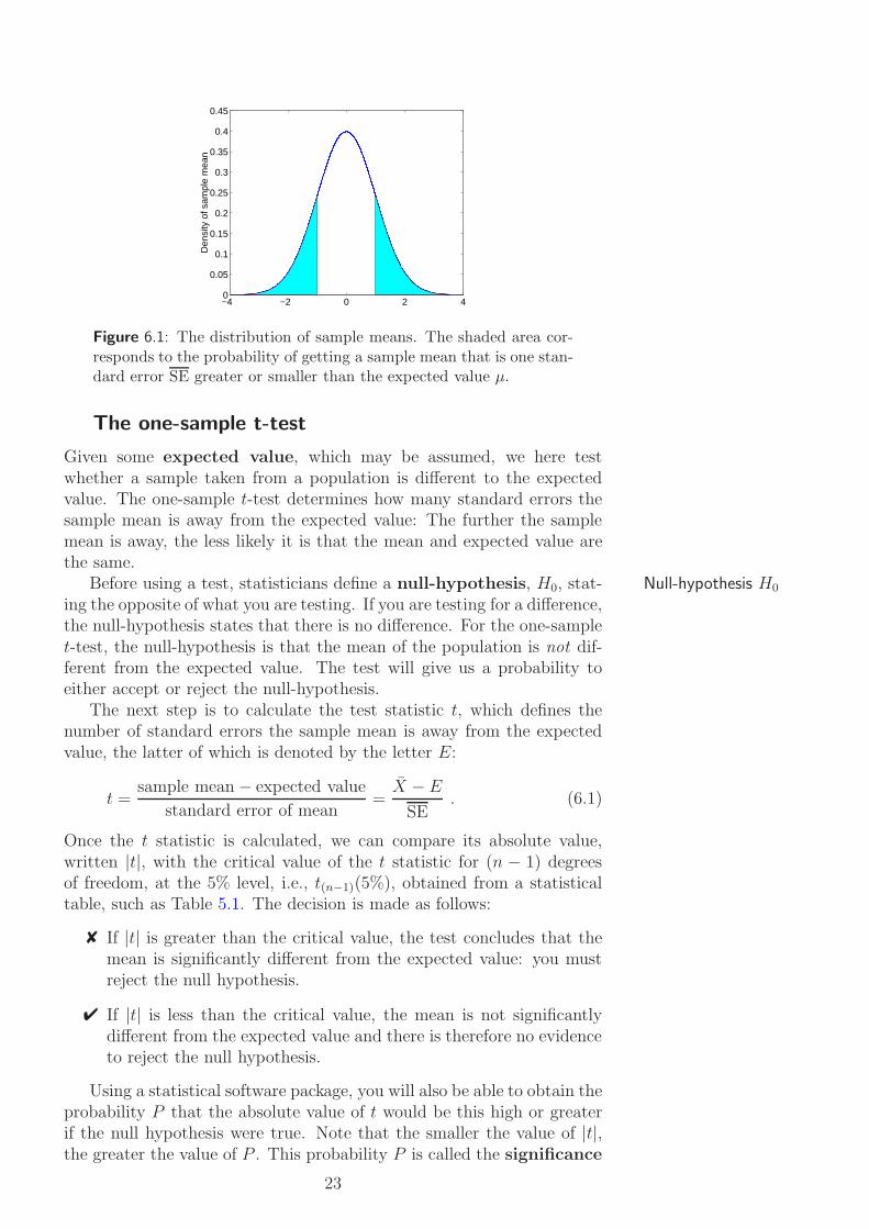
With the material of the previous sections we have now available some ofthe tools that are necessary for the most frequent application of statisticsin biology: testing a hypothesis related to a sample of data. The purposeof statistical hypothesis testing is to establish significance tests helping Hypothesis testingus in decision making and quantifying the uncertainty in this process. Forexample, taking two separate samples, we wish to compare the averagevalues and test whether they are different. From the previous section, weknow that sample means itself vary and a numerical difference betweentwo sample means does not necessarily mean that this corresponds to adifference in the population means. The difference between two samplemeans may happen by chance. Figure 6.1, illustrates the probability ofgetting a sample mean that is one standard error SE greater or smallerthan the expected value µ.
In the following we consider three tests for different scenarios: testingthe difference between a sample and an expected value, testing the dif-ference between two samples from the same population, and testing thedifference between two samples from two populations. Since the test weconsider here involve inferences about population parameters, they arealso referred to as parametric tests. The t-tests are valid for relatively Parametric testssmall samples (n < 30).
22
−4 −2 0 2 40
0.05
0.1
0.15
0.2
0.25
0.3
0.35
0.4
0.45
Den
sity
of s
ampl
e m
ean
Figure 6.1: The distribution of sample means. The shaded area cor-responds to the probability of getting a sample mean that is one stan-dard error SE greater or smaller than the expected value µ.
The one-sample t-test
Given some expected value, which may be assumed, we here testwhether a sample taken from a population is different to the expectedvalue. The one-sample t-test determines how many standard errors thesample mean is away from the expected value: The further the samplemean is away, the less likely it is that the mean and expected value arethe same.
Before using a test, statisticians define a null-hypothesis, H0, stat- Null-hypothesis H0
ing the opposite of what you are testing. If you are testing for a difference,the null-hypothesis states that there is no difference. For the one-samplet-test, the null-hypothesis is that the mean of the population is not dif-ferent from the expected value. The test will give us a probability toeither accept or reject the null-hypothesis.
The next step is to calculate the test statistic t, which defines thenumber of standard errors the sample mean is away from the expectedvalue, the latter of which is denoted by the letter E:
t =sample mean − expected value
standard error of mean=
X − E
SE. (6.1)
Once the t statistic is calculated, we can compare its absolute value,written |t|, with the critical value of the t statistic for (n − 1) degreesof freedom, at the 5% level, i.e., t(n−1)(5%), obtained from a statisticaltable, such as Table 5.1. The decision is made as follows:
✘ If |t| is greater than the critical value, the test concludes that themean is significantly different from the expected value: you mustreject the null hypothesis.
✔ If |t| is less than the critical value, the mean is not significantlydifferent from the expected value and there is therefore no evidenceto reject the null hypothesis.
Using a statistical software package, you will also be able to obtain theprobability P that the absolute value of t would be this high or greaterif the null hypothesis were true. Note that the smaller the value of |t|,the greater the value of P . This probability P is called the significance
23

probability. In many textbooks this is also referred to as the P -value or Significance probability“achieved significance level”. In general, the P -value is the probability P -valueof observing the given sample result under the assumption that the null-hypothesis is true. Using some statistical programme, you can make yourdecisions depending on the significance probability instead of using thetable:
✘ If P < 0.5, the null hypothesis should be rejected.
✔ If P ≥ 0.5, there is no evidence to reject the null hypothesis.
Finally, you can calculate the 95% confidence limits for the differenceby using the following equation:
95% CI(difference) = X − E ± (t(n−1)(5%) × SE)
. (6.2)
Example: Ten independent observations are taken from a normaldistribution with mean µ. The sample variance is s2 = 40 and thesample mean is X = 16. We wish to test whether the sample meanis significantly different from the expected value. The hypotheses aretherefore
• Null hypothesis: µ = 20
• Alternative hypothesis: µ �= 20.
The standard error of the sample mean is
SE =s√n
=6.325
3.162= 2 .
The t-statistic is
t =16 − 20
2= −2 .
In other words, the sample mean is −2 standard errors away from theexpected value. From Table 5.2, for a 1% significance level we look at thecolumn for α = 0.005 and row ν = 9, to obtain tα,ν = t0.005,9(1%) = 3.25.Since |t| is much less than the critical value, we have no evidence to rejectthe null hypothesis and conclude that the sample mean is not significantlydifferent from the expected value.
The 99% confidence interval for the difference is calculated as
99% CI(difference) = 16− 20± (3.25 · 2) = −4± 6.5 = [−10.5, 2.5] .
In other words, 99% of all observed differences would be expected to lie inthis interval. Note that the sample mean obtained here does not fall intothis range and that this conclusion is quite independent of the decisionto accept or reject the null hypothesis.
Example: The mean time taken for a plant to die when treated witha solution is known to be 12 days. When the solution dose was twice asmuch in a sample of ten plants, the survival times were 10, 10.7, 12.4,12.2, 9.8, 9.9, 10.4, 10.8, 10.1, 11.2.
24

If the survival times are following a Normal distribution, test whetherthe results suggest that the increased solution dosage does lead to adecreased survival time. If we denote the mean survival time for doublethe dose with µ, then the null hypothesis H0 is µ = 12 and the alternativehypothesis H1 is µ < 12 (Note the difference to the previous example!):
H0 : µ = 12
H1 : µ < 12 .
Choosing a 1% significance level, we are going to look for critical regionin one tail of the t-distribution (because of H1). The 1% significance levelmeans that we are looking for an area in the left tail of the t-distributionwhich has probability 0.01 (a one-sided hypothesis test). The samplemean
X =1
10·
10∑i=1
xi = 10.75
The sample variance
s2 =1
9
10∑i=1
x2i −10X2 =
1163.39 − 1155.625
9= 0.863 and s = 0.93 .
The value of the t-statistic will be
t =10.75 − 12
0.93/√
10=
−1.25
0.29= −4.31 .
From Table 5.2, for ν = 9, (the table provides values for positive ts), thecritical region in the left tail of the t-distribution is for values of t smallerthan −2.821. Since the value t = −4.31 is much further to the left in thecritical region, H0 is rejected. In other words, doubling the dose reducesthe survival time of the plants.
Note: The choice of the null hypothesis should be made before thedata are being analysed as otherwise one might introduce a bias into theanalysis. We speak of a one-sided hypothesis if we test for a statisticbeing greater or smaller than a value (e.g. µ > 0.3) and a hypothesis iscalled two-sided if we test whether the statistic is different to a value(e.g. µ �= 0.3).
Remark: You should read the following definitions carefully and try toremember them. The P-value is the probability of the observed data (ordata showing a considerable departure from the null hypothesis) whenthe null hypothesis is true. The P -value is not the probability of thenull hypothesis nor is it the probability that the data have arisen bychance. The significance level is the level of probability at which itis agreed that the null hypothesis will be rejected. Conventionally thisvalue is set to 0.05. A significance test is then a statistical procedurethat when applied to a set of data results in a P -value relative to somehypothesis.
25

PRACTICE. Using following data set [7],
4.5 5.2 4.9 4.3 4.6 4.8 4.6 4.94.5 5.0 4.8 4.6 4.6 4.7 4.5 4.7
1. estimate the population mean and variance.
2. decide whether the sample mean is significantly different from apopulation with a mean value of 4.5.
3. use a statistical software package, such as MS Excel to calculate theP -value (significance probability).
4. use Table 5.1 to obtain the critical value of t at the 5% significancelevel.
5. calculate the 95% confidence limits for the difference.
The paired t-test
With the paired t-test we compare the means from two samples obtainedfrom what we consider to be a single population. For example, you maytake two samples at different times from the same culture (colony, or Petridish). Other typical experiments for which this test is used include “be-fore/after” or “treated/untreated” descriptions of the experiment. LetXA and XB denote the two samples, d is the difference, XA −XB, of thetwo samples, and d is the average, 1/n
∑d, of the differences. As with
the one-sample t-test, the steps to follow are:
Step 1: The null-hypothesis is that the mean difference, d is not differ-ent from zero.
Step 2: The test statistic t is the number of standard errors the differ-ence is away from zero:
t =mean difference
standard error of difference=
d
SEd
where
SEd =sd√n
.
Step 3: Calculate the significance probability P that the absolute valueof the test statistic would be equal or greater than t if the nullhypothesis were true. Using a statistical table, compare the value|t| calculated above with the critical value of the t statistic for(n − 1) degrees of freedom and at the 5% level, i.e., t(n−1)(5%).The bigger the value of |t|, the smaller the value of P .
Step 4: Hypothesis testing:
✘ If |t| is greater than the critical value, the null hypothesis isrejected: The mean difference is significantly different fromzero.
26

✔ If |t| is less than the critical value, then there is no evidenceto reject the null hypothesis.
Using a statistical software package,
✘ If P < α = 0.05, reject the null hypothesis.
✔ If P ≥ α = 0.05, there is no evidence to reject the null hy-pothesis, the mean difference is not significantly different fromzero.
Step 5: Calculate the 95% confidence limits for the mean difference as
95% CI(difference) = d ± (t(n−1)(5%) × SEd
).
Since the decision whether to accept or reject a hypothesis is madeon the basis of data that are randomly selected, an incorrect decision ispossible. If we reject the null hypothesis H0 when it is true, this is calleda Type I error. Similarly, if we accept H0 when it is false, we commit Type I errora Type II error. By choosing α (usually 1% or 5%) we fix the Type I Type II errorerror to some acceptable low level. If the P -value is less than the chosenType I error, the null hypothesis is rejected.
The two-sample t-test
The purpose of this test is to decide whether the means of two samplesobtained from two populations are different from each other. We assumethat both samples are independent of each other. For example, thistest does not apply to samples taken from the same culture.
Both sample means will have a distribution associated with it, andas illustrated in Figure 6.2, the test effectively tests the overlap betweenthe distributions of the two sample means. Here we consider only thecase, when it is reasonable to assume that the two populations havethe same variance. (Most software packages will have available testsfor populations with different variances.)
Step 1: The null-hypothesis is that the mean of the differences is notdifferent from zero. In other words, the two groups A and B fromwhich the samples were obtained have the same mean.
Step 2: The test statistic t is given by the following formula:
t =mean difference
standard error of difference=
XA − XB
SEd
The standard error of the difference SEd is more difficult to cal-culate because this would involve comparing each member of thefirst population with each member of the second. Assuming thatthe variance of both populations is the same, we can estimate SEd
using the following equation:
SEd =
√(SEA
)2+(SEB
)2,
where SEA and SEB are the standard errors of the two populations.
27

0
0.05
0.1
0.15
0.2
0.25
0.3
0.35
0.4
dens
ity o
f sam
ple
mea
ns
sample mean of A sample mean of B
Figure 6.2: In the two-sample t-test, we wish to decide whether themeans of two samples, obtained from two populations are different. Inother words, we wish to quantify the overlap between the distributionsof the sample means.
Step 3: Calculate the significance probability P that the absolute valueof the test statistic would be equal to or greater than t if the nullhypothesis were true. There are nA + nB − 2 degrees of freedom,where nA and nB are the sample sizes of groups A and B.
Step 4: Using a statistical software package,
✘ If P < 0.05, reject the null hypothesis, the sample means aresignificantly different from each other.
✔ If P ≥ 0.05, there is no evidence to reject the null hypothesis,the two sample means are not significantly different from eachother.
Step 5: The 95% confidence interval for the mean difference is given by
95% CI(difference) = XA − XB ± (t(nA+nB−2)(5%) × SEd
).
Example: We obtain two independent samples XA, XB and we wishto calculate the 95% confidence interval for the difference of the twogroup means:
XA = {64, 66, 89, 77}, XB = {56, 71, 53} .
We calculate XA = 296/4 = 74 and XB = 180/3 = 60, sA = 11.5181 andsB = 9.643; SEA = 5.7591, SEB = 5.5678; SEd = 8.01. Thus,
95% CI(difference) = 74 − 60 ± (2.571 · 8.01) = 14 ± 21 .
Example: In an experiment we are comparing an organism for whichthe cells were generated by two independent methods (A and B). At acertain stage of the development the length is measured. The data aresummarised in Table 6.1. If the lengths are following a Normal distribu-tion, we wish to test whether they are significantly different for the twogroups. The hypotheses are:
H0 : µA = µB
H1 : µA �= µB .
28

Table 6.1: Experimental data set.Origin length (mm) ± s (mm)A 87.04 ± 7.15B 77.77 ± 4.70
We have A = 87.04, B = 77.77, sA = 7.15, sB = 4.70 and thus
SE2
A =s2
A
nA= 2.56, SE
2
B =s2
B
nB= 1.10, SEd =
√SE
2
A + SE2
B = 1.91
and therefore
t =A − B
SEd
= 4.84 .
Choosing a 1% significance level, we find that for ν = 38 most tables willnot list the desired values. We can however interpolate (from tables likeTable 5.2 [1]) such that if values are given for say ν = 30 and ν = 40, thisgives us a range for the t-statistic to lie between approximately −2.72and 2.72 for H0 to be accepted. Since 4.84 is considerably larger than2.72, the null hypothesis is rejected.
The calculation of the t-statistic for the two-sample t-test can bedone in different ways and textbooks will sometimes provide the followingdescription of Step 2: If the null hypothesis is correct, the following t-statistic has a Student’s t-distribution with ν = nA + nB − 2 degrees offreedom:
t =XA − XB
sp ·√
1nA
+ 1nB
where sp =
√(nA − 1)s2
A + (nB − 1)s2B
nA + nB − 2
Apart from the different calculation there is no change, i.e., using a statis-tical table for the t-distribution, we would check whether the calculatedt-statistic falls into the critical region.
Equation using sp is based on the idea, that since we assume thatboth samples have the same variance, we can ‘pool’ them:
s2p =
∑(nA − 1)2 +
∑(nB − 1)2
(nB − 1) + (nB − 1).
Since
s2A =
∑(XA − XA)
2
nA − 1and s2
B =
∑(XB − XB)
2
nB − 1,
we have
s2p =
(nA − 1)s2A + (nB − 1)s2
B
nA + nB − 2or sp =
√(nA − 1)s2
A + (nB − 1)s2B
nA + nB − 2.
As an exercise you should compare the two different strategies and com-pare the difference.
29

Note: If you want to compare the means of more than two groups, youcannot use the t-test. For this case, a more sophisticated test, calledANOVA test (analysis of variance) is available. We have also not con-sidered experiments associated with distributions others than the Normaldistribution. Statistical t-tests are valid for small sample sizes (say n lessthan 30). For larger samples z-tests should be used.
Remark: One usually doesn’t learn about the origins of a mathematicalconcept although in statistics it is often rather interesting to know howthe various, often alternative, techniques have developed. The followingstory about the t distribution and test is frequently told. William SealyGosset (1876 - 1937) studied chemistry at Oxford University and laterworked for the Guinness brewery. Investigating the relationship betweenthe final product and the raw materials, he developed the statistics wehave discussed here. The company did not allow publications of thisnature and he choose a pseudo name ‘student’. Many textbooks willstill refer to the distribution as the ‘students t distribution. Why hechoose to call it a ‘t’-test when he was working with beer is unknown...
7 Categorical Data: The Chi-Square Test
The chi-squared (χ2) test is used to determine whether there are differ-ences between real and expected frequencies in one set of categories, orassociations between two sets of categories. Also, in previous sections wehave assumed that a particular type of distribution is appropriate for thethe data. We then estimated parameters of this distribution and testedhypotheses about parameters.
Categorical data are data that are not numbers but measurementsassigned to categories. Examples of character states are the colour Character statesof objects, conditions like dead/alive or healthy/diseased. Data withequal character states form categories. Categorical data is quantified bythe frequency with which each category was observed. Similar to thet-tests, we can as the following questions:
� Are observed frequencies in a single group different from expectedvalues?
� Are observed frequencies in two or more groups different from eachother?
To answer these questions we have two tests available: the χ2 test fordifferences and the χ2 test for association.
Chi square test for differences
The purpose of this test is to decide whether observed frequencies aredifferent from expected values. The χ2 statistic calculated here is a mea-sure of this difference. The null hypothesis is that the frequencies of thedifferent categories in the population are equal to the expected frequen-cies. Critical values or percentage points of the χ2 distribution can befound in tables of the same nature as Tables 5.1, 5.2.
30

The χ2 statistic is calculated by the expression
χ2 =∑ (O − E)2
E,
where O is the observed frequency and E is the expected frequency foreach character state (category). The larger the difference between thefrequencies, the larger the value of χ2 and the less likely it is that observedand expected frequencies are different just by chance. Different sampleswill give different observed frequencies and hence different values for χ2.Thus χ2 has a probability distribution which is illustrated in Figure 7.1.(Actually, there is a small difference between the expression (7.2) andthe distribution in Figure 7.1, but since I referred to Figure 7.1 as anillustration this may not be a problem.).
0 5 10 15 200
0.1
0.2
0.3
0.4
0.5
χ2 den
sity
1 d.f.
2 d.f.
4 d.f.
8 d.f. 16 d.f.
Figure 7.1: Chi square, χ2 distribution with different degrees of free-dom. In practise one would not use such graph but tables to obtainvalues required for calculations.
The probability P of obtaining χ2 values equal or greater than theobserved values if the null hypothesis were true can be obtained fromtables which list the critical value that χ2 must exceed at (N −1) degreesof freedom, where N is the number of groups, for the probability to beless than 5%.
Note: The distribution of χ2 is depends on the number of degreesof freedom - the bigger the sample you take, the more likely you will beto detect any differences. Note that therefore the two tests we introducehere are only valid if all expected values are larger than 5.
Chi square test for association
With this test we wish to decide whether the character frequencies of twoore more groups are different from each other. In other words, we testwhether character states are associated in some way. The test investigateswhether the distribution is different from what it would be if the characterstates were distributed randomly among the population.
The null hypothesis is that there is no difference between the frequen-cies of the groups, hence no association between the character states.Before we can calculate the χ2 statistic we must calculate the expected
31

values for each character state if there had been no association. To do Contingency tablethis we arrange the data in a contingency table:
Character a Character b TotalGroup A frequency frequencyGroup B frequency frequencyTotal
The expected number E (frequency) if there had been no associationbetween the character states in the two groups is given by
E =column total × row total
grand total(7.1)
The grand total is the sum of the two row totals. The significance prob-ability is obtained from a statistical table as the critical value that χ2
must exceed at (R − 1) × (C − 1) degrees of freedom, where R is thenumber of rows in the table above and C is the number of columns, forthe probability to be less than 5%. If χ2 is greater than the critical value,the null hypothesis is rejected - there is a significant associations betweenthe characters.
PRACTICE. Through experiments on two groups we found that in groupA, out of 30 objects, 18 had character state a and 12 had character stateb, while of the 60 objects in group B, 12 had character state a and for48 objects we observed character state b. Test whether character state ais significantly different in the groups. Using a software package such asMinitab, MS Excel, Matlab or Mathematica,
1. formulate the null hypothesis.
2. calculate the test statistic.
3. determine the P -value.
4. decide whether to reject the null hypothesis.
Chi-square test for goodness of fit
The χ2 test can also be used to determine how well theoretical distribu-tions (such as the Normal distribution) fit empirical distributions (i.e.,those obtained from sample data). As in previous sections, a measure forthe goodness of fit of the model can be established with the followingstatistic:
χ2 =
m∑i=1
(Oi − Ei)2
Ei, (7.2)
where m denotes the number of different outcomes. Significantly largevalues of χ2 suggest a lack of fit. We are now going to see how the chi-square statistic can be used to test whether a frequency histogram fitsthe normal distribution.
32

Fitting a normal curve to the data of Table 2.1, we first calculatestandard units for the class boundaries, z = (x− X)/s. The areas underthe normal curve can be obtained from tables (e.g. Table 4.1). From thiswe find the areas under the normal curve between successive values of z asshown in column 5 of Table 7.1. These are obtained by substracting thesuccessive areas in column 4 when the corresponding z’s have the samesign, and adding them when the z’s have opposite sign. Multiplying theentries in column 5 (rel. freq.) by the total frequency (n = 100) givesus the expected frequencies, as shown in column 6. To determine thegoodness of fit, we calculate
χ2 =(5 − 4.13)2
4.13+
(18 − 20.68)2
20.68+
(42 − 38.92)2
38.92
+(27 − 27.71)2
27.71+
(8 − 7.43)2
7.43= 0.059
Since the number of parameters used in estimating the expected frequen-cies is 2, we have ν = 5− 1− 2 = 2 degrees of freedom. From a table wefind χ2
.95 = 5.99. Thus we can conclude that the fit of the data is good.
Table 7.1: Fitting a normal curve to the data in Table 4.1 and test-ing the fit of the frequency histogram in Figure 2.2 to the normaldistribution [5].
classlimits
classboundaries
z for classlimits
area undernormal curvefrom 0 to z
area foreach class
expectedfrequency
observedfrequency
60-62 59.5 -2.72 0.4967 0.0413 4.13, or 4 563-65 62.5 -1.70 0.4554 0.2068 20.68, or 21 1866-68 65.5 -0.67 0.2486 0.3892 38.92, or 39 4269-71 68.5 0.36 0.1406 0.2771 27.71, or 28 2772-74 71.5 1.39 0.4177 0.0743 7.43, or 7 8
74.5 2.41 0.4920
Note: In this section, we introduced only the most basic concepts forcategorical data. Books in the reference list (Section 13, page 39) willprovide more details on the rationale behind the tests and will help you inselecting an appropriate test for a problem at hand. Another importantissue, which we haven’t dealt with, is the design of experiments.
8 Finding Associations: Correlation
... have a look at the references given in Section 13.
9 Modelling Relationships: Linear Regression
... have a look at the references given in Section 13.
33

10 More Exercises
Exercises for Section 2
The following sample consists of 12 temperature measurements takenevery two hours: −2,−3,−3,−2, 0, 4, 5, 6, 6, 6, 3, 1. Calculate
1. The temperature average of the day, i.e., the sample mean X. Dothree calculations:
(a) Using equation (3.1).
(b) Using equation (3.2).
(c) Using the statistical function of your calculator.
2. The sample variance σ2n, the sample standard deviation σn, and the
unbiased estimate of the population variance s2:
(a) Using equations (3.3) and (3.4).
(b) Using equation (3.5).
(c) Using the statistical functions of your calculator.
50, 35, 19, 27, 44, 70, 60, 28, 61, 41, 50, 5661, 52, 62, 66, 70, 52, 81, 43, 63, 52, 71, 5160, 35, 49, 57, 44, 30, 60, 28, 61, 44, 55, 3651, 62, 42, 66, 70, 42, 61, 43, 63, 52, 71, 5150, 75, 44, 65, 44, 70, 60, 67, 65, 44, 55, 57
Table 10.1: Exam results for 60 students.
Table 10 lists the exam results for 60 students. For the given data set,
1. Calculate the range of the scores.
2. Construct the tally chart for the following score intervals
score tallies0 − 9 ||||
10 − 1920 − 2930 − 3940 − 4950 − 5960 − 6970 − 7980 − 8990 − 100
3. Determine the relative frequency distribution for the intervals spec-ified above.
4. Visualise the relative frequency distribution with a relative fre-quency histogram.
5. Calculate and draw the cumulative frequency distribution.
34

Exercises for Section 3
For the data in Table 10,
1. Calculate the mean, the median, the mode and the standard devi-ation using your calculator or a software package.
2. Mark the calculated statistics in the relative frequency histogramcalculated previously.
3. The nth percentile is the score that leaves n% of the data to the left.Calculate the 10th, 30th, 60th, and 90th percentiles. Hint: Sort thedata from the smallest to the largest value. Mark the percentilesin the relative frequency histogram.
Exercises for Section 4
1. For the distribution of the scores of Table 10 answer the followingquestions,
(a) is the distribution unimodal?
(b) is the distribution symmetric about the mean?
(c) calculate the percentage of observations falling between X +0.674s
(d) calculate the percentage of observations falling between X +1.96s
(e) calculate the percentage of observations falling between X +2.576s
2. Do you think that the scores of Table 10 are “normally distributed”(follow a normal or Gaussian distribution)?
3. Are the scores in Table 10.2 “more” normally distributed than thosein Table 10?
53, 63, 52, 63, 61, 69, 60, 53, 56, 59, 62, 6155, 58, 60, 60, 51, 59, 59, 65, 61, 59, 67, 7160, 59, 69, 55, 44, 60, 59, 57, 58, 69, 56, 7460, 57, 60, 60, 54, 46, 54, 59, 66, 63, 54, 6458, 61, 68, 61, 52, 58, 62, 63, 66, 73, 57, 63
Table 10.2: Data set.
Exercises for Section 5
You read in a scientific report that the average age of death for womenin your country is 73.2 years. To find out whether the average age ofdeath for men is the same as that of women, a small sample of 25 deathcertificates shows an average age of 58.4 years and a sample standarddeviation of 15 years.
35

1. Using a significance level of 0.01, choose an appropriate hypoth-esis test and determine whether the null hypothesis (there is nodifference between mean and woman) should be accepted.
2. Use the 99% confidence interval for the men’s average age of deathto reach the same conclusion.
Exercises for Section 6
1. A researcher believes that the average weight in a group of peopleis 120 pounds. To test this belief, you determine the weight of 7people with the following results (in pounds)): 121, 125, 118, 130,117, 123, and 120.
(a) Estimate the population mean and variance.
(b) Decide whether the sample mean is significantly different froma population with a mean value of 120.
(c) Obtain the critical value of t at the 5% significance level.
(d) Calculate the 95% confidence limits for the difference.
2. Imagine you want to test whether or not six minutes is enoughtime for the heart to recover the pulse rate after two minutes ofexercise. For a period of one week the pulse rate is measured fromone person, every day, before exercise and six minutes after theexercise, obtaining the data summarised in Table 10.3. Do thesedata indicate that the heart rate after the exercise is higher thanbefore the exercise? Use a 1% level of significance.
Test 1 2 3 4 5 6Before 69 72 75 73 70 74After 85 79 83 84 87 78
Table 10.3: Data set.
3. We want to compare the efficiency of the two pieces of equipment,referred to as A and B. In Table 10.4 the first row shows thenumerical values obtained for the efficiency measure for meter Aand the second row show the results for meter B.
(a) Calculate the mean and the standard deviation for each group.
(b) Calculate the 95% confidence interval for the difference of thetwo group means
(c) What can you say about the efficiency of the two meters?
A 18 15 18 16 17 15 14 14 14 15B 24 27 27 25 31 35 24 19 28 23
Table 10.4: Data set.
36

11 Solutions to Exercises in Section 10
Solutions to Section 10, related to Section 5
1. SE = s√n
= 15√25
= 3
t = X−ESE
= 68.4−73.23
= −1.6, | t |= 1.6t(24)(1%) from the table is 2.797, so we do not reject the null hy-pothesis.
2. 99%CI = X ± (t(24)(1%) × SE)99%CI = 68.4 ± (2.797 × 3)99%CI = 68.4 ± 8.3910The women’s average age of death is included in the range.
Solutions to Section 10, related to Section 6
1. Sample mean X = 8547
= 122Estimated population variance s2 = 20Estimated population standard deviation s = 4.472SE = s√
n= 4.472√
7= 1.690
t = X−ESE
= 122−1201.690
= 1.832, | t |= 1.832t(6)(5%) from the table is 2.447, so we do not reject the null hy-pothesis.99%CI = X − E ± (t(6)(5%) × SE)99%CI = 122 − 120 ± (2.447 × 1.690)99%CI = 2 ± 4.1352
2. d = XA − XB
d = 1n
∑d = 10.5
SEd = sd√n
= 2.110
t = dSEd
= 10.52.110
= 4.977, | t |= 4.977
t(5)(1%) from the table is 4.032, so we reject the null hypothesis.
3. SEA = SA√n
= 1.5776√10
= 0.4989,
SEB = SB√n
= 4.4485√10
= 1.4067,
SEd =
√SE
2
A + SE2B = 1.4926
95%CI = XA − XB ± (t(18)(5%) × SEd)95%CI = 15.6 − 26.3 ± (2.101 × 1.4926)95%CI = −10.70 ± 3.136t = XA−XB
SEd= 15.6−26.3
1.4926= −7.1687, | t |= 7.1687
t(18)(5%) from the table is 2.101 so the means are different.
37

12 Symbols and Notation
The following symbols are used in the notes. They are listed in the orderof their appearance.
A, B samples or groups,F (x) cumulative distribution function.X sample.
xi ∈ X element, observation or measurement in sample.{ } list, set.n sample size (number of elements in sample).X sample mean.µ population mean.σ2
n sample variance.s2 = σ2
n−1 unbiased estimator of population variance.σ2 population variance.
σ =√
σ2 population standard deviation.∑ni=1 sum of elements with index i = 1, 2, . . . , n.fi frequency of observation (of xi or in class i).m number of distinct value of x in a sample.
p(x) probability density function.P (·) probability.[a, b] interval ranging from a to b.
z standard unit.Φ(z) cum. distr. fcn. of standardized normal variable z.SE standard error.
SE estimated standard error.CI confidence interval.d.f. degrees of freedom. See also ν.
t(n−1)(·) critical value of t distribution.t t statistic.α 100% percentage point (of t distribution).ν degree of freedom.E expected value, expected frequency.| · | absolute value.d difference.d average of differences.P P -value.
H0, H1 null hypothesis, alternative hypothesis.SEd standard error of mean difference.χ2 chi-square distribution and test.O observed frequency.N number of groups.
R, C number of rows and columns in contingency table.
38

13 Further Reading
There are many statistics books available and I strongly recommend tobuy at least one. The small book by Rowntree [3] is the most basicand yet very good introduction for those who are worried about themathematics. It shows that ideas come first, and equations should onlyfollow as a means towards an end. Since there are so many differenttechniques and concepts in statistics, it is very important to ask the‘right’ question in order to identify a suitable technique, test or tool.Freedman’s [4] is a very good book in this respect too but much morecomprehensive. [2] has many exercises and is at an introductory level.The Schaum Outline [5] is one of a series of well known introductory textsto mathematics. Wonnacott and Wonnacott [6] is a hardcover text andis likely to last a little longer. Although the area from which examplesare taken shouldn’t matter too much for an introductory book, here thefocus is on examples from business and economics. It has exercises and issuitable as a basic reference. Previous books contained general examplesfrom science, engineering, economics etc, while [7] is a well written basicintroduction for biologists - good value for money too. The recent bookby Quinn and Keough [9] is a comprehensive treatment that is written forbiologists. It is a textbook that is also a good reference. In addition to thebasic statistics, it covers multivariate data analysis (clustering, principalcomponent analysis,...) and regression techniques. Finally, Sokal andRohlf [8] wrote one of the most comprehensive statistics book aimed atbiologists. It is a very good but also advanced reference book.
39

Bibliography
[1] Murdoch, J. and Barnes, J.A. (1974): Statistical Tables for Science,Engineering, Management and Business Studies. 2nd ed. Macmillan,London.
[2] Upton, G. and Cook, I. (2001): Introducing Statistics. Oxford Uni-versity Press. 470 pages. ISBN 9 780199 148011. £22
[3] Rowntree, D. (1981): Statistics without Tears. Penguin. 199 pages.ISBN 0 14 013632 0. £7
[4] Freedman, D. and Pisani, R. and Purves, R. (1998): Statistics. W.W.Norton & Company. 700 pages. ISBN 0 393 97121 X. £19
[5] Spiegel, M.R. and Stephens, L.J. (1998): Statistics. Schaum’s Out-lines. 538 pages. ISBN 0 07 060281 6. £12
[6] Wonnacott, T.H. and Wonnacott, R.J. (1990): Introductory Statis-tics. John Wiley & Sons. 711 pages. ISBN 0 471 61518 8. £16
[7] Ennos, R. (2000): Statistical and Data Handling Skills in Biology.Prentice Hall. 132 pages. ISBN 0 582 31278 7. £10
[8] Sokal, R.R. and Rohlf, F.J. (1995): Biometry. W.H. Freeman andCompany. 887 pages. ISBN 0 7167 2411 1. £38
[9] Quinn, G.P. and Keough, M.J. (2002): Experimental design andData Analysis for Biologists. Cambridge University Press. 537 pages.ISBN 0 521 00976 6. £30
40