Data Flow Analysis In Software Reliability* LLOYD D. FOSDICK and LEON J. OSTERWEIL

D a t a F low Analys is In S o f t w a r e R e l i a b i l i t y *

LLOYD D. FOSDICK

and

LEON J. OSTERWEIL

Department of Computer ~cience, University of Colorado, Boulder, Colorado 80809

The ways that the methods of data flow analysis can be applied to improve software reliability are described. There is also a review of the basic terminology from graph theory and from data flow analysis in global program optimization. The notation of regular expressions is used to describe actions on data for sets of paths. These expressions provide the basis of a classification scheme for data flow which represents patterns of data flow along paths within subprograms and along paths which cross subprogram boundaries. Fast algorithms, originally introduced for global optimization, are described and it is shown how they can be used to implement the classification scheme. It is then shown how these same algorithms can also be used to detect the presence of data flow anomalies which are symptomatic of programming errors. Finally, some characteristics of and experience with DAVE, a data flow analysis system embodying some of these ideas, are described.

Keywords and Phrases: automatic documentation, automatic error detection, data flow analysis, software reliability CR Categories: 4.40, 5.24

INTRODUCTION

For some t ime we have believed tha t a careful analysis of the use of data in a program, such as tha t done in global optimization, could be a powerful means for detecting errors in software and otherwise improving its quality. Our recent experience [27, 28] with a system constructed for this purpose confirms this belief. As so often happens on such projects, our knowledge and understanding of this approach were deepened considerably by the experience gained in constructing this system, although the pressures of meeting various deadlines made it impossible to incorporate all of our developing ideas into the system. More-

* This work supported by NSF Grant DCR 754)9972.

over, during its construction advances were made in global optimization algorithms tha t are useful to us, which for the same reasons could not be incorporated in the system. Our purpose in writing this paper is to draw these various ideas together and present them for the instruction and stimu- lation of others who are interested in the problem of software reliability.

The phrase "da ta flow analysis" became firmly established in the li terature of global program optimization several years ago through the work of Cocke and Allen [2, 3, 4, 5, 6]. Considerable at tent ion has also been given to data flow b y Dennis and his co-workers [9, 29] in a different context, advanced computer architecture. Our own interpretation of data flow analysis is simi-

Copyright © 1976, Association for Computing Machinery, Inc. General permission to republish, but not for profit, all or part of this material is granted provided that ACM's copyright notice is given and that reference is made to the publication, to its date of issue, and to the fact that reprinting privileges were granted by permission of the Association for Computing Machinery.

Computing Surveys, Vol. 8, No. 3, September 1976

306 • Data Flow Analysis In Software

CONTENTS

INTRODUCTION BASIC DEFINITIONS--GRAPHS BASIC DEFINITIONS--PATH EXPRESSIONS TO

REPRESENT DATA FLOW ALGORITHMS TO SOLVE T H E LIVE VARIABLE

PROBLEM AND T H E AVAILABILITY PROBLEM SEGMENTATION OF DATA FLOW DETECT IN G ANOMOLOUS PATH EXPRESSIONS CONCLUSION ACKNOWLEDGMENTS REFERENCES

T

lar to that found in the literature of global program optimization, but our emphasis and objectives are different. Specifically, execution of a computer program normally implies input of data, operations on it, and output of the results of these operations in a sequence determined by the program and the data. We view this sequence of events as a flow of data from input to output in which input values contribute to intermediate results, these in turn contribute to other intermediate results, and so forth until the final results, which presumably are output, are obtained. It is the ordered use of data implicit in this process that is the central object of study in data flow analysis.

Data flow analysis does not imply execution of the program being analyzed. In- stead, the program is scanned in a systematic way and information about the use of variables is collected so that certain in- ferences can be made about the effect of these uses at other points of the program. An example from the context of global optimization will illustrate the point. This example, known as the live variable problem, determines whether the value of some variable is to be used in a computation

Reliability

after some designated computation step. If it is not to be used, space for that variable may be reallocated or an unnecessary assignment of a value can be deleted. To make this determination it is necessary to look in effect at all possible execution sequences starting at the designated execution step to see if the variable under consideration is ever used again in a computation. This is a difficult problem in any practical situation because of the complexity of execution sequences, the aliasing of variables, the use of external procedures, and other factors. Thus a brute force attack on this problem is doomed to failure. Clever algorithms have been developed for dealing with this and related problems. They do not require explicit consideration of all execution sequences in the program in order to draw correct conclusions about the use of variables. Indeed, the effort expended in scanning through the program to gather information is remarkably small. We discuss some of these algorithms in detail, because they can be adapted to deal with our own set of problems in software reliability, and turn to these problems now.

Data flow in a program is expected to be consistent in various ways. If the value of a variable is needed at some computation step, say the variable a in the step

'y ~--- a-t- 1,

then it is normally assumed that at an earlier computation step a value was assigned to a. If a value is assigned to a variable in a computation step, for example to ~, then it is normally assumed that that value will be used in a later computation step. When the pattern of use of variables is abnormal, so that our expectations of how variables are to be used in a computation are violated, we say there is an anomaly in the data flow. Examples of data flow anomalies are illustrated in the following FORTRAN constructions. The first is

X = A X = B


I t is clear that the first assignment to X is useless. Why is the statement there at all? Perhaps the author of the program meant to write

X = A Y = B

Another data flow anomaly is represented by the FORTRAN construction

SUBROUTINE SUB(X, Y, Z) Z = Y + W

Here W is undefined at the point that a value for it is required in the computation. Did the author mean X instead of W, or W instead of X, or was W to be in COM- MON? We do not know the answers to these questions, but we do know that there is an anomaly in the data flow.

As these examples suggest, common programming errors cause data flow anomalies. Such errors include misspelling, con- fusion of names, incorrect parameter usage in external procedure invocations, omission of statements, and similar errors. The presence of a data flow anomaly does not imply that execution of the program will definitely produce incorrect results; it implies only that execution may produce incorrect results. I t may produce incorrect results depending on the input data, the operating system, or other environmental factors. I t may always produce incorrect results regardless of these factors, or it may never produce incorrect results. The point is that the presence of a data flow anomaly is at least a cause for concern because it often is a symptom of an error. Certainly software containing data flow anomalies is less likely to be reliable than software which does not contain them.

Our primary goal in using data flow analysis is the detection of data flow anomalies. The examples above hardly require very sophisticated techniques for their detection. However, it can easily be imagined how

L. D. Fosdick and L. J . Osterweil • 307

similar anomalies could be embedded in a large body of code in such a way as to be very obscure. The algorithms we will describe make it possible to expose the presence of data flow anomalies in large bodies of code where the patterns of data flow are almost arbitrarily complex. The analysis is not limited to individual procedures, as is often the case in global optimization, but it extends across procedure boundaries to include entire programs composed of many procedures.

The search for data flow anomalies can become expensive to the point of being totally impractical unless careful attention is given to the organization of the search. Our experience shows that a practical approach begins with an initial determination of whether or not any data flow anomalies are present, leaving aside the question of their specific location. This determination of the presence of data flow anomalies is the main subject of our discussion. We will see that fast and effective algorithms can be constructed for making this determination and that these algorithms identify the variables involved in the data flow anomalies and provide rough information about location. Moreover, these algorithms use as their basic constituents the same algorithms that are employed in global optimization and require the same information, so they could be particularly efficient if included within an optimizing compiler.

Localizing an anomaly consists in finding a path in the program containing the anomaly; this raises the question of whether the path is executable. For example, consider Figure 1 and observe that although there is a path proceeding sequentially through the boxes 1, 2, 3, 4, 5, this path can never be followed in any execution of the program. An anomaly on such a non- executable path is of no interest. The determination of whether or not a path is executable is particularly difficult, but often can be made with a technique known as symbolic execution [8, 19, 22]. In symbolic execution the value of a variable is represented as a symbolic expression in terms of certain variables designated as inputs,


308 • Data Flow Analysis In Software Reliability

/ C

FIOURE 1. The path in this segment of a flow diagram represented by visiting the boxes in the sequence 1, 2, 3, 4, 5 is not executable. Note that Y >_ 0 upon leaving box 1 and this condition is true upon entry to box 4, thus the exit labeled T could not be taken.

rather than as a number. The symbolic expression for a variable carries enough information that if numerical values were assigned to the inputs a numerical value could be obtained for the variable. Symbolic execution requires the systematic derivation of these expressions. Symbolic execution is very costly, and although we believe further study will lead to more efficient imple- mentations, it seems certain that this will remain relatively expensive. Therefore a practical approach to anomaly detection should avoid symbolic execution until it is really necessary. In particular, with pres- ently known algorithms the least expensive procedure appears to be: 1) determine whether an anomaly is present, 2) find a path containing this anomaly, and then 3) attempt to determine whether the path is executable.

We show that the algorithms presented here do provide information about the presence of anomalies on executable paths. While they do not identify the paths, the fact that they can report the presence of an

anomaly on an executable path without resorting to symbolic execution is of considerable practical importance.

While an anomaly can be detected mechanically by the techniques we describe, the detection of an underlying error requires additional effort. The simple examples of data flow anomalies given earlier make it clear that a knowledge of the intent of the programmer is necessary to identify the error. I t is unreasonable to assume that the programmer will provide in advance enough additional information about intent that the errors too can be mechanically detected. We visualize the actual error detection as being done man- ually by the programmer, provided with information about the anomalies present in his program. Obviously, many tools could be provided to make the task easier, but in the end it must be a human who determines the meaning of an anomaly. We like to think of a system which detects data flow anomalies as a powerful, thorough, tireless critic, which can inspect a program and say to the programmer: "There is something unusual about the way you used the variable a in this statement. Per- haps you should check it." The critic might be even more specific and say, "Surely there is something wrong here. You are trying to use ~ in the evaluation of this expression, but you have not given a value to a ."

The data flow analysis required for detection of anomalies also provides routine but valuable information for the documentation of programs. For example, it provides information about which variables receive values as a result of a procedure invocation and which variables must supply values to a procedure. I t identifies the aliasing that results from the multiple definition of COMMON blocks in FORTRAN programs. It identifies regions of the program where some variables are not used at all. I t recog- nizes the order in which procedures may be invoked. This partial list illustrates that the documentation information provided by this mechanism can be useful, not only to the person responsible for its construction, but also to users and maintainers.

Computing Surveys, VoL 8, No 3, September 1976

We are ready now to enter into the de- tails of this discussion. We begin with a presentation of certain definitions from graph theory. Graphs are an essential tool in data flow analysis, used to represent the execution sequences in a program. We follow this with a discussion of the expressions we use to represent the actions performed on data in a program. The notation introduced here greatly simplifies the later discussion of data flow analysis. Next, we discuss the basic algorithmic tools required for data flow analysis. Then we describe both a technique for segmenting the data flow analysis and the systematic application of this technique to detect data flow anomalies in a program. We conclude with a discussion of the experience we have had with a prototype system based on these ideas.

BASIC DEFINITIONS--GRAPHS

Formally a graph is represented by G ( N , E ) where N is a set of nodes {nl, n2 , . . . , nk} and E is a set of ordered pairs of nodes called the edges, { (n~ , n ~ ) , (nj3 , n:4), "'" , (n~_~ , n~m)}, where the n~,s are not necessarily distinct. For example, for the graph in Figure 2,

N -- {0, 1, 2, 3,4}, E = { (0, 1), (0, 2), (2, 2), (2, 3), (4, 2),

(1, 4), (4, 1)}.

The number of nodes in the graph is represented by J N [ and the number of edges by ]E ]. For the graph in Figure 2, i N_ i1~ ,5 and I E ] = 7. For any graph ]E I _ , , I since a particular ordered pair of nodes may appear at most once in the set E.

o

FIGURE 2. Pictor ia l r epresen ta t ion of a d i rected graph. The points , labeled here as 0, 1, 2, 3, 4, are called nodes, and the l ines jo in ing them are called edges.


For the graphs that will be of interest to us it is usually true that ]E I is substantially less than IN 12; in fact it is customary to assume that I E I g k I N I where k is a small integer constant.

For an edge, say (n,, nj) , we say that the edge goes from n, to n~ ; n, is called a predecessor of nj, and nj is called a successor of n , . The number of predecessors of a node is called the in-degree of the node, and the number of successors of a node is called the out-degree of the node. For the graph shown in Figure 2, 0 is the predecessor of 1 and 2, the out-degree of 0 is two; 0 is not a successor of any node, it has the in- degree zero. In this figure we also see tha t 4 is both a successor and a predecessor of 1, and 2 is a successor and predecessor of itself. A node with no predecessors (i.e., in-degree = 0) is called an enry node, and a node with no successors (i.e., out-degree = 0) is called an exit node; in Figure 2, 0 is the only entry node and 3 is the only exit node.

A path in G is a sequence of nodes nj 1 , n ~ , - . . , n~k such that every adjacent pair (n~l, n~,+l) is in E. We say that this path goes from nj~ to n~ k. In Figure 2, 0, 2, 3 is a path from 0 to 3; 1, 4, 1, is a path from 1 to 1. There is an infinity of paths from 1 to 1: 1, 4, 1; 1, 4, 1, 4, 1; etc. The length of a path i~ the number of nodes in the path, less one (equivalently, the number of edges) ; thus the length of the path 0, 1, 4, 1, 4, 2, 3 in Figure 2 is six. If n ~ , n~2, . . . , n~k is a path p, then any subsequence of the form n~,, nj,+~, . . . , n~,+~for 1 _~ i ~ k a n d 1 _~ m _~ k - i is also a path, p'; we say that p contains the path p'.

If p is a path from n, to n~ and i -- j , then p is a cycle. In Figure 2 the paths 1, 4, 1; 1, 4, 1, 4, 1, and 2, 2 are cycles. The path 0, 1, 4, 1, 4, 2, 3 contains a cycle. A path which contains no cycles is acyclic, and a graph in which all paths are acyclic is an acyclic graph.

If every node of a connected graph has in- degree one and thus has a unique predecessor, except for one node which has in- degree zero, the graph is a tree T ( N , E ) . The graph in Figure 3 is a tree, and if the

Computing Surveys, VoL 8, No. 3, September 1976


0

FIGURe. 3. Pictorial representation of a tree rooted at 0. Each node has a unique predecessor except the root which has no predecessor.

edges (4, 1), (4, 2), and (2, 2) in Figure 2 are deleted, then the resulting graph is also a tree. The unique entry node is called the root of the tree and the exit nodes are called the leafs. I t will be recognized that there is exactly one path from the root to each node .in a tree; thus we can speak of a partial order- mg of the nodes in a tree. In particular, if there is a path from n, to n~ in a tree, then n, comes before nj in the tree; we say that n, is an ancestor of n~ and n~ is a descendent of n, . In Figure 3 every node except 0 is a descendent of 0, and 0 is the ancestor of all of these nodes. Similarly 1 is an ancestor of the nodes 2, 3, 4, 5, 6; on the other hand, 7 is not an ancestor of these nodes. A tree which has been derived from a directed graph by the deletion of certain edges, but of no nodes, is called a spanning tree of the graph.

These elementary definitions are com- monly accepted, but they are not universal. Graph theory seems to be notorious for its nonstandard terminology. Additional information on this subject can be found in various texts such as Knuth [24], and Harary [13].

The use of flowcharts as pictorial repre- sentations of the flow of control in a computer program dates back to at least 1947 in the work of Goldstine and yon Neumann [11], and the advantage of the systematic application of graph theory to computer programming was pointed out in 1960 by Karl) [21]. In recent years this approach has been actively developed with numerous articles appearing in the SIAM Journal on Camputing, the Journal of the ACM, and

many conference proceedings, especially those of the ACM Special Interest Group on the Theory of Computing. We now introduce some ideas and definitions drawn from this literature pertinent to the subsequent discussion.

When a graph is used to represent the flow of control from one statement to another in a program, it is called a flow graph. A flow graph must have a single entry node, but may have more than one exit node, and there must be a path from the entry node to every node in the flow graph. Formally, a flow graph is represented by GF(N, E, no), where N and E are the node and edge sets, respectively, and no, an element of N, is the unique entry node.

Generally the nodes of a flow graph represent statements of a program and the edges represent control paths from one statement to the next. In data flow analysis the flow graph is used to guide a search over the statements of a program to determine certain relationships between the uses of data in various statements. Thus before data flow analysis can begin, a correspondence between the statements of a program and the nodes of a flow graph must be established. Unfortunately, difficulties arise in trying to establish this correspondence because of the structure of the language and the requirements of data flow analysis.

Statements in higher level languages can consist of more than one part, and not all

x=x+l.O IF(X LT Y) JfJ÷1 A=X*X

n i

n l+ l~

I n i + 3 q

~ r l l + 2

FIGURE 4. Graph representation of a segment of a FORTRAN program. Node n, represents the s ta tement X -- X + 1.0, node n,+~ represents the first part of the IF s ta tement I F ( X . L T . Y ) , node n,+z represents the second part of the IF s ta tement J = J -{- 1, and node n,+a represents the s ta tement A = X , X .

Computing SurveyB. Vol 8, No. 3, September 1976

L. D. Fosdick and L. J. Os~rweil • 311

parts may be executed when the statement is executed. This is the case with the FORTRAN logical IF, as in

IF(A .LE. 1.0)J = J -t- 1,

where execution of the statement does not necessarily imply fetching a value of J from storage and changing it. For the purpose of data flow analysis it is desirable to separate such statements into their con- stituent parts and let each part be represented by a node in Gp as illustrated in Figure 4 for this IF statement.

Statements which reference external procedures pose a far more serious problem. Such statements actually represent sequences of statements. If a node in a flow graph is used to represent an external procedure, then some ambiguities in the data flow analysis arise because the control structure of the represented external procedure is, so to speak, hidden. On the other hand, if we permit this control structure to be completely exposed by placing its flow graph at the point of appearance of the referencing statement, then we invite a combinatorial explosion. Later we will discuss mechanisms for propagating critical data flow information across procedure boundaries in such a way as to avoid a combinatorial explosion, but at the price of losing some information. An important construction used here is the call graph.

C--~IAIN PROGRAM

CALL SUBA~ ..)

Y=X+FUNA( )

END SUBROUTINE SUBA( - )

Z=FUNB( )+l 0

END FUNCTION FUNA( )

YIFUNB ( )-I 0

END FUNCTION FUNB( )

END

FUNB~~ ~'~°FUNA

FIGURE 5. I l lu s t r a t ion of the call g raph for a FORTRAN program. The nodes have been labeled to ident i fy the program un i t represented.

FIGURE 6. I l lu s t r a t ion of a t r ans format ion which replaces paths consis t ing of a single en t ry and a single exit by a node. In the transformed graph open circles have been used to ident i fy nodes represent ing pa ths in the original graph.

Formally a call graph, which we represent by Go(N, E, no) is identical to a flow graph. However the nodes and edges have a different interpretation: using FORTRAN terminology, the nodes in a call graph represent program units (a main program and subprograms); an edge (n~, n~) represents the fact that execution of the program unit n, will directly invoke execution of the program unit n~. This is illustrated in Figure 5. In data flow analysis the call graph is used to guide the analysis from one program unit to another in an appropriate order.

In data flow analysis, transformations are sometimes applied to a flow graph to reduce the number of nodes and edges, with nodes in the resulting graph representing larger segments of the program. One of these transformations is illustrated in Figure 6. Here all nodes along paths from a node with a single exit to a node with a single entry and containing only paths with this property are collapsed into a single node. The nodes in the transformed graph are called basic blocks [4, 6, 31]. The important and obvious fact about a basic block is that it represents a set of statements which must be executed sequentially; in particular if any statement of the set is executed, then every statement of the set is executed in the prescribed sequence. Maximality is implicit



in the definition of a basic block, i.e., no additional nodes can be collapsed into the node representing a basic block, and the single entry, single exit condition is pre- served. I t follows easily that in a flow graph in which every node is a basic block, either E = ~ (the empty set) or for every (n , , n~)E E either the out-degree of n, is greater than 1, or the in-degree of n~ is greater than 1, or both of these conditions are satisfied.

Since there are no branches or cycles in a basic block, the analysis of data flow in it is particularly simple. In some situations the reduction of a flow graph in which nodes are statements to one in which the nodes are basic blocks results in a significant reduction in the number of nodes. In such cases there is a practical advantage in performing the data flow analysis on the basic blocks first, then reducing the flow graph to one in which the nodes are the basic blocks and continuing the data flow analysis on the reduced graph. However, we have found that the average reduction in the node count for FORTRAN programs is about 0.56. Thus for FORTRAN it is not clear that a significant advantage can be obtained by this initial preprocessing of basic blocks and reduction of the graph. In global optimization it is customary [4, 6, 31] to use basic blocks, since an intermediate language, close to assembly language, is used and the reduction in node count is significant.

Knuth [24] is the standard reference for data structures to represent graphs. Hop- croft and Tarjan [17] describe a structure that is particularly efficient for the search algorithms described here and is illustrated in Figure 7. In this structure there is an ordered list of I N I elements, each represent-

FIOURE 7. Da ta structure for the graphin Figure 2. This is a linked successor list representation. The numbered entries could be replaced by pointers to a node table carrying ancillary information.

ing a node and pointing to a linked sublist of successors of that node. The storage cost for this structure is IN I + 2 1 E I words if we assume that one word is used to store an integer. In practice it is necessary to associate information of variable length with each node so we need to allow for a second pointer with each of the nodes, bringing the storage cost to 2 ( IN I + I E I), so that if I E I ~ k ] N ], the cost is less than or equal to 2(1 + k) IN I.

BASIC DEFINITIONS--PATH EXPRESSIONS TO REPRESENT DATA FLOW

When a statement in a program is executed, the data, represented by the variables, can be affected in several ways, which we distinguish by the terms reference, define, and undefine. When execution of a statement requires that the value of a variable, say a, be obtained from memory we say that a is referenced in the statement. When execution of a statement assigns a value to a variable, say a, we say that a is defined in the statement. In the FORTRAN statement

A = B + C

B and C are referenced and A is defined, and in the FORTRAN statement

I = I + l

I is referenced and defined. In the statement A(I ) = B + 1.0

B and I are referenced and A(I) is defined. The undefinition of variables is more complex to describe, and we note here only a few instances. In FORTRAN the DO index becomes undefined when the DO is satisfied, and local variables in a subprogram become undefined when a R E T U R N is executed. In ALGOL local variables in a block become undefined on exit from the block.

We will want to associate nodes in a flow graph with sets of variables which are referenced, defined, and undefined when the node is executed. 1 In doing this the undefinition operation requires special ar-

t Here and elsewhere we speak of nodes as if they were the objects they represent, thus avoiding cumbersome phrasing such as - - " . . . when the s ta tement represented by the node is executed."

Computing Surveys, Voi. 8, No 3, September 1976

tention. Frequently, undefinition of a variable occurs not by virtue of executing a particular statement, but by virtue of executing a particular pair of statements in sequence. Consider, for example, the following FORTRAN segment:

DO 10 K = 1, N X = X + A(K) Y = Y + A(K)**2

10 CONTINUE WRITE---

The DO index K becomes undefined when the WRITE statement is executed after the CONTINUE statement, but it does not become undefined when the statement X = X + A(K) is executed after the CON- TINUE statement. Thus it would be more appropriate to associate the undefinition with an edge in the flow graph rather than with a node. However, for consistency we prefer to associate undefinition with nodes, therefore in the example above we would introduce a new node in the flow graph on the edge between nodes for the CONTINUE and the WRITE and would associate with this node the operation of undefinition of K. Similar situations in other languages can be handled in the same way. In the discussion which follows we assume that the undefinition of variables takes place at specific nodes introduced for that purpose and that at such nodes no other operation, reference or definition, takes place. Thus, in particular for a flow graph representation of a FORTRAN subroutine, we would introduce a node which would not correspond to any statement but would represent the undefinition of all local variables on entry to the subroutine. Similarly, at the subroutine exit a node representing undefinition of local variables would be introduced.

Array elements pose a problem, too. While it is obvious that the first element of A is referenced in the FORTRAN statement

B = A(1) + 1.0

no particular conclusion can be drawn about which element is referenced in the state-

L. D. Fosdick and L. J. Osterweil • 313

ment

B - A(K) + 1.0

without looking elsewhere. That may be hopeless if the program includes

READ(5, 100)K B = A(K) + 1.0

For this reason we adopt the convenient, but unsatisfactory, practice of treating all elements of an array as if they were a single variable.

The abbreviations r, d, and u are used here to stand for reference, define, and undefine, respectively. To represent a sequence of such actions on a variable these abbreviations are written in left-right order corresponding to the order in which these actions occur; for example, in the FORTRAN statement

A = A + B ,

the sequence of actions on A is rd, while for B the sequence is simply r. In the FORTRAN program segment

A = B + C B f f i A + D A = A + I . 0 B = A + 2 . 0 GO TO 10

the sequence of actions on A is drrdr and on B it is rdd. We call these sequences path expressions. Habermann [12] has used this same terminology in a different context. The path expressions purp', pddp ~, pdup', where p and p' stand for arbitrary sequences of r's, d's, and u's, are called anomalous because each is symptomatic of an error as discussed earlier. Our goal is to determine whether such path expressions are present in a program.

The problem of searching for certain patterns of data actions is common in the field of global program optimization, a subject which receives extensive treatment in a recent book by Schaeffer [31]. Recent articles by Allen and Cocke [6] and Hecht and Ullman [16] discuss aspects of this problem that have particular relevance to

Computing Surveys, Vol 8, No 3, September 1976


our discussion. We focus on two problems in global optimization: the live variable problem and the availability problem. We will show that algorithms used to solve these problems can also be used for the efficient detection of anomalous path expressions.

The live variable problem has already been sketched in the introduction to this paper. The availability problem arises when one seeks to determine whether the value of an expression, say a + /~, which may be required for the execution of a selected statement actually needs to be computed, or may be obtained instead by fetching a pre- viously generated and stored value for it. Since our specific interest in these problems arises in the context of software reliability rather than global optimization, we prefer to characterize and define these problems in a general setting which we now develop.

Consider a flow graph Gr(N, E, no). With this flow graph we associate a set known as the token set, denoted by tok, consisting of elements a,/~, .. • . With every node, n ~ N, we associate three disjoint sets: gen(n), kill(n), and nuU(n), subsets of tok, with gen(n) u kill(n) u null(n) = tok. This association is illustrated in Figure 8. Informally, one may think of the tokens as representing variables in a program, and the sets gen(n), kill(n), and null(n) as representing certain actions performed on the tokens; for example, if the first action performed on a at node n is a definition then a E gen(n), if no action is performed on a at node n then a E null(n), etc. The specific association of these sets with elements of the program will depend on the problem under consideration, as we illustrate later. For the time being we simply assume

0

& 3 n 9en kzll null 0 ~,B

Z 3 B 4 a,~ 5 a,n

I~ve aviil

FIOURE 8. Illustration of gen, kill and null sets assigned to the nodes of a simple flow graph. The derived live and avail sets are shown in the last two columns.

that the sets gen(n), kill(n) and null(n) are given.

For a path p and a token a we are interested in the sequence of sets containing a along the path. We traverse the path, and as each node n is visitied we write down g if a E gen(n), k if a E kill(n), and 1 if a E null(n). The resulting sequence of gs, ks, and ls is a path expression for a on p which we denote by P(p; a). Here the alpha- bet used is {g, k, 1} instead of {r, d, u}. Referring to Figure 8, the path expression f o r a o n p = 0 , 1 , 2 , 4 , 2 , 5 i s

P(0, 1, 2, 4, 2, 5; a) = lkgkgk,

and similarly,

P(0, 1, 2, 5; ~) -- lklk.

We use the notation of regular expressions (e.g., [18, p. 39]) to represent sets of path expressions. For example, the set of path expressions for a on the set of all paths leaving node 1 in Figure 8 is

P(1 --% a) -- g(kg)*k + lk,

where it is to be noted that the k associated with node 1 is not included. Similarly, the set of path expressions for a on the set of all paths entering node 5 in Figure 8 is

P(-*5; a) = lkg(kg)* + lkl ,

where it is to be noted that the k associated with node 5 is not included. These too are called path expressions. We say a path expression is simple if it corresponds to a single path. I t is evident that a simple path ex- presszon will not contam the symbols or + .

Path expressions are concatenated in an obvious way. Thus, referring again to Figure 8,

P(1; a)P(1-*; a) = k(g(kg)*k + lk)

and

P(--*5;a)P(5;a) --- (lkg(kg)* + lkl)k.

Two path expressions representing identical sets of simple path expressions are equivalent. Thus, using the last path expression above, it is easily seen that

( lkg(kg)*+ lk l )k ~ lkg(kg)*k + lklk.


Furthermore, two path expressions differing only by transformations of the form

lg --~ g, 1/c --* k, gl -* g, kl --+ k, 11 --* 1, and 1% 1--~1

are equivalent. For example

1 + l*gk + kkl + 11=- -# + kk + 1.

The final step in this general development is to introduce the sets live(n) and avail(n), subsets of tok. For each a E tok and each n E N of GF(N, E, no).

o~ E live(n) if and only if P(n-*; a) ~__ gP + pl,

and

a E avail(n) if and onlyif P(--~n; a) - pg,

where p and p~ stand for arbitrary path expressions. In words, a E live(n) if and only if on some path from n the first "action" on a, other than null, is g; and a E avail(n) if and only if the last action on a, other than null, on all paths entering n is g. These definitions are illustrated in Figure 8, where the live and avail sets are shown.

The live variable problem is: given G~,(N, E, no), tok, and, for every n E N, kill(n), gen(n), and null(n) determine live(n) for every n E N. The availability problem is: given G~,(N, E, no), tok, and for every n E N, kill(n), gen(n), and null(n) determine avail(n) for every n E N. While one might solve these two problems directly in terms of the definitions, that is by deriving the path expressions and determining if they have the correct form, such an approach would be hopelessly slow except in the most trivial cases. Instead, these problems are attacked by using search algorithms directly on G~ which avoid explicit determination of path expressions, but which do provide enough information about the form of the path expression to solve the live variable problem and the availability problem. These algorithms are discussed in the next section.

Before closing this section we show how these tools are helpful with a simple example. In this example the problem is to detect the presence of path expressions (now in terms of references, definitions, and undefiuitions) of the form pddp'. As-


sume that we can construct a flow graph for the program in which the nodes are statements or parts of statements, so that the following rules of membership for tokens representing variables can be trivially applied at every node:

1) a E kill(n) if a is referenced at n, or undefined at n;

2) a E gen(n) if a is defined at n and a ~ kill(n);

3) a E null(n) otherwise.

After these sets have been determined, suppose the live variable problem is solved. Now if a is defined at n and if a E live(n) it follows easily that there is a path expression of the form pddp' in the flow graph. The truth of this conclusion is seen from the fact that a E live(n) implies P(n---*; a)

- gp + p' and since g stands for a definition

P(n---*; a) - d p + p',

hence

P(n; a)P(n--*; a) -- ddp + p".

Conversely, if at every node at which a is defined a ~ live(n), then one may similarly conclude there is no path expression of the form pddp~; i.e., there are no data flow anomalies of this type.

ALGORITHMS TO SOLVE THE LIVE VARIABLE PROBLEM AND THE AVAILABILITY PROBLEM

In the last section the live variable problem and the availability problem were defined and a simple example was given to show how a solution to the live variable problem can be used to determine the presence or absence of data flow anomalies. In this section we describe particular algorithms for solving the live variable problem and the availability problem. Several such algorithms have appeared in the literature [6, 16, 23, 31, 35]. The pair of algorithms we have chosen for discussion do not have the lowest asymptotic bound on execution time. However, they are simpler and more widely applicable than others and their speed is competitive.

The algorithms involve a search over a flow graph in which the nodes are visited



in a specific order derived from a depth first search. This search procedure is defined by the following algorithm, where it is assumed that a flow graph G~,(N, E, no) is given, and a push down stack is available for storage.

Algorithm Depth First Search: 1. Push the entry node on a stack and

mark it (this is the first node visited, nodes are marked to prevent visiting them more than once).

2. While the stack is not empty do the following:

2.1 While there is an unmarked edge from the node at the top of the stack, do the following:

2.1.1 Select an unmarked edge from the node at the top of the stack and mark it (edges are marked to prevent selecting them more than once) ;

2.1.2 If the node at the head of the selected edge is unmarked, then mark it and push it on the stack (this is the next node visited) ;

2.2 Pop the stack; 3. Stop.

In Figure 9 the nodes of the flow graph are numbered in the order in which they are first visited during the depth first search. We follow the convention that the left- most edge (as the graph is drawn) not yet marked is the next edge selected in step 2.1.1; thus the numbering of the successor nodes of a node increases from left to right in the figure. The ordering of the nodes implied by this numbering is called preorder [24]. The order in which the nodes are popped from the stack during the depth first search is called postorder [16, 24]. In

0

FIGURE 9. Numbering of the nodes of a graph in the order in which they are first visi ted during a depth first search. This numbering is called preorder.

FIGURE 10. I l lustrat ion of postorder and r-postorder numbering of the nodes of a graph. The r-postorder numbers are in parentheses.

Figure 10 the nodes are numbered in postorder. This numbering could be generated in the following way. Introduce a counter in the depth first search algorithm and initi- alize it to 0 in step 1. In step 2.2, before popping the stack, number the node at the top of the stack with the counter value and then increment the counter. If each postorder node number, say k, is complemented with respect to I N I, i.e., k' ¢- IN { - k, then the new numbering represents an ordering known as r-postorder [16]. This numbering is shown in parentheses in Figure 10.

The depth first spanning tree [33] of a flow graph is an important construction for the analysis of data flow. This construction can be obtained from the depth first search algorithm in the following way. Add a set E-which is initialized to empty in step 1. In step 2.1.2 put the selected edge in E ' if the head of the selected edge is unmarked. After execution of this modified de~.th first search algorithm, the tree T(N, E ) is the depth first spanning tree of Gp(N, E, no), the flow graph on which the search was executed. The depth first spanning tree of the flow graph in Figure 9 is shown in Figure 11. The edges in the set E - E' fall into three distinct groups:

1) forward edges with respect to T: e E E - E', is in this group if this edge goes from an ancestor to a descendant of T;

2) back edges with respect to T: e E E -- E', is in this group if this edge goes from a descendant to an ancestor of T, or if this edge goes from a node to itself;

3) cross edges with respect to T: e E



0

FIGURE 11. Depth first spanning tree of the flow graph shown in Figure 9 Nodes are numbered in preorder.

E - E', is in this group if this edge goes between two nodes not related by the ancestor-descendant relation- ship.

These edges are shown in Figure 12 for the flow graph in Figure 9 and for the tree shown in Figure 11 derived from it. Tarjan [34] has shown that it is possible to perform a depth first search, number the nodes in preorder, determine the number of descend- ants for each node in the depth first spanning tree, and determine the backedges, forward edges, and cross edges, all in 0(Ihr I + [E l) time.

This way of characterizing the edges in a flow graph is particularly valuable for an analysis of data flow patterns. It is to be noted in particular that if the back edges are deleted in Figure 12, then the resultant graph is acyclic. This is true in general. The cycles in a graph cause the major complica- tion in the analysis of data flow. All of the data flow analysis algorithms would have 0(l E [) execution times if cycles were ab- sent, but with cycles present they have execution times which generally grow faster than linearly in I E I as I E I --* ~. By focusing attention on back edges one can more easily see how cycles add to the complexity of a data flow analysis algorithm.

Some data flow analysis algorithms require the flow graph to be reducible. This property is characterized in the theorem below, which follows from results of Heeht and Ullman [15]:

THEOREM. GF is reducible if and only if n, dominates n~ in GF for each back edge (n~, n,), where j ¢ i, with respect to a depth first spanning tree of GF.

The notion of dominance which is introduced here is defined as follows. Given a pair of nodes n, and n~ in Gr, n, dominates n, if and only if every path from no to n~ contains n,. I t can be easily seen from this theorem that the flow graph in Figure 9 is not reducible. Notice that the ed~ge (5, 4) is a back edge (cf. Fig. 12) with respect to the spanning tree in Figure 11. On the other hand, node 4 does not dominate node 5; notice the path 0, 7, 8, 5. If this back edge is deleted, then the remaining graph is reducible. The frequently mentioned paradigm of a nonreducible flow graph is shown in Figure 13.

Some experiments [6, 25] have led to the general belief that flow graphs derived from actual programs often are reducible. For flow graphs with this property, particularly fast algorithms have been developed [1, 23, 35] for the live variable problem and the availability problem. Recently two algorithms for solving these problems on any flow graph were presented by Hecht and Ullman [16]. While these algorithms are not always as fast as the others, they are competitive and they have the distinct advan-

FIGURE 12. Forward edges, back edges, and cross edges marked by dashed lines and lettered f, b, e, respectively. This grouping is with respect to the tree shown in Figure 11.

FmURE 13. Paradigm of a nonredueible graph.



tages of simplicity and generality ( they are not restricted to reducible flow graphs). These algorithms are described below.

The following algorithm [16] determines the live sets of a flow graph. This algorithm assumes tha t the nodes have been numbered 0, 1, . . . , n in postorder and refers to the nodes by the postorder number. Here S( j ) denotes the set of successors of node j, and ~ /deno tes the empty set.

Algorithm LIVE: for j ~-- 0 to n do live(j) ~ y~; change ~-- t r u e ; whi le change do

beg in change ,,--- fa lse; for j *-- 0 to n do beg in

previous (-- live(j); (*) live(j) ¢- O ((live(k)

N (tok - kill(k))) U gen(k)); k E S(j)

i f previous # live(j) t h e n change +- t r u e ;

e n d e n d

s t o p

We refer to the paper by Hecht and Ullman [16] for a proof of correctness of this algorithm. Its operation is illustrated in Figure 14 where the live sets are indicated before each execution of the step labeled by (*). I t is easily verified that the total number of times step (*) is executed in this example is twelve: first the fo r loop is executed six times, making one pass over the six nodes, then since there was a change to the live sets a second pass is made, during which no change occurs to the live sets, and this completes execution.

The correctness of the algorithm does not depend on the order in which the nodes are visited, but the execution time does. In the simple example just considered it is easily verified tha t if the nodes were visited in the order 5, 4, 2, 3, 0, 1 then eighteen executions of step (*) would be required; note tha t in this case a is not put in the live set of node 2 during the first pass. The nodes are visited in postorder to ensure a relatively rapid termination of the algorithm. In particular, if the flow graph is acyclic, then after the whi le loop is executed once M1 live sets are correct; one

oA node

4 >3 gen k111 n u l l

,5

9 (l,~

2 ~ B

3 L~

4 ,,[~

5 (~,B

l l ve sets before k th execution of step * in LIVE

nod•e k= 1 2 3 4 5 6 7

2 ~ ¢ ¢ ,~ ~ ~ ~ f u r t h e r

3 ¢ $ ~, !, $ ¢ ¢ changes

4 @ $ ¢ $ @ ~,8 a,(~

5 ¢ i $ } ¢ $ $

FIGURE 14. Illustration of the steps in the creation of the live sets by algorithm LIVE for a simple flow graph. Nodes are numbered ]n postorder. The correct live sets are obtained after five executions of step *, however seven more executions are required before no change to the sets is recognized which then terminates execution.

Comput ing Surveys, Vol 8, No 3, September 1976

more execution of the while loop is required to establish that there are no further changes to the live sets. Thus for an acyclic flow graph the step (*) is executed 2 IN I times. If there is one back edge, then the effect of a gen can be propagated to a lower numbered (in postorder) node, and it is not too difficult to see that upon completion of the second (at most) execution of the while loop all live sets will be correct. Thus for a flow graph with one back edge the step (*) is executed 3 1 N I times at most. Hecht and Ullman [16] have shown that if r is the number of times the step (*) is executed, then

~< (2 + d ) l N t ,

where d is the largest number of backedges in any acyclic path in the graph. For a reducible flow graph it has been shown [15] that the back edges are unique, but if the flow graph is not reducible then the back edges will depend on the depth first spanning tree. The d appearing above refers to the back edges with respect to the spanning tree generated to establish the postorder numbering of the nodes.

We now present an algorithm [16] to de-

I

'4


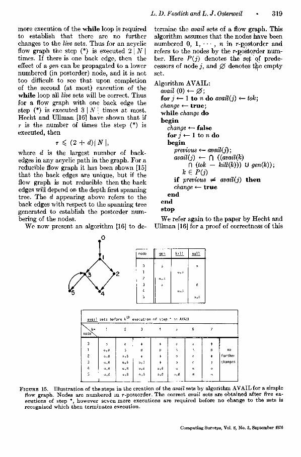
termine the avail sets of a flow graph. This algorithm assumes that the nodes have been numbered 0, 1, . . . , n in r-postorder and refers to the nodes by the r-postorder number. Here P ( j ) denotes the" se$ ~qf predecessors of node j, and ~/denotes the empty set.

Algorithm AVAIL: avail (0) <-- $2~; f o r j *-- 1 to n do avail(j) (--- tok; change <---- t rue; while change do b e g i n

change <---- false for j ~-- 1 to n do begin

previous <-- avail(j); avail(j) <--- N ((avail(k)

N (tok -- kill(k))) U gen(k)); k C P( j )

i f previous ~ avail(j) t hen change <-- t rue

end e n d s top

We refer again to the paper by Hecht and Ullman [16] for a proof of correctness of this

node 9en k111 nu l l

l a,t~

2 a,~

3 a B

4 ~,~

S a,(~

aval l sets before k th executlon of step + ~n AVAIL

nod•e k-- I 2 3 4 ~ 6 7

1 ~,B B B B B ~ B

2 a,B a,B @ @ ¢ ¢ ¢

3 a,B a,B ~,B ¢ ¢ ¢

4 ~,B e,B a,B a,B ~ ~

no

further

changes

FIGURE 15. I l lustrat ion of the steps in the creation of the avail sets by algori thm AVAIL for a simple flow graph. Nodes arc numbered m r-postorder . The correct avail sets are obtained after five executions of step *, however seven more executions are required before no change to the sets is recognized which then terminates execution.



algorithm. Its operation is illustrated in Figure 15 where the avail sets are indicated before each execution of the step labeled by (*). Here, as with the example for LIVE it is easy to verify that step (*) is executed twelve times. With the exception of the entry node, which is treated separately, it does not matter in what order the remaining nodes are visited in the while loop so far as correctness is concerned, but it does matter for the execution time. Again, the back edges are a critical factor. With r and d as defined before, Hecht and Ullman [16] show that

r ~ ( 2 + d ) ( t N I -- 1).

Empirical evidence obtained by Knuth [25] leads Hecht and Ullman [16] to the conclusion that in practice one can expect d ~< 6 and on the average d ~ 2.75 for FORTRAN programs. However, it is to be noted that there are pathological situations, as shown in Figure 16, for which the execution time is much larger than these numbers indicate.

SEGMENTATION OF DATA FLOW

Normally a program consists of a main program and a number of subprograms or external procedures. This segmentation of

nl

n t FIGURE 16. P a t h o l o g i c a l s i t u a t i o n in w h i c h t h e

e x e c u t i o n t i m e for t h e a v a i l a b i l i t y a l g o r i t h m is u n u s u a l l y long . He re d = 1 N -- 13, r = (I N ] -- 1) 3 a s s u m i n g a s g e n ( n , ) a n d a ~ k i l l (n~) a n d is n o t in a n y o t h e r gen or ]:ill sets.

the program is a natural basis for the segmentation of the data flow analysis. Here we describe how this is done in such a way as to permit detection of data flow anomalies on paths which cross procedure boundaries. We will see that the system for doing this naturally includes the detection of data flow anomalies on paths which do not cross procedure boundaries. In this section we describe the identification and representation of the data flow, and in the next section we describe the detection of anomalous data flow.

We make several assumptions at the out- set. The first concerns aliasing, the use of different names to represent the same datum. In crossing a procedure boundary the name of a datum typically changes from the so-called actual name used in the invoking procedure to the so-called dummy name used in the invoked procedure. I t is assumed here that the aliases for a datum are known and that a single token identifier is used to represent them. Thus, in particular, in our notation for representing actions on a token a along some path p we use P(p; c~) even when p crosses a procedure boundary and the datum represented by is known by different names in the two procedures. The second assumption we make is that the procedures under consideration have a single entry and a single exit. We could permit multiple entries and multiple exits, but it would complicate the discussion without adding anything really important to it. While we will discuss the segments as if they were procedures, it will be obvious that the discussion applies equally well to any single-entry, single-exit segment of a program. Our most restrictive assumption is that the call graph for the program is acyclic. This excludes recursion. We will discuss this restriction later.

Let us consider a flow graph GF(N, E, no) in which some node invokes an external procedure, as illustrated in Figure 17. In order to analyze the data flow in Gp(N, E, no) it is necessary to know certain facts about the data flow in the invoked procedure. In particular we need to know enough about the data flow in the invoked procedure to be able to detect anomalous patterns in the

Computing Surveys, Vol. 8, No 3, September 1976

G F (N, E, n o )

) G~ (N'. E: no')

I

FIGURE 17. At node n in GF(N, E, no) an external procedure is invoked. The flow graph of the invoked procedure is represented by Gr' (N', E', no').

flow across the procedure boundaries. Re- ferring to GF in Figure 17 and considering a single token a, it becomes evident that we need to recognize three cases to detect anomalous patterns of the form purp' on paths crossing the procedure boundary:

P(--~n; ~) ~ pu + p', a) P(n; a) ~ rp -~ p';

b) P ( n ; a ) ~ pu + p', P(n--% a) ~ rp + p';

t c) P(--~n;a) -= pu + p , P(n; a) -~ 1 "t- p , P(n--*; c~) ~ rp -k p.

Thus all we need to know about the data flow in the invoked procedure is whether P(n; ~) has one of the following three forms: rp W p', pu Jr p', 1 W p'. The last form represents the situation in which there is at least one path through the invoked procedure on which no reference, no definition, and no undefinition of a takes place. I t is evident that a particular P(n; a) could have more than one of these forms, e.g., ru W 1 has all three forms. Similar consideration of the problem of detecting anomalous path expressions of the form pddp' and pdup' leads to the conclusion that the following additional forms for P(n; a) need to be recognized: dp ~ p', pd + p, up ~ p'.

We now wish to extend these ideas to


permit recognition of situations where an anomalous path expression exists on all paths entering or leaving a node. This recognition is important because it permits us to conclude something about the presence or absence of anomalous path expressions on executable paths. Figure 1 makes it clear tha t some paths in a flow graph may not be executable, and it is evident that anomalous path expressions on them are not important. Only anomalous path expressions on executable paths are important as indicators of a possible error. Unfortunately, the recognition of executable paths is difficult 2, but if we make the reasonable assumption that every node is on some executable path, then if all paths through a node are known to be anomalous we may draw the very useful conclusion that there is an anomalous expression on an executable path. Certain additional forms for path expressions need to be. distinguished to achieve this. We observe, for example, tha t if

P(---m; a) -- pu and P(n; a) -- rp',

then on every path in Gr of the form no, • • • , n, . . • there is an anomalous path expression purp'. Thus it would be desirable to be able to distinguish the form rp. Notice also that if

P(--*n;a) - p u , P ( n ; a ) - -rp ' + 1, P(n---% a) - rp,

then the same conclusion can be drawn, so it is also desirable to distinguish the form rp -4- 1. Similar considerations show the need for recognizing the forms pu, pu + 1, 1 and similar considerations for anomalous expressions of the form pddp', and pdup' lead to corresponding forms involving d and u.

Collecting these results leads to the seven forms for path expressions shown in Figure 18. Corresponding sets A~(n), B ~ ( n ) , . . . , I (n ) which are subsets of the token set are defined as follows:

a E A~(n) if P ( n ; a ) - xp; a EBb(n) if P ( n ; a ) = xp ~- 1;

a E I (n) if P ( n ; a ) = l (n ) .

= Indeed th is problem is not solvable in general, for if we could solve i t we could solve the ha l t ing problem [18].



label path expression

A xp x

B x xp+l

C X xp+p '

D x px

E x px+l

F px+p ' x

I l

FIOUI~B 18. Seven forms for path expression in single-entry, single-exit flow graphs and labels used to identify them. The parameter x stands for r, d, or u.

These sets are called path sets. Although this classification scheme was developed for situations in which n represents a procedure invocation as illustrated in Figure 17, it will be recognized that it applies when n is a simple node representing, say, an assignment statement• For example if n represents a ~-- a + # and tok ffi {a, #, ~}, then

a E Ar(n) , a E C,(n) fl E A~(n), E C,(n) a E Dd(n), a E Fd(n) E I (n ) .

In such simple cases membership in the sets can be determined by rather obvious rules. On the other hand, when the node represents a procedure invocation, determination of membership in the path sets requires an analysis of the data flow in the procedure. I t is this problem to which we now direct our attention.

Suppose the path sets for node n' are to be determined. We assume that n' represents the invocation of an external procedure with flow graph Gr and that the path sets for the nodes of Gr have been determined already. (Our focus of attention now shifts to the invoked procedure and to avoid an excess of primes we have switched the role of primed and unprimed quantities shown in Fig. 17.) We also assume that no data actions take place at the entry node and exit node of Gr ; thus

I(no) = tok and I(n~xit) -- tok.

This assumption is not restrictive since we

can augment Gr by attaching a new entry node and new exit node with these prop- erties without affecting the data flow patterns. The algorithms for determining the path sets are presented informally below. They are presented in alphabetic order; however, as will become apparent, a different order is required for their execution. A satisfactory execution order is A, (n ' ) , C~(n'), B~(n'), D~(r[), F~(n'), E , ( ~ ) , I (n ' ) . Algorithm Determine A x( n')

1) for all n such that n E N - {n.xit} do null(n) (--- I (n) U B~(n) ; kill(n) ~-- A~(n) ; gen(n) ~ tok

-- (kill(n) U null(n)) ; 2) null(n~it) (---- f2~;

kill(noxit) ~ ;~; gen( ne,,it) ¢--- tok;

3) execute LIVE on Gp ; 4) A,(n ' ) ~ tok - live(no) ;

{comment--the null sets are not explicitly needed but are included here for clarity}.

Algorithm Determine B~( n') 1) for all n such that n E N do

null(n) ~-- I (n) U B, (n) ; kill(n) (---- Ax(n) ; gen(n) *--- tok

- (kiU(n) U null(n) ) ; 2) execute LIVE on Gr ; 3) B~(n') ~ (tok - live(no))

[7 (tok - ' a , ( n ' ) ) fl C,(n') . • . !

Algorithm Determine C,( n ) 1) for all n such that n E N do

gen(n) ~ C~(n) ; kill(n) ~ (Av(n) U A , (n ) ) ;

{comment--x, y, z is any per- mutation of r, d, ul

null(n) ,,-- tok - (gen(n) U kill(n))"

2) execute LIVE on Gr ; 3) C~(n') ~ live(no).

Algorithm Determine D,( n') 1) for all n such that n E N do

gen(n) ~-- D,(n) ; kill(n) (---(F,(n) U F,(n)) ;

{comment--x, y, z is any per- mutation of r, d, u}

null(n) (-- tok


- (gen(n) U kil l(n)) ; 2) execute AVAIL on Gr ; 3) D~(n') ~-- avail(nox,t).

Algorithm Determine E,( n') 1) for all n such that n E N - {no} do

gen(n) ~-- D~(n) ; kill(n) (-- Fv(n) U F,(n) ;

{comment--x, y, z is any per- mutation of r, d, u}

null(n) (-- tok - (gen(n) U kill(n) ) ;

2) gen(no) (-- $ok; kill(no) ~- ~ ; null(no) ¢--- 25;

3) execute AVAIL; 4) E~(n') ~-- avail(n~xi,)

N (tok - D,(n ' ) ) N F,(n ' ) .

Algorithm Determine F,( n') 1) for all n such that n E N - {no} do

gen(n) (--- D~(n) U D,(n); {comment--x, y, z is any per-

mutation of r, d, u} kill(n) (--- F,(n) ; null(n) (-- tok

-- (kill(n) U gen(n) ) ; 2) gen(no) *--- tok;

kill(no) *--- ~ ; null(no) *-- 25;

3) execute AVAIL; 4) F,( n') ~-- tok - avail(ned,t)

Algorithm Determine I ( n') 1) I (n ' ) ~ N I (n ) .

h E N

Since LIVE and AVAIL terminate, it is obvious that these algorithms terminate. Proofs of correctness for some of these algorithms are presented below.

Proof Determination of A~(n') is correct Let a E tok. By step 4 of the algorithm a E A~(n') if and only if a ~ live(no). Take the "if" part first:

~ live(no) ~ P(no-*; a) # gp + p' P(n0--~; a) =--- kp or

P(no-*; a) --= kp + 1,

or P(no--% a) ------ 1. The last two alternatives are ruled out because by step 2 of the algorithm gen(n~,,t) = tok. Consequently, because of the construction of the k,ll sets in step 1, a ~ live(no) ~ P(n0-*; a)


=-- xp. We observe P(n'; a) ffi P(no; a) P(no-~; a) = P(no - , ; a ) , the last equal- ity following from the fact that no data action takes place at no. Thus a E live(no) =~ P(n'; a) == xp; i.e., a E A~(n'). Now consider the "only if" part.

a E live(no) ~ P(no--*; a) ------ gp + p' Consequently, because of the construction of the gen sets P (no~; a) -- yp + p' where y # x. (Note that a E gen(n) implies, by step 1, P(n; a) - x p , P(n; (~) - xp + 1, P(n; a) - 1).Con- sequently, a E live(no) ~ P(n'; a) -- yp + p' # xp; i.e., a ~ A~(n ' ) .~

Proof Determination of B , (n ' ) is correct Let a E tok. By step 3 of the algorithm o~ E B,(n ' ) if and only if a E live(no) and

A ~ ~ x(n ) and o~ E C,(n') Take the "if" part first: a ~ live(no) ~ P(no-o; a) = kp, orP(no--*; ~) = kp + 1, orP(no-o; a) = 1. The first and last alternatives are ex- cluded by the conditions a ~ A , (n ' ) and

t ot E C,(n ). This leaves only,P(no--*; a) = kp + 1 and using a E k i l l ( n ) P ( n ; a ) = xpgivesP(no---*;a) -- xp + 1. Finally

P(n'; a) = P(no; ~)P(no--*; ~) -~ P ( no---* ; a)

P(n'; a) -~ xp + 1;

i.e., a E B,(n ' ) . Now consider the "only if" part.

a E live(no) ~ P(no---~; a) = gp + p'.

From step 1 it is seen that

a E gen(n) ~ P ( n ; a ) - y p + p ' , y # x .

Hence a E live(no) ~ P(no-*; a) -- yp + p', y # x, and from this it is easily concluded that a ~ B,(n ' ) . It is immediately evident that a E A~(n') a E Bx(n') and that a ~ C~(n') ~ a E

t B , ( n ).[]

Proof Determination of D~(n') is correct Let a E tok. By step 3 of the algorithm

a E D~(n') if and only if a E avail(nex,O.

Take the "if" part first.

a E avail(ne,~it) ~ P(-~nex,t; a) - pg.

Computing Surveys, VoL 8, No. 3, September 1976


Hence

P(n ' ; a) -- P(-'-~nexlt; ~)P(nex,t; a) -- pg.

Now using the fact that a E gen(n) P(n; a) ffi px we conclude that

a E avail(nexit) ~ P(n ' ; a) - px; i.e., a E Dx(n') .

Now take the "only if" part.

a ~ avail(ne.it) ~ P(--~ne, it; a) -- pk T p' or P(-~ne~,t; a) --- 1.

Since a E kill(n) implies P(n; a) !

py ~ p , y ~ x, it easily follows that a ~ avail(n~z,t) ~ P(n ' ; a) ~ px; i.e.,

?

a ~ Dx(n ) . ~

The last item to be discussed in this section is the initiation and progressive determination of the path sets for a program. Consider the call graph shown in Figure 5. Since the subprogram FUNB invokes no other subprogram, the algorithms just presented are unnecessary in the determination of the path sets for the nodes of the flow graph representing FUNB. In this flow graph each node will represent a simple statement or part of a statement having no underlying structure, so the path set determination can be made by inspection. Once this is done the path sets for the nodes of the flow graph representing SUBA can be determined, since the path sets are known for the only subprogram it invokes. The same remarks apply to the flow graph representing FUNA. Finally, after these path sets are determined it is possible to determine the path sets for the nodes of the flow graph representing MAIN. Thus by working backwards through an acyclic call graph it is possible to apply the algorithms just described. We call this backward order the leafs-up subprogram processing order. We have restricted our attention to acyclic call graphs because this procedure breaks down if a cycle is present in the call graph. One way to solve this problem if cycles are present might be to carry out an iterative procedure, as suggested by Rosen [30], in which successive corrections are made to some initial assignment of path sets but we have not pursued this idea.

DETECTING ANOMALOUS PATH EXPRESSIONS

I t will be recalled that we have defined an anomalous path expression to have one of the

! f ? forms: purp, pddp, or pdup. Let us assume now that the path sets have been determined for every node of a flow graph G~,(N, E, no). I t should be evident that if (n, n') E E and a E Fu(n) and a E Cr(n'), then there is a path expression of the form purp': a E Fu(n) , a E Cr(n') =* P(nn ' ; a) - purp' -[- pip. Note, however, that the undefinition and reference do not necessarily occur on nodes n and n' respectively. In- deed, these data actions may not even occur on nodes of this flow graph: they might occur on nodes of other flow graphs representing invoked procedures. We only know that on some path which includes the edge (n, n') there is an anomalous path expression. Also this anomalous path expression may not be on an executable path, but if a E D~(n) and a E Ar(n ' ) , then we may reasonabl~" conclude that the path expression purp occurs on an executable path. In this case our assumptions imply that on every path which includes the edge (n, n') there must be an anomalous path expression:

E Du(n) , a E Ar(n') ~ P(nn ' ; a) ---- purp'. We assume at least one of these paths is executable. In this section these ideas are expanded to include the detection of anomalous path expressions on paths which go through a selected flow graph.

Assume that the path sets have been constructed for a flow graph Gp, and we wish to determine whether

P(n; a)P(n---*; a) =- pxyp' "~ pH

o r

P(n; a)P(n---~; a) -- pxyp'

for each n E N and each a E tok. For anomaly detection we are interested in those cases whenx = u , y - r o r x = d , y = d, or x = d, y = u, but there is no need to fix the values of x and y now. A similar, but not equivalent, pair of problems is to determine whether

P(-*n; a)P(n; a) ~- pxyp' -~- p"

o r

Compu t ing Surveys , Vol 8, No 3, September 1976


P(---~n; a)P(n ; a) - pxyp'

for each n E N and each a C tok. The discussion of the last section should make it apparent that the first pair of problems can be attacked with the algorithm LIVE and the second pair of problems can be attacked with the algorithm AVAIL. Indeed, the algorithms presented in the last section have, in effect, solved these problems.

Consider the algorithm to determine A~(n') . After execution of step 3, suppose we construct the sets

A~(n--~) = tok - live(n)

for all n E N. Note that in step 4 we did this for the entry node only. It is evident that a E Ax(n--~) implies P(n---~; a) = xp, and conversely. Hence if a E Dr(n) and a E A~(n---~) we know that

P(n; a)P(n---% a) ~-- pyxp'

and so if y = u and x = r, an anomalous path expression of the form purp' is known to be present.

Now, using the idea and notation suggested in the last paragraph assume that we augment the last step in the algorithm for A~(n') , C~(n'), D~(n'), and F~(n') described in the last section to construct the sets A~(n--~), C~(n---~), D~(----~n), F~(---*n). Using them we construct the set intersec- tions: F~(n) Iq C~(n--~), D~(n) rl A~(n.-o), F~(---*n) f'l C~(n), and D~(---~n) Iq Ay(n) . Then it is seen that:

a E Fx(n) fl C~(n---*) ¢:* P(n; a)P(n---*; a) - pxyp' q- p";

a E D~(n) Iq Ay(n---*) ¢=* P(n; a)P(n--*; a) - pxyp';

,~ E F~(--,n) N C~(n) ¢=* P(--m; a ) P ( n ; a) -- pxyp' q- p";

a E D~(--m) fl A~(n) ¢=* P(---m; a)P(n ; a) - pxyp'.

The proofs of these assertions, which we omit, are essentially the same as those given in the previous section, Segmentation of Data Flow, for the determination of the sets A~(n') , . . . .

It will be recognized that the segmentation scheme described in the previous section permits exposure only of the first and

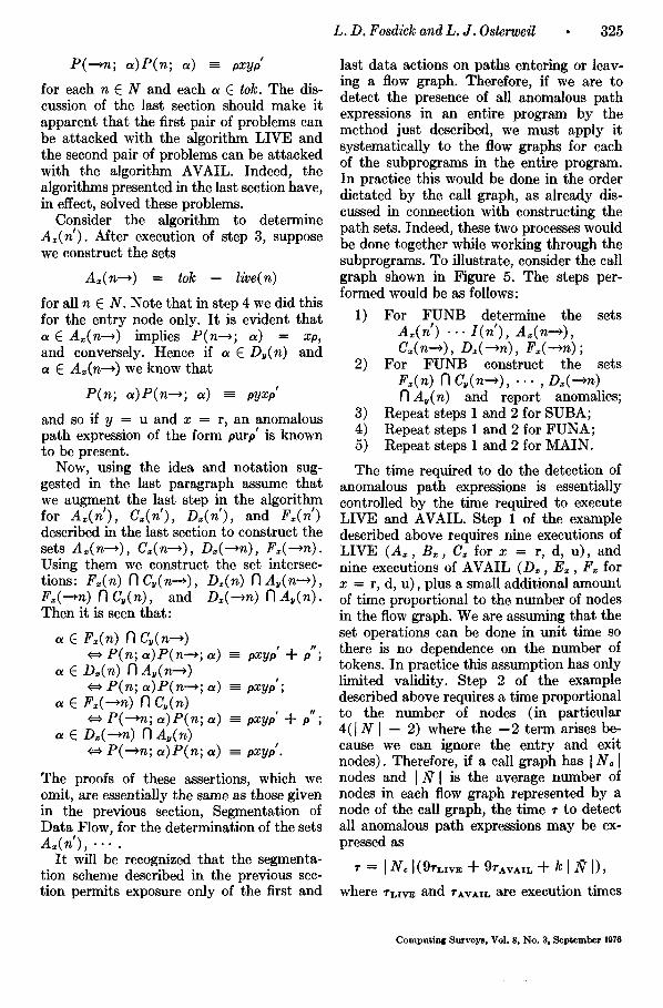
last data actions on paths entering or leaving a flow graph. Therefore, if we are to detect the presence of all anomalous path expressions in an entire program by the method just described, we must apply it systematically to the flow graphs for each of the subprograms in the entire program. In practice this would be done in the order dictated by the call graph, as already discussed in connection with constructing the path sets. Indeed, these two processes would be done together while working through the subprograms. To illustrate, consider the call graph shown in Figure 5. The steps performed would be as follows:

1) For FUNB determine the sets Ax(n') . . . I ( n ' ) , Ax(n--~), Cx(n-*), D~(-,n), F~(--m);

2) For FUNB construct the sets F~(n) N Cy(n--~), . . . , D~(---m) N A y ( n ) and report anomalies;

3) Repeat steps 1 and 2 for SUBA; 4) Repeat steps 1 and 2 for FUNA; 5) Repeat steps 1 and 2 for MAIN.

The time required to do the detection of anomalous path expressions is essentially controlled by the time required to execute LIVE and AVAIL. Step 1 of the example described above requires nine executions of LIVE (A~, B~, C~ for x -- r, d, u), and nine executions of AVAIL (D~, E~, F~ for x = r, d, u), plus a small additional amount of time proportional to the number of nodes in the flow graph. We are assuming that the set operations can be done in unit time so there is no dependence on the number of tokens. In practice this assumption has only limited validity. Step 2 of the example described above requires a time proportional to the number of nodes (in particular 4( I N ] - 2) where the - 2 term arises because we can ignore the entry and exit nodes). Therefore, if a call graph has I N. I nodes and I~1 is the average number of nodes in each flow graph represented by a node of the call graph, the time • to detect all anomalous path expressions may be ex- pressed as

r -- IN, 1(9r,.,w + 9rAvAIL + k I h7 I),

where rL~v~ and rxvxm are execution times

Computing Surveys, Vol. 8, No. 3. September 1976


for LIVE and AVAIL. If we use the results given in the section Algorithms to Solve the Live Variable Problem and the Availability Problem for the execution times for LIVE and AVAIL, we see that in practical situations we can expect to detect the presence of all anomalous path expressions in a program in a time which is proportional to the total number of flow graph nodes. While the constants of proportionality might be large and there would be a substantial over- head to create the required data structures, the important point is that a combinatorially explosive dependence on IN I has been avoided.

The principal reason why a combinatorial explosion has been avoided is that we have not looked explicitly at all paths. The loss of information resulting from this does not prevent us from detecting the presence of anomalous path expressions, but it greatly restricts our knowledge about specific paths on which the anomalous path expression occurs. Thus if a E Fu(n)N Cr(n--,), we know that on some path starting at n we will find an expression of the form purp', but we do not know which path and we do not know which nodes on the path contain the actions u and r on a. This problem can be attacked directly by performing a search over paths starting at node n. This search can be made quite efficient if we deal with one token at a time. The idea is to use a depth first search but to restrict it so that we avoid visiting any node n' such that a ~ C~(n'--*). While this strategy does not preclude backtracking, it tends to reduce it and generally restricts the number of nodes visited in the search. It seems certain that more efficient schemes for localizing the anomalous path expression can be constructed.

The information gathered for the detection of anomalous path expressions is valuable for other purposes. For example, it determines which arguments need initialization before execution of a procedure--thus it could be used to supply this information as a form of automatic documentation. Al- ternatively, this information can be used to verify assertions by the programmer con- cerning arguments needing initialization.

Similarly, it is possible to determine the arguments which are assigned values by a procedure, i.e., the output arguments. How- ever, unlike the case for initialization where the set Cr(n t) identifies the arguments re- quiring initialization, none of the path sets is sufficient for this purpose. Notice in particular that Fd(n ) is not satisfactory because P(n'; a) - pdr obviously implies that a is an output for the procedure represented by n' yet a ~ Fd(n'). However, it is not difficult to construct an algorithm for this purpose. Indeed, we only need to modify one step in the algorithm for Fx(n'); in particular, replace gen(n) (-- Dr(n) (J D~(n) by gen(n) (---- Du(n).

Then after step 4, a E Fd(n') implies a is an output for the procedure represented by n'. I t will be recognized that this excludes tokens for which P(n'; ~) =- pdr*u. This is reasonable, since the definition is destroyed by the subsequent undefinition, and no value is actually returned to the invoking procedure. Thus we have a mechanism for providing automatic documentation about procedure outputs, or for verifying assertions about which procedure arguments are output arguments.

CONCLUSION

As noted in an earlier section of this paper, we have implemented a FORTRAN program analysis system which embodies many of the ideas presented here. This system, called DAVE, [27, 28] separates program variables into classes that are somewhat similar to those shown in Figure 18. DAVE also detects all data flow anomalies of type purp' and most of the data flow anomalies of types pddp' and pdup'. DAVE carries out this analysis by performing a flow graph search for each variable in a given unit, and analyz- ing subprograms in a leafs-up order, which assures that no subprogram invocation will be considered until the invoked subprogram has been completely analyzed. An improved version of DAvE would continue to analyze the subprograms of a program in leafs-up order, but would use the highly efficient, parallel algorithms described here to either detect or disprove the presence of data flow

Computing Surveys. VoL 8, No 3, September 1976

anomalies. The variable-by-variable depth first search currently used in DAv~ exclu- sively, would be used only to generate a specific anomaly bearing path, once the more efficient algorithms had shown that an anomaly was present. Such a system would have considerably improved efficiency characteristics and, perhaps more important, could be readily incorporated into many existing compilers which already do live variable and availability analysis in order to perform global optimization.

The apparent ease with which our anomaly detection scheme could be efficiently integrated into existing optimizing compilers is a highly attractive feature and a strong argument for taking this approach. Other methods for carrying out anomaly detection can be constructed, but most that we have studied lack efficiency and compatibility with existing compilation systems. One such method, which is quite interesting for its strong intuitive appeal, involves symbolic execution of the program. Symbolic execution, a powerful technique which has recently found applications in debugging, program verification, and validation [8, 19, 22], involves determining the value of each program variable at every node of a flow graph as a symbolic formula whose only unknowns are the program's input values. These formulas of course depend upon the path taken to a given node. A notation similar to regular expression notation could be used to represent the set of symbolic expressions for a variable at a node, corresponding to the set of paths to the node. If these expressions were to be stored at their respective nodes, a flow graph searching procedure could be constructed which would be capable of detecting all the anomalies described here by careful examination of the way the expressions evolved along paths traversed by a single flow graph search. Moreover, because the symbolic execution carried along far more information than does our proposed system, even more powerful diagnostic results are possible.

The relative weaknesses of such a method are its lack of efficiency and the difficulty of incorporating it into existing compiling systems. Although it seems reasonable to


suppose that sophisticated representation schemes could be used to reduce the very large time and space requirements of the symbolic execution system, it also seems clear to us that even such reduced requirements would necessarily greatly exceed those of our proposed system. We have finally concluded that symbolic execution systems currently seem more attractive" as stand alone diagnostic systems where their greater level of detail can be used to carry out more extensive program analysis, but at greater cost. We believe, moreover, that our proposed data flow analysis scheme can and should be integrated into compilers in order to provide highly useful error diagnosis at small additional cost. The diagnostic output of a system such as ours would then be useful input to a symbolic execution system.

Much has been learned from our experiences with the current version of DAVE. Believing that similar systems should be used in state-of-the-art compilers, we now summarize these experiences in order to place in better perspective the problems and benefits to be expected.

Certain programming practices and constructs which are present in FORTRAN and common to a number of other languages cause difficulties for data flow analysis systems such as DAVE. The handling of arrays, as mentioned earlier, is one such example. Problems arise when different elements of the same array are used in in- herently different ways and hence have different patterns of reference, definition, and undefinition. Static data flow analysis systems such as DAVE are incapable of evaluating subscript expressions and hence cannot determine which array element is being referenced by a given subscript expression. Thus, as stated earlier, in DAVE and in many other program analysis systems arrays are treated as though they were simple variables. This avoids the problem of being unable to evaluate subscript expressions, but often causes a weakening or blurring of analytic results. As an example, consider the program shown in Figure 19. Suppose n t is the node of GMAIN(N, E, no), the flow graph of the main program, which invokes SQUARE. Denote by R( . , 1) and

Computing Surveys, Vol, 8, No, 3, September 1976


DIMENSION R(lO0,2)

READ(5,10)(R(I,]),I:I,]O0)

10 FORMAT(FIO.2)

CALL SQUARE(R)

WRITE(6,20)(R(I,2),I=I,IO0)

20 FORMAT(IX,FIO.2)

STOP

END

SUBROUTINE SQUARE(R)

DIMENSION R(IO0,2)

DO I0 I=I , I00

I0 R(I , I )=R(I ,2)**2

RETURN

END

FIGURE 19. A program in which failure to dis- t inguish between the differing pa t t e rn s of reference, definit ion and undef ini t ion of differ- en t array elements prevents the detection of d a t a flow anomalies .

R(. , 2) arbitrary elements of column 1 and column 2 respectively of array R. Now clearly R( . , 1) E Ad(n') and R( . , 2) E A,(n'). In addition, it is clear that R( . , 1) E Dd(--*n ~) and R(-, 2) E Du(-*n'). Hence P(-m'; R(., 1))P(n'; R(., 1)) -- pddp', and P(-~n'; R(., 2))P(n'; R(., 2)) ---

!

purp, and we see there are two data flow anomalies present. DAVE, however, treats R as a simple variable and determines that R E Ad(n'), R E Dd(n'), R E Dd(---~n')

, I andR E A,(n--*). Thus P(---*n ;R)P(n';R) - pdrp' and P(n'; R)P(n'---~; R) - - p d r p ,

and no data flow anomalies will be detected. This loss of anomaly detection power is worrisome, and it is seemingly avoided only when programmers call functionally distinct subarrays by separate names.

There are also certain difficulties involved in determining the leafs-up subprogram processing order referred to earlier. This order is important, because it ensures that each subprogram will be analyzed exactly once, yet that data flow anomalies across subprogram boundaries will be detected. If subprogram names are passed as argu-

ments, this order may become difficult to determine. This difficulty can arise because the name used in a subprogram invocation may not be the name of a subprogram, but rather can be a variable which has received the subprogram name, perhaps through a long chain of subprogram invocations. All such chains must be explored in order to expose all subprogram invocations and then determine the leafs-up order. Recent work by Kallal and Osterweil [20] indicates that the AVAIL algorithm can be used to efficiently expose all such invocations.

Recursive subprograms pose another ob- stacle to determining leafs-up order. Al- though recursion is not allowed in FORTRAN, it is a capability of many other languages. Moreover, it is possible to write two FORTRAN subprograms such that each may invoke the other, but such that no program execution will force a recursive calling sequence. Such a program would be legal in FORTRAN, but would not appear to have sufficient leaf subprograms (i.e., those that invoke no others) to allow construction of the complete leafs-up order. This problem is not adequately handled by DAVE, however no FORTRAN programs with this construction have been encountered. In any case current work indicates that recursive programs can be analyzed using the methods described here.

Finally it should be observed that subprogram invocations involving the passing of a single variable as an argument more than once may be incorrectly analyzed. This occurs because DAVE assumes that all subprogram parameters represent different variables as it analyzes subprograms in leafs-up order.

Despite these limitations, the DAvE system has proven to be a useful diagnostic tool. We have used DAVE to analyze a number of operational programs and it has often found errors or stylistic short- comings. Among the most common of these have been: variables having path expressions equivalent to purp' (referencing uninitialized variables), and pdup' (failing to use a computed value) occurring simul- taneously, usually due to a misspelling; subprogram parameters having path ex-

Computing Surveys, Vol. 8, No 3, September 1976

pressions equivalent to 1, caused by naming unused parameters in parameter lists; and C O M M O N variables ha,ving pa th expressions equivalent to purp or pdup' usually due to omitting C O M M O N declarations from higher level program units.

The cost of using DAv~. has proven to be relatively high, par t ly due to the fact tha t it is a pro to type built for flexibility, and not speed, and par t ly due to the failure to use the more efficient algorithms described here. We have observed the execution speed of the system to average between 0.3 and 0.5 seconds per source s ta tement on the CDC 6400 computer for programs whose size ranged from several dozen to several thou- sand statements. The total cost per statement has averaged between 7 and 9 cents per s ta tement for these test programs using the Universi ty of Colorado Comput ing Center charge algorithm. I t is, of course, anticipated tha t these costs would decline sharply if a production version of DAvE were to be implemented.

Based on these experiences and observa- tions, we believe tha t systems like DAvE can serve the impor tant purpose of auto- matically performing a thorough initial scan for the presence of certain types of errors. I t seems tha t the most useful characteristics of such systems are tha t 1) they require no human intervention or guidance and 2) they are capable of scanning all paths for possible da ta flow anomalies. A human tester need not be concerned with designing test cases for this system, yet can be assured by the system tha t no anomalies are present. In case an anomaly is present, the system will so advise the tester and further testing or debugging would be necessary. Clearly such a system is capable of detecting only a limited class of errors. Hence further testing would always be necessary. Through the use of a system such as DAVE, however, the thrust of this testing can be more sharply focussed. I t seems tha t these systems could be most profitably employed in the early phases of a testing regimen (e.g., as par t of a compiler) and used to guide and direct later testing efforts involving more powerful systems tha t employ such techniques as symbolic execution. Towards this end, fur-


ther work should be done to widen the class of errors detectable by means such as those described in this paper.

ACKNOWLEDGMENTS We want to close with a grateful recognition of the stimulating and valuable discussions we have had on this subject with our colleagues and students--especially Jim Boyle, Lori Clarke, Hal Gabow, Shachindra Maheshwari, Carol Miesse, and Paul Zeiger--and the helpful comments of the referees. Finally, we gratefully acknowledge the financial assistance provided by the National Science Foundation in this work.

REFERENCES

[1] A~o, A. V.; ANn ULLMAN, J. D. "Node listings for reducible flow graphs," in Proc. of the 7th Annual ACM Symposium on Theory of Computing, 1975, ACM, New York, 1975, pp. 177-185.

[2] ALLEN, F .E . "Program optimization," in Annual Review in Automatic Programming, Pergamon Press, New York, 1969, pp. 239- 307.

[3] ALLEN, F.E. "A basis for program optimi- z ation," in Proc. IFIP Congress 1971, North- Holland Publ. Co., Amsterdam, The Nether- lands, 1972, pp. 385-390.

[4] ALLEN, F. E.; AND COCKE, J. Graph- theoretzc constructs for program control flow analyszs, IBM Research Report RC3923, T. J. Watson Research Center, Yorktown Heights, New York, 1972.

[5] ALLEN, F. E. "Interprocedural data flow analysis," in Proc. IFIP Congress 1974, North Holland Publ. Co., Amsterdam, The Netherlands, 1974, pp. 398-402.

[6] ALLEN, F. E.; AND COCKE, J. "A program Comm

[7] BALZEa, R. M. "EXDAMS: Extendable debugging and monitoring system," in Proc. AFIPS 1969 Spring Jr. Computer Conf., Vol. 34, AFIPS Press, Montvale, N.J., 1969, pp. 567-580.

[8] CLARKE, L. A system to generate test data and symbolically execute programs, Dept. of Computer Science Technical Report $Cu- CS-060-75, Univ. of Colorado, Boulder, 1975.

[9] DENNIS, J .B. "First version of a data flow procedure language," in Lecture notes ~n computer science 19, G. Goos and J. Hart- manis (Eds.), Springer-Verlag, New York, 1974, pp. 241-271.

[10] FAmLE~C, R.E. "An experimental program testing facility," in Proc. First National Conf. on Software Engineering, 1975, IEEE $75CH0992-8C, IEEE, New York, 1975, pp. 47-55.

[11] GOLDSTINE, H. H . ; AND VON NEUMANN, J . Planning and coding problems for an elec- tronic computing instrument," in John yon Neumann, collected works, A. H. Taub (Ed.),

Computing Surveys, V~I. 8, No. 3, September 1976

330 • Data Flow Ana ly s i s I n Software Reliabil i ty

Pergamon Press, London, England, 1963, pp. 80-235.

[12] HABERMANN, A.N. Path expressions, Dept. of Computer Science Technical Report, Carnegie-Mellon Univ., Pittsburgh, Pa., 1975.

[13] HARARY, F. Graph theory, Addison-Wesley Publ. Co., Reading, Mass., 1969.

[14] HECHT, M. S.; AND ULLMAN, J. D. "Flow graph reducibility," SIAM J. Computing 1, (1972), 188-202.

[15] HECHT, M. S.; ANn ULLMAN, J . D . "Char- acterizations of reducible flow graphs," J. ACM 21, 3 (July 1974), 367-375.

[16] HECHT, M. S.; AND ULLMAN, J. D. "A simple algorithm for global data flow analysis problems," SIAM J. Computing 4 (Dec. 1975), 519-532.

[17] HOPCROFT, J.; AND TARJAN, R. E. "Effi- cient algorithms for graph manipulation," Comm. ACM 16 (June 1973), 372-378.

[18] HOPCROFT, J. E.; AND ULLMAN, J . D . For- mal languages and their relation to automata, Addison Wesley Publ. Co., Reading, Mass., 1969.

[19] HOWDEN, W . E . "Automatic case analysis of programs," in Proc. Computer Science and Statistics: 8th Annual Symposium on the Interface, 1975, pp. 347-352.

[29] KALLAL, V.; AND OSTERWEIL, L. J. Con- structing flowgraphs for assembly language programs, Dept. of Computer Science Tech- nical Report Univ. of Colorado, Boulder, (to appear 1976).

[21] KARP, R.M. "A note on the application of graph theory to digital computer programming," Information and Control 3 (1960), 179-190.

[22] KINo, J. C. "A new approach to program testing," in Proc. Internatl. Conf. on Re- liable Software, 1975, IEEE ~75CH0940- 7CSR, IEEE, New York, 1975, pp. 228-233.

[23] KENNEDY, K.W. "Node listings applied to data flow analysis," in Proc. of 2nd ACM Symposium on Pmncipals of Programming Languages, 1975, ACM, New York, 1975, pp. 10-21.

[24] KNU~H,D. E. The art of computer programming, Vol. I fundamental algorithms, (2d Ed.), Addison Wesley Publ. Co., Reading, Mass., 1973.

[25] KNUTH, D. E. An empirical study of FORTRAN programs, Software--Practice and Experience 1, 2 (1971), 105-134.

[26] MILLER, E. F., JR. RXVP, FORTRAN automated verificatwn system, Program Vali- dation Project, General Research Corp., Santa Barbara, Calif., 1974, pp. 4.

[27] OSTERWEIL, L. J.; AND FOSDICK, L D. "DAVE--a FORTRAN program analysis system," in Proc. Computer Science and Statistics: 8th Annual Symposium on the Interface, 1975, pp. 329-335.

[28] OSTERWEIL, L. J.; AND FOSDICK, L. D.. "DAVE--a validation, error detection and documentation system for FORTRAN programs," Software--Practice and Experience (to appear 1976).

[29] RODRIGUEZ, J. D. A graph model for parallel computatwn, Report MAC-TR-64, Project MAC, MIT, Cambridge, Mass., 1969.

[30] ROSEN, B. Data flow analysis for recurszve P L / I programs, IBM Research Report RC5211, T. J. Watson Research Center, Yorktown Heights, New York, 1975.

[31] SCHAEFFER, M. A mathematzcal theory of global program optimization, Prentice-Hall Inc., Englewood Cliffs, N. J., 1973.

[32] STUCKI, L. G. "Automatic generation of self-metric software," in Proc. IEEE Sym- posium on Computer Software Reliabdity, 1973, IEEE $73CH0741-9CSR, IEEE, New York, 1973, pp. 94-100.

[33] TARJAN, R. E. "Depth-first search and linear graph algorithms," SIAM J. Comput- ing (Sept. 1972), 146-160.

[34] TARJAN, R. E. "Testing flow graph reducibility," J. Computer and System Sciences 9, 3 (Dec. 1974), 355-365.

[35] ULLMAN, J. D. "Fast algorithms for the ehmination of common subexpressions," Acta Informatiea 2 (1973), 191-213.


Documents

Data Flow Analysis In Software Reliability* LLOYD D. FOSDICK and LEON J. OSTERWEIL