Data-Driven Contextual Modeling for 3D Scene Understanding

Yifei Shia, Pinxin Longc, Kai Xua,c,∗, Hui Huangb,c, Yueshan Xionga

aHPCL, National University of Defense TechnologybShenzhen University

cShenzhen VisuCA Key Lab / SIAT

Abstract

The recent development of fast depth map fusion technique enables the realtime, detailed scene reconstruction usingcommodity depth camera, making the indoor scene understanding more possible than ever. To address the specificchallenges in object analysis at subscene level, this work proposes a data-driven approach to modeling contextual in-formation covering both intra-object part relations and inter-object object layouts. Our method combines the detectionof individual objects and object groups within the same framework, enabling contextual analysis without knowing theobjects in the scene a priori. The key idea is that while contextual information could benefit the detection of eitherindividual objects or object groups, both can contribute to object extraction when objects are unknown.

Our method starts with a robust segmentation and partitions a subscene into segments, each of which represents eitheran independent object or a part of some object. A set of classifiers are trained for both individual objects and objectgroups, using a database of 3D scene models. We employ the multiple kernel learning (MKL) to learn per-categoryoptimized classifiers for objects and object groups. Finally, we perform a graph matching to extract objects using theclassifiers, thus grouping the segments into either an object or an object group. The output is an object-level labeledsegmentation of the input subscene. Experiments demonstrate that the unified contextual analysis framework achievesrobust object detection and recognition over cluttered subscenes.

Keywords: Scene understanding, object recognition, contextual modeling, data-driven approach

∗Corresponding author: kaixu@nudt.edu.cn

(a)

(b)

monitor

keyboard

mouse

cup

lamp

globe

cylinder

Figure 1: Scene understanding by our method. (a): Theinput point cloud of a table-top scene. (b): The labelingresult (legends show semantic labels in color).

1. Introduction1

With the rapid development of 3D sensing techniques,2

the digitalization of large-scale indoor scenes has be-3

come unprecedentedly accessible to a wide range of4

applications. Among the most exciting and promising5

applications, robot-operated exploration and interaction6

over unknown indoor environment would benefit signif-7

icantly from the availability of high-quality and realtime8

acquired 3D geometry information [1]. Such 3D in-9

formation can not only improve robot navigation and10

exploration, but more importantly, facilitate efficient11

robot-scene interaction with fine-grained understanding12

of scene objects. The latter may support highly complex13

robot tasks such as room cleaning.14

Motivated by the high demand, extensive research has15

been devoted to the understanding of scanned indoor16

scenes. Most existing works on scene understanding17

focus on large-scale objects, such as furniture, as well18

as their spatial layout [2, 3, 4, 5, 6], since the analysis19

Preprint submitted to Computers & Graphics November 16, 2015

is usually limited by the quality and resolution of input20

scans. Recent advances in volumetric scan fusion tech-21

nique (such as KinectFusion [7]) has made it possible22

to reconstruct quality and detailed scenes from scans23

captured by commodity depth camera (e.g. Microsoft24

Kinect and Asus Xtion). The dense point clouds pro-25

cessed by KinectFusion can well capture small scale ob-26

jects such as household objects, which enables detailed27

understanding at a subscene level, e.g. many objects28

placed a tabletop; see Figure 1.29

Object analysis at subscene level is arguably much more30

challenging than that at whole scene level. Firstly, un-31

like furnitures which are usually sparsely distributed in32

an indoor scene, household objects are often highly clut-33

tered due to the limited space of supporting surfaces [8].34

For example, a tabletop scene is typically cluttered with35

many on-table objects. Secondly, repetition of objects,36

which is ubiquitous among furnitures and has been ex-37

tensively exploited in previous works [3, 5], may not be38

as commonly seen among household objects. For ex-39

ample, the objects placed on a table are mostly unique40

within the subscene. Thirdly, from the acquisition point41

of view, smaller objects are often more sensitive to scan-42

ning imperfection. These challenges make the existing43

methods, dealing with large-scale furniture layout, un-44

suitable for the object analysis of small-scale subscenes.45

To address these challenges, it seems a natural option46

is to fully utilize the inter-object relations, or contextual47

information. However, a key prerequisite for contextual48

scene analysis is that all objects are segmented and la-49

beled with semantic tags [9], which is apparently infea-50

sible for an unsegmented scene. Essentially, context is51

defined with objects. Without knowing objects, how can52

we utilize contextual information to help the identifica-53

tion of objects? In this work, we try to tackle this prob-54

lem through integrating the discovery of both individ-55

ual objects and object groups into a unified framework.56

While the former involves grouping parts into an object,57

which detects individual objects, the latter amounts to58

finding structure groups [10] composed of multiple ob-59

jects, which can actually enhance or reinforce the de-60

tection and recognition of objects within the structure61

group. The key idea is that contextual information could62

benefit the detection of either individual objects or ob-63

ject groups, when objects are unknown. However, both64

can contribute to object extraction.65

To enable such unified framework, we take a data-driven66

approach equipped with several key procedures. First,67

we propose a robust segmentation method to partition a68

indoor scene into segments which each represents either69

an independent object or a part of some object. We then70

train a set of classifiers for both individual objects and71

object groups, based on a database of 3D scene models.72

To improve the classification accuracy, we employ mul-73

tiple kernel learning (MKL) [11] to learn per-category74

optimized SVM classifiers for various objects and ob-75

ject groups. Finally, we perform a graph matching to76

extract objects using the classifiers, thus grouping the77

segments into either an object or an object group. The78

input of our algorithm is an indoor scene point cloud,79

and the output is an object-level labeled segmentation80

of the input scene. Experiments demonstrate the ro-81

bust performance for both segment extraction and object82

recognition on several subscenes.83

Our approach possesses two key features compared with84

previous methods. First, we perform a segmentation85

process before recognition, which leads to robust han-86

dling of cluttered scenes. Second, instead of solving the87

recognition of individual objects and object groups as88

two separate problems, we encode features of both indi-89

vidual objects and object layout into a unified classifier90

via contextual modeling.91

2. Related Work92

Scene understanding is a long-standing research topic93

which has received extensive research from both com-94

puter vision and computer graphics community. We95

mainly review those works which take 3D point clouds96

as input.97

Point cloud segmentation. Mesh segmentation is a fun-98

damental shape analysis problem in computer graphics,99

for which both heuristic methods [12] and data-driven100

approach [13] have been extensively studied over the101

years. On the other hand, the segmentation of 3D point102

clouds remains to be a challenging problem.103

There are three kinds of methods for point cloud seg-104

mentation [14]. The first type is based on primitive105

fitting [3, 15, 5]. It is hard for these methods to deal106

with objects with complex shape. The second kind107

of techniques is the region growing method. Nan et108

al. [2] propose a controlled region growing process109

which searches for meaningful objects in the scene by110

accumulating surface patches with high classification111

likelihood. Berner et al. [16] detect symmetric regions112

using region growing. Another line of methods formu-113

lates the point cloud segmentation as a Markov Ran-114

dom Field (MRF) or Conditional Random Field (CRF)115

2

Over-SegmentationTraining

Testing

Segment Detection Object Recognition

Segment Generation

Plane Extractionclassifier1 classifier2 classifier3 classifier4

……

Segment Graph

Figure 2: An overview of our algorithm. We first over-segment the scene and extract the supporting plane on the patchgraph, then segment the scene into segments and represent the whole scene using a segment graph (a). To obtain thecontextual information, we train a set of classifiers for both single objects and object groups using multiple kernellearning (b). The classifiers are used to group the segments into objects or object groups (c).

problem [4, 17, 14]. A representative random field seg-116

mentation method is the min-cut algorithm [17]. The117

method extracts foreground from background through118

building a KNN graph over which min-cut is performed.119

The shortcoming of min-cut algorithm is that the se-120

lection of seed points relies on human interaction. We121

extend the min-cut algorithm by first generating a set122

of object hypotheses via multiple binary min-cuts and123

then selecting the most probable ones based on a voting124

scheme, thus avoiding the seed selection.125

Object recognition. Recently, the development of com-126

modity RGB-D cameras has opened many new oppor-127

tunities for 3D object recognition and scene recogni-128

tion [18, 19]. With the ever-growing amount of 3D mod-129

els becoming available, data-driven approach starts to130

play an important role in 3D object recognition and has131

gained great success [20].132

Nan et al. [2] propose a search-classify approach to133

scene understanding by interleaving segmentation and134

classification in an iterative process. Li et al. [6] propose135

scene reconstruction by retrieving objects from a 3D136

model database. Song et al. [21] render database mod-137

els from hundreds of viewpoints and train an exemplar-138

SVM classifier for each of them to achieve object recog-139

nition. Their method overcomes several difficulties in140

object recognition, such as the variations of texture, il-141

lumination, etc. Chen et al. [22] utilize contextual infor-142

mation for indoor scene understanding. Small objects143

and incomplete scans can be recognized with the help of144

contextual relationships learned from database objects.145

Our method lends itself to cluttered indoor scene anal-146

ysis through integrating segmentation and recognition147

into a single framework, which leads to a better per-148

formance when dealing with close-by objects than the149

contour-based method of [22].150

Another line of analysis method is unsupervised learn-151

ing based on the presence of repetitions or symmetries152

in indoor scenes [3, 5, 23]. A limitation of such ap-153

proaches is that such repetitive patterns are less com-154

mon in subscenes dominated by household objects, e.g.,155

a tabletop scene.156

Plane extraction. Plane extraction from point cloud is157

another important topic in scene understanding. For ex-158

ample, planes can be used to improve the reconstruc-159

tion of arbitrary objects containing both planar and non-160

planar regions [24].161

Perhaps the most widely used approach for plane extrac-162

tion is RANSAC based plane fitting [15]. This method163

scales well with respect to the size of the input point164

cloud and the number of planes. Mattausch et al. [5]165

utilize planar patches as a compact representation of the166

point cloud of an indoor scene, which facilitates effi-167

cient repetition detection in a large-scale scene point168

cloud. Zhang et al. [24] perform plane extraction to169

delineate non-planar objects. Plane extraction has also170

been performed in the analysis of RGB-D data [25, 26].171

These works trim the plane boundary and convert the172

input data into a compact polygonal representation. Re-173

cently, Monszpart et al. [27] propose to reconstruct the174

raw scan of man-made scenes into an arrangement of175

planes with both local fitting and global regularization.176

3

3. Overview177

The input of our algorithm is a 3D point cloud of indoor178

scene acquired and fused by KinectFusion. Our goal is179

to detect objects in the scene and recognize their seman-180

tic categories automatically. Our method proceeds in181

two stages. First, we segment the point cloud into seg-182

ments representing potential objects. Second, to achieve183

object extraction and recognition, we propose a joint es-184

timation of individual objects and object groups, as well185

as their semantic categories.186

Segment detection. In the first stage, we segment the187

input scene (Figure 2 (a)). Specifically, we first over-188

segment the entire scene and build a patch graph. We189

then extract the supporting plane with a method inte-190

grating RANSAC primitive fitting into graph-cut. Af-191

ter plane extraction, the remaining points are grouped192

into isolated groups. Within each group, we generate193

segments via a robust segmentation algorithm, which194

takes both geometry and appearance information into195

account. Based on the segmentation, we represent the196

entire scene as a segment graph with two types of edges197

representing direct spatial adjacency (solid lines in Fig-198

ure 2) and spatial proximity (dashed lines) between two199

segments, respectively.200

Object extraction and recognition. In the second phase,201

we extract objects via recognizing both individual ob-202

jects and object groups within a unified framework,203

based on the above segment graph representation.204

In an off-line stage, we train per-category optimized205

SVM classifiers with multiple kernel learning for both206

objects and object groups. The classifiers are trained207

using 3D database models. Each 3D model is first con-208

verted into 3D point cloud using virtual scanning and209

segmented using the method mentioned above. We then210

extract features from the corresponding segment graph211

and train classifiers based on the graph.212

In the online stage, we extract objects or object groups213

from the segment graph of the input scene, through214

searching for the subgraph matching corresponding to215

the occurrence of database objects and object groups.216

Once a matched subgraph is found, we use the cor-217

responding SVM classifier to estimate the probability218

of the match. Finally, we solve a labeling optimiza-219

tion which minimizes the overall matching cost for all220

matching probabilities.221

4. Segment detection222

Our goal is to partition the input scene into segments223

which each represents either an independent object or224

a part of an object. In order to segment objects from225

cluttered scenes, we propose an unsupervised segment226

detection approach to detect segments in 3D scene.227

Specifically, we first over-segment the input point cloud228

into a set of patches (Sec. 4.1) and detect the supporting229

plane (Sec. 4.2). We then group the remaining patches230

to extract potential objects or parts (Sec. 4.3) and rep-231

resent them as a segment graph (Sec. 4.4). See Algo-232

rithm 1 for an overview of our method.233

4.1. Patch graph generation234

We first over-segment the entire scene S into sev-235

eral patches, using the method in [28]. We build a236

patch graph based on the patches, denoted with Gp =237

(Vp,Ep), where Vp and Ep represent the patches and238

the near-by relations within the patches, respectively.239

Specifically, the near-by relations are determined by240

comparing the nearest distance between two patches241

with a threshold.242

Essentially, our segment detection algorithm is a graph-cut based approach. The most vital component forgraph-cut method is the definition of smooth term. Inthis section, the smooth terms for all graph-cut opti-mization are identical, which we first define here:

Es(xu, xv) = wc · Ec + wp · Ep + wn · En, (1)

where xu, xv are two adjacent patches. Ec, Ep, En are243

the differences between two adjacent patches in terms of244

color, planarity and normal. wc,wp,wn are the weights.245

Ec and Ep are computed based on the chi-square dis-tance of the color and planarity histogram between uand v, we normalize them to (0, 1). It is worth mention-ing that the planarity histogram are computed as fol-low: first compute the least-square plane for a patch,then built a histogram for distances of all points in thepatch to the plane. The formulation for En is differentfor convex and concave situations. Specifically, the for-mulation is:

En(xu, xv) = 1 − η(1 − cos θu,v), (2)

where θu,v is the angle between the average normals of246

patch Pu and Pv. For η, we take 0.01 (a small value) if247

the two adjacent patches form a convex dihedral angle248

4

Algorithm 1 :Segment Detection.

Input: scene SOutput: segment graph Gs

1: Gp ← OverSegment(S );2: S ← PlaneExtract(S ,Gp); //extract plane3: H ← SegHypGen(S ,Gp); //generate seg. hypo.4: T ← SegHypSelect(H); //select seg. hypo.5: Gs ← SegGraGen(T ); //generate seg. graph6: return Gs;

and 1 otherwise, to encourage cuts around a concave249

region [29].250

Our smooth term takes both geometry (planarity and251

normal) and appearance (color) factors into considera-252

tion, thus makes the patches belong to different objects253

can be detected easily.254

4.2. Supporting plane extraction255

Supporting plane is usually the largest object in most256

subscenes of an indoor scene, such as tables, beds,257

shelves, etc. The extraction of supporting plane is es-258

pecially useful since it makes the detection of objects259

on top of the supporting plane easier. Therefore, the260

first step of our segment generation is supporting plane261

extraction. For this task, perhaps the most straightfor-262

ward approach is RANSAC based primitive fitting [15].263

Since the objects placed on the supporting plane may be264

very small or thin, setting a hard threshold for point-to-265

plane distance may cause a lot of false positives. We266

therefore improve this method by adding a graph-cut267

optimization, to robustly segment on-top objects from268

the supporting plane.269

We try to assign each patch a binary label, denoted byX = [x1, . . . , xn] with xi ∈ {0, 1}. xi = 1 if patch Pi liesin the plane, and xi = 0 otherwise. We formulate thelabeling problem as graph cuts over the patch graph:

E(X) =∑u∈Vp

Ed(xu) +∑

(u,v)∈Ep

Es(xu, xv), (3)

where the data term is defined as:

Ed(xu) =

{δ, if xu = 1(1 − p

pmax) · (1 − d

dmax) · cos θu,l, if xu = 0

where δ is a constant value, d the distance between the270

center of u to the plane, and p the planarity of the patch.271

dmax and pmax is the maximum distance and planarity,272

respectively. We compute p as the average distance273

(a)

(b)

Figure 3: Plane extraction from the point cloud of atabletop scene by using our method (a) and RANSACbased primitive fitting (b), respectively. While ourmethod can segment out the supporting plane accu-rately, RANSAC missed some points due to the thin ob-jects.

of all the points in patch Pu to its corresponding least-274

square fitting plane. θu,l is the angle between the average275

normal of Pu and the normal of the plane.276

Figure 3 (a) demonstrates the segmentation results of277

our method. As a comparison, the RANSAC based278

primitive fitting can also get the majority of points cor-279

rectly, but it fails when dealing with small and thin ob-280

jects, as is shown in Figure 3 (b).281

4.3. Segment generation282

Segment hypothesis generation. After plane removal,283

object extraction only amounts to segmenting the iso-284

lated groups of patches on top of the supporting plane285

into individual objects. To solve the problem, we pro-286

pose to first generate a set of segment hypotheses and287

then select the most prominent ones based on a voting288

algorithm.289

We first update the patch graph Gp by removing the290

nodes belonging to the extracted plane. Based on the291

updated patch graph, we generate segment hypothe-292

ses by performing several times of binary graph cut,293

where the foreground corresponds to potential objects294

or prominent parts.295

Different from other graph cut method, we do not se-lect foreground seed heuristically. Instead, we use everypatch as seed and perform binary graph cuts for multiple

5

(b)

(a)

Figure 4: Illustration of our segment detection method.The scene is composed of two bottles stuck together on around table (a). We use every patch as seed to generatemany foreground hypotheses and then select the mostprominent ones (b).

times, generating many candidate foregrounds. In eachbinary cut, we select one patch as foreground seed butdo not prescribe any seed for background. This is per-formed by introducing a background penalty for eachnon-seed patch [30]. Specifically, we select one patch,denoted by Ps, labeling it as foreground xs = 1, andminimize over binary patch labels X = [x1, . . . , xn], xi ∈

{0, 1} (n is the number of patches) the following para-metric energy function:

Eλ(X) =∑u∈Vp

Eλd(xu) +

∑(u,v)∈Ep

Es(xu, xv), (4)

where the data term is defined as:

Eλd(xu) =

∞, if xu = 0 and u = s0, if xu = 1 and u = s0, if xu = 0 and u , sfu, if xu = 1 and u , s

fu =

{k(d(Ps, Pu) − λ), if d(Ps, Pu) > λ0, otherwise.

fu is the background penalty which penalizes a non-296

seed patch which is distant from the foreground seed.297

(a) (b)

Figure 5: Segment detection from the point cloud of ahighly cluttered scene (a) by using our method (b). Theinput data has a lot of close-by objects and the backview is not scanned, which makes the segmentation quitechallenging. Our method can segment out most objectsaccurately.

d(Ps, Pu) is the distance between the centers of patch Ps298

and Pu. We use k = 2.0 for a steep penalty to quickly299

reject those patches whose distance to Ps is larger than300

λ to be labeled as foreground. The parameter λ controls301

the range, centered around the foreground seed, within302

which one seeks for foreground patches. Instead of us-303

ing a hard threshold on this range, we slide λ from 0 to304

`d (the diagonal length of the bounding box of the entire305

scene) and find the first point where the total cut cost306

drops significantly (up to 50%) and take the resulting307

cuts as the segmentation result. The smooth term is the308

same as the one used for plane extraction in Eq. (1).309

Once we select every patch as seed and perform graph310

cut for each of them, we can obtain a set of foreground311

segments. To filter out the redundancy, we cluster312

the foreground segments using non-parametric mean-313

shift [31]. The similarity between two segments, de-314

noted as S and T , is measured by the Jaccard index, i.e.,315

s(S ,T ) = |S ∩ T |/|S ∪ T |. For example, as is shown316

in Figure 4 (b), selecting the seed patches in the same317

row will led to identical foregrounds, thus these fore-318

grounds will cluster together after the mean-shift pro-319

cessing, as the Jaccard index is high. For each cluster,320

we choose the cluster center as the segment hypothesis321

for that cluster. As a result, we obtain a pool of k hypo-322

thetic segments,H = {Hi}ki=1.323

Segment hypothesis selection. The set of hypothesesmay overlap with each other, making the labeling ofpatches ambiguous. To select good hypotheses with-out relying on heuristics or supervision, we propose amulti-class Markov random field (MRF) segmentationwith object label selection, which minimizes the follow-

6

ing energy function:

E(L) =∑u∈Vp

Ed(lu; Pu) +∑

(u,v)∈Ep

Es(lu, lv), (5)

over the labeling for all patches: L = [l1, . . . , ln], li ∈324

{1, . . . , k}.325

The data term Ed(lu; Pu) is defined as the likelihood thatthe patch Pu belongs to a particular segment hypothesis.For instance, for patch Pu and hypothesis Hi, we definethe data term as the frequency of Pu being covered bythe hypotheses in Hi:

Ed(Hi; Pu) = − ln(t(Pu,Ci)/

∑j t(Pu,C j)

), (6)

where t(Pu,Ci) = |{Pu ⊂ H j|H j ∈ Ci}| is the presence326

times of patch Pu in cluster Ci. The smooth term is also327

the same as the one in Eq. (1)).328

The data term selects a label for each patch based on a329

consensus voting by all foreground clusters: The larger330

a foreground cluster is, the more probable that its cor-331

responding segment hypothesis represents an indepen-332

dent object, since the object is proposed by many binary333

segmentations. Figure 4 depicts our segment detection334

algorithm and Figure 5 demonstrates the segmentation335

results over a highly cluttered scene.336

4.4. Segment graph generation337

To deal with the recognition for both object and object338

group, we represent the entire scene as a segment graph339

Gs = (Vs,Es), where Vs represents the segments we340

detected in the input scene and Es encodes the relation-341

ship between two segments. We use two kinds of edges342

to describe relations in Gs . If the shortest distance be-343

tween two segments is less than a small threshold ts, we344

use a connection edge to link them, that means the two345

segments contact with each other and probably belongs346

to the same object. If the shortest distance between two347

segments is large than the small threshold but less than348

a larger threshold tl, we use a proximity edge to con-349

nect them, which means they are in the same supporting350

plane and has the potential to constitute a object group.351

The two kinds of edges represent the contextual infor-352

mation for intra-object part relations and inter-object353

object layouts, respectively. tl is selected as slightly354

larger than the largest bounding box diagonal length of355

all object groups in the database. Figure 2 shows an356

illustration the segment graph of the given input scene.357

5. Object Recognition358

5.1. Training359

When recognizing a scene containing multiple objects,360

human perception is predominantly affected by three361

levels of prior knowledge [32]: the shape information362

of individual parts, the part composition of individual363

objects, and the contextual relationship among object364

groups. In our object recognition procedure, we en-365

code all these knowledge in an unified model and recog-366

nize objects and object groups simultaneously. Specif-367

ically, we train per-category optimized SVM classifiers368

for all kinds of objects and object groups, and then uti-369

lize these classifiers to test the category of the input seg-370

ments. Here, an object group is refer to a group of ob-371

jects whose co-occurrence is frequently seen in an in-372

door scene category [33]. For example, the monitor-373

keyboard-mouse combo is frequently seen in office.374

Data Preparation. To learn the model from the375

database of 3D scene models, the first step is to convert376

the database models (training data) into point cloud rep-377

resentation, which is compatible against the input (test378

data), and extract features from the point clouds.379

First, we download a set of 3D CAD models of house-380

hold objects, denoted by {Γi}, from the internet. Each Γi381

contains the models belonging to the same shape cate-382

gory. Second, we collect indoor scene models from the383

dataset of [9] and [10]. In order to obtain object groups384

which are not only frequently occurring but also seman-385

tically significant, we extract local substructures {Φi}386

from the dataset as the focal points defined in [33]. Each387

Φi contains the substructures belonging to the same se-388

mantic group.389

We then perform virtual scanning for all models/groups390

in {Γi} and {Φi}, similar to [2]. Such virtual scan could391

mimic the real situation of object clutter or incomplete392

scan, making the training data more suitable for learn-393

ing a generalizable recognition model. After the virtual394

scanning, we compute segment graphs using the method395

described in Sec. 4 for object groups in {Φi}. For in-396

dividual objects in {Γi}, we perform the same process397

except for table extraction. The label of each virtually398

scanned point is determined by aligning the point cloud399

with the original 3D CAD models and transferring the400

labels based on closest point search.401

Classifier Learning. We compute two kinds of featuresfor our SVM classifier: node features and edge features.

7

Algorithm 2 :Training.

Input: object set {Γi} and object group set {Φi}

Output: classifiers C1: for all Γi do2: for all γ j in Γi do3: γ j ← VirtualScan(γ j);4: end for5: gi ← ConstructSegGraph(Γi);6: cγi ←MKL(gi);

//train SVM for each single object category7: end for8: for all Φi do9: for all φ j in Φi do

10: φ j ← VirtualScan(φ j);11: end for12: gi ← ConstructSegGraph(Φi);13: cφi ←MKL(gi);

//train SVM for each object group category14: end for15: return C = {cγi }

mi=1 + {cφi }

ni=1;

For each node, we voxelize its bounding box and ex-tract features of shape, normal and volume as describedin [21]. In addition, we estimate the oriented boundingbox (OBB) for each object and measure its anisotropy:

cl =s1 − s2

(s1 + s2 + s3), cp =

2 (s2 − s3)(s1 + s2 + s3)

, cs =3s3

(s1 + s2 + s3),

(7)where s1,s2,s3 are the three scales of the OBB with s1 >s2 > s3 ≥ 0. For each edge, we compute the layoutsimilarity [33] as its feature:

γ (p, q) =dH(obb (p) , obb (q))

dl (p) + dl (q), (8)

ρ (p, q) = angle(vdir (p, q) , vupright

), (9)

The two features measure the distance and direction be-402

tween two objects, respectively.403

We compute features and learn pre-category optimized404

SVM classifiers for each category of individual objects405

in {Γi} and object groups in {Φi}. Positive examples are406

the models from the two datasets, while negative ones407

are generated by using the method in [21] for individ-408

ual objects and the method in [22] for object groups.409

In addition, we associate a triplet (nn, nc, np) with each410

classifier, where nn, nc and np represent the number of411

segments, edges and proximity edges, respectively. This412

triplet is used to perform a coarse matching based on the413

triplet, before testing with the classifier.414

(a) (b) (c)

Figure 6: The generation of object and object group.The input is a segmented object or object group (a). Wecompute the OBB for each part (b) and connect theminto a graph (c). The solid and the dashed lines in (c)are connection and proximity edge, respectively.

Multiple Kernel Learning. Kernel method has been415

successfully applied into many learning areas, while the416

results of these methods are heavily dependent on the417

selection of kernels. Instead of choosing a single ker-418

nel, it is better to have a set of kernels and use the com-419

bination of them [11]. Since our features are computed420

for both individual objects and their relations, it is espe-421

cially desirable to combine several kernels and to allow422

the classifiers to choose their optimized kernels, in order423

to reduce their bias [34]. The idea is to use a combina-424

tion of basic kernels k(x, y) = Σwi · ki(x, y) rather than425

a specific kernel in SVM. The basic kernels could be426

linear kernel, Gaussian kernel, polynomial kernel, etc.427

Figure 7 illustrates the architecture of our MKL-based428

classification. Given the segment graph of an individual429

object or an object group, we first represent it in the fea-430

ture space spanned with six kinds of features. We then431

transform the data from feature space to kernel space us-432

ing several predefined kernels. By computing the opti-433

mized weights for each kernel space, we obtain the final434

MKL classifier. The procedure for training the classi-435

fiers is detailed in Algorithm 2.436

5.2. Testing437

Data Preprocessing. The segments in scenes acquired438

by Kinect or any other commodity depth camera are439

usually noisy and low-quality, making the recognition440

quite difficult. Therefore, we first surface reconstruc-441

tion [35] to form a watertight surface for each segment,442

and then compute features as described in Sec. 5.1.443

8

Algorithm 3 :Testing.

Input: classifiers C and segments TOutput: segments label X

1: for all ci in C do2: if Matching(ci,T ) then3: costi ← ComputeProbability(ci,T );4: end if5: end for;6: X ← ComputeLabel({costi}ki=1);

//compute label for all segments7: return X;

Object or Object group

MKL-SVM

Feature Space

Kernel space nKernel space 2Kernel space 1

Pointdensity

TSDF3D

normal3D

shapeLayout

similarityOBB

Kernel 1 Kernel nKernel 2

……

Figure 7: The architecture of our MKL-based classifier.Given an object or a object group, we compute its fea-tures and map it into several kernel spaces with severalbasic kernels. The MKL-SVM classifier is learned bycomputing the optimized weight for each kernel.

Labeling Optimization. To extract objects and object444

groups from the segment graph, we search from the seg-445

ment graph of the input scene for the subgraphs cor-446

responding to the occurrences of database objects and447

object groups. Graph matching can be formulated as448

quadratic assignment problem, which is known to be449

NP-hard, so an exhaustive search over the whole graph450

leads to high computational cost.451

In our method, the graph matching is performed as fol-452

lows. For each MKL classifier, we first use the associ-453

ated triplet (nn, nc, np) to filter subgraph matchings. A454

subgraph is filtered if any one of the three terms is dif-455

ferent from that of the classifier. For the remaining sub-456

graphs, we use the learned MKL classifiers to test if it457

belongs to the corresponding category and record the458

probability if yes. The probability will be used as the459

labeling cost which penalizes the mislabeling in the fol-460

lowing optimization.461

Input scene Classifier Testing situation

Figure 8: The matching strategy of our algorithm.Given a segment graph of the input scene on the left,we use all the three classifiers to test the occurrence ofthe corresponding subgraph. The testing samples areshown on the right. Note that some connection edge inthe first row can be turned into a proximity one to allowmore matches.

After applying all classifiers, we detect all the potential462

objects or object groups in the input scene. The graph463

matching strategy is illustrated in Figure 8. Note that we464

allow a connection edge to be converted into a proximity465

one to produce more matchings. The rationale of this is466

that some segments not belonging to the same object467

could be linked by connection edges mistakenly due to468

small mutual distance.469

Next, we solve a labeling optimization which minimizesthe overall matching cost computed from all the match-ing probability. The final labeling, X, for all segmentsof the input scene is computed by:

X = argminX

∑ci∈C

D(X, ci) (10)

where:

D (X, ci) =

0, if recognized subgraph by

ci is labeled correctly in Xcost (X, ci) , otherwise.

where cost (X, ci) is the labeling cost penalizing the470

wrong labeling of the subgraph detected by the classifier471

ci. We found it suffices to solve this labeling optimiza-472

tion using a combinatorial search over all labeling pos-473

sibilities since the possible labeling for each segment474

is limited after the classifier filtering and testing. The475

9

0

0.1

0.2

0.3

0.4

0.5

0.6

0.7

0.8

0.9

1

1 2 3 4 5 6 7 8 9

Ran

d In

dex

Scene Index

Our Method Primitive Fitting

0

0.1

0.2

0.3

0.4

0.5

0.6

0.7

0.8

0.9

1

4 5 6 7 8 9

Ran

d In

dex

Scanner Number

Our Method Primitive Fitting

Figure 9: Segmentation comparison against theRANSAC based primitive fitting method [15]. Left:Comparison over nine test scenes. Right: Results of ourmethod and the RANSAC-based one over scene #2 withincreasing number of scans.

whole testing process for object and object group detec-476

tion is described in Algorithm 3.477

6. Results and Evaluation478

We test our method on both real-world and virtually479

scanned scenes. A gallery of results is shown in Fig-480

ure 18. We first describe the experimental setting of our481

method and then evaluate our method in two aspects,482

i.e., the segment detection and the object recognition.483

Experimental Setting. Our method is implemented us-484

ing C++ and run on a desktop PC with an Intel I5-3750485

CPU (quad core, 3.4GHz) and Nvidia GeForce GTX486

460 graphics card. We scan a few indoor scenes using a487

Microsoft Kinect. We also use the Washington scene488

dataset [36] acquired by an ASUS Xtion PRO LIVE489

RGB-D sensor. The parameter settings are provided be-490

low. Patch size (diameter): 8cm for NYU-Depth V2491

dataset and 4cm for others; wc, wp, and wn in 1: 0.2,492

0.3, and 0.5, respectively; δ for table extraction: 0.95493

for all datasets; ts and tl for segment graph construc-494

tion: 3cm and 50cm, respectively; Poisson iso-point495

sampling density: 2cm; basic kernels for MKL (we use496

SimpleMKL [37]): five Gaussian kernels and two poly-497

nomial kernels.498

Segment Detection. We test our segment detection al-499

gorithm on nine tabletop scenes downloaded from the500

Internet (Figure 10) and virtually scanned. We compare501

our method with the RANSAC-based primitive fitting502

method in [15]. The Rand Index [38] is used as the503

evaluation criterion. We perform six tests on each scene504

Figure 10: The test scenes used in segmentation evalu-ation.

RGB Image Depth Image Segmentation Result

Figure 11: The segmentation results our algorithm overthe scenes from the NYU-Depth V2 dataset. Our methodcan segment most objects correctly in the highly clut-tered scenes.

with different number of scan and quality and take the505

average Rand Index. In the virtual scanning, the virtual506

scanners are positioned around the scene being scanned507

and oriented to the center of the scene. The plot in Fig-508

ure 9 (left) show that the Rand Index of our method is509

higher than that of the RANSAC-based method over the510

nine test scenes. We also evaluate how scan quality511

would affect the segmentation results with the varying512

number of scans for scene #2; see Figure 9 (right).513

We also test our segmentation approach on NYU-Depth514

V2 dataset. A significant feature of the depth images is515

that the point cloud is of low resolution, making our seg-516

mentation infeasible. In order to tackle this kind of in-517

put, we made some changes over our algorithm. Given518

an RGB-D image and its camera parameters, we first519

10

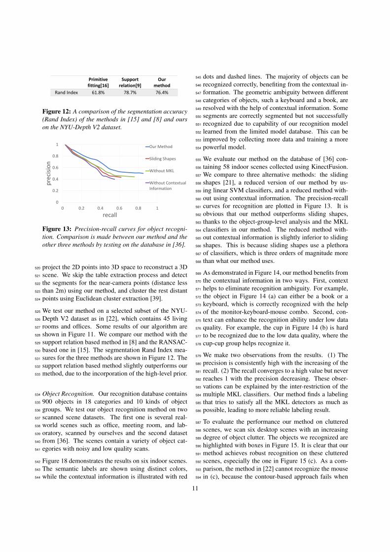
Primitive fitting[16]

Supportrelation[9]

Ourmethod

Rand Index 61.8% 78.7% 76.4%

Figure 12: A comparison of the segmentation accuracy(Rand Index) of the methods in [15] and [8] and ourson the NYU-Depth V2 dataset.

0

0.2

0.4

0.6

0.8

1

0 0.2 0.4 0.6 0.8 1

pre

cisi

on

recall

Our Method

Sliding Shapes

Without MKL

Without ContextualInformation

Figure 13: Precision-recall curves for object recogni-tion. Comparison is made between our method and theother three methods by testing on the database in [36].

project the 2D points into 3D space to reconstruct a 3D520

scene. We skip the table extraction process and detect521

the segments for the near-camera points (distance less522

than 2m) using our method, and cluster the rest distant523

points using Euclidean cluster extraction [39].524

We test our method on a selected subset of the NYU-525

Depth V2 dataset as in [22], which contains 45 living526

rooms and offices. Some results of our algorithm are527

shown in Figure 11. We compare our method with the528

support relation based method in [8] and the RANSAC-529

based one in [15]. The segmentation Rand Index mea-530

sures for the three methods are shown in Figure 12. The531

support relation based method slightly outperforms our532

method, due to the incorporation of the high-level prior.533

Object Recognition. Our recognition database contains534

900 objects in 18 categories and 10 kinds of object535

groups. We test our object recognition method on two536

scanned scene datasets. The first one is several real-537

world scenes such as office, meeting room, and lab-538

oratory, scanned by ourselves and the second dataset539

from [36]. The scenes contain a variety of object cat-540

egories with noisy and low quality scans.541

Figure 18 demonstrates the results on six indoor scenes.542

The semantic labels are shown using distinct colors,543

while the contextual information is illustrated with red544

dots and dashed lines. The majority of objects can be545

recognized correctly, benefiting from the contextual in-546

formation. The geometric ambiguity between different547

categories of objects, such a keyboard and a book, are548

resolved with the help of contextual information. Some549

segments are correctly segmented but not successfully550

recognized due to capability of our recognition model551

learned from the limited model database. This can be552

improved by collecting more data and training a more553

powerful model.554

We evaluate our method on the database of [36] con-555

taining 58 indoor scenes collected using KinectFusion.556

We compare to three alternative methods: the sliding557

shapes [21], a reduced version of our method by us-558

ing linear SVM classifiers, and a reduced method with-559

out using contextual information. The precision-recall560

curves for recognition are plotted in Figure 13. It is561

obvious that our method outperforms sliding shapes,562

thanks to the object-group-level analysis and the MKL563

classifiers in our method. The reduced method with-564

out contextual information is slightly inferior to sliding565

shapes. This is because sliding shapes use a plethora566

of classifiers, which is three orders of magnitude more567

than what our method uses.568

As demonstrated in Figure 14, our method benefits from569

the contextual information in two ways. First, context570

helps to eliminate recognition ambiguity. For example,571

the object in Figure 14 (a) can either be a book or a572

keyboard, which is correctly recognized with the help573

of the monitor-keyboard-mouse combo. Second, con-574

text can enhance the recognition ability under low data575

quality. For example, the cup in Figure 14 (b) is hard576

to be recognized due to the low data quality, where the577

cup-cup group helps recognize it.578

We make two observations from the results. (1) The579

precision is consistently high with the increasing of the580

recall. (2) The recall converges to a high value but never581

reaches 1 with the precision decreasing. These obser-582

vations can be explained by the inter-restriction of the583

multiple MKL classifiers. Our method finds a labeling584

that tries to satisfy all the MKL detectors as much as585

possible, leading to more reliable labeling result.586

To evaluate the performance our method on cluttered587

scenes, we scan six desktop scenes with an increasing588

degree of object clutter. The objects we recognized are589

highlighted with boxes in Figure 15. It is clear that our590

method achieves robust recognition on these cluttered591

scenes, especially the one in Figure 15 (c). As a com-592

parison, the method in [22] cannot recognize the mouse593

in (c), because the contour-based approach fails when594

11

(a) (b)

Figure 14: The contextual knowledge could benefit ob-ject recognition in two ways. (a): Resolving recognitionambiguity: The keyboard in blue box is recognized cor-rectly due to the contextual information of the monitor-keyboard-mouse combo. (b): Enhancing recognitionability: The cup in blue box is in low scan quality butcan be recognized based on the cup-cup combo.

(a)

(f)(e)

(d)(c)

(b)

Figure 15: Our recognition results on several sceneswith increasing degree of object from (a) to (f). Themonitors, keyboards and mouses are correctly recog-nized by our method and labeled with blue, orange andgreen boxes.

dealing with cluttered scenes due to the incorrect con-595

tour extraction. The contour of the red box area in (c) is596

shown on the top-right corner.597

(a) (b)

(c)

bottle

book

indeterminacy

Figure 16: A failure case of our method. Our methodcannot recognize most of the objects in a cluttered scene(c). This is due to the fact that the scene point cloud isonly a single-view scan (b).

Time Performance. For a scene with 100K points, the598

segment detection takes 20 seconds. The training proce-599

dure of our object recognition is determined by the num-600

ber of individual object and object group categories. In601

our case, it takes about 1 hour to train a classifier us-602

ing SimpleMKL averagely. The training process takes603

about 32 hours in total for the 18 objects and the 10 ob-604

ject groups. The testing time is determined by the num-605

ber of segments and the degree of object clutter. The606

testing time for the scenes in Figure 18 (a) to (f) are 7.8,607

19.1, 39.5, 20.3, 1.7 and 12.9 minutes, respectively.608

Limitations. Our method has the following limitations.609

First, our method does not provide a mechanism to deal610

with input data with severe missing parts. For example,611

if the input contains only a single-view scan, our method612

would not be able to produce meaningful segments for613

further analysis. A failure case of this is shown in Fig-614

ure 16. Second, our method can tolerate only moder-615

ate shape variation. It might fail when recognizing ob-616

jects with too special structure of segment graph, such617

as the case shown in Figure 17. Last, our method works618

the best for a scene containing a planar support. Al-619

though quite commonly seen in everyday indoor envi-620

ronments, the assumption does not generalize well for621

outdoor scenes.622

12

monitor

keyboard

mouse

cup

lamp

laptop

indeterminacy

globe

(c)

(e)

(f)

(a) (b)

(d)

cylinder

book

bottle

Figure 18: A gallery of scene understanding results by our method.

7. Discussion and future work623

To achieve object analysis from clustered subscenes, we624

have developed a unified framework for the discovery of625

both individual objects and object groups, both of which626

are based on the contextual information learned from a627

database of 3D scene models. Our method makes the628

contextual information applicable even without know-629

ing the object segmentation of the input scene. The lat-630

ter has so far been predominantly assumed by existing631

methods, e.g., [22].632

We see three venues for future work. First, our current633

work focuses on subscene analysis. It would be inter-634

esting to extend our method to deal with whole scene,635

leading to multi-scale scene analysis in a unified frame-636

work. Currently, the contextual information is based on637

spatial proximity. As another future work, we would638

like to expand our contextual features with multi-modal639

object interaction, such as dynamic motion, to address640

more complex mutual relations among objects. Finally,641

it is natural to utilize our framework in robot-operated642

autonomous scene scanning and understanding.643

Acknowledgements644

We thank all the reviewers for their comments and feed-645

back. We would also like to acknowledge our research646

grants: NSFC (61572507, 61202333, 61379103),647

13

(a) (b)

…

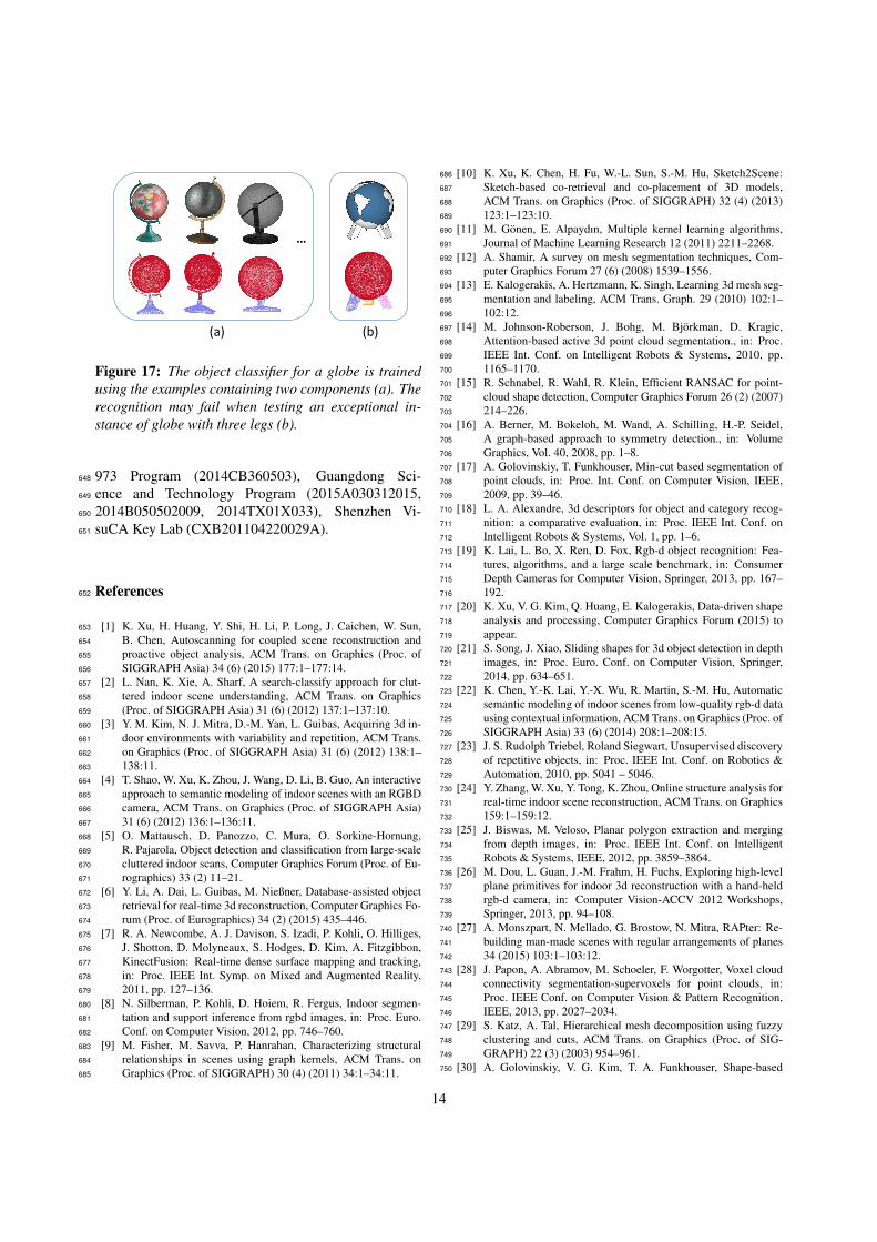
Figure 17: The object classifier for a globe is trainedusing the examples containing two components (a). Therecognition may fail when testing an exceptional in-stance of globe with three legs (b).

973 Program (2014CB360503), Guangdong Sci-648

ence and Technology Program (2015A030312015,649

2014B050502009, 2014TX01X033), Shenzhen Vi-650

suCA Key Lab (CXB201104220029A).651

References652

[1] K. Xu, H. Huang, Y. Shi, H. Li, P. Long, J. Caichen, W. Sun,653

B. Chen, Autoscanning for coupled scene reconstruction and654

proactive object analysis, ACM Trans. on Graphics (Proc. of655

SIGGRAPH Asia) 34 (6) (2015) 177:1–177:14.656

[2] L. Nan, K. Xie, A. Sharf, A search-classify approach for clut-657

tered indoor scene understanding, ACM Trans. on Graphics658

(Proc. of SIGGRAPH Asia) 31 (6) (2012) 137:1–137:10.659

[3] Y. M. Kim, N. J. Mitra, D.-M. Yan, L. Guibas, Acquiring 3d in-660

door environments with variability and repetition, ACM Trans.661

on Graphics (Proc. of SIGGRAPH Asia) 31 (6) (2012) 138:1–662

138:11.663

[4] T. Shao, W. Xu, K. Zhou, J. Wang, D. Li, B. Guo, An interactive664

approach to semantic modeling of indoor scenes with an RGBD665

camera, ACM Trans. on Graphics (Proc. of SIGGRAPH Asia)666

31 (6) (2012) 136:1–136:11.667

[5] O. Mattausch, D. Panozzo, C. Mura, O. Sorkine-Hornung,668

R. Pajarola, Object detection and classification from large-scale669

cluttered indoor scans, Computer Graphics Forum (Proc. of Eu-670

rographics) 33 (2) 11–21.671

[6] Y. Li, A. Dai, L. Guibas, M. Nießner, Database-assisted object672

retrieval for real-time 3d reconstruction, Computer Graphics Fo-673

rum (Proc. of Eurographics) 34 (2) (2015) 435–446.674

[7] R. A. Newcombe, A. J. Davison, S. Izadi, P. Kohli, O. Hilliges,675

J. Shotton, D. Molyneaux, S. Hodges, D. Kim, A. Fitzgibbon,676

KinectFusion: Real-time dense surface mapping and tracking,677

in: Proc. IEEE Int. Symp. on Mixed and Augmented Reality,678

2011, pp. 127–136.679

[8] N. Silberman, P. Kohli, D. Hoiem, R. Fergus, Indoor segmen-680

tation and support inference from rgbd images, in: Proc. Euro.681

Conf. on Computer Vision, 2012, pp. 746–760.682

[9] M. Fisher, M. Savva, P. Hanrahan, Characterizing structural683

relationships in scenes using graph kernels, ACM Trans. on684

Graphics (Proc. of SIGGRAPH) 30 (4) (2011) 34:1–34:11.685

[10] K. Xu, K. Chen, H. Fu, W.-L. Sun, S.-M. Hu, Sketch2Scene:686

Sketch-based co-retrieval and co-placement of 3D models,687

ACM Trans. on Graphics (Proc. of SIGGRAPH) 32 (4) (2013)688

123:1–123:10.689

[11] M. Gonen, E. Alpaydın, Multiple kernel learning algorithms,690

Journal of Machine Learning Research 12 (2011) 2211–2268.691

[12] A. Shamir, A survey on mesh segmentation techniques, Com-692

puter Graphics Forum 27 (6) (2008) 1539–1556.693

[13] E. Kalogerakis, A. Hertzmann, K. Singh, Learning 3d mesh seg-694

mentation and labeling, ACM Trans. Graph. 29 (2010) 102:1–695

102:12.696

[14] M. Johnson-Roberson, J. Bohg, M. Bjorkman, D. Kragic,697

Attention-based active 3d point cloud segmentation., in: Proc.698

IEEE Int. Conf. on Intelligent Robots & Systems, 2010, pp.699

1165–1170.700

[15] R. Schnabel, R. Wahl, R. Klein, Efficient RANSAC for point-701

cloud shape detection, Computer Graphics Forum 26 (2) (2007)702

214–226.703

[16] A. Berner, M. Bokeloh, M. Wand, A. Schilling, H.-P. Seidel,704

A graph-based approach to symmetry detection., in: Volume705

Graphics, Vol. 40, 2008, pp. 1–8.706

[17] A. Golovinskiy, T. Funkhouser, Min-cut based segmentation of707

point clouds, in: Proc. Int. Conf. on Computer Vision, IEEE,708

2009, pp. 39–46.709

[18] L. A. Alexandre, 3d descriptors for object and category recog-710

nition: a comparative evaluation, in: Proc. IEEE Int. Conf. on711

Intelligent Robots & Systems, Vol. 1, pp. 1–6.712

[19] K. Lai, L. Bo, X. Ren, D. Fox, Rgb-d object recognition: Fea-713

tures, algorithms, and a large scale benchmark, in: Consumer714

Depth Cameras for Computer Vision, Springer, 2013, pp. 167–715

192.716

[20] K. Xu, V. G. Kim, Q. Huang, E. Kalogerakis, Data-driven shape717

analysis and processing, Computer Graphics Forum (2015) to718

appear.719

[21] S. Song, J. Xiao, Sliding shapes for 3d object detection in depth720

images, in: Proc. Euro. Conf. on Computer Vision, Springer,721

2014, pp. 634–651.722

[22] K. Chen, Y.-K. Lai, Y.-X. Wu, R. Martin, S.-M. Hu, Automatic723

semantic modeling of indoor scenes from low-quality rgb-d data724

using contextual information, ACM Trans. on Graphics (Proc. of725

SIGGRAPH Asia) 33 (6) (2014) 208:1–208:15.726

[23] J. S. Rudolph Triebel, Roland Siegwart, Unsupervised discovery727

of repetitive objects, in: Proc. IEEE Int. Conf. on Robotics &728

Automation, 2010, pp. 5041 – 5046.729

[24] Y. Zhang, W. Xu, Y. Tong, K. Zhou, Online structure analysis for730

real-time indoor scene reconstruction, ACM Trans. on Graphics731

159:1–159:12.732

[25] J. Biswas, M. Veloso, Planar polygon extraction and merging733

from depth images, in: Proc. IEEE Int. Conf. on Intelligent734

Robots & Systems, IEEE, 2012, pp. 3859–3864.735

[26] M. Dou, L. Guan, J.-M. Frahm, H. Fuchs, Exploring high-level736

plane primitives for indoor 3d reconstruction with a hand-held737

rgb-d camera, in: Computer Vision-ACCV 2012 Workshops,738

Springer, 2013, pp. 94–108.739

[27] A. Monszpart, N. Mellado, G. Brostow, N. Mitra, RAPter: Re-740

building man-made scenes with regular arrangements of planes741

34 (2015) 103:1–103:12.742

[28] J. Papon, A. Abramov, M. Schoeler, F. Worgotter, Voxel cloud743

connectivity segmentation-supervoxels for point clouds, in:744

Proc. IEEE Conf. on Computer Vision & Pattern Recognition,745

IEEE, 2013, pp. 2027–2034.746

[29] S. Katz, A. Tal, Hierarchical mesh decomposition using fuzzy747

clustering and cuts, ACM Trans. on Graphics (Proc. of SIG-748

GRAPH) 22 (3) (2003) 954–961.749

[30] A. Golovinskiy, V. G. Kim, T. A. Funkhouser, Shape-based750

14

recognition of 3d point clouds in urban environments, in: Proc.751

Int. Conf. on Computer Vision, 2009, pp. 2154–2161.752

[31] Y. Cheng, Mean shift, mode seeking, and clustering, IEEE753

Trans. Pattern Analysis & Machine Intelligence 17 (8) (1995)754

790–799.755

[32] N. J. Mitra, M. Wand, H. Zhang, D. Cohen-Or, V. Kim, Q.-756

X. Huang, Structure-aware shape processing, in: ACM SIG-757

GRAPH 2014 Courses, 2014.758

[33] K. Xu, R. Ma, H. Zhang, C. Zhu, A. Shamir, D. Cohen-Or,759

H. Huang, Organizing heterogeneous scene collection through760

contextual focal points, ACM Trans. on Graphics (Proc. of SIG-761

GRAPH) 33 (4) (2014) 35:1–35:12.762

[34] C. Zhu, X. Liu, Q. Liu, Y. Ming, J. Yin, Distance based multiple763

kernel elm: A fast multiple kernel learning approach, Mathe-764

matical Problems in Engineering 2015.765

[35] M. Kazhdan, H. Hoppe, Screened poisson surface reconstruc-766

tion, ACM Trans. on Graphics 32 (3) (2013) 29:1–29:13.767

[36] A. Karpathy, S. Miller, L. Fei-Fei, Object discovery in 3d scenes768

via shape analysis, in: Proc. IEEE Int. Conf. on Robotics &769

Automation, IEEE, 2013, pp. 2088–2095.770

[37] A. Rakotomamonjy, F. Bach, S. Canu, Y. Grandvalet, Sim-771

pleMKL, Journal of Machine Learning Research 9 (2008) 2491–772

2521.773

[38] J. Chen, D. Bautembach, S. Izadi, Scalable real-time volumet-774

ric surface reconstruction, ACM Trans. on Graphics (Proc. of775

SIGGRAPH) 32 (4) (2013) 113:1–113:16.776

[39] D. Sparks, Euclidean cluster analysis, Applied Statistics (1973)777

126–130.778

15