POLITECNICO DI MILANOSchool of Industrial and Information Engineering

Master of Science in Automation and Control Engineering

Data-driven attitude control design formultirotor UAVs

Advisor: Prof. Marco LOVERACo-Advisor: Ing. Pietro PANIZZA

Ing. Davide INVERNIZZIIng. Mattia GIURATO

Thesis by:Thibaud Chupin Matr. 821382

Academic Year 2015–2016

Voici mon secret. Il est très simple: on ne voit bien qu’avec le cœur.L’essentiel est invisible pour les yeux.

– Le Renard, Dans Le Petit Prince, Antoine de Saint Exupéry

Here is my secret. It is very simple: It is only with the heart that one cansee rightly; what is essential is invisible to the eye.

– The Fox, In The Little Prince, Antoine de Saint Exupéry

Acknowledgements

Research is always a collaborative effort and it would be remiss of me if Idid not thank all those who helped.

I would like to like to express my deep gratitude to Professor Loverafor offering me the opportunity to work on a project this interesting. Hispatience and guidance were essential to the completion of this work.

I must also thank Professor Ferrigno and Professor De Momi for theirsupport during these last months. Without their encouragement I may neverhave graduated.

I would also like to thank Pietro Panizza, Davide Invernizzi and MattiaGiurato for their help. Without their understanding of control theory andquadrotors I doubt whether I would ever have been able to finish.

Finally I would like to thank my parents for always believing in me evenwhen I was ready to give up.

I

Abstract

Small multirotor unmanned aerial vehicles (UAV) are a ground-breakinginvention. They have made accessible to hobbyists and professionals aliketechnologies that, until recently, were prohibitively expensive. They are usedby farmers to survey their fields and evaluate their fertility, by videographerslooking to capture impressive images in remote and inaccessible areas or bypower companies to monitor the state of high voltage power lines for example.These are but a sample of the infinite applications of such vehicles. Thesevehicles are, simple , sturdy and affordable. The downside is the relativecomplexity of the control schemes required to pilot them. A complex attitudecontrol system is required to make the vehicle controllable.

The most complex part of a multirotor is the control software imple-menting the attitude and position control loops. In traditional controllersynthesis a prerequisite is the availability of an accurate model of the systemthe development of which is non-trivial. An alternative approach is offered byso-called data-driven methods. These methods identify a suitable controllerby solving a parameter identification problem and thus avoid the need todevelop a model.

The goal of this thesis is to use the latter methods to obtain an attitudecontroller with performance at least as good as what has been previouslyachieved with traditional methods. In detail, the reasoning behind the choiceof the specific controller tuning algorithm will be presented following whichthe methodology used to develop the controllers in practice will be exposed.Most importantly, the results obtained from both a simulation of the systemand experimental tests will be shown.

III

Contents

Acknowledgements I

Abstract III

Introduction 1

1 Quadrotors & Attitude Control 5

1.1 Design Considerations . . . . . . . . . . . . . . . . . . . . . . 6

1.2 Control of a Fixed Pitch Quadcopter . . . . . . . . . . . . . . 7

1.2.1 Elevation . . . . . . . . . . . . . . . . . . . . . . . . . 8

1.2.2 Roll . . . . . . . . . . . . . . . . . . . . . . . . . . . . 8

1.2.3 Pitch . . . . . . . . . . . . . . . . . . . . . . . . . . . . 9

1.2.4 Yaw . . . . . . . . . . . . . . . . . . . . . . . . . . . . 9

1.2.5 Longitudinal & Lateral translation . . . . . . . . . . . 9

1.3 The Attitude Control Loops . . . . . . . . . . . . . . . . . . . 10

1.3.1 The Pitch Control Loop . . . . . . . . . . . . . . . . . 10

1.3.2 The Roll Control Loop . . . . . . . . . . . . . . . . . . 12

1.3.3 The Yaw Control Loop . . . . . . . . . . . . . . . . . . 12

2 Data Driven Control Methods: State of the Art 15

2.1 The Classical Approach . . . . . . . . . . . . . . . . . . . . . 15

V

2.2 Model-Reference Controller Tuning . . . . . . . . . . . . . . . 16

2.2.1 Model-Based Control . . . . . . . . . . . . . . . . . . . 17

2.2.2 Data-Driven Control . . . . . . . . . . . . . . . . . . . 18

2.2.3 Comparison of the data-driven methods . . . . . . . . 22

2.3 VRFT In Detail . . . . . . . . . . . . . . . . . . . . . . . . . 23

2.3.1 A Rigorous Explanation . . . . . . . . . . . . . . . . . 24

2.3.2 The Method Step By Step . . . . . . . . . . . . . . . . 30

2.3.3 The Problem of Noisy Data . . . . . . . . . . . . . . . 30

2.3.4 Extension to Cascade Control . . . . . . . . . . . . . . 32

2.3.5 The Cascade VRFT Method Step By Step . . . . . . . 35

3 Simulation Results 37

3.1 Simulated Model . . . . . . . . . . . . . . . . . . . . . . . . . 37

3.1.1 Pitch Dynamics . . . . . . . . . . . . . . . . . . . . . . 37

3.1.2 Mixer Matrix . . . . . . . . . . . . . . . . . . . . . . . 38

3.1.3 Complete System . . . . . . . . . . . . . . . . . . . . . 40

3.2 Structure of the Reference Models . . . . . . . . . . . . . . . 41

3.2.1 Inner Reference Model . . . . . . . . . . . . . . . . . . 41

3.2.2 Outer Reference Model . . . . . . . . . . . . . . . . . 42

3.3 Controller Families . . . . . . . . . . . . . . . . . . . . . . . . 42

3.4 Simulation Results . . . . . . . . . . . . . . . . . . . . . . . . 43

4 Experimental Results 51

4.1 Quadcopter Hardware & Firmware . . . . . . . . . . . . . . . 51

4.1.1 Frame . . . . . . . . . . . . . . . . . . . . . . . . . . . 52

4.1.2 Motors, ESC & Propellers . . . . . . . . . . . . . . . . 52

4.1.3 Battery . . . . . . . . . . . . . . . . . . . . . . . . . . 52

4.1.4 Vibration Damping . . . . . . . . . . . . . . . . . . . . 52

4.1.5 Flight Control Unit & Firmware . . . . . . . . . . . . 54

4.1.6 Test Bed . . . . . . . . . . . . . . . . . . . . . . . . . 54

4.1.7 Additional Flight Hardware . . . . . . . . . . . . . . . 55

4.2 Tuning Experiment . . . . . . . . . . . . . . . . . . . . . . . . 55

4.3 Noise Considerations . . . . . . . . . . . . . . . . . . . . . . . 57

4.4 Reference Models . . . . . . . . . . . . . . . . . . . . . . . . . 58

4.4.1 Inner Reference Model . . . . . . . . . . . . . . . . . . 59

4.4.2 Outer Reference Model . . . . . . . . . . . . . . . . . 60

4.5 Results & Comparison . . . . . . . . . . . . . . . . . . . . . . 60

4.5.1 Set-Point Tracking . . . . . . . . . . . . . . . . . . . . 60

4.5.2 Disturbance Rejection . . . . . . . . . . . . . . . . . . 62

Bibliography 65

List of Figures

1.1 Illustartion of the Roll, Pitch & yaw Motions . . . . . . . . . 7

1.2 Rotation directions of the quadrotor propellers . . . . . . . . 8

1.3 The pitch control loop . . . . . . . . . . . . . . . . . . . . . . 10

1.4 The yaw control loop . . . . . . . . . . . . . . . . . . . . . . . 12

2.1 The standard form for structured H∞ synthesis . . . . . . . 16

2.2 Single degree of freedom controller . . . . . . . . . . . . . . . 17

2.3 Tuning scheme for correlation based tuning . . . . . . . . . . 20

2.4 Tuning scheme for VRFT . . . . . . . . . . . . . . . . . . . . 23

2.5 Control and reference model . . . . . . . . . . . . . . . . . . . 33

3.1 Simplified model of the quadcopter . . . . . . . . . . . . . . . 38

3.2 Measured & simulated open loop responses . . . . . . . . . . 39

3.3 Control Scheme used to simulate the pitch dynamics . . . . . 40

3.4 Simulated responses of the closed-loop transfer function andthe reference model . . . . . . . . . . . . . . . . . . . . . . . . 45

3.5 Simulated responses of the VRFT and H∞ tuned controllerswith an achievable reference model . . . . . . . . . . . . . . . 46

3.6 Bode plots for the inner closed-loop transfer function with anachievable reference model . . . . . . . . . . . . . . . . . . . . 47

3.7 Bode plots for the outer closed-loop transfer function with anachievable reference model . . . . . . . . . . . . . . . . . . . . 47

IX

3.8 Simulated responses of the VRFT and H∞ tuned controllerswith an unachievable reference model . . . . . . . . . . . . . . 49

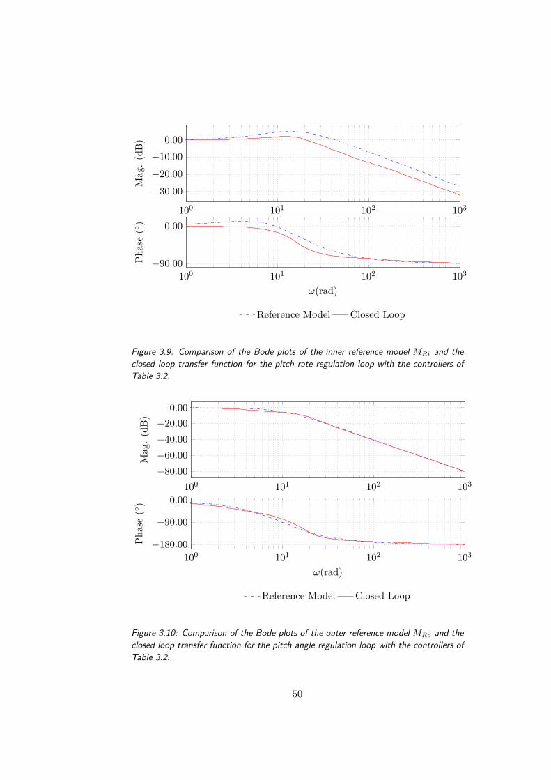
3.9 Bode plots for the inner closed-loop transfer function with anunachievable reference model . . . . . . . . . . . . . . . . . . 50

3.10 Bode plots for the outer closed-loop transfer function with anunachievable reference model . . . . . . . . . . . . . . . . . . 50

4.1 Quadrotor Components . . . . . . . . . . . . . . . . . . . . . 53

4.3 Pitch control scheme . . . . . . . . . . . . . . . . . . . . . . . 56

4.4 Tuning Experiment Inputs . . . . . . . . . . . . . . . . . . . . 57

4.5 Tuning Experiment Outputs . . . . . . . . . . . . . . . . . . . 58

4.6 VRFT set-point tracking . . . . . . . . . . . . . . . . . . . . . 61

4.7 H∞ set-point tracking . . . . . . . . . . . . . . . . . . . . . . 62

4.8 VRFT disturbance rejection . . . . . . . . . . . . . . . . . . . 63

4.9 H∞ disturbance rejection . . . . . . . . . . . . . . . . . . . . 63

List of Tables

3.1 VRFT results using an achievable reference model . . . . . . 44

3.2 VRFT results using an unachievable reference model . . . . . 48

4.1 VRFT & H∞ controller parameters . . . . . . . . . . . . . . . 60

4.2 Mean MSE of VRFT and H∞ experiments . . . . . . . . . . . 64

XI

Introduction

Throughout history the development of heavier than air vehicles can gen-erally be split between fixed wing aircraft (i.e.aeroplanes) and rotorcraft(i.e.helicopters). The former use engines aligned along the longitudinal axisof the vehicle to provide forward thrust, fixed wings for lift and a systemof control surfaces to generate the control torques and forces. The latterrely on a single large main rotor where the pitch angle of each blade canbe controlled which provides both lift and thrust as well as a smaller rotorto provide a counter-torque. The vehicle is then controlled by varying theindividual pitch of the rotor blades over the course of each rotation. Withfew exceptions, such as tilt-wing aircraft that have elements of both fixed androtary wing aircraft, this separation has remained accurate until recently.

Multirotor vehicles have emerged as a radically different approach toheavier than air flight. These are rotary wing aircraft that, instead ofdepending on a large main rotor for lift and control, employ many smallerrotors. Whereas a single large rotor requires a powerful (and thus expensive)motor to power, smaller rotors can be powered with smaller motors whosecumulative cost is less than the single large motor.

The downside is that the number of motors significantly complicates thecontrol scheme. Simple rotations and translations now require the combineduse of several motors which, in turn, requires a complex on-board flightcontrol unit (FCU). This FCU usually implements the different control loopsusing data from an on-board inertial measurement unit (IMU) that providesa continuously updated view of the aircraft’s orientation.

In turn the reduction in costs has created new opportunities: multi rotordrones are used for low-cost aerial surveying and mapping, airborne videoand photography or, more recently, delivery. This leads to a wide variety ofpayloads with different sizes and weights. This wide range of applications hasalso lead to a wide variety of vehicles: multirotors with three, four, six or even

1

eight rotors are quite common. Of these, the most common configurationis without a doubt the quadrotor: a machine with with four rotors. Thesehave been widely used to fly small payloads in the neighbourhood of 1kg,are relatively low cost and simple to control.

Thesis Description

The problem of attitude control in quadrotors is the focus of this thesis.With such a wide variety of vehicles sizes and applications a one-size-fits-allapproach cannot provide satisfactory results. The individual attitude con-trollers must be tuned manually to achieve acceptable levels of performance.This is usually done by first producing an accurate physical model of thequadcopter before applying classical control theory methods such as H∞tuning to synthesise a suitable controller. This procedure is long, complexbut most of all, is only performed once over the lifetime of the vehicle andcannot account for the degradation of the components as they age.

Data-driven methods represent an alternate approach to the controllersynthesis problem. Instead of requiring and accurate model of the systemthey rely entirely on the availability of a set of input-output data measuredin open loop conditions and directly produce the parameters of a controllerminimising a specified cost criterion.

These approaches are attractive firstly because they do not require anaccurate model of the system to be controlled but most of all because theycan be easily re-run to account for changes in the hardware of the system.One could for example periodically re-tune the controllers to account forthe aging of the components or even temperature variations. It may also bepossible to leverage this approach to automatically re-tune the controllers inflight to account for the specific size and shape of the payload.

This thesis represents a single early step on the way to such auto-tuningsystems. In it the applicability of a specific data-driven controller synthesistechnique: Virtual Reference Feedback Tuning to the pitch control loop andthe performance levels that can be achieved are explored. The results werecompared with a pre-existing H∞ -tuned controller.

2

Thesis Structure

The first chapter of this thesis aims to provide the reader with a more in-depthunderstanding of multirotor systems in general and, considering quadrotorsspecifically, the design considerations behind their structure. The secondhalf of the chapter concerns itself with an explanation of how a quadrotormoves and turns, which control inputs are required. This leads us to considerthe individual pitch, roll and yaw control loops and their structure.

The second chapter looks at controller tuning, comparing the classicalapproach with model-reference based methods. In talking about the lattermodel-based and data-driven approaches were considered before several differ-ent data-driven controller synthesis methods were detailed. After explainingwhy VRFT is the better choice for this problem an in depth explanation ofthis method is provided.

The third chapter looks at how the requirements on the system weretranslated for the VRFT method and how a known model can be used toguide the VRFT procedure. It shows how the simulated model was builtfrom the pre-existing knowledge of the machine and how this knowledgewas used to inform the structure of the reference models used to specifythe performance for the VRFT. Finally it shows how a set of input-outputdata was simulated to be used for the VRFT and the performance of thesimulated model.

The fourth and final chapter presents the specifics of the actual quadrotorthat was used for which the controller was tuned. It presents a brief overviewof the hardware components and the test-bed. It then shows how theinput-output data required for VRFT was collected and processed, how thereference models used were identified and finally it presents the results ofthe experiments testing campaign.

3

4

Chapter 1

Quadrotors & AttitudeControl

Quadrotors are multi-rotor aerial vehicles that exploit differential thrust fromtheir motors to move. Whilst quadrotors are the most common form of multi-rotor in use today they are not by any means the only one: configurationswith three (tricopters), six (hexacopters) and eight rotors (octocopters) havealso seen significant use.

Most multi-rotor designs strive to use relatively inexpensive commoditymotors to keep the system affordable. To that end, when trying to increasethe payload of the system it is often preferable to increase the number ofmotors instead of sourcing more powerful and more expensive motors capableof driving larger propellers. This naturally increases the effective payloadof the system as well as its redundancy. Whereas the loss of one motoron a tricopter or a quadcopter would have disastrous consequences on thecontrollability of the system, the loss of one motor on an octocopter mightbe relatively unnoticeable. The downside is that increasing the number ofmotors leads to a lower global efficiency compared to simply increasing theswept area of the rotors.

Quadcopters today have emerged as the standard architecture for lightweightsystems with payloads weighing in the neighbourhood of 1 kg. They provideacceptable levels of cost, redundancy, payload and performance and are usedwidely by hobbyists and professionals alike.

In Section 1.1 the general design considerations that must be taken intoaccount when designing a quadcopter will be briefly discussed following which

5

the control inputs necessary to achieve the various motions of the system willbe shown in Section 1.2. Finally, in Section 1.3 the various attitude controlloops will be shown.

1.1 Design Considerations

Unlike fixed wing aircraft that employ a complex system of control surfacesto generate control forces and moments, multicopters can only vary thethrust provided by each propeller. This can be achieved in a number of wayseach providing different trade-offs.

The most common way to vary the thrust of each propeller is to vary thespeed of each motor. This is the simplest way from both a mechanical andcontrol theory standpoint. By increasing or decreasing its speed, the amountof thrust produced by each propeller can be increased or decreased. Thissimplicity comes at a cost: the time constants of an electric motor spinningat several thousand rpm are comparatively high which limits the overallagility of the system.

A scheme that allows for faster reactions at the cost of complexity is totilt the arms onto which the motors are attached. In this configuration smallchanges in vertical thrust can be achieved with relatively small rotations ofthe arms. Whilst these can be actuated rather quickly, it is not possible toobtain large changes to the vertical thrust without also varying the speed ofthe propellers.

The fastest but most complex way of varying thrust is to control eachpropeller like the main rotor of a helicopter. A mechanical linkage allows thecontrol system to change the pitch angle of the blades of the propeller. Thisallows extremely fast changes in thrust but is significantly more complexmechanically. This configuration is generally reserved for larger quadcopterswhere the inertia of the propellers might make the previous methods tooslow.

A second important design choice is whether to adopt an X or a +structure. In the first configuration the motors are located on each side ofthe system, one at each tip of the X. In the latter configuration two motorsare situated along the longitudinal axis of the system: one in front of andone behind the centre. The other two motors are placed along the lateralaxis of the system: one right and one left of the centre.

6

The X configuration is often retained because it can provide more ro-tational acceleration and, if a camera is attached to the system it can bepointed forward without the landing gear being in its field of view.

The quad copter used for this work has an X configuration and fixedpitch rotors.

1.2 Control of a Fixed Pitch Quadcopter

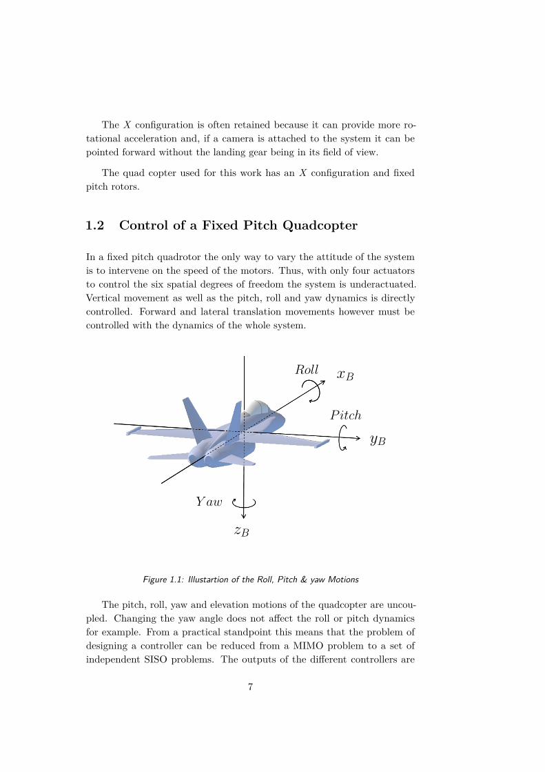
In a fixed pitch quadrotor the only way to vary the attitude of the systemis to intervene on the speed of the motors. Thus, with only four actuatorsto control the six spatial degrees of freedom the system is underactuated.Vertical movement as well as the pitch, roll and yaw dynamics is directlycontrolled. Forward and lateral translation movements however must becontrolled with the dynamics of the whole system.

Roll

P itch

Y aw

xB

yB

zB

Figure 1.1: Illustartion of the Roll, Pitch & yaw Motions

The pitch, roll, yaw and elevation motions of the quadcopter are uncou-pled. Changing the yaw angle does not affect the roll or pitch dynamicsfor example. From a practical standpoint this means that the problem ofdesigning a controller can be reduced from a MIMO problem to a set ofindependent SISO problems. The outputs of the different controllers are

7

simply summed to obtain a combined motion.

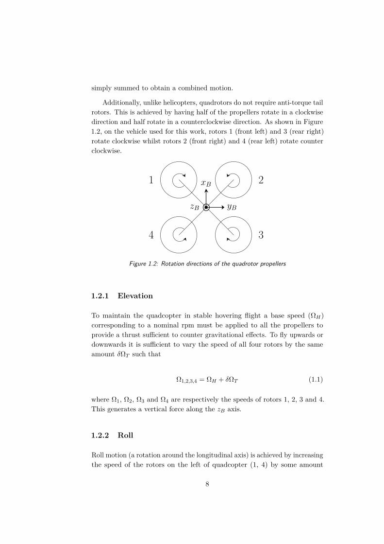
Additionally, unlike helicopters, quadrotors do not require anti-torque tailrotors. This is achieved by having half of the propellers rotate in a clockwisedirection and half rotate in a counterclockwise direction. As shown in Figure1.2, on the vehicle used for this work, rotors 1 (front left) and 3 (rear right)rotate clockwise whilst rotors 2 (front right) and 4 (rear left) rotate counterclockwise.

1 2

34

yB

xB

zB

Figure 1.2: Rotation directions of the quadrotor propellers

1.2.1 Elevation

To maintain the quadcopter in stable hovering flight a base speed (ΩH)corresponding to a nominal rpm must be applied to all the propellers toprovide a thrust sufficient to counter gravitational effects. To fly upwards ordownwards it is sufficient to vary the speed of all four rotors by the sameamount δΩT such that

Ω1,2,3,4 = ΩH + δΩT (1.1)

where Ω1, Ω2, Ω3 and Ω4 are respectively the speeds of rotors 1, 2, 3 and 4.This generates a vertical force along the zB axis.

1.2.2 Roll

Roll motion (a rotation around the longitudinal axis) is achieved by increasingthe speed of the rotors on the left of quadcopter (1, 4) by some amount

8

δΩR and decreasing the speed of the rotors on the right (2, 3) by the sameamount. This generates a torque around the xB axis of the quadcopter.

Ω1,4 = ΩH + δΩR

Ω2,3 = ΩH − δΩR.(1.2)

1.2.3 Pitch

Pitch motion (a rotation around the lateral axis) is obtained by increasingthe speed of the rotors on the front of the quadcopter (1, 2) by some amountδΩP and decreasing the speed of the rotors on the rear (3, 4) by the sameamount. This generates a torque around the yB axis of the quadcopter.

Ω1,2 = ΩH + δΩP

Ω3,4 = ΩH − δΩP .(1.3)

1.2.4 Yaw

Yaw motion (a rotation around the vertical axis) is achieved by increasing thespeed of the clockwise turning rotors by some amount δΩY and decreasingthe speed of the counterclockwise turning rotors by the same amount. Thisgenerates an imbalance of angular momenta around the zB axis which causesthe system to rotate around the vertical (zB) axis .

Ω1,3 = ΩH + δΩY

Ω2,4 = ΩH − δΩY .(1.4)

1.2.5 Longitudinal & Lateral translation

Longitudinal and lateral motions cannot be controlled directly with justfour control variables. Instead the dynamics of the entire system are usedto obtain these motions. Specifically, to move the quadcopter forward thesystem is tilted forward (pitched forward). To move backward the oppositemotion is applied. The same reasoning applies to lateral translations whereinstead of tilting around the pitch axis the system is rolled left and right.

9

1.3 The Attitude Control Loops

A closed loop control system is required in order to precisely control theorientation of the aircraft. In Section 1.2 we showed that the rotationaldegrees of freedom of the vehicle are uncoupled and that the attitude controlproblem can be viewed as a set of independent SISO problems.

When looking at a X -frame quadcopter, after removing any bodyworkand aerodynamic fairings, it can be quite difficult to differentiate the frontand the sides of the system. This symmetry is exploited when designing thecontrol system: the pitch and roll control loops can generally be consideredidentical. Only the yaw regulation loop differs.

Rather counter-intuitively the pitch and roll loops are stable. Theymust however be extremely reactive in order to compensate for externaldisturbances such as wind gusts.Thus, to maintain the vehicle in stable flightit is essential that these control loops be as fast as possible. The performanceof the yaw control loop by contrast is imposed not by physical imperatives butby the ability of the pilot. Whilst it would be possible to achieve extremelyhigh turn rates a human pilot must be able to control the vehicle and as suchthe bandwidth of this control loop is kept artificially low. This difference isapparent when comparing the structure of the pitch, roll and yaw controlloops. On the quadcopter used for this work the pitch and roll control areimplemented with a nested controller scheme whilst the yaw control loopuses a simpler single-loop architecture.

1.3.1 The Pitch Control Loop

The pitch control loop employs two nested loops to achieve the best possibleperformance. This is due to the fact that the pitch rate dynamics of thesystem, controlled by modifying the speed of the rotors, are considerablyfaster than the pitch angle dynamics.

PD(z) PID(z) QuadrotorPitch Dynamics

Mθo qo

q

θ

−−

Figure 1.3: The pitch control loop

10

The controllers implemented in the firmware of our quadcopter have afixed structure. The outer loop controller is a PD whereas the inner loopcontroller is a PID. These controllers are expressed in the ideal parallel form

PD(s) = Kpi + Kdis

Tf s + 1

PID(s) = Kpo + Kii

s+ Kdi

s

Tf s + 1

(1.5)

where Kpi , Kii and Kdiare respectively the proportional, integral and

derivative gains of the the PID controller, Kpo and Kdo are respectively theproportional and derivative gains of the the PD controller and Tf is the filtertime constant.

The control variable produced by the inner controller is the torque aroundthe pitch axis. The real input to the plant however is the difference in speedbetween the front rotors (numbers 1 & 2) and the rear rotors (numbers 3 & 4).The transformation from a torque to a speed difference is the responsibilityof the mixer matrix χ.

Consider the fact that each propeller generates a vertical thrust and, dueto the distance between the centre of the propeller and the centre of massof the vehicle, a torque. Consequently each propellers contributes to thevertical thrust T and the moments L, M and N around, respectively, thepitch, roll and yaw axes. It can be shown that the cumulative force generatedby the propellers is

FP rops =

00

KT

(Ω2

1 + Ω22 + Ω2

3 + Ω24) (1.6)

where Ωi is the rotational speed of the i-th motor and KT is a known constant.It can also be shown that cumulative moments L, M and N around the xB,yB and zB axes are

Mprops =

L

M

N

=

KT

b√2(Ω2

1 − Ω22 − Ω2

3 + Ω24)

KTb√2(Ω2

1 + Ω22 − Ω2

3 − Ω24)

KQ

(−Ω2

1 + Ω22 − Ω2

3 + Ω24) (1.7)

where KQ is another known constant. The forces and moments can berearranged in order to isolate on one side L, M , N and T and on the other

11

Ω21, Ω2

2, Ω23 and Ω2

4

T

L

M

N

=

KT KT KT KT

KTb√2 −KT

b√2 −KT

b√2 KT

b√2

KTb√2 KT

b√2 −KT

b√2 −KT

b√2

KQ KQ KQ KQ

Ω21

Ω22

Ω23

Ω24

= χ

Ω2

1Ω2

2Ω2

3Ω2

4

(1.8)

where χ is the mixer matrix which relates the required thrusts and momentsto around each axis to the rotational speed of each propeller.

1.3.2 The Roll Control Loop

The roll control loop as implemented on the quadcopter that was used for thiswork is identical to the pitch control described in Section 1.3.1. It differs onlyin the pairs of rotors it considers. The input to the plant is the difference inspeed between the right rotors (numbers 1 & 4) and the left rotors (number2 & 3).

1.3.3 The Yaw Control Loop

Due to its lower bandwidth requirements the Yaw control loop is the simplestof the attitude control loops.

PI(s) QuadrotorRoll Dynamics

qo eq N q

−

Figure 1.4: The yaw control loop

On this quadcopter the controller is implemented as a simple PI expressedin the ideal parallel form

PI(s) = Kp + Ki1s

(1.9)

12

which controls the angular rate of the system around the yaw axis. Unlike thepitch and roll loops the yaw control loop groups the motors by the directionof rotation of the propellers. The real control input is the difference in speedbetween the clockwise turning and the counterclockwise turning propellers.The transformation from an angular momentum to a speed difference isassured by the mixer matrix.

13

14

Chapter 2

Data Driven ControlMethods: State of the Art

Virtual Reference Feedback Tuning (VRFT) and its application to theproblem of attitude control is the focus of this thesis. VRFT is a data-drivencontroller synthesis technique, part of a more recent branch of control theorythat, instead of relying on the availability of a model, depend only on theexistence of a suitable set of input output data.

In Section 2.1 we will discuss the traditional approach to controllerdesign and specifically look at H∞ synthesis. In Section 2.2 we will exploremodel-reference methods, comparing model-based and data-driven approaches.Finally in Section 2.2.2 I will detail the virtual reference feedback tuningapproach.

2.1 The Classical Approach

In the traditional approach to controller synthesis the requirements on theclosed loop behaviour of the system are expressed as simple conditions on, forexample, the bandwidth of the system or its disturbance rejection properties.In addition some robustness requirements may be considered such as requiringa certain gain and phase margin.

One such method is H∞ synthesis. In this framework the requirementson the closed loop system are expressed as constraints on the H∞ normof its transfer function. This framework can extend the classical synthesis

15

techniques to multi-loop and MIMO control architectures. However, practicalconsiderations have slowed its adoption: whereas industrial controllers usuallyhave a decentralised architecture employing many simple controllers the H∞synthesis produces a monolithic high-order controller.

P (s)

K(s; θ)

u

w z

Figure 2.1: The standard form for structured H∞ synthesis

Structured H∞ synthesis is a solution to this problem. All the nontunable blocks of the system are combined into a single block P (s) and allthe tunable elements are merged into a single structured controller K(s; θ)parametrised in θ.

Solving the H∞ problem consists in identifying the parameter vector θ

that minimises

‖Tw→z (P (s), K(s; θ))‖∞ (2.1)

subject to the constraint that K(s; θ) stabilises P (s) where Tw→z(P (s), K(s; θ))is the closed loop transfer function from w to z on which the requirementsthe requirements have been imposed.

2.2 Model-Reference Controller Tuning

Model-reference approaches to controller tuning differ from traditional meth-ods in how the requirements for the controller are specified. Instead ofproviding explicit limits on overshoot, bandwidth or response time the re-quirements are provided in the form of a reference model for the closed loopbehaviour of the system.

The objective is to design a controller such that the difference betweenthe reference model and the actual closed-loop behaviour of the system is assmall as possible.

Consider the closed loop system shown in Figure 2.2 with the stablelinear SISO plant G(z), the controller C(z; ρ) parametrised in ρ and the

16

C(z; ρ) Gr e u y

−

ν

Figure 2.2: A generic closed loop system with a single degree of freedom controller anda disturbance on the output

stable strictly proper reference model MR(z). The objective of minimisingthe difference between the reference model and actual closed loop transferfunctions can be formulated as

Jmr(ρ) =∥∥∥∥MR(z) − C(z; ρ)G(z)

1 + C(z; ρ)G(z)

∥∥∥∥2

2. (2.2)

This is not the only possible control objective. Indeed, different methodsusually specify their own but they are usually similar in intent. In thisspecific case the ideal controller C0 is

C0(z) = M(z)G(z) (1 − M(z)) . (2.3)

We can identify two approaches to solving this problem:

• Model-Based approaches assume that a detailed and reliable modelof the plant is available in order to directly compute the ideal controller.

• Data-Driven approaches attempt to minimise the control objectiveJMR(ρ) by solving a parameter optimisation problem without firstestimating a model of the plant.

The following section will be dedicated to detailing both approaches andtheir limitations. We will also rapidly introduce several algorithms thatimplement data-driven approaches and explain their specific limitations inorder to justify our decision to use VRFT.

2.2.1 Model-Based Control

As previously noted, model-based approaches solve the model-referenceproblem by assuming that a plant model is available. This model may be

17

derived from an understanding of the underlying physics or obtained with anidentification procedure. This requires the collection of a sufficiently largeset of input-output data from the plant in open-loop conditions. The choiceof a high order model reduces the modelling error to such a level that it canbe considered negligible in later steps. The identified model is then used tocompute a full-order controller that minimises the control objective.

In many applications however the type of controller is pre-determined.Many industrial processes, for example, use pre-defined PID blocks and thecontrol procedure is limited to tuning the PID gains. If the tuning methodproduces only high-order controllers an additional model-order reduction pass.This step is generally problematic since any stability guarantees that wereformulated for the full-order controller may not transfer to the reduced-ordercontroller. Furthermore whilst the optimality of the full-order controller canbe guaranteed that is not the case for the reduced-controller. It may not evenbe the best controller in its class. For this reason, structured model-basedcontrol techniques have been developed using an approach similar to that ofstructured H∞ control.

2.2.2 Data-Driven Control

Data-driven controller tuning methods skip the modelling phase entirely andinstead reformulate the controller identification procedure as a parameteroptimisation problem in which the optimisation is carried out directly onthe controller parameters.

The principal advantage of data-driven methods compared to their model-based brethren is their ability to tune low-order controllers directly whereasmodel-based methods may produce n without having to first pass through amodel order reduction stage. This ensures that any stability or optimalityguarantees provided by these methods will not be lost. Furthermore, theachieved performance of the controllers is not linked to the techniques usedto model the plant or the order of the identified model.

In practice there are many ways to achieve this objective. In this sectionwe will detail several methods. In particular we will explain the functioningof Iterative FeedbackTuning (IFT), Correlation Based Tuning (CBT) andVirtual Reference Feedback Tuning (VRFT).

18

Iterative Feedback Tuning

IFT, originally described in [6], is an iterative method that uses a gradient-descent algorithm to compute a local minimum of the cost function. Thekey observation of IFT is that the chosen cost criterion can be estimated byusing carefully designed experiments on the plant.

Consider a generic closed loop system with a single degree of freedomcontroller as in Figure 2.2. Given a reference model MR(z) the desired outputof the plant in response to a reference input r is

yd = MR(z)r (2.4)

and consequently, the error between the achieved and desired responses is

y(ρ) = y(ρ) − yd (2.5)

where ρ is the parameter vector and the (ρ)-argument indicates that theterms were collected whilst the controller C(z; ρ) was in place. The controlobjective that IFT seeks to minimise is the following:

J(ρ) = 12N

E

[N∑

t=1[Ly(z)y(ρ)]2 + λ

N∑t=1

[Lu(z)u(ρ)]2]

(2.6)

where N is the number of points in the input-output dataset, Ly(z) and Lu(z)are frequency weighting terms and u(ρ) is the control variable measured withthe controller C(z; ρ) in place.

This criterion considers the L2-norm of the frequency weighted errorbetween the achieved and desired responses and penalises the frequencyweighted control action. An algebraic solution to this problem would requireknowledge of the partial derivatives ∂y

∂ρ(ρ) and ∂u∂ρ (ρ) which are unknown.

IFT elegantly repurposes the plant itself to solve the problem. Indeed,through careful choice of the input signals and simple computations thederivatives can be estimated as described in [6].

The estimate of the gradient can be updated at each iteration using thesesimple experiments in order to asymptotically approach the local optimumof the control objective. At each iteration these experiments are re-run andthe gradient is estimated.

19

Therein lies the main limitation of IFT and gradient-descent basedmethods in general: it can only guarantee a local optimum. Thus, the qualityof the achieved controller depends in large part on the choice of the startingguess for the parameters.

A very attractive property of the method is that it is even applicable tonon-linear systems. In this case the system should simply be linearised atevery iteration.

Correlation Based Tuning

CBT [8] is a one-shot method to obtain a controller that minimises thecontrol objective whilst only requiring that the input signal provided to theplant be persistently exciting. It re-frames the model-reference problem as adecorrelation problem using a single set of input-output data.

G 1 − MR C

MR

r +v+ y − ε

+

open-loop experiment

Figure 2.3: Tuning scheme for correlation based tuning

Consider the scheme in figure 2.3. If the model matching problem isperfectly solved then

MR = C0G

1 + C0G⇒ 1 − MR = 1

1 + C0G(2.7)

and consequently

MR = G(1 − MR)C0 (2.8)

as in the block diagram. Thus, the error ε(t; θ) can be computed as

ε(t; θ) = MRr − C(θ)(1 − MR)y= MRr − C(θ)(1 − MR)r − C(θ)(1 − MR)v.

(2.9)

20

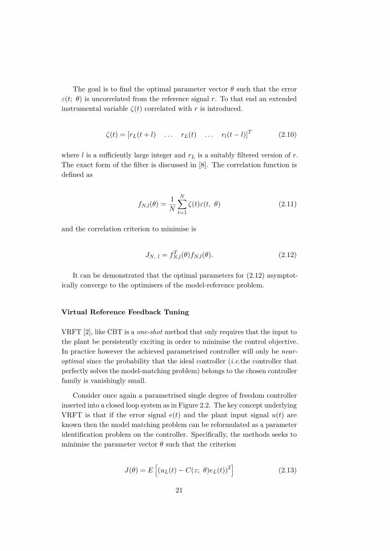
The goal is to find the optimal parameter vector θ such that the errorε(t; θ) is uncorrelated from the reference signal r. To that end an extendedinstrumental variable ζ(t) correlated with r is introduced.

ζ(t) = [rL(t + l) . . . rL(t) . . . rl(t − l)]T (2.10)

where l is a sufficiently large integer and rL is a suitably filtered version of r.The exact form of the filter is discussed in [8]. The correlation function isdefined as

fN,l(θ) = 1N

N∑t=1

ζ(t)ε(t, θ) (2.11)

and the correlation criterion to minimise is

JN, l = fTN,l(θ)fN,l(θ). (2.12)

It can be demonstrated that the optimal parameters for (2.12) asymptot-ically converge to the optimisers of the model-reference problem.

Virtual Reference Feedback Tuning

VRFT [2], like CBT is a one-shot method that only requires that the input tothe plant be persistently exciting in order to minimise the control objective.In practice however the achieved parametrised controller will only be near-optimal since the probability that the ideal controller (i.e.the controller thatperfectly solves the model-matching problem) belongs to the chosen controllerfamily is vanishingly small.

Consider once again a parametrised single degree of freedom controllerinserted into a closed loop system as in Figure 2.2. The key concept underlyingVRFT is that if the error signal e(t) and the plant input signal u(t) areknown then the model matching problem can be reformulated as a parameteridentification problem on the controller. Specifically, the methods seeks tominimise the parameter vector θ such that the criterion

J(θ) = E[(uL(t) − C(z; θ)eL(t))2

](2.13)

21

where L is an appropriate pre-filter for the data is minimised. Convenientlythis criterion is convex and can be expressed entirely in terms of the input-output data collected from the plant. Accordingly, the optimal parametervector is

θN =[∑

t

ϕL(t)ϕL(t)T

]−1∑t

ϕL(t)u(t). (2.14)

In the case of noisy measurements the method can be extended withthe use of a second input-output dataset using the same input signal andinstrumental variable based approach. This however may not always bepossible. Alternatively the noise can be estimated with an appropriate ARXmodel however identifying the correct order for the model is non-trivial andan incorrect choice will lead to unsatisfactory performance.

2.2.3 Comparison of the data-driven methods

The three data-driven methods presented previously all have different limita-tions and require different trade-offs.

IFT, being an iterative method, is comparatively slow and requires severalexperiments on the plant at each iteration. Moreover it can only guaranteethat the result is close to the local minimum of the cost function.

CBT is an extremely efficient method. It only requires one set of input-output data and some relatively simple calculations to to tune a globallyoptimal controller within the bounds of the chosen controller family.

VRFT is also very efficient computationally and data-wise. Furthermore,it has been extended in [4] to tune nested control loops of arbitrary depthswith a one shot procedure. The principal drawback of VRFT is the issue ofnoise. None of the proposed solutions are ideal.

Whilst an iterative procedure like IFT would be technically acceptable,the turnaround time due to many required experiments disqualified themethod from our consideration. In comparison CBT and VRFT both offerextremely fast turnaround times since many controllers can be tuned from thesame set of input-output data by simply changing the reference model. Thisallowed us to interactively explore the performance limitations of the system.These fast turnaround times also make it easy to re-tune the controllers tocompensate for payload changes or the degradation of the actuators due to

22

fatigue and temperature variations.

The final choice of VRFT was due to two predominant considerations:

• VRFT has already been successfully applied to the cascade controlproblem and a MATLAB toolbox implementing the method is available[3].

• significant pre-existing work exists documenting the application ofVRFT to quad-rotors (e.g., [7]).

Having detailed the reasons for the choice of VRFT to develop thecontrollers the method will now be presented in more detail.

2.3 VRFT In Detail

In VRFT the aim is to identify the parameters of a controller such that thecomplementary sensitivity of the system aligns with a user-specified referencemodel describing the desired behaviour of the closed loop system. This isachieved without requiring any knowledge of the structure of the system andusing only open-loop measurements.

The method is direct, it does not require a prior identification of theplant, and searches for a global optimum of the design criterion. Additionally,if the controller complexity is restricted the produced controller is a goodapproximation of the restricted complexity global optimal controller.

C(z; θ) P (z)

MR(z)

rve u y

−

y

Figure 2.4: Tuning scheme for VRFT

The method transforms the control problem into an identification problemthat minimises the L2-norm of the mismatch between the reference modeland the actual closed loop system.

If both the input and the output of the controller are known then it ispossible to find an optimal parameter vector that achieves this goal.

23

The key observation of this approach lies in the fact that this is possiblewhen the input signal of the reference model is chosen with care. If the inputwe provide to the reference model is such that its output is equal to themeasured output of the plant we can easily calculate the tracking error ofthe closed loop system.

2.3.1 A Rigorous Explanation

We assume that the plant under consideration is a linear SISO dynamicalsystem described by an unknown, rational transfer function P (z).

We also assume that a set of open-loop input-output data has beencollected during an experiment on the plant. The only requirement for thisexperiment is that it must excite the system over the entirety of the frequencyrange of interest. This experiment provides us two vectors of data-points

u = u0, u1, u2, . . . , uny = y1, y2, y3, . . . , yn .

We must also determine a reference model that describes the desiredclosed-loop behaviour of the system. Great care should be taken here tochoose a model that is physically achievable given the physical constraints ofthe system. If the reference model is unachievable the controller will be ofvery limited use. Let this reference model be MR(z).

Finally, we must decide on a family of controllers to tune. We restrictour attention to the class of controllers that can be expressed as a linearcombination of linear, discrete time, transfer functions. This controller familytakes the form

C(z; θ) = βT (z)θ (2.15)

where βT (z), the vector of linear transfer functions is

βT (z) = [β1(z), β2(z) . . . βn(z)]T

and θ, the parameter vector is

24

θ = [θ1, θ2 . . . θn]T .

The control objective is the minimisation of the following performancecriterion:

JMR(θ) =∥∥∥∥(MR(z) − P (z)C(z; θ)

1 + P (z)C(z; θ)

)W (z)

∥∥∥∥2

2

= ‖(T (z) − MR(z)) W (z)‖22

(2.16)

where T (z) is the complementary sensitivity function of the closed-loopsystem and W (z) is a user-specified weighting function.

The control objective penalises the difference between the closed-looptransfer function and the reference model scaled by an appropriate weightingfunction. This allows us to emphasize or de-emphasize performance in certainfrequency ranges.

The presence of the parameter vector in both the numerator and thedenominator of this function makes the minimisation problem non-convexwith respect to θ which significantly increases its difficulty.

In order to make the problem tractable an equivalent, convex optimisationcriterion must be identified. Consider now the following cost function:

JNV R(θ) = 1

N

N∑t=1

(uL(t) − C(z; θ) eL(t))2 (2.17)

where uL(t) and eL(t) are respectively the plant input and the tracking errormultiplied by a suitable pre-filter. Its form will be discussed later. Let thisfilter be L(z) and defined filtered versions of the signals u(t) and e(t) as

eL(t) = L(z)e(t)uL(t) = L(z)u(t).

(2.18)

Through simple transformations it is possible to rewrite the criterion as

25

JNV R(θ) = 1

N

N∑t=1

(uL(t) − βT (z)θeL(t)

)2

= 1N

N∑t=1

(uL(t) − ϕT

L(t)θ)2

, ϕL = βT (z)eL(t).(2.19)

Since this criterion is quadratic in θ the optimal parameter vector θ isan explicit function of the data

θN =[∑

t

ϕL(t)ϕL(t)T

]−1∑t

ϕL(t)u(t). (2.20)

We will now show that it is possible, through an appropriate choice ofthe pre-filter, to make the two cost functions (equations (2.16) and (2.17))equivalent.

Let JV R(θ) be the asymptotic counterpart of JNV R(θ). If u(t) and y(t)

can be considered realisations of stationary stochastic processes then as theamount of data grows (i.e., N → ∞) the minimum θN of JN

V R(θ) convergesto the minimum of JV R(θ), θ.

limN→∞

JNV R(θN ) = JV R(θ).

As such, the asymptotic criterion is

JV R(θ) = E[(uL(t) − C(z; θ)eL(t))2

]= E

[(L(z) (u(t) − C(z; θ)e(t)))2

].

(2.21)

The dependency on e(t) should be removed in order to make the criteriondepend only on the measured data. To that end we introduce rv(t), thereference signal that would feed the closed loop system when the closed looptransfer function is MR(z)

y(t) = MR(z)rv(t) (2.22)

from which we can deduce

26

rv(t) = 1MR(z)y(t)

= 1MR(z)P (z)u(t).

(2.23)

The signal rv(t) is not a physical signal, it was not used in the physicalexperiments to generate y(t) rather, y(t) was used to synthesise this signal.It is a tool used in the identification of the optimal controller. It is the virtualreference signal, the namesake of the method.

The tracking error of the closed loop system is

e(t) = rv(t) − y(t)= rv(t) − Mr(z)rv(t)= (1 − MR(z))rv(t)

(2.24)

and, by substituting the expression of rv(t) provided by equation (2.23) intothe tracking error (equation (2.24)) we obtain

e(t) = 1 − MR(z)MR(z) P (z)u(t) (2.25)

By substituting this new expression for e(t) into the cost function JV R

(equation 2.21) we can rewrite the cost function as

JV R(θ) = E

[(uL − C(θ)1 − MR

MRPuL

)2]

= E

[(L

(1 − C(θ)1 − MR

MRP

)u

)2]

.

(2.26)

Under our current hypothesis, the reference model MR(z) is equal to theclosed loop transfer function of the system

MR(z) = P (z)C0(z)1 + P (z)C0(z) (2.27)

where C0(z) is the ideal controller i.e., the controller that perfectly solvesthe model matching problem. Note that in general C0(z) might not belongto the family of parametrised controllers C(z; θ), be a proper rationaltransfer function or stabilise the closed loop system.

27

Additionally, observe that

1 − MR(z) = 1 + P (z)C0 − P (z)C0(z)1 + P (z)C0(z)

= 11 + P (z)C0(z)

(2.28)

from which

1 − C(z; θ)1 − MR(z)MR(z) P (z) = 1

MR(z) [MR(z) − P (z)C(z; θ) (1 − MR(z))]

= 1MR(z)

(P (z)C0(z)

1 + P (z)C0(z) − P (z)C(z; θ)1 + P (z)C0(z)

)= 1

MR(z)

(P (z) C0(z) − C(θ)

1 + P (z)C0(z)

).

(2.29)

If we substitute the previous result into the expression of the controlobjective derived in equation (2.26) we can rewrite it in a more convenientform

JV R(z; θ) = E

[(P (z)C0(z) − C(z; θ)

1 + P (z)C0(z)L(z)

MR(z)u

)2]. (2.30)

An alternative frequency domain representation of this criterion is

JV R(θ) = 12π

∫ π

−π

∣∣∣∣∣P (ejω)C0(ejω) − C(ejω; θ)1 + P (ejω)C0(ejω)

L(ejω)MR(ejω)

∣∣∣∣∣2

Φu(ω) dω

= 12π

∫ π

−π

∣∣∣∣∣(

PC0(ejω)1 + P (ejω)C0(ejω) − P (ejω)C(ejω; θ)

1 + P (ejω)C0(ejω)

)L(ejω)

MR(ejω)

∣∣∣∣∣2

Φu(ω) dω

(2.31)

where Φu(ω) is the power spectral density of the plant input u(t).

Observe that if C0(z) ∈ C(z; θ) and JV R(θ) has a unique minimumthen minimising JV R(θ) gives C0(z) for any choice of the filter L(z). Generallyhowever this is not the case and C0(z) 6∈ C(z; θ).

The expression of the initial control objective JMR(z) as given in equation(2.16) can be re-written in the following form:

28

JMR(θ) = 12π

∫ π

−π

∣∣∣∣∣MR(ejω) − P (ejω)C(ejω; θ)1 + P (ejω)C(ejω; θ)

∣∣∣∣∣2 ∣∣∣W (ejω)

∣∣∣2 dω

= 12π

∫ π

−π

∣∣∣∣∣ P (ejω)C0(ejω)1 + P (ejω)C0(ejω) − P (ejω)C(ejω; θ)

1 + P (ejω)C(ejω; θ)

∣∣∣∣∣2 ∣∣∣W (ejω)

∣∣∣2 dω.

(2.32)

There is a striking similarity between JMR and the new form of JV R. If thefilter were such that

∣∣∣L(ejω)∣∣∣2 =

∣∣∣∣∣ MR(ejω)W (ejω)1 + P (ejω)C(ejω; θ)

∣∣∣∣∣2 1

Φu(ω) , ∀ω ∈ [−π, π] (2.33)

then we would have JV R(θ) = JMR(θ) and, as a consequence, minimisingJV R would be equivalent to minimising JMR. Unfortunately, this choice ofL(z) is not practical since P (z) is not known. VRFT solves this problem byusing the following pre-filter on the measured data

∣∣∣L(ejω)∣∣∣2 =

∣∣∣(1 − MR(ejω))

MR(ejω)W (ejω)∣∣∣2 1

Φu(ω) , ∀ω ∈ [−π, π]

(2.34)

With the exception of the power spectral density of the input signal Φu,all the quantities on the right hand side of this filter are known. Φu canbe considered known only when the input signal has been selected by thecontrol system designer. In the general case it must be estimated.

Whilst on first approach the two different expressions of L(ejω) in equa-tions (2.33) and (2.34) may have little in common, their parentage becomesobvious if, exploiting (2.28), we re-write the latter as

∣∣∣L(ejω)∣∣∣2 =

∣∣∣∣∣ MR(ejω)W (ejω)1 + P (ejω)C0(ejω)

∣∣∣∣∣2 1

Φu(ω) , ∀ω ∈ [−π, π] (2.35)

which makes it clear that this choice of L(ejω) is equivalent to substituting|1 + PC(θ)|2 for |1 + PC0|2. This is a sensible choice if, as required, C(θ) isa good approximation of C0.

29

In conclusion, by a judicious choice of the pre-filter L(z) it is possible torender the optimisation problem convex and purely quadratic in θ. This, inturn, makes the optimisation problem trivial to solve.

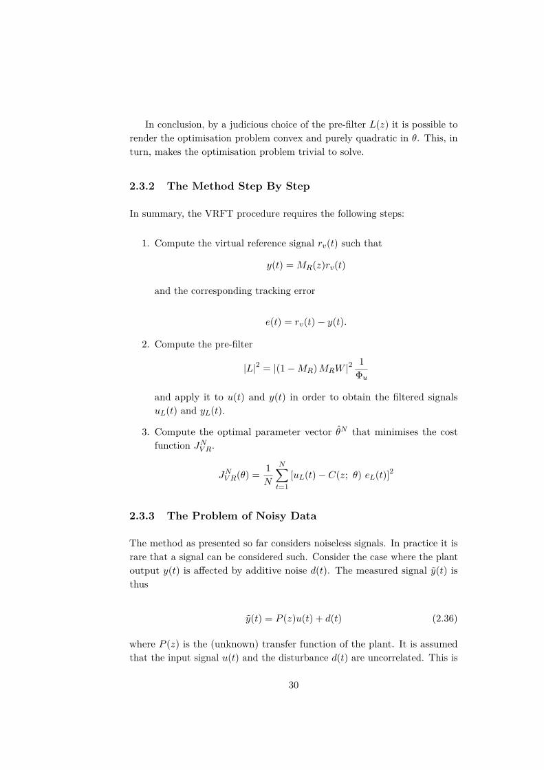
2.3.2 The Method Step By Step

In summary, the VRFT procedure requires the following steps:

1. Compute the virtual reference signal rv(t) such that

y(t) = MR(z)rv(t)

and the corresponding tracking error

e(t) = rv(t) − y(t).

2. Compute the pre-filter

|L|2 = |(1 − MR) MRW |2 1Φu

and apply it to u(t) and y(t) in order to obtain the filtered signalsuL(t) and yL(t).

3. Compute the optimal parameter vector θN that minimises the costfunction JN

V R.

JNV R(θ) = 1

N

N∑t=1

[uL(t) − C(z; θ) eL(t)]2

2.3.3 The Problem of Noisy Data

The method as presented so far considers noiseless signals. In practice it israre that a signal can be considered such. Consider the case where the plantoutput y(t) is affected by additive noise d(t). The measured signal y(t) isthus

y(t) = P (z)u(t) + d(t) (2.36)

where P (z) is the (unknown) transfer function of the plant. It is assumedthat the input signal u(t) and the disturbance d(t) are uncorrelated. This is

30

generally the case in open loop configurations. If we were to apply the VRFTmethod to this noisy data the performance would be significantly affected bynoise. This is clearly evidenced by the frequency domain of the asymptoticcriterion JV R(θ). Considering the effect of the additive noise it becomes

JV R(θ) = 12π

∫ π

−π

∣∣∣∣∣P (ejω)C0(ejω) − C(ejω; θ)1 + P (ejω)C0(ejω)

L(ejω)MR(ejω)

∣∣∣∣∣2

Φu(ω) dω

+ 12π

∫ π

−π

∣∣∣∣∣ C(ejω; θ)P (ejω)C0(ejω)

∣∣∣∣∣2

Φd(ω)dω︸ ︷︷ ︸Bias due to disturbance

(2.37)

where Φd(ω) is the power spectral density of the disturbance. The disturbancecreates a bias in the criterion that needs to be overcome.

This is achieved with an instrumental variable method. We introducethe quantity

ϕL(t) = β(z)L(z)(M(z)−1 − 1

)y(t) (2.38)

as a replacement for ϕL(t) introduced in equation (2.19). We also introducethe instrumental variable ζ(t) and compute the optimal parameter vector as

θIVN =

[N∑

t=1ζ(t)ϕL(t)T

]−1 [ N∑t=1

ζ(t)uL(t)]

(2.39)

Two different choices for the instrumental variable have been proposedin the literature.

Instrumental Variable From Repeated Experiments

Instead of performing a single experiment on the plant, two experimentsmust be carried out with the same input signal. This yields three vectors ofdata points

u = u0, u1, u2, . . . , uny = y1, y2, y3, . . . , yny′ =

y′

1, y′2, y′

3, . . . , y′n

31

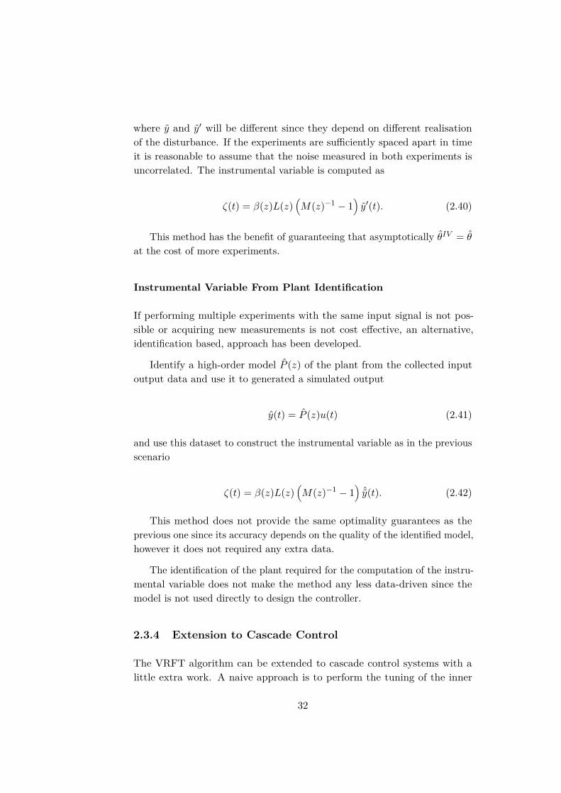
where y and y′ will be different since they depend on different realisationof the disturbance. If the experiments are sufficiently spaced apart in timeit is reasonable to assume that the noise measured in both experiments isuncorrelated. The instrumental variable is computed as

ζ(t) = β(z)L(z)(M(z)−1 − 1

)y′(t). (2.40)

This method has the benefit of guaranteeing that asymptotically θIV = θ

at the cost of more experiments.

Instrumental Variable From Plant Identification

If performing multiple experiments with the same input signal is not pos-sible or acquiring new measurements is not cost effective, an alternative,identification based, approach has been developed.

Identify a high-order model P (z) of the plant from the collected inputoutput data and use it to generated a simulated output

y(t) = P (z)u(t) (2.41)

and use this dataset to construct the instrumental variable as in the previousscenario

ζ(t) = β(z)L(z)(M(z)−1 − 1

)ˆy(t). (2.42)

This method does not provide the same optimality guarantees as theprevious one since its accuracy depends on the quality of the identified model,however it does not required any extra data.

The identification of the plant required for the computation of the instru-mental variable does not make the method any less data-driven since themodel is not used directly to design the controller.

2.3.4 Extension to Cascade Control

The VRFT algorithm can be extended to cascade control systems with alittle extra work. A naive approach is to perform the tuning of the inner

32

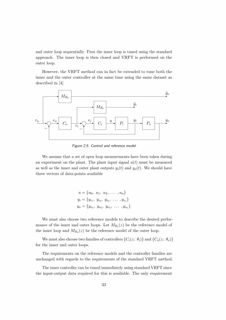
and outer loop sequentially. First the inner loop is tuned using the standardapproach. The inner loop is then closed and VRFT is performed on theouter loop.

However, the VRFT method can in fact be extended to tune both theinner and the outer controller at the same time using the same dataset asdescribed in [4].

Co Ci Pi Po

MRi

MRo

ro eo ei u yi yo

−− ri

yi

yo

Figure 2.5: Control and reference model

We assume that a set of open loop measurements have been taken duringan experiment on the plant. The plant input signal u(t) must be measuredas well as the inner and outer plant outputs yi(t) and yo(t). We should havethree vectors of data-points available

u = u0, u1, u2, . . . , unyi = yi1 , yi2 , yi3 , . . . , yinyo = yo1 , yo2 , yo3 , . . . , yon

We must also choose two reference models to describe the desired perfor-mance of the inner and outer loops. Let MRi(z) be the reference model ofthe inner loop and MRo(z) be the reference model of the outer loop.

We must also choose two families of controllers Ci(z; θi) and Co(z; θo)for the inner and outer loops.

The requirements on the reference models and the controller families areunchanged with regards to the requirements of the standard VRFT method.

The inner controller can be tuned immediately using standard VRFT sincethe input-output data required for this is available. The only requirement

33

imposed on the inner loop is that it be as close as possible to the referencemodel.

The outer loop is slightly more complex. In this case, to apply the VRFTalgorithm we must compute a new plant model that encompasses the entiretyof the inner loop and the outer plant as well as a signal analogous to theinner plant input u(t).

Calculating a new, extended, plant model is rather simple

G(z) = Ci(z)Pi(z)1 + Ci(z)Pi(z)Po(z)

Considering this enlarged plant, the input is simply ri(t), the referencesignal of the inner loop. In contrast with the inner loop however thissignal takes on a physical meaning, it is no longer a virtual reference signal.Additionally, since the original dataset was acquired in open-loop conditionsit is not part of our original dataset. Fortunately it can be computed quitesimply as

ri(t) = ei(t) + yi(t)

where the output yi(t) is part of our initial dataset and is known. The innertracking error ei(t) is entirely fictitious but since it derives directly fromthe design of the inner plant it is rather simple to compute. If the innercontroller Ci(z) is invertible then

ei(t) = C(z; θi)−1u(t).

This calculation only yields useful results if the inner controller isminimum-phase. If that is not the case it will have zeros located out-side of the limit cycle. When the controller is inverted these will becomeunstable poles. In turn they will cause the tracking error to diverge, makingthe signal quite useless for our purposes.

Unfortunately, VRFT provides no guarantees that the controllers it pro-duces will be minimum phase but in practice non-minimum phase controllersonly appear when the reference model is unachievable. Reducing the require-ments on the reference model is usually sufficient to obtain a suitable innercontroller.

34

Thus, the reference input for the outer loop is

ri(t) = C(z; θi)−1u(t) + yi(t).

Once the extended plant input ri(t) is known the outer controller can beeasily found with the classic VRFT synthesis using as input-output data theset of data-points ri(t), yo(t).

2.3.5 The Cascade VRFT Method Step By Step

To summarise, in order to tune both the inner and outer controllers of acascade control system using a single set of data the procedure is:

1. Compute the inner virtual reference riv(t) such that

yi(t) = Mi(z)riv(t)

and the corresponding tracking error

eiv(t) = riv(t) − yi(t).

Next, compute the outer virtual reference rov(t) such that

yo(t) = Mo(z)rov(t)

and the corresponding tracking error

eov(t) = rov(t) − yo(t).

2. compute the pre-filter for the inner loop

|Li|2 = |(1 − Mi) MiWi|21

Φu

and apply it to the signals u(t) and ei(t) to obtain the filtered signalsuL(t) and eiL(t).

3. Compute the optimal parameter vector for the inner loop θiN that

minimises the cost function

JNV R(θi) = 1

N

N∑t=1

[uL(t) − Ci(z; θi) eiL(t))2 .

35

4. If Ci(z) is non-minimum phase change the reference model or thesample time. Otherwise, if Ci(z) is minimum phase calculate thereference input ri(t) for the inner loop as

ri(t) = Ci(z; θi)u(t) + yi(t)

5. Compute the pre-filter for the outer loop

|Lo|2 = |(1 − Mo) MoWo|2 1Φri

and apply it to the signals ri(t) and eo(t) to obtain the filtered signalsriL(t) and eoL(t).

6. Finally, estimate the optimal parameter vector for the outer loop θoN

that minimises the cost function

JNV R(θo) = 1

N

N∑t=1

(riL(t) − Co(z; θi) eoL(t))2 .

36

Chapter 3

Simulation Results

One of the main selling points of data-driven controller tuning methods isthat they do not require a detailed mathematical description of the plant.However, if is a model is available, it can be used as a guide to evaluate theperformance of the tuned controllers without having to run extensive testson the test-bed.

In Section 3.1 a model of the quadcopter will be introduced. In Section 3.2how this model was used to refine the structure of the reference models willbe shown. In Section 3.3 the controller families for the inner and outer loopsused for VRFT will be shown and, finally, in Section 3.4 some controllersgenerated with VRFT and the performance indicated by the simulations willbe shown.

3.1 Simulated Model

3.1.1 Pitch Dynamics

The quadcopter used in this work has been extensively characterised andmodelled in [5]. For the purpose of simulation the pitch dynamics of thesystem can be reduced to two blocks: a simple model of the pitch dynamicsGq(s) and an integrator used to compute the current pitch angle. Thisstructure is shown in Figure 3.1.

The model of the pitch dynamics obtained in the cited work

37

Gq(s) 1s

δΩ Θ

q

Figure 3.1: Simplified model of the quadcopter

Gq(s) = 0.423s + 1.33 (3.1)

is a linearisation, in the origin, of the transfer function from δΩ, the requestedchange in the speed of the propellers, to q, the pitch rate.

This transfer function does not attempt to account for any non linearbehaviours of the system such as saturations. It does not consider thedynamics of the motors or any aerodynamic drag effects. In practice this isnot an issue as long the dynamics of the simulated system are slow enoughnot to interfere with the motor dynamics.

The calculation of the pitch angle as the integral of the pitch rate repre-sents a divergence from the real system. In the real system the pitch angleis not directly available but is estimated as part of a sophisticated sensorfusion algorithm by the IMU the dynamics of which are not accounted for inthis approximation. The signal Θ as computed in Figure 3.1 is the real pitchangle.

This approximation is used for the simulations as it makes the two nestedcontrol loops explicit.

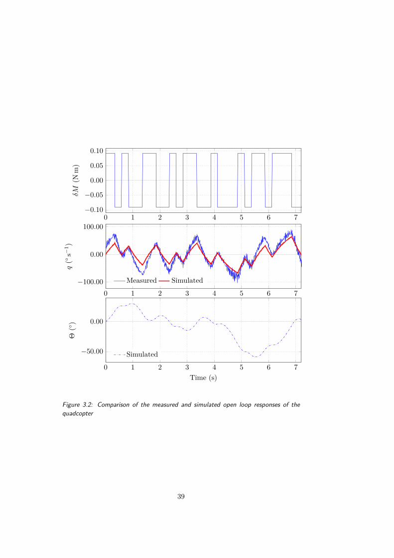
Using a set of previously acquired input-output data this simplifiedmodel was simulated by passing to the input (δΩ) a Pseudo Random BinarySequence (PRBS). The results of this simulation are show in Figure 3.2.The measured and simulated pitch rates (q) are in agreement even if thesimulated system tends to be slower than the actual quadcopter. The pitchangle was not included in the dataset but the simulated pitch angle wasincluded in the results for completeness.

3.1.2 Mixer Matrix

As discussed in Section 1.3.1, the pitch rate controller is a PID whose outputis the desired pitch moment of the quadcopter. The input of the above model

38

0 1 2 3 4 5 6 7−0.10

−0.05

0.00

0.05

0.10

δM(N

m)

0 1 2 3 4 5 6 7−100.00

0.00

100.00

q(

s−1 )

Measured Simulated

0 1 2 3 4 5 6 7

−50.00

0.00

Time (s)

Θ( )

Simulated

Figure 3.2: Comparison of the measured and simulated open loop responses of thequadcopter

39

however is the difference in speed between the front and rear propellers. Thetranslation from one to the other is devolved to the mixer matrix.

Recall that the mixer matrix relates the vertical thrust T and the momentsL, M and N around, respectively, the pitch, roll and yaw axes to the speedsof all four rotors Ω1, Ω2, Ω3, Ω4 in the following manner

Ω2

1Ω2

2Ω2

3Ω2

4

= χ−1

T

L

M

N

. (3.2)

Considering just the pitch control loop, the only non-null angular mo-mentum term is M . We also know that the real input to the system is thedifference in speed between the front and the rear rotor. This allows us toreduce the mixer to a single scalar:

χ = 66.67 (3.3)

3.1.3 Complete System

With this last piece of missing information the models obtained so far canbe inserted into the pitch control scheme previously presented in Figure 1.3.The mixer matrix and the plant model combined describe the quadcopterdynamics from the controller output to the pitch rate and the pitch angle isproduced by the integrator. The resulting control scheme is shown in Figure3.3.

PD PID χ G 1s

Θ0 eΘ q0 eq δM δΩP q Θ−−

Figure 3.3: Control Scheme used to simulate the pitch dynamics

The task now is to choose appropriate reference models.

40

3.2 Structure of the Reference Models

The choice of the reference model is critical to VRFT, the model should befast enough to obtain the best possible bandwidth without being unachievable,but there is no need to rely on complex models to obtain satisfying levels ofperformance. A second order model has been a good starting point. Thisis the simplest class of models that allows us to tune both its static gainand its bandwidth and it can also be easily extended to account for knownproperties of the system such as delays.

If we were to choose the reference models without any knowledge of theplant we would be reduced to semi-random guessing. The knowledge of theplant that we have can be used to guide our decisions and hopefully choose areference model that better represents the actual closed loop transfer functionof the plant.

VRFT also provides for a user-defined weighting function to emphasizeperformance in certain bands of interest. For simplicity all bands wereconsidered of equal importance and the inner and outer weighting functionswere defined as, respectively, Wi(z) = 1 and Wo(z) = 1.

3.2.1 Inner Reference Model

The reference model for the inner loop derives from a second order model.It was observed algebraically that, considering a PID controller and a firstorder plant model G such that

PID(s) = Ki

Kp

1 + s

s, G(s) = a

b + s(3.4)

the resulting closed loop transfer function would be of the form

F (s) = µ1 + s

s2 + cs + d(3.5)

and, to compensate for this additional zero, it was decided to add a zero tothe reference model. This zero was chosen to be in the neighbourhood of thezero naturally emerging from the PID controller for a reasonable range ofPIDs. The resulting form of the inner reference model is thus

41

Mi(s) =ω2

ni

s2 + 2ζiωnis + ω2ni

s + z0z0

(3.6)

where ωni is the bandwidth of the reference model, ζi is the damping ratioand z0 is the position of the zero.

Initially the specific bandwidth and damping ratio of the reference modelwere set to achieve similar performance to what had been observed withthe pre-existing H∞ controller. During the experimental phase the referencemodel would be further tuned to extract better performance from the system.

3.2.2 Outer Reference Model

The structure of the outer reference model was assigned in a similar fashion.It was observed that the closed loop transfer function of the system could beapproximated with a second order system without any additional poles orzeroes.

Mo(s) =ω2

no

s2 + 2ζoωnos + ω2no

(3.7)

where ωni is the bandwidth of the reference model and ζi is the dampingratio.

3.3 Controller Families

The final choice to be made is the choice of the family of controllers to tune.As discussed in Section 1.3.1 the pitch rate controller is a PID whilst thepitch angle controller is a PD.

PD(s) = Kpo + Kdos

Tf s + 1

PID(s) = Kpi + Kii

s+ Kdi

s

Tf s + 1

(3.8)

VRFT requires that the controller family expressed as a vector of lineartransfer functions β(z) such that the parametrised controller is

42

C(z; θ) = βT (z)θ (3.9)

where θ is the parameter vector. This requirement that the controller familybe linear in the parameters means that Tf , the filter time constant of thederivative terms cannot be tuned by the VRFT but must be set beforehand.In the previous H∞ controller the filter time constant was manually set toTf = 0.01 and this value was left unchanged.

The controllers written as vectors of linear transfer functions are

PID(s) =[1 1

s s]

θi

PD(s) =[1 s

]θo

(3.10)

where θi and θo are, respectively, the parameter vectors for the inner andouter controllers.

3.4 Simulation Results

Before starting the testing campaign it was decided to validate the applica-bility of the VRFT approach to the problem of pitch control with a set ofsimulations. Initially, reference models for the inner and outer loops weredeveloped that mimicked the behaviour of the pre-existing H∞ controllers.

One such pair on inner and outer reference models is

MRi(s) = 64s + 320s2 + 72s + 320

MRo(s) = 16s2 + 7.2s + 16

(3.11)

where the inner reference model (MRi) has a bandwidth of 8 rad s−1 and adamping ratio of 0.9 and the outer reference model (MRo) has a bandwidthof 4 rad s−1 and a damping ratio of 0.9.

The VRFT algorithm, applied with the above reference models producedcontrollers with the parameters shown in Table 3.1.

A closed loop simulation of the controllers was performed to ensure thatthe closed loop performance of the system is sufficiently close to the the

43

Inner Controller (PID) Outer Controller (PD)

Kpi Kii KdiTf Kpo Kdo Tf

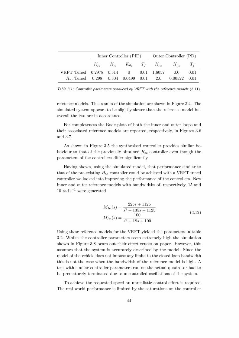
VRFT Tuned 0.2978 0.514 0 0.01 1.6057 0.0 0.01H∞ Tuned 0.298 0.304 0.0499 0.01 2.0 0.00522 0.01

Table 3.1: Controller parameters produced by VRFT with the reference models (3.11).

reference models. This results of the simulation are shown in Figure 3.4. Thesimulated system appears to be slightly slower than the reference model butoverall the two are in accordance.

For completeness the Bode plots of both the inner and outer loops andtheir associated reference models are reported, respectively, in Figures 3.6and 3.7.

As shown in Figure 3.5 the synthesised controller provides similar be-haviour to that of the previously obtained H∞ controller even though theparameters of the controllers differ significantly.

Having shown, using the simulated model, that performance similar tothat of the pre-existing H∞ controller could be achieved with a VRFT tunedcontroller we looked into improving the performance of the controllers. Newinner and outer reference models with bandwidths of, respectively, 15 and10 rad s−1 were generated

MRi(s) = 225s + 1125s2 + 135s + 1125

MRo(s) = 100s2 + 18s + 100 .

(3.12)

Using these reference models for the VRFT yielded the parameters in table3.2. Whilst the controller parameters seem extremely high the simulationshown in Figure 3.8 bears out their effectiveness on paper. However, thisassumes that the system is accurately described by the model. Since themodel of the vehicle does not impose any limits to the closed loop bandwidththis is not the case when the bandwidth of the reference model is high. Atest with similar controller parameters run on the actual quadrotor had tobe prematurely terminated due to uncontrolled oscillations of the system.

To achieve the requested speed an unrealistic control effort is required.The real world performance is limited by the saturations on the controller

44

0 5 10 15 20 25 30 35 40

−20.00

−10.00

0.00

10.00

20.00

Θ(r

ad)

0 0.5 1 1.5 2 2.5 3 3.5 4 4.5 50.00

5.00

10.00

Time (s)

Θ(r

ad)

Set Point Reference Model Out Simulated Pitch Angle (Θ)

Figure 3.4: Comparison of the responses of the outer reference model MRo and theclosed loop transfer function of the system with the controllers of Table 3.1. The upperplot shows the complete simulation whilst the lower plot shows a zoomed-in view ofthe first step.

45

0 5 10 15 20 25 30 35 40

−20.00

−10.00

0.00

10.00

20.00

Θ(r

ad)

0 0.5 1 1.5 2 2.5 3 3.5 4 4.5 50.00

5.00

10.00

Time (s)

Θ(r

ad)

Set Point Θ - H∞ Θ - VRFT

Figure 3.5: Comparison of the responses of the closed loop transfer function of thesystem with the VRFT tuned controllers and the pre-existing H∞ controllers with theparameters of Table of Table 3.1. The upper plot shows the complete simulation whilstthe lower plot shows a zoomed-in view of the first step.

46

100 101 102 103−40.00

−20.00

0.00

Mag

.(d

B)

100 101 102 103−90.00

0.00

ω(rad)

Phas

e( )

Reference Model Closed Loop

Figure 3.6: Comparison of the Bode plots of the inner reference model MRi and theclosed loop transfer function for the pitch rate regulation loop with the controllers ofTable 3.1.

100 101 102 103−100.00

−50.00

0.00

Mag

.(d

B)

100 101 102 103−180.00

−90.00

ω(rad)

Phas

e( )

Reference Model Closed Loop

Figure 3.7: Comparison of the Bode plots of the outer reference model MRo and theclosed loop transfer function for the pitch angle regulation loop with the controllers ofTable 3.1.

47

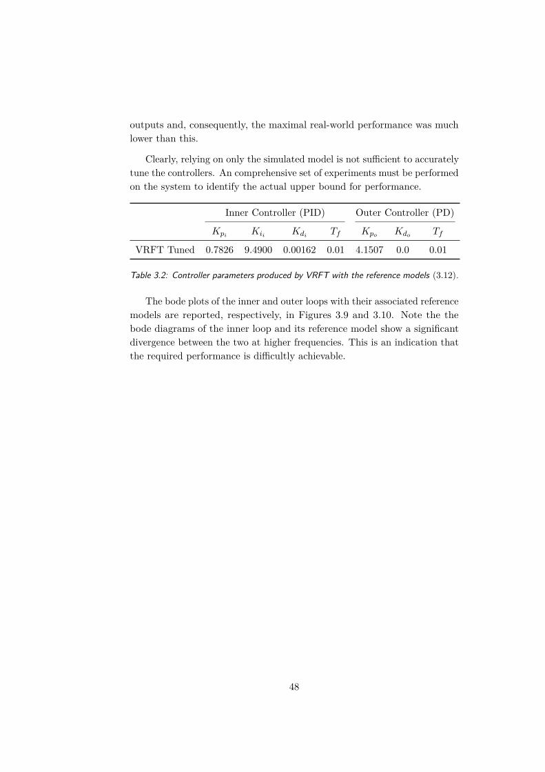
outputs and, consequently, the maximal real-world performance was muchlower than this.

Clearly, relying on only the simulated model is not sufficient to accuratelytune the controllers. An comprehensive set of experiments must be performedon the system to identify the actual upper bound for performance.

Inner Controller (PID) Outer Controller (PD)

Kpi Kii KdiTf Kpo Kdo Tf

VRFT Tuned 0.7826 9.4900 0.00162 0.01 4.1507 0.0 0.01

Table 3.2: Controller parameters produced by VRFT with the reference models (3.12).

The bode plots of the inner and outer loops with their associated referencemodels are reported, respectively, in Figures 3.9 and 3.10. Note the thebode diagrams of the inner loop and its reference model show a significantdivergence between the two at higher frequencies. This is an indication thatthe required performance is difficultly achievable.

48

0 5 10 15 20 25 30 35 40

−20.00

−10.00

0.00

10.00

20.00

Θ(r

ad)

0 0.5 1 1.5 2 2.5 3 3.5 4 4.5 50.00

5.00

10.00

Time (s)

Θ(r

ad)

Set Point Reference Model Out Simulated Pitch Angle (Θ)

Figure 3.8: Comparison of the responses of the outer reference model MRo and theclosed loop transfer function of the system with the controllers of Table 3.2.

49

100 101 102 103

−30.00−20.00−10.00

0.00M

ag.

(dB

)

100 101 102 103−90.00

0.00

ω(rad)

Phas

e( )

Reference Model Closed Loop

Figure 3.9: Comparison of the Bode plots of the inner reference model MRi and theclosed loop transfer function for the pitch rate regulation loop with the controllers ofTable 3.2.

100 101 102 103−80.00−60.00−40.00−20.00

0.00

Mag

.(d

B)

100 101 102 103−180.00

−90.00

0.00

ω(rad)

Phas

e( )

Reference Model Closed Loop

Figure 3.10: Comparison of the Bode plots of the outer reference model MRo and theclosed loop transfer function for the pitch angle regulation loop with the controllers ofTable 3.2.

50

Chapter 4

Experimental Results

In chapter 3 the performance of the simulated system was explored and it wasshowed that, since the model does not account for non-linearities and othercomplex effects, it is possible (at least theoretically) to achieve unrealisticlevels of performance. Tests on the real hardware were conducted in orderto find an actual bound to the achievable performance.

In Section 4.1 the actual components of the quadcopter will be detailed. InSection 4.2 the fashion in which the required input-output data was collectedwill be explained. VRFT has provisions for noise mitigation procedures.Their use will be detailed in Section 4.3. In Section 4.4 the reference modelsused for the VRFT will be shown and, finally, in Section 4.5 the results of theactual experiments on the system will shown and compared to a pre-existingmanually tuned H∞ controller.

4.1 Quadcopter Hardware & Firmware

The quadcopter used for this work was entirely developed at Politecnico diMilano based on the following requirements:

• X frame of medium size (450 to 550 mm distance between oppositerotors)

• Overall weight of less than 2 kg

• Payload of at least 0.5 kg

• Flight time of at least 10 minutes

51

The specifications of the components chosen in order to achieve thesegoals are documented in the following sections. A fixed-pitch actuationscheme was retained since the performance requirements of the system arerelatively low. For a more detailed explanation behind these choices see [5]

4.1.1 Frame

The frame (Figure 4.1a) is the central building block of the quadcopter. TheTalon V2.0 frame, built out of carbon fibre and aluminium was retained dueto its low weight and high strength. The distance between opposite motorson this frame is 500 mm.

4.1.2 Motors, ESC & Propellers

The motors (Figure 4.1b) are brushless DC motors (BLDC) from the RCTimerHigh Performance series (HP2814). Since brushless motors are synchronousthey cannot be driven by a simple DC current but require an inverter toprovide a switching electric signal. This is the Electronic Speed Controller(ESC). In this case, the RCTimer NFS ESC 30A (Figure 4.1c). This com-bination of motor and driver is able to push the propeller to close to 8000rpm

The propellers mounted on the motors have two 12 inch blades with a4.5 pitch angle (Figure 4.1d).

4.1.3 Battery

The batteries used on the quadrotor are Turnigy nano-tech 4000 mA h. Theseare LiPo 3 cell batteries with a nominal tension of 3.7 V per cell for a totaltension of 11.1 V per battery. The batteries are capable of supplying aconstant current of 100 A with peaks of up to 200 A for short periods oftime.

4.1.4 Vibration Damping

To reduce the mechanical vibrations transmitted through the frame from themotors a support plate onto which the electronics are mounted was realised

52

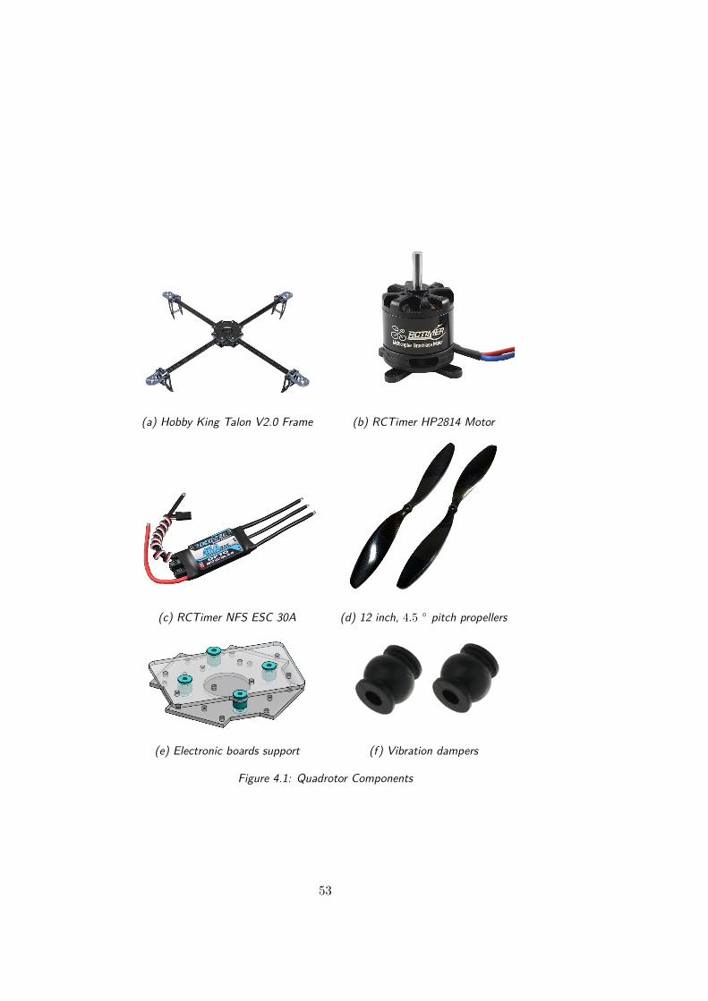
(a) Hobby King Talon V2.0 Frame (b) RCTimer HP2814 Motor

(c) RCTimer NFS ESC 30A (d) 12 inch, 4.5 pitch propellers

(e) Electronic boards support (f) Vibration dampers

Figure 4.1: Quadrotor Components

53

(Figure 4.1e). This plate is then fixed to the frame with vibration dampingrubber feet (Figure 4.1f).

4.1.5 Flight Control Unit & Firmware

The flight control unit is the brains of the quadrotor. It was implementedon a Rapid Robot Prototyping (R2P) boards [1]. This is an open sourcehardware and software framework that enables the rapid development ofrobotic applications. These boards implement an IMU, serial communication,control of the RC motors with PWM signals and the actual flight control.The modules use a publish/subscribe architecture to communicate.

The control portion is implemented in Simulink and compiled to C++code. The firmware manages the communication between the sensors andthe generated code in order to control the quadcopter.

4.1.6 Test Bed

All the tests on the quadrotor were performed on a test bed that constrainsall translational degrees of freedom as well as the roll and yaw motions.Only the pitch rotation is left unconstrained. This ensures that the tests arerepeatable and safe and that an erroneous choice of the controller parameterswill not send the system crashing through the room.

(a) Test Bed, Front View (b) Test Bed, Top view

The test bed is built out of x-frame aluminium rods and weighted withsacks of concrete. The upper part of the frame has a smooth rod resting onball bearings at each extremity for frictionless rotation. The quadrotor is

54

then securely fastened to this rod.

In the current mounting scheme the rod passes as close as possible tothe centre of mass of the system in order to interfere as little as possiblewith the dynamics of the quadrotor. Because of the physical configuration ofthe system there is small distance between the rod and the actual centre ofmass. In turn, this causes the system to act like a very small pendulum andthe test bed adds some damping when the system quadrotor achieves higherpitch angles. In practice this damping is negligible for small oscillations.

The test bed holds the quadcopter high enough that ground effect dis-turbances are avoided however, since the test takes place in a closed spacesome recirculation of rotor wakes occurs. This represents a discrepancy whencompared to outdoor flight conditions where the rotor wakes develop freefrom obstacles. Even so, it has been shown in previous work that such a testbed is representative of actual attitude dynamics in flight.

4.1.7 Additional Flight Hardware

The quadcopter also holds a RaspberryPi 2 board used to interface the R2Pmodules with a ROS network but this functionality was unused for the tests.In addition a small ultrasonic sensor has been mounted on the drone tomeasure the distance from the ground when landing.

4.2 Tuning Experiment

The most important pre-requisite for data-driven algorithms such as VRFT isthe collection of a sufficiently long persistently exciting input-output dataset.

Since the aim of this work is to tune the controllers on the pitch regulationloop all the tests were performed on the test bed described in Section 4.1.6.The test bed constrains all the degrees of freedom of the vehicle except thepitch rotation.

The control scheme for the pitch control loop is shown in Figure 4.3. SeeSection 1.3.1 for a detailed description of each component and the symbolsused.

In the cascade VRFT setting the system should be divided into fourparts: an inner and an outer parametrised controller and and inner and

55

PD PID χG 1s

Inner Plant Outer Plant

Θ0 δM q Θ−−

Figure 4.3: Control scheme for VRFT as applied to the pitch control loop where q, thepitch rate of the quadcopter, is analogous to the inner output signal yi, Θ, the pitchangle, is analogous to the outer output signal yo and δΩP , the change in speed of thepropellers, is analogous to the plant input signal u.

anouter unknown plant. The controllers are quite obviously the PD andPID blocks in Figure 4.3. It follows that the χG blocks representing thedynamics from the requested torque around the pitch axis to the pitch rateis the inner plant and the integrator 1

s computing the pitch angle from thepitch rate is the outer plant.

The experiments used to gather the input-output data should be per-formed in open loop, providing the torque δM as an input and reading thepitch rate q and the pitch angle Θ as the inner and outer outputs yi andyo. Unfortunately the firmware does not allow us to provide δM as an inputdirectly or read the pitch angle Θ when operating in open loop conditions.Instead we were only able to specify as the input δΩP the difference in thespeed of the front and read propellers and read he pitch rate q as the singleoutput.

This is not an issue however since, as shown in Section 3.1.2, the mixer,considering only the pitch control loop, is a known scalar. Consequently, theinner plant input could be computed quite simply from the available data as

δM = χ−1δΩP . (4.1)

The pitch angle , Θ, the output of the outer plant, can also be calculatedalgebraically. Whilst in the general case the outer plant model is unknown,in our case the it is an integrator. The pitch angle Θ is simply the integralof the pitch rate q over time. Consequently we were able to calculate thepitch angle as

Θ =∫ t

0q dt (4.2)

56

With the quadcopter firmware operating in open loop, a Pseudo RandomBinary Sequence (PRBS) was generated for the input δΩP and fed into thesystem with a time step of 0.01s. This sequence was generated in such wayas to reliably excite the dominant dynamics of the system. This input signaland the computed torque around the pitch axis δM are show in Figure 4.4.

0 1 2 3 4 5 6 7

−5.00

0.00

5.00

δΩP

(rad

s−1 )

0 1 2 3 4 5 6 7−0.10

0.00

0.10

Time (s)

δM(N

m)

Figure 4.4: Measured δΩP and computed control variable δM . Measured signals arerepresented with a continuous line, computed signals are shown with a dotted line

The output measurement, the pitch rate signal q, was acquired and loggedby the quadcopter itself using its on-board IMU with a time step of 0.01s.The pitch angle Θ was computed from the pitch rate measurements as shownin equation (4.2). The measured pitch rate and the computed pitch angleare shown in Figure 4.5.

4.3 Noise Considerations

Like all real world signals the input-output signals measured on the quad-copter are noisy. As detailed in Section 2.3.3, VRFT solves the problem ofreducing the noise induced bias in the criterion it minimises with an instru-mental variable approach. This requires either the collection of a secondinput-output dataset or the identification of a high-order model of the plant

57

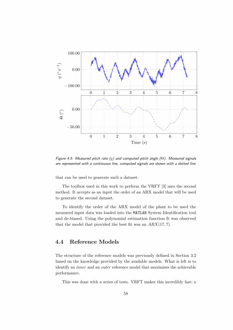
0 1 2 3 4 5 6 7 8−100.00

0.00

100.00q

(s−

1 )

0 1 2 3 4 5 6 7 8

−50.00

0.00

Time (s)

Θ( )

Figure 4.5: Measured pitch rate (q) and computed pitch angle (Θ). Measured signalsare represented with a continuous line, computed signals are shown with a dotted line

that can be used to generate such a dataset.

The toolbox used in this work to perform the VRFT [3] uses the secondmethod. It accepts as an input the order of an ARX model that will be usedto generate the second dataset.

To identify the order of the ARX model of the plant to be used themeasured input data was loaded into the MATLAB System Identification tooland de-biased. Using the polynomial estimation function It was observedthat the model that provided the best fit was an ARX(17, 7).

4.4 Reference Models

The structure of the reference models was previously defined in Section 3.2based on the knowledge provided by the available models. What is left is toidentify an inner and an outer reference model that maximises the achievableperformance.

This was done with a series of tests. VRFT makes this incredibly fast; a

58

single input-output dataset can be used to tune any number of controllers.Once programmed onto the quadcopter the system was put through a seriesof step inputs and any controllers that unexpectedly yielded unstable controlloops were immediately discarded to avoid what Elon Musk famously referredto as rapid unscheduled disassembly events. The final choice of parametersrepresents the best trade-off between the rise time and the settling time.

This also illustrates one of the limitations of VRFT: it does not provideany kind of guarantee that the closed loop transfer function will be stable.

4.4.1 Inner Reference Model

The structure of the inner reference model decided in Section 3.2.1 is

Mi(s) =ω2

ni

s2 + 2ζiωnis + ω2ni

s + z0z0

where ωni is the bandwidth of the reference model, ζi is the damping ratioand z0 is the position of the zero.

At the conclusion of the testing campaign I observed that the best tradeoffbetween the rise time and the settling time was obtained with a bandwidthωni = 8rad s−1, a damping-ratio ζi = 0.9 and a zero placed in z0 = 5

Mi(s) = 64s + 3205s2 + 72s + 320

s − 55 (4.3)

The VRFT procedure is defined only for discrete time systems but thequadcopter firmware considers only continuous time models. This mismatchwas overcome by discretising the models prior to performing the VRFT andconverting the output back to a continuous time model.

The discretised form of the inner reference model, considering a time stepTs = 0.01s is

MRi(z) = 0.1221z − 0.1162z2 − 1.86z + .8659 . (4.4)

59

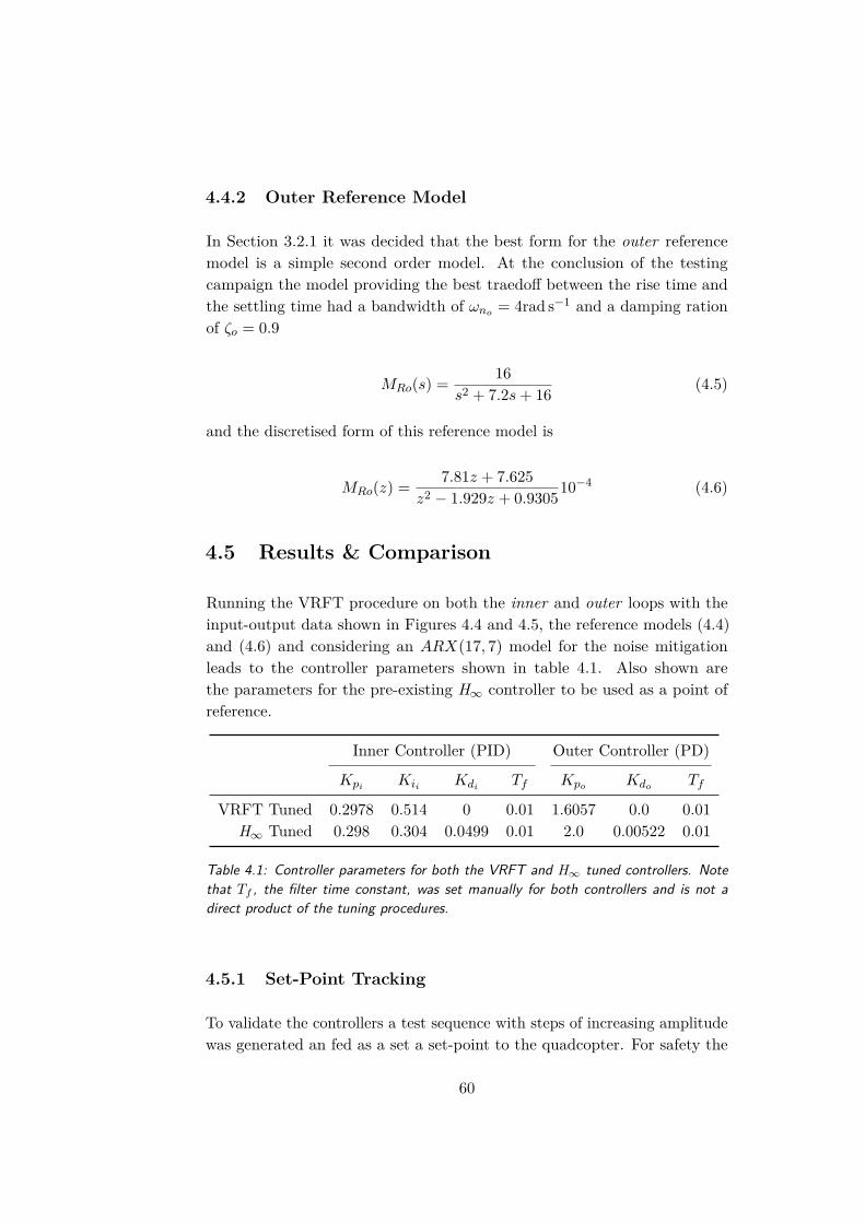
4.4.2 Outer Reference Model

In Section 3.2.1 it was decided that the best form for the outer referencemodel is a simple second order model. At the conclusion of the testingcampaign the model providing the best traedoff between the rise time andthe settling time had a bandwidth of ωno = 4rad s−1 and a damping rationof ζo = 0.9

MRo(s) = 16s2 + 7.2s + 16 (4.5)

and the discretised form of this reference model is

MRo(z) = 7.81z + 7.625z2 − 1.929z + 0.930510−4 (4.6)

4.5 Results & Comparison

Running the VRFT procedure on both the inner and outer loops with theinput-output data shown in Figures 4.4 and 4.5, the reference models (4.4)and (4.6) and considering an ARX(17, 7) model for the noise mitigationleads to the controller parameters shown in table 4.1. Also shown arethe parameters for the pre-existing H∞ controller to be used as a point ofreference.

Inner Controller (PID) Outer Controller (PD)

Kpi Kii KdiTf Kpo Kdo Tf

VRFT Tuned 0.2978 0.514 0 0.01 1.6057 0.0 0.01H∞ Tuned 0.298 0.304 0.0499 0.01 2.0 0.00522 0.01

Table 4.1: Controller parameters for both the VRFT and H∞ tuned controllers. Notethat Tf , the filter time constant, was set manually for both controllers and is not adirect product of the tuning procedures.

4.5.1 Set-Point Tracking

To validate the controllers a test sequence with steps of increasing amplitudewas generated an fed as a set a set-point to the quadcopter. For safety the

60

tests were performed with the quadcopter securely fastened to the test-bed.The result of one such run with the VRFF tuned controllers of Table 4.1 areshown in Figure 4.6.

0 5 10 15 20 25 30 35 40

−20.00

0.00

20.00

Θ( )

0 2 40.00

5.00

10.00

Time (s)

Θ( )

20 22 240.00

10.00

20.00

Time (s)

Figure 4.6: Pitch angle set point tracking using the VRFT tuned controller

The test was repeated 10 times using . the both the VRFT and H∞tuned controllers and the average mean square error was computed.

The set-point tracking performance of the quadcopter with, respectively,the VRFT and H∞ controllers during one, randomly chosen, run is shownin Figures 4.6 and 4.7.

The VRFT and H∞ tuned controllers were very similar in the simula-tion runs with the VRFT controller being marginally slower than the H∞controller. In these experiments this trend is inverted. The VRFT tunedcontroller is marginally faster than the H∞ controller. This can be explainedquite easily: the H∞ tuned controller is based on an identified model of thesystem and can only ever be as good as the identified model. The VRFTtuned controller has the advantage of being tuned on real data collected onthe system and is thus exempt from modelling errors.

The mean square error, comparing the measured pitch angle to the set-point, was computed for each test and averaged. The values for the VRFTand H∞ tuned controllers are shown in the first column of table 4.2. The

61

0 5 10 15 20 25 30 35 40

−20.00

0.00

20.00Θ

( )

0 2 4

0.00

5.00

10.00

Time (s)

Θ( )

20 22 24

0.00

10.00

20.00

Time (s)

Figure 4.7: Pitch angle set point tracking using the pre-existing H∞ controller

mean square error of the VRFT controller, whilst a little higher than that ofthe H∞ controller is still within acceptable bounds. It can be explained bythe slightly more oscillatory nature of the VRFT tuned controller.

4.5.2 Disturbance Rejection

The disturbance rejection properties of the firmware were considered usinga similar method. The firmware of the quadcopter provides a method tointroduce a step disturbance on the speed of the motors. This was usedto repeatedly reduce the lift generated by the motors on the front of thequadcopter (motors 1 & 2) by 10 %. The test was repeated 10 times withboth the VRFT and H∞ tuned controllers and the average of the meansquare error was computed.

The disturbance rejection performance of the quadcopter with, respec-tively, the VRFT and H∞ controllers during one, randomly chosen, run areshown in Figures 4.7 and 4.7.

It is immediately apparent that the VRFT tuned controller offers sig-nificant improvements to the steady state error. The H∞ tuned controllersettles with a steady state error of several degrees whereas the VRFT tuned

62

0 2 4 6 8 10 12 14 16 18 20 22 24

−20.00

0.00

20.00

Dis

turb

.(%

)

0 2 4 6 8 10 12 14 16 18 20 22 24

0.00

0.50

1.00

Time (s)

δM(N

m)

Figure 4.8: Disturbance rejection properties of the VRFT Tuned controller. The dis-turbance is a 10% drop in the speed of rotors 1 & 2.

0 2 4 6 8 10 12 14 16 18 20 22 24

−20.00

0.00

20.00

Dis

turb

.(%

)

0 2 4 6 8 10 12 14 16 18 20 22 24

0.00

0.50

1.00

Time (s)

δM(N

m)

Figure 4.9: Disturbance rejection properties of the H∞ Tuned controller. The distur-bance is a 10% drop in the speed of rotors 1 & 2.

63

controller achieves zero state error. In addition the control effort requiredby both controllers is quite similar even if the VRFT tuned controller hasslightly higher peaks.

The improvement is reflected in the steady state error of the two con-trollers as shown in Table 4.2. The mean square error of the VRFT tunedcontroller is slightly lower than that of the H∞ controller.

Mean Square Error

VRFT Tune Controller H∞ Tuned Controller

Undisturbed 10.719 6.3384Disturbed 4.7908 5.5686

Table 4.2: Mean of MSE for validation experiments considering both VRFT and H∞tuned controllers

64

Bibliography

[1] Andrea Bonarini, Matteo Matteucci, Martino Migliavacca, and DavideRizzi. “R2P: An open source hardware and software modular approachto robot prototyping”. In: Robotics and Autonomous Systems (2014).issn: 09218890. doi: 10.1016/j.robot.2013.08.009.

[2] M C Campi, A Lecchini, and S M Savaresi. “Virtual reference feedbacktuning: a direct method for the design of feedback controllers”. In:Automatica 38 (2002), pages 1337–1346. url: www.elsevier.com/locate/automatica.

[3] Marco Campi and Sergio Savaresi. VRFT Toolbox for MATLAB. url:http://marco-campi.unibs.it/VRFTwebsite/.

[4] Simone Formentin, Alberto Cologni, Damiano Belloli, Fabio Previdi,and Sergio M. Savaresi. “Fast tuning of cascade control systems”. In:IFAC Proceedings Volumes (IFAC-PapersOnline). 2011. doi: 10.3182/20110828-6-IT-1002.02761.

[5] Mattia Giurato. “Design, integration and control of a multirotor UAVplatform”. Master’s thesis. Politecnico Di Milano, 2015. url: http://hdl.handle.net/10589/115191.

[6] Htikan Hjalmarsson, Michel Gevers, Svante Gunnarsson, and OlivierLequin. “Iterative feedback tuning: Theory and applications”. In: IEEEControl Systems Magazine (1998). doi: 10.1109/37.710876.

[7] Pietro Panizza, Davide Invernizzi, Fabio Riccardi, Simone Formentin,and Marco Lovera. “Data-driven attitude control law design for avariable-pitch quadrotor”. In: Proceedings of the American Control Con-ference. 2016. doi: 10.1109/ACC.2016.7525620.

[8] Klaske Van Heusden, Alireza Karimi, and Dominique Bonvin. “Data-driven model reference control with asymptotically guaranteed stability”.In: International Journal of Adaptive Control and Signal Processing(2011). issn: 08906327. doi: 10.1002/acs.1212.

65