●

.

REMOTE SENSING DATA ACQUISITION,ANALYSIS RND ARCHIVAL

by

William J. Stringer

FOURTH QUARTERLY REPORT

Dctober i - December 31, 19B6,..

OCSEFIP: F&arch Unit k“ &-$

Submitted to

National Oceanic & Atmospheric Administration. Clcein Assessments Division

, Alaska Dffice..., PO,, B9X 36 . .Anchorage, Alaska 9951”3

February 19S7

Genphysi cal InstituteUniversity of Alaska

Fairbanks, 91 aska 99775-0S00

i

.

r ,

FOURTH QUARTERLY REPORTOctober 1 - December 31, 1986

OCSEAP Research Unit 267Contract #50ABNC 600041

ACTIVITIES THIS QUARTER

1. Assistance to RU 625 (J. Brueggeman ) . This studyoccupied the bulk of our activities during this quarter. Thework consisted of providing ice-related data which could be usadin conjunction with Brueggeman’s whale sightings in the BeringSea. The whale sightings (about 3, 000) have been coded in termsof latitude and longitude. The objective of our efforts was toprovide data which could be used to determine whether ameaningful statistical relationship could ba found between thesesightings and ice parameters such as concentration, type(thickness ) and ice edge location ( including pal ynya boundaries ) .

Fortunately the software which had been developed for ourongoing polynya analysis as well as some of the digital palynyaboundaries could be used for this analysis. However, it wasnecessary to digitize additional data from the years alreadyanalyzed as well as data from years which had not yet beendigitized for polynya analysis.

Specifically, the newly digitized data consisted of thefollowing:

1. Data for the Anadyr Polynya was added. We had notpreviously digitized this polynya because it liesbeyond the NOAA-OCSEAP O .S. study area. However, thewhales are international travelers so this data setneeded to be added. Data for January, February, Marchand April of 1978 and 19S3 were added to existing filesand new files were created for data for January 1986.

2. The Bering Sea ice edge far January, February, March,and April of 1979 and 1983 was added mostly to existingfiles. However, for a few dates new files werecreated. Entirely new files were created for January1986.

Material delivered to Brueggemen at the end of this quarterconsisted of:

1) Magnetic tape captaining all files of Bering Sea iceand Anadyr, St. Lawrenca Island, and St. MatthewsIsland polynyas.

,

2) Print-out maps of the data set described in 1 ) above.

!, ,I I

3] Tabular print-outs of arsal extant and perimeterlengths of polynyas listed above as well as otherpalgnyas which occasional 1 y occur within the studyarea.

4) Tabular evaluation of ice conditions at 113 specifiedlocations representing whale sightings and lncations ofno whale evidence. (This was essentially a trial runfor a larger follow-on project which is described in“Next Quarter Activities. ”

The above materials were delivered to Brueggeman’s researchunit during an on-site working visit by Richard Grotefendt,Brueggeman’s assistant.

2. Polynya Analysis. Despite the diversinn of effort tothe whale studies, some progress was reads in the study of polynyasize. Three additional years’ data were digitized: 1977, 1979,and 1983, including the Anadyr pol ynya. In addition, the Anadyrpolynya was added to the data for 1975 and 1986. Our previouswork on the statistics of the Chukchi Sea resulted in tbeidentification of 1979 and 1983 as relative maximum and minimumyears of open water. Hence these are interesting years’ data forcomparison purposes.

Although we have not yet digitized all the years’ dataavailable to us, we decided to at least start examining theresults in arder to begin identifying the mast useful andmeaningful analysis functions. As a first step in this directionit was determined to calculate median polynya values for fourmajor polynya systems as a function of month.

This has turned out to be a useful exercise because we havehad to confront several cnncepts related to palynyas. As abackground, it is instructive to first consider the WorldMeteorological Organization definition of a polynya - ‘anirregularly shaped opening enclosed by ice. As opposed to afracture, the sides of a polynya could not be refitted to form auniform ice sheet. Palynyas may contain brash ice or uniformlythinner ice than the surrounding ice. a Thus, areas of thin ice

. surrounded by thicker ice may be considered pol ynyas. Very oftenon satellite imagery polynyas can be seen with areas of obviouslyopen water general 1 y surrounded by ice but on the down-wind sidethe transition f ram water to ice is often fairly uniform and itis difficult to determine where to draw the polynya boundary inthis area. We have taken the boundary to be the transitionbetween dark gray and light gray (an ice thickness of around10cm) . However, in many cases this determination is a bitarbitrary. In any case, this is the definition we have used indetermining what constitutes a polynya.

.

The size of polynyas is interesting from the considerationof salt and en’ecgy budgats for tbe water bodies which contain

2

. .

.>

—

them. And, if one is considering the long term effacts of themphenomena polynya size as a function of time is a criticalmeasure. However, satellite measurements that depend on cloud-free conditions are by nature irregular in frequency andtherefore, same scheme must be utilized to transform measurementsmade at irregular intervals into measures at regular intervals.

One logical approach to this transformation is to determinea measure of a central tendency far the quantity in question overperiods sufficiently long to contain several measurements butsufficiently short to represent a characteristic period of time.In our case, we chose a month as a characteristic period,implying that any one measure within the month was as good as anyother ( i .e. statistical trends of less than a month’s durationare not significant) . Of course there is another tacitunderstanding here; that each measure is statisticallyindependent. To accomplish this, the measurements should besufficiently separated that they da not essential lY represent twomeasures of the same value. The satallite data are inherentlyseparated by one day at a minimum. Although we have assumed thatthis is sufficient temporal separation for an independentmeasurement, we may need to address this question in detaillater.

The next topic for consideration is the measure of centraltendency to be employed. Of the three, average, median and mode,we chose median for the following reasons. In some casespolynyas join to the open ocean or other palynyas for a while.What is their area then, and what does “area” mean in this case?The polynyas can ‘t be ignored in these cases and therefore simplydeleting the observation f ram the data set is statisticallyunsound. On the other hand, so is adding an arbitrari lY largenumber to a set to be averaged. For this reason we did not takean average value. Mode iS difficult to determine for a limiteddata set and would tend to emphasize values from strings of datafrom short time periads within the month - just the sort of datawe would wish to reemphasize. Median values on the other hand,are nat unduly influenced by a few arbitrarily large values atone end of the data set and tend to deemphssize the importance ofcontinuous strings of data ( provided they are short compared tothe entire data set ) . ‘Therefore, we have chosen to determinemedian monthly values of polynya sizes.

However, this is not the end of the need for definitions.We soon realized that ‘polynya size- means size of an existingpolynya. Thus one could argue that times when the polynyalocation was frozen or the polynya open to the ocean on one sidecould arguably be deleted from the data set if one is interestedin the actual size of the palynya. On the other hand, as ameasure of a process such as salt rejection during freezing, thefact that the palynya is frozen over or completely open is ofgreat importance. Therefore, for this pilot study, we calculatedmedian polynya sizes based on both data set definitions.Finally, we have listed the maximum polynya size observed during

3

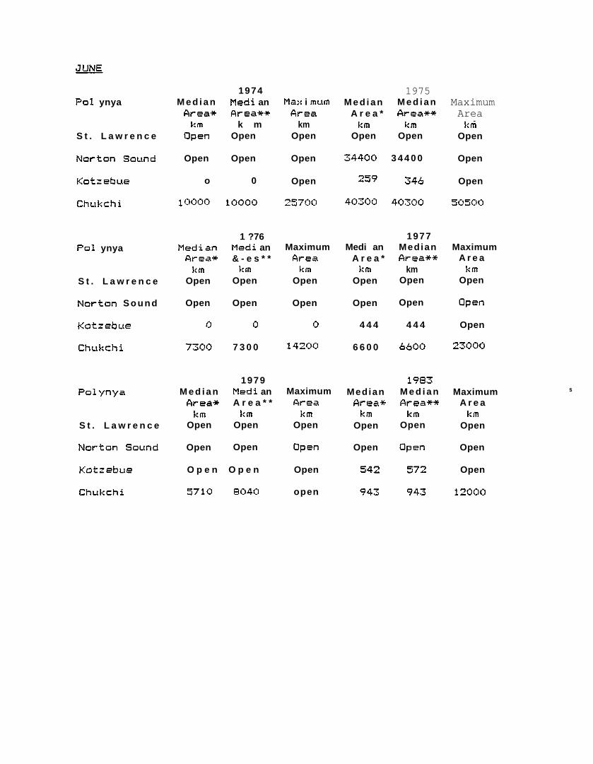
each month to give come indication of the variability in polynyasize which occurred during the manth. These results are shown inTable I.

Table I lists polynya median sizes by month for 1974 (exceptJanuary and February) , 1975, 1977, 1979, 1983 and 1986 using bothdata set definitions for median determination, and maximumpolynya size for the first 6 months of each year. The polynyas1 isted are defined by Table 2 and Figure 1.

Figure 1 is a map showing the approximate location ofpersistent polynyas in the study area where they are given letterdesignations. Table II is the key between the letterdesignations and the name given each polynya. However, two ofthe polynyas for which areas are listed in Table I are actuallyaggregate PO IYnYas Campiled in order to give an idea of tbe totalpolynya areas in the study area. “St. Lawrence” is the sum ofSt. Lawrence, North ( E ) and St. Lawrence, South ( D ) . (However,usually only one is open at a time. ) Norton Sound (K) is thesingle polynya at the eastern end of Norton Sound. Kotzebue (Q)is the polynya which occurs between pack ice and fast ice inouter Kotzebue Sound. Chukchi is the sum of Cape Lisburne -Paint Lay (T), Pt. Lay - Icy Cape (U) and Icy Cape - Pt. Barrow(V] . (Often these polynyas join to fGrm a single polynya - thisphenomenon occurs within a number of pal ynya systems, making thetracking of the size of a designated polynya a tricky matter. )

These data have not been analyzed further. Our plan is toperform a multivariate analysis of polynga sizes versus time.

/“

3. Data Acquisition and Projects Conducted for OCSEAPManagement. We have provided enhanced AVHRR imagery in thevicinity of Kotzebue Sound and in the Beaufort Sea to OCSEAPmanagement. The letters of transmittal - attached as Appendix 1,describe this work.

4. Data Received and Archived. We have continued to obtain —

and archive dai lY NOAA AVHRR satellite imagery of the OCSEAPstudy areas around Alaska. Because of the three-to-four times

I

100fif3

daily coverage of Alaska by these satellites, we cannot possibly AU1+CL.afford to purchase a copy of each at the $10.00 per copy ratecharged. Thus we select only the best images (approximately *three per day and purchase them in positive transparency formatdirectly from the receiving station at Gilmore Creek) . (ourexperience has shown us that positive transparencies retain the “Fhighest information content for analysis and reproductionpurposes of all data formats other than digital tapes. )

In addition to the positive transparency format data, wealso receive hard copy facsimile transmission positive printsthat have been used by the weather service. There 1s a greatquantity of these prints as they represent at least one copy of ,.

4 ?LD2hkti

.

each day’ 3 image and aometimea digital enlargsmsnta andenhancements of particular areas. These are sent to us by theweather service about a month after they are transmitted fromGilmore Creek. We archive these data (although the image qualityis considerably diminished from that of the positivetransparency ) because some feature of interest to OCSEAPinvestigators maY be found on one of these images which did notaPeear on an ima9e judged to be one of the day’s “best” images.Followinq thase critaria, we archived approximately 270 positivatransparencies and 2700 positive facsimile prints this guarter.

Our “Quick-Laok” ground station received a total of 66images from Landsats 4 and 5. This relatively small data set isa result of cloudy weather in late fall and a conscious effort toobtain only useful (relatively cloud-free) imagery. These imagesare often digitally enhanced and enlarged with copies of theseproducts archived as wel 1 as the standard 1: 1!4 scale print. Insome instances we have obtained images at times when the sun wasbelow the horizon - yet ice conditions are easily observed. Thisis an additional value of our ground station and imageenhancement capability.

We also continue ta receive and archive the NOAA/NAVY ice Icharts published weekly and the drifting buoy data published ~monthly by the Polar Ocean Center in Seattle. Finally, this

( %%%quarter we acquired Side-Looking Airborne Radar imagery of theBeaufort Sea as part of a data search (see Appendis II).Normally we only monitor the acquisition of this data because of

s

its limited value and not so 1 imited expense.

ACTIVITIES NEXT QOARTER

1. Assistance to Brueqgeman (RO 625). We are creating aprogram to distinguish whether a given station is within oroutside a polynya from the digitized data. When completed, al 13000 nf Brueggeman’s whale/no whale data wi 11 be tested forcorrelation with polynyas.

2. Polynya Analysis. We will continue our analysis ofpolynya data. Emphasis this quarter will be applied todetermining trends and significance of polynya extent datasimilar to and including the data reported here in Table I.

3. Data Acquisition. We will continue to acquire andarchive Landsat and AVHRR satel 1 ite imagery as well as NOAA/Navyice charts and ice drifting buoy data.

FONDS EXPENDED

As of Oecember 31, 1986 we have expended $101,940 of a totalauthorized $205,799.

5

680!

180. 170’=W 160° W

\

‘l

QST. LAWRENCEISLAND E

D SOUND .“

sT. MATTHEW

&

‘ B ISLANDA. .

NUN IVAKISLANO

1 .. ..-. . . . . . .,,” - w l-u- w

s

Figure 1. Map showing approximate location of persistent polynyasin the Bering Sea/ Chukchi Sea study area.

:,

TABLE I. T a b u l a t i o n of %lynya Area Medians f o r S i x Months o v e rI

Six Year5.

J fiNUARY

1973MedianArea**

km23120

1977Max i mum M e d i a n Pledi an Max i mum

A r e a &rea* A r e a * * f%-eaMedi anArea*

~km

3120

Polynya

km2 k mz k mz kmzS t . L a w r e n c e

N o r t o n S o u n d

Motzebue

Chukchi

218 1610 ~59c) a i 4CI0 3 4 2 0

3940 i i 100 4520 5s20 7s60

c1 o

1979MedianF+rea**

i:mOpen

1983M a x i m u m M e d i a n Median Maximumhrea Area* f i r e s * * Area

km km km kmOpen i ascl 1940 3 4 4 0

Polynya Medi an.%- ea *

kmOpen5t. L a w r e n c e

N o r t o n S o u n d

~OtZebL~e

ChL~kchi

1.570 1700

0 1490 I 49i) c) 1550 4a4cl

7s5 3 8 0 0,

1966Mediani%-es*++km

20(3(]

Pol ynya M e d i a nA r e a *

km~(jclc)

MaximumA r e a

kmi 0500S t . L a w r e n c e

N o r t o n S o u n d

~OtZebLLe

Chukchi

1 SC1O 4 2 3 0

620 17s0

1 0 5 0 i 050 7410

.,

:.

FEEIF(UARY

1975 1 9 7 6Medi an M e d i a n Maximum Medi an M e d i a n

A r e a *Max i mum

A r e a * * (%-es Area* Area+% ~reaF’ol ynya

km km1720 3240

km8533

km7 4 0

km~5713S t . L a w r e n c e

Norton S o u n d

Kotzebue

Chukchi

.564 70s .5Ck50

149001 C1600 I 1>6(:)0 o 6 7 0

15700 15700 3,51 [:)(> ,-.J 0

i 977Median Medi anArea* Area**

km km1640 1640

i979Medi anArea**

km4 5 8 0

Maximum?irea

km~750

MaximumArea

kmi 02(:)0

F’ol ynya

S t . L a w r e n c e

Narton Sound

Kotxebue

Chukchi

788 17600

0 0 c1

1830 33005,540

1983M e d i a n Medi an

Qrea* #W-es**km km

~ (:)&o ~o@

,Pal ynya Maximum

Areakm

33.50S t . L a w r e n c e

Norton SOUnd

b:OtZebUe

Chukchi

1 26(2 1260

o 4s00 4500

4 3 4 0

.

IMARCH

i 974Median MedianArea+% Area**km km

1640 3..580

1975Maximum Median Medi an Max i mum

f%ea Area* Area** Areakm km km km

9 6 2 0 4280 437CI i 3200

Pal ynya

S t . L a w r e n c e

Nartan S o u n d

kbtzebue

Chukchi

0 458

1976M e d i a n M e d i a n

A r e a * A r e a * *km km

8 7 9 0 9500

1977Maximum Median Medi an Max i mum

A r e a A r e a * A r e a * * A r e akm km km km

~~~oo 1630 17~o A290

Polynya

S t . L a w r e n c e

Norton S o u n d

kbtzebL[e

Chukchi

1640 1670 7460 0 ~(390 11400

0 1400 303[:) o 0 c)

c1 9.25

1979M e d i a n Medi an

Area+ Area**km km

2200 233<,

i9s3Maximum M e d i a n M e d i a n Maximum

A r e a A r e a * A r e a * * A r e akm km km km

8 1 8 0 ~~c)c) ~60{j 11s00

Polynya

S t . L a w r e n c e

N o r t o n Saund

Kotzebue

Chukchi

5 7 8 0 5780 1 S500 9 2 6 0 9 2 6 0 1 6 s 0 0

9 6 0 0 0 23a 3 0 s

441C1 1020 2 ~ 0(:, 3 9 0 0

1974Medi an M e d i a n

&rea* Area**km km

56S0 5500

1975M e d i a n M e d i a n6rea* A r e a * *

km km~770 3260

Max i mumf+rea

km90100

Max i mumA r e a

kmi [>900

PO1 ynya

Sk. L a w r e n c e

Norton .%und

Kot”zebue

Chukchi’

I 0300 i 0300 132C)CI loac) 2390

0 c1

4170o 3.31

1977M e d i a n M e d i a n

A r e a * Area**km km

23s0 4 0 4 0

1976tledi an M e d i a n

f%-ea* A r e a * *km km

5180 533C)

Pol ynya Max i mumA r e a

kmi 2000

Max i mumA r e a

km1 4 4 0 0S t . L a w r e n c e

Norton S o u n d

Kotzebue

Chukchi

5590 6560

0 327 .727 0 1s1

o 24s 421

1979Medi an Median

f3rea* Area+*km km

1360(> 5.5!50

1983M e d i a n M e d i a n

A r e a * A r e a * *km km

4S9C) z~~o

MaximumA r e a

i: mOpen

MaximumA r e a

kmOpen

POl ynya

S t . L a w r e n c e

Norton SOUnd

Kotzebue

Chukchi

16s00 13soc) Open 1630c) 103C)0 Open

1490

1360 17.?0 I iac) 1510 9570

4

1974 1975M e d i a n M e d i a n

A r e a * i+rea**km km

Open Open

Pol ynya M e d i a n tledi anArea++ flrea**

km k mOpen Open

Ma:: i mumArea

kmOpen

MaximumAreakm

OpenS t . L a w r e n c e

Norton Sound

Kotxebue

Chukchi

Open Open Open 34400 3 4 4 0 0 Open

o 0 Open 2.79 34& Open

1 (:)000 10000 4(:)3>0 40300 50500

1 ?76Median Medi an

&rea* & - e s * *km km

Open Open

1977Medi an Median

A r e a * Area**km km

Open Open

MaximumQrea

kmOpen

MaximumA r e a

kmOpen

Pal ynya

S t . L a w r e n c e

NOrtOn S o u n d

Katzebue

Chukchi

Open Open Open Open Open

c1 o 0 4 4 4 4 4 4 Open

7500 7 3 0 0 14330 6 6 0 0 6600 2300(]

19s3Median M e d i a n

Area++ Area**km km

Open Open

1979M e d i a n Medi an

Fwea* A r e a * *km km

Open Open

Pol.fnya Maximum.Qrea

kmOpen

MaximumA r e a

kmOpen

s

S t . L a w r e n c e

Norton SOL[nd

Kotzebue

Chukchi

Open Open Open Open Open

O p e n O p e n Open Open

5710 !304<) open 943 943

:,

JIJLJ

FOl ynya

.

Pledi anArea*

kmOpen

1974Medi anA r e a * *

kmopen

Maximum&-ea

kmOpen

M e d i a n(%-es*

kmopen

1975M e d i a nA r e a * *

kmOpen

Max i mumFw-ea

kmOpenSt. L a w r e n c e

Norton Sound

F;otzebLle

Chukchi

OpenOpen Open Open Open Open

Open Open open Open Open Open

Open WAC) 54!50 Open

i 97.5M e d i a n4h-es**

kmOpen

1977Medi anArea*++

kmOpen

Pledi an&rea*

kmOpen

MaximumA r e a

kmOpen

Medi anArea*

kmOpen

MaximumA r e a

kmopenS t . L a w r e n c e

Norton Sound

Kotzebue

Chukchi

Open Open Open Open Open Open

Open Open Open OpenOpen Open

1090c1 1 Q90C) Open Open

i 982!M e d i a nArea**

kmOpen

M e d i a nAreas

kmOpen

MaximumA r e a

kmOpen

*

S t . L a w r e n c e

NOrtOn sOLlnd

V:otzebue

Chukchi

Open Open Open

open O p e n Open

5440 Open

*Media” of all po~sible area d e t e r m i n a t i o n s of the pnlynya. Iti n c l u d e s those w h e r e t h e palynya was f r o z e n o v e r (area = C)) , a n dthose w h e r e t h e polynya has become p a r t o+ t h e o p e n ocean.

* * M e d i a n Of a r e a d e t e r m i n a t i o n s e x c l u d i n g those cases where t h epolynya was frozen o v e r {area =0) as welIas those w h e r e t h e - ‘“”-palynya has becume p a r t 0+ t h e open ocean.

.

7

TABLE II. IDENTIFICATION OF POLYNYI.

LocATIoN OF POLYNyI

St. Matthew Island, South

St. Matthew Island, North

8St. Lawrence Island, South

St. Lawrence Island, North

Nunivak Island, South

Nunivak Island, North

Etolin Strait-Yukon Delta

Yukon Delta

Norton Sound

None

Seward Peninsual, South

Seward Peninsula, North

Katzebue

Cape Thompson-Pt. Hope”.

Pt. Hope-Cape Lisburne

Cape Lisburne to Pt. Lay””

Pt. Lay to Ice Cape**

Ice Cape to Pt. Barrow””

““””” Chukotsk PeninsuIa

Anadyr Polynya

* Carleton (1975)

““ Chukchi Polynya

CODED DESIGNATION ONALASKA BASE MAP

A

B

D

E

G

H

I

J

K

L

M

P

Q

R

s

T

u

. v

Stringer, 19S2)

—.

-..’ ”’” - ,.

.,. ..,..

Dr. Jawed HamedifilM4/Ocee% Assessazents DfY.Alaskii Office$.& !!9X 56Anchorage, AK 99513

Dear .k+ed:

Enclosed with tbfs Letter are

Kovetaber Il. 19$36

Cd es Of tiS2 dati Y071 requested.Tlte latest moderately clew day in yoi!r study arm before jour cruisewas kqrst 26 (WI iaa day 238) and tbe earl jest clear day aftemard wasSe@,ember 28 (Julian daY 271). T h e data are al 1 frc?s northbound passesand #erefQn? tie iaages aI ? appear upside down.

For day 238 we have a regional scale band 1 (visual wavelengths)ImCe. Perhaps the greatest value cf this isage is that it shows t?llocation of cloud-free data. ?%+xt, we have tiie band 1 digitalenlargesant and enhancement, and final Iy, the band 4. {themal IR)d gltol enlargesient and enhanceaient. Here each l°C tmpamtmincra3snt is deooted by a s e p a r a t e gray value.

For day 271 we bare agais a regional inrage-mly this tixe it isbend 4 ;themal IR) . Une intereszlag feature of this image i s thetemperature di ffarence betwen t h e t w o s e p a r a t e cloud ragi-s.FolkMiq this is a band Z (near IR) band digitally enlarged image ( abmd 1 image wi 11 be requested-- I m not sure why they IJravi ded thisimsge, as band 1 :hm% sediment Plusms best). Finally, tie have a band 4digital enlargement and enhancement with 1°C temperature incrmen”d.

ItSs interesting to me tha% the surface temperature pattern appearsto have remined sos+ewhat constant over this period. It would also beinteresting to mmi tor the surface temperature pattern Oyer an entireopen water season.

Please tel 1 Erdogam we are stirting m his Beaufort Sea data andhope to have results for his soon.

.

Best regards.. .

Bill S t r i n g e r

&5:jd

-,

I

Dr. .lamd EsaeeaSowot- AasessBenes Div.Masks Of ficaP.o. %0= 56AmSK?ragu. Ax 9 9 5 1 3

?hMr nr. &*edi:

15atZosad wick this Ieszzr is the visible bad imags of tba aa=thern&ab.rhi s.la I promised. &s yoa czuz ase. the land ia akos$ as dark aathe oreaa and ~ mdfmsnt esn be =ees as a Szay level bec=mm theaatlm (ss fn most G18ea , physicauy be~ them as well). I don ~: t h i n kw vauld see any =mra d.etaiL h-sra regardless of huw much coner=scScremh was applisd. %uavsr. I a willtig co s,tteqt it if pa chinkit wrrhwhUe-

Esa?milile, I have atqdxsd transparmcics of L%* tiama.1 bandimages snd att prepared to produte ae nzmy cupies of tbezu as migbc be= =@=f-

1 skdd also let ynu knew that I mu pul13mg sose materialstogether as per a rsqaest from Dale KLLw37 for ax MMS @iica:im. XtLsn>t a big project and I’m sore than happy to da it.

Finally, I dmuld express our (mysdf. J-. Joa== and Hark)appredation co OCSW for tha coatract axmsim. It has dvne a lotfor our aorala In au otbrmiae uncertab time.

Sincerel~,..,.

,.

Bill Stringer

*

.’ .. . . - - -—-

Deremksr 5, 1986

Erdogao Ottilrgucmlhuimmi)701 C SZH2atPI) 3(YX 56AEcbat=ge. AK 99513

Sackad vith tbie letter la the f Irrm atserqx * obtain Seauf err&a ixaguq durf.n3 thte Cezober. p==a dea{ c be depre- S* daa’ zthrew tkme oat jaet YUZA l%- Izagee were obtt&ted ee JuIiae days 276@-tt. 3), 279 (Ocs. 6) and 282 (Q-et. 9). Ibey are f- tbe tb!mtel 34aad have tba ease grey scale veretta temperazare tbag V- need for C*fnlegeeaftbeutak&i Ss.s smt aazl:es. BMte ?.s tba fraezingtirsperamue af seawater =d eke grey steps ara in 1 “C ixrewrrits -es-r.An F cam eee, it me t+n3z& talder tkan that.

,=

i

Z&are I go q further I s.hnmbi tall pa zbat I have anoeber greyscalE veraiom In the wnrics that should show tire decal.1 und that will besent aLYnE shortly.

/Wamtbile we mis?at lesk sc these -gas f er a tirmze. ‘2be pair

from @t. 9 shave tbe met datafl and I wlL3 d%acsms it f iret. I haveindicated eke loratim of Barrw and Ea=fsoo -y en this irwge. Ya tfzthat tba .&ra ber 1s apsida h as rba top. Xb:s wits frcem thekappeastmce that tbesc dzrta c- f r=a a zmrtbbfxmd saselZlsC. Use, I

baYa indicated cm the mere southerly Inage appruxfaataly ubere tha.eemnd i-g-e overbys it. (XmckeaAe Bay is ie the moss soat:ha:ly iuagebac it w too cold to eee aoy detail here. ) Oace pa kemae or%eatadto tkfs ieuts.e yaa ees see quite a bit af tmmaperetme ecr8cture In theapcuz vasar/pa-ially fraz= area 4 tba B8aaiort SC*. Tbia is werr!isaving I!eun- the wcm v.erei= wLIl meet likely skou a let nereetructare in tbe i c e . b u t leaa in t h i s a r e a . Time, tagether t h e y ekenld

~. --- give 8 =re camplet.e plcmme of iee eoadizioms %= the region.

*

. .

...C - - - - .-- - - - - - - - - - - - - - I

—- - - - - - 1

. — - - -.,. ..—.

Bill stringer

M:jd . .

Uaaful.

. . , I

APPENDIX II

. .

-.

.: ,.?.:-..: ’.,, . .

.,’

.

. . .

-.

.

., ,,.

Aunospheric %viceEnvironment de ~environnementSavice atmosoherique

Ice Centre Environment Canada365 Laurier Avenue WeetJournal Tower South, 3rd Fir.Ottawa, Canada KIA 0H3

Geophysica l Inst i tu teUnivers i ty of A laskaC.T. Elvey B u i l d i n gRoom 608Fairbanks, Alaska 9977 S-0800ATTN: Mr. Bill Stringer

Dear Mr. Stringer:

Ymn file van relwexd

Ocu Me m“. raw-8280 -6( ACIC)

12 September, 1985

/ /?+ %.. (9%5-

Enclosed, as requested in your tel~x and purchase order (51771-4912)dated 14 August 1985, please find the following:

A. NegaCive Duplicate and logs for NDZ flight 1464 - 19 June 1985

B. Negative duplicate and logs for NDZ flight 1475 - 07 July 1985

C. Negative duplicate and logs for NDZ flight 1476 - 08 July 1985

will b e

.

Positive paper prints can also be nbtained if so desired. An invoiceforwarded as soon as costs have been determined.

Yours truly,

F.E. GeddesSenior IceClimatological Technician

Encloetire -,

ICEC086STRINGER

—..

-.

II 80 (O(L73

I\K - OC-SZR~

TLL Wmz. :

I REMOTE SENSING DATA ACQUISITIONsE@ltiL,

ANALYSIS AND ARCHIVAL

I‘&_ ‘/4/08

A

I SIXTH QUARTERLY REPORT w - ..April l; ‘19S7 - June. 30, 1987

IOCSEAP Research Unit 663

II by

William J. Stringer

IGeophysical Institute

University of Alaska FairbanksFai.cbanks, Alaska , 9 9 7 7 5 - 0 8 0 0

II Submitted to

INational Oceanic & Atmospheric Administration

Ocean Assessments DivisionAlaska Office

PO BOX 56

I Anchorage, Alaska 99513

,

IIII

September 1987

I

REMOTE SENSING DATA ACQUISITIONANALYSIS AND ARCHIVAL

SIXTH QUARTERLY REPORT

April 1, 1987 - June 30, 1987

OCSEAP Research Unit 663

by

William J. StringerGeophysical Institute

University of Alaska FairbanksFairbanks, Alaska 99775-0800

Submitted to

National Oceanic & Atmospheric AdministrationOcean Assessments Division

Alaska OfficePO Box 56

Anchorage, Alaska 99513

September 1987

IIIIIIIIIIIIIIIIIII

TABLE OF CONTENTS

Page

Activities This Quarter . . . . . . . . . . . . . . . ...1

Activit ies NextQuarter . . . . . . . . . . . . . . . ...3

Append ix I....... . . . . . . . . . . . . . . ...5

Append ix....... . . . . . . . . . . . . . . ...8

-..

IIIIIIIIIIIIIIIIIII

SIXTH QUARTERLY REPORTApril 1 - June 30, 1987

OCSEAP Research Unit 663Contract #50ABNC 600041

ACTIVITIES THIS QUARTER

1. Assistance to MSS. Everett Tornfelt of the Anchorage

MMS Office requested a data search and copies of appropriately

selected imagery. This was accomplished (see our letter of

trariamittal and response from MMS attached as Appendix 1).

2. Polynya Analysis. Last quarter we supplied plots of

polynya data for the Bering and Chukchi Sea polynyas we ace

analyzing. These plots gave the measured areas for the polynyas

as a function of time. Since these plots show all the measured

values for extent as measured from archived satellite data, they

also serve as a record of available imagery of these polynyas

including the existence of sets of time series data for later

detailed analysis relating polynya behavior with meteorological,, . +’

and oceanic parameters.

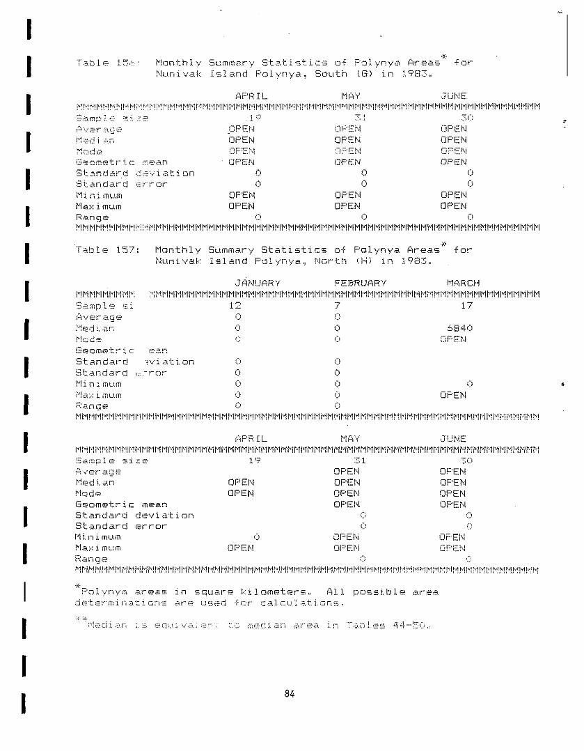
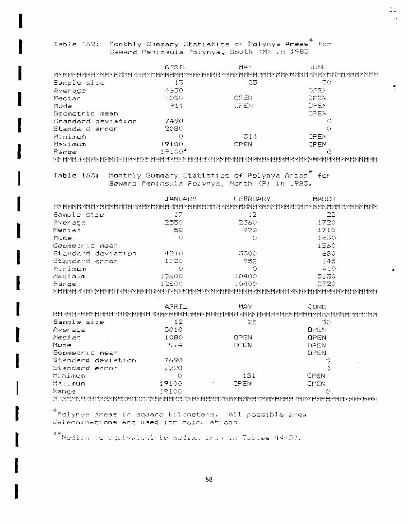
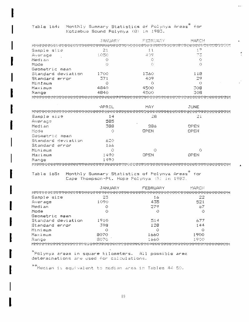
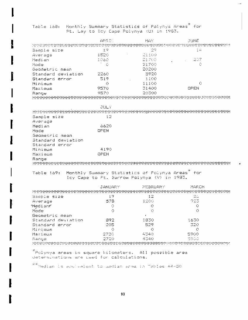
This quarter we have condensed these data into a statistical

summary (attached as Appendix 2) giving a wide range of

statistical parameters

3. Data Received

and archive daily NOAA

for each polynya on a monthly basis.

and Archived. We have continued to obtain

AVHRR satellite imagery of the OCSEAP

study areas around Alaska.

daily coverage of Alaska by

Secause of the three-to-four times

these satellites, we cannot possibly

IIIIIIIIIIIIIIIIIII

afford to purchase a COPY of each

charged. Thus we select only the

at the $10.00 per COPY rate

best images (approximately

three per day and purchase them” in positive transparency format

directly from the receiving station at Gilmore Creek). (Our

experience has shown us that positive transparencies retain the

highest information content for analysis and reproduction

purposes of all data formats other than digital tapes.)

In addition to the positive transparency format data, we

also receive hard COPY facsimile transmission positive prints

that have been used by the weather service. There is a great

quantity of these prints, as they represent at least one COPY of

each day’s image and sometimes digital enlargements and

enhancements of

weather service

Gilmore Creek.

is considerably

particular areas. These are sent.to us by the

about a month after they are transmitted from

We archive

diminished

transparency) because some

investigators may be found

these data (although the image quality

from that of the positive

feature of interest to OCSEAP

on one of these images which did not

appear On an image judged to be one of the day’s “best” images.

Following these criteria, we archived approximately 517 positive

transparencies and 3998 positive facsimile prints this quarter.

Our ‘“Quick-Look” ground station received a total of 184

images from Landsats 4 and 5. These images are often digitally

enhanced and enlarged with copies of these

well as the standard l:lM scale print. In

2

products archivad as

some instances we have

IIIIIIIIIIIIIIIIIII

obtained images at times when the sun was below the horizon - yet

ice conditions are easily observed. .This is an additional value

of our ground station and image enhancement capability.

We also continue to receive and archive the NOAA/Navy ice

charts published weekly and the drifting buoy data published

monthly by

ACTIVITIES

the Polar Ocean Centsr in Seattle.

NEXT QUARTER

1. We are anticipating providing remotely sensed data to

OCSEAP investigators performing field work aboard the NOAA Ship,

Surveyor.z

2. We will continue to collect remotely sensed AVHRR and

Landsat data.

3. We will monitor the availability of

microwave data which should become available

O c t o b e r .

4 . C o n t i n u i n g Polynya Ana

the SSMI passive

in September or

ysis. Our earlier efforts to

relate polynya size with local winds on a monthly basis did not

yield many positive correlations. In order to test whether

monthly sorting is too “coarse’” we will divide the data set into

hi-monthly sets and perform the analysis on that basis.

1 3

IIIIIIIIIIIIIIIIIII

On the other hand, we note Robert Pritchard’s recent OCSEAP-

sponsored research which reports poor correlation between ice

motion and geostrophic winds. We want to investigate these

results for their implications to polynya formation and size.

4.,

II1IIIIIIIIII1IIIII

APPENDIX 1

5

III1.IIIIIIIII1IIIII

E v e r e t t TornfeltM i n e r a l s M a n a g e m e n t9 4 9 E . 3 6 t h A v e n u eRoom 110

February 18, 1987

Service

.-

. .

Anchorage, Ak 99508-4302

D e a r M r . Tornfelt:

Enclosed with this letter are three enlargements of AVHRRimeges from September 15, 18 and 28, 19S3. We conducted a searchof imagery available since 1973 and found that this set of imagesillustrates best the conditions encountered by the whaling fleet.However, the conditions shown here may be one “cape” northward ofthe location where the fleet was caught. (See dates on back ofimages. ) The September 15/18 pair shows how fast the ice canmove shoreward. The ice remained there and can be seen “freezingin” on the 28th. ,(Notice that Elson Lagoon North of Barrow hasf r o z e n o v e r . )

.

Best regards,

Bill StringerAssociate Professor ofGeophysics

BS:jd

encl .

cc : Jawed Hameedi ,

Geophysical Institute, University of Alaska, C.T. Elvey Building,Fairbanks, Alaska 99701

PHONE: 9074747282 TELEX: 35414 GEOPH INST FBK

EsIabllsh6d bv Act of Cmgrass, ddlcated to the maintenance of vOlah”,lcal rwemrch co”eer”inn the Arctic region,.

“-

IIIIIIIII1IIIIIIII

&RzL~/._..--— --—

---- ---- ---- ---- ---

,

m

N

III

IIII1III1III1III

70° N.

080.

~60.

6 4 °

6 2 °

6 0 °

I 80. w 1700 160°

QWrangelIsland

\

\

Chukchi Sea

59D- Norton Sound K

P

/2/ Yukon

Delta

@

~ St. Matthew

[

Cape RomanzofA Island

Q~ - ~ ,

HFJ;~~n;k o 100 200 3 0 0 400KM

G o 100 200 Ml

Bering Sea

170° W leo~

Figure 1. Map showing approximate location of persistentpolynyas in the Bering Sea/ Chukchi Sea study area..

r2er4

70+

6s~

664

64°

624

60°

.

9

. . .

IIIIIIIIIIIIIIIIIII

TABLE 1

IDENTIFICATION OF POLYNYI

LOCATION OF POLYNYI

St. Matthew Island Polynya, S,outh

St. Matthew Island Polynya, North

St. Lawrence Island Polynya, South

St. Lawrence Island Polynya , North

Nunivak Island Polynya, South

Nunivak Island’ Polynya, North

CaPe Rornanzaf POIYIIYa

Yukon Delta Polynya

Norton Sound Polynya

Nome Polynya

Seward Peninsula Polynya, South

Seward Peninsula Polynya, North

Kotzebue Sound Polynya

Cape Thompson-Pt. HoPe Polynya *

Pt. Hope-Cape Lisburne Polynya

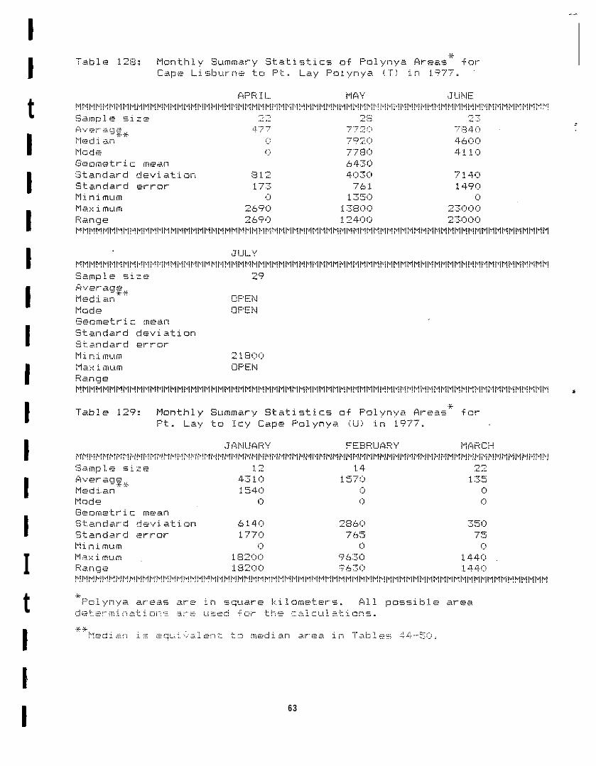
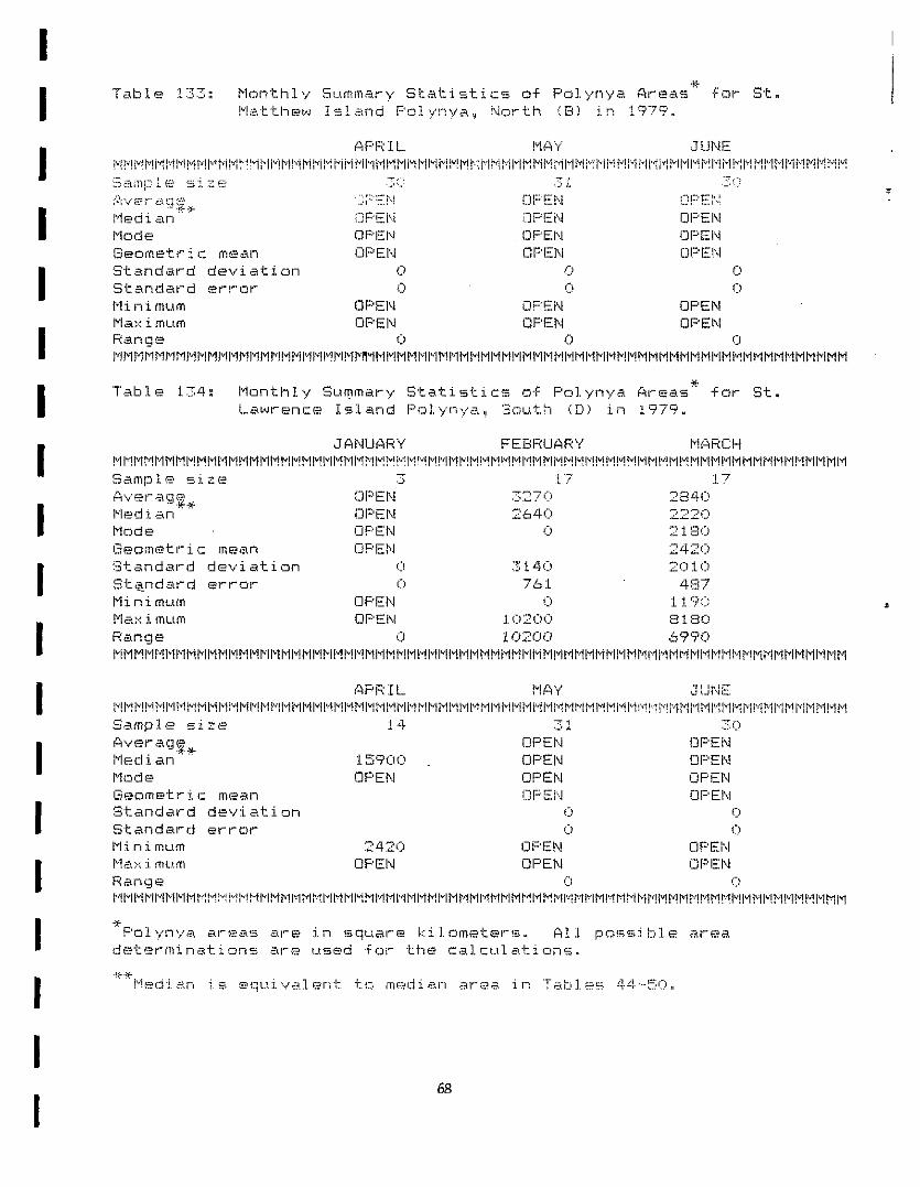
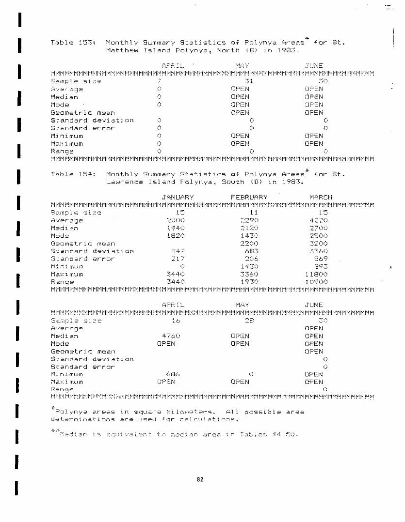
Cape Lisburne to Pt. Lay Polynya **

Pt. Lay to Icy Cape Polynya *’

Icy Cape to Pt. Barrow Polynya **

Chuk:tsk Peninsula Polynya

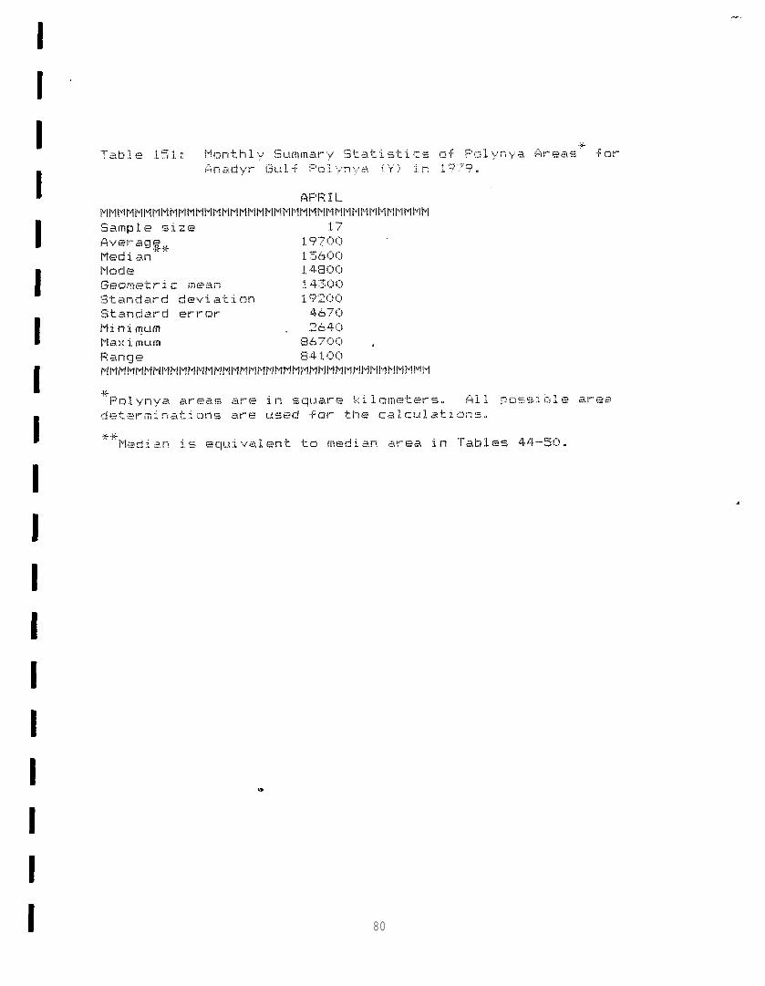
Anadyr Gulf Polynya

* Carltonr 1975** Chukchi Polynya (Stringer, 1982)

10

CODED DESIGNATIONON ALASKA BASE MAP

A

B

D

E

G

H

I

J

K

L

M

P

Q

R

s

T

u

v

w

Y

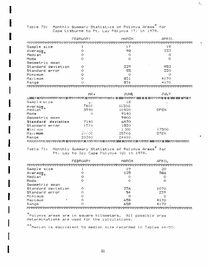
III FEBRI.JA?Y rh4Ecb] (WE I L

!qM?'lhil~PllqMlq lqMMMkl PIMllPllqFl MM PiIq Pll?l>llVllqlvl14 lqlqlqlqM!+lq Ml? PllVIVllqFll{l Yll"!t!PlhlPllvllVl14 Mlql~Mlq Pl~4MlqlVlRlYPlMlu}S a m p l e si.z~ 1. &

I14

$lveraqgri. c)lMed!L aII

S&v(-lc) 722;) z (j 4 (:1

Node 1:) i 140 UPEN

I

G e o m e t r i c mean 3660S t a n d a r d d e v i a t i o n [:) 2?00S t a n d a r d arrnr [:1 i 5?(:INinimum (:) 4 9 7 436

IIkla:: i mim [:) vii(:) CIFENRange c) E%lclMMMIW! M IM M M Pi MM 1“11”11’! !~ M M M MM lMiW”! M PI M M M IMIVIM I“!MM M MMlvlMMMMPl IM P!I”W IMM IM M M M M IV M IV! I’’II’IMIW 1+1”1 1“1 !WH’1

IIIIIIIIIII

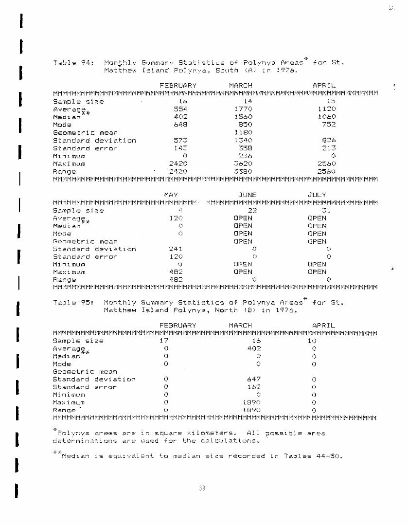
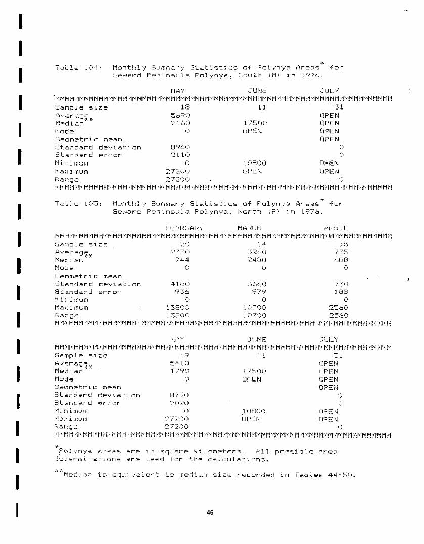
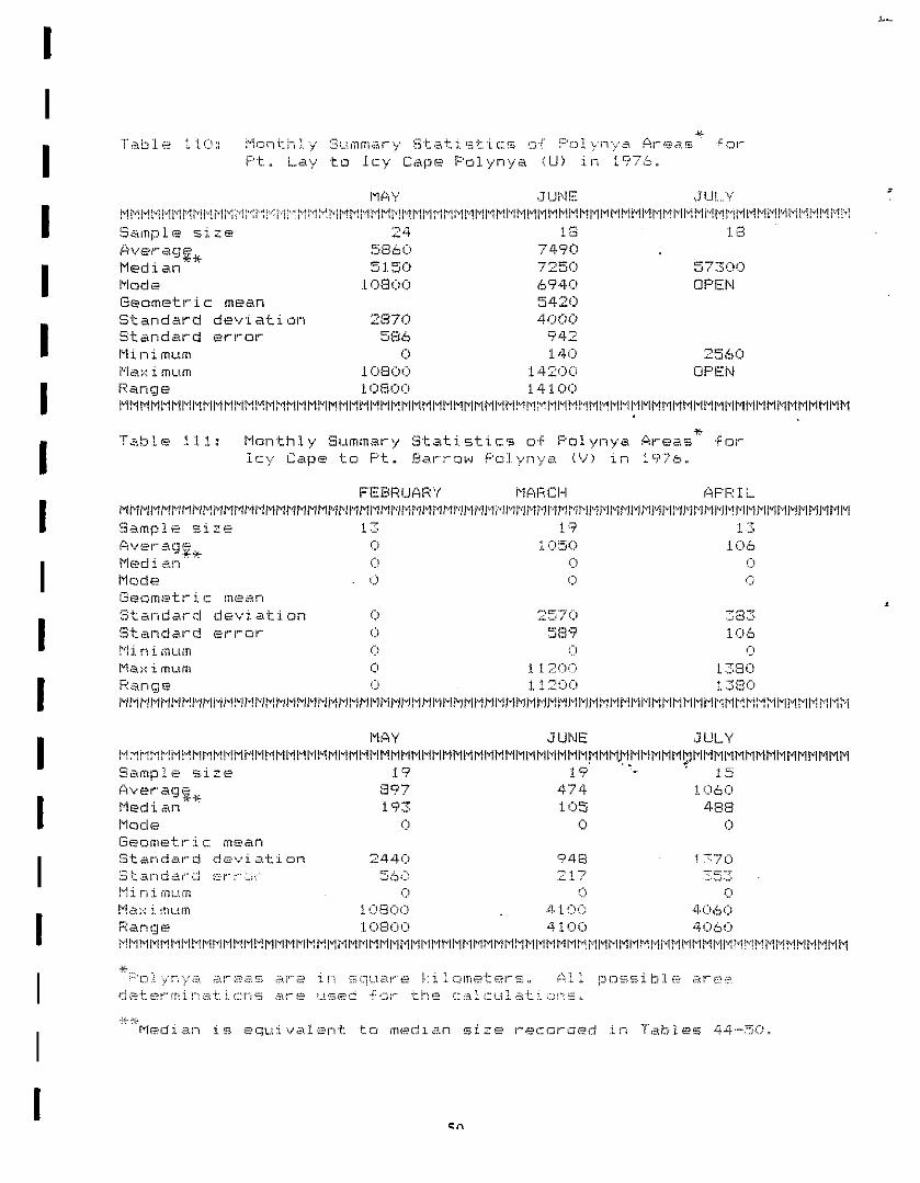
Table %: M o n t h l y Summar-y S t a t i s t i c s n+ Palynya AI-Eas*

for- St.M a t t h e w Island Polynya, lNortln ( 5 ) i n 1?74.

FEEmwr7Y Plif(cn w% I 1-

Pll+FlMMMMklPlMlVl~ilqMr~lqlYlVlFlFllqlqlqMMlqlqMlYMMlqMPlMlqPlMlqlVllVMMlqbllvlFl~0lql>lMMltiPlMlqlYllyllqlqMl4MliMMlqlqMMS a m p l e size 1 ~ 11fiver.ag~~ [:) (:)Medi an (;) (j (:)lMc)de (:) <:) [:1I?eometric meanS t a n d a r d d e v i a t i o n (:) 0Standard error (:) (:1h’li n]. mum (:) !:1Max i mum

Q{:1 ::! OPEN

Range c! ‘:.>MMlYlslFllqFlFlrll"lMMMPlMMMMlql~lvlFll4MMFlMMlWMMlAl~FlP!FllWl~l~lVi,ll~FlPll>lFlFlPlFlMMl"lPlMPlMPlMFiMPllvIt4lql+lNMtflrllq

I1 11

IIIIII1IIIIIIIIIIII

*T a b l e 55: lMonthly S u m m a r y S t a t i s t i c s a+ F’nlynya Area= for St.

!Platt hew Island Pnl. ynya, l\lnrt. h (B> i n 1974.

Table 57: Mcmthl..y Sum(nary St.a’Ei~tics Of Fal.ynya Areas * fmr StmL a w r e n c e Island I>olyn,,,a, Snuth (D) in 1.974.

MAY JUNE JULYMl~l~MMMPlPl141'ihMl~ PIPIMPIMMIVPIMl~ FlFll~MFlhlMl`lPlPlPiMPlPlMlYMMMMl~MklPlMPlPllvlPlPlPlPihiPlPlFlMl"lPlMMMMFlFlrll~Sample size 31. 3 (:1 5fiveragg+ OF’EN OPEN OPENFled i an OFEN OPEN OFENlMc)de OPEN OPEN OPENG e o m e t r i c m e a n OWN OPEN OPENS t a n d a r d d e v i a t i o n (:) (:) [:)S t a n d a r d error [:) (:) c)Plinimum OPEN OPEN Ol~EhlMaximum OFEN irFEN OFENRange c] (:) !.)F!MM 1.1 M M!~lqlgl.llq 1.1 M I.l}$llv[ lqlvIPl PI 1.1 PI ~1~11.1~.11.l 1~ l~Pllqlv! 1.1 Iq l.! Iq MM M 1.1 M M 1~11.11~1 Iv! !? l.! lvllYllq 1.1 [q M !.!Iv!MP!, M IM M MIVIMF!MP1 IMM M

12

IIIIIIIIIIIIIIIIIII

Table 5S: i%nthly Summary Statistic= Of Fol’yn?a h-=as*

F(3T st.I-ewrence I s l a n d F’ol:,nya, I\In!-th (E} i n 1974.

FEBF:U&E’t IMAF:CH WF:l Lp~!"!lY]?ql.ll.l l"ll"lp//p?llqlql") lyMlqplp[}ql.lpqlvl~q l.}rillqpqiql"ll.l \qlqpll.~pq[~ll"l lq~ql:l.~[.lpllq l"\ Mp\!q Mlq;qp!Mlql.l\"[ lq]qp[jYllqpirl rqlq Mlqpql.jl.l :Sample size 1 :1:1 9Averagg+ (:) ol~~dian” (:1 i:) [:1Mode O (:) !:)G e o m e t r i c m e a nS t a n d a r d d e v i a t i o n (> (:1standard errar o !:1lMinimum [:1 [:) !:)lMax i mum !:) !:)Ranqe

ilFEN!:) (:)

lqPllqlqFlMlYl.ilVlFll.lFll"lMMMPlFilVll"lMMl4blFlMlqMlqlqMr4FlMlVl"llVll.ll.lhlPlFlPlPllqlVlFlMFlMlqMPlPll$llYllVlFllvlPWllAMMMMMMt4M

lM13Y J(JNE JULYP! l’! 1$1F!M1!t“!I“t1~1’11’1 l’i PI M M M M M P! M M IPI PI M kl IM 1’1 1“[ Pi M M M 1“1 M P! IV! M M M M 1,1 M IN M Ivl H IPI M M M M H M M M PI M M M M lM M M M rq M M N M MSample ,Size . 1 2,(3 ~.. . . .,(averag~. OF’EN oPEN OPENlqed i am r2F EI\l iIPEl\l OPENMade OPEN OFEM UFENGemmetl-ic mean op~l~ O?EN OPEl\lS t a n d a r d deviation !:) o !:)Standard error (:1 o (:)M i n i m u m OPEN OFEN OPENMaximum OPEN OF’ENRange

o IF. E N .!.1 (:1 (:)

MPIPIMl`llVllqlqlql? MVlMMlYlqlVlMMlqPlPlMlqlqlVlMl4lqlYllvllVllqlqMlYlqFllqMl~lqMMMMl?lVlMl~MP4MPlMlql+llqMl4MMl~llqlVlVMlVlMM

Table 5 9 : Monthly S u m m a r y !5tatisti(:s of Polynya Areas * f o rNunivak Island P(nlynya,, South (E) i n 1974.

FEEIi71JAF(Y MARCU AFI?I.LMMPll'll'lMMlqrl MMI`lFlMl7l7lqM/4Pll'll"llqMlW!PlMl?PlhlMMlqP(MMMPlMMlqMMMMMl?lq!,!MFll7l?PlFir+MlV!qMl?MMMMlWMFlMlqSample size 1 ,. . +’ 9 ii6v.=ragg* <:) 372[:)lMed i an (;) 4460 414 (:10Made (:) (:) OPENGeometr ic meanS t a n d a r d d e v i a t i o n c) Z$31.C!S t a n d a r d t?rrar <:) i 27[:)Minimum C)v 10 s [:)i-iaximLlm o ~ ~ !> !;, OPENRan Ge !,, ! 9 ~ (:> !:!MMlVllYlVl"l141+ !Wl14M[lPllVlFlPll~ MPql9Mrll+l4MFllqlYPlt~lqPlFlMlql"lMlqMl,ll,llqMlqlYMMMMMMMMMFlWMFlMMMl.lMl.llyplplFlKlM

13

I1IIIIIIIIIIIIIIIII

“Tabl = 55’: lManthly S u m m a r y S t a t i s t i c s a+ Palynya Areas1+

+ orNunivak Island F’al!; nya, Scuth (G) i n 1974..

T a b l e A(:); Monthly S u m m a r y S t a t i s t i c s a+ Pnlynya Areas * forNunivak Island F’olynya,, North (1-l) in 1 ? 7 4 .

ri~y J!JN~ JULYlqlqMMMMMMMPlMMlqMMMMlYMFlFll~ll.lPlFlMlqlqPlMlqlYlVllWlMMPllYlqMlqlYPlMMFlMFlMMl~lqlY!Fll,lMlYYlMMPlMPflqPlMPlliilVPlS a m p l e size i 3 !:) 5fiveraq~a OFEN OF’EN OFENMeclj.an ““ OF’EN OFEN OPENMode OPEN OPEN OPENG e o m e t r i c mean OPEN OFEN OPENS t a n d a r d d e v i a t i o n 0 (:1S t a n d a r d error

(:1o (:> [:)

Minim,.!m OF’EN OPEN op~~j&!a.:.: i mum OPENRsr}qz

OPEN CIPEN .!.! v ,::}

!lFlFl!qlqMPlrqlYPlMh4 MPlPlMlqlqMr,ll>ll$llVllq]vlMMMPllqPll~llYMMlqPllqYllYlql3Mlllq~ll,[lqlqMMlqMMl"llq!q[~lq~lMMlqMl,[Ml!~lv[!,[/fl

*

I1IIIIIIIIIIIIIIIII

FE BRu(WY IMA17CH AP!?:[LM!~MMMlql.llq~lMMlqMFlYllYl~ll~}!~l>!hl!ll~MFll4l~lvlMI??llqly!Ml4lYl~Pllwli-!!WllqlYllqlVllY!~P~lVllY!F?l>!lq!,!l!NlqlYlq!-l!W!l~!Vl!V[lqk!lqPlM!q ,:Sample size t 15 9fi\/erag~,P (j ?72(:)M e d i a n c) 2!:)00Mode

‘54 6 (:) o0 0 OF’EN

G e o m e t r i c m e a nS t a n d a r d d e v i a t i o n (:1 14(:1 C![:)standard errar (:) z,52(jMini,mLlm (> O 329MaximLlm O 4 22(:)0 OF’ENRange (j 42 2(:)1:)lvlPlPlMl~MMlYlYMl`iHMFlMMlql4MMMMMMPllqMlVlPlPlFll`llVPllYMMMMlqMMMMlqPlMlqFlMMl'lMlqMMlqPlklMlqk}MMMMMMMFl

Sample size . 1 ~ ,::)J 5Weragg+ OF’EN OF’EN CFENIvledian OF’EN UF’El\I OPENMode OPEN op~~J OFENG e o m e t r i c m e a n OFEN OPEN i]FENStandard d e v i a t i o n (:1 [:) (jStandarcl (=rror (:) (j OlMinimL(m OFEN OPEN OPENlMa;.:imL(m OPEN C!13EiV OPEN ,Range O 0 0MMMMP!M IMMM M M IMM lMMMIYl M IV!M M IMMMMM MIM 1’1 MM 1“1 II MMMMMM M M MMMMM MMMMMM!7 IV!II M PI !7 MM FllYlqlvllVll$ll.l PIIW-1

Table 62: Mmnthly SL!mmary S t a t i s t i c s o f F’olynya Greaz * +01’

YLik13n Delta F’olynya (J) in 1974.

FE!3F:uAF:Y FifiRCH CiP!=:ILklMMPlFllVlql~llVlqlY14 l.lPll$l!4l,lMMlYMlqlqlYlvlMFiFl!,lMlYllqMlqlVlv!l4lY!4l-llqlYFlllMMlqltilqlqMMMlq!llVlPllqPlMlqPlMlqlqMlYlWl!4lVlSample 5i2e 1 14 15$lveraq~,~ f) [:) 480(:)Iqedi an (j (:I oMade U !:) (:)Geometr ic meanS t a n d a r d deviatimn (> [:) 543<:)S t a n d a r d e r r o r i:) t;) L 4(:!<:)Mi ni mLtm L) 0 (:1Max i mLlm Cl (:)!?=?llye

i 240 c)c) (:1 i 24. (:)(:>

MMlYlqMFll~lVlFlMlqMPlHP!Fllq!llYlMMMMPlPl~lMMFllqPlPlFlMPlFllVlFlMl5M!?MFlFlMlqMlfll,lFlMl,lMFlPllqlvlFlMt{lPllq!,lPlMPllqMPi

115

IIIIIIIIIIIIIIIIIIII

p,fiy .JUNE J (J!- YIM MIVW MMPI P! M ~1 M M M PIMIVIMISI MM IMM M !P’llq IMMIY 1“1 M IPI IM lP’lMMM P! M PIMM MP!M 1! pi !! Mlvl W MIWII’IMM M 1“1 M MM Pi MMISI IMIVIMMIVI M :,%~(n~’1 e si T.e t:= - .-.,:, ,,-, ~&erag~+ OFEl\l 01=, EN flPlea’ian [:) OFEN OPENMode (:) OPEN OPENGeomekri. c mean OFEN OF’EN5tandard de.viatiohr (:) (:!Si:aimdard error o [:>!Vli n i mum o OF’EN OF’EN!V[a;.: i m~~m OPEN OFEN (y~l,]Range <:) [:)!4FlMMFl!~lqlqlqMM!4 MlqMl`llY!lqlqMlqPll"lMltilvlltil"llqlqlqMl'llqPlFlMPll"lPflfilql?l`ll`lMMltilqlqM!4l"ll'llqMlqlqP!lqlqPllqMlVll'lMMMlV

i-m Y JUNE JUl_’fM~~!~,~~. i~,mP]lqM~l[q!l Ml"llqp~lql~MIY [~l~l.iYll,llql~ MlqMMl"l MM Pll"llqlq MMlqkllllVl$lFl P~l.lFllqlqlVl"l Pll~[.!}.(},ll~[ l~l~MMp~{qMP~l"] l"!Sample size i? 3 (:) .

Averag~,~ OPEN OPENdMedian :[ 7200 OFEN OPENMode OPEhl OFEN OPENGeometric mean OFEN OF’EN‘Skandard deviatimn [:) [:)S t a n d a r d =rrnrlMi n i mum

o ! .!I<) j. C)(:1 CIPEN OPEN

IM ax i mum C! PEN OPEN CIF’ENFiange o ,::?PI M lMMl”l!Wq P!MM lWll,l IV! P!rq l! IV! MI,}M IM IM MMMI”IMMMMP MM IMMMMM IM IM M MMMM MMI”IMMI”I M M MM IMMI’lMM M lMMYi FWII”!M M

16

.,

-.

IIIIII

IIIII

IIIIIIII

Table /14:n.

lPi0nt171!f S u m m a r y 5tai:i5kic5 of Fnl.yn:fd Rreas + c)l-N5me FOlynya [ 1 - ) i n :1774.

FEEIF:LJAF:Y MGRCH APRIL

M(3Y’ JUNE JULYIqPIMMMM Ml! !,!i!MMFlkIMMMlq IM HIYIvIMMPI Iq IM IXIIVI rwiww I~Mwl N m M PI tWiVIl~MHM MI*ll’tMIVIiVIl~PIPII~ IPI !PI r,!mi~!i”lwi~li~ll”ir!Sample s i z e 19 ?3 (:! ~

fivwq~+ 13 FEN OPENI“ldi an 1 72!:1 o “U?EN QFENPlods OPEN OPEhl OPENGi2ClF,~ti’-:L C (,le;, fi OPEM OFENS t a n d a r d deviatifin [:1 (:)S t a n d a r d error i-) [:)Minimum 1 (:)1 0(:1 OPEN (FENMsximum OF’EN OFEN OF’ENF:ange

,0 !.)

MM Fk’1 IMMMMMMM M N !’I!’f M1’11”1 N M MMI”II’II”IMI’I IM lYFIP1l’llqM!llql’llY MMM IMMMMMM 1“1 M Ml\lMl”!!lM M MIVIMMMMM rlMP!l~ MMFI

Table h5z Mnnthly Summar~), St ati sti c= o f Pal yny:. (%-9.+5*

F m rSewarrl Feninsu].a Pnlynya, $lou~ll (M) i n 1?74.

17

IIIIIIIIII1IIIIIIII

2:—.

Table S5: Monthl v Swnmar~/ Sl:ati sties m+ Polvn~/a Areas, * f o r

T a b l e 65: Plnnthly S1.lmmarf !3Lati5tic5 D+ F’nlyn !/s. Areas* f o rSeward P e n i n s u l a Pcl. ynya, North !F) i n 1774. ,

IPI (+ Y J IJ NE JLILYlVllYPlMMlYllyllqMPiFlPlYlPlPllqMlqMtYPlMMFlMllMlqlqMMl`llVlvlMMPlFlMPlMl`llqPlMPll"llYMl`llql'lMl`lMPll"lFirlt`ll4PlMlVlklFlFlFiMMS a m p l e <~i.ze 17 .7 i! 5Fbveraae OFEN,p,=-J i ~;”J’*

OFEN144[;) OFEN OPEN

Iblode i:) OPEN OPENG e o m e t r i c mear, OFEN OFENS t a n d a r d de,., i”ation !:) oStar, dard e r r o r [:1 (:1Mi [n i mum !.! IOFISN OFEj\lMa:: i mum [j~~N CIPEN oF’El\iRange o (:!MMM MIVIMP M M !1 Iq IMIVIMM M IPI M M IM 1“1 M FIMM M M M IM1’1 IM Pi IMIVII’}MN M IM IYIMMM IMM M I’IIVIMMM IM IVIMM1’I 1’1 M M1’ll’ll’l!y!!q M 1! N M IM M

18

.

IIIIIIIIIIII

I

IIIII1 19

.—

IIIIIIII

IIIIIIIIII

I

I“IfA\’ JUNE ,.71JLYkll"lF!VlMM}vlhllVlMr4 l>il\llv!lql+FIMMPllllV! MMMPlMlvllWlMblPll~lMltiMPllqlllqlqMMFilqMlqlql"lhll"ll"ll~[]"llq~lMKf}q!qF!FlMMMM~pl!~MSample size 3 <:) 15 ..-.f%erag~,~ 49’?U 1 I 4 i:)<:)Medi an ~’$~ 1 (:) %:!1:) ~ $lq(>()Node (:) i (:)7 !;) (:>G e o m e t r i c m e a n 6aZtjStandard de<,iatj.un 77&j 77<) oSt.al-,darcl er-r_or j, q~(, i 99(:)lMini mum (:! ~&~ 17501:1Maximum T {-) ~ (j ~:! ~ r 7 (-] ~-,..,./ . CIF’ENRange .7, -) 7 ~-),-,G . . . . . 2:54 f:>[:]M rum i~ MM ml ww M rwwrrwrm rg rirwiwl 1.1 1“1 PI lMMM M ri F41v1M IMIY r~l M IMMI+!IYI ivl MIWylMMMMM M 1P! !YI miw M i~lHlqi.1l~[r4i.iigl.1

20

,,,.. .. . .

1IIIIIIII1IIII1IIII

r~i~ Y JUl\lE JIJLV1“1 MM IM M IM MIWYIMFIMMM IM PI IM M MMPIMMM WI M MMl”llqM IP1 N PI 1“1 MMMFl M MM MIYMMM IM MM M M M MMMMM M M M MM MM M !’1 M IM,Sampl e =.1. Z(5 -/ i~Aver*9~.~e

.7,50 c1

IVI @d j. sin}. i 30 c)

5? ’7(;! I !:> .+ijt:) mi=~;.j

l>l~d~ <:1 714(:1i3e0mdric m[aan 94C!()S t a n d a r d d e v i a t i o n 7141:) 6430Standa?-d errcx- L ~ T 6:) 1 ~~!:,M i. n ~. mum

.7,-, - ~ , ;:;1 3(:)(:1 i 75!:)C)

IM a ;.: i mum _ . . . :. .:. 257 (:! o (-j 1:~:,,

Range :2 i:) z (:1 (:) ~ q 4 i:) (:) #

PI W IM IM IM IM 1“1 IM IMPIMMMMMM PI M IMMIVIPIMK IM M N lMM IMM M M M IM 1“1 MF!IY MM M MMPIM Iq M IM Iki MMM MM Mlyl lq M MM MM WWllV1l’WWPl

IIIII1IIIIIII1IIIII

.,-, .

Table 7i: Mmnthly 5ummary S t a t i s t i c s 0$ Folynya Rreas’* farFt. I-ay tm Icy Cape Polynya (U) i n ‘!77% .

22

IIII1

I

I 23

IIIBI

IIII

III1IIIII

J! W\lU(W’f FEFWIJLW+Y MfiF(CHkirnrilq~,lMrnlvll~ ~lrnrn M!lr!r,ll,llvlrlr,ti4P lF,il~r4!q!qm Plllrl!4~lrnlql ql"iplrni?Hr4!qlvr irnl!r`!hlrlrnr ~lqP'll"llql~lP~! 'il"!l~!qi"i!'!l q;4!4MH!q =S a m p l e size s ~ 4&vel-agf& [:) 584 :23 (:) c!Median o 549Mode (:)

277(:)478 277(:1

G e o m e t r i c m e a n 6(:) i .2’?3!2Stsndard d e v i a t i o n (:) 418 769Standard error !:) 1a? 384Minimum [:) ?.12 234(:)Piaxim~<m <j 1. 3?(:J 4I1ORange !:) 1 i:)8 !j 177!:)lqlqPlr4M!4MMM!~ l>lMMFllql"lr~l>lMlyll"lMPllqPllVlrllqlVlPlMMl>lMlqlql+M!4kllvlMMlqPll4l>li?lYMPllVllqlYllvlMMMPiMMlqMMMFiPllqMMl>i

T a b l e 75 : Mon’khl!/ S u m m a r y S t a t i s t i c % of F’olynya Areas*

far !3t.Matthelw Island Fnlynya, North (L+) ii-I 1975,,

JfINUAi=,’Y FEBRUAR”Y M!Wk\iMWlqPllvllv!M14 l~lqMMMl~PIMl~l>} l~MMMPllYl~l>ll~ lvll*lMIYl~lVPIMl~ MMPll~l~l+l~l~Ml~ lvll~lwl!,lPlIvllYlvlMlvll~lvlMlvlPlNMl~MMMlYl*lPlS a m p l e size 1 4 49~verag~,* (:) C) [:)Medi an (:1 (3 [:)Node (:) [:) (:1G e o m e t r i c meanS t a n d a r d dm’iatim O 0 i:!S t a n d a r d errnr ~..l 6> (:)Mi n i mum [;) (:) 0F!ax i mum ! .1 ! . .. (:)Ran(J(z !;, !. 1 i:)MPlhiMl,llsl14Pl lvlFIMMlyl}vll,l MMlylPIMIVl~Ml+l lvlly!Ml>lMPll~ll~ l~17PlMl~PlPlPl l>lPil~lMl~l~MFl PlMMrlPlFIl~r,lrl141 ~l~PlMMlvlPll~lqMFllY

24

II1I1IIIIIIII1IIIII

Tabl@ ?b: I,lonthly S u m m a r y S t a t i s t i c s of Fnl Ynya Areas * +Or St.Lawrence Island ?al.ynya, South {D) in :1975.

JANUAf?Y FEE!!? uQF:Y IMAF:CHMM IN IhiMMMIvlr!rn IY IPI M PI M Ihi PI lvkwww~ isI M M M IrI MIWVWI m M N F!FtWM PI M IPI M Nm!q M FIN M IMPI IMiq i-! iq i! M PI r~ IHMMMMMMiqIq M

Sample =izs 7 ? 14iwl-ag~+. FJ7&(:) 325(:!!hledi an .41 i c!

456(:!~37(:1 4xi(:)

Mode ~~l!:) c:) i:]Ganmetri c mean ~ ~ ~, ~:1

Si:. andard c!e... i ati m{? ?5&i:1 :4 O(:! 37,5[:)Sta!-]dard m-r(~r 7.’51 (:! ~, 2ac)Minimum 2 (:}2(:)

i OC)O(:> I.)

[Maximum 271(:)(:) ‘ sq~~> :1. 22(:)[:)Range 2!51 o<:! 855[:1 7 ~-(”) t”]. . . L .MM lMlvl M M M IVIMMMI”IM 1-1 PIIWWWVI PI M N IMIWVIIVIW14 IM NMF! PI M 1“1 1“1 !PiMIYl M 1A 1>1 M PiMIVl M H M M IMP1 IPI IVIFI r,llqr’wl lkl M PIPIMIVIIVIIVIIYIN M

.

25

IIIIIIIIIIIIIIIIIII

‘Table 73: Mnnthly S u m m a r y Statistic= 0+ Falynya +reas*

+orI\.lL!ni VS),: 151, a n d F’01 ynya, Sc, Lth {E) i n 1975,,

26

III1I1IIIIIIIIIIIII 1 27

IIIIIIIIIIIIIIIIIII

J (3 N1JRHY FEBRUARY M&F:CH!’1 M M Pl IM 1-1 M M M M IM M M IM IM M M 1“! N 1“1 1“1 M M IN M 1“1 1“1 M Pi M 1“1 M M 1“1 PI PI M H M M IM M P! M !P’1 I“i M Pi IYI M K M M M Pl ivl !H Pl Iq M M ~,! Ivl IM M M 1! M M HS.amnle size ~ 11 lb

286 949[:! !533[>C) }. c) 4 (:) 177(:1

Made (:) i] 1:)Geometr i c meanStandard d“evi atian 756 12[jOtj 725(:)St<nda.rd error 236 .5#J2(:1 :1 B 1 i;)lP!i n i mum (:1Max i mum

!.! (:!.7,-, ,-) ,j& . . . z (:)4 (:1 (:! ~ ,3 !] !:] (:)

Range q (-, [-, [-) z (:}4 [:! !:) ~ ~ ~:, ~:, f>. . . .PllTl"ll-ll"llYllqFIMM MMPIMMMIVll!PIPIPllq llMMl%ll"llfi14 PIMPillMIVVIMPi 17PilYl$lFllqMPl Ml+lFIMl}lPIPllVll,l FlFlMlYMFll?MMMMFlMMM

JAiWlf41?Y FEEIF?I..JARY MfiRCUlqRlql>ll>lP!lYIMMIVlv! lVlMlqPl!4F4~,lNlqlql.l!4lqPil~lqlglqMlqPlMPllqlql.llYllll~lMMlqlqlql7MMlqlql,llqlYllYFllqlqPil,}lqFl!qMIqMMM!4lql?:Eiample size .3 12 1. z

~“~ra~% 22 1 76.3(3 45.2C)M e d i a n (:) ~ <:) ~ !> 97(5Mode 1:) !.) C]GeOmet.1-ic meanS t a n d a r d d e v i a t i o n 625 ?68(:) 73A(:)Standard error ?? , 27?(:) :210 (:)Mi ni mum (:) ,: .) oMa;.: i (mum 1.773 so 4. c] !;1 2 !5 (:) t:! (:)F.: a l-l (j e ~77(:! 2. (:! 4 !:> c) 2 !7 (:! !:! !:!Nl`llqMPllv:PlFllYlsll>lldi<lMMlYlVMPlYlFlMNHPlF!lh!l>lP!Ml?lYPlMPlVlMlql>lMMMMMlq!{l!~!4PlFlMl"llvlMl4FlPll}il"llvll?MMMHMMMMM

28.J

IIIIIIIIIIIIIIIIIII

. .!

&i=F: I !.. 1MA% J [JN 1:PlPll~!'l!~Plf4 r4NMP`lMl~lvlYl l`ll!MNl`lr41~lvl!v! !v!rl!'!?'lt41V!~ lvll~14PlljPlllY! Pl!!rllYr4?qWlVlq l~ll'lMl"l14kll`i lYl"ll'lP'll"!Pl MM?4lqPlPllqlqM :Ekmple size ~ .1 a 3 <:),#,vel-’afg$* 165!:! (:IM e d i a n ~qq !:)Ik!d=

OPEN[:1 [:1 OF’EN

G e o m e t r i c neanS t a n d a r d de\/iation 193(:! (:)Standard error 4.22 i:)lPli n i mum (:1 C) t:)Max i mum 5760 0 OFENF:anqe 578(:) (:1MMPlklMlVlqMlgPlMl'llqMMl`ll'llvINlWlPilqlqMFlMMlvll'iMPll`lPlP!Mlqlqlvll'ilvlMMlvllY!qMMMl`ll`lMMlYMl`lMMtflNhlPll'll'lMMP!MMMH

,

29

. .

IIIIIIIIIIIIIIIIIII

Plc)de (;1 0 C!Gecrnetric meanS t a n d a r d devia.tj.on .7. . . , 9 43?(:) I 94 1:)S t a n d a r d errar 143 1 ?.5C ,514rM,i n i mLtm <:, (:) (:>Max i mum V54 987(:) 5 z (:1 c)Ranae 95.4 ?s70 6 5(:) (:)IVIMM IMN M MMMFIM M MM MMMPIMMM M PI M IVII’lMI’I 1+1 M MIW1M17 MM lPl MMIWIMMMI? lwlMr’ltik_iiW’lM M M 1’1 M Iyl IPII’IW1 I&l IMMMI’I MM

30

I,,-

1II1IIIII

IIIIIIII

31

IIIIIIIIIIIIIIIIII

ITable 8.5: M o n t h l y Summary FR:atistics m+ F’ul’:;n:/a A r e a s * fur

i.::,oi:zebu~ anund F’(z1 ynya (U) i n 1?75.

J Ah iJ fl 1? Y FEEF:!.JflR”f MiJf?CHl’! MMP!!1!4!’!!’!!’!1417 MM RMlqMP!Mlq IM M M H MMMIYIM MMM?II”I M M M iq NMPIM M M IM M!Vt’li’lMM!’’lFi M PI IM M lq MIVW!!qM lqplM IM PI I!!.!:Sc+mple size 7 ~ 11

[-’’’=’:a~s++:1 ~~(:) 137[:1 !:) .

M*d I an2ss(:1

(j i (j%)(:) :~~~(>Made o 1040 [:1 oG e o m e t r i c mean 123(M2S t a n d a r d d e v i a t i o n 177[:) 8b4~j ~ ~ ~:, ~:,

Stiandar!j error 59!> 2E8C! 755Minimum ,:.1 5(:1 1 !:) !:1IP!ax i ,11 LLffi 472(:) 361(:)() ~ ~ ~:,,:,

Range 472(:) 28 1(:!!:) 7 J[:)i:)MM MM 1’1 M M IM lVIPIMWMMM M IM PIPllvll’lMlq M M IM M I“II”IM IMP! N MMIVIIVIM PI 1“1 Pi IMMI”IMM M 1“1 M M!WWM M MIVIMMMMMIVIMM MIS! NI”(M

I 32

IIIIIIIIIIIII -“

I

IIIII

‘Table 37: I.imnthly Summary Statistics nf Foiynya Areas ‘+ forCape Thmmpsoln–Pt,, Hope PolyIIya (F:! I.!I iS75.

fWF:IL 156 ‘Y J lJl~iEWI”IF4VIIVWI IVIFIMM M M!,llvllSllV!!,l lVIPl MM IM M N M IMMI’,11”1 M M IMPIMMPI MM Iq M IVIMI”I M IM M PI MMI’,IY IY MM M 1.1 M M PI M }PIHW I,!M WW!!WISample size :L B i .5 13~verag~+. ~?75 313Median 433

:1.7 40(3(:J 343

i’locl e 1;1 !:} !:1G e o m e t r i c mean5’kandard d e v i a t i o n ~ ~~~, 37:, ~~~f)f,

Standard error 317 9Z Llz30lMi ni m u m [:) O i:)p!a).: ~ ,m~,~ 3:3 & (:1 !302 !5 (:J 5?:)(:)Range 3850 56.2 .5 (:)5 (:)[:)MM M M M M lMMlvl MWIMMM M *I M N MIWW”!YI M MM PI I“IIV! M N M 1,1 !“II”IM PIIYIP!M MM M MMP1 M Iqki IYI M !“1 M lwlpih,ttMIW! M M F’Will MMIVIMt,l

33

. .1

,

.,-.

IIIIIIIIIIIIIIIIIIII

*

34,

IIIIIIIIIIIIIIIIIII

. . .

35.,

IIIIIII

I11III[IIIII

# ;-.: ~: ~ ~ _ ,.. J I.JNEM IPI M M P! M M M M MIVI Fllvll”l 1’1 IMFI 1“1 1“1 M M 1’1 IM MM PIWP’I PI M MMM Iv!lvl k! M M MMM IWW+lI” M M II PI Pl!v!IWIM M I’!M IM !q Iq t+ !>l M MM M IVIMYI !’1

.

36

III1IIII

III1IIII1II 37

. .

IIIIIIIIII1IiI1I1II 38

II

IIIIIIII

IIII

II11I 39

..

40

III1IIIIIIII1IIIIII

IIIIIIIII1I

IIIIIIII

M&’{ ,3~JNE J 1,.L. YIV! IPI PI !! !4 i!’1 Iq IM IM IM M IM M P. M M IV! Iyi’! M 1’11’1 IM M M IN IN H 1“1 PI M !,1 M W !1 II IM !! M IM M M IM IM 1“1 N M P! IVI lsl M Pi 1-1 M 1,1 M IS! 1“1 IFl M M P! IM IM IN 1“1 l“! M M PISample size 13 -, n :3 1,Avel-<3[g ~:*. OPENI’l,adi al-(” ‘“

ilPENOPEN OPEN CPEN

Mode OFEN OPEN OF’ENG e o m e t r i c m e a n OFEN oplq\!Stan(:l.+1.rd deviatimn i:! (:)Stan&ard e r r o r (:1 1:)P?i ni men] !7 0,3 C) ~p~p~ OPENI“ia.:.; i mum OPEN m E INI?ange

OPENo c)

IY!MMNI’,l W lq!lFllqf414!lM MPlP4MMlVlll14Pl lqlqb!l~lPllqM~! /lhlMl.ll.[!414 Ml?15!41ql"lP!lq Mpl~,l!~lp!l":l"lpll~l lqlqrllqlq[.~pl]qlqlqplr,llqlqM

42

IIIII1I[IIIII1III

II 43

.-

1IIIIIIIIIIIIII1III

.

44

.

IIII1IIIIIIIIIIIIII 45

IIIIIIIIIIIIIIIIIII 46

. .

I1IIIIIIIIIIIIIIIII 47

I. . .

IIIIIIIIIIIIIIIIII 48

IIIIIIIIIIIIIIIIIII

IIIIIIIIIIIIIIIIIII .,n

II

-..

I

IIIIII

IIIII1I

IIIIIIIIIIII

.,..

52,

IIIIII

IIIIIIIIIII

II

. . .

53

I1IIIII

II

III1IIIIII 54

1

-..

IIIIIIIIIIIIIIIII

II 55

II

III

II

III

IIIIIII1I

.,..

II

56

. . .

1IIIIIIIIII

I1IIII1I

II

57

III11IIIIIII

IIIII

1I

-.. . .

Table 123: Monthly Summary Statistic!: n+ Fol:fnya Rreas* farSeward Fenirisula F’mlyr, ya, SuL(ttl (!’1! in 1977.

58

5 9

./.. .

1

I

60

IIIIIIIIIII1.

IIII1II 62

.-

1ItItIIIIII1IIItI}I 63

11IIIIII1IIIIIIIIII

. . .

.

64

III11IIIIIIIIIIIIII

*

65

I-..

III11IIIIIIIIIIII

M .-.:* z,b ..- ,:.:’ !> w E NSeam fakri c meanS t a n d a r d clev]. ation (;) :1 (:)& (:),Stz, nciai-d errnr (;! 4(:)3Hi n i. mum ,: [:) i 7i3(:1Ma}.: i mur, [;) 267(:] W’El\lEange (:1 2,59(:!MM!P!NldMM1“11“1 PI !Vl IN PI t“! M Pi M IP1 M M M Ibi PI M H M !s1 IN M ?’! PI Iwl M Ivi F! PI IM !A! M N M Pl 17 1P! Iv! !“1 PI i-l IPI !hl t’! P! !? !Vi F PI PI PI IM p! W IM !“1 ?! !-! PI lpi PI M N

66

-.

IIII1IIIIIIIIIIIIII

1

I

67

III1II1IIIIIIIIIIIII

68

. .

I

IIIII1IIIIIIIII

I69

IIIIIII[IIIIIIIIIII 70

IIIII1IIIIII

IIIIIII 71

IIrI1II

IIIIIIIIIII1 72

-

I

I1IIIIIIII

II

IIIIIIII

s

. . .

IIIIII

I

I

IIIIIIIIIII

s

74

II1IIIII1IIII1IIIII

.

75

1IIIIIIIIIII1II

IIII 76

,.. ... “ I

1IIIII1IIII1III11II

320450 ilFE.l\l

573(:)

-.

IIIIIIIIIIIIItIIIII

-.. .

II

78

IIIIII1IIIIIIIIIIII I 7Q

I1’IIIIIIIIIIIIIIIII

—.

.

.

80

II1IIII11IIIIIIII1II 81

IIIIIIIIIIIIIIIIIII

82

IIII1II[IIIIIIIIIII

j;..

.

83

IIIIIIIIIIIIIIIIIII

,;.

IIIIIIIIIIIIIII

IIII 85

IIIIIIIIIIIIIIII

II

I 86

. .

IIIII1IIIIIIIIIIII

I87

IIIIIIIIIIIIIIIIIII

88

..,.

IIIIII1IIIIII

III1II

89

IIIIIIIII1IIIIIIIII

90

. . .

1II1II1IIIIIIIIIIII

91

. .

IIIIIII1I1IIII

III1I

92

II]I1II

IIIIIII

IIIII

,.

.

93

IIIIIIIIIIIIIIIIIII

94

I1II1tIIIII1IIIIIII

95

.

*-. ., ,, /:. ?/:.. /, ,

.-

F?UL3 ‘REMOTE SENSING DATA AC UllITION

ANALYSIS AND ARC& .

by

Williaq J. StringerGeophysical Inwtqte

Uqiverwy of Alaska-FaubanksFauixnks, Alaska 99775-0800

Submitted to

National Oceanic & Atmospheric A@ninistrationOcean Assessments Dwlslon

Mpa~k~o:flj~

Anchorage, Alaska 99513

. . . . . . . . .

. .

SEVENTH QUARTERLY REPORTJuly 1, 1987- September 30, 1987

OCSEAP Research Unit 663Contract #50ABNC 600041

ACTIVITES THIS QUARTER

1. Assistance to OCSEAP Investigators. Walter Johnson, Sathy Naidu and Jii

Raymund (RLJ 690) conducted a cruise aboard the Surveyor in the Chukchi Sea between

\-

DIYOW40September 17 and October 8. This RU provided support to that effort by monitoring .—

NOAA AVHRR satellite images as they became available during this time and producing

high quality photogmphic prints of the scenes which maybe of value to their study. It is

anticipated that some of these images will be analyzed digitally in the future to show

patterns of temperature distribution and suspended sediment in the region just north of

Bering Strait. A high-resolution SPOT image was also acquired showing suspended

sediment in the vicinity of Kotzebue.

{

At one poinL when the surveyor was located at 670N, 168012’W, we contacted

the field party to give a verbal description of the Chukchi temperature regime as d

bkinterpreted from NOAA thermal band imagety.

QsAW?!

2. PoIynya Analysk. Having completed our preliminary statistical analysis of

polynyas, we am now beginning an attempt to correlate polynya size with extemrd

factors, principally wind and temperature. We think that it would also be useful to be

able to look for correlations with currents. This would seem to be particularly important

in light of Dr. Robert Prichmd’s recent work performed for the Minerals Management

Service and reported at the recent conference on Port amd Ocean Engineering under

Arctic Conditions held in Fairbanks. On the basis of buoy position and current (relative

to the buoys), Prichard concludes that often currents are the major influence in ice

motion. We hope to be able to report some preliminary findings of this work at the

upcoming Information Transfer Meedng to be held in Anchorage during November.

3. Reports and Papers Provided. During this quarter we provided Drde Kinney

of MMS with ‘Width and Persistence of the Chukchi Polyrty&” and “Statistical/W!. XXL?

Description of the Snmmerdme Ice Edge in the Chukchi Sea.” Mr. Dick Ragle wanted

information regarding ice conditions and related hazards in Stephenson Sound and

Prudhoe Bay. It transpired rhat he already had most of our reports but did not have

“Summerdrne Ice Concermation in the Ha&on and Ptudhoe Bay Vicinities of the

Beauforr Sea.” This seemed to be the kind of irtfotmation he needed so it was sent to

him.

4. Data Acquired this Quarter. We have continued to obtain and archive daily

NOAA AVHRR satellite imagery of the OCSEAP study areas around Alaska. Because

of the three-to-four ties daily coverage of Alaska by these satellites, we cannot possibly

afford to purchase a copy of each at the $10.00 per copy rate charged. Thus we select

only the best images (approximately three per day and purchase them in positive ~ AtiHtQ O%

transparency format directly from the receiving station at Gtiore Creek). (Our P& G4

experience has shown us that positive transparencies retain the highest information 4!

content for analysis and reproduction purposes of all data formats other than di@d *

tapes.) ‘Zv

/

h addition to the positive uartsparency format dam we also receive hardcopy

facsimile transmission positive prints that have been used by the weather service. There

is a great quantity of these prints, as they represent at least one copy of each day’s image

and sometimes digital enlargements and enhancements of particukw areas. These are sent

to us by the weather service about a month after they are transmitted tlom Gilmore

,.

Creek. We archive these data (although the image quality is considerably diminished

from that of the positive traospmency) because some feature of interest to OCSEAP

investigators may be found on one of these images which did not appew on an image

judged to be one of the day’s best images. Following these criteria we archived

approximately 555 positive transparencies this quanter.

Our “Quick-Look” ground station received a total of 37 images from Larrdsats 4

and 5. These images are often digitally enhanced and enlarged with copies of these

products archived as well as the standard 1: lM scale print. In some instances we have

obtained images at times when the sun was below the horizon - yet ice conditions are

easily observed. lltis is an additional vahre of our ground station and image

enhancement capability.

We also continue to receive and wchive the NOAA/Navy ice charts published

weekly and the drifting buoy data published monthly by the Polar Ocean Center in

Seattle.

ACTMTIES NEXT QUARTER

1. We arc anticipating taking part in the upcoming Information Transfer Meeting

and Information Up&te Meeting in Anchorage, November 17-20.

2. We will continue to collect remotely sensed AVHRR and LandSat imagery.

3. We will continue to watch for the availabtity of SSMI passive microwave data

which should become available shortly.

.!

,..

4. We will continue our polytrya analysis attempdng to relate polynya size with

meteorological conditions.

FUNDS EXPENDED

As of September 30,1987, we have expended $169,372.83 of a total authorized

budget of $205,799.00.

REQUEST FOR PERMISSION TO PUBLISH-.. .,

Attached is a preprint of “Surnrnerdme distribution of floe sizes in the western ~

Beaufort Sea; which was prepared under this conuact. We seek permission to submit it +——————

to the Journal of Geophysical Research. 7-J

!.

D R A F T

SDMMRRTIMS DISTRIBUTION OF FLOE SIZESIN THE WESTERN NEARSHORE BRAUFORT SEA

by

William J. StringerGeophysical Ins t ituteUniversity of Alaska

Fairbanka, Alaska 99775-0800

Submitted to

Journal of Geophysical Research

December 1987

--

ABSTRACT

The areal extent of ice floes has been measured from Landsat

imagery of the summertime Beaufort Sea, spanning the five months between

break-up and freeze-up. In general, the distribution of floe size areas

was found to obey a power law: N(S) = NISA, where the counted number of

floes per unit floe size interval, N(S), is related to the number of

floes in the particular distribution at unit floe size (Nl) , the. floe

size (S), and 1, a parameter found here to range between -1.33 and

-2.06. The value of A decreased from -1.33 in May to -2.06 in August

and then increased to nearly -1.47 in September. An exponential

relationship with A was found among the values of N1 from the various

-15. 14adistributions: N1 = Noe . This relationship appears to hold

regardless of the seasonal variation of A. Thus, floe size

distributions were found to obey N (S) = NO (e-15” 4S)’, with a value No =

1.23 x 10-6, where No is tha projected number of floee per unit floe

size at unit floe size for A = O.

Although not observed, a value of A = -1 was found by theoretical

considerations to produce a floe size distribution in which the apparent

distribution of floe size is the same regardless of the scale at which

it is viewed. Based on the observed variation of A with season, it is

hypothesized that such a distribution might appear earlier in the year

than the observing period reported here. A value of

observed, would describe a floe field where all floe

equal numbers.

k = O, also not

sizee are found in

.‘ .

.

INTRODUCTION

The Beaufort Sea shear zone (see Figure 1) is a region of dynamic

ice activity resulting from interaction between the static shorefast ice

zone and the pack ice of the Arctic Ocean gyre. During winter and early

spring the ice in this region is subjected to recurring large-scale

stresses brought on largely by synoptic weather systems. During these

events, the pack ice is both fractured and ridged. However, the

fracturing at this time is largely limited to the creation of floes

whose characteristic dimensions range between a few tens to hundreds of

km. AS long as temperatures remain sufficiently below freezing, the

leads between floes freeze quickly to such a thickness and strength that

by the time of the next synoptic event an entirely new fracture pattern

is created--in terms of the new fracture pattern, the ice has

“forgotten” the previous fracturing.

Once tha

formed during

freezing rate is diminished to the point that fractures

one dynamic event remain very weak at tha time of the next

event, successive events will then continue to fracture the ice into

smaller flees. Soon after that internal stresses are joined by other

mechanisms of new floe formation; contact forces between floes in

collision have been observed to cause floe division (Sackinger, 1985)

and as fetches develop, waves also cause fracturing of floes (Wadhams

and Squire, 1980).

,!

Not only are there several mechanisms which can result in

fracturing of flees, but in this region, the pack ice strength is very

seldom uniform: there are partially frozen leads, rubble piles,

pressure ridges, shear ridges and even fractures in otherwise unbroken

floes resulting from asymmetric loading due to ice piled around edges

(see Figure 2). Thus as the pack ice region begins breaking up, there

are innumerable areae of relative strength and weakness in the ice field

which can respond to applied forces. Hence, in the absence of simple

applied stresses and unifOrm ice strength, One might anticipate that the

creation of floes would result in a somewhat random size distribution

but that in general, the sizes would become smaller with time.

There are various reasons to examine floe size distributions.

Wadhams and Squire (1980) , and Dean (1966), for instance, heve

investigated the relationship between floe size and wave attenuation.

The study reported here was originally prompted by a hypothetical

assessment of the release rate of spilled petroleum which had been

entrained in ice following the spill.

ANALYSIS

Landsat imagery has been available since 1972. ~hese ~ata have , ~-

pixel area of 4.8 x 103m so that flees on the order of 104 m should be by

measurable. The optimum approach to a study of floe size distributions ~w9sfiT,{

and their change over time would be to sample the size dis tribut ion of~Q *

the same ice field as it changes. There are saveral operational“w”.—

-.

“ . .

difficulties encountered trying to accomplish this ideal experiment:

Landsat coverage at this latitude has usually been only four successive

days every two weeks (although there was a brief period with two

satellites operating one week apart) . However, cloudiness and

operational interruptions make the data set much less regular than even

this schedule would suggest. Furthermore, unless coverage is

continuous, it is difficult to follow a particular ice field as it

deforms due to currents and wind drift. Thus, unless one has the

advantage of fortuitous circumstances, generally, the best that can be

done is a sampling of data from the same region over a range of times.

In this study we analyzed floe size data from 18 images of the western

nearshore Beaufort Sea which yielded samples between May and September,

1972 through 1981. From these images 26 study areas were selected, each

20X20 km.

Photographic enlargements of these study areaa were made to

1:50,000 scale and floe areas were measured by means of a digitizing

table linked with a computer. Actual areas were computed as a cursor

was manually directed around each floe on the enlargement. Each floe

waa numbered for identification purposas and a computer-generated

drawing of each floe scaled was created for verification purposes

(Figure 3). Floe sizes down to the order to 103 m2 were measured

line

but

the population of sizes less than 104 m2 were not considered valid for

analysis. However, in the example which follows, theee data are

plotted.

. .,!

. .

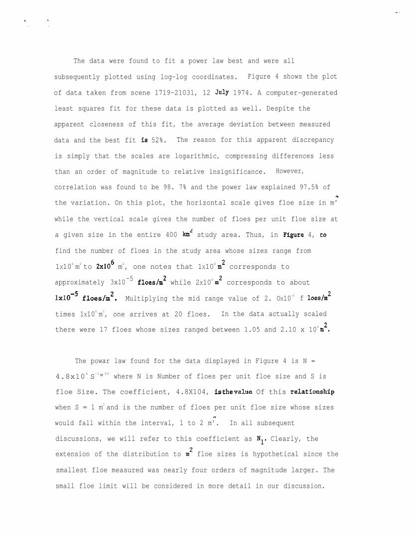
The data were found to fit a power law best and were all

subsequently plotted using log-log coordinates. Figure 4 shows the plot

of data taken from scene 1719-21031, 12 July 1974. A computer-generated

least squares fit for

apparent closeness of

data and the best fit

these data is plotted as well. Despite the

this fit, the average deviation between measured

iS 52%. The reason for this apparent discrepancy

is simply that the scales are logarithmic, compressing differences less

than an order of magnitude to relative insignificance. However,

correlation was found to be 98. 7% and the power law explained 97.5% of.

the variation. On this plot, the horizontal scale gives floe size in m’

while the vertical scale gives the number of floes per unit floe size at

a given size in the entire 400 Icmz study area. Thus, in Fi~re 4, co

find the number of floes in the study area whose sizes range from

1X106 m2 to 2X106 m2, one notes that 1X106 m2 corresponds to

-5approximately 3x10 floes/m2 while 2X106 mz corresponds to about

lXIO-5 f10esim2. Multiplying the mid range value of 2. OX10-5 f 10esfm2

times 1X106 m2, one arrives at 20 floes. In the data actually scaled

there were 17 floes whose sizes ranged between 1.05 and 2.10 x 106 mz.

The powar law found for the data displayed in Figure 4 is N =

4.8x10 4 S-1”53 where N is Number of floes per unit floe size and S is

floe Size. The coefficient, 4.8X104, is the value Of this relatiOnshie

when S = 1 m2 and is the number of floes per unit floe size whose sizes.

would fall within the interval, 1 to 2 m’. In all subsequent

discussions, we will refer to this coefficient as N1. Clearly, the

extension of the distribution to mz floe sizes is hypothetical since the

smallest floe measured was nearly four orders of magnitude larger. The

small floe limit will be considered in more detail in our discussion.

.

,,. .

RESULTS

Table 1 lists the datea, Landsat scene identification numbers,

power law relationship, percent of variation explained arid correlation

coefficient for all study areas analyzed. All study areas were 20x20 km

in size. In the cases where two study areas were located on one Landsat

image, a suffix A, or B is found after the date.

Power law relationships were found to be valid for all data sets.

However, examination of the Durbin-Watson statistics indicates that a

small cyclical variation of residuals remained. Aa can be seen from

Table 1, the smalleat correlation coefficient was .985. The value of A

ranged from -1.33 for 19 May 1974 to -2.06 for 5 August 1981, and N1

ranged from 2.99

August 1981. In

of the power and

x 103 floes on 2 May 1978 to 1.20x108 floes for 5

general one would expect that both the abaolute value

the value of N1 would increaae as a floe field is

broken up and more, smaller floes are generated. However, N1 is also

related to the fraction of the study area taken up by floes: consider

two assemblages of floes in two equal study areas, each with the same

distribution power but one with half as many floes as the other. The

value of N for the first assembly would be half that of the other.1

This study utilized study areaa where the flees were reasonably compact

yet sufficiently distinct to be identified and measured. Following

this, using the summed floe area, N ~ was normalized to a perfectly

compact condition. If the data are normalized for compactness, N1 is

directly related to the distribution!s power. This is because by

. .,.

compactness normalization we specify that the total floe area is

conserved. Then for every power there is a unique value of N1. The

values of Nl listed in Table 1 reflect this normalization. Figure 5

illustrates the relationship between N1 and 1, A semi-log plot was

chosen for display purposes because the N 1values gave a linear fit in

this representation. Thus the N1 values can be expreesed as an

exponential law: N1(A) = NOe-15. 14A where No = 1.37 X10-6 is the value

of N for the power law distribution, A = O.1

The correlation

coefficient for this exponential fit was 99. 5%.

Returning to Table 1, it can be seen even at a glance, that these

data appear to he ordered in terms of date versus A. Taking advantage

of the five date groupings that occur in the data set, we obtain the

relationship between power law exponent A, and date shown in Figure 6.

The bars on this plot represent one etandard deviation variance. This

figure clearly shows a trend toward a higher negative power as summer

progresses, followed by a sharp decline in mid to late September. It

was thought that perhaps the relationship between N1 and 1 might be

different for the September data when A was increasing in value again.

These data were plotted aa squares on Figure 5 rather than dots, as are

all other data. It can easily be seen that the September data are not

distinguished in this regard.

,.. .

DISCUSSION

The summertime floe size data fit a power law distribution over a

ranga of several decades of floe sizes. From Figure 6 we see that the

average power of this law changea from -1.34 to -1.80 between late May

and early August. Examination of the actual floe counts shows that size

of the largeat floes in the distributions chsnged from the 107-108 mz

range to tha 106-107 m2 range over this period. At the same time N (S)=

N(104), the number of floes at size 104 mz, changed f rOm a few tO tha

50-100 range. Clearly this is an indication of a process where many

small floee are being created but large floes are not entirely

eliminated. This suggests a probabilistic process whare, in each unit

of time, a given floe has a probability less than unity of undergoing a

division. As a result, aa smaller flees are created, large flees retain

some chance for survival. An alternative to this, a mechaniam under

which every floe divided, say, by half during each unit of time, would

produce a apiked distribution that grew exponentially in total nnmber as

its locus moved to smaller floe sizes. If a probabilistic process is

taking place, then the change in the exponent of the power law over time

reflects the process of random floe splitting aa the summer season

progresses. The decreaae of the exponent in late September would result

from the combining of floes as freezing temperatures reappear.

It ia interesting to consider some of the implications imposed by

convergence of the integral of a power law floe size distribution.

Clearly the aggregate of the floe sizes cannot exceed the size of the

. .. .

study area. To investigate the implications of this boundary condition

we note that starting with

N(S) = NISA

as the form of the floe size distribution,

SN(S) = NISA+l

is the number of flees whose sizes fall within one unit range of S, and

if N1 is normalized as if the study area A were completely covered with

floes,

s smax max

A = N1 f SA+lds = ‘1 #+2

s (1+2) smin min

unless A = -2, then

smax

s, max

A = f S-ids = N1 ln= Ismin

smin

gives the aggregate size of floes in the distribution whose sizes range

from Sma to Smin.

. .,)

. .

These integrals converge

1) i > -2. This applies to

under the following conditions:

all observed cases save one. In this casa

the integral will converge even for a lower size limit of S - 0.min

Thus for this form the size of the floes decreases sufficiently

faater than their numbers increase with the result that the

aggregate area of floes

i.e. smalI floes do not

smaller than any specified size is bounded,

catastrophically fill the study area.

However, the maximum floe size is bounded through convergence

of the integral and therefore must be specified. Taking aa an

example the idealized form for the distribution of 12 July, 1974

(Figure 4) , for a study area A = 4X108 m2, we have Smz =

~ ~x107 m2. This agrees well with the largest floe actually

7 2obeerved in this particular sample whose siza was 1.51 x 10 m .

(Note that this floe occupies about 1/25 the study area. )

Actually, since we have normalized the distribution to a totally

compact condition, one would expect the largest floe to be somewhat

larger than the largest floe actually observed becauae a compact

distribution would contain more floes of all sizes and a greater

chance of a larger largest floe.

It is instructive to consider the contribution to this

integral from all floes smaller than thoee which we can effectively

4 2meaeure and count, 10 m . Solving for this area yields

approximately 11J7 m2, or 1/40 the total study area. Similarly, the

aggregate Of all floes whoee sizes would be leaa than I m2 is

!.

. .

. . .

5 2approximately 10 m or one four thousandth the a tudy area.

Therefore, assuming there are no floes less than 1 mz has very

little effect on the size of the largest permissible floe in the

distribution. Even asauming there are no floes smaller than those

we ~ould measure, ~04 ~2 only incraaaes the size of the largest

floe in the distribution by 2. 5%.

Hence, application of convergence criteria to determine a

largest floe size in an idealized distribution yields a realistic

result even assuming that the population of floes in the

distribution does not extend below those sizes which we can

actually observe.

2) A < -2. This applies to only one observed caae. In this case the

integral will converge for any value of maximum floe size,

including infinity, but not for arbitrarily small values for the

minimum floe size. One way to visualize a floe field which allowa

arbitrarily large floes in the distribution yet whose integral

converges for arbitrarily large floe size, is to imagine viewing a

limited portion of an infinite floe field having such a

distribution; if one views successively larger portions of the floe

field, successively larger floes will come into view. However, the

area observed ia always larger than the largest floe in view.

In this case, the lower size limit must be examined; its value

cannot be arbitrarily small. Figure 3 shows the floe field for

which 1 = -2.06.

. .

In order to demonstrate the relative insensitivity of the size.

of the smallest floe to the specification of the size of the

largest floe, the following comparative calculation was made:

allowing the largest floe to be of infinite size results in a

smallest floe of 0.91 m2 while making the largest floe 10 m2

results in a smallest floe of 0.32 m2. Therefore the smallest floe

will range between these two values for all realistic values of

maximum floe size. (The actual largest floe observed in this

distribution was approximately 4 x 106m2). On the other hand, the

total number of floes in the distribution is far from insensitive

to maximum floe size in this particular example because the

smallest floe size is in the vicinity of 1 mz and N1, the number of

floes of unit floe size is 1.2 x 108. In other words, one can

expect that many floes in the interval between floe sizes of 1 m2

and 2 mz. In the actual case the compactneaa of the distribution

was 11% so that

be around 1.1 x

the actual number of floes of unit floe size would.

1o’.

This number haa implications which require investigation.

By the power law model used here, one quarter of the area covered

with ice was covered with floes in the range between one and two

meters square. This seems to account for an alarming fraction of

the ice covered area. However, it must be pointed out that the

number of floes per unit floe size falls off slightly faster than

S-2, which decreases quite rapidly. Hence the contribution to

total ice covered area by small floes is not quite the problem it

might appear at first. Another problem is related to the

difference between the actual observed floe field and the

. .. .

idealized floe field represented by

value of N1 was obtained by summing

the power law. The normalized

the obsened floes and

adjusting the observed value of N1 accordingly. In this case, the

normalization factor was approximately 9. Clearly, however, no

floes of unit floe size were included in this sum. As a result,

the power law does not totally represent the distribution becauae

it requires floes outaide the observable range for convergence of

the integral to the observed total

distribution has more floe area in

than the power law representation.

ice area. The actual

the observable range (> 104m2)

However, in actuality the floe

size distributions observed are noisy - particularly at the large

size end where small numbers of floes in each size category are.

found. One extra floe in the 10 km’ range would have the same area

as all the floes in the 1-2 m2 range in the power law distribution.

For this reaaon the small floe size limit of this distribution

should not be taken as physically very meaningful in terms of

numbers of floes because it is too sensitive to the variations in

the total area covered by floes. However, its computation can

yield an indication as to how completely the modeled power law

represents

numbers of

result the

the actual floe distribution. In this case, vast

small floes were not required for convergence and as a

power law represents the actual distribution reasonably

well. Om the other hand, the model representation should have had

more floe area in the observable range. One would be tempted to

change this by modifying k or N ~. However, those parameters were

calculated from a best fit to the observable

was explained to a high degree of precision.

quantity of ice placed in the non-observable

data and the variation

Therefore, the

category by the model

. .. .

should .be regarded as a measure of the “noisiness” of the actual

flow size distribution compared to the power law model.

The above argument should not be taken to mean that one should

not expect floes in the actual distribution below the observation

threshold. In this case, we were comparing the total area of flows

in the observable range of the power law model with the tntal area

of floes observed. . Nhen A > -2, there is nothing to limit the

extension of tbe distribution to very small floe sizes. The

integral will still converge and the area covered by small floes

will be finite. This is not true when A < -2. Allowing the

distribution to continue to very small floe sizes would

catastrophically overfill the study area with slush ice -

regardlaas of the compactness of the distribution. The ocean in

figure 3 is not filled with ice and therefore the actual

distribution must be truncated at some point. (In any case, the power

law would have to end at the molecular diameter of water. ) Nhen one

observes a flea field in late summer, one does not see graat quantities

of floes smaller than a few meters in dimension. There are at least two

mechanisms which would account for this: 1) small floes contain fewer

flawa sufficiently weak to result in fractures from asymmetrical loading

due to waves and collisions; 2) as flees become small, their removal

rate dua to melting increaees.

3) A = -2. ‘llhia is a special case where tbe integral is satisfied by

the function N1ln(S) . Clearly this case represents the transition

between the other two casee. This integral will not converge for

either s =Oorsma =-, so that both limits must be specified.min

.... .. .

G9

The foregoing discussion can be summarized aa follows. In general,

assuming that one knows the actual total area of all floes under the

convergence criteria discussed, for a specified smallest floe (even

arbitrarily small) and constant total floe area, the maximum floe size

specified by the distribution becomes larger aa A approaches -2 from

smaller negative values (i. e. , A > -2). When A < -2, the largest

permitted floe size is unlimited but the smallest floe size must be

specified, and aa A decreasea from -2, the size of the smallest floe

specified through convergence increasea (again, holding the total area

of floes constant). However, if in the former case (A > -2), one

truncates the distribution at some small but finite size rather than

allowing the size distribution to continue to arbitrarily small valuea,

a larger maximum floe size is required. In the latter caae (A < -2), if

a cut-off to large floe sizas ia imposed, than the smallest floe size

must be decreased. On the other hand, if one knows the total floe area

within a specified size range and has a measure of the largest floe

within a particular distribution, the model distribution can be

examined with cons iderably more detail.

If we asaume that the floe size distribution is generated by the

sequential disintegration of a few larger floes to many small onea,

transient effects would be most noticeable if the initial fracturing

resulted in just a few large floes which then begin the sequential

disintegration process. On the other hand, transient effects would be

least noticeable if the original distribution of floes in the study arsa

. . .. .. .

just after

transients

the actual

the time of first fracturing approximated a power law. Since.

arising from initial conditions are not readily apparent in

distributions, this appears likely. In that caae we would

expect to find in early stages of the process the distribution of sizes

described by large values of A with large values of maximum floe size

and relatively large values of minimum floe size.

Next, it is instructive to consider a special case, the

distribution characterized by A = -.1. In this distribution the

aggregate area of all floes Of size s~ i s

-1‘kNlsk

= N1

Thus the area of floes at each unit floe size is constant and equal to

‘1’ and the total area of floes is

smax

A = N1 f dS = N1(Smax - Smin).

smin

If the minimum floe size is allowed to be zero, then

A = ‘1 ‘mix

and N1’

the number of floes at unit floe size, can be determined by

dividing total area of floes by the maximum floe size.

. .. .

However, this distribution has an even more interesting property:

consider viewing a general floe distribution at some particular scale.

The population of floes in the field of view will have the came size

distribution exponent regardless of the extent of the flow field viewed.

However, a change of scale (for instance, by changing viewing altitude

or by changing a photographic enlargement factor) should, in general,

change the size distribution’s power by changing the distribution of

apparent sizes. (By apparent size we mean either the solid angle

subtended by a floe when viewed by an observer at some altitude above

the ice pack, or by the image area of the floe on a photographic print

rather than the floe’s scaled size which, of course, remains constant. )

while generally true, this change of distribution exponent with scale

does not occur for the distribution power i = -1.

Consider a distribution in

M and the number of floes whose

which the number of floes of area s~ is

areas are lIK Sm is P:

N(Sm) = M

N(K-lSm) = P

We now enlarge this distribution by a factor K (i. e., a linear

%enlargement factor of K ) so that floes which were originally of size

P now have an area M. The total number of floes has not changed;

however, the floes formerly of size class l/K Sm are now of size clase

Sm and have correspondingly brought their population magnitude, P, along

with them. However, the actual solid angle viewing area must be kept

constant and as a result, we now only count floes which formerly

. .

.-. .

.

-1inhabited an area of K of the total area. If the distribution is invariant under

change of scale, then the number of floes of size Sm remaina constant:

N(Sm) = M = K-lP, = K-l [N(K-15m) 1.

If we now aaaume a power law form, N(S) s S6, we can generalize the

above requirement by noting that under this form

N(K-lS) = [K-1S]6

and hence

J3 = K-l[K-1516

which is only satisfied when 6 = -1. The result can be explained in a

less rigorous way by noting that since the aggregate area of floes at

each unit floe size is constant under this power law, their number is

inversely proportional to their size, henca the incraase in numbers of

floes of a particular size cauaed by the enlargement of a greater number

of smallar floes to the larger size is exactly cancelled by the

requirement to keep the counting area

constsnt) .

An assambly of floes having this

regardless of the altitude from which

constant (or viewing solid angle

distribution would

it was viewed. No

appear similar

floe assemblies

were measured here having this dis trihut ion. Yet it does not appear

unreasonable that such distributions may exist. Based on extrapolation

of tha curve of power law vs. date (Figure 6) one might expect to see

,.. .

such a distribution in the region studied in April or March. Such a

distribution would appear generally the same regardless of the altitude

from which it was viewed. This author has experienced this phenomenon

when flying over the Beaufort

winter at night when only the

distinguishing details can be

Another interesting case

N(S) = N1

Sea and adjacent Arctic Ocean pack ice in

outline of floes and no other

seen in the moonlight.

is A. = O. In this case,

for all values of S and the number of floes at each unit floe size is

constant. The area of all floes at each unit floe size is

SN(S) - NIS

and is therefore proportional to floe size. The total floe area is

smax

f SN(S)ds = %Nl (S2 - S2min)max

smin

Clearly this integral only converges if a finite maximum floe size is

specified. This value of A is so far from observed values that it

appears unlikely to occur in sea ice. If it does occur, it would most

likely occur very early in the floe disintegration process.

.,.

. .. .

This work follows an earlier pilot study which concluded that

spring and summer Beaufort Sea floe size spectra followed a power law

distribution (Stringer et al., 1982; Stringer, 1983). Dean (1966)

reported a gaussian distribution for measured floe size spectra in the

Weddell Sea. Vinje (1977) reports a bimodal distribution in histogram

of number vs. floe size distribution in the Spitsbergen-Greenland area.

Weeka et al. (1980) present two floe diameter vs. frequency diagrams

illustrating measurements performed from Side-looking Airborne Radar

imagery. They stated that the histograms were negative exponential in

form but it is not clear whether this was the result of numerical

analysis or visual examination. No dates were given for the imagery.

Rothrock and Tborndike (1984) have written an extensive paper

discussing theoretical considerations related to floe size spectra and

have presented floe size spectra resulting from measurements performed

by themselves from the AIDJRX study area. They display their data on a

log-log format and take the resulting quasi-linear distribution of mean

caliper diameter to a cumulative number as indicative of a power law

distribution. No statistical tests were reported. They also re-plotted

the Weeks et al. (1980) data showing that it, too, was quasi-linear in a

log-log representation. Two Russian papers, Losev (1972) and Gorbunov

and- Timokkov, are mentioned by reference only and no floe size data are

reported.

Rothrock and Thorndike consider a number of problems related to

sampling techniques and recommend that for manual measurements floe

chord lengths be sampled along random lines. Hence their results are

reported in terms of mean caliper diameter.

. ..

In the study reported here, actual floe areas were measured by

means of a digitizing table. This technique has the advantages that

normalization of the power law coefficients can be carried out and

convergence of the integral of the resulting floe size distribution has

physical meaning. It is possible to compare the results of these two

studies in a general way becauee floe area should be linearly related to

mean caliper diameter squared. - Rothrock and ‘lhorndike plotted

cumulative number however, and this will result in A values are slightly

higher than values found by plotting the differential value as has been

done here. The number of flees, NO, at mean diameter p is proportional

2to the number of floes whose areaa are equal to P . Thus, the range of

powers found by Rothrock and Thorndike for the exponent, a, can be

compared with A by the following argument:

The values of cx are comparable with values of

by 2. Now we can compare the

r a n g e

range

These values do

data were taken

site, well into

of CI12: -.85

reported ranges

c ct/2 c -1.25

of i: -1.33 < A < -2.06

A by dividing the a values

of power law exponent:

(comparable values of A

from other studies)

(this study)

not quite overlap. However, the Rothrock and Thorndike

from aerial photography during summer at the AIDJEX

the ice pack, while our data were taken very close to,

. .!.

. .

or including the pack ice edge. The results reported here indicate that

i decreases at the pack ice edge with advance of season. It is not

unreasonable to suggest that the ice at the AIDJEX study area was less

dia integrated than ics at the pack ice edge at roughly the sama time and

therefore exhibited valnea of power law exponent that would occur at the

ice edge much earlier in the spring.

CONCLUSIONS

1) Measured spring and summer floe size distributions taken from

near the pack ice edge were found to follow a power law distribution:

N(S) = N1 Sa

where the power law exponent, k, decreased from -1.33 in May to -2.06 in

August and then increased to a value of -1.55 by October.

2) The power law coeff icienta, N1, (the number of floes at unit

floe size in the distribution) are related to the power law exponent

through an exponential relat ionahip of the form:

loN1(A) = Noe , where No = 1.23 x 106 and K = -14.4

.

Thus, each floe size distribution can be completely apecif ied through

the power law exponent, A. (This is for a perfectly compact

distribution. For a real distribution, N1 must be decreased by the

compactneaa ratio. )

. ..,

,.

3) The exponential relationship of the power law exponents holds

in both the case of decreasing and increasing values of i aa seasons

change. Thus there appears to be no characteristic of flow size

distribution which distinguishes between floe disintegration under

summertime conditions and floe growth in the fall.

4) Examination of the observed power

convergence criteria provide the following

law spectra in terms of

observation:

-d In the case of .4 > -2, convergence of the flow size integral

is not limited by the smallest floe size in the distribution,

but the size of the largest floe must be specified. Requiring

that the integral of floe sizes converged to the actual area

covered by floes resulted in an upper limit floe size which

agreed wit& the largest floe sizes observed in real

distributions.

b) In the case of i < -2, convergence of the floe size integral

is not limited by the largest size in the distribution, but

the size of the smallest floe must be specified. Requirement t

that the floe size integral converge to the actual area

covered by floes is very eensitive to the degree to which the

power law models the area of flaee within the observable

range. The degree of match between power law representation

and actual distribution is related to the “noisiness” of the

actual floe size distribution.

. .. .

●

5) Theoretical considerations show that a power law floe size

distribution with an exponent value of A = -1 would be self-similar

under viewing scale changes: regardless of the scale at which it was

viewed, the distribution of apparent floe sizes in a given angular field

of view would remain constant. This distribution was not observed, but

the variation of A with date (Figure 6) suggests that such distribution

might be found in the study area analyzed here in April or March.

Considering the range of A found by Rothrock and Thorndyke (1983), floes

with this distribution may be found within the ice pack during the

summer as weI1.

6) In the case of A = -2, both the upper and lower limit floe

sizes in a distribution would require specification in order for the

integral to converge. The chance of a distribution occurring with

precisely this exponent occurring is very small. The case is simply the

mathematical transition between the caaes of A > -2 and A ~ -2.

..” .

. .. .

Table 1. Landsat Scene Identification Number, Acquisition Date, PowerLaw Coefficient, Power, Percent Variation explained by power law modeland correlation coefficient arranged in order of day of the year.

Scene ID

2466-21114

1665-21045

2497-20421

2497-20421

2500-20592

2500-20592

1703-21151

2157-20595

2896-20434

21993-20583

1719-21031

1719-21031

1722-21202

1722-21202

22013-21095

22387-20440

22387-20440

30900-20490

30901-20542

30902-21001

30902-21001

22068-21160

22068-21160

1794-21170

2249-21100

2249-21100

Date

2/5/78

19/5/74

216176A

2/6/76%

516176A

516/76B

26/6/74

28/6/75

6/7/77

7/7/80

12/7174A

1217174B

1517174A

15/7f74B

27/7/S0

518181A

5/8f81B

21/8[80

22/8/80

23/81SOA

2318/80B

20/9j80A

20/9/80B

25/9/74

2819175A

28/9/75B

2.99x103 1.35

3.32x103 1.33

I.22X105 1.57

7.97X10 4 1.54

3.47X104 1.49

I.11X104 1.41

4.89x1041.49

3.67x10 5 1.66

1.26x105 1.56

2.46x106 1.78

8.21x104 1.53

1.52x105 1.58

9.01X10 4 1.52

I.42x107 1.89

5. 35X106 1.s3

1.20X10S 2.06

4. 63x107 1.98

9.529x104 1.57

4. 3SX105 1.68

1.38x106 1.70

3.55X10 6 1.84

7.80x105 1.72

6.64x105 1.66

3.20X104 1.47

1.37X105 1.60

9.07X104 1.55

Z variationexplained

98.3

98.9

98.6

98.6

99.3

97.4

99.3

97.8

97.1

99.0

97.5

99.6

99.7

99.5

97.8

99.7

97.7

98.1

99.6

98.5

99.2

98.9

98.9

98.9

98.5

98.8

Correlationcoefficient

.991

.994

.993

.993

.996

.987

.996

.989

.985

.995

.987

.998

.997

.997

.989

.998

.988

.991

.998

.993

.996

.995

.994

.994

.992

.994

. .,,: .,

ACKNOWLEDGEMENTS

This work was supported by NOAA Contracts 84-ABC-OO1O7 and

50-ABNC-600041. The author

assistance by Ms. Lenora J.

01.msted and Dr. H.P. Cole.

gratefully acknowledge pains taking analysis

Torgerson and suggestions by Mr. Coert

. .. .

REFERENCES

,..

\

Dean, C. H., Symposium on Antarctic Oceanography, Santiago, Chile, 1966,

pp. 221-223, Cambridge, Mass. , Printed by W. Heff er, 1966.

Gorbunov, V.A. , and L.A. Timokhov, Variability of degree of break-up (in

Russian) , Tr. Arkt. Autarkt. Nauchno Issled. g, 316, 89-95,

1974.

Losev, S. M., Area characteristics of ice cover (in Russian), Probl.

Arkt. Antarkt., 39, 47-5~, 1972.

Sackinger, W. M.. Assoc. Professor, Geophysical Institute, University of

Alaska, Fairbanks, AK 99775-0800, private communication.

Stringer, W. J., J. E. Groves, R.D. Henzler, and C. Olmsted, Distribution

of floe sizes in the Eastern Beaufort Sea shear zone, NOAA-OCS

Contract No. 81-RACOO147, Geophysical Institute, University of

Alaska, Fairbanks, AK, 1982.

Stringer, W. J., Characteristics of nearshore ice in Southwestern Alaska,

J. Environ. Sci. , 25(5), 23-.29, 1983.

Vinj e, T. E. , Sea ice studies in the Spitsbergen-Greenland area, Landsat

report E77-10206, U.S. Dept. of Commerce, Nat’l. Tech. Info.

Service, Springfield, VA, 1977.

Wadhams, P. , and V.A. Squire, Field experiments on wave-ice interactions

in the Bering Sea and Greenland waters, 1979, Polar Record, 20,

147-158, 1980.

Weeks, W. F., W. B. Tucker, M. Frank, and S. Fungcharoen, Char act erizat ion

of surface roughness and floe geometry of sea ice over the

continental shelves of the Beaufort and Chukchi seas, in Sea Ice

Processes and Models, edited by R. S. Pritchard, University of

Washington Press, Seattle, 1980.

,... .

FIGURS CAFTIONS

Figure 1. Map showing study area in the Beauf ort Sea Shear Zone, which

is located between dynamic Beaufort Sea pack ice and static shorefast

ice.

Figure 2. Oblique aerial photograph of Beaufort Sea pack ice showiug

non-uniformity of conditions related to ice strength on a local scale.

In this example a lead has only frozen to a small fraction of the

thickness of the surrounding floes. Numerous fractures can be seen,

some of which follow this zone of weakness.

Figure 3(a) . Greatly enlarged portion of Landsat image, E-22387-20440,

obtained 5 August, 1981.

Figure 3 (b). Floe outlines obtained by digitizing floe boundaries from

enlarged image. The largest floe in this field bas an area of 3.86 km2.

Figure 4. Distribution of normalized nnmber of floes, N, per unit floe

size as a function of floe size, S, measured from Landsat scene

1719-21031, obtained 12 July 1974. The straight line shows the locus of

the power law best fit to these data, ignoring sizes smaller than 104m2.

Figure 5. Relationship between power law coefficient (Nl) values, to

power law exponent (A) values taken from Table 1. The straight line

represents the best exponential law fit to these data. Dots represent

power law coefficients and powers obtained through August when A

acquired increasingly larger negative values and the small aquarss

represent power law coefficients and powers from September when this

trend in A values reversed (see Figurs 6) .

Figurs 6. Relationship between observational period and power law

exponent, 1, values taken from Table 1. Bars represent one standard

deviation from mean values.

.,, .-..

,.. .

\Qp ,, ,

. .

.-.

. . .

,

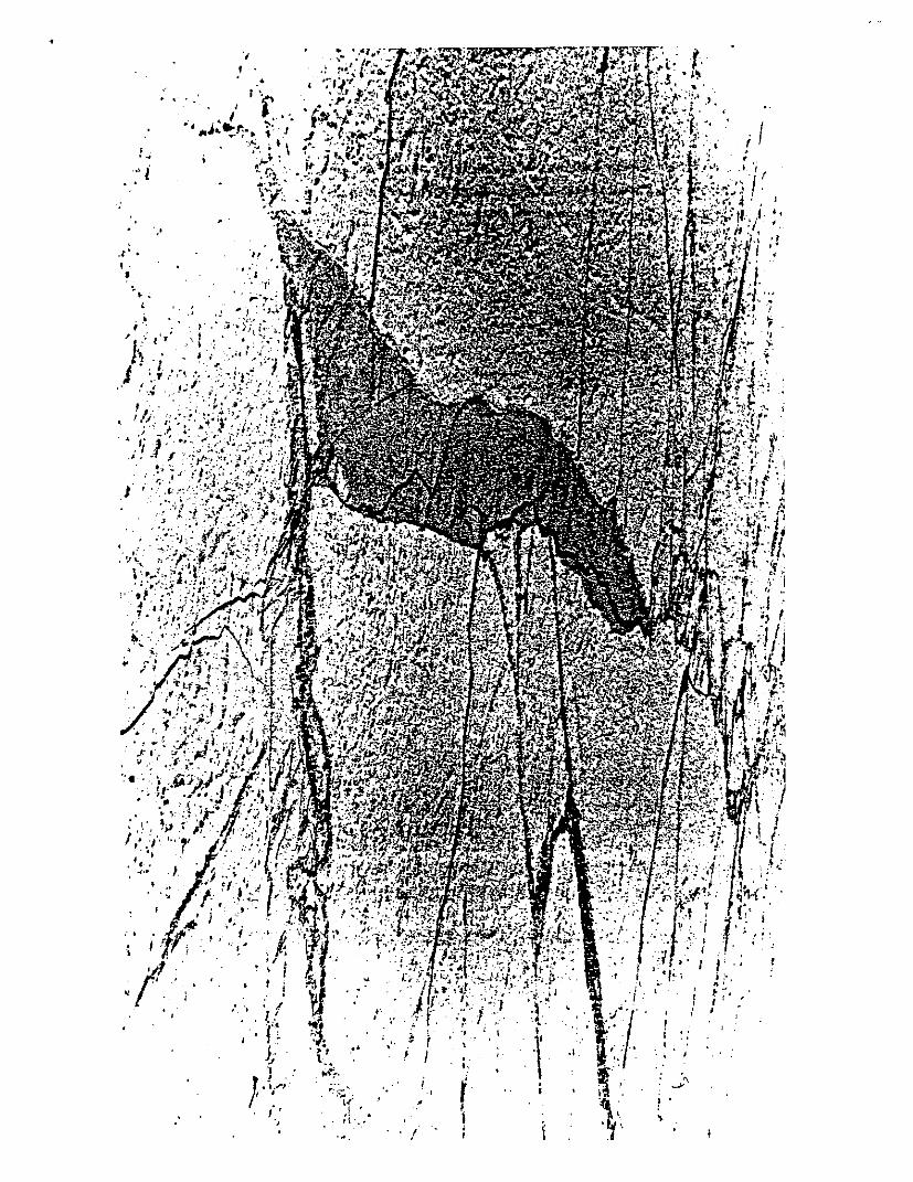
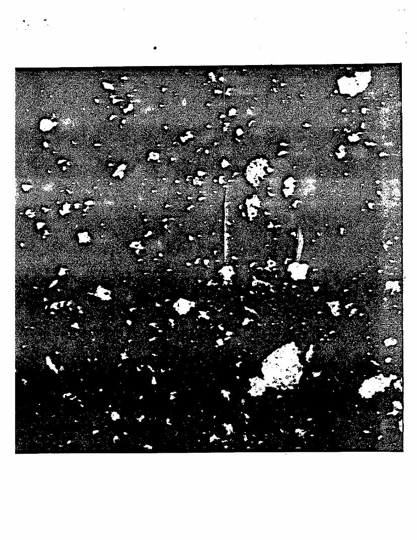
16

Iii

16

16

lC

I I I I

12 JULY 1979 I 719A-21031

●

● N=4.8x104~’”53

●

9

I I I I,03 ,04 ,05 , . 6 ,07 108

FLOE SIZE (m 2,

.?A- , .

I 1 I I I I 1’●

167 –

166 –

●

■

1 ci5 -

●

●

164 –

=1.23x166 e-14”4A

●

163 –

I I I 1- 1 . 4 0

I I I- 1 . 6 0 - 1 . 8 0 ‘ - 2 .00

POWER LAW EXPONENT (A)

POWER

1 I I

LAW EXPONENTI I I

“m “+ b

(A)I

+

.=+-

?●

1 ●

.