DAHAndbook Section 08p15 Impedance-Based-Fault-Location 757295 ENa

7/27/2019 DAHAndbook Section 08p15 Impedance-Based-Fault-Location 757295 ENa

http://slidepdf.com/reader/full/dahandbook-section-08p15-impedance-based-fault-location-757295-ena 1/24

Distribution Automation HandbookSection 8.15 Impedance-based Fault Location



Distribution Automation Handbook (prototype)

Power System Protection, 8.15 Impedance Based Fault Location

1MRS757295

2

Contents8.15 Impedance-based Fault Location ................................................................................................... 3

8.15.1 Introduction .............................................................................................................................. 3 8.15.2 Short Circuit Faults .................................................................................................................. 3

8.15.2.1 BASIC LOOP -MODELING METHOD .......................................................................................................................................... 3 8.15.2.1.1 Short circuit behind load or generation tap ....................... ........................ ........................ ........................ .............. 4 8.15.2.1.2 Short circuit in front of load or generation tap ....................................................................................................... 5

8.15.2.2 ADVANCED LOOP -MODELING METHOD .................................................................................................................................. 7 8.15.3 Earth Faults .............................................................................................................................. 9

8.15.3.1 BASIC LOOP -MODELING METHOD .......................................................................................................................................... 9 8.15.3.1.1 Earth fault behind load or generation tap ...................... ........................ ........................ ........................ ................ 11 8.15.3.1.2 Earth fault in front of load or generation tap ....................... ........................ ........................ ........................ ......... 12

8.15.3.2 ADVANCED LOOP -MODELING METHODS .............................................................................................................................. 14 8.15.3.2.1 Advanced loop model with load compensation ....................... ........................ ........................ ........................ ..... 14 8.15.3.2.2 Advanced load compensation method ...................... ........................ ........................ ........................ .................... 15 8.15.3.2.3 Load-modeling method ........................................................................................................................................ 18





1MRS757295

3

8.15 Impedance-based Fault Location

8.15.1 Introduction

As utilities today concentrate on continuity and reliability of their distribution networks, fault location has become an important supplementary function in modern IEDs. These fault location algorithms typically re-ly on the calculation of impedance from the fundamental frequency phasors measured in the substation.Therefore, it can be said that impedance-based methods have become an industry standard in this respect.The reason for their popularity is their easy implementation as they utilize the same signals as the other pro-tection and measurement functions in the IEDs. Their performance has been proven quite satisfactory in lo-cating short circuits, but improving further the performance in locating earth faults, especially in high-impedance earthed networks, is an on-going objective in the algorithm development.

Distribution networks have certain specific features which complicate and challenge fault location algo-rithms. These include, for example, non-homogeneity of lines, presence of laterals and load taps and thecombined effect of load current and fault resistance. Typical fault location algorithms are based on the as-sumption that the total load is tapped to the end point of the feeder, that is, the fault is always located infront of the load point. In real distribution feeders, this assumption is rarely correct. In fact, due to voltagedrop considerations, loads are typically located either in the beginning of the feeder or distributed more or less randomly over the entire feeder length. In such cases, fault location accuracy becomes easily deteri-orated unless somehow taken into account in the algorithm design. The effect of the above factors on theaccuracy becomes more substantial the lower the fault current magnitude in relation to the load current be-comes.

In the following, basic principles of impedance-based methods are introduced, and the performance of dif-ferent algorithm implementations is demonstrated using computer simulations.

8.15.2 Short Circui t Faults

8.15.2.1 Basic loop-modeling method

Like in distance protection, the impedance measurement is typically based on the concept of fault loops.The measured loop impedance used for the fault distance estimation is of the form:

LOOPSC

LOOPSC LOOPSC I

U Z _

_ _ = (8.15. 1)

Ideally Equation (8.15.1) produces the positive-sequence impedance 1 Z to the fault point.

The voltage LOOPSC U _ and current LOOPSC I _ are selected in accordance with the fault type. Table 8.15.1

shows a summary of the fault loops and applied voltages and currents in the impedance calculation for typ-ical short circuit faults.





1MRS757295

4

Table 8.15. 1: Voltages and currents used in the impedance calculation for short circuits

Fault type PhasesInvolved

Voltage LOOPSC U _ used in

loop impedance calculation

Current LOOPSC I _ used in


Phase-to-phase fault

A-B ABU AB I

B-C BC U BC I

C-A CAU CA I

Three-phase faultwith or without earth A-B-C(-E) ABU or BC U or CAU

AU or BU or C U AB I or BC I or CA I

A I or B I or C I

Because the possible fault resistance affects the measured fault loop impedance, the distance estimation isalways based on the reactive part of the LOOPSC Z _ , that is, LOOPSC X _ . This fault loop reactance is then con-

verted to physical distance by using the specified positive-sequence reactance value per kilometer of theconductor type of which the faulted feeder is composed.

However, especially in distribution networks the accuracy of the above loop model is also affected by theload current magnitude and its distribution along the feeder. These factors make the measured impedancefrom the IED location to appear typically too low. In case there is distributed generation along the feeder,this impedance can also be seen as too high. In the following, two basic scenarios are analyzed using sim-

plified circuit models.

8.15.2.1.1 Short circuit behind load or generation tap

Figure 8.15.1 shows a situation where a three-phase fault occurs behind a single load or distributed genera-tion tap.

Figure 8.15. 1: Three-phase fault occurs behind a single load or distributed generation tap

According to Figure 8.15.1, the equations for measured voltage and impedance from the IED location are:

PH LOADGEN F F LOOPSC

LOADGEN PH F LOADGEN PH PH LOOPSC

I I I R Z sd R Z d Z

I I I R I I I Z sd I Z sU

/))()((

)()()(

11 _

11 _

−+⋅−++⋅=

−+⋅+−+⋅⋅−+⋅⋅= (8.15. 2)

~

UPH

s·Z 1

IPH

d

(d-s)·Z 1

R FIFILOAD

~IGEN





1MRS757295

5

Equation (8.15.2) clearly shows the effect of the ratios PH LOAD I I and PH GEN I I together with a possible

fault resistance F R on the estimated impedance to the fault point when Equation (8.15.1) is used for esti-mation. In these cases, the correct impedance value would be F R Z d +1 .

8.15.2.1.2 Short circuit in front of load or generation tap

Figure 8.15.2 shows a situation where a three-phase fault occurs in front of a single load or distributed gen-eration tap.

Figure 8.15. 2: Three-phase fault occurs in front of a single load or distributed generation tap

According to Figure 8.15.2 the equations for measured voltage and impedance from the IED location are:

(8.15. 3)

Due to the fault and the resulting severe voltage collapse in front of the load tap, the load current compo-nent in Equation (8.15.3) can typically be neglected. With this assumption, the effect of possible fault resis-tance on the estimated fault loop impedance depends on the ratio PH GEN I I . As this ratio becomes lower,the estimated impedance to the fault point approaches its correct value F R Z d +1 .

The above schemes represent the problem as simplified, because in a real distribution feeder the load is dis-tributed along the feeder and multiple generation locations are possible. As a result, more complicated

schemes must be analyzed using computer simulations. The following example illustrates this.

)/)(1()(

1 _

1 _

PH LOADGEN F LOOPSC

LOADGEN PH F PH LOOPSC

I I I R Z d Z I I I R I Z d U

−+⋅+⋅=−+⋅+⋅⋅=





1MRS757295

6

Example 1 : The performance of the basic loop-modeling method is simulated in a feeder with the follow-ing data:

• 110/20 kV

Main transformer:

• S =20 MVA• K x =0.09 p.u

• Positive-sequence impedance,

Protected feeder:

1 Z , of the main line per unit length:

0.288+j0.284Ω

/km• Total load: 4 MVA (evenly distributed)

• Capacity: 1 MVA

Distributed generation (synchronous generator):

• D x′ =0.155 p.u• Operation mode: fixed ( )ϕ cos

A three-phase fault was simulated at steps of 0.1 p.u line length. The location of the distributed generationwas fixed to 0.5 p.u. The applied fault resistance represents the estimated maximum value of 2.5 Ω .





1MRS757295

7

Figure 8.15.3 shows the results.

Figure 8.15. 3: Simulated fault location estimates using the basic loop modeling method. Left: nodistributed generation, right: distributed generation included.

Considering the case without a distributed generation, it can be seen that the lower the ratio LOADPH I I Σ during the fault becomes, the higher is the error in the impedance estimation. This ratio decreases as thefault spot moves towards the end of the feeder. The current term LOAD I Σ is the total load current during thefault. When the distributed generation is included, the error at fault points behind the generation point is af-fected additionally by the ratio GEN PH I I . Typically, there will be an increase in the measured impedance ascan also be seen in this case. To mitigate the errors, load compensation together with the advanced loop-modeling method can be incorporated.

8.15.2.2 Advanced loop-modeling method

The calculation model of the basic loop-modeling method assumes that the same current flows througheach impedance element of the loop. As seen above, this assumption generates errors in the impedance es-timation. One way of improving the model is to use a different current quantity depending on the loop im-

pedance element in question. For example, estimate of the actual fault current is modeled to flow onlythrough the fault resistance, while the measured phase current is assumed to flow through the positive-sequence impedance of the feeder. This kind of modeling in fact introduces the load compensation feature.Figure 8.15.4 demonstrates this principle.

0 0.1 0.2 0.3 0.4 0.5 0.6 0.7 0.8 0.9 10

0.1

0.2

0.3

0.4

0.5

0.6

0.7

0.8

0.9

1

Fault distance (p.u)

E s

t i m a

t e d f a u

l t d i s t a n c e

( p . u

)

Short circuit location, no distr. generation

0 0.1 0.2 0.3 0.4 0.5 0.6 0.7 0.8 0.9 10

0.1

0.2

0.3

0.4

0.5

0.6

0.7

0.8

0.9

1


E s

t i m a

t e d f a u

l t d i s t a n c e

( p . u

)

No RFWith RF

Target

Short circuit location, distr. generation included

U AE , U BE , U CE

I A, IB, IC Z1, Z 2, Z 0

FL

ABC-f aul t

• Load evenly distr.:0.1 MVA/km• Main line: 40 km (1 p.u)

d

U AE , U BE , U CE

FL

ABC-f aul t

• Load evenly distr.:0.1 MVA/km• Main line: 40 km• Distr. gen. at d=0.5 p.u

IGEN

d

I A , IB, IC Z1, Z 2, Z 0

~

No RFWith RF

Target

Σ ILOADΣ ILOAD





1MRS757295

8

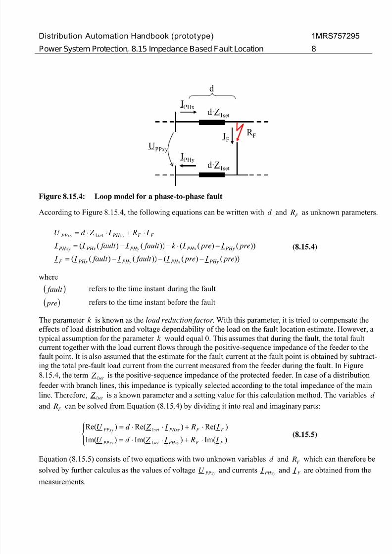
Figure 8.15. 4: Loop model for a phase-to-phase fault

According to Figure 8.15.4, the following equations can be written with d and F R as unknown parameters.

))()(())()((

))()(())()((1

pre I pre I fault I fault I I

pre I pre I k fault I fault I I

I R I Z d U

PHyPHxPHyPHxF

PHyPHxPHyPHxPHxy

F F PHxyset PPxy

−−−=

−⋅−−=

⋅+⋅⋅=

(8.15. 4)

where

( ) fault refers to the time instant during the fault( ) pre refers to the time instant before the fault

The parameter k is known as the load reduction factor . With this parameter, it is tried to compensate theeffects of load distribution and voltage dependability of the load on the fault location estimate. However, atypical assumption for the parameter k would equal 0. This assumes that during the fault, the total faultcurrent together with the load current flows through the positive-sequence impedance of the feeder to thefault point. It is also assumed that the estimate for the fault current at the fault point is obtained by subtract-ing the total pre-fault load current from the current measured from the feeder during the fault. In Figure8.15.4, the term lset Z is the positive-sequence impedance of the protected feeder. In case of a distribution

feeder with branch lines, this impedance is typically selected according to the total impedance of the mainline. Therefore, lset Z is a known parameter and a setting value for this calculation method. The variables d and F R can be solved from Equation (8.15.4) by dividing it into real and imaginary parts:

⋅+⋅⋅=

⋅+⋅⋅=

)Im()Im()Im(

)Re()Re()Re(

1

1

F F PHxyset PPxy

F F PHxyset PPxy

I R I Z d U

I R I Z d U (8.15. 5)

Equation (8.15.5) consists of two equations with two unknown variables d and F R which can therefore besolved by further calculus as the values of voltage PPxyU and currents PHxy I and F I are obtained from the

measurements.

d·Z 1set

IPHx

d

R FIF

IPHy

UPPxy

d·Z 1set





1MRS757295

9

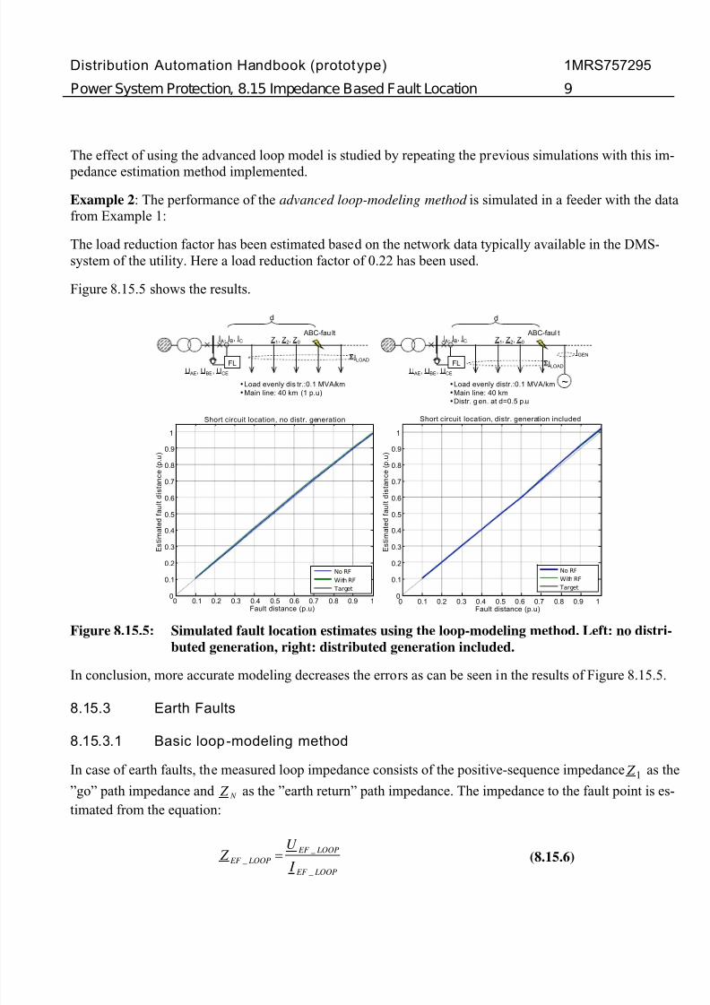
The effect of using the advanced loop model is studied by repeating the previous simulations with this im-

pedance estimation method implemented.Example 2 : The performance of the advanced loop-modeling method is simulated in a feeder with the datafrom Example 1:

The load reduction factor has been estimated based on the network data typically available in the DMS-system of the utility. Here a load reduction factor of 0.22 has been used.


Figure 8.15. 5: Simulated fault location estimates using the loop-modeling method. Left: no distri-buted generation, right: distributed generation included.

In conclusion, more accurate modeling decreases the errors as can be seen in the results of Figure 8.15.5.

8.15.3 Earth Faults

8.15.3.1 Basic loop-modeling method

In case of earth faults, the measured loop impedance consists of the positive-sequence impedance 1 Z as the

”go” path impedance and N Z as the ”earth return” path impedance. The impedance to the fault point is es-timated from the equation:

LOOP EF

LOOP EF LOOP EF I

U Z

_

_ _

= (8.15. 6)

E s

t i m a t e

d f a u

l t d i s t a n c e

( p . u

)

0 0.1 0.2 0.3 0.4 0.5 0.6 0.7 0.8 0.9 10

0.1

0.2

0.3

0.4

0.5

0.6

0.7

0.8

0.9

1


E s

t i m a t e

d f a u

l t d i s t a n c e

( p . u

)

Short circuit location, distr. generation included

0 0.1 0.2 0.3 0.4 0.5 0.6 0.7 0.8 0.9 10

0.1

0.2

0.3

0.4

0.5

0.6

0.7

0.8

0.9

1


No RFWith RF

Target

Short circuit location, no distr. generation

No RFWith RF

Target

U AE , U BE , U CE

I A , IB, IC Z1, Z 2, Z 0

FL

ABC-fau lt

• Load evenly dis tr.:0.1 MVA/km• Main line: 40 km (1 p.u)

d

U AE , U BE , U CE

FL

ABC-faul t

• Load evenly distr.:0.1 MVA/km• Main line: 40 km• Distr. g en. at d=0.5 p.u

IGEN

d

I A, IB, IC Z1, Z 2, Z 0

~

Σ ILOADΣ ILOAD





1MRS757295

10

Ideally, Equation (8.15.6) produces the sum of positive-sequence impedance 1 Z and the earth return path

impedance N Z to the fault point.

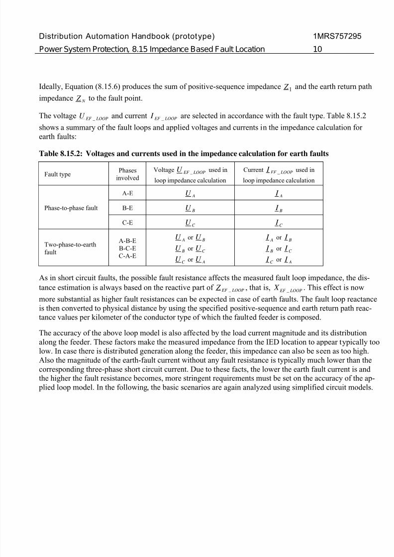
The voltage LOOP EF U _ and current LOOP EF I _ are selected in accordance with the fault type. Table 8.15.2

shows a summary of the fault loops and applied voltages and currents in the impedance calculation for earth faults:

Table 8.15. 2: Voltages and currents used in the impedance calculation for earth faults

Fault type Phasesinvolved

Voltage LOOP EF U _ used in


Current LOOP EF I _ used in


Phase-to-phase fault

A-E AU A I

B-E BU B I

C-E C U C I

Two-phase-to-earthfault

A-B-EB-C-EC-A-E

AU or BU

BU or C U

C U or AU

A I or B I

B I or C I

C I or A I

As in short circuit faults, the possible fault resistance affects the measured fault loop impedance, the dis-tance estimation is always based on the reactive part of LOOP EF Z _ , that is,

LOOP EF X

_ . This effect is now

more substantial as higher fault resistances can be expected in case of earth faults. The fault loop reactanceis then converted to physical distance by using the specified positive-sequence and earth return path reac-tance values per kilometer of the conductor type of which the faulted feeder is composed.

The accuracy of the above loop model is also affected by the load current magnitude and its distributionalong the feeder. These factors make the measured impedance from the IED location to appear typically toolow. In case there is distributed generation along the feeder, this impedance can also be seen as too high.Also the magnitude of the earth-fault current without any fault resistance is typically much lower than thecorresponding three-phase short circuit current. Due to these facts, the lower the earth fault current is and the higher the fault resistance becomes, more stringent requirements must be set on the accuracy of the ap-

plied loop model. In the following, the basic scenarios are again analyzed using simplified circuit models.





1MRS757295

11

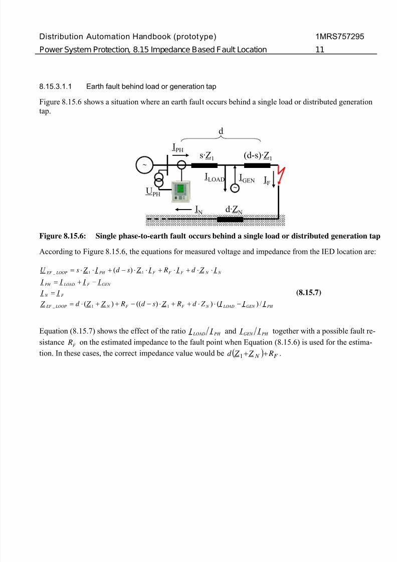
8.15.3.1.1 Earth fault behind load or generation tap

Figure 8.15.6 shows a situation where an earth fault occurs behind a single load or distributed generationtap.

Figure 8.15. 6: Single phase-to-earth fault occurs behind a single load or distributed generation tap

According to Figure 8.15.6, the equations for measured voltage and impedance from the IED location are:

PH GEN LOAD N F F N LOOP EF

F N

GEN F LOADPH

N N F F F PH LOOP EF

I I I Z d R Z sd R Z Z d Z I I

I I I I

I Z d I R I Z sd I Z sU

/)())(()(

)(

11 _

11 _

−⋅⋅++⋅−−++⋅==

−+=⋅⋅+⋅+⋅⋅−+⋅⋅=

(8.15. 7)

Equation (8.15.7) shows the effect of the ratio PH LOAD I I and PH GEN I I together with a possible fault re-sistance F R on the estimated impedance to the fault point when Equation (8.15.6) is used for the estima-tion. In these cases, the correct impedance value would be ( ) F N R Z Z d ++1 .

~

UPH

s·Z 1

IPH(d-s)·Z 1

IF

d·Z NI N

d

ILOAD~

IGEN





1MRS757295

12

8.15.3.1.2 Earth fault in front of load or generation tap

Figure 8.15.7 shows a situation where an earth fault occurs in front of a single load/distributed generationtap.

Figure 8.15. 7: Single phase-to-earth fault occurs in front of a single load or distributed generationtap

According to Figure 8.15.7, the equations for the measured voltage and impedance from the IED locationare:

PH GEN LOADF N F N LOOP EF

F N

GEN F LOADPH

N N F F PH LOOP EF

I I I R Z d R Z Z d Z

I I

I I I I

I Z d I R I Z d U

/)()()( 1 _

1 _

−⋅+⋅−++⋅=

=

−+=

⋅⋅+⋅+⋅⋅=

(8.15. 8)

It can be seen that even in case the load or generation is located in the end of the feeder, the simple modelof Equation (8.15.8) does not produce the correct result unless the phase current equals the fault current.

The above schemes represent the problem again as simplified, because in a real distribution feeder the load and the possible generation is distributed along the feeder, and therefore more complicated schemes must

be analyzed using computer simulations. The following example illustrates this.

Example 3 : The performance of the basic loop-modeling method is simulated in a feeder with the follow-ing data:

• 110/20 kV

Main transformer:

• S =20 MVA• K x =0.09 p.u• max EF I =1000 A (low-resistance earthing in the neutral point)

I N

~

UPH

IPHd·Z 1 (1-d)·Z 1

R FIF

d

d·Z N

ILOAD~

IGEN





1MRS757295

13


Protected feeder:

1 Z , of the main line per unit length:0.288+j0.284 Ω /km

• Zero-sequence impedance, 0 Z , of the main line per unit length:0.438+j2.006 Ω /km

• Earth return path impedance, N Z , of the main line per unit length:0.05+j0.574 Ω /km

• Total load: 4 MVA (evenly distributed)

•

Capacity: 1 MVA

Distributed generation (synchronous generator):

• D x′ =0.155 p.u• Operation mode: fixed ( )ϕ cos

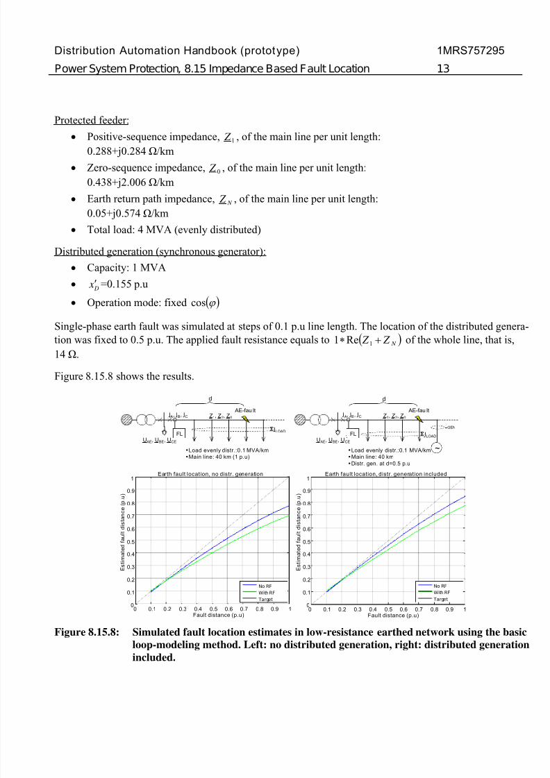
Single-phase earth fault was simulated at steps of 0.1 p.u line length. The location of the distributed genera-tion was fixed to 0.5 p.u. The applied fault resistance equals to ( ) N Z Z +∗

1Re1 of the whole line, that is,14 Ω .


Figure 8.15. 8: Simulated fault location estimates in low-resistance earthed network using the basicloop-modeling method. Left: no distributed generation, right: distributed generationincluded.

0 0.1 0.2 0.3 0.4 0.5 0.6 0.7 0.8 0.9 10

0.1

0.2

0.3

0.4

0.5

0.6

0.7

0.8

0.9

1


E s

t i m a

t e d f a u

l t d i s t a n c e

( p . u

)

Earth fault location, no distr. generation

0 0.1 0.2 0.3 0.4 0.5 0.6 0.7 0.8 0.9 10

0.1

0.2

0.3

0.4

0.5

0.6

0.7

0.8

0.9

1


E s

t i m a

t e d f a u

l t d i s t a n c e

( p . u

)

No RFWith RF

Target

Earth fault location, distr. generation included

U AE , U BE , U CE

I A , IB, IC Z1, Z 2, Z 0

FL

AE-fau lt


d

U AE , U BE , U CE

FL

AE-fau lt

• Load evenly distr.:0.1 MVA/km• Main line: 40 km• Distr. gen. at d=0.5 p.u

IGEN

d

I A, IB, IC Z1, Z 2, Z 0

~

No RFWith RF

Target

Σ ILOADΣ ILOAD





1MRS757295

14

The conclusion from the above simulation results is that basically the lower the ratio ( )GEN LOADPH I I I −Σ

becomes during the fault , the higher is the error in the impedance estimation. This ratio also equals( )PH F I I −11 , which clearly shows that if the measured phase current contains only the fault current, the

error is reduced to zero. Also increasing of the fault resistance increases this error. To mitigate the errors, amore advanced loop model with load compensation must be incorporated.

8.15.3.2 Advanced loop-modeling methods

8.15.3.2.1 Advanced loop model with load compensation

Improving of the model can be done using again different current quantities flowing through each imped-ance element. For example, estimate of the actual fault current is modeled to flow only through the fault re-sistance. Figure 8.15.9 demonstrates this.

Figure 8.15. 9: Loop model for phase-to-earth fault

According to Figure 8.15.9, the following equation can be written with d and F R as unknown parameters.

N Nset F F PHxset PEx I Z d I R I Z d U ⋅⋅+⋅+⋅⋅=1 (8.15. 9)

In Equation (8.15.9), N I and F I are estimations of the earth return path and fault currents respectively.Depending on the earthing method of the network, these currents can be estimated in different ways, but themost straightforward way is to assume that both N I and F I equal to the sum of the phase currents. Further in Equation (8.15.9), lset Z is the positive-sequence impedance of the protected feeder and Nset Z the imped-

ance of the earth return path. The latter impedance is calculated simply by ( ) 30 lset set Z Z − , where set Z 0 isthe zero-sequence impedance of the protected feeder. In case of a distribution feeder with branch lines,these impedances are typically selected according to the total impedance of the main line. Therefore, lset Z and Nset Z are known parameters and setting values for this calculation method. The variables d and F R can be solved from Equation (8.15.9) by dividing it into real and imaginary parts:

d·Z 1

IPHx

d

(1-d)·Z 1

R FIF

I Nd·Z N

UPHx

(1-d)·Z N





1MRS757295

15

⋅⋅+⋅+⋅⋅=⋅⋅+⋅+⋅⋅=

)Im()Im()Im()Im()Re()Re()Re()Re(

1

1

N Nset F F PHxset PHx

N Nset F F PHxset PHx

I Z d I R I Z d U I Z d I R I Z d U (8.15. 10)

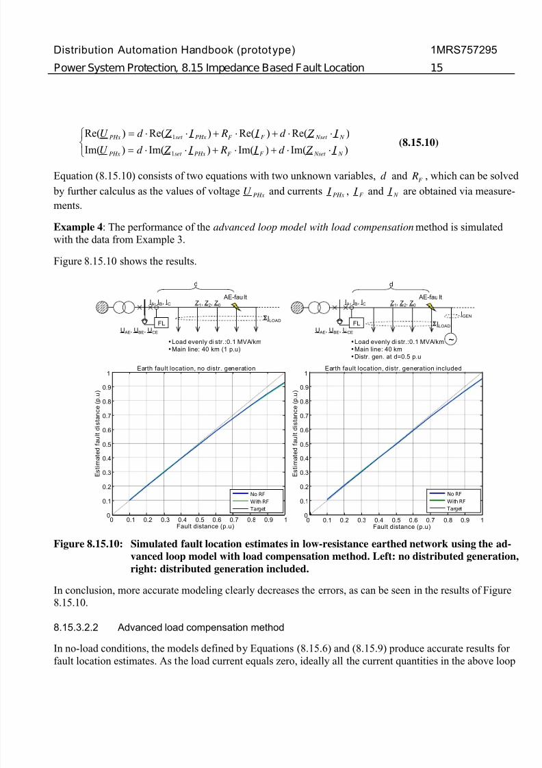
Equation (8.15.10) consists of two equations with two unknown variables, d and F R , which can be solved by further calculus as the values of voltage PHxU and currents PHx I , F I and N I are obtained via measure-ments.

Example 4 : The performance of the advanced loop model with load compensation method is simulated with the data from Example 3.


Figure 8.15. 10: Simulated fault location estimates in low-resistance earthed network using the ad-vanced loop model with load compensation method. Left: no distributed generation,right: distributed generation included.

In conclusion, more accurate modeling clearly decreases the errors, as can be seen in the results of Figure8.15.10.

8.15.3.2.2 Advanced load compensation method

In no-load conditions, the models defined by Equations (8.15.6) and (8.15.9) produce accurate results for fault location estimates. As the load current equals zero, ideally all the current quantities in the above loop

0 0.1 0.2 0.3 0.4 0.5 0.6 0.7 0.8 0.9 10

0.1

0.2

0.3

0.4

0.5

0.6

0.7

0.8

0.9

1


E s

t i m a

t e d f a u

l t d i s t a n c e ( p . u

)


0 0.1 0.2 0.3 0.4 0.5 0.6 0.7 0.8 0.9 10

0.1

0.2

0.3

0.4

0.5

0.6

0.7

0.8

0.9

1


E s

t i m a

t e d f a u

l t d i s t a n c e ( p . u

)

No RFWith RF

Target

Earth fault location, distr. generation included

U AE , U BE , U CE

I A, IB, IC Z1, Z 2, Z 0

FL

AE-fau lt

• Load evenly di str.:0.1 MVA/km• Main line: 40 km (1 p.u)

d

U AE , U BE , U CE

FL

AE-fau lt

• Load evenly di str.:0.1 MVA/km• Main line: 40 km• Distr. gen. at d=0.5 p.u

IGEN

d

I A , IB, IC Z1, Z 2, Z 0

~

No RFWith RF

Target

Σ ILOADΣ ILOAD





1MRS757295

16

models become equal, that is, F N PH I I I == , and therefore whichever of these current quantities can basi-

cally be used to calculate the impedance to the fault point simply by dividing the measured phase-to-earthvoltage of the faulted phase by this current. The advanced load compensation method makes use of this fact

by trying to compensate the effect of load from all related voltage and current sequence components meas-ured from the faulted feeder, and in this way the fault situation during normal load becomes reduced back to the corresponding no-load situation. The detailed description of this method is given in reference[8.15.1].

For the currents, the load compensation is done only for zero- and negative-sequence components accord-ing to Equation (8.15.11), because they can then be used directly for the distance estimation. The compen-sation thus removes the effect of load from the amplitudes and phase angles of these current phasors.

factor Lcomp Lcomp

factor Lcomp Lcomp

I I I I I I

_ 222

_ 000

+∆=+∆= (8.15. 11)

where

0 I ∆ is the measured change in the feeder zero-sequence current due to fault

2 I ∆ is the measured change in the feeder negative-sequence current due tofault

factor Lcomp I _ 0 is the calculated compensation factor for the feeder zero-sequence cur-rent

factor Lcomp I _ 2 is the calculated compensation factor for the feeder negative-sequencecurrent

Similarly for the sequence voltages it can be written:

factor Lcomp Lcomp

factor Lcomp Lcomp

factor Lcomp Lcomp

U U U

U U U

U U U

_ 222

_ 111

_ 000

+∆=+=

+∆=

(8.15. 12)

where

0U ∆ is the measured change in the zero-sequence voltage due to fault

2U ∆ is the measured change in the negative-sequence voltage due to fault

1U is the measured positive-sequence voltage during the fault

factor LcompU _ 0 is the calculated compensation factor for the zero-sequence voltage

factor LcompU _ 2 is the calculated compensation factor for the negative-sequence voltage

factor LcompU _ 1 is the calculated compensation factor for the positive-sequence voltage





1MRS757295

17

In the above equations the compensation factors for currents and voltages are estimated based on the meas-

ured positive-sequence current and changes in zero- and negative-sequence currents. In addition, also net-work data-based parameters such as phase-to-earth admittance values of the protected feeder and the back-ground network and the source impedance are utilized in the calculation. All these parameters can be esti-mated based on measurements during earth faults inside and outside the protected feeder.

After the compensation, the fault location can be done according to the equation:

Lcomp

Lcomp LOOP EF I

U Z

2 _

= (8.15. 13)

In the above equation, LcompU is the compensated phase-to-earth voltage of the faulted phase, for example,

Lcomp Lcomp Lcomp Lcomp U U U U 210++= is valid for the phase A.

The fault location is then based on the reactive part of LOOP EF Z _ , that is, LOOP EF X _ .

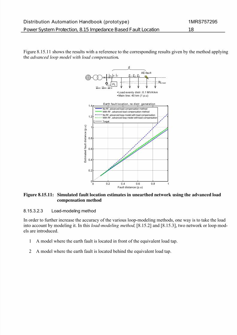
Example 5 : The performance of the advanced load compensation method is simulated in a feeder with thefollowing data:

• 110/20 kVMain transformer:

• S =20 MVA• K x =0.09 p.u

• Network:

max EF I =150 A (neutral point unearthed)


Protected feeder:

1 Z , of the main line per unit length:0.288+j0.284 Ω /km

• Zero-sequence impedance, 0 Z , of the main line per unit length:

0.438+j2.006 Ω /km• Earth return path impedance, N Z , of the main line per unit length:

0.05+j0.574 Ω /km• Total load: 4 MVA (evenly distributed)• No distributed generation included

Single-phase earth fault was simulated at steps of 0.1 p.u line length. The applied fault resistance equals to( ) N Z Z +∗

1Im5 of the whole line, that is, 170 Ω .





1MRS757295

18

Figure 8.15.11 shows the results with a reference to the corresponding results given by the method applying

the advanced loop model with load compensation .

Figure 8.15. 11: Simulated fault location estimates in unearthed network using the advanced loadcompensation method

8.15.3.2.3 Load-modeling method

In order to further increase the accuracy of the various loop-modeling methods, one way is to take the load into account by modeling it. In this load-modeling method, [8.15.2] and [8.15.3], two network or loop mod-els are introduced.

1 A model where the earth fault is located in front of the equivalent load tap.

2 A model where the earth fault is located behind the equivalent load tap.

U AE , U BE , U CE

I A, IB, IC Z1, Z 2, Z 0

FL

AE-fau lt


d

Σ ILOAD

0 0.2 0.4 0.6 0.8 10

0.2

0.4

0.6

0.8

1

1.2

1.4


E s

t i m a

t e d f a u

l t d i s t a n c e

( p . u

)


With RF, advanced loop model with load compensation

No RF, advanced load compensation method

Target

With RF, advanced load compensation methodNo RF, advanced loop model with load compensation





1MRS757295

19

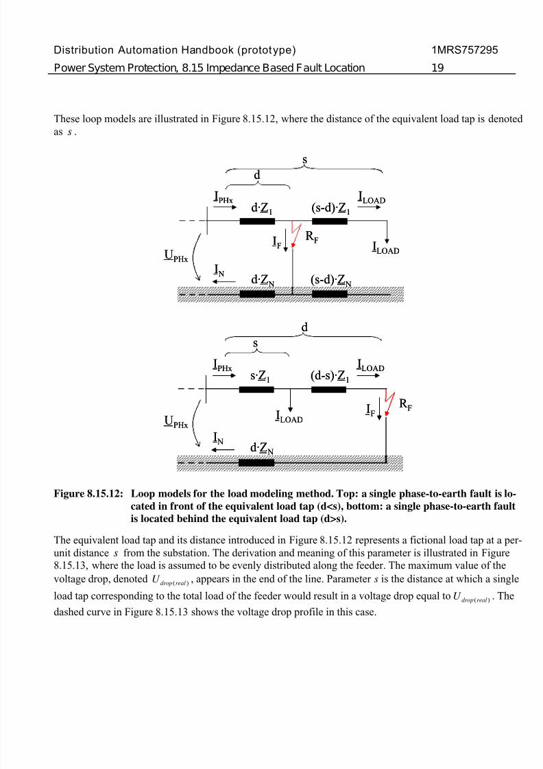
These loop models are illustrated in Figure 8.15.12, where the distance of the equivalent load tap is denoted

as s .

Figure 8.15. 12: Loop models for the load modeling method. Top: a single phase-to-earth fault is lo-cated in front of the equivalent load tap (d<s), bottom: a single phase-to-earth faultis located behind the equivalent load tap (d>s).

The equivalent load tap and its distance introduced in Figure 8.15.12 represents a fictional load tap at a per-unit distance s from the substation. The derivation and meaning of this parameter is illustrated in Figure8.15.13, where the load is assumed to be evenly distributed along the feeder. The maximum value of thevoltage drop, denoted )( realdropU , appears in the end of the line. Parameter s is the distance at which a single

load tap corresponding to the total load of the feeder would result in a voltage drop equal to )( realdropU . The

dashed curve in Figure 8.15.13 shows the voltage drop profile in this case.

d·Z 1

IPHx

d

(s-d)·Z 1

R FIF

I N d·Z N

ILOAD

s

s·Z 1

IPHx

s

(d-s)·Z 1

ILOAD

I N d·Z N

UPHx

ILOAD

d

R FIF

UPHxILOAD

(s-d)·Z N

d·Z 1

IPHx

d

(s-d)·Z 1

R FIF

I N d·Z N

ILOAD

s

s·Z 1

IPHx

s

(d-s)·Z 1

ILOAD

I N d·Z N

UPHx

ILOAD

d

R FIF

UPHxILOAD

(s-d)·Z N





1MRS757295

20

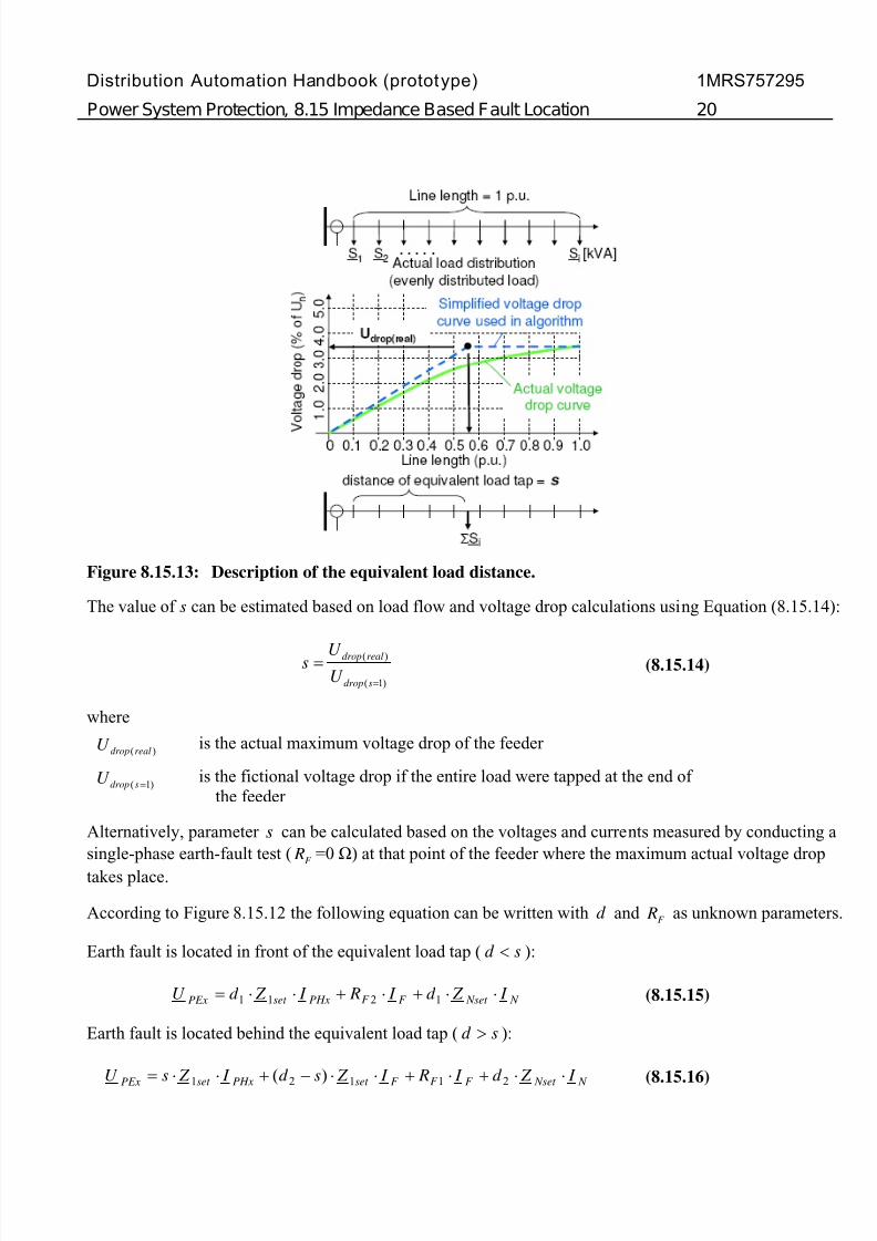
Figure 8.15. 13: Description of the equivalent load distance.

The value of s can be estimated based on load flow and voltage drop calculations using Equation (8.15.14):

)1(

)(

=

=sdrop

realdrop

U U s (8.15. 14)

where

)( realdropU is the actual maximum voltage drop of the feeder

)1( =sdropU is the fictional voltage drop if the entire load were tapped at the end of the feeder

Alternatively, parameter s can be calculated based on the voltages and currents measured by conducting asingle-phase earth-fault test ( F R =0 Ω ) at that point of the feeder where the maximum actual voltage droptakes place.

According to Figure 8.15.12 the following equation can be written with d and F R as unknown parameters.

Earth fault is located in front of the equivalent load tap ( sd < ):

N Nset F F PHxset PEx I Z d I R I Z d U ⋅⋅+⋅+⋅⋅=1211 (8.15. 15)

Earth fault is located behind the equivalent load tap ( sd > ):

N Nset F F

F set PHxset PExI Z d I R I Z sd I Z sU ⋅⋅+⋅+⋅⋅−+⋅⋅= 21

12

1)(

(8.15. 16)





1MRS757295

21

In Equations (8.15.15) and (8.15.16), N I and F I are estimations of the earth return path and fault currents

respectively. These currents can be modeled in different ways, but the most straightforward way is to as-sume that N I equals the sum of the phase currents, and that F I equals N I K ⋅ . The parameter K is the cur-rent distribution factor that takes into account the capacitive earth fault current contribution of the pro-tected feeder itself. Furthermore in Equations (8.15.15) and (8.15.16), lset Z is the positive-sequence imped-ance of the protected feeder and Nset Z the impedance of the earth return path. The latter impedance is cal-culated simply by ( ) 30 lset set Z Z − as before, where set Z 0 is the zero-sequence impedance of the protected feeder. In case of a distribution feeder with branch lines, these impedances are typically selected accordingto the total impedance of the main line. Therefore, lset Z and Nset Z are known parameters and setting valuesfor this calculation method. The variables 1d , 1F R and 2d , 2F R can be solved from Equations (8.15.15)

and (8.15.16) by dividing them into real and imaginary parts similarly as described already in Section8.15.3.2.1. As Equations (8.15.15) and (8.15.16) both need to be solved in parallel for each fault case, twosolutions, ld and 2d , for the distance estimate are always obtained. The logic for selecting between these

results is based on the calculated fault distance estimates: if 1d of Equation (8.15.15) is less than s , thenthis is the valid fault distance estimate, otherwise the distance estimate 2d is taken from Equation (8.15.16).

Example 6 : The performance of the load-modeling method is simulated with the data from Example 5. Theequivalent load distance has been estimated based on the network data typically available in the DMS-system of the utility. Here, an equivalent load distance of 0.47 has been used.





1MRS757295

22

Figure 8.15.14 shows the results with a reference to the corresponding results given by the method applying

the advanced load compensation method.

Figure 8.15. 14: Simulated fault location estimates in unearthed network using the load-modelingmethod

References

[8.15. 1] Wahlroos, A. & Altonen, J.

[

: "System and method for determininglocation of phase-to-earth fault," 20055232 F.3606FI 2041841FI.

8.15. 2] Wahlroos, A. & Altonen, J.

[

: "System and method for determininglocation of phase-to-earth fault," EP 06 127 343.9.

8.15. 3] Altonen, J. & Wahlroos, A.

: "Advancements in Fundamental FrequencyImpedance Based Earth-Fault Location in Unearthed Distribution

Networks," CIRED 19th International Conference on ElectricityDistribution, Vienna 2007.



Document revision history

Document revision/date History

A / 07 October 2010 First revision

Disclaimer and Copyrights

The information in this document is subject to change without notice and should not be construed as a commitment by ABBOy. ABB Oy assumes no responsibility for any errors that may appear in this document.

In no event shall ABB Oy be liable for direct, indirect, special, incidental or consequential damages of any nature or kind aris-ing from the use of this document, nor shall ABB Oy be liable for incidental or consequential damages arising from use of anysoftware or hardware described in this document.

This document and parts thereof must not be reproduced or copied without written permission from ABB Oy, and the contentsthereof must not be imparted to a third party nor used for any unauthorized purpose.

The software or hardware described in this document is furnished under a license and may be used, copied, or disclosed only inaccordance with the terms of such license.

Copyright © 2010 ABB Oy

All rights reserved.

TrademarksABB is a registered trademark of ABB Group. All other brand or product names mentioned inthis document may be trademarks or registered trademarks of their respective holders.



Documents

DAHAndbook Section 08p15 Impedance-Based-Fault-Location 757295 ENa