CZ4102 – High Performance Computing • Implicit Parallelism ...phytaysc/cz4102_08/cz4102_le2-3... · CZ4102 – High Performance Computing ... • Implicit Parallelism: Trends

1

CZ4102 CZ4102 –– High Performance ComputingHigh Performance Computing

Lectures 2 and 3: The Hardware Lectures 2 and 3: The Hardware ConsiderationsConsiderations

-- A/Prof Tay Seng ChuanA/Prof Tay Seng Chuan

Reference: ``Introduction to Parallel Computing'‘ – Chapter 2.

2

Topic Overview

• Implicit Parallelism: Trends in Microprocessor Architectures

• Limitations of Memory System Performance • Dichotomy of Parallel Computing Platforms • Communication Model of Parallel Platforms • Physical Organization of Parallel Platforms • Communication Costs in Parallel Machines • Messaging Cost Models and Routing Mechanisms • Mapping Techniques

3

Scope of Parallelism

• Different applications utilize different aspects of parallelism - e.g., data intensive applications utilize high aggregate throughput, server applications utilize high aggregate network bandwidth, and scientific applications typically utilize high processing and memory systemperformance.

• It is important to understand each of these performance bottlenecksand their interacting effect.

4

Implicit Parallelism: Trends in Microprocessor Architectures

• Current processors use these resources in multiple functional units

E.g.: Add R1, R2 (i) Instruction Fetch, (ii) Instruction Decode, (iii) Instruction Execute

• Consider these two instructions:Add R1, R2Add R2, R3

The precise manner in which these instructions are selected and executed provides impressive diversity in architectures with different performance and for different purpose. (Each architecture has its own merits and pitfalls.)

5

Pipelining and Superscalar Execution

• Pipelining overlaps various stages of instruction execution to achieve performance.

• At a high level of abstraction, an instruction can be executed while the next one is being decoded and the next one is being fetched.

• This is akin to an assembly line, e.g., for manufacture of cars.

6

Pipelining and Superscalar Execution • Pipelining, however, has several limitations. • The speed of a pipeline is eventually limited by the slowest stage.

• Conventional processors rely on very deep pipelines (20 stage pipelines in state-of-the-art Pentium processors).

• However, in typical program traces, every 5th to 6th instruction is a conditional jump (such as in if-else, switch-case)! This requires very accurate branch prediction.

• The penalty of a mis-prediction grows with the depth of the pipeline, since a larger number of instructions will have to be flushed.

20 Second 20 Second 130 Second 20 Second 20 Second

1 unit per

?? second

7

Pipelining and Superscalar Execution

• One simple way of alleviating these bottlenecks is to use multiple pipelines.

• Selecting which pipeline for execution becomes a challenge.

switch (…)

{ case 1:

case 2:

case 3:

case 4:

}

8

Superscalar Execution: An Example

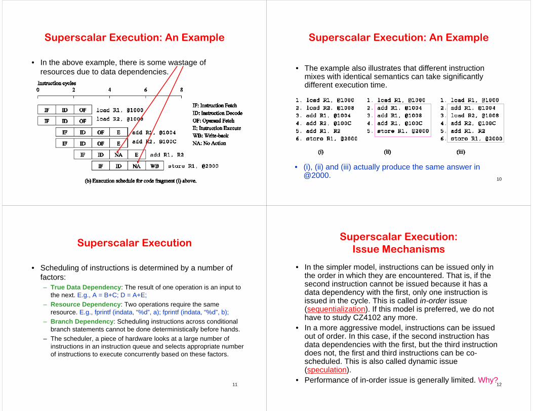
Example of a two-way superscalar execution of instructions.

9


• In the above example, there is some wastage of resources due to data dependencies.

10


• The example also illustrates that different instruction mixes with identical semantics can take significantly different execution time.

• (i), (ii) and (iii) actually produce the same answer in @2000.

11

Superscalar Execution

• Scheduling of instructions is determined by a number of factors: – True Data Dependency: The result of one operation is an input to

the next. E.g., A = B+C; D = A+E;– Resource Dependency: Two operations require the same

resource. E.g., fprintf (indata, “%d”, a); fprintf (indata, “%d”, b);– Branch Dependency: Scheduling instructions across conditional

branch statements cannot be done deterministically before hands.– The scheduler, a piece of hardware looks at a large number of

instructions in an instruction queue and selects appropriate number of instructions to execute concurrently based on these factors.

12

Superscalar Execution: Issue Mechanisms

• In the simpler model, instructions can be issued only in the order in which they are encountered. That is, if the second instruction cannot be issued because it has a data dependency with the first, only one instruction is issued in the cycle. This is called in-order issue (sequentialization). If this model is preferred, we do not have to study CZ4102 any more.

• In a more aggressive model, instructions can be issued out of order. In this case, if the second instruction has data dependencies with the first, but the third instruction does not, the first and third instructions can be co-scheduled. This is also called dynamic issue (speculation).

• Performance of in-order issue is generally limited. Why?

13

Superscalar Execution: Efficiency Considerations

• Not all functional units can be kept busy at all times. • If during a cycle, no functional units (FN) are utilized, this is referred to as

vertical waste.

• If during a cycle, only some of the functional units are utilized, this is referred to as horizontal waste.

• Due to limited parallelism in typical instruction traces, dependencies, or the inability of the scheduler to extract parallelism, the performance of superscalar processors is eventually limited.

• Conventional microprocessors typically support four-way superscalar execution.

FN1 FN2

14

Very Long Instruction Word (VLIW) Processors

• The hardware cost and complexity of the superscalar scheduler is a major consideration in processor design.

• To address this issues, VLIW processors rely on compile time analysis to identify and bundle together instructions that can be executed concurrently.

• These instructions are packed and dispatched together, and thus the name very long instruction word is used.

Div R1, R7Mul R2, R5Sub R4, R3Add R1, R2

4-Way VLIW

15

How to bundle (pack) the instructions in VLIW?

• Sequence of execution:add R1, R2 // add R2 to R1sub R2, R1 // subtract R1 from R3add R3, R4sub R4, R3

Solution:add R1, R2 sub R2,R1

add R3, R4 sub R4,R3

add R1, R2 add R3, R4

sub R2, R1 sub R4, R3

(1)

or

(2)

16

Very Long Instruction Word (VLIW) Processors: Considerations

• Hardware aspect is simpler. • Compiler has a bigger context from which to select co-

scheduled instructions. (More work for compiler.)• Compilers, however, do not have runtime information

such as cache misses. Scheduling is, therefore, inherently conservative.

• Branch and memory prediction is more difficult. • VLIW performance is highly dependent on the compiler.

A number of techniques such as loop unrolling, speculative execution, branch prediction are critical.

• Typical VLIW processors are limited to 4-way to 8-way parallelism.

17

Limitations of Memory System Performance

• Memory system, and not processor speed, is often the bottleneck for many applications.

• Memory system performance is largely captured by two parameters,latency and bandwidth.

• Latency is the time from the issue of a memory request to the time the data is available at the processor. (Waiting time until the first data is received. Consider the example of a fire-hose. If the water comes out of the hose two seconds after the hydrant is turned on, the latency of the system is two seconds. If you want immediate response from the hydrant, it is important to reduce latency. )

• Bandwidth is the rate at which data can be pumped to the processor by the memory system. (Once the water starts flowing, if the hydrant delivers water at the rate of 5 gallons/second, the bandwidth of the system is 5 gallons/second. If you want to fight big fires, you need a high bandwidth of water.)

18

Memory Latency: An Example

• Consider a processor operating at 1 GHz (1 ns clock) connected to a DRAM with a latency of 100 ns (no caches). Assume that the processor has two multiply-add units and is capable of executing four instructions in each cycle of 1 ns. The following observations follow:

– Since the memory latency is equal to 100 cycles and block size is one word, every time a memory request is made, the processor must wait 100 cycles before it can start to process the data. This is a serious drawback.

– The peak processor rating (assume no memory access) is computed as follows:Assume 4 instructions are executed on registers, peak processing rating = (4 Instructions)/(1 ns) = 4 GFLOPS. But this is not possible if memory access is needed. We will see it in the next slide.

GFLOPS: Giga Floating Point Operations per Second

19

Seriousness of Memory Latency• On the above architecture with memory latency of 100 ns, consider the

problem of computing a dot-product of two vectors.

(a1, a2, a3) (b1, b2, b3) = a1xb1 + a2xb2 + a3xb3

– A dot-product computation performs one multiply-add on a single pair of vector elements, i.e., each floating point operation requires one data fetch.

– It follows that the peak speed of this computation is limited to one floating point operation every 100 ns, ie, (1 FLOP)/(100 ns) = 1/(100 x 10-9 sec) FLOPS = 107 FLOPS = 10 x 106 FLOPS = 10 MFLOPS.

– The speed of 10 MFLOPS is a very small fraction of the peak processor rating (4 GFLOPS)!

20

Improving Effective Memory Latency Using Caches

• Caches are small and fast memory elements between the processor and DRAM.

• This memory acts as a low-latency high-bandwidth storage. • If a piece of data is repeatedly used, the effective latency of this

memory system can be reduced by the cache. • The fraction of data references satisfied by the cache is called the

cache hit ratio of the computation on the system. • Cache hit ratio achieved by a code on a memory system often

determines its performance. Eg: For 100 attempts to access to data in cache, if 30 attempts are successful, what is the cache hit ratio? What is the cache miss ratio? What is the impact if the cache miss ratio is greater than the cache hit ratio?

21

Impact of Memory Bandwidth

• Memory bandwidth is determined by the bandwidth (no. of bytes per second) of the memory bus as well as the memory units.

• Memory bandwidth can be improved by increasing the size of memory blocks. This will increase the size of the bus.

• It is important to note that increasing block size does not change latency of the system.

• In practice, wide data and address buses are expensive to construct.

• In a more practical system, consecutive words are sent on the memory bus on subsequent bus cycles after the first word is retrieved. This reduces latency by half.(Request for one word but receive two words.) 22

Impact of Memory Bandwidth

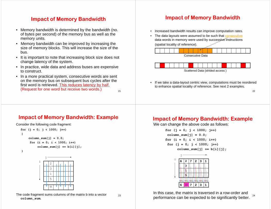
• Increased bandwidth results can improve computation rates. • The data layouts were assumed to be such that consecutive

data words in memory were used by successive instructions (spatial locality of reference).

• If we take a data-layout centric view, computations must be reordered to enhance spatial locality of reference. See next 2 examples.

Scattered Data (strided access )

Consecutive Data

23

Impact of Memory Bandwidth: Example Consider the following code fragment:

for (j = 0; j < 1000; j++) {

column_sum[j] = 0.0;for (i = 0; i < 1000; i++)

column_sum[j] += b[i][j];}

The code fragment sums columns of the matrix b into a vectorcolumn_sum.

5132

11

ji

24

Impact of Memory Bandwidth: ExampleWe can change the above code as follows:

for (j = 0; j < 1000; j++)column_sum[j] = 0.0;

for (i = 0; i < 1000; i++)for (j = 0; j < 1000; j++)

column_sum[j] += b[i][j];

In this case, the matrix is traversed in a row-order and performance can be expected to be significantly better.

513

132726

132726

ji

5611

25

Memory System Performance: Summary

• The series of examples presented in this section illustrate the following concepts: – Exploiting spatial and temporal locality in applications is critical

for amortizing memory latency and increasing effective memory bandwidth.

– Memory layouts and organizing computation (e.g., the two columnsum examples) appropriately can make a significant impact on the spatial and temporal locality.

26

Alternate Approaches for Hiding Memory Latency

• Consider the problem of browsing the web on a very slow network connection. We deal with the problem in one of three possible ways: – we anticipate which pages we are going to browse ahead of time

and issue requests for them in advance; – we open multiple browsers and access different pages in each

browser, thus while we are waiting for one page to load, we could be reading others; or

– we access a whole bunch of pages in one go - amortizing the latency across various accesses.

• The first approach is called prefetching, the second multithreading, and the third one corresponds to spatial locality in accessing memory words.

27

Multithreading for Latency Hiding

A thread is a single stream of control in the flow of a program. We illustrate threads with a simple example:

for (i = 0; i < n; i++)c[i] = dot_product(get_row(a, i), b);

Each dot-product is independent of the other, and therefore represents aconcurrent unit of execution. We can safely rewrite the above code segment as:

for (i = 0; i < n; i++)c[i] = create_thread(dot_product,get_row(a, i), b);

28

Multithreading for Latency Hiding: Example

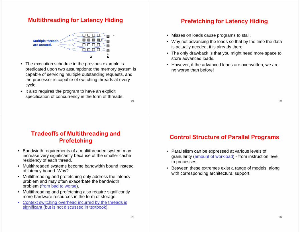
• In the code, the first instance of this function accesses a pair of vector elements and waits for them.

• In the meantime, the second instance of this function can accesstwo other vector elements in the next cycle, and so on.

• After l units of time, where l is the latency of the memory system, the first function instance gets the requested data from memory and can perform the required computation.

• In the next cycle, the data items for the next function instance arrive, and so on. In this way, in every clock cycle, we can perform a computation. This is how the memory latency is reduced.

Multiple threads are created.

29

Multithreading for Latency Hiding

• The execution schedule in the previous example is predicated upon two assumptions: the memory system is capable of servicing multiple outstanding requests, and the processor is capable of switching threads at every cycle.

• It also requires the program to have an explicit specification of concurrency in the form of threads.

Multiple threads are created.

30

Prefetching for Latency Hiding

• Misses on loads cause programs to stall. • Why not advancing the loads so that by the time the data

is actually needed, it is already there! • The only drawback is that you might need more space to

store advanced loads. • However, if the advanced loads are overwritten, we are

no worse than before!

31

Tradeoffs of Multithreading and Prefetching

• Bandwidth requirements of a multithreaded system may increase very significantly because of the smaller cache residency of each thread.

• Multithreaded systems become bandwidth bound instead of latency bound. Why?

• Multithreading and prefetching only address the latency problem and may often exacerbate the bandwidth problem (from bad to worse).

• Multithreading and prefetching also require significantly more hardware resources in the form of storage.

• Context switching overhead incurred by the threads is significant (but is not discussed in textbook).

32

Control Structure of Parallel Programs

• Parallelism can be expressed at various levels of granularity (amount of workload) - from instruction level to processes.

• Between these extremes exist a range of models, along with corresponding architectural support.

33

Control Structure of Parallel Programs

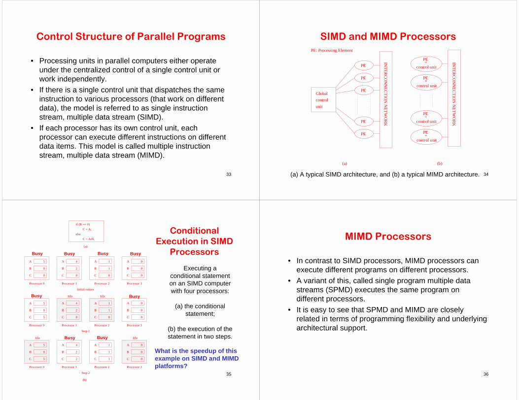
• Processing units in parallel computers either operate under the centralized control of a single control unit or work independently.

• If there is a single control unit that dispatches the same instruction to various processors (that work on different data), the model is referred to as single instruction stream, multiple data stream (SIMD).

• If each processor has its own control unit, each processor can execute different instructions on different data items. This model is called multiple instruction stream, multiple data stream (MIMD).

34

SIMD and MIMD Processors

(a) (b)

Global

+

+

+

+PE

PE

PE

PE

PE

PE

PE

PE

PE

control

unit

INT

ER

CO

NN

EC

TIO

N N

ET

WO

RK

INT

ER

CO

NN

EC

TIO

N N

ET

WO

RK

control unit

control unit

control unit

control unit

PE: Processing Element

(a) A typical SIMD architecture, and (b) a typical MIMD architecture.

35

Conditional Execution in SIMD

Processors

Idle

Idle

(b)

Step 2

(a)

Idle

Step 1

Initial values

Idle

C

B

0

A

B

C 0

A

B

C0

A

B

A

0

else

C

Processor 0 Processor 1 Processor 2

5

0

4

2

1

1

0

0

A

B

C 0

A

B

C

A

B

C 0

A

B

C5 0

C = A/B;

C = A;

if (B == 0)

Processor 3

Processor 0 Processor 1 Processor 2 Processor 3

5

0

4

2

1

1

0

0

Processor 0 Processor 1 Processor 2 Processor 3

5

0

4

2

1

1

0

0

0

A

B

C

A

B

C

A

B

C

A

B

C 5 12

Executing a conditional statement on an SIMD computer with four processors:

(a) the conditional statement;

(b) the execution of the statement in two steps.

Busy Busy Busy Busy

Busy Busy

Busy Busy

What is the speedup of this example on SIMD and MIMD platforms?

36

MIMD Processors

• In contrast to SIMD processors, MIMD processors can execute different programs on different processors.

• A variant of this, called single program multiple data streams (SPMD) executes the same program on different processors.

• It is easy to see that SPMD and MIMD are closely related in terms of programming flexibility and underlying architectural support.

37

Communication Model of Parallel Platforms

• There are two primary forms of data exchange between parallel tasks - accessing a shared data space and exchanging messages.

Shared MemoryShared Memory

CPUCPU CPUCPU CPUCPU……

• Platforms that provide a shared data space are called shared-address-space machines or multiprocessors.

• Platforms that support messaging are also called message passing platforms or multicomputers. 38

Shared-Address-Space vs.

Shared Memory Machines

• It is important to note the difference between the terms shared address space and shared memory.

• Shared address space is a programming abstraction.• Shared memory is a physical machine attribute. • It is possible to provide a shared address space using a

physically distributed memory.

39

Message-Passing Platforms

• These platforms comprise of a set of processors and their own (exclusive) memory.

• Instances of such a view come naturally from clustered workstations and non-shared-address-space multicomputers.

• These platforms are programmed using (variants of) send and receive primitives.

• Libraries such as MPI (Message Passing Interface) and PVM (Parallel Virtual Machine) provide such primitives.

• In this course only MPI is taught.

40

Architecture of an Ideal Parallel Computer

• A natural extension of the Random Access Machine (RAM) serial architecture is the Parallel Random Access Machine, or PRAM. We begin this discussion with an ideal parallel machine called Parallel Random Access Machine, or PRAM.

• PRAMs consist of p processors and a global memory of unbounded size that is uniformly accessible to all processors.

• Processors share a common clock but may execute different instructions in each cycle.

• These are merely theoretical models.

41

Architecture of an Ideal Parallel Computer

• Depending on how simultaneous memory accesses are handled, PRAMs can be divided into four subclasses. – Exclusive-read, exclusive-write (EREW) PRAM. – Concurrent-read, exclusive-write (CREW) PRAM. – Exclusive-read, concurrent-write (ERCW) PRAM. – Concurrent-read, concurrent-write (CRCW) PRAM.

• What does concurrent write mean, anyway? It depends on the semantic (meaning):– Common: write only if all values are identical. – Arbitrary: write the data from a randomly selected processor. – Priority: follow a predetermined priority order. – Sum: Write the sum of all data items.

42

Interconnection Networks for Parallel Computers

• Interconnection networks carry data between processors and to memory.

• Interconnectors are made of switches and links (wires, fiber).

• Interconnectors are classified as static or dynamic. • Static networks consist of point-to-point communication

links among processing nodes and are also referred to as direct networks. Its configuration cannot be changed.

• Dynamic networks are built using switches and communication links. Dynamic networks are also referred to as indirect networks. Its configuration can be changed.

43

Static and DynamicInterconnection Networks

Static network Indirect network

Switching elementProcessing node

Network interface/switch

P

P P P

P

P

PP

Classification of interconnection networks: (a) a static network; and (b) a dynamic network.

(a) (b)

fixed

44

Interconnection Networks

• Switches map a fixed number of inputs to outputs. • The total number of ports (input + output) on a switch is

the degree of the switch.

Degree of the switch = ?

45

Network Topologies

• A variety of network topologies have been proposed and implemented.

• These topologies tradeoff performance for cost. • Commercial machines often implement hybrids of

multiple topologies for reasons of packaging, cost, fault tolerance and available components. These requirements can be conflicting.

46

Network Topologies: Buses

• Some of the simplest and earliest parallel machines used buses.

• All processors access a common bus for exchanging data.

• The distance between any two nodes is O(1) in a bus. The bus also provides a convenient broadcast media.

• However, the bandwidth of the shared bus is a major bottleneck.

47

Network Topologies: Buses

Cache /Local Memory

Cache /Local Memory

Shar

ed M

emor

y

Data

Processor 0

Address

Data

Shar

ed M

emor

y

Processor 0 Processor 1

(a)

(b)

Address

Processor 1

Bus-based interconnects (a) with no local caches; (b) with local memory/caches.

Since much of the data accessed by processors is local to the processor, a local memory can improve the performance of bus-based machines. 48

Network Topologies: Crossbars

A completely non-blocking crossbar network connecting p processors to b memory banks.

A crossbar network uses an p×m grid of switches to connect p inputs to m outputs in a non-blocking manner.

Memory Banks

b−1543210

Proc

essi

ng E

lem

ents

0

1

2

3

4

5

6

p−1

elementA switching

Cross Bar Network

A switching element

49

Network Topologies: Multistage Networks

• Crossbars have excellent performance scalability but poor cost scalability.

• Buses have excellent cost scalability, but poor performance scalability.

• A Multistage Interconnection Network strikes a compromise between these extremes.

111

110

101

100

011

010

001

000 000

001

010

011

100

101

110

111 50

Network Topologies: Multistage Networks

Memory banks

0

1

0

. . . . . . . . . . . . . . . . . . . .

.

.

.

.

.

.

.

.

.

.

.

.

.

.

.

.

.

.

.

.

Stage 1

b-1

Stage 2 Stage n

p-1

Processors Multistage interconnection network

1

The schematic of a typical multistage interconnection network.

51

Network Topologies: Multistage Omega Network

• One of the most commonly used multistage interconnects is the Omega network.

• This network consists of log p stages, where p is the number of inputs/outputs.

• At each stage, input i is connected to output j if:

52


Each stage of the Omega network implements a perfect shuffle as follows:

A perfect shuffle interconnection for eight inputs and outputs (p=8).

000

010

100

110

001

011

101

111

000

010

100

110

001

011

101

111

0

1

2

3

4

5

6

7

0

1

2

3

4

5

6

7

= left_rotate(000)

= left_rotate(100)

= left_rotate(001)

= left_rotate(101)

= left_rotate(010)

= left_rotate(110)

= left_rotate(011)

= left_rotate(111)

i j

53


• The perfect shuffle patterns are connected using 2×2 switches.

• The switches operate in two modes – crossover or passthrough (straight).

(b)(a)

Two switching configurations of the 2 × 2 switch: (a) Pass-through (straight); (b) Cross-over.

54


A complete omega network connecting eight inputs and eight outputs.

An omega network has p/2 × log p switching nodes, and the cost of such a network grows as O(p log p).

A complete Omega network with the perfect shuffle interconnects and switches can now be illustrated:

111

110

101

100

011

010

001

000 000

001

010

011

100

101

110

111

55

Network Topologies: Multistage Omega Network – Routing

• Let s be the binary representation of the source and d be that of the destination processor.

• The data traverses the link to the first switching node. If the most significant bits of s and d are the same, then the data is routed in pass-through mode by the switch else, it switches to crossover.

• This process is repeated for each of the log p switching stages.

• Note that this is not a non-blocking switch.

56

Network Topologies: Multistage Omega Network – Routing

An example of blocking in omega network: one of the messages (010 to 111, or, 110 to 100) is blocked at link AB.

111

110

101

100

011

010

001

000 000

001

010

011

100

101

110

111

A

B

(010 to 111) : cross, straight, cross

(110 to 100) : straight, cross, straight

57

Network Topologies: Completely Connected Network

• Each processor is connected to every other processor.• The number of links in the network scales as O(p2).• While the performance scales very well, the hardware

complexity is not realizable for large values of p.• In this sense, these networks are static counterparts of

crossbars.

58

Network Topologies: Star Connected Network

• Every node is connected only to a common node at the center.

• Distance between any pair of nodes is O(1). However, the central node becomes a bottleneck.

• In this sense, star connected networks are static counterparts of buses.

59

Network Topologies: Linear Arrays, Meshes, and k-d Meshes

• In a linear array, each node has two neighbors, one to its left and one to its right. If the nodes at either end are connected, we refer to it as a 1-D torus or a ring.

Linear arrays: (a) with no wraparound links; (b) with wraparound link.

(a) (b)

60


• A generalization to 2 dimensions has nodes with 4 neighbors, to the north, south, east, and west.

• A further generalization to d dimensions has nodes with 2dneighbors.

Two and three dimensional meshes: (a) 2-D mesh with no wraparound; (b) 2-D mesh with wraparound link (2-D torus); and

(c) a 3-D mesh with no wraparound.

(c)(b)(a)

61


• A special case of a d-dimensional mesh is a hypercube. Here, d = log p, where p is the total number of nodes.

Construction of hypercubes from

hypercubes of lower dimension.

0

1

00

01

10

11

000 010

001 011

100 110

111101

0000

0100

0001 0011

0101

0110

0010

0111

1100 1110

1111

10111001

1000

1101

1010

0-D hypercube 1-D hypercube 2-D hypercube 3-D hypercube

4-D hypercube

62

Network Topologies: Properties of Hypercubes

• The distance between any two nodes is at most log p.• Each node has log p neighbors.• The distance between two nodes is given by the number

of bit positions at which the two nodes differ. The path is not unique for d > 2.

Distance from 0000 to 1000 =1

Distance from 0100 to 1011 = 4

63

Network Topologies: Tree-Based Networks

Complete binary tree networks: (a) a static tree network; and (b) a dynamic tree network.

(a) (b)

Processing nodes

Switching nodes

64

Network Topologies: Tree Properties • The distance between any two nodes is no more than

2 log p.

• Links higher up the tree potentially carry more traffic than those at the lower levels.

• For this reason, a variant called a fat-tree, fattens the links as we go up the tree.

• Trees can be laid out in 2D with no wire crossings. This is an attractive property of trees.

p

65

Network Topologies: Fat Trees

A fat tree network of 16 processing nodes.

fat

fatter

Very fat

These fats will take care of the bottleneck closer to the root.

66

Evaluating Static Interconnection Networks

• Diameter: The distance between the farthest two nodes in the network. Thediameter of a linear array is p − 1, that of a mesh is 2( − 1),that of a tree is 2(log p) (worst case is p-1),that of hypercube is log p, and that of a completely connected network is O(1).

(p-1)

67


• Bisection Width (may not have a picture to represent): The minimum number of wires you must cut to divide the network into two equal parts. The bisection width of a linear array and tree is 1, that of a mesh is , that of a hypercube is p/2 and that of a completely connected network is p2/4.

68


Bisection Width for Linear Array

Given p nodes, total number of links = p-1.

For each half network, the number of nodes is p/2.

The number of links in each half network is (p/2 - 1).

The number of links to be removed from linear array is

(p-1) – 2 x (p/2 -1) = p-1 – p + 2 = 1.

p nodes

p/2 nodes p/2 nodes

69


• Cost: The number of links or switches (whichever is asymptotically higher) is a meaningful measure of the cost. However, a number of other factors, such as the ability to layout the network, the length of wires, etc., also factor in tothe cost.

70

Cache Coherence in Multiprocessor Systems

• Interconnection networks provide basic mechanisms for data transfer.

• The underlying technique must provide some guarantees on the semantics – data integrity must be ensured.

• This guarantee is generally one of serializability, i.e., there exists some serial order of instruction execution that corresponds to the parallel schedule.

71

Cache Coherence in Multiprocessor Systems

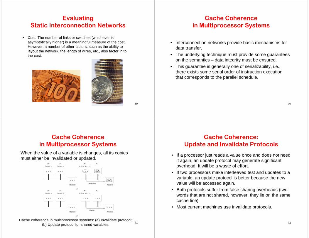
Cache coherence in multiprocessor systems: (a) Invalidate protocol; (b) Update protocol for shared variables.

When the value of a variable is changes, all its copies must either be invalidated or updated.

(b)

(a)

InvalidateMemoryMemory

P1P0P1P0

UpdateMemoryMemory

P1P0P1P0

load x

write #3, xload xload x

x = 1

x = 1x = 1

x = 1

x = 1x = 1

x = 3

x = 3

x = 3x = 3

x = 1

x = 1

write #3, xload x

72

Cache Coherence: Update and Invalidate Protocols

• If a processor just reads a value once and does not need it again, an update protocol may generate significant overhead. It will be a waste of effort.

• If two processors make interleaved test and updates to a variable, an update protocol is better because the new value will be accessed again.

• Both protocols suffer from false sharing overheads (two words that are not shared, however, they lie on the same cache line).

• Most current machines use invalidate protocols.

73

Maintaining Coherence Using Invalidate Protocols

• Each copy of a data item is associated with a state.

• One example of such a set of states is, shared, invalid, or dirty.

• In shared state, there are multiple valid copies of the data item (and therefore, an invalidate would have to be generated on an update).

• In dirty state, only one copy exists and therefore, no invalidates need to be generated.

• In invalid state, the data copy is invalid, therefore, a read generates a data request (and associated state changes).

(b)

(a)

InvalidateMemoryMemory

P1P0P1P0

UpdateMemoryMemory

P1P0P1P0

load x

write #3, xload xload x

x = 1

x = 1x = 1

x = 1

x = 1x = 1

x = 3

x = 3

x = 3x = 3

x = 1

x = 1

write #3, xload x

74


flush

read/write

read write

C_read

read

C_write

write

C_write

Dirty

Shared

Invalid

State diagram of a simple three-state coherence protocol.

(throw away wrong data)c_write, c_read : write and read operations

performed by remote node

75


y = 13, D

y = 13, S

x = 6, S

x = 6, I

y = 19, D

y = 20, D

x = 5, S

y = 12, S

x = 5, I

y = 12, I

y = 13, S

x = 6, S

y = 13, I

x = 6, I

y = 13, I

x = 5, D

y = 12, D

x = 6, I

read x

x = x + 1

x = x + y

x = x + 1

read y

y = y + 1

read x

y = x + y

read y

y = 12, S

y = 13, I

x = 19, D

x = 6, S

x = 20, D

y = 13, S

x = 6, D

x = 5, S

y = y + 1

Processor 0

Variables andtheir states atProcessor 1

Variables andtheir states inProcessor 1Global mem.

Instruction atProcessor 0

Instruction atTimetheir states atVariables and

Example of parallel program execution with the simplethree-state coherence protocol.

flush

read/write

read write

C_read

read

C_write

write

C_write

Dirty

Shared

Invalid

32

33

76

Snoopy Cache Systems

Snoopy is Snoopy is nosy!!nosy!!

We are making use of this nosyWe are making use of this nosy--ness ness (busy body(busy body--nessness) to ensure the integrity ) to ensure the integrity of cache data.of cache data.

77

Snoopy Cache Systems

How are invalidates sent to the right processors?

In snoopy caches, there is a broadcast media that listens to all invalidates and read requests and performs appropriate coherence operations locally.

A simple snoopy bus based cache coherence system.

Tag

s

Snoo

p H

/W

Processor

CacheT

ags

Snoo

p H

/WProcessor

Cache

Tag

s

Snoo

p H

/W

Processor

Cache

Dirty

Address/data

Memory

78

Performance of Snoopy Caches

• Once copies of data are tagged dirty (have been altered), all subsequent operations can be performed locally (use the latest values) on the cache without generating external traffic.

• If a data item is read by a number of processors, it is changed to shared state in the cache and all subsequent read operations become local (data has been acquired).

• If processors read and update data at the same time, they generate coherence requests on the bus (to update the other copy) - which is ultimately bandwidth limited.

Tag

s

Snoo

p H

/W

Processor

Cache

Tag

s

Snoo

p H

/W

Processor

Cache

Tag

s

Snoo

p H

/W

Processor

Cache

Dirty

Address/data

Memory

79

Communication Costs in Parallel Machines

• Along with idling and contention, communication is a major overhead in parallel programs.

• The cost of communication is dependent on a variety of features including the programming model semantics, the network topology, data handling and routing, and associated software protocols.

80

Message Passing Costs in Parallel Computers

• The total time to transfer a message over a network comprises of the following:– Startup time (ts): Time spent at sending and receiving nodes to

set up communication link (executing the routing algorithm, programming routers, etc.).

– Per-hop time (th): This time is a function of number of hops and includes factors such as switch latencies, network delays, etc.

– Per-word transfer time (tw): This time includes all overheads that are determined by the length of the message. This includes bandwidth of links, error checking and correction, etc.

81

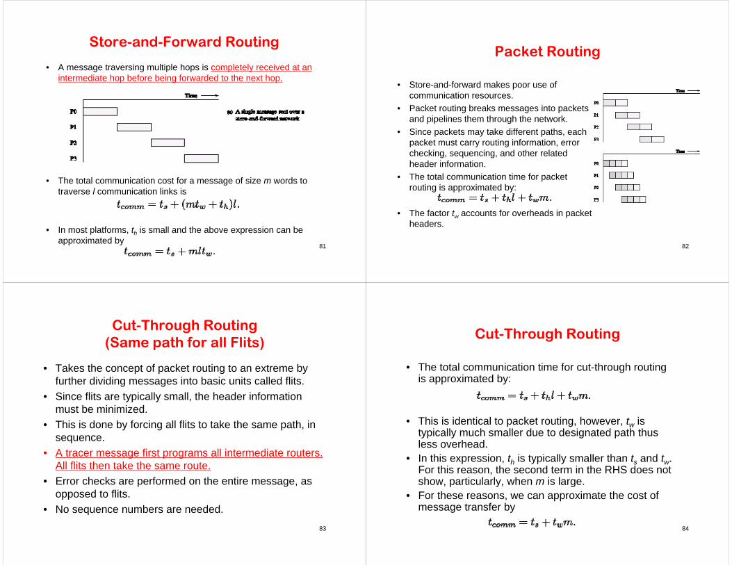
Store-and-Forward Routing

• A message traversing multiple hops is completely received at an intermediate hop before being forwarded to the next hop.

• The total communication cost for a message of size m words to traverse l communication links is

• In most platforms, th is small and the above expression can be approximated by

82

Packet Routing

• Store-and-forward makes poor use of communication resources.

• Packet routing breaks messages into packets and pipelines them through the network.

• Since packets may take different paths, each packet must carry routing information, error checking, sequencing, and other related header information.

• The total communication time for packet routing is approximated by:

• The factor tw accounts for overheads in packet headers.

83

Cut-Through Routing (Same path for all Flits)

• Takes the concept of packet routing to an extreme by further dividing messages into basic units called flits.

• Since flits are typically small, the header information must be minimized.

• This is done by forcing all flits to take the same path, in sequence.

• A tracer message first programs all intermediate routers. All flits then take the same route.

• Error checks are performed on the entire message, as opposed to flits.

• No sequence numbers are needed. 84

Cut-Through Routing

• The total communication time for cut-through routing is approximated by:

• This is identical to packet routing, however, tw is typically much smaller due to designated path thus less overhead.

• In this expression, th is typically smaller than ts and tw. For this reason, the second term in the RHS does not show, particularly, when m is large.

• For these reasons, we can approximate the cost of message transfer by

85

Routing Mechanisms for Interconnection Networks

• How does one compute the route that a message takes from source to destination?

– Routing must prevent deadlocks - for this reason, we use dimension-ordered or e-cube routing, i.e., precedence will need to be defined, e.g., x+, x-, y+, y-, z+, z-.

– Routing must avoid hot-spots - for this reason, two-step routing is often used. In this case, a message from source s to destination d is first sent to a randomly chosen intermediate processor i and then forwarded to destination d.

Routing a message from node Ps (010) to node Pd (111) in a three-dimensional hypercube using E-cube routing.

Step 2 (110 111)Step 1 (010 110)

pdpdpd

pspsps

111110

101

011

100

010

001000

111110

101

011

100

010

001001000

010

101100

011

110 111

000

011) (011 -> 111)

86

Mapping Techniques for Graphs

• The reality is not that rosy. Often, we need to embed a known communication pattern into a given interconnection topology.

• We may have an algorithm designed for one network. But this algorithm will need to be working on another topology in the implementation platform.

• For these reasons, it is useful to understand mapping between graphs.

87

Mapping Techniques for Graphs: Metrics

• When mapping a graph G(V,E) into G’(V’,E’), the following metrics are important:

• The maximum number of edges mapped onto any edge in E’ is called the congestion of the mapping.

1

2

3

4

56

1’

2’

3’

4’

5’

6’

congestion of the mapping = 5

G G’

7

7’88


• The maximum number of links in E’ that any edge in E ismapped onto is called the dilation of the mapping.

1

2

31’

2’2

3’3’ 3

3’

3’

G G’

dilation of the mapping = 5 (good fault tolerance)

X X’

YY’

Y’

Z

Z’

Z’Z’

Z’

W

W’

Z’

89


• The ratio of the number of nodes in the set V’ to that in set V is called the expansion of the mapping.

G G’

expansion of the mapping = 7/4 = 1.7590

Embedding a Linear Array into a Hypercube

• A linear array (or a ring) composed of 2d nodes (labeled 0 through 2d − 1) can be embedded into a d-dimensional hypercube by mapping node i of the linear array onto node in hypercube.

• G(i, d) of the hypercube refers to the i th entry in the sequence of Gray codes of d bits. The function G(i, x) is defined as follows:

0

91


110G(4,3) = 22 + G(2 2+1 -1 -4, 2) = 4 + G(8-1-4, 2) = 4+ G(3,2) =4 + (21 + G(21+1 -1 – 3, 1) ) = 4 + (2 + G(0,1)) = 4 + (2+0) = 6

4

010G(3,3) = G(3,2) = 21 + G(2 1+1 – 1 – 3, 1) = 2 + G(0,1) = 2+0 = 2(3 < 4) 3 >= 2)

3

011G(2,3) = G(2,2) = 21 + G(2 1+1 – 1 – 2, 1) = 2 + G(1,1) = 2+1 = 3(2 < 4) (2 >= 2)

2

001G(1,3) = G(1,2) = G(1,1) =1(1 < 4) (1<2)

1

000G(0,3) = G(0,2) = G(0,1) = 0(0 < 4) (0<2)

0

Hypercube of 3 d

TransformationArray

……

……

……

0

92


The function G is called the binary reflected Gray code (RGC).

Since adjoining entries (G(i, d) and G(i + 1, d)) differ from each other at only one bit position, corresponding processors are mapped to neighbors in a hypercube. Therefore, the congestion, dilation, and expansion of the mapping are all 1.

0

93

(a) A three-bit reflected Gray code ring; and (b) its embedding into a three-dimensional hypercube.

0

Embedding a Linear Array into a Hypercube: Example

Documents

CZ4102 – High Performance Computing • Implicit Parallelism ...phytaysc/cz4102_08/cz4102_le2-3... · CZ4102 – High Performance Computing ... • Implicit Parallelism: Trends