Embed Size (px)
Citation preview

Cut Finite Element Methodsfor Linear Elasticity Problems∗
Peter Hansbo†1, Mats G. Larson‡2, and Karl Larsson§2
1Department of Mechanical Engineering, Jonkoping University,SE-551 11 Jonkoping, Sweden
2Department of Mathematics and Mathematical Statistics,Umea University, SE-901 87 Umea, Sweden
Abstract
We formulate a cut finite element method for linear elasticity based on higherorder elements on a fixed background mesh. Key to the method is a stabilizationterm which provides control of the jumps in the derivatives of the finite elementfunctions across faces in the vicinity of the boundary. We then develop the basictheoretical results including error estimates and estimates of the condition numberof the mass and stiffness matrices. We apply the method to the standard displace-ment problem, the frequency response problem, and the eigenvalue problem. Wepresent several numerical examples including studies of thin bending dominatedstructures relevant for engineering applications. Finally, we develop a cut finiteelement method for fibre reinforced materials where the fibres are modeled as asuperposition of a truss and a Euler-Bernoulli beam. The beam model leads toa fourth order problem which we discretize using the restriction of the bulk finiteelement space to the fibre together with a continuous/discontinuous finite elementformulation. Here the bulk material stabilizes the problem and it is not necessaryto add additional stabilization terms.
∗This research was supported in part by the Swedish Foundation for Strategic Research Grant No.AM13-0029, the Swedish Research Council Grant No. 2013-4708, and the Swedish strategic researchprogramme eSSENCE.†[email protected]‡[email protected]§[email protected]
1
arX
iv:1
703.
0437
7v1
[m
ath.
NA
] 1
3 M
ar 2
017

Contents
1 Introduction 3
2 Linear Elasticity and the Cut Finite Element Method 42.1 Linear Elasticity and Model Problems . . . . . . . . . . . . . . . . . 42.2 Weak Formulations . . . . . . . . . . . . . . . . . . . . . . . . . . . . 52.3 The Mesh and Finite Element Spaces . . . . . . . . . . . . . . . . . . 62.4 Bilinear Forms . . . . . . . . . . . . . . . . . . . . . . . . . . . . . . 72.5 The Finite Element Method . . . . . . . . . . . . . . . . . . . . . . . 8
3 Implementational Aspects 93.1 Boundary Representation . . . . . . . . . . . . . . . . . . . . . . . . 93.2 Quadrature . . . . . . . . . . . . . . . . . . . . . . . . . . . . . . . . 9
4 Theoretical Results 104.1 Norms . . . . . . . . . . . . . . . . . . . . . . . . . . . . . . . . . . . 104.2 Inverse Estimates . . . . . . . . . . . . . . . . . . . . . . . . . . . . . 104.3 Properties of the Forms . . . . . . . . . . . . . . . . . . . . . . . . . 134.4 Conditioning of the Mass and Stiffness Matrices . . . . . . . . . . . . 144.5 Interpolation . . . . . . . . . . . . . . . . . . . . . . . . . . . . . . . 164.6 A Priori Error Estimates . . . . . . . . . . . . . . . . . . . . . . . . . 17
5 Examples 175.1 Benchmarks . . . . . . . . . . . . . . . . . . . . . . . . . . . . . . . . 175.2 Condition Numbers . . . . . . . . . . . . . . . . . . . . . . . . . . . . 195.3 Thin Geometries . . . . . . . . . . . . . . . . . . . . . . . . . . . . . 235.4 Compound Bodies . . . . . . . . . . . . . . . . . . . . . . . . . . . . 255.5 Two-Grid Eigenvalue Estimation . . . . . . . . . . . . . . . . . . . . 29
6 Modeling of Embedded Structures with Application to Fibre Re-inforced Materials 296.1 Modeling of Trusses and Beams . . . . . . . . . . . . . . . . . . . . . 316.2 Finite Element Discretization . . . . . . . . . . . . . . . . . . . . . . 326.3 Numerical Examples . . . . . . . . . . . . . . . . . . . . . . . . . . . 33
2

1 Introduction
The CutFEM Paradigm In this contribution we develop a cut finite elementmethod (CutFEM) for linear elasticity. The CutFEM paradigm is based on thefollowing main concepts
• The computational domain is considered as a subset of polygonal domainwhich is equipped with a so called background mesh. The computationaldomain is represented on the background mesh and its boundary and interiorinterfaces are allowed to cut through the elements in an arbitrary fashion. Onthe background mesh there is a finite element space.
• The active mesh is the set of elements that intersects the computational do-main. The finite element space on the active mesh is taken to be the restrictionof the finite element space on the background mesh.
• The finite element method is based on a variational formulation on the compu-tational domain, which includes weak enforcement of all interface and bound-ary conditions.
• Stabilization terms are added to handle the loss of control emanating fromthe presence of cut elements. The stabilization terms essentially restores theproperties of standard finite element formulations.
The CutFEM is designed in such a way that we can establish the following theo-retical results
• Optimal order a priori error estimates.
• Optimal order bounds on the condition number of the stiffness and massmatrices.
These results hold also for higher order polynomials provided the geometric rep-resentation of the domain and quadrature computations are sufficiently accurate.See the overview article [3] and the references therein for further details.
Contributions In this contribution we focus on applications of CutFEM in solidmechanics. In particular we consider:
• Formulation of CutFEM for linear elasticity including an easy to access ac-count of the theoretical results. We also provide extensive numerical resultsillustrating the performance of the method for test problems of practical in-terest. We study the displacement problem, the frequency response problem,and the eigenvalue problem. We also study the behavior of the method forthin structures which are common in engineering applications.
• Employing the CutFEM paradigm to the study of reinforced bulk materials,where the reinforcement consists of fibres, which are modeled as a superposi-tion of beams and trusses. The beam model leads to a fourth order problemwhich we discretize using techniques from continuous/discontinuous Galerkinmethods and the finite element space is the restriction of the bulk finite ele-ment space to the fibre. This approach requires a continuous finite elementspace consisting of at least second order piecewise polynomials. In its simplest
3

form, we simply superimpose the additional stiffness, from the fibres to thebulk stiffness, by summing the bilinear forms for the fibres to the bulk ma-terial bilinear form and using the same finite element space. Note that herethe the bulk material provides sufficient stability and no further stabilizationis necessary. We provide illustrating numerical examples.
Previous Work The possibility of discretizing partial differential equations onthe cut part of elements was first proposed by Olshanskii, Reusken, and Grande [20],and has been further developed by this group in, e.g., [11, 12, 21]. The work pre-sented here builds on the CutFEM developments by the authors and their coworkersconcerning stabilization of cut elements in [1,4,5,16,18] and concerning beam, plate,and membrane formulations in [6,14,15]. Related work has been presented by Frieset al. [9, 10] and by Rank and coworkers [22,23], see also [7, 24].
Outline In Section 2 we formulate the governing equations, the different modelproblems, and the finite element method, in Section 3 we present the theoreticalresults including error estimates and bounds for the condition number of the massand stiffness matrix, in Section 4 we present extensive numerical results, in Section5 we develop a cut finite element method for fibre reinforced materials.
2 Linear Elasticity and the Cut Finite Ele-
ment Method
2.1 Linear Elasticity and Model Problems
Let Ω be a domain in Rd, d = 2 or 3, with boundary ∂Ω = ∂ΩD∪∂ΩN , ∂ΩD∩∂ΩN =∅, and exterior unit normal n. We consider the following problems:
• (The Displacement Problem) Find the displacement u : Ω→ Rd such that
−σ(u) · ∇ = f in Ω (2.1a)
σ(u) · n = gN on ∂ΩN (2.1b)
u = gD on ∂ΩD (2.1c)
where the stress and strain tensors are defined by
σ(u) = 2µε(u) + λtr(ε(u)), ε(u) =1
2
(u⊗∇+∇⊗ u
)(2.2)
with Lame parameters λ and µ, f , gN , gD are given data, and a ⊗ b is thetensor product of vectors a and b with elements (a⊗ b)ij = aibj .
• (The Frequency Response Problem) Given a frequency ω find the displacementu : Ω→ Rd, such that
−σ(u) · ∇ − ω2u = f in Ω (2.3a)
σ(u) · n = gN on ∂ΩN (2.3b)
u = 0 on ∂ΩD (2.3c)
4

Here we often compute the energy
E(ω) =
∫Ωσ(u(ω)) : ε(u(ω)) (2.4)
for a range of values of the parameter ω.
• (The Eigenvalue Problem) Find the displacement eigenvector u : Ω→ Rd andeigenvalue λ ∈ R, such that
−σ(u) · ∇ − λu = 0 in Ω (2.5a)
σ(u) · n = 0 on ∂ΩN (2.5b)
u = 0 on ∂ΩD (2.5c)
This problem has an infinite sequence of solutions (ui, λi) where 0 ≤ λ1 <λ2 < . . . , such that λi →∞ and there are no accumulation points. There maybe multiple eigenvalues, which is common in applications due to symmetriesof the domain.
2.2 Weak Formulations
Let Vg = v ∈H1(Ω) : v = g on ∂ΩD, and define the forms
m(v,w) = (v,w)Ω (2.6)
a(v,w) = 2µ(ε(v), ε(w))Ω + λ(tr(ε(v)), tr(ε(w)))Ω (2.7)
Here and below we use the standard notation Hs(ω) for the Rd valued Sobolevspace of order s on the set ω, with norm ‖ · ‖Hs(ω), for s = 0 we use the notationL2(ω) and denote the scalar product by (·, ·)ω, and the norm by ‖ · ‖ω.
The weak formulations of problems (2.1), (2.3), and (2.5) take the form:
• (The Displacement Problem) Find u ∈ VgD such that
a(u,v) = l(v), ∀v ∈ V0 (2.8)
where the linear form on the right hand side is defined by
l(v) = (f ,v)Ω + (gN ,v)∂ΩN(2.9)
• (The Frequency Response Problem) Given ω ∈ R find u ∈ V0 such that
a(u,v)− ω2m(u,v) = l(v), ∀v ∈ V0 (2.10)
• (The Eigenvalue Problem) Find (u, λ) ∈ V0 × R such that
a(u,v)− λm(u,v) = 0, ∀v ∈ V0 (2.11)
Let RM = ker(ε) be the space of linearized rigid body motions, which hasdimension 3 in R2 and 6 in R3, see [2] Section 11. We assume for simplicity thatthe Dirichlet boundary condition completely determines the linearized rigid body
5

Figure 1: The domain Ω and the background mesh Kh,0.
Figure 2: The domain Nh(Ω) of the active mesh Kh.
part of the solution, i.e., if v ∈ RM and v = 0 on ∂ΩD then v = 0, then problem(2.8) is well posed. More general situations may be considered by working in aquotient space. For instance, an important case in practice is a free elastic body,∂ΩD = ∅. We then seek the solution in the quotient space H1(Ω)/RM and problem(2.8) is well posed if the right hand side satisfies
lh(v) = 0, v ∈ RM (2.12)
The frequency response problem (2.10) is well posed if ω is not an eigenvalue.
2.3 The Mesh and Finite Element Spaces
• Let Ω0 be polygonal domain such that Ω ⊂ Ω0 ⊂ Rd and let K0,h, h ∈ (0, h0]be a family of quasiuniform partitions, with mesh parameter h, of Ω0 intoshape regular elements K. We denote the set of faces in Kh,0 by Fh,0. Werefer to Kh,0 as the background mesh.
Figure 3: The sets of faces used in stabilization of the method. Here the set Fh(∂ΩD)associated with the Dirichlet boundary is shown in red and the set Fh(∂Ω) \ Fh(∂ΩD)associated with the Neumann boundary is shown in blue.
6

• LetKh = K ∈ K0,h : K ∩ Ω 6= ∅ (2.13)
be the submesh of Kh,0 consisting of elements that intersect Ω. We denote theset of faces in Kh by Fh and we refer to Kh as the active mesh. The domainof the active mesh is
Nh(Ω) = ∪K∈Kh(2.14)
and thus Nh(Ω) covers Ω and we obviously have Ω ⊂ Nh(Ω).
• Given some subset of the boundary Γ ⊂ ∂Ω let
Kh(Γ) = K ∈ Kh : K ∩ Γ 6= ∅ (2.15)
Fh(Γ) = F ∈ Fh : F ∩ ∂K 6= ∅ , K ∈ Kh(Γ) (2.16)
Thus Fh(Γ) is the set of interior faces belonging to elements in Kh that inter-sects Γ.
• Let V0,h be the space of piecewise continuous Rd valued polynomials of orderp defined on K0,h. Let the finite element space on Nh(Ω) be defined by
Vh = V0,h|Nh(Ω) (2.17)
We illustrate the computational domain Ω and the background mesh Kh,0 inFigure 1, the domain of active elements Nh(Ω) in Figure 2, and the sets of facesKh(ΓN ) and Kh(ΓD) in Figure 3.
2.4 Bilinear Forms
• Let Fh(∂Ω) in be the set of interior faces that belongs to an element K suchthat K ∩ ∂Ω 6= ∅, and define the stabilization form
jh(v,w) =∑
F∈Fh(∂Ω)
p∑l=1
h2l+1([DlnFv], [Dl
nFw])F (2.18)
where DlnF
is the l:th partial derivative in the direction of the normal nF tothe face F ∈ Fh(∂Ω) and [·] denotes the jump in a discontinuous function atF .
• Define the stabilized forms
mh(v,w) = m(v,w) + γmjh(v,w) (2.19)
ah(v,w) = a(v,w) + γah−2jh(v,w) (2.20)
where γm, γa > 0 are parameters. We will see that the stabilized forms havethe same general properties as the corresponding forms on standard (not cut)elements.
7

• Define the stabilized Nitsche form
Ah(v,w) = ah(v,w)− (σ(v) · n,w)∂ΩD− (v,σ(w) · n)∂ΩD
+ βh−1bh(v,w)(2.21)
where β > 0 is a parameter and
bh(v,w) = 2µ(v,w)∂ΩD+ λ(v · n,w · n)∂ΩD
(2.22)
Note that the stabilization is included in the form ah, see (2.20).
Remark 2.1 We will see in the analysis that we may use an alternative form ofthe stabilization term in ah defined as follows. Define
jh,D(v,w) =∑
F∈Fh(∂ΩD)
p∑l=1
h2l+1([DlnFv], [Dl
nFw])F (2.23)
jh,N (v,w) =∑
F∈Fh(∂Ω)\Fh(∂ΩD)
p∑l=1
h2l+1([DlnFv], [Dl
nFw])F (2.24)
with the obvious notation, and let
ah(v, w) = a(v, w) + γa(jh,N (v, w) + h−2jh,D(v, w)
)(2.25)
Thus we use a stronger stabilization only on the Dirichlet boundary, which is neededin the proof of the coercivity of Ah. The weaker control on the Neumann part of theboundary is sufficient to establish the bounds on the condition number. See Figure3. The stabilization of the form mh is always done using jh as defined in (2.18).As a rule of thumb weaker stabilization yields more accurate numerical results andtherefore (2.25) may be prefered in practice.
2.5 The Finite Element Method
With mh and Ah defined in (2.19) and (2.21) we have the finite element methods
• (Static Load) Find uh ∈ Vh such that
Ah(uh,v) = Lh(v), ∀v ∈ Vh (2.26)
where the right hand side is given by
Lh(v) = (f ,v)Ω + (gN ,v)ΓN(2.27)
− (gD,σ(v) · n)∂ΩD+ βh−1bh(gD,v)∂ΩD
• (Frequency Response) Given ω ∈ R find uh ∈ Vh such that
Ah(uh,v)− ω2mh(uh,v) = Lh(v), ∀v ∈ Vh (2.28)
• (Eigenvalue Problem) Find (uh, λh) ∈ Vh × R such that
Ah(uh,v)− λhmh(uh,v) = 0, ∀v ∈ Vh (2.29)
8

Figure 4: Left: Geometry described by piecewise linear boundary representation wherethe round off in the top left corner consists of 5 line segments and the (complete) circleconsists of 50 segments. Right: Quadrature points constructed such that tensor productpolynomials of order 2 are exactly integrated over the intersection between the element andthe domain. Red points have positive weights and blue points have negative weights.
3 Implementational Aspects
3.1 Boundary Representation
While it is common for fictitious domain methods to be based on implicit represen-tations of the geometry, such as level-sets or signed distance functions, mechanicalcomponents typically are parametrically described using CAD. We therefore in thepresent work focus on parametric boundary representations.
For simplicity we in our implementation use a piecewise linear boundary repre-sentation albeit with a resolution which is independent of the finite element mesh.Thus, within a single element in the mesh we can represent geometric features ofarbitrary complexity, see for example Figure 4.
3.2 Quadrature
To assemble our matrices we need to correctly integrate over the intersection be-tween the computational domain Ω and each active element K. As the geometryof Ω ∩ K is allowed to be arbitrarily complex we use the 2D quadrature rule de-scribed in [16] for accurate integration of both full and tensor product polynomialsof higher order over this intersection. This rule assumes the domain of integration isdescribed as a number of closed loops of piecewise polynomial curves and by usingthe divergence theorem the integral is first posed as a boundary integral. Usingthe fundamental theorem of calculus it is then reformulated as a sequence of onedimensional integrals, one in each spatial dimension, which are evaluated using ap-propriate Gauss quadrature rules chosen based on the polynomial structure of theintegrand and the polynomial order of the boundary description. Example quadra-ture points for integration of a tensor product polynomial of order 2 are displayed
9

in Figure 4. Note that each boundary segment produces a number of quadraturepoints.
4 Theoretical Results
In this section we develop the basic theoretical results concerning stability, condi-tioning of the stiffness and mass matrices, and error estimates for the displacementproblem (2.1a-2.1c). The main results are:
• The stabilized forms mh and ah enjoy the same coercivity and continuity prop-erties with respect to the proper norms on Nh(Ω) as corresponding standardforms on Ω equipped with a fitted mesh.
• Optimal order approximation holds in the relevant norms since there is astable interpolation operator obtained by composing a standard Scott-Zhanginterpolation operator with an extension operator that in a Hs stable wayextends a function from Ω to a neighborhood of Ω containing Nh(Ω).
• Optimal order error estimates follows from the stability and continuity prop-erties combined with the approximation properties.
• The mass and stiffness matrices have condition numbers that scale with themesh size in the same way as for standard fitted meshes.
4.1 Norms
• Define the norms
‖v‖2mh= mh(v,v), ‖v‖2ah = ah(v,v), ‖v‖2jh = jh(v,v) (4.1)
We recall that mh and ah are the stabilized forms, see (2.19) and (2.20), sothat
‖v‖2mh= ‖v‖2Ω + ‖v‖2jh , ‖v‖2ah = ‖∇v‖2Ω + h−2‖v‖2jh (4.2)
• Define the discontinuous Galerkin norm associated with the form Ah,
|||v|||2h = ‖v‖2ah + h‖σ(v)‖2∂ΩD+ h−1|||v|||2bh (4.3)
4.2 Inverse Estimates
The form jh provides additional control of the variation of functions in Vh close tothe boundary. This additional control implies that certain inverse inequalities thathold for standard elements also hold for the stabilized forms. We have the followingresults.
Lemma 4.1 The following inverse estimates hold
‖v‖Nh(Ω) . ‖v‖mh, ∀v ∈ Vh (4.4)
‖∇v‖Nh(Ω) . ‖v‖ah , ∀v ∈ Vh (4.5)
2µ‖ε(v)‖2Nh(Ω) + λ‖trε(v)‖2Nh(Ω) . |||v|||2h, ∀v ∈ Vh (4.6)
10

Proof. (4.4). We first consider two neighboring elements K1 and K2 sharing aface F . We shall prove that
‖v‖2K1. ‖v‖2K2
+
p∑j=1
‖[Djnv]‖2Fh2j+1 (4.7)
Iterating (4.7) a uniformly bounded number of times we reach an element in theinterior of Ω and thus we can control the elements on the boundary in terms ofelements in the interior and the stabilization term. To prove (4.7) we considerv ∈ Vh and let vi be the polynomial on K1 ∪K2 such that vi = v|Ki , i = 1, 2. Wethen note that
‖v1‖K1 ≤ ‖v1 − v2‖K1 + ‖v2‖K1 . ‖v1 − v2‖K1 + ‖v2‖K2 (4.8)
where we used the inverse inequality
‖w‖K1 . ‖w‖K2 (4.9)
which holds for all w ∈ Pp(K1 ∪K2) since K1 and K2 are shape regular.Now for each x ∈ K1 we have the identity
v1(x)− v2(x) =
p∑j=1
[Djnv(xF )]xjn (4.10)
where x = xF +xnnF , with nF the unit normal to F exterior to K2, and xn ∈ R thedistance from x to the hyperplane containing F . Let PF (K1) = xF = x− xnnF :x ∈ K1 be the projection of K1 onto the hyperplane containing F and hn . h bethe maximal value of xn over K1. Then we have the estimate
‖v1 − v2‖2K1≤∫ hn
0‖[Dj
nv]‖2PF (K1)x2jn dxn (4.11)
.p∑j=1
‖[Djnv]‖2PF (K1)h
2j+1n (4.12)
.p∑j=1
‖[Djnv]‖2Fh2j+1
n (4.13)
where we used the inverse estimate
‖[Djnv]‖PF (K1) . ‖[Dj
nv]‖F (4.14)
which holds with a uniform constant due to shaperegularity and the fact that [Djnv]
is a polynomial on PF (K1).
(4.5). Here we have
‖∇v1‖K1 ≤ ‖∇(v1 − v2)‖K1 + ‖∇v2‖K1 . ‖∇(v1 − v2)‖K1 + ‖∇v2‖K2 (4.15)
11

where we used the inverse inequality
‖∇w‖K1 . ‖∇w‖K2 (4.16)
for all w ∈ Pp(K1∪K2), which holds since∇w ∈ Pp−1(K1∪K2) is also a polynomial.Computing the gradient of (4.10) we have the identity
∇(v1(x)− v2(x)) =
p∑j=1
(∇F [Djnv(xF )])xjn + j[Dj
nv(xF )]xj−1n (4.17)
where ∇F = (1 − nF ⊗ nF )∇ is the gradient tangent to F . We then have theestimate
‖∇(v1(x)− v2(x))‖2K1
.p∑j=1
∫ hn
0
(‖∇F [Dj
nv(xF )]‖2PF (K1)x2jn + ‖[Dj
nv(xF )]‖2PF (K1)x2(j−1)n
)dxn
(4.18)
.p∑j=1
∫ hn
0
(h−2‖[Dj
nv(xF )]‖2PF (K1)x2jn + ‖[Dj
nv(xF )]‖2PF (K1)x2(j−1)n
)dxn
(4.19)
.p∑j=1
‖[Djnv(xF )]‖2PF (K1)h
2j−1n (4.20)
.p∑j=1
‖[Djnv(xF )]‖2Fh2j−1
n (4.21)
where we used an inverse estimate to remove the tangent gradient in the first termon the right hand side and finally we used the inverse estimate (4.14).
(4.6). Proceeding as above we have the estimate
2µ‖ε(v1)‖2K1+ λ‖trε(v1)‖2K1
. 2µ‖ε(v1 − v2)‖2K1+ λ‖trε(v1 − v2)‖2K1
(4.22)
+ 2µ‖ε(v2)‖2K2+ λ‖trε(v2)‖2K2
where we used the inverse inequalities
‖ε(w)‖K1 . ‖ε(w)‖K2 , ‖trε(w)‖K1 . ‖trε(w)‖K2 (4.23)
for all w ∈ Pk(K1 ∪ K2), which hold since ε(w) ∈ Pp−1(K1 ∪ K2) and trε(w) ∈Pp−1(K1 ∪K2) are both polynomials. Next, in view of the identity
2ε(v) = v ⊗∇+∇⊗ v (4.24)
= v ⊗∇F +∇F ⊗ v + (Dnv)⊗ nF + nF ⊗ (Dnv) (4.25)
we may prove (4.6) using the same approach as for the gradient estimate (4.5).
12

4.3 Properties of the Forms
Properties of mh
Lemma 4.2 The bilinear form mh, defined by (2.19), is continuous and coercive
mh(v,w) . ‖v‖Nh(Ω)‖w‖Nh(Ω), ‖v‖2Nh(Ω) . mh(v,v), v,w ∈ Vh (4.26)
Proof. Coercivity follows directly from the inverse estimate (4.4) and to showcontinuity we use an inverse estimate to conclude that
‖v‖jh . ‖v‖Nh(Ω), v ∈ Vh (4.27)
Properties of Ah First we note that we have the following Poincare inequalitywhich shows that ||| · |||h is indeed a norm on Vh and plays an important role in theestimate of the condition number of the stiffness matrix associated with Ah.
Lemma 4.3 The following Poincare estimate holds
‖v‖Nh(Ω) . |||v|||h, v ∈ Vh (4.28)
Next we turn to continuity and coercivity of Ah.
Lemma 4.4 The bilinear form Ah, defined by (2.20), is continuous
Ah(v,w) . |||v|||h|||w|||h, ∀v,w ∈ V + Vh (4.29)
and, if the stabilization parameter β is large enough, coercive
|||v|||2h . ah(v,v), ∀v ∈ Vh (4.30)
Proof. We show continuity of Ah on V + Vh, directly using the Cauchy-Schwarzinequality. To show coercivity we first note that using the Cauchy-Schwarz inequal-ity ∣∣∣(σ(v) · n,v)ΓD
∣∣∣ ≤ 2µ‖ε(v)‖∂ΩD‖v‖∂ΩD
+ λ‖trε(v)‖∂ΩD‖v · n‖∂ΩD
(4.31)
.(
2µ‖ε(v)‖2∂ΩD+ λ‖trε(v)‖2∂ΩD
)1/2|||v|||bh (4.32)
. δh(
2µ‖ε(v)‖2∂ΩD+ λ‖trε(v)‖2∂ΩD
)+ δ−1h−1|||v|||2bh (4.33)
for each δ > 0. Using the elementwise inverse inequality
h(
2µ‖ε(v)‖2∂ΩD∩K + λ‖trε(v)‖2∂ΩD∩K
). 2µ‖ε(v)‖2K + λ‖trε(v)‖2K (4.34)
13

where the hidden constant is independent of the position of the boundary ∂ΩD,see [13], followed by the inverse estimate (4.5) we conclude that
h(
2µ‖ε(v)‖2∂ΩD∩K + λ‖trε(v)‖2∂ΩD∩K
). |||v|||2ah (4.35)
This is the crucial inverse inequality required in the standard proof, see [17] Section14.2, of coercivity of Ah on Vh, which holds if β is large enough. Note that the sizeof the penalty parameter is completely independent of the actual position of thedomain Ω in the background mesh.
Properties of Lh The form Lh is continuous on Vh,
Lh(v) . h−1/2|||v|||h, ∀v ∈ Vh (4.36)
Remark 4.1 For fixed h ∈ (0, h0] we may then use the coercivity and continuityof Ah, see Lemma 4.4, the continuity (4.36), and apply the Lax-Milgram lemma toconclude that there exists a unique solution to the finite element problem (2.26).
4.4 Conditioning of the Mass and Stiffness Matrices
Let ϕjNj=1 be the standard Lagrange basis in Vh and N the dimension of Vh. Let
v =∑N
j=1 vjϕj be the expansion of v in the Lagrange basis. We define the massand stiffness matrices, M and A with elements
mij = mh(ϕi,ϕj), aij = Ah(ϕi,ϕj), (4.37)
which is equivalent to the identities
mh(v,w) = (Mv, w)RN , Ah(v,w) = (Av, w)RN , ∀v,w ∈ Vh (4.38)
where (·, ·)RN is the inner product in RN .Recall that the condition number of an N ×N matrix B is defined by κ(B) =
‖B‖RN ‖B−1‖RN , where ‖ · ‖RN is the Euclidian norm in RN . We then have thefollowing result.
Theorem 4.1 The condition numbers of mass and stiffness matrices, M and A,defined by (4.37), satisfy the estimates
κ(M) ∼ 1, κ(A) . h−2 (4.39)
The proof uses the approach in [8] and builds on the standard equivalence of norms
hd‖v‖2RN ∼ ‖v‖2Nh(Ω) (4.40)
where v ∈ RN is the coefficient vector with elements vi.
Proof. We present the proof for the bound on the condition number of the stiffnessmatrix. The bound for the condition number of the mass matrix follows in the same
14

way but is slightly simpler since only the equivalence (4.40) and the coercivity andcontinuity properties in Lemma 4.2 are used, while in the the case of the stiffnessmatrix we also employ the Poincare inequality and the inverse bound
|||v|||h . h−1‖v‖Nh(Ω), v ∈ Vh (4.41)
We haveκ(A) = ‖A‖RN ‖A−1‖RN (4.42)
Starting with the estimate of ‖A‖RN we obtain, using the definition of the stiffnessmatrix and the inverse bound (4.41),
(Av, w)RN = Ah(v,w) . |||v|||h|||w|||h (4.43)
. h−2‖v‖Nh(Ω)‖w‖Nh(Ω) . hd−2‖v‖RN ‖w‖RN (4.44)
We conclude that ‖Av‖RN . hd−2‖v‖RN , and thus
‖A‖RN . hd−2 (4.45)
Next to estimate ‖A−1‖RN we note that
hd/2‖v‖RN . ‖v‖Nh(Ω) . |||v|||h . supw∈Vh\0
Ah(v,w)
|||w|||h(4.46)
= supw∈Vh\0
(Av, w)RN
‖w‖RN
‖w‖RN
|||w|||h. sup
w∈Vh\0h−d/2
(Av, w)RN
‖w‖RN
(4.47)
where in the last step we used th eequivalence (4.40) and the Poincare estimate(4.28) to conclude that
‖w‖RN . h−d/2‖w‖Nh(Ω) . h−d/2|||w|||h (4.48)
Thus we arrive athd‖v‖RN . ‖Av‖RN (4.49)
and setting v = A−1w we find that
‖A−1w‖RN . h−d‖w‖RN (4.50)
and thus‖A−1‖RN . h−d (4.51)
Combining (4.45) and (4.51) the estimate of the condition number for the stiff-ness matrix follows.
15

4.5 Interpolation
To define the interpolation operator πh we use a bounded extension operator E :Hs(Ω) → Hs(U(Ω)), where U(Ω) is a neighborhood of Ω such that Nh(Ω) ⊂U(Ω), h ∈ (0, h0], and then using the Scott-Zhang interpolation operator πh,SZ :H1(Nh(Ω))→ Vh, we may define
πh : H1(Ω) 3 u 7→ πh,SZEu ∈ Vh (4.52)
Using the simplified notation u = Eu on U(Ω) we have have the interpolation errorestimate
‖u− πhu‖Hm(K) . hs−m‖u‖Hs(N(K)), 0 ≤ m ≤ s ≤ p+ 1 (4.53)
Summing over the elementsK ∈ Kh and using the stability of the extension operatorwe obtain
‖u− πhu‖Hm(Nh(K)) . hs−m‖u‖Hs(Ω), 0 ≤ m ≤ s ≤ p+ 1 (4.54)
Furthermore, we have the following estimate for the interpolation error in the energynorm
|||u− πhu|||h . hk‖u‖Hk+1(Ω) (4.55)
To verify (4.54) we note that using the trace inequality
‖v‖2∂ΩD∩K . h−1‖v‖2K + h‖∇v‖2K (4.56)
where the hidden constant is independent of the position of the boundary ∂ΩD
in element K see [13] for further details, we may estimate the boundary terms asfollows
h−1‖v‖2bh . h−2‖v‖2Kh(∂ΩD) + ‖∇v‖2Kh(∂ΩD) (4.57)
h‖σ(v) · n‖2∂ΩD. ‖∇v‖2Kh(∂ΩD) + h2‖∇2v‖2Kh(∂ΩD) (4.58)
where Kh(∂ΩD) = K ∈ Kh : K ∩ ∂ΩD 6= ∅. Using the standard trace inequality
‖v‖2F . h−1‖v‖2K + h‖∇v‖2K (4.59)
where F is a face associated with element K we obtain
h−2‖v‖2jh . h−2‖v‖2Kh(Fh(∂Ω)) (4.60)
where Kh(Fh(∂Ω)) is the set of elements that have a face in Fh(∂Ω), i.e. an elementwith a stabilized face. Thus we conclude that we have the estimate
|||v|||2h . h−2‖v‖Nh(Ω) + ‖∇v‖2Nh(Ω) + h2‖∇2v‖Nh(Ω) (4.61)
Finally, setting v = u − πhu and using (4.53) and the stability of the extensionoperator (4.55) follows.
16

4.6 A Priori Error Estimates
Theorem 4.2 Let u be the solution to problem (2.1a-2.1c) and uh the correspond-ing finite element approximation defined by (2.26), then the following a priori errorestimates hold
|||u− uh||| . hk‖u‖Hk+1(Ω), ‖u− uh‖Ω . hk+1‖u‖Hk+1(Ω), (4.62)
Proof. Using the coercivity and continuity properties of Ah, Galerkin orthogonal-ity, and the interpolation estimate (4.55) we prove the error estimates using thestandard approach, see [17].
Adding and subtracting an interpolant and using the triangle inequality we have
|||u− uh|||h . |||u− πhu|||h + |||πhu− uh|||h (4.63)
. hk‖u‖Hk+1(Ω) + |||πhu− uh|||h (4.64)
For the second term we use coercivity of Ah,
|||πhu− uh|||2h . A(πhu− uh,πhu− uh) (4.65)
. A(πhu− u,πhu− uh) (4.66)
. |||πhu− u|||h|||πhu− uh|||h (4.67)
and thus|||πhu− uh|||h . |||πhu− u|||h . hk‖u‖Hk+1(Ω) (4.68)
The L2 estimate is proved using a standard duality argument, see [17].
5 Examples
The numerical results presented below include benchmarks of CutFEM for stan-dard problems in linear elasticity, a study of the condition numbers of mass andstiffness matrices, and also various examples which demonstrate different modelingpossibilities which are naturally combined with CutFEM.
Unless otherwise stated we in the numerical results below assume a linear elasticisotropic material with the material constants of steel, i.e., Young’s modulus E =200·109 Pa, Poisson’s ratio ν = 0.3, and density ρ = 7850 kg/m3. Default parametervalues used in the CutFEM method are γD = 1000 · p2 for the Nitche penaltyparameter, γm = ρ·10−4 for the mass matrix stabilization and γa = (2µ+λ)·10−4 forthe stiffness matrix stabilization. The finite elements used in are Lagrange elementswith evenly distributed nodes; either full polynomials of order p on triangles ortensor product polynomials of order p on quadrilaterals.
5.1 Benchmarks
We begin our numerical examples by studying the performance of CutFEM in thethree standard problems of linear elasticity described in Section 2.1.
17

Figure 5: CutFEM solutions to the static load model problem using a mesh size h = 0.1visualized with displacements and von-Mises stresses. In the two top subfigures p = 1elements are used while in the bottom two subfigures p = 2 elements are used.
• (The Displacement Problem) In the stationary load problem we benchmarkCutFEM using a manufactured problem on the unit square. The geometryand the solution is given by
Ω = [0, 1]2, ∂ΩD = x ∈ [0, 1], y = 0, ∂ΩN = ∂Ω\∂ΩD (5.1a)
u(x, y) = [− cos(πx) sin(πy), sin(πx/7) sin(πy/3)]/10 (5.1b)
and from this we deduce expressions for the input data f , gN and gD. Vi-sually inspecting numerical solutions using p = 1, 2 elements and differentrotations of the background grid we in Figure 5 note that p = 1 elements aresensitive to the grid rotation with regards to the quality of the stresses whilep = 2 elements give results which are visually invariant to the grid rotation.In Figure 6 we present convergence results in L2(Ω) norm and we see thatthe performance of CutFEM using p = 1, 2, 3, 4 elements in this problem isequivalent to that of conforming FEM using the same elements.
• (The Frequency Response Problem) To evaluate the performance of CutFEMin the frequency response problem we consider the cantilever beam with holesused to illustrate the cut meshes in Figures 1–3. This steel beam is fixatedalong left side and is under the influence of an oscillating gravitational loadwith an oscillatory frequency ω. As reference we use p = 4 elements on aconforming triangle mesh and we compare this to CutFEM calculations usingp = 2 elements on two structured meshes, see Figure 7. We are interestedin accurately estimating the energy E(ω) defined in (2.4) and in Figure 8we present the results for CutFEM compared to the higher order conforming
18

-2 -1.5 -1 -0.5 0
log10
(h)
-12
-10
-8
-6
-4
-2
0
log
10 ||
u -
uh ||
L2(Ω
)
ConformingCutFEMp=1p=2p=3p=4
-2 -1.5 -1 -0.5 0
log10
(h)
-12
-10
-8
-6
-4
-2
0
log
10 ||
u -
uh ||
L2(Ω
)
ConformingCutFEMp=1p=2p=3p=4
Figure 6: Convergence in L2(Ω) norm for the stationary load model problem using p =1, 2, 3, 4 elements. In the left subfigure triangle elements are used and in the right subfigurequadrilateral elements are used. The dashed reference lines indicate theoretical convergencerates proportional to hp+1.
method. It seems the coarse grid CutFEM estimation fails to capture some ofthe higher frequency details while the higher resolution CutFEM estimationsucceeds. This is quite natural as the oscillatory modes corresponding tohigher frequency loads most likely have more local details.
• (The Eigenvalue Problem) We benchmark CutFEM for the eigenvalue prob-lem on a free steel beam of length 3 m and height 0.3 m, i.e.
Ω = [0, 3]× [0, 0.3] , ∂ΩN = ∂Ω , ∂ΩD = ∅ (5.2)
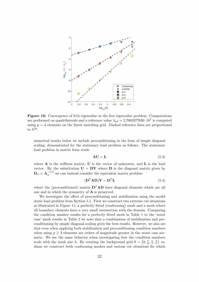
In Figure 9 we give a visual comparison of an eigenmode computed usingp = 2 elements with conforming FEM and CutFEM in two different cut situ-ations and we note no noticeable differences. To investigate the convergencein eigenvalues we as reference use conforming FEM with p = 4 elements on afine grid. The convergence results for an eigenvalue is presented in Figure 10and we see that CutFEM in this problem performs equivalently to conformingFEM.
5.2 Condition Numbers
As the domain is allowed to cut the elements in the background grid in an arbi-trary fashion we may end up with cut situations in which the method becomesill-conditioned unless properly stabilized or preconditioned. While we focus ourwork on the stabilization side an alternative, or complement, to stabilization ispreconditioning techniques which can yield good results, see for example [7]. In the
19

Figure 7: Meshes used in the frequency response calculations.
3 4 5 6 7 8 9
log(ω2)
0
1
2
3
4
5
6
7
E(ω
)
ConformingCutFEM h=0.1
3 4 5 6 7 8 9
log(ω2)
0
1
2
3
4
5
6
7
E(ω
)
ConformingCutFEM h=0.05
Figure 8: Energy in frequency response calculations. p = 2
20

Figure 9: Shape and von-Mises stress for 6:th eigenmode using p = 2 elements. From topto bottom: Conforming FEM, CutFEM with the background mesh rotated θ = π/9 respec-tively θ = π/4. There are no visible differences in the shape and only minute differences inthe stress.
21
-2 -1.8 -1.6 -1.4 -1.2 -1 -0.8 -0.6 -0.4
log10
(h)
-12
-10
-8
-6
-4
-2
0
log
10 | λ
- λ
h |
ConformingCutFEMp=1p=2p=3
Figure 10: Convergence of 6:th eigenvalue in the free eigenvalue problem. Computationsare performed on quadrilaterals and a reference value λref = 2.7063377630 ·107 is computedusing p = 4 elements on the finest matching grid. Dashed reference lines are proportionalto h2p.
numerical results below we include preconditioning in the form of simple diagonalscaling, demonstrated for the stationary load problem as follows. The stationaryload problem in matrix form reads
AU = L (5.3)
where A is the stiffness matrix, U is the vector of unknowns, and L is the loadvector. By the substitution U = DY where D is the diagonal matrix given by
Dii = A−1/2ii we can instead consider the equivalent matrix problem
(DTAD)Y = DTL (5.4)
where the (proconditioned) matrix DTAD have diagonal elements which are allone and in which the symmetry of A is preserved.
We investigate the effect of preconditioning and stabilization using the modelstatic load problem from Section 5.1. First we construct two extreme cut situationsas illustrated in Figure 11; a perfectly fitted (conforming) mesh and a mesh whereall boundary elements have a very small intersection with the domain. Comparingthe condition number results for a perfectly fitted mesh in Table 1 to the ‘worstcase’ mesh results in Table 2 we note that a combination of stabilization and pre-conditioning by simple diagonal scaling gives the best results. However, we also seethat even when applying both stabilization and preconditioning condition numberswhen using p ≥ 3 elements are orders of magnitude greater in the worst case sce-nario. We see the same behavior when investigating how the condition numbersscale with the mesh size h. By rotating the background grid θ = 0, π9 ,
π7 ,
π5 ra-
dians we construct both conforming meshes and various cut situations for which
22

Figure 11: Meshes used in estimation of condition numbers. Perfectly fitted mesh (left)and a ‘worst case’ mesh (right) where only 1/1000 of the boundary elements are inside thedomain.
Table 1: Numerical condition number estimates for stiffness matrix A and mass matrix Min the perfectly fitted situation in Figure 11. The preconditioning here is a simple diagonalscaling of the matrix.
A p Plain Precond. M p Plain Precond.
1 5.2187 · 105 3.4096 · 103 1 2.2392 · 101 1.1646 · 101
2 5.0805 · 106 2.7717 · 104 2 6.1285 · 101 1.3824 · 101
3 1.9148 · 107 1.1609 · 105 3 1.2169 · 102 2.0935 · 101
4 6.0930 · 107 4.6446 · 105 4 3.1309 · 102 3.4586 · 101
5 1.7828 · 108 1.7832 · 106 5 9.6345 · 102 6.2514 · 101
we compare condition numbers from preconditioning by diagonal scaling alone tocondition numbers when we also add stabilization, i.e. CutFEM. In Figure 12 wefor p = 1, 2 elements see good results, both regarding scaling and size of condi-tion numbers. Note that for p = 1 elements preconditioning by diagonal scalingalone is sufficient. For p = 3, 4, 5 elements we in Figure 13 see that the conditionnumbers scale in the correct manner but their size in cut situations are orders ofmagnitude higher compared to those of conforming FEM. Reviewing the analyticalresults above we attribute this effect to the constant in the inverse estimates (4.9),(4.16) and (4.23) which can become quite large for higher order polynomials.
5.3 Thin Geometries
It is well known that low order elements (p = 1) in elasticity problems suffer fromlocking on thin geometries when the number of elements in the thickness directionapproaches one. This effect stems from the boundary condition σ(u) ·n = 0 whichin such situations constrains the non-zero components of the stress to the tangentialplane. In CutFEM the situation may become even more extreme as the number
23

Table 2: Numerical condition number estimates for the stiffness matrix A and the massmatrix M for the ‘worst case’ cut situation in Figure 11 where only 1/1000 of boundaryelements are inside the domain. The preconditioning here is a simple diagonal scaling ofthe matrix.
A p Plain Precond. Stabilized Stab. + Precond.
1 1.6675 · 1016 2.8270 · 103 4.6725 · 106 2.9021 · 103
2 6.0692 · 1030 1.4264 · 1016 1.0239 · 109 2.3952 · 104
3 1.6325 · 1032 4.0341 · 1019 1.3580 · 1011 4.7715 · 105
4 3.0219 · 1032 1.0862 · 1020 2.2118 · 1013 1.1224 · 108
5 4.1334 · 1033 2.0851 · 1021 4.4914 · 1015 3.5444 · 1010
M p Plain Precond. Stabilized Stab. + Precond.
1 2.6963 · 1019 1.1848 · 101 3.4553 · 103 1.5677 · 101
2 3.8825 · 1034 5.1576 · 1016 1.8307 · 105 1.3623 · 103
3 1.2091 · 1035 5.7858 · 1018 1.0203 · 107 2.6414 · 105
4 3.6643 · 1035 6.0559 · 1019 1.4240 · 109 6.7336 · 107
5 4.7194 · 1035 5.1345 · 1019 5.3499 · 1011 2.4344 · 1010
-2 -1.8 -1.6 -1.4 -1.2 -1
log(h)
2
4
6
8
10
12
14
16
18
log(
cond
(A))
ConformingCutFEMUnstabilizedp=1p=2
-2 -1.8 -1.6 -1.4 -1.2 -1
log(h)
0
2
4
6
8
10
12
14
16
18
log(
cond
(M))
ConformingCutFEMUnstabilizedp=1p=2
Figure 12: Numerical estimation of condition numbers for the stiffness matrix (left) andthe mass matrix (right) using p = 1, 2 elements. All results includes preconditioningby simple diagonal scaling. The dashed reference lines indicate the theoretical conditionnumber scaling of h−2 for the stiffness matrix and constant scaling for the mass matrix.
24

-2 -1.8 -1.6 -1.4 -1.2 -1
log(h)
4
6
8
10
12
14
16
18
20
22
log(
cond
(A))
ConformingCutFEMUnstabilizedp=3p=4p=5
-2 -1.8 -1.6 -1.4 -1.2 -1
log(h)
0
2
4
6
8
10
12
14
16
18
20
log(
cond
(M))
ConformingCutFEMUnstabilizedp=3p=4p=5
Figure 13: Numerical estimation of condition numbers for the stiffness matrix (left) andthe mass matrix (right) using p = 3, 4, 5 elements. All results includes preconditioningby simple diagonal scaling. The dashed reference lines indicate the theoretical conditionnumber scaling of h−2 for the stiffness matrix and constant scaling for the mass matrix.
of elements in the thickness direction can be a small fraction of an element. Thiseffect is illustrated in Figure 14 where a thin cantilever beam under gravitationalload using large elements exhibits extreme locking when using p = 1 elements whilethere is no such effects when using higher order elements.
Furthermore, in CutFEM it is possible for the geometry to be curved inside anelement, yielding a tangential plane with non-zero curvature. To avoid locking insuch situations when using coarse meshes we must use even higher order elementsor increase resolution until the curvature is small compared to the element size.As an illustration of this we here consider a free ring under a centrifugal load.In Figure 15 we note that while p = 2 elements yield fairly good results for thismesh resolution we need p = 3 elements for visually perfect results with regards torotational symmetry for the stress distribution.
5.4 Compound Bodies
Compound bodies consist of several subdomains where the discrete solution on eachsubdomain is described on a separate mesh. Such a construction gives a number ofpowerful modeling possibilities, for example
• adding or changing small geometric details, for example fillets, without need-ing to reassemble all matrices
• in each subdomain using different material properties, mesh resolution or el-ements
25

Figure 14: Thin cantilever beam under gravitational loading. Von Mises stresses in athin cantilever beam under gravitational load using p = 1, 2, 3 elements. Note the extremelocking occuring when using p = 1.
0 1 2 3 4 5 6-8
-6
-4
-2
0
2
4
6
%
0 1 2 3 4 5 6-0.06
-0.04
-0.02
0
0.02
0.04
%
0 1 2 3 4 5 6-1.5
-1
-0.5
0
0.5
1
%
×10-3
Figure 15: Ring under centrifugal load. Top: Von Mises stresses for p = 1, 2, 3 elements.Bottom: Variation in midline radial displacement relative to its mean.
26

Ω1 Ω2
Γ12
n
Figure 16: Illustration of compound body consisting of two subdomains Ω1 and Ω2 joinedat the interface Γ12 = ∂Ω1 ∩ ∂Ω2 with prescribed normal n = n∂Ω1 .
• constructing objects from a number of predefined and preassembled buildingblocks
The weak enforcement of Dirichlet boundary conditions by Nitsche’s method [19]in CutFEM makes it easy to construct compound bodies by a simple adaptation ofNitsche’s method to interface conditions.
Consider the schematic compound body illustrated in Figure 16 for which wehave the following interface conditions on Γ12
[u] = 0 on Γ12 (5.5a)
[σ(u) · n] = 0 on Γ12 (5.5b)
Summing the standard CutFEM formulations for all subdomains, with discretefunctions on each subdomain described on its own background grid (and possiblyits own type of elements), we for this example have the following interface term
I12 = −(σ(u) · n∂Ω1 ,v)∂Ω1∩Γ12 − (σ(u) · n∂Ω2 ,v)∂Ω2∩Γ12 (5.6)
From this term and the interface conditions (5.5) we derive Nitsche’s method forthe interface conditions via the calculation
I12 = −(σ(u) · n,v)∂Ω1∩Γ12 + (σ(u) · n,v)∂Ω2∩Γ12 (5.7)
= −(σ(u) · n− [σ(u) · n]/2︸ ︷︷ ︸=0 by (5.5b)
,v)∂Ω1∩Γ12 + (σ(u) · n− [σ(u) · n]/2︸ ︷︷ ︸=0 by (5.5b)
,v)∂Ω2∩Γ12
(5.8)
= −(σ(u) · n− [σ(u) · n]/2︸ ︷︷ ︸=〈σ(u)·n〉
, [v])Γ12 (5.9)
= −(〈σ(u) · n〉, [v])Γ12 − ([u], 〈σ(v) · n〉)Γ12 + γDh−1([u], [v])Γ12︸ ︷︷ ︸
=0 by (5.5a)
(5.10)
As an illustration of compound bodies we in Figures 17 and 18 consider an L-shape domain where the inside corner has been drilled to avoid a stress singularity inthe solution. We have constructed this domain out of three subdomains describedon three different background grids and we use p = 2 elements to represent thesolution on each mesh. Note that there is no need for the various meshes to matchat the interface as the interface conditions are enforced weakly.
27

Figure 17: Detail of drilled aluminium L-shape constructed as 3 separate bodies. Notethe perfect flow of the von-Mises stress over the interfaces.
Figure 18: Detail of drilled L-shape constructed as 3 separate bodies. Inner ring issteel, outer part of domain has 1/10 the stiffness of steel. Inner ring mesh also has higherresolution. Note the distinct discontinuity of the von-Mises stress over the interface whichis due to the discontinuity of material stiffness.
28

5.5 Two-Grid Eigenvalue Estimation
The use of structured background grids in CutFEM is very convenient when em-ploying multi-grid techniques. We here illustrate this with a two-grid method forestimation of eigenvalues [25]. Consider two background grids, one coarse grid withmesh size H and one fine with mesh size h, constructed such that the fine grid is arefinement of the coarse grid. The two-grid algorithm reads
1. Solve the eigenvalue problem on the coarse background grid: Find (uH , λH) ∈VH × R such that
AH(uH ,v)− λHmH(uH ,v) = 0 , ∀v ∈ VH (5.11)
2. Solve a single linear problem on the fine background grid: Find uh ∈ Vh
Ah(uh,v) = λHmh(uH ,v) , ∀v ∈ Vh (5.12)
3. Compute the Rayleigh quotient
λh =‖uh‖ah‖uh‖mh
(5.13)
The analysis in [25] for a conforming two-grid method implies that the optimalchoice of mesh size H for the coarse grid is given by the relationship
H ∝√h (5.14)
However in a cut situation, especially in light of the results in Section 5.3, it is veryreasonable to assume that the coarse grid mesh size must be small enough to givean acceptable approximation of the eigenvalues and eigenmodes for this procedureto be efficient.
As a simple numerical example we consider the eigenvalue problem of a freering with coarse and fine grids illustrated in Figure 19. As this is a free eigenvalueproblem we in step 2 of the algorithm must seek the solution uh ∈ Vh/RM . Theresulting approximations of the 10:th eigenvalue and the corresponding eigenmodeare presented in Figure 20 together with a reference solution computed using highorder parametric conforming FEM.
6 Modeling of Embedded Structures with Ap-
plication to Fibre Reinforced Materials
In this Section we consider the embedding of membranes, thin plates, truss andbeam elements into a higher dimensional elastic body. Simulations of this type aresuitable for reinforced structures, e.g., reinforced concrete, fiber reinforced poly-mers, and composite materials in general.
The approach is based on:
29

Figure 19: Meshes used in two-grid estimation of the 10:th eigenvalue in the free eigenvalueproblem for a steel ring. Here mesh sizes H = 0.1 and h = H/3 are used for the coarse andfine scale meshes, respectively.
Figure 20: Eigenmodes associated with the 10:th eigenvalue computed using CutFEM ona coarse grid (left), CutFEM two-grid estimation on a subgrid (middle), and parametricconforming FEM (right). CutFEM solutions are computed using p = 2 elements while thereference FEM solution is computed using p = 4 elements. Corresponding eigenvalues areλH = 9.99836561 · 106, λh = 9.89445550 · 106, and λref = 9.891710308 · 106. Note that dueto the rotational symmetry of the problem, the rotation of the eigenmode is undetermined.
30

• Given a continuous finite element space, based on at least second second orderpolynomials, we define the finite element space for the thin structure as therestriction of the bulk finite element space to the thin structure which isgeometrically modeled by an embedded curve or surface.
• To formulate a finite element method on the restricted or trace finite elementspace we employ continuous/discontinuous Galerkin approximations of plateand beam models.
The thin structures are then modelled using the CutFEM paradigm and the stiffnessof the embedded structure is in the most basic version, which we consider here,simply added to the bulk stiffness. This in turn means that the bulk stabilizesthe CutFEM contributions and no additional stabilization is needed. In this initialreport, we limit ourselves to two-dimensional bulk problems and thus the embeddedstructures will be limited to trusses and beams. In future work, the handling ofKirchhoff plates and beams and trusses of codimension 2 will be considered. Thebulk problem may also be viewed as an interface problem on the case of an embeddedsurface in three dimensions or curve in two dimensions in order to more accuratelyapproximate the bulk problem in the vicinity of the thin structure.
The work presented here is and extension of earlier work [6] where only mem-brane structures were considered, in which case a linear approximation in the bulksuffices.
6.1 Modeling of Trusses and Beams
Consider the elasticity equations (2.1) in Ω ⊂ R2. Embedded in Ω we have straighttruss and beam elements. Curved elements can be modeled using piecewise affineapproximations of the curve, following [14].
We consider modeling the truss and beam using tangential differential calcu-lus. To this end we follow the exposition in [15] and then make some simplifyingassumptions. Let then Σ denote line embedded in R2, with tangent vector t. Welet p : R2 → Σ be the closest point mapping, i.e. p(x) = y where y ∈ Σ mini-mizes the Euclidean norm |x − y|R3 . We define ζ as the signed distance functionζ(x) := ±|x− p(x)|, positive on one side of Σ and negative on the other. The lineΣ is assumed to be the center line of a truss element with thickness t, which we forsimplicity assume is constant.
The linear projector PΣ = PΣ(x), onto the tangent line of Σ at x ∈ Σ, is givenby
PΣ = t⊗ t. (6.1)
Based on the assumption that planar cross sections orthogonal to the midlineremain plane after deformation we assume that the displacement takes the form
u = u0 + θζt (6.2)
where u0 : Σ→ R2 is the deformation of the midline, decomposed as
u0 = unn+ utt, un := u0 · n, ut := u0 · t, (6.3)
31

where n ⊥ t, and θ : Σ → R is an angle representing an infinitesimal rotation.Both u0 and θ are assumed constant in the normal plane.
In Euler–Bernoulli beam theory the beam cross-section is assumed plane andorthogonal to the beam midline after deformation and no shear deformations occur.This means that we have
θ = t · ∇un := ∂tun (6.4)
This definition for θ in combination with (6.2) constitutes the Euler–Bernoulli kine-matic assumption.
We assume the usual Hooke’s law for one dimensional structural members
σΣ(u) = EεΣ(u) (6.5)
where εΣ(u) := PΣε(u)PΣ. We then notice that the strain energy density can bewritten
EεΣ(u) : εΣ(u) = E(t · ε(u) · t)2 = E((∂tut)
2 + ζ2(∂tθ)2). (6.6)
Assuming computations are being done per unit length in the third dimension, thesecond moment of inertia I = t3/12 and the area A = t and the total energy of thetruss and beam structures are postulated as
E = ET + EB (6.7)
where the truss energy
ET :=1
2
∫ΣEA (∂tut)
2 dΣ−∫
ΣAf · tut dΣ (6.8)
and the beam energy
EB :=1
2
∫ΣEI
(∂2ttun
)2dΣ−
∫ΣAf · nun dΣ (6.9)
where ∂2tt := ∂t∂t. Assuming zero displacements and rotations at the end points of
Σ, we thus seek (ut, un) ∈ H10 (Σ)×H2
0 (Σ) such that∫ΣEA∂tut∂tvt dΣ +
∫ΣEI ∂2
ttun∂2ttvn dΣ =
∫ΣA(ftvt + fnvn) dΣ (6.10)
for all (vt, vn) ∈ H10 (Σ)×H2
0 (Σ).
6.2 Finite Element Discretization
In analogy with the preceding discussion, we now let Kh be a quasiuniform partition,with mesh parameter h, of the bulk domain Ω into shape regular elements K, anddenote the set of faces in Kh by Fh. The elements of the bulk mesh cut by Σ, andthe corresponding element faces, are denoted
Kh(Σ) = K ∈ Kh : K ∩ Γ 6= ∅ (6.11)
Fh(Σ) = F ∈ Fh : F ∩ ∂K 6= ∅ , K ∈ Kh(Σ) (6.12)
32

The intersection points between Σ and element faces in Kh(Σ) is denoted
Ph(Σ) = x : x = F ∩ Σ, F ∈ Fh, (6.13)
and we assume that this is a discrete set of points (thus excluding the case whereany F ∈ Fh coincides with a part of Σ of nonzero measure). Setting as above
a(v,w) := 2µ(ε(v), ε(w))Ω + λ(tr(ε(v)), tr(ε(w)))Ω (6.14)
and introducingb(v,w) := (EA∂t(v · t), ∂t(w · t))Σ (6.15)
andc(v,w) := (EI ∂2
tt(v · n), ∂2tt(w · n))Σ (6.16)
and defining atot(v,w) := a(v,w) + b(v,w) + c(v,w) we propose the followingcontinuous/discontinuous Galerkin method. With
Vh := v : v|K ∈ [P 2(K)]2 ∀K ∈ Kh, v ∈ [C0(Ω)]2, v = 0 on ∂Ω (6.17)
we seek u ∈ Vh such that
(Af ,v)Σ + (f ,v)Ω = atot(u,v)−∑
x∈Ph(Σ)
〈EI∂2tt(u(x) · n)〉[∂t(v(x) · n)]
−∑
x∈Ph(Σ)
〈EI∂2tt(v(x) · n)〉[∂t(u(x) · n)]
+∑
x∈Ph(Σ)
βEI
h[∂t(u(x) · n)][∂t(v(x) · n)] (6.18)
for all v ∈ Vh. Here
〈f(x)〉 :=1
2(f(x+ εt) + f(x− εt)) |ε↓0, [f(x)] := (f(x+ εt)− f(x− εt)) |ε↓0.
(6.19)The terms on the discrete set Ph(Σ) are associated with the work of the end mo-ments on the end rotation which occur due to the lack of C1(Ω) continuity of theapproximation, cf. [14]. In this formulation, stabilization terms of the kind dis-cussed above can be added to ensure coercivity. Due to the presence of the bulkequations, the need for these terms is however mitigiated.
6.3 Numerical Examples
We consider a bulk material on the domain Ω = (0, 4)×(0, 1) with E = 300, ν = 1/3in plane strain. The domain is fixed at the left end and unloaded on the rest of theboundary. It is first loaded with a volume load f = (0,−1) and the displacementsusing only the bulk material are shown in Fig. 21 with corresponding (Frobenius)norm of the stresses shown in Fig. 22. We next introduce two truss elements asshown in Fig 23 at y = 0.249 and at y = 0.751. The thickness of the trusseswas set to t = 0.1 and Young’s modulus E = 104. In Figs. 24 and 25 we show
33

0 0.5 1 1.5 2 2.5 3 3.5 4
-1.5
-1
-0.5
0
0.5
1
1.5
Figure 21: Deformation of the bulk material.
the corresponding deformations and norm of the stresses. Finally we remove thetrusses and add a beam at y = 0.501, with thickness t = 0.1 and E = 106. In Figs.26 and 27 we show the corresponding deformations and norm of the stresses.
In our second example we use the same boundary conditions but pull the ma-terial using f = (100, 0). The corresponding displacements using only the bulkmaterial are shown in Fig. 28 with associated norm of the stresses shown in Fig.29. We then insert the truss elements from the previous example and apply theload again to obtain the deformation shown in Fig. 30 with associated norm ofstresses in Fig. 31.
In all these examples we see that the added lower dimensional structural ele-ments have a profound impact on the deformation and stress distribution in thebulk material. The possibility of modeling lower dimensional structural elementswithout meshing is clearly beneficial and can be used for example in optimizationalgorithms where the structural members are required to move around to find theiroptimal shape and place.
34

0
20
0
40
60
80
100
21
0.80.6
0.40.24 0
Figure 22: Norm of the stresses in the bulk.
0.5 1 1.5 2 2.5 3 3.5 4
-1
-0.5
0
0.5
1
1.5
2
Figure 23: Trusses in the bulk.
35

0 1 2 3 4
-1
-0.5
0
0.5
1
1.5
Figure 24: Deformation with trusses.
0
0
10
20
30
1
40
50
2
60
10.83 0.6
0.40.24 0
Figure 25: Norm of the stresses with trusses.
36

0 0.5 1 1.5 2 2.5 3 3.5 4
-1
-0.5
0
0.5
1
1.5
Figure 26: Deformation with beam.
0
0
1
10
2
10.8
3 0.6
20
0.40.2
40
30
Figure 27: Norm of the stresses with beam.
37

0 1 2 3 4 5 6
-1
0
1
2
3
Figure 28: Deformation of pulled bulk material.
100.5
1000
800
600
0
400
200
0
2 4
Figure 29: Norm of the stresses; pulled bulk material.
38

0 0.5 1 1.5 2 2.5 3 3.5 4
-1
-0.5
0
0.5
1
1.5
2
Figure 30: Deformation of pulled bulk material with trusses.
0
50
100
150
0
200
2 10.5
40
Figure 31: Norm of the stresses; pulled bulk material with trusses.
39

References
[1] R. Becker, E. Burman, and P. Hansbo. A Nitsche extended finite elementmethod for incompressible elasticity with discontinuous modulus of elasticity.Comput. Methods Appl. Mech. Engrg., 198(41-44):3352–3360, 2009.
[2] S. C. Brenner and L. R. Scott. The mathematical theory of finite elementmethods, volume 15 of Texts in Applied Mathematics. Springer, New York,third edition, 2008.
[3] E. Burman, S. Claus, P. Hansbo, M. G. Larson, and A. Massing. Cutfem:Discretizing geometry and partial differential equations. Internat. J. Numer.Methods Engrg., 2015.
[4] E. Burman and P. Hansbo. Fictitious domain finite element methods usingcut elements: I. A stabilized Lagrange multiplier method. Comput. MethodsAppl. Mech. Engrg., 199(41-44):2680–2686, 2010.
[5] E. Burman and P. Hansbo. Fictitious domain finite element methods using cutelements: II. A stabilized Nitsche method. Appl. Numer. Math., 62(4):328–341,2012.
[6] M. Cenanovic, P. Hansbo, and M. G. Larson. Cut finite element modeling oflinear membranes. Comput. Methods Appl. Mech. Engrg., 310:98–111, 2016.
[7] F. de Prenter, C. V. Verhoosel, G. J. van Zwieten, and E. H. van Brumme-len. Condition number analysis and preconditioning of the finite cell method.Comput. Methods Appl. Mech. Engrg., 316:297–327, 2017.
[8] A. Ern and J.-L. Guermond. Evaluation of the condition number in linear sys-tems arising in finite element approximations. ESAIM: Math. Model. Numer.Anal., 40(1):29–48, 2006.
[9] T.-P. Fries and S. Omerovic. Higher-order accurate integration of implicitgeometries. Internat. J. Numer. Methods Engrg., 106(5):323–371, 2016.
[10] T. P. Fries, S. Omerovic, D. Schollhammer, and J. Steidl. Higher-order meshingof implicit geometries—Part I: Integration and interpolation in cut elements.Comput. Methods Appl. Mech. Engrg., 313:759–784, 2017.
[11] J. Grande and A. Reusken. A higher order finite element method for partialdifferential equations on surfaces. SIAM J. Numer. Anal., 54(1):388–414, 2016.
[12] S. Gross, M. A. Olshanskii, and A. Reusken. A trace finite element method fora class of coupled bulk-interface transport problems. ESAIM: Math. Model.Numer. Anal., 49(5):1303–1330, 2015.
[13] A. Hansbo, P. Hansbo, and M. G. Larson. A finite element method on com-posite grids based on Nitsche’s method. ESAIM: Math. Model. Numer. Anal.,37(3):495–514, 2003.
[14] P. Hansbo and M. G. Larson. Continuous/discontinuous finite element mod-elling of Kirchhoff plate structures in R3 using tangential differential calculus.ArXiv e-prints, abs/1702.03662, 2017.
40

[15] P. Hansbo, M. G. Larson, and K. Larsson. Variational formulation of curvedbeams in global coordinates. Comput. Mech., 53(4):611–623, 2014.
[16] T. Jonsson, M. G. Larson, and K. Larsson. Cut finite element methods on mul-tipatch parametric surfaces. Technical report, Umea University, Dept. Math-ematics and Mathematical Statistics, 2017.
[17] M. G. Larson and F. Bengzon. The finite element method: theory, implemen-tation, and applications, volume 10 of Texts in Computational Science andEngineering. Springer, Heidelberg, 2013.
[18] A. Massing, M. G. Larson, A. Logg, and M. E. Rognes. A stabilized Nitschefictitious domain method for the Stokes problem. J. Sci. Comput., 61(3):604–628, 2014.
[19] J. A. Nitsche. Uber ein Variationsprinzip zur Losung von Dirichlet-Problemenbei Verwendung von Teilraumen, die keinen Randbedingungen unterworfensind. Abh. Math. Univ. Hamburg, 36:9–15, 1971.
[20] M. A. Olshanskii, A. Reusken, and J. Grande. A finite element method forelliptic equations on surfaces. SIAM J. Numer. Anal., 47(5):3339–3358, 2009.
[21] M. A. Olshanskii, A. Reusken, and X. Xu. On surface meshes induced by levelset functions. Comput. Vis. Sci., 15(2):53–60, 2012.
[22] J. Parvizian, A. Duster, and E. Rank. Finite cell method: h- and p-extensionfor embedded domain problems in solid mechanics. Comput. Mech., 41(1):121–133, 2007.
[23] M. Ruess, D. Schillinger, Y. Bazilevs, V. Varduhn, and E. Rank. Weaklyenforced essential boundary conditions for NURBS-embedded and trimmedNURBS geometries on the basis of the finite cell method. Internat. J. Numer.Methods Engrg., 95(10):811–846, 2013.
[24] D. Schillinger and M. Ruess. The finite cell method: a review in the contextof higher-order structural analysis of CAD and image-based geometric models.Arch. Comput. Methods Eng., 22(3):391–455, 2015.
[25] J. Xu and A. Zhou. A two-grid discretization scheme for eigenvalue problems.Math. Comp., 70(233):17–25, 2001.
41