On finite-difference solutions in elasticity

Item Type text; Thesis-Reproduction (electronic)

Authors Fangmann, Robert Edward, 1943-

Publisher The University of Arizona.

Rights Copyright © is held by the author. Digital access to this materialis made possible by the University Libraries, University of Arizona.Further transmission, reproduction or presentation (such aspublic display or performance) of protected items is prohibitedexcept with permission of the author.

Download date 19/07/2018 05:01:38

Link to Item http://hdl.handle.net/10150/318618

ON FINITE-DIFFERENCE SOLUTIONS IN ELASTICITY

byRobert Edward Fangmann

A Thesis Submitted to the Faculty of the

DEPARTMENT OF CIVIL. ENGINEERING

In Partial Fulfillment of the'Requirements For the Degree of

MASTER OF SCIENCE

In the Graduate College

THE UNIVERSITY OF ARIZONA

1 9 6 7

STATEMENT BY AUTHOR

This thesis has been submitted in partial fulfill­ment of requirements for an advanced degree at the University of Arizona and is deposited in the University Library to be made available to borrowers under rules of the Library.

Brief quotations from this thesis are allowable without special permission, provided that accurate acknowledgment of source is made. Requests for permission for extended quotation from or reproduction of this manuscript in whole or in part may be granted by the head of the major department or the Dean of the Graduate College when in his judgment the proposed use of the material is in the interests of scholarship.In all other instances, however, permission must be obtained from the author.

This thesis has been approved on the date shown below:

SIGNED: A

APPROVAL BY THESIS DIRECTOR

7 RICHMOND C. ^ipF Professor of Civil Engineering

Y u £ 7uDate '

ACKNOWLEDGMENTS

The author wishes to express his sincere thanks

to his major advisor, Dr. Richmond C. Neff, for his

encouragement, guidance, and technical assistance during

the preparation of this thesis.

The author also wishes to express his thanks to

his wife, Bonnie, for her assistance in preparing his

manuscript,

TABLE OF CONTENTS

PageLIST OF ILLUSTRATIONS........... . vi

LIST OF T A B L E S ................... vii

LIST OF SYMBOLS. . . ..... . . . . . . . . . . .viii

ABSTRACT............... ................... .. ix

CHAPTER

I INTRODUCTION. . . . . . . . . . . . . . . . . 1

II DERIVATION OF THE WORKING EQUATIONS . . . . . 8

Derivation of Navier *s Equations, . . . . . 8Navier's Equations for Plane Stress . . . . 9Navier's Equations for Plane Strain . . . . 11Boundary Conditions . . . . . . . . . . . . 12Summary . . . . . . . . . . . . . . . . . . 12

III FINITE-DIFFERENCE REPRESENTATION OF THEWORKING EQUATIONS . ...................... . 14

Navier’s Equations. . . . . . . . . . . . . 16Boundary Conditions . . . . . . . . . . . . 18Transition Points . . . . . . . . . . . . . 20Summary . . . . . . . . . . . . . . . .. . . 23Stress-Strain Equations . . . . . . . . . . 25Graded Mesh . . . . . . . . . . ............ 26

IV METHODS OF SOLUTION . . . ........... 30

Numerical Solution, . . . . . . . . . . . . 30Photoelastic Solution . . . . . . . . . . . 34

V RESULTS AND CONCLUSIONS . . . . . . . . . . . 38

Accuracy of Numerical Solutions . . . . . . 38Photoelastic Solution as a Measure ofthe Accuracy of the Numerical Solutions . . 42Conclusions . . . . . m . . . . . . . . . . 44Proposal for Future Investigation . . . . . 45

iv

V

TABLE OF CONTENTS--Continued

Page

APPENDIX. . . . . . . . . . . . . . . . . . . . . . 47

REFERENCES. . . . . . . . . . . . . . . . . . . . . 51

LIST OF ILLUSTRATIONS

Figure

1

23

4

5

6

7

Clamped Plate with Concentrated Loads. . .

Indexing Procedure for Nodal Points. . . .

Coarse Mesh Superimposed on One Quarter of the Clamped Plate . . . . . . . . . . .

Graded Mesh Superimposed on One Quarter of the Clamped Plate . . . . . . . . . . .

Photograph of Photoelastic Model Showing Isochromatic Fringes for an Applied Load of 405 Pounds. . . . . . . . . . .........

Maximum Shear Stress as a Function of Position from the Load Point to the Middle of the Plate . . . . . . . . . . . . . . .

Maximum Shear Stress as a Function of Position from the Middle of the Plate to the Clamped Edge. . . . . . . . . . . . .

Page

15

17

22

28

36

39

40

vi

Table

1

LIST OF TABLES

Page

Convergence Rates for NumericalSolutions. . . . . . . . . . . . . . . . . . 33

vii

LIST OF SYMBOLS

4V Biharmonic operator.

5 Kronecker Delta.

E Young’s Modulus,

e s t r a i n tensor.

F body force.

h mesh spacing.

K dominant eigenvalue of the iteration matrix.

L length of the edge of the plate.

P applied load,

s Poisson’s Ratio.

stress tensor.

v,X Lame’s constants.

U Airy's Stress Function.

u horizontal displacement or displacement in theXj direction.

v vertical displacement or displacement in thex2 direction.

displacement vector.

viii

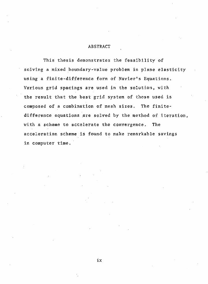
ABSTRACT

This thesis demonstrates the feasibility of

solving a mixed boundary-value problem in plane elasticity using a finite-difference form of Navier1s Equations. Various grid spacings are used in the solution, with the result that the best grid system of those used is

composed of a combination of mesh sizes. The finite- difference equations are solved by the method of iteration, with a scheme to accelerate the convergence. The

acceleration scheme is found to make remarkable savings

in computer time.

CHAPTER I INTRODUCTION

Elasticity is the study of the response of an

elastic material under various loads. An elastic material

is one which deforms under load but returns to its original

shape when the load is removed. Many solid materials

exhibit elastic behavior over some range of loading.

In developing a mathematical theory of elasticity,

elastic materials are usually assumed to be homogeneous

and isotropic. These have been shown to be good assump­

tions. As Sokolnikoff (1956, p. 65) mentions.

Most structural materials are formed of crystalline substances, and hence very small portions of such materials cannot be regarded as being isotropic. Nevertheless, the assump­tion of isotropy and homogeneity, when applied to an entire body, often does not lead to serious discrepancies between the experimental and theoretical results. The reason for this agreement lies in the fact that the dimensions of most crystals are so small in comparison with the dimensions of the body and they are so chaotically distributed that, in the large, the substance behaves as though it were isotropic.

Another assumption which is commonly made in

elasticity is linearity, both geometric arid material.

The assumption of geometric linearity is satisfied if the

derivatives of the displacements in the material are small

enough to neglect products of these terms in comparison to

1

the terms themselves. Material linearity is satisfied if.

the material has a linear relationship between stress and strain in the elastic range. This has also been shown to

be a good assumption for many engineering materials.

The system of governing equations in elasticity

includes the equations of equilibrium» the stress-strain

equationsand the compatibility equations. Also,

equilibrium conditions must be satisfied at the boundary.

This gives rise to boundary conditions which must be met.

Boundary conditions may be in terms of surface

tractions or displacements. Both Boresi (1965) and

Sokolnikoff (1956) list two fundamental types of boundary-

value problems of elasticity. As presented by Sokolnikoff

(1956, p. 73) these are:

Problem 1. Determine the distribution of stress and the displacements in the interior of and elastic body in equilibrium when the body forces are prescribed and the distribution of the forces acting on the surface of the body is known.

Problem 2. Determine the distribution of stress and the displacements in the interior of an elastic body in equilibrium when the body forces are prescribed and the displacements of the points on the surface of the body are prescribed functions.

There is a third type, usually called the Mixed Boundary-Value Problem, which is a combination of these two:

Determine the distribution, of stress and displacements in

the interior,of an elastic body in equilibrium when the

body forces are prescribed and the displacements of the

points on part of the surface of the body are prescribed

function and the distribution of the forces acting on the

remaining part of the surface of the body is known. This

mixed boundary-value problem is the one with which this

thesis is concerned.

Frequently it is difficult to express the boundary

conditions in a convenient mathematical form. Often it is

possible to modify the boundary conditions slightly and

obtain an approximate solution. The modifications must be

in accordance with Saint Venant’s Principle which, as

stated by Sokolnikoff (1956, p. 90), is.

If some distribution of forces acting on a portion of the surface of a body is replaced by a different distribution of forces acting on the same portion of the body, then the effects of the two different distributions on the parts of the body sufficiently far removed from the region of application of the forces are essentially the same, provided that the two distributions of forces are statically equivalent.

This principle is of great practical importance. As an

example, a point load is difficult to express in any

convenient mathematical form, whereas it is relatively

simple to treat it as a distributed load over a small

area of the boundary.

There is a Uniqueness Theorem associated with

linear elasticity which states that there is only one

solution with satisfies the governing equations equilib-

rium, compatibility, and stress-strain and the boundary

conditions„ A proof of this is presented by Sokolnikoff

(1956, pp. 86-88).

There are three methods of obtaining analytic

solutions to the above boundary-value problems. The

Direct Method is to solve the governing differential

equations directly while satisfying all the boundary

conditions. The Inverse Method involves finding a problem

to fit a proposed solution. The Semi-inverse Method

consists in making some assumptions about part of the

solution while leaving sufficient generality in the

solution to satisfy the governing equations and the

boundary conditions. If a solution is obtained, accord­

ing to the Uniqueness Theorem, it is the only solution.

The work involved in the Direct Method is very

often prohibitive beyond a few almost trivial problems.

The Inverse Method is almost useless if there is a specific

problem to be solved. The Semi-inverse Method, therefore,

is the one most often employed. In most problems, simpli­

fying assumptions can be made as the result of symmetry or

of the experience of the investigator in solving similar

problems. Such freedom is possible due to the existence

of the Uniqueness Theorem.

5

In plane elasticity, the Airy Stress Function may

be employed so that the problem is reduced to a solution

of the biharmonic equation V^U = 0, and where U is Airy's

Stress Function. Of course, boundary conditions must

also be satisfied. Again the Direct, Inverse, or Semi­

inverse Method may be used.

The theory of linear elasticity and the different

methods of solution, which are summarized above, have

existed for one hundred years. However, due to the

complicated nature of elasticity problems, only the

simplest problems have been solved in closed form. Recently

the computer has made it possible to apply numerical

methods to the solution of the differential equations of

elasticity. Griffin and Varga (1963) and Allen (1954)

have shown that this method yields a good approximate

solution.

Numerical analysis is most often applied to the

biharmonic equation. As shown in Salvador! and Baron (1961)

and Allen (1954), this method yields a system of linear

algebraic equations which can be solved for values of

the stress function at a number of points in the body and

on the boundary. From these values, stresses and displace­

ments may be calculated at discrete points in the body and

on the boundary. Griffin and Varga (1963) have demonstrated

the usefulness and flexibility of the method. However, in

order to solve the biharmonic equation for the stress

function, it is necessary to express the boundary condi­

tions in terms of the stress function. Because there is

only an indirect relationship between the stress function

and displacements, it is difficult, if not impossible, to apply this method to the second or to the mixed type of boundary-value problem.

Numerical analysis can also be applied to some

other form of the governing equations. This thesis is

concerned with the numerical solution of Navier's Equations

with mixed boundary conditions, Navier*s Equations relate

displacements and body forces and are derived using the

equilibrium equations, the stress-strain equations, and

the strain-displacement relations. Navier*s Equations

yield displacements from which the stresses can be cal­

culated .

Applying numerical methods to Navier*s Equations

yields a set of linear algebraic equations with displace­

ments as unknowns. To solve this set of equations, an

iterative method with an acceleration scheme due to

Faddeeva (1959) is used. Faddeeva * s acceleration scheme

involves obtaining the dominant eigenvalue of the iteration

matrix and using it to accelerate the convergence of

iteration.

The photoelastic method of obtaining a solution to the same problem is used as a check on the accuracy of the

approximate numerical solution. The photoelastic method

is an experimental method which is subject only to

experimental errors in manufacture and loading of the model,

in measuring of data, and in defects in the optical system.

CHAPTER II

DERIVATION OF THE WORKING EQUATIONS

Derivation of Navier’s Equations

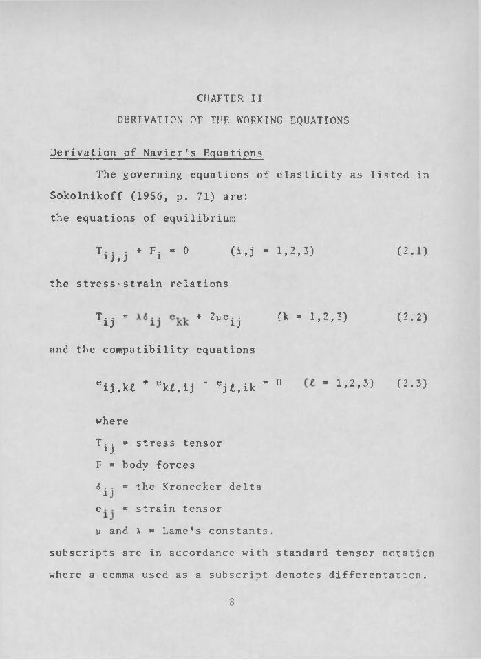
The governing equations of elasticity as listed in

Sokolnikoff (1956, p. 71) are:

the equations of equilibrium

Tij,j * Fi = 0 ( M = 1,2,3) (2.1)

the stress-strain relations

^ij = + 2v g ̂ j (k = 1,2,3) (2.2)

and the compatibility equations

eij,k£ * ekZ,ij ' ejZ,ik “ 0 1>2>3:i f2'3)

where

T^j * stress tensor

F » body forces

6 ̂ j = the Kronecker delta

e = strain tensor

\i and X = Lame's constants,

subscripts are in accordance with standard tensor notation

where a comma used as a subscript denotes differentation.

8

9Differentiating the stress-strain relations,

substituting this into the equations of equilibrium, and

using the strain-displacement relations

where = displacement vector.

Equations (2.5) are Navier's Equations in three dimensions.

Navier's Equations for Plane Stress

For plane stress, we take » T 23 * = 0.

Consider the stress-strain equation for T ^ .

1/2 (w (2.4)

yield

(2.5)

(2.6)

so (2.7)

and "3.3> (a *= 1,2) (2.8)

(2.9)

Substituting for w, , from Equation (2.8) yields

(2.10)

10Now consider the stress-strain equations for plane

stress.

T.S ‘ U(V B + "B,.) + X5aBWk,k ' I'Z) I2'11)

Substituting for ^ from Equation (2.10) yields

Ta8 ° u(Wa.B + "s.J + 7 7 ^ 6a8wr,Y(Y - 1,2) (2.12)

The equilibrium equations for plane stress are

T a B , B + F a " 0 <2 - 1 3 )

Differentiating Equations (2.12) with respect to syields

ToB,B “ u (Wa,BB *W B, aB) + x *a8*Y,YB (:2-14)

Substituting this into the equilibrium equations yields

0 ‘ “ K . B B + W B , a B ) + 7 7 7 ; 5aBW Y,YB + Fa C2 '15)

0 ** tiWa , BB W 8 , Bo F a (2 - 1 6 )

Let C = 2ii.A ♦ 2y

T h e n 0 = W a , B B * C W B , 6 a * f (2 - 1 7 )

Equations (2.17) are Navier’s Equations for plane stress.

11Navier's Equations for Plane Strain

For plane strain, e ^ = 7 = w i 3 ” 0eExpanding Navier's Equations in three dimensions and

imposing the restrictions for plane strain yields

0 “ + C* + WB,Ba * Fa t2-1^

(x + w) w For 0 » w + + — (2.19)

0,136 u vLet C = ~ * - v

V

Tben 0 - wa(BB + C'wB>Ba ♦ -2- (2.20)

Equations (2.20) are Navier's Equations for plane strain.

Summarizing, Navier's Equations for two dimensions

areF

0 G a a * Cw a + — for plane stress (2.21)CIj P p P , p CI jj

Fand 0 = w ao ♦ C'w0 0 + — for plane strain (2.22)a , p p p ,doi p

Since E * — ~ and s ■ --- ----X + u 2 X 2 v

C * -— -— - and C =--— ---- where1 - s 1 - 2s

E = Young's Modulus and s = Poisson's Ratio. Notice

that the two constants which express the material

properties are functions of Poisson's Ratio only.

For the problem proposed in Chapter III, the plane

stress form of Navier’s Equations is used.

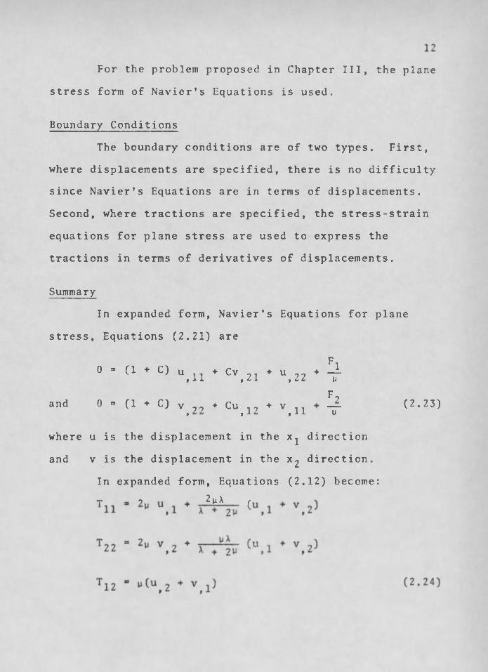
Boundary Conditions

The boundary conditions are of two types. First,

where displacements are specified, there is no difficulty

since Navier's Equations are in terms of displacements.

Second, where tractions are specified, the stress-strain

equations for plane stress are used to express the

tractions in terms of derivatives of displacements.

Summary

In expanded form, Navier’s Equations for plane

stress, Equations (2.21) are

F0 = (1 + C) u + Cv + u + 1

,11 ,21 ,22 T TF?

and 0 = (1 ♦ C) v 77 ♦ Cu 17 ♦ v ^ — (2.23), , l ,ll u

where u is the displacement in the x^ direction

and v is the displacement in the X2 direction.

In expanded form, Equations (2.12) become:~ ~ 2 p X r

13where

I n = normal stress in the %i direction

T22 * normal stress in the %2 direction

T 12 = shear stress.

Equations (2;24) are used to obtain the boundary conditions

at boundary points at which surface tractions are pre­

scribed, and also to obtain the stresses at interior points

when the displacements have been determined.

CHAPTER III

FINITE-DIFFERENCE REPRESENTATION

OF THE WORKING EQUATIONS

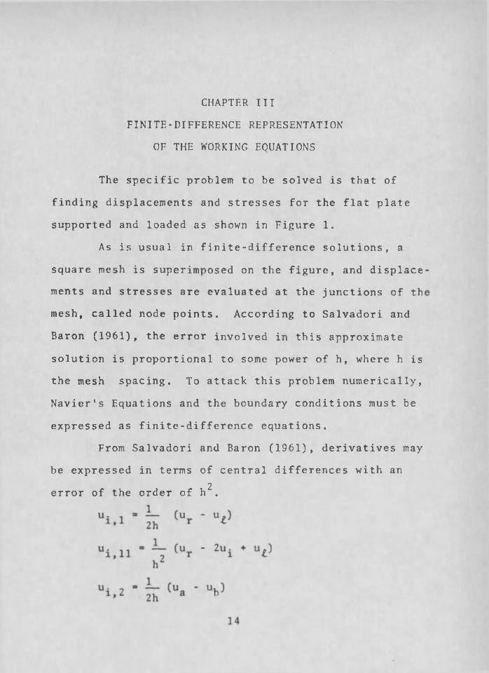
The specific problem to be solved is that of

finding displacements and stresses for the flat plate

supported and loaded as shown in Figure 1.

As is usual in finite-difference solutions, a

square mesh is superimposed on the figure, and displace

ments and stresses are evaluated at the junctions of th

mesh, called node points. According to Salvadori and

Baron (1961), the error involved in this approximate

solution is proportional to some power of h , where h is

the mesh spacing. To attack this problem numerically,

Navier’s Equations and the boundary conditions must be

expressed as finite-difference equations.

From Salvador! and Baron (1961), derivatives may

be expressed in terms of central differences with an2error of the order of h .

15

L/2

Figure 1

Clamped Plate with Concentrated Loads

16

(3.1)

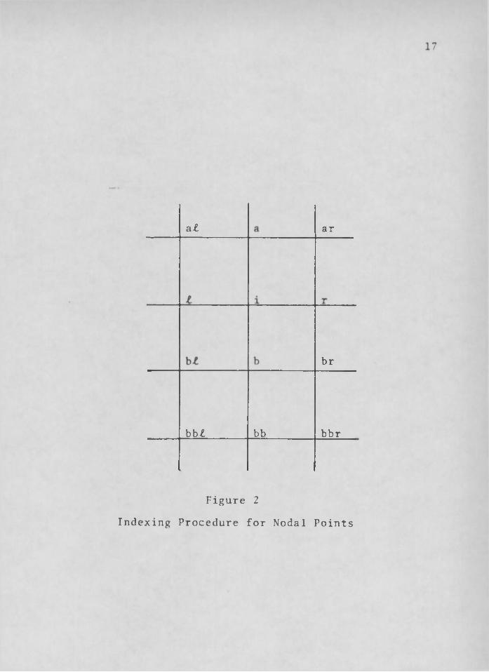
The subscripts r , I , a, and b designate displacements at

points which are either to the right, or left, above, or

evaluated, as shown in Figure 2. The parameter h is the

mesh spacing.

Navier's Equations

Applying Equations (3.1) to Navier's Equations,

Equations (2.23), for plane stress yields

below the i**1 point where the derivative is being

0 = (1 + C) (ur

a£ ar

br

b b l bb bbr

Figure 2

Indexing Procedure for Nodal Points

and 0 = (1 + C) O a - 2vi +vb) ♦ £ (uar - ubr - u18

4 v“ar "br “ at

v 2 C+ "bf) + vr ' 2vi * * 2 (3.2)

Boundary Conditions

Expressing the boundary conditions, Equations

(2.24), as finite-difference equations yields

T 2p A ,122 ' (Ur • + (Va - Vb)

and T 12 =(— ) w (ua ' ub + vr - v£) (3.3)2h

The equation for ̂ is not included since it does not

enter into the proposed problem.

For the proposed problem, the shear stress is

zero on the upper and lower edges. So

T 12 ' 0 ' (̂ }u (ua - ub + vr ' vl>

or 0 « ua - u^ + vr - (3.4)

Where the normal stress is zero on the boundary, the

equation for T22 becomes

0 = A(ur - u^) + 2 (w + A) (va - vb) (3.5)

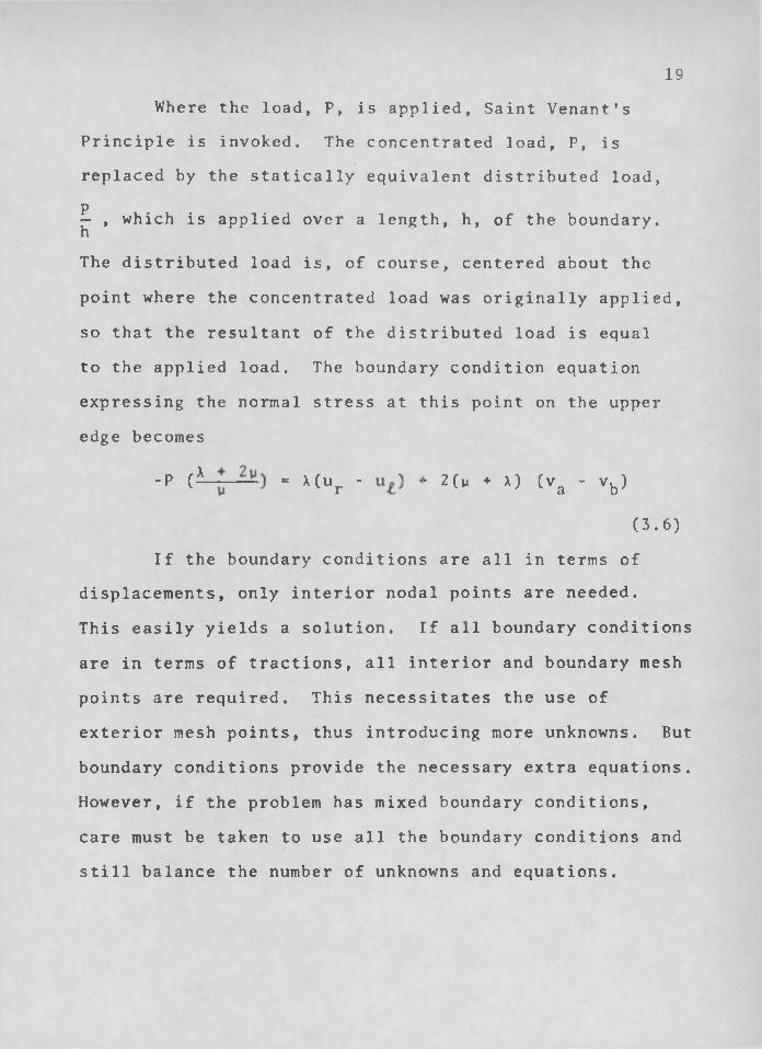
19Where the load, P, is applied, Saint Venant's

Principle is invoked. The concentrated load, P , is

replaced by the statically equivalent distributed load,p— , which is applied over a length, h, of the boundary, hThe distributed load is, of course, centered about the

point where the concentrated load was originally applied,

so that the resultant of the distributed load is equal

to the applied load. The boundary condition equation

expressing the normal stress at this point on the upper

edge becomes

-p (x I — ) = x(ur - u t 2(11 + X) (va - vb)

(3.6)

If the boundary conditions are all in terms of displacements, only interior nodal points are needed.

This easily yields a solution. If all boundary conditions

are in terms of tractions, all interior and boundary mesh

points are required. This necessitates the use of

exterior mesh points, thus introducing more unknowns. But

boundary conditions provide the necessary extra equations.

However, if the problem has mixed boundary conditions,

care must be taken to use all the boundary conditions and

still balance the number of unknowns and equations.

Transition Points

In the plate shown in Figure 1, and in general in

any mixed boundary value problem of this type, Navier's

Equations must be applied to every interior nodal point

and to any boundary point where displacements are not

specified. When Navier's Equations are appled to these

boundary points, exterior mesh points will be introduced

as unknowns. But the tractions specified at these points

will provide extra equations to balance these exterior

unknowns. The problem occurs in applying Navier's

Equations to a transition point. A transition point is

any boundary point where tractions are specified and a

neighboring boundary point has its displacement specified.

In order to apply Navier's Equations to such a point, the

displacements of the nodes exterior to the neighboring

nodes are introduced. But since the neighboring nodes

have their displacements specified, there are no

additional equations to balance this additional exterior

unknown, This difficulty is remedied by expressing the

mixed derivatives in Navier's Equations in terms of

inward differences before they are applied to a transition

boundary point.

21For the problem shown in Figure 1, due to symmetry

conditions, only one quarter of the plate must be solved.

For the purpose of discussion, consider the upper right

quarter of the plate shown in Figure 3 with the coarsest

possible mesh superimposed upon it.

The transition point for this problem is the point

marked with an X in Figure 3. For this point, the finite

difference equations take the form

0 = (1 + C) (ur - 2Ui ♦ U£) + £ (vrbb - Vfbb

* 4vrb + 4vlb + 3vr - 3v£) + ua " 2ui " u b

+ h 2Fl

and 0 “ (1 + C) (va - 2v. + vb) + ^ (urbb - "fbb

‘4urb + 4uZb + 3ur ' 3uZ) + vr - 2v. ♦ vI

* h2F2(3.7)

The mixed derivatives have been expressed in terms of?inward differences which also have an h error.

22

r

\

L/2

J

Figure 3

Coarse Mesh Superimposed on One

Quarter of the Clamped Plate

Edges of the quarter plate Superimposed mesh lines

23Summary

Summarizing, the finite-difference equations which

are used to solve the flat plate problem are given below.

Navier’s Equations, Equations (3.2), in terms of

central differences, neglecting body forces are

2(2 + C)Ui = (1 + C) (ur + | (var - vbr

- va£ + v b + ua + ub

and 2(2 ♦ C)v. - (1 ♦ C) (va ♦ vb) ♦ ̂ (uar - ua£ - ubr

* ub P + V r (3.8)

which are applied at all interior nodes and boundary nodes

where tractions are specified except transition points.

Navier’s Equations with mixed derivatives in terms

of inward differences, Equations (3.7), neglecting body

forces, are

2(2 ♦ C)Ui - (1 ♦ C) (ur (vbbr ' vbb£

”4vbr + 4vbZ + 3vr ' 3vz) * ua + ub

and 2(2 ♦ O v j « (1 + C) (va + vb) + ̂ (ubbr - ubb(

-4ubr * 4ubZ + 3ur • 3"f) * v t * v l

(3.9)

which are applied at transition node points.

24Boundary Condition Equations are:

Equation (3.4)

ui * ubb + v b l ' vbr C-10)

which is applied at all exterior points where tractions are specified.

Equation (3.6)

v. - vbb - P--( > — ---(3.11)1 D 2 (ii + X)

which is applied at the node exterior to the point where

the load, P, acts,

and Equation (3.5)

v ‘ - ^

which is applied at all exterior nodes where tractions are

specified, except where Equation (3.11) is applied.

The equations listed in the summary refer to the

displacements of the it^ nodal point in terms of the dis­

placements at neighboring nodal points. All these equations?have an error of the order of h .

25Stress - Strain Equations

The equations in the summary are the general working

equations, and they yield displacements as results. To

solve for the stresses at all nodal points in the plate,

the stress-strain equations for plane stress must be

expressed as finite-difference equations. The stresses

at the it^ nodal point are:

of inward differences since the displacements of the node

exterior to its adjacent point cannot be given in finite-

dif ference form. The equations for the stresses at the

transition point are:

-r _ 4 v ( y + X)T11 2F(r + 210T _ 4v (u + x)22 T R T x " ” 2 p 1

(3.13)

As before, the transition point requires the use

2yX-4u£ + 3up

2h(X + 2u)

26

and T12 = ^ (ubb ' 4ub * 3ui + 4v£ + 3vi)

(3.14)

With displacements known, Equations (3.13) and

(3.14) easily yield stresses.

Graded Mesh

The finite-difference equations listed above are

derived using a square mesh, so the mesh size can be

expressed in terms of one parameter, h , which is the mesh

spacing. The solution obtained using those equations2contains an error of the order of h .

One method of obtaining a better solution is to

use a finer grid, that is, to reduce the value of h. But

this causes an increase in the number of equations. This,

in turn, increases computer time and expense.

Frequently in a problem of this type, a coarse

mesh is satisfactory over a large portion of the plate,

but a finer mesh is necessary over a critical section.

In the proposed problem, the critical section occurs in

the vicinity of the applied load.

An obvious solution is to superimpose a fine mesh

over the critical region and a coarse mesh over the remain­

der of the plate. Thus, the error in the critical region

is reduced while keeping the number of equations to a

minimum. However, using a graded mesh increases the

complexity of the problem.

27Consider the coarse mesh shown in Figure 3, but

with a finer mesh in the region of the applied load as

shown in Figure 4.

are needed in order to evaluate the displacements at many

of the nodes of the finer mesh. However, these points are

not nodal points, and therefore their displacements at

these points are found by averaging the values of the

displacements at nodes nearby.

the interior of the plate and are in the center of a

mesh square are evaluated by averaging the displacements

at the nodes on the corners of the square. For these

displacements, the equations are

mesh lines, are evaluated by averaging the displacements

at the two nearest nodes. If the point lies on a vertical

mesh line, the equations for its displacements arc

The displacements at the points marked with an X

The displacements of the points, X, which are in

and v. - .25 ( v ^ + ♦ v ^ ) (3.15)

The displacements of the points, X, which are on

and v i (3.16)

28

99 ™ " 9 ” 9 " ^ x I

— ( ) 1 (|)— ^ — — E3—

4 “ - 9 x

Q - -i- -^- - x - -E|3-

| X )( X 9 x^ ------ -E3- — 9 A -

- 9

T\

\

\

■ ^ 9

L/2

i - - e - 4 4— -4i--------- L/2 -------------

Figure 4

Graded Mesh Superimposed on One

Quarter of the Clamped Plate

Edges of the quarter plate Superimposed mesh lines

29

If the point lies on a horizontal mesh line, the equations for its displacements are

u. = .5 (ur + u^)

and v . = .5 (vr + v^) (3.17)

For the point, X, exterior to the plate but not on

a mesh line, the boundary-condition equations are used.

The displacements at the nodes marked with a

circle,O, are evaluated using the general working equations

as if only the fine mesh were used for the entire plate.

The displacements at the nodes marked with a square, D ,

are evaluated using the general working equations as if

only the coarse mesh were used.

This averaging process is actually an application

of Bessel’s Formula for Interpolating to Halves

(Scarborough 1958, p. 77) using only first differences.

If the change were something other than halving the coarse

mesh, a more general interpolation formula must be used.

CHAPTER IV

METHODS OF SOLUTION

Numerical Solution

There are many schemes which may be used to solve a

system of linear algebraic equations such as the system

generated by the finite-difference equations applied to

this problem. Because of the large number of equations

and the ready availability of the IBM 7072 digital computer,

the Gauss - Seidel Method of Iteration was chosen as the

method of solution. The equations in Chapter III were

formulated for an iterative solution; that is, each

equation expresses the displacement at a node in terms of

displacements at neighboring nodes.

It is well known that the method of iteration

often uses a relatively large amount of computer time„

In an effort to minimize the computer time, a scheme to

accelerate the convergence of the set of equations is used.

This scheme is presented by Faddeeva (1959). It consists

in extracting the dominant eigenvalue of the iteration

matrix, and using this eigenvalue in an equation to extra­

polate to new values of displacements in place of an

iteration.

30

31The two extrapolation equations are

1 - K Cn-1) „ (n-2)

and = v("-2) » li--------II---- (4.1)1 1 1 - K

where n designates the extrapolated values n-1 designates

the last iteration value, and n-2 designates the next to

the last iteration value. K is the dominant eigenvalue.

The proposed problem was solved using the iteration

method with Faddeeva’s acceleration scheme for three

different mesh sizes. First, a solution was obtained

using a coarse mesh with h®i- as shown in Figure 3. The

second and third solutions were obtained using a middle-

sized mesh with h=— and a fine mesh with h=^— „ The12 24computer program used for the fine mesh is given in the

Appendix.

As a comparison, the problem was also solved for

the same three mesh sizes using the Gauss - Seidel Method

of Iteration without Faddeeva‘s acceleration scheme.

Also, in order to determine the feasibility of

varying the mesh size, solutions were obtained for the

proposed problem using a coarse graded mesh of size h=—6

32Lwith a mesh of size h^yy the vicinity of the load as

Tshown in Figure 4, and a fine graded mesh of size h=yy

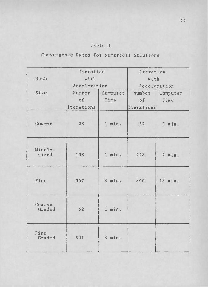
with a mesh of size h=— in the vicinity of the load.24The convergence rates of the different solutions

are listed in Table 1. The IBM 7072 lists total time used

in one minute increments, so for the solutions which took two minutes or less, the number of iterations is a better

measure of the difference in convergence rates. The most

dramatic difference occurs in the comparison of the

convergence rate of the fine mesh solution using Faddeeva*s

acceleration scheme with that of the fine mesh solution

using only iteration.

From the results in Table 1, it can be stated that

the solution of a system of linear algebraic equations will

converge approximately twice as fast using Faddeeva1s

acceleration scheme as the same system without the

acceleration scheme. This estimate is based on the

relative convergence rates of only three systems of

equations. More investigation is necessary before any

authoritative statement regarding Faddeeva's acceleration

scheme can be made. However, the results in Table 1

indicate that such an investigation could be very fruitful.

33

Table 1

Convergence Rates for Numerical Solutions

Mesh

Size

I teration wi th

Acceleration

Iterationwith

AccelerationNumber

ofIterations

Computer T ime

Numberof

Iterations

Computer T ime

Coarse 28 1 min. 67 1 min.

Middle-sized 108 1 min. 228 2 min.

Fine 367 8 min. 866 18 min.

CoarseGraded 62 1 min.

FineGraded 501 8 min.

34As stated previously, a numerical solution of

Navier*s Equations yields displacements. Using the

finite-difference form of the stress-strain equations,

vertical and horizontal normal stresses with the associated

shear stresses were obtained. Through the Mohr's Circle

relationships, maximum shear stress was obtained at all

node points on the plate. A graphical comparison of the

stresses with the photelastic solution is presented in

Chapter V of the thesis.

Photoelastic Solution

Photoelasticity is a standard method employed in

plane stress analysis (Jessop and Harris 1950, Lee 1950).

In this thesis, the photoelastic method was used to

determine the isochromatic lines, that is the lines of

constant maximum shear stress in a model which is shaped,

supported, and.loaded in the same manner as the plate in

the proposed problem.

Before the model can be tested, the model constant

must be determined. This constant is a function of the

thickness and the optical properties of the model material.

The material used was CR-39 with a thickness of .25 inches.

Using the standard beam method of calibration (Lee 1950,

pp. 166-167), the model constant was found to be 175 psi.

per fringe.

35Figure 5 is a photograph of one quarter of the

3-inch by 3-inch photoelastic model with a vertical applied

load of 405 pounds. The upper right corner is the point

of application of the load, the lower right corner is the

middle of the plate, and the left edge is clamped. The

wide, dark curve in the upper right corner marks the edge

of a local lens formed by relatively large displacements

normal to the plate in the vicinity of the applied load.

The oyster shell figure is the left of this lens is caused

by a small crack in the material at that point. As the

applied load was increased from 0 to 405 pounds, it was

observed that the lens and the crack affected the fringe

pattern only in their immediate vicinity. The dark spot on the left side of the lower edge is a point of zero

maximum shear stress. The closest dark line to this zero

point is the locus of points with maximum shear stress

equal to 17 5 psi. Each succeeding dark line is the locus

of points where the maximum shear stress is increased by

175 psi. over that of the previous line. So from the

photograph, the distribution of maximum shear stress over

the plate can be determined.

Although the photoelastic solution is used in this

thesis as a check on the accuracy of the numerical solution,

the maximum shear stresses obtained by the photoelastic

method contain errors due to imperfections in the optical

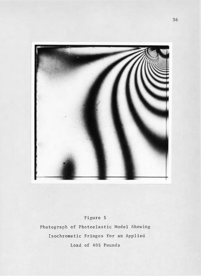
Figure 5

Photograph of Photoelastic Model Showing

Isochromatic Fringes for an Applied

Load of 405 Pounds

37system used, methods of machining and loading the model,

and interpolation in reading the photograph. Considering

all these causes, the total error in the photoelastic

solution is estimated to be one-half of a fringe or

approximately 88 psi.

CHAPTER V

RESULTS AND CONCLUSIONS

To compare the results of the numerical and photo­

elastic methods of solution, the maximum shear stress for

both methods is shown in graphical form for an applied

load of 405 pounds in Figure 6 and Figure 7.

Figure 6 is a graph of maximum shear stress versus

position on the plate along a vertical line from the load

point to the middle of the plate. Figure 7 is the same

type of graph along a horizontal line from the middle of

the plate to the clamped edge. Together these graphs

display the variation of shear stress from a maximum to a

minimum value on the plate.

Accuracy of Numerical Solutions

The finite-difference representations of the govern­

ing differential equations contain an error proportional

to the square of the mesh spacing and the gradient of the

displacements in the plate. For the numerical solutions

with constant mesh size, the least error would be expected

in those regions of the plate where the displacements

varied the least. However, considering the round-off

errors and the convergence test in the computational

38

Figure 6Maximum Shear Stress as a Function of Position

from the Load Point to the Middle of the Plate

Curve 1 the coarse mesh solution Curve 2 -- the coarse graded mesh solution Curve 3 the middle-sized mesh solution Curve 4 the fine graded mesh solution Curve 5 -- the fine mesh solution Curve 6 -- the photoelastic solution

The photoelastic solution is shown in its entirety as well as the photograph could be read. The curves of the numerical solutions are discontinued for clarity. The portions of the curves which are omitted all lie within 60 psi. of the photoelastic solution. On the abscissa, the zero point is the point of application of the load and L/2 is the middle of the plate =

Maximum

Shear

Stress

in psi.

39

2400

2000

1600

1200

800

400

0 L L 3L

Position

Figure 6

Maximum Shear Stress as a Function of Position

from the Load Point to the Middle of the Plate

wit—

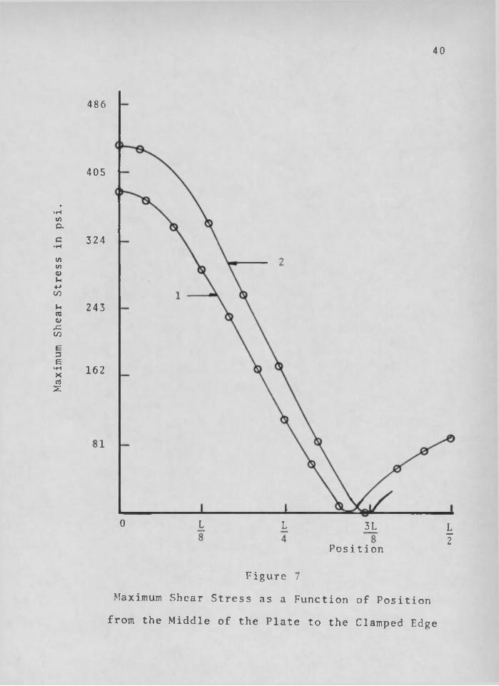
Figure 7

Maximum Shear Stress as a Function of Position

from the Middle of the Plate to the Clamped Edge

Curve 1 -- the fine mesh solution Curve 2 -- the photoelastic solution

The photoelastic solution is shown in its entirety as well as the photograph could be read. For clarity, the other four numerical solutions are omitted. All portions of the omitted curves lie within 60 psi. of the photoelastic solution. On the abscissa, the zero point is the middle of the plate and L/2 is the clamped edge.

Maximum

Shear

Stress

in psi.

40

486

405

324

243

162

1

0 L L 3L

Pos i t ion

Figure 7

Maximum Shear Stress as a Function of Position

from the Middle of the Plate to the Clamped Edge

fo|r-

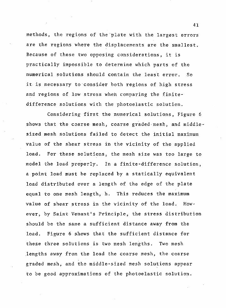
41

methods, the regions of the "plate with the largest errors

are the regions where the displacements are the smallest.

Because of these two opposing considerations, it is

practically impossible to determine which parts of the

numerical solutions should contain the least error. So

it is necessary to consider both regions of high stress

and regions of low stress when comparing the finite-

difference solutions with the photoelastic solution.

Considering first the numerical solutions. Figure 6

shows that the coarse mesh, coarse graded mesh, and middle-

sized mesh solutions failed to detect the initial maximum

value of the shear stress in the vicinity of the applied

load. For these solutions, the mesh size was too large to

model the load properly. In a finite-difference solution,

a point load must be replaced by a statically equivalent

load distributed over a length of the edge of the plate

equal to one mesh length, h. This reduces the maximum

value of shear stress in the vicinity of the load. How­

ever, by Saint Venant1s Principle, the stress distribution

should be the same a sufficient distance away from the

load. Figure 6 shows that the sufficient distance for

these three solutions is two mesh lengths. Two mesh

lengths away from the load the coarse mesh, the coarse

graded mesh, and the middle-sized mesh solutions appear

to be good approximations of the photoelastic solution.

42The fine graded mesh and the fine mesh solutions

also contain a large error in the vicinity of the applied

load. However, due to the smaller mesh size, they more

closely approximate the steep gradient in the shear stress

in the vicinity of the load. Again, these solutions are

good approximations to the photoelastic solution at any

point in the plate at least two mesh lengths away from

the load point. It should be mentioned here that, due

to the local lens, the photoelastic results are of question­

able accuracy within two fine mesh lengths of the applied

load.

Photoelastic Solution as a Measure of the Accuracy of

the Numerical Solutions

From the curves in Figure 6 and Figure 7, the

numerical solutions are all within 160 psi. of the

photoelastic solution for all points at least two mesh

lengths away from the applied load. The coarse mesh,

coarse graded mesh, and middle-sized mesh solutions must

be regarded as poor approximations to the photoelastic

solution due to their inability to detect the large

stress gradient in the vicinity of the load.

The fine graded mesh and the fine mesh solutions

have a small enough grid spacing to detect the initial

steep gradient in the maximum shear stress. These two

solutions are within 120 psi. of the photoelastic solution

43for an applied load of 405 pounds. The largest maximum

shear stress in the plate is approximately 2400 psi. So

the error in these two numerical solutions as compared to

the photoelastic solution is 5 per cent of the largest

maximum shear stress. Of course, in the regions of low

maximum shear stress, the percentage error is large, but

the region of high shear stress is of greatest interest,

and here the percentage error is low. From economic

considerations, it is difficult to choose between the

fine graded mesh and the fine mesh solutions, since

they both ran eight minutes on the IBM 7072 computer.

The fine graded mesh solution was designed to

yield results comparable to the fine mesh solution in

the vicinity of the load while saving computer time by

using fewer nodal points and therefore having to solve

a smaller set of equations. However, the computer program

used for the graded mesh solution was written in a form

which minimized programming difficulties but not computa­

tion time. Had computation time been the prime con­

sideration, the fine graded mesh would have yielded a

solution in approximately 30 per cent less time than the

fine mesh. This estimate is based upon the relative

convergence rates of the middle-sized mesh and coarse

graded mesh solutions as listed in Table 1, and applies

only to the specific problem proposed in this thesis.

44Therefore> considering economy and accuracy, the

fine graded mesh solution provides the best approximation

to the photoelastic solution for the problem proposed in

this thesis.

Conclusions

The study undertaken in this thesis leads to three

conclusions.

First, the finite-difference solution of Navier1s

Equations yields a good approximate solution to a mixed

boundary-value problem in plane elasticity. This, of

course, presupposes that a sufficiently small mesh is

used.

Second, Faddeeva1s acceleration scheme can reduce

convergence time by one half for an iterative solution of a system of linear algebraic equations. Perhaps with a

different system of equations, even better results could

be obtained.

Third, a variable mesh procedure should be employed

in order to model an applied load more accurately or to

detect regions where the displacement gradient is large.

This will increase the accuracy of the finite-difference

solution in the regions of greatest interest while keep­

ing the computation time to a minimum.

45Proposal for Future Investigation

The results of this thesis indicate the desir­

ability of further investigation into Faddeeva1s

acceleration scheme. Faddeeva1s scheme was applied to

three sets of equations in this thesis and increased

their convergence rates by 50 per cent. This is a sub­

stantial saving in computer time. However, before any

broad statement concerning Faddeeva * s scheme can be made,

it must be tested on many different sets of equations.

One important aspect of Faddeeva * s acceleration

scheme is that the slower the convergence of the iterative

solution, the more effective the acceleration scheme. This

is due to the fact that the dominant eigenvalue of the

iteration matrix, which is a measure of the rate of

convergence, is used to accelerate the convergence. So

any future investigation should include a few sets of

equations with a relatively fast rate of convergence

and a larger number with a relatively slow rate of con­

vergence . In this way, it would be possible to measure,

over a large range, the percentage of computer time saved

using Faddeeva1s acceleration scheme.

Professor Richmond C. Neff of the University of

Arizona has presented in his lectures an acceleration

scheme which is, in effect, a higher order form of

Faddeeva’s scheme. This higher order acceleration scheme

46consists in extracting the first two or three dominant

eigenvalues and using these to accelerate the rate of

convergence. The higher order method could be of

significant value whenever the first two or three

dominant eigenvalues have approximately the same

magnitude. This scheme was not used in this thesis, but

due to the success of Faddeeva's scheme, any future

investigation should give the higher order scheme serious

consideration.

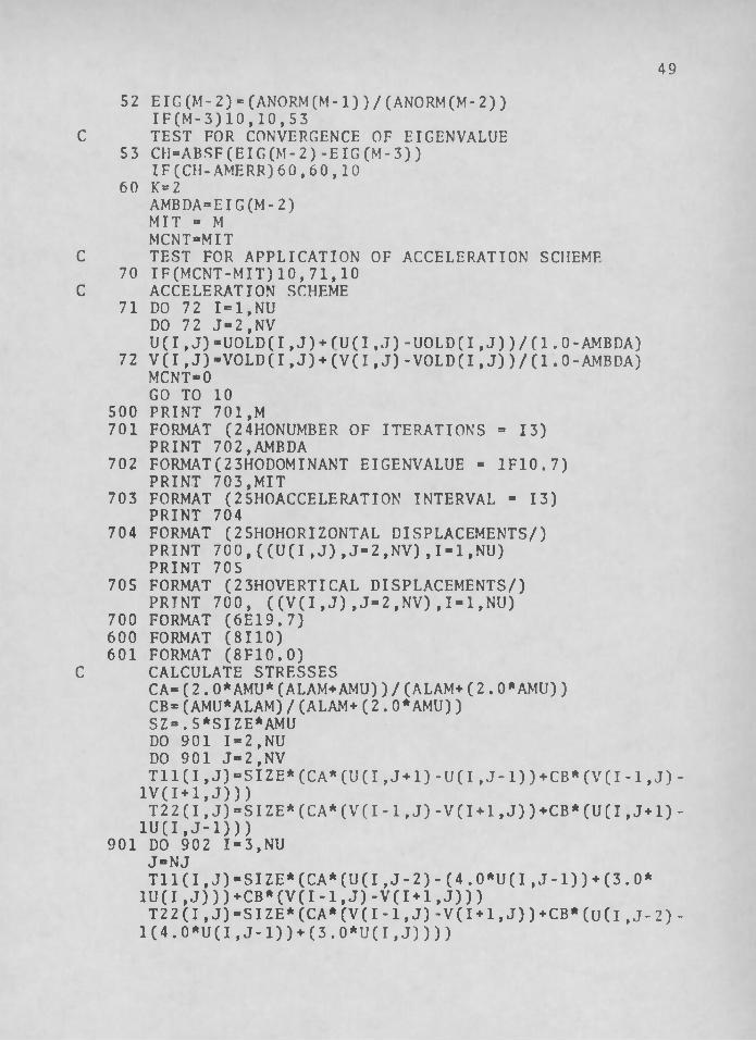
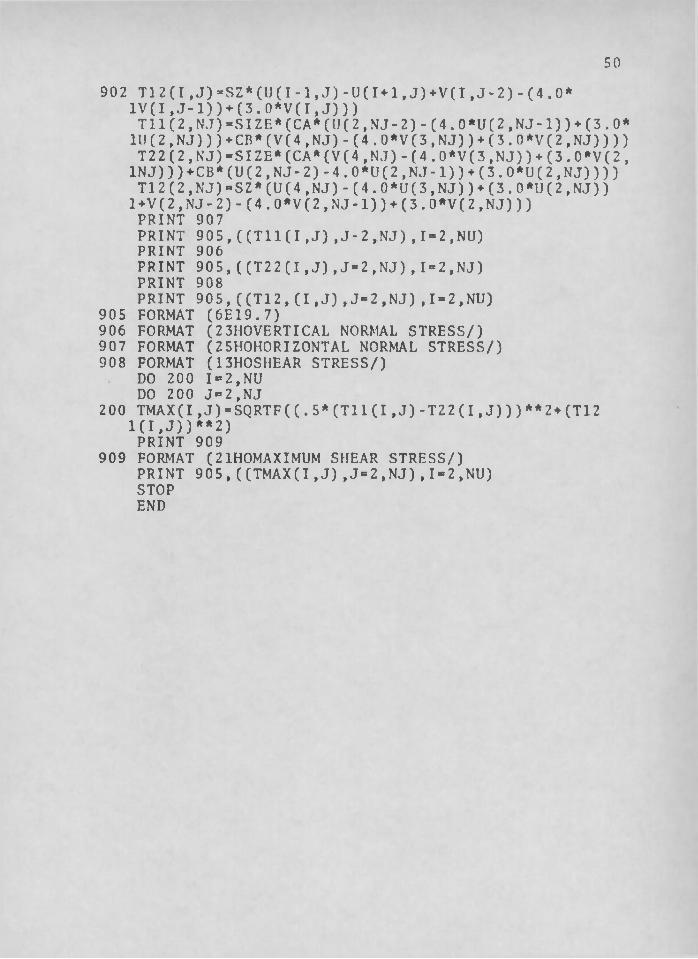
APPENDIX

The following is the computer program used to

solve the flat plate problem using the fine mesh. The

program is written in Fortran II language and was run

on the IBM 7072 computer at the University of Arizona.

C GAUSS-SEIDEL ITERATION WITH AN ACCELERATION SCHEMEC BY FADDEEVA

DIMENSION UOLD(15,15),VOLD(15,15),U(15,15),V(15,15), 1SUMX(900),ANORM(899),EIG(898),TSUMX(900),ANORT(899), 2T11(15,1S),T22(15,15),T12(15,15),TMAX(15,15)READ 600,NI,NJ,MERRREAD 601,AMERR,CONST,ALAM,AMU,PREAD 601,SIZEK® 1M= 0MCNT®0 NU=NI-1 NV-NJ-1 DO 1 1=1,NI DO 1 J=1,NJ U(I,J)-0.0

1 V(I,J)=0.010 M=M+1

MCNT=MCNT+1C TEST FOR NUMBER OF ITERATIONS

IF(M-MERR)11,11,50011 DO 12 1=1,NU

DO 12 J* 2,NV UOLD(I,J)=U(I,J)

12 VOID(I ,J)=V(I,J)DO 90 J=2,NVDO 89 1=1,NU DO 13 L=1,NU

C SYMMETRY CONDITIONSU(L,1)=-U(L,3)

13 V(L,1)=V(L,3)DO 14 L=2,NVV(15,L)*-V(13,L)

14 U (15,L)=U(13,L)I F ( I - 1 ) 1 5 , 2 5 , 1 5

47

4815 IF(J-2)16,26,1616 IF(I-14)17,27,1717 IF(I-2)24,18,2418 IF(J-13)24,28,24

C WORKING EQUATIONS2 4 U(I,J)=((1.O+CONST)*(U(I,J+1)+U(I,J-1))+(CONST/4.0)*

1(VI-1,J+1)-V(I+1,J*1)-V(I-1,J-1)+V(I*1,J-1)) 2*U(I-1,J)+U(1*1,J))/(2.0*(2.O+CONST))

33 V(I,J)«=((1. O+CONST) *(V(I-1,J)+V(I + 1,J)) + (CONST/4 .0) * 1(U(I-1,J+1)-U(I-1,J-1)-U(I+1,J+1)+U(I+1,J-1)) 2+V(I,J+l)+V(I,J-l))/(2.0*(2.O+CONST))GO TO 89

25 U(I,J)-U(I+2,J)+V(I+1,J-I)-V(I+1,J+1)IF(J-2)31,32,31

31 V(I,J)«(-ALAM*(U(I+1,J+1)-U(I+1,J-1)))/(2.0*(AMU+ 1ALAM))+V(I+2,J)GO TO 89

3 2 V(I,J)- (-P*((ALAM+2.0*AMU)/AMU)-ALAM*(U(1+1,J+1)-lU(I+l,J-l)))/(2.0*(AMU+ALAM))+V(I+2,J)GO TO 89

26 IF(I-14)33,89,3327 U(I,J)=((1.O+CONST)*(U(I,J+1)+U(I,J-1))+(CONST/4.0)*

1(V(I-1,J+1)-V(I+1,J+1)-V(I-1,J-1)+V(I+1,J-1)) 2+U(I-l,J)+U(I+l,J))/(2.0*(2.O+CONST)GO TO 89

2 8 U(I,J)-((l.O+CONST)*(U(I,J+1)+U(I,J-1))+(CONST/4.0)* 1(V(I+2,J+1)-V(I+2,J-1)-4,0*V(I+1,J+1)+4.0*V(I+1,J-1) 2+3.0*V(I,J+l)-3.0*V(I,J-l))+U(I-l,J)+U(I+l,J))/(2.0* 3(2.O+CONST))V(I,J)=((1.O+CONST)*(V(I-1,J)+V(I+1,K))+(CONST/4.0)* 1(U(1+2,J+L)-U(I+2,J-1)-4.0*U(I+1,J+1)+4.0*U(I+1,J-1) 2+3.0*U(I,J+l)-3.0*U(I,J-l))+V(I,J+l)+V(I,J-l))/(2.0* 3(2.O+CONST))GO TO 89

89 CONTINUE90 CONTINUE39 SUMX(M)=0.0

TSUMX(M)-0.0 DO 40 1=1,NU DO 40 J-2,NVTSUMS(M)=TSUMX(M)+ABSF(U(I,J))+ABSF(V(I,J))

40 SUMX(M)=SUMX(M)+U(I,J)+V(I,J)IF(M-1)10,10,41

41 ANORM(M-l)=SUMX(M)-SUMX(M-l)ANORT(M-l)=ABSF(TSUMX(M)-TSUMX(M-l))IF(M-2)10,10,50

C TEST FOR CONVERGENCE OF SYSTEM50 TEST-ABSF(ANORT(M)-ANORT(M-1))

IF(TEST-.001*ANORT(M))500,500,5151 IF(K-1) 52 ,52, 70

4952 EIG(M-2)=(ANORM(M-1))/(ANORM(M-2))

IF(M-3)10,10,53C TEST FOR CONVERGENCE OF EIGENVALUE

53 CH«ABSF(EIG(M-2)-EIG(M-3))IF(CH-AMERR)60,60,10

60 K=2AMBDA=EIG(M-2)MIT - M MCNT-MIT

C TEST FOR APPLICATION OF ACCELERATION SCHEME70 IF(MCNT-MIT)10,71,10

C ACCELERATION SCHEME71 DO 72 1=1,NU

DO 72 J=2,NVU(I,J)=UOLD(I,J)+rU(I,J)-UOLD(I,J))/(1.0-AMBDA)

72 V(I,J)-VOLD(I,J)*(V(I,J)-VOLD(I,J))/(1.0-AMBDA) MCNT-0GO TO 10

500 PRINT 701,M701 FORMAT (24HONUMBER OF ITERATIONS = 13)

PRINT 702,AMBDA702 FORMAT(23HODOMINANT EIGENVALUE = 1F10.7)

PRINT 703,MIT703 FORMAT (25HOACCELERATION INTERVAL = 13)

PRINT 704704 FORMAT (2 5HOHORIZONTAL DISPLACEMENTS/)

PRINT 700,((U(I,J),J=2,NV),I=1,NU)PRINT 705

705 FORMAT (23HOVERTICAL DISPLACEMENTS/)PRINT 700, ((V(I,J),J=2,NV),I=1,NU)

700 FORMAT (6E19.7)600 FORMAT (8110)601 FORMAT (8F10.0)

C CALCULATE STRESSESCA=(2.0*AMU*(ALAM+AMU))/(ALAM+(2.0*AMU))CB=(AMU*ALAM)/ (ALAM+(2.0*AMU))SZ=.5*SIZE*AMU DO 901 1=2,NU DO 901 J-2.NVT11(I,J)=SIZE*(CA*(U(I,J + 1)-U(I,J-1)) + CB*(V(I-1,J) - 1V(I+1,J)))T2 2(I,J)=SIZE*(CA*(V(I-1,J)-V(I+1,J))+CB*(U(I,J+1)- 1U(I,J-1)))

901 DO 902 1=3,NU J-NJTll(I,J)»SIZE*(CA*(U(I,J-2)-(4.0*U(I,J-l))+(3.0* 1U(I,J)))+CB*(V(I-1,J)-V(I+1,J))) T22(I,J)=SIZE*(CA*(V(I-l,J)-V(I*l,J))*CB*(u(l,J-2)- 1(4.0*U(I,J-1))+(3.0*U(I,J))))

50902 T12(I,J)”SZ*(U(I-l,J)-U(I+l,J)+V(I,J-2)-(4.0*

1V(I,J-1))*(3.0*V(I,J))) Tll(2,N.T)-SIZE*(CA*(V(2,NJ-2) -(4.0*U(2,NJ-l)) + (3.0* ll)(2,NJ)))*CR*(V(4,NJ)-(4.0*V(3,NJ)) + (3.0*V(2,NJ)))) T22(2,NJ)-SIZE*(CA*(V(4,NJ)-(4.0*V(3,NJ))+(3.0*V(2, lNJ)))+CB*(U(2,NJ-2)-4.0*U(2 ,N,I -1)) + (3.0*U(2,NJ)))) T12(2,NJ)-SZ*(U(4,NJ)-(4.0*U(3,NJ))*(3.0*U(2,NJ)) l*V(2,NJ-2)-(4.0*V(2,NJ-1))+(3.0*V(2,NJ)))PRINT 907PRINT 905,((Til(I,J),J-2,NJ),I=2,NU)PRINT 906PRINT 905,((T22(I,J),J=2,NJ),1=2,NJ)PRINT 908PRINT 905, ((T12, (I ,J) ,J*2,NJ) ,1 = 2,Nil)

905 FORMAT (6E19.7)906 FORMAT (2 3HOVERTICAL NORMAL STRESS/)907 FORMAT (25HOHORIZONTAL NORMAL STRESS/)908 FORMAT (13HOSHEAR STRESS/)

DO 200 1=2,NUDO 200 J=2,NJ

200 TMAX(I,J)=SQRTF((.S*(T11(I,J)-T22(I,J)))**2*(T12 1(I,J))**2)PRINT 909

909 FORMAT (21HOMAXIMUM SHEAR STRESS/)PRINT 905,((TMAX(I,J),J=2,NJ),1=2,NU)STOPEND

REFERENCES

Allen, D . N. de G ., Relaxation Methods in Engineering and Science, McGraw-Hill Book Company, Inc. ,!TewTorIqrTPS4.

Boresi, Arthur P., Elasticity in Engineering Mechanics,Prentice-HalY^ Inc., Englewood Cliffs, New Jersey, 1965.

Faddeeva, V. N., Computational Methods of Linear Algebra, Dover Publications, Inc., New YorF, 19^9.

Griffin, D. S. and R. S. Varga, "Numerical Solution ofPlane Elasticity Problems," Journal of the Society for Industrial and Applied Mathematics, Vol. ITT No". 4, December, 1963, pp. 1046-62.

Jessop, H. T. and F. C. Harris, Photoelasticity:- Principle and Methods, Dover Publications, Inc., New York, 19 50.

Lee, George Hamor, An Introduction to Experimental Stress Analysis, John Wiley 6 Sons,Inc.,New York, 1950.

Salvadori, Mario G. and Melvin L . Baron, NumericalMethods in Engineering, 2nd Edition, Prentice- Hall, Inc., Englewood Cliffs, New Jersey, 1961.

Scarborough, James B ., Numerical Mathematical Analysis, 4th Edition, The Johns Hopkins Press, Baltimore, 1958.

Sokolnikoff, I. S . , Mathematical Theory of Elasticity,2nd Edition, McGraw-Hi11 Book Company, Inc.,New York, 1956.

51