Curved Folding

Martin KilianTU Vienna

Evolute

Simon FloryTU Vienna

Evolute

Zhonggui ChenTU Vienna

Zhejiang University

Niloy J. MitraIIT Delhi

Alla ShefferUBC

Helmut PottmannTU Vienna

Figure 1: Top left: Reconstruction of a car model based on a felt design by Gregory Epps. Close-ups of the hood and the rear wheelhouse areshown on the left. The fold lines are highlighted on the car’s development. Top right and bottom: Architectural design. All shown surfacescan be isometrically unfolded into the plane without cutting along edges and can thus be texture mapped without any seams or distortions.

AbstractFascinating and elegant shapes may be folded from a single planarsheet of material without stretching, tearing or cutting, if one incor-porates curved folds into the design. We present an optimization-based computational framework for design and digital reconstruc-tion of surfaces which can be produced by curved folding. Ourwork not only contributes to applications in architecture and indus-trial design, but it also provides a new way to study the complexand largely unexplored phenomena arising in curved folding.

CR Categories: I.3.5 [Computer Graphics]: Computational Ge-ometry and Object Modeling—Geometric algorithms, languages,and systems; I.3.5 [Computer Graphics]: Computational Geometryand Object Modeling—Curve, surface, solid, and object represen-tations

Keywords: computational differential geometry, computationalorigami, architectural geometry, industrial design, developable sur-face, folding, curved fold, isometry, digital reconstruction.

1 Introduction

Developable surfaces appear naturally when spatial objects areformed from planar sheets of material without stretching or tear-ing. Paper models such as origami art are prominent exam-ples. The striking elegance of models folded from paper, suchas those by David Huffman [Wertheim 2004], arises particularlyfrom creases known as curved folds. Such folds can be gener-ated from a single planar sheet. Early investigations of curvedfolds are due to Huffman [1976]. More recently, computationalgeometers became interested in folding problems and computa-tional origami [Demaine and O’Rourke 2007]. Their work concen-trates on piecewise linear structures; according to [Demaine andO’Rourke 2007], ‘little is known’ in the curved case. While indus-trial designers have started to explore the technique of curved fold-ing (www.curvedfolding.com), current geometric modeling sys-tems still lack any support for such a design process (in fact, mostCAD systems are lacking a proper treatment of developable sur-faces). As a result, Frank O. Gehry, who favors developable shapesfor many of his architectural designs (cf. [Shelden 2002]), has ini-tiated the development of a CAD module for developable surfacesby his technology company. To the best of our knowledge, curvedfolding is not present in that module either.

Motivated by the potential and interest in the use of curved fold-ing for various geometric design purposes, we investigate this topicfrom the perspective of geometric modeling.

Related work. Developable surfaces are well studied in differen-tial geometry [do Carmo 1976]. They are surfaces which can be un-folded into the plane while preserving the length of all curves on the

Figure 2: The car model of Figure 1 and its development (topright). The patch decomposition into torsal ruled surfaces is shownusing the following color scheme: planes are shown in yellow,cylinders in green, cones in red, and tangent surfaces in blue. Sam-ple rulings are shown on some patches of the windshield and theside window. Such a segmentation is essential for NURBS surfacefitting and manufacturing.

surface. Developable surfaces are composed of planar patches andpatches of ruled surfaces with the special property that all pointsof a ruling have the same tangent plane. Such torsal ruled surfacesconsist of pieces of cylinders, cones, and tangent surfaces, i.e., theirrulings are either parallel, pass through a common point, or are tan-gent to a curve (curve of regression), respectively. Whereas a torsalruled surface has only one continuous family of rulings, generalsmooth developable surfaces are usually a much more complicatedcombination of patches. The presence of planar parts is the mainsource of this huge variety of possibilities. The level of difficulty isfurther increased if one admits creases, i.e., curved folds (see Fig-ure 2).

In geometric design, various ways of treating developability havebeen pursued: as a constraint in tensor product B-spline surfacesof degree (n, 1) [Chu and Sequin 2002; Aumann 2004], aimingonly at approximate developability [Perez and Suarez 2007], view-ing the surfaces as sets of their tangent planes [Pottmann and Wall-ner 2001], subdividing strips of planar quads [Liu et al. 2006], orcomputing with triangle meshes and a local convexity constraint[Frey 2004; Wang and Tang 2004; Subag and Elber 2006; Wang2008]. Bo and Wang [2007] model paper strips as rectifying devel-opables of one of their geodesics. Digital reconstruction of torsalruled surfaces employing a plane-geometric approach is the topicof [Peternell 2004].

Mesh parametrization and segmentation using developable surfaceshas been investigated in [Julius et al. 2005] and [Yamauchi et al.2005]. Rose et al. [2007] show how to compute developable sur-faces from boundary curves, and present a strategy for selecting anoptimal solution. Several algorithms have been proposed for theconstruction of papercraft models [Mitani and Suzuki 2004; Mas-sarwi et al. 2006; Shatz et al. 2006] using folds along line seg-ments. In all these papers, triangle meshes are used to representdevelopable surfaces.

Only a few contributions deal with the difficult analysis and compu-tation of creases in developable surfaces. Most of them concentrate

on conical creases [Kergosien et al. 1994; Cerda et al. 1999; Frey2004]. Starting from conical folds, Cerda et al. [2004] investigatedgravity-induced draping of naturally thin flat sheets.

Contributions and overview. We present an optimization-basedcomputational framework for the design and reconstruction of gen-eral developable surfaces with a strong focus on curved folding ap-plications. Our main contributions are as follows:

�We employ quad meshes with planar faces as a discrete differen-tial geometric representation of developable surfaces, and for thisrepresentation introduce new ways of computing curvatures andbending energy. Moreover, we discuss curved folds from the dis-crete perspective (Section 2).

� In Section 3, we introduce the core of our work, a novel opti-mization algorithm which allows us to compute developable sur-faces with curved folds that are isometric to a given planar sheet,while at the same time achieving additional objectives such as ap-proximation of given geometric data, aesthetics, and minimizationof bending energy.

� Section 4 presents various ways in which the basic optimizationalgorithm can be used for design. Even simple applications lead tonew results, such as modeling developable strips of minimal bend-ing energy.

� Another main contribution of our work is digital reconstructionof objects exhibiting developable surfaces with curved folds. Algo-rithms for preprocessing the input data in order to make the algo-rithm of Section 3 applicable to digital reconstruction are discussedin Section 5.

� Combining digital reconstruction, optimization and recently in-troduced algorithms for computing in shape space [Kilian et al.2007] we have a rich toolbox for geometry processing with curvedfolds. This is demonstrated by means of a few application scenariosin Section 6. Finally, we summarize our main results, and addressdirections for future research within the largely unexplored area ofcurved folding.

2 Discrete developable surfaces

Developable surfaces. As our basic representation of devel-opable surfaces we employ quad-dominant meshes with planarfaces, which is also the representation of choice for discrete dif-ferential geometry [Sauer 1970; Bobenko and Suris 2005].

A strip of planar quadrilaterals (Figure 3, left) is a discrete modelof a torsal ruled surface. Such a ‘PQ strip’ can be trivially un-folded into the plane without distortions. The edges where succes-sive quads join together give us the discrete rulings. In general theyform the edge lines of the regression polyline r0, r1, . . . ; in specialcases the discrete rulings are parallel, or pass through a fixed point.A refinement process which maintains planarity of quads generates,in the limit, a torsal ruled surface Σ (Figure 3, right). Its rulings arethe limits of the discrete rulings, which in general are tangent to theregression curve r(t), and in special cases are parallel (cylinder), orpass through a fixed point (cone).

The representation of developable surfaces as PQ strips providesvarious advantages over triangle meshes: (i) developability is guar-anteed by planarity of faces and the development is easily obtained,(ii) subdivision applied to PQ strips provides a simple and compu-tationally efficient multi-scale approach [Liu et al. 2006], (iii) theregression curve – which is singular on the surface and thus needsto be controlled – is present in a discrete form, and (iv) the curvaturebehavior can be easily estimated as shown next.

Curvatures and bending energy. The rulings on a smooth de-velopable surface constitute one family of principal curvature linescorresponding to vanishing principal curvature. The second familyis given by the orthogonal trajectories of the rulings which inte-grate the directions of non-vanishing principal curvatures κ2. Weare interested in a discrete definition of κ2, and the related bendingenergy Ebend =

Rκ2

2dA.

The rulings on a PQ strip are given by the edge lines Ri := piqi

(cf. Figure 4a). As a discrete principal curvature line we take a poly-line C with vertices ci 2 Ri whose edges cici+1 are orthogonal tothe inner bisectors Si ofRi andRi+1. In other words, each edge ofC intersects consecutive rulings at the same angle (this definition isalso motivated by an analogous definition in the context of circularmeshes [Bobenko and Suris 2005]). We want to attach a surfacenormal vector ni to the edge midpoint mi = (ci + ci+1)/2, andtake the normal vector of the plane Pi spanned by edges Ri, Ri+1

for that purpose. The unit vectors fnig form the Gaussian imageof C and thus it is natural to define the principal curvature κ2 at ci

via:

κ2(ci) :=kni − ni− 1k

kci −mi− 1k+ kci −mik= Ni/Li. (1)

This definition has the advantage that the denominator Li can becomputed in the planar development of the strip, while only thenumerator Ni := kni − ni− 1k requires the embedding in space.Note that the curvature κ2 always has a positive sign, in contrast tousual definitions. As we used it in its squared form only, this doesnot matter.

Using the notation of Figure 4 the discrete bending energy Ei =Rκ2

2dA of a region bounded by two discrete principal curvaturelines C, C at distance h := kci − cik and two bisectors Si− 1Si

(depicted by the brown highlight in Figure 4a) is given as

Ei = wikni − ni− 1k2. (2)

The weight wi associated with the ruling Ri is given by

wi = h(ln Li − lnLi)/(Li − Li), (3)

where Li is the denominator of Equation (1). As Li ! Li, in thelimit, we get wi = h/Li. Thus the bending energy of a general PQ

r0

p0

q0

r1

r2

r3r4

c0c1c1c1c1c1c1c1c1c1c1c1c1c1c1c1c1c1

C

P1

r(t)

n1n1n1n1n1n1n1n1n1n1n1n1n1n1n1n1n1 n(t)n(t)n(t)n(t)n(t)n(t)n(t)n(t)n(t)n(t)n(t)n(t)n(t)n(t)n(t)n(t)n(t)

ΣΣΣΣΣΣΣΣΣΣΣΣΣΣΣΣΣ

Figure 3: A PQ strip (left) is a discrete model of a developable sur-face Σ (right). The intersections of edges piqi of adjacent planarquads generate the regression polyline ri. In the limit of a refine-ment process, this regression polyline becomes the regression curver(t). Polylines C, whose edges cici+1 intersect inner bisectors ofconsecutive discrete rulings at right angles, are discrete versionsof principal curvature lines, and serve for the definition of discretecurvatures. The unit normals to planar quads Pi are denoted by ni.

ri

pipipipipipipipipipipipipipipipipi

qiqiqiqiqiqiqiqiqiqiqiqiqiqiqiqiqi

RiRiRiRiRiRiRiRiRiRiRiRiRiRiRiRiRi

Ri+1Ri+1Ri+1Ri+1Ri+1Ri+1Ri+1Ri+1Ri+1Ri+1Ri+1Ri+1Ri+1Ri+1Ri+1Ri+1Ri+1

cicicicicicicicicicicicicicicicici

ci− 1

ci− 1

ci+1ci+1ci+1ci+1ci+1ci+1ci+1ci+1ci+1ci+1ci+1ci+1ci+1ci+1ci+1ci+1ci+1cicicicicicicicicicicicicicicicici

ci+1ci+1ci+1ci+1ci+1ci+1ci+1ci+1ci+1ci+1ci+1ci+1ci+1ci+1ci+1ci+1ci+1

mimimimimimimimimimimimimimimimimi

mi− 1mi− 1mi− 1mi− 1mi− 1mi− 1mi− 1mi− 1mi− 1mi− 1mi− 1mi− 1mi− 1mi− 1mi− 1mi− 1mi− 1SiSiSiSiSiSiSiSiSiSiSiSiSiSiSiSiSi

Si− 1Si− 1Si− 1Si− 1Si− 1Si− 1Si− 1Si− 1Si− 1Si− 1Si− 1Si− 1Si− 1Si− 1Si− 1Si− 1Si− 1

h

CCCCCCCCCCCCCCCCCCCCCCCCCCCCCCCCCC

(a)

(c)

(b)

LiLiLiLiLiLiLiLiLiLiLiLiLiLiLiLiLi

LiLiLiLiLiLiLiLiLiLiLiLiLiLiLiLiLi

Figure 4: (a) The rulings of a PQ strip are given by the edgelines Ri := piqi. The inner bisector of RiRi+1 is denoted bySi. Edges cici+1 of the polyline C intersect Si orthogonally. Ifmi is the mid-point of cici+1, and ni is the normal to the planePi := RiRi+1, then the principal curvature at ci is naturally de-fined by Equation (1). (b) To avoid infinite curvatures at cone ver-tices, computation takes place on a slightly shrunken strip. (c) Thetotal bending energy of a region (brown) bounded by Si− 1Si andtwo principal curvature lines CC is given by Equations (2), (3).

strip can be simply approximated by a sum of energies Ei of thetype (2). Note that we cannot directly apply known formulae fordiscrete bending energies [Desbrun et al. 2005] since those assumethat all edge lengths tend to zero if one passes to the limit. This isnot the case for the rulings in our approach.

Curved folds. In the smooth setting, the following fact aboutcurved folds is well known (see e.g. [Huffman 1976]): At eachpoint of a fold curve c, the osculating plane of c is a bisectingplane of the tangent planes on either side of the fold. This fol-lows immediately from the identical geodesic curvatures of the foldcurve c with respect to the two adjacent developable surfaces S1

and S2. Hence, given the surface on one side of a fold curve, wecan compute (part of) the other as the envelope of planes, obtainedby reflecting the tangent planes about the osculating planes of c.This is discussed in some detail in [Pottmann and Wallner 2001],but one finds only that part of S2 whose rulings meet c. Thus, theapproach is not sufficient for most of our tasks where, in addition,multiple folds may appear, and the locations of such fold curvesonly become known in the process of optimization. In contrast to

∆i

xxxxxxxxxxxxxxxxx

D1D1D1D1D1D1D1D1D1D1D1D1D1D1D1D1D1

D2D2D2D2D2D2D2D2D2D2D2D2D2D2D2D2D2αiαiαiαiαiαiαiαiαiαiαiαiαiαiαiαiαi

βiβiβiβiβiβiβiβiβiβiβiβiβiβiβiβiβi

pi− 1pi− 1pi− 1pi− 1pi− 1pi− 1pi− 1pi− 1pi− 1pi− 1pi− 1pi− 1pi− 1pi− 1pi− 1pi− 1pi− 1

pi+1pi+1pi+1pi+1pi+1pi+1pi+1pi+1pi+1pi+1pi+1pi+1pi+1pi+1pi+1pi+1pi+1

pipipipipipipipipipipipipipipipipi

Figure 5: Two PQ stripsmeeting at a discretecurved fold. For a givenPQ strip D1, the discreteruling of the adjacent stripD2 in a point pi lies on aquadratic cone ∆i.

the smooth setting, in the discretecase there are more degrees offreedom in choosing the surfaceS2 as described next.

As a discrete model M of a gen-eral developable surface we use aquad-dominant mesh with planarfaces, where the sum of inner an-gles at each vertex is equal to 2π.This means that we have a bijec-tive mapping to a planar mesh ofthe same combinatorics such thatcorresponding faces are isomet-ric.

Suppose a curved fold appears asa common polygon P of two PQstrips D1, D2 on the model M .Given the strip D1 on one side of

P , we ask about the degrees of freedom in choosing the adjacentstrip D2. Clearly, we have to choose the discrete rulings in D2 sothat each vertex pi 2 P exhibits the angle sum 2π. Let e − :=(pi− 1 − pi)/kpi− 1 − pik and e+ := (pi+1 − pi)/kpi+1 − pik.Let the angle sum of D1 at pi be γi = αi + βi (see Figure 5).Then, the discrete ruling vector x on D2 must form the angle sum^(e− ,x) + ^(x, e+) = 2π − γi. With c := cos γi, this reads:

(c2−1)x2 +(x �e − )2 +(x �e+)2−2c(x �e − )(x �e+) = 0. (4)

Hence, the rulings have to lie on a quadratic cone ∆i. Note thatthe ruling of D1 also lies on this cone since its straight extensionsatisfies our requirement, though it does not describe a surface witha curved fold but a smooth extension. To obtain D2, we may takeone ruling on the cone ∆i and compute further rulings at verticespj by keeping planarity of consecutive rulings. However, most ofthese solutions will not be suitable since they do not discretize asmooth surface. One has to take rulings which yield ‘small’ direc-tional changes when passing from one cone to the next one. Thisnecessitates an optimization approach as described next.

3 The basic optimization algorithm

The basic optimization algorithm simultaneously optimizes a dis-crete developable surface M and its planar development P . Tomaintain isometry between corresponding faces of M and P , weoriginally letM be a quad-dominant soup of planar polygonsM i inspace. These polygons are isometric to the corresponding faces P i

in the planar mesh P , see Figures 6 and 7. During the optimization,the polygon soup M will become a mesh via a registration proce-dure which bears some similarity to that used in the PRIMO meshdeformation tool [Botsch et al. 2006]. However, our optimizationrequires more sophistication since we have to simultaneously opti-mize the development P while satisfying various other constraints.

Optimization starts with an initial set of pairs (M i, P i) of isometricplanar polygons (primarily quads in our setting). The faces P i forma planar mesh P , while in space the corresponding polygons M i

are assumed to roughly represent a developable shape D. They arenot yet precisely aligned along edges. Thus M is not a mesh buta polygon soup. Later, in Sections 4 and 5, we describe how tocompute initial positions P i for different applications.

The unknowns. We introduce a Cartesian coordinate system inthe plane of P , with origin o and basis vectors e1, e2. Each face P i

of P is congruent to the respective faceM i in space. For each suchface, the image of (o; e1, e2) under the isometric transformationP i 7! M i is a Cartesian frame (oi, ei

1, ei2) in the plane of the

face M i. If (px, py) are the coordinates of a vertex p of P i, thenthe corresponding vertex m of M i is m = oi + pxe

i1 + pye

i2.

During the optimization, the frames (oi, ei1, e

i2) undergo a spatial

motion, and the coordinates (px, py) can also vary since we allowthe polygons P i to change.

We linearize the spatial motion of any face M i using an instanta-neous velocity vector field: The velocity of a point x can be repre-sented as v(x) := ci + ci�x, where ci, ci are vectors in 3-space.

P iP iP iP iP iP iP iP iP iP iP iP iP iP iP iP iP iooooooooooooooooo

oioioioioioioioioioioioioioioioioie1e1e1e1e1e1e1e1e1e1e1e1e1e1e1e1e1

ei1ei1ei1ei1

ei1ei1

ei1ei1

ei1ei1

ei1ei1ei1ei1ei1ei1ei1

e2e2e2e2e2e2e2e2e2e2e2e2e2e2e2e2e2 ei2ei2ei2ei2

ei2ei2

ei2ei2

ei2ei2

ei2ei2ei2ei2ei2ei2ei2

D

Mim1

m2

p

Figure 6: Basic setup for the optimization when a reference surfaceD is used. Faces with the same color are congruent.

MiMiMiMiMiMiMiMiMiMiMiMiMiMiMiMiMi PiPiPiPiPiPiPiPiPiPiPiPiPiPiPiPiPi

Figure 7: Top left: Initial polygon soup M . Top right: Develop-ment P . Bottom left: M after subdivision and optimization. Bottomright: M after three rounds of subdivision and optimization.

Figure 8: Stability of the proposed optimization strategy. After ar-tificial perturbation of faces (left), 10 rounds of optimization yieldan almost aligned polygon soup (right). The stability of the pro-cedure allows us to use rough estimates of ruling directions andplanar development to initialize the algorithm

Thus a vertex m+ of the displaced quad face is given by:

m+ = m + ci + ci � oi + px(ci � ei1) + py(ci � ei

2).

The new vertex position is linear in the unknown parametersci, ci 2 R3 of the velocity field, and also linear in the unknowncoordinates px, py . We optimize over both the velocity parametersand the coordinates. The products pxc

i and pyci result in non-

linear terms if we insist on simultaneously optimizing them. Toavoid nonlinear optimization, we alternately optimize for displace-ments ci, ci and for vertex coordinates px, py . Since our objectivefunction is quadratic in both types of unknowns this amounts toalternately solving two sparse systems of linear equations.

Applying displacements corresponding to c, c destroys the exactisometric relation between corresponding faces Pi and Mi. It istherefore necessary to further modify the vertices of M i. This caneither be done by rigid registration of the face P i to the estimatedvertex locations mj

+ as proposed by Botsch et al. [2006], or byusing a helical motion as described in [Pottmann et al. 2006] – weuse the former approach.

The objective function. Our objective function is designed tosimultaneously ensure that M becomes a mesh, fits the input data,and satisfies the aesthetic requirements of the application.

If a vertex p in the planar mesh P is shared by k faces, then p cor-responds to k different vertices m1, . . . ,mk of the correspondingk faces in M . Since these vertices should agree in the final mesh,we use a vertex agreement term of the form:

Fvert :=X

(mi+ �mj

+)2,

where the sum extends over all`

k2

´combinations per vertex p 2 P ,

and over all vertices in P .

For M to approximate an underlying data surface D, we include afitting term Ffit which is quadratic in the vertex coordinates m. Letmc denote the closest point in D to m, and let nc denote the unitnormal at mc to the underlying surface. We use a linear combina-tion of the squared distance (m�mc)2 and the squared distance tothe tangent plane [(m �mc) � nc]2 as the data fitting term. Whenfitting curves, especially near boundaries, we use tangent lines in-stead of tangent planes.

Finally, we need a fairness term Ffair. For each pair of adjacentquads M i and M j of the PQ strip, we use the discrete bending en-ergy of the corresponding developable surface wij(ni

+ � nj+)2, as

given by Equations (2) and (3), as the fairness term. The normal ofa quad M i of M is given by ni = ei

1 � ei2. Under small displace-

ments, this normal linearly varies as ni+ = ni + ci � ni. Given

a polyline (p1, . . .pn) representing a fold line, i.e., a crease or asegment of a boundary curve, the contribution to Ffair is a sum ofsquared second differences

P(pi�1�2pi+pi+1)2. Fairness terms

are also applied to the respective polylines in the planar domain P .

The fairness term Ffair alone is not always sufficient to maintainconvex quads, and to prevent flips in the planar mesh P , espe-cially when the quads become thin after several steps of subdivi-sion. Hence we add another term Fconv to enforce convexity. Weassume that the orientation of each face of P coincides with theorientation of the plane induced by the frame (o; e1, e2). A corner(pi�1,pi,pi+1) of a planar polygon is convex if and only if theoriented area of the triangle ∆(pi�1,pi,pi+1) is positive. Thisterm also prevents flipping of faces.

The algorithm. Combining all individual terms, our basic opti-mization problem reads,

minimize F = Fvert + λFfit + µFfair

subject to Fconv � 0.(5)

We alternately minimize the objective function over new positionsof vertices in P , and displacements of faces in space, i.e., velocityvectors for the corresponding face planes. Observe that the weightswij of Ffair, which only depend on the planar mesh P , remain fixedwhen optimizing for displacements of faces in space and the sidecondition Fconv is also not needed. Hence, the spatial sub-problem

E1E1E1E1E1E1E1E1E1E1E1E1E1E1E1E1E1 E2E2E2E2E2E2E2E2E2E2E2E2E2E2E2E2E2

Figure 9: Basic setup for bending energy minimization. We startwith a regular grid (left). After prescribing point locations andtangent planes at the boundary the basic optimization is applied.(Right) The result after one round of optimization.

Figure 10: Results of bending energy minimization for differentboundary conditions. Given user constraints, the final models areobtained by alternately optimizing and subdividing.

amounts to solving a sparse linear system, and subsequent applica-tion of the corresponding rigid body motion per face. Optimizingthe development P is more involved since the weights wij changein a non linear way as the geometry of P changes. Additionallywe have a quadratic term Fconv to maintain convexity as a side con-straint. With the meshes scaled to fit inside a unit cube, we foundλ = 1 and µ = 10�4 to be good values to start the optimization.

Given an initial mesh P and a polygon soup M that roughly ap-proximates a developable shape, we alternately optimize for P andM . The optimization terminates when the vertex agreement termfalls below a given threshold. For the next refinement level, we sub-divide the current mesh P , and map the new faces to space usingthe rigid transformation associated with the faces of P at the cur-rent level. The refinement process splits each quad of P to formtwo new ones. Splitting is performed along the edges that do notcorrespond to ruling directions (see Figure 3, right). The process isrepeated until desired accuracy is reached.

4 Applications to surface design

In this section we employ the basic optimization algorithm to thedesign of objects with curved folds.

Developable surfaces with minimal bending energy. As asimple application of our framework, without any relation to curvedfolding yet, we allow the user to take a planar strip of paper and at-tach it to some points and/or lines in space. The resulting shape iscomputed using a bending energy minimization, as popularly donefor spline curves and double curved surfaces. Our approach extendsthe paper modeling tool of Bo and Wang [2007].

Since ruling directions are unknown, we initialize optimizationfrom a soup of congruent quadrilaterals as shown in Figure 9. Theuser can prescribe new locations for the boundary edgesE1 andE2

as well as the tangent planes at these edges, i.e., the planes of theoutermost quads. We obtain the resulting shape by minimizing

F = Fvert + µFfair. (6)

Figure 10 shows several results obtained using our modeling tool.In all cases, the final maximal vertex disagreement is lower than10�4 (with the models scaled to fit a unit box).

p1p1p1p1p1p1p1p1p1p1p1p1p1p1p1p1p1p2p2p2p2p2p2p2p2p2p2p2p2p2p2p2p2p2

pnpnpnpnpnpnpnpnpnpnpnpnpnpnpnpnpn

pipipipipipipipipipipipipipipipipi

D1D1D1D1D1D1D1D1D1D1D1D1D1D1D1D1D1

D2D2D2D2D2D2D2D2D2D2D2D2D2D2D2D2D2

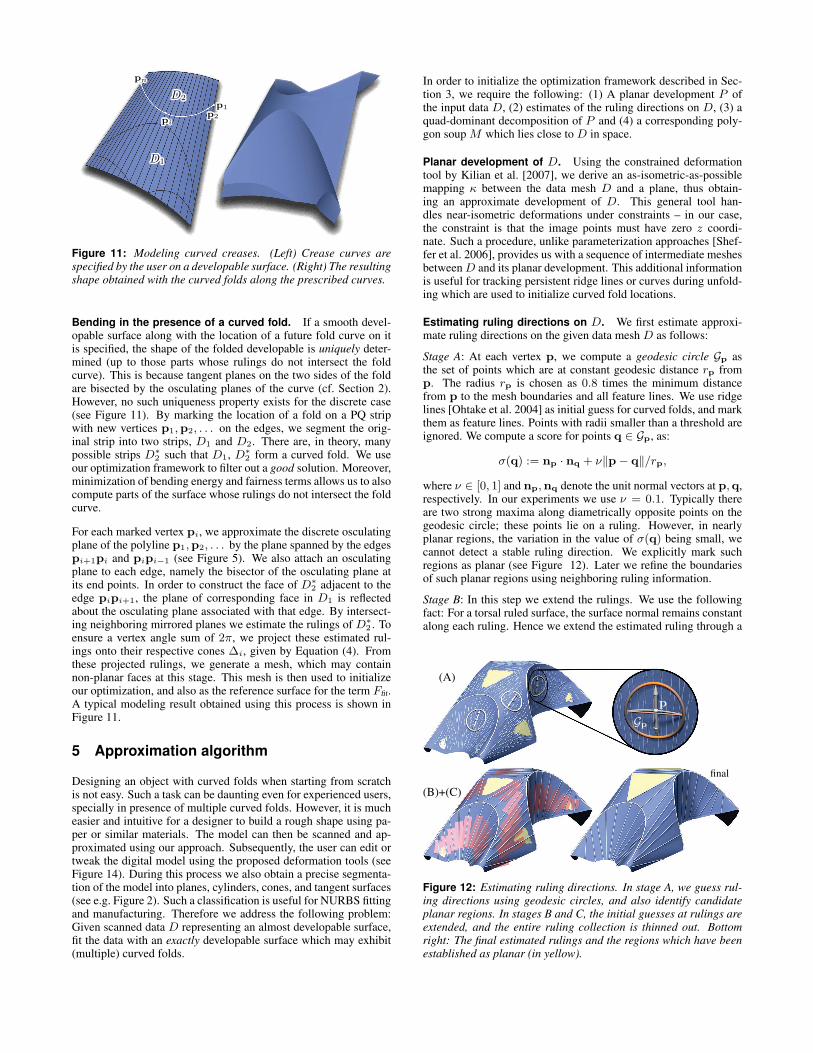
Figure 11: Modeling curved creases. (Left) Crease curves arespecified by the user on a developable surface. (Right) The resultingshape obtained with the curved folds along the prescribed curves.

Bending in the presence of a curved fold. If a smooth devel-opable surface along with the location of a future fold curve on itis specified, the shape of the folded developable is uniquely deter-mined (up to those parts whose rulings do not intersect the foldcurve). This is because tangent planes on the two sides of the foldare bisected by the osculating planes of the curve (cf. Section 2).However, no such uniqueness property exists for the discrete case(see Figure 11). By marking the location of a fold on a PQ stripwith new vertices p1,p2, . . . on the edges, we segment the orig-inal strip into two strips, D1 and D2. There are, in theory, manypossible strips D�

2 such that D1, D�2 form a curved fold. We use

our optimization framework to filter out a good solution. Moreover,minimization of bending energy and fairness terms allows us to alsocompute parts of the surface whose rulings do not intersect the foldcurve.

For each marked vertex pi, we approximate the discrete osculatingplane of the polyline p1,p2, . . . by the plane spanned by the edgespi+1pi and pipi− 1 (see Figure 5). We also attach an osculatingplane to each edge, namely the bisector of the osculating plane atits end points. In order to construct the face of D�

2 adjacent to theedge pipi+1, the plane of corresponding face in D1 is reflectedabout the osculating plane associated with that edge. By intersect-ing neighboring mirrored planes we estimate the rulings of D�

2 . Toensure a vertex angle sum of 2π, we project these estimated rul-ings onto their respective cones ∆i, given by Equation (4). Fromthese projected rulings, we generate a mesh, which may containnon-planar faces at this stage. This mesh is then used to initializeour optimization, and also as the reference surface for the term Ffit.A typical modeling result obtained using this process is shown inFigure 11.

5 Approximation algorithm

Designing an object with curved folds when starting from scratchis not easy. Such a task can be daunting even for experienced users,specially in presence of multiple curved folds. However, it is mucheasier and intuitive for a designer to build a rough shape using pa-per or similar materials. The model can then be scanned and ap-proximated using our approach. Subsequently, the user can edit ortweak the digital model using the proposed deformation tools (seeFigure 14). During this process we also obtain a precise segmenta-tion of the model into planes, cylinders, cones, and tangent surfaces(see e.g. Figure 2). Such a classification is useful for NURBS fittingand manufacturing. Therefore we address the following problem:Given scanned data D representing an almost developable surface,fit the data with an exactly developable surface which may exhibit(multiple) curved folds.

In order to initialize the optimization framework described in Sec-tion 3, we require the following: (1) A planar development P ofthe input data D, (2) estimates of the ruling directions on D, (3) aquad-dominant decomposition of P and (4) a corresponding poly-gon soup M which lies close to D in space.

Planar development of D. Using the constrained deformationtool by Kilian et al. [2007], we derive an as-isometric-as-possiblemapping κ between the data mesh D and a plane, thus obtain-ing an approximate development of D. This general tool han-dles near-isometric deformations under constraints – in our case,the constraint is that the image points must have zero z coordi-nate. Such a procedure, unlike parameterization approaches [Shef-fer et al. 2006], provides us with a sequence of intermediate meshesbetweenD and its planar development. This additional informationis useful for tracking persistent ridge lines or curves during unfold-ing which are used to initialize curved fold locations.

Estimating ruling directions on D. We first estimate approxi-mate ruling directions on the given data mesh D as follows:

Stage A: At each vertex p, we compute a geodesic circle Gp asthe set of points which are at constant geodesic distance rp fromp. The radius rp is chosen as 0.8 times the minimum distancefrom p to the mesh boundaries and all feature lines. We use ridgelines [Ohtake et al. 2004] as initial guess for curved folds, and markthem as feature lines. Points with radii smaller than a threshold areignored. We compute a score for points q 2 Gp, as:

σ(q) := np � nq + νkp− qk/rp,

where ν 2 [0, 1] and np,nq denote the unit normal vectors at p,q,respectively. In our experiments we use ν = 0.1. Typically thereare two strong maxima along diametrically opposite points on thegeodesic circle; these points lie on a ruling. However, in nearlyplanar regions, the variation in the value of σ(q) being small, wecannot detect a stable ruling direction. We explicitly mark suchregions as planar (see Figure 12). Later we refine the boundariesof such planar regions using neighboring ruling information.

Stage B: In this step we extend the rulings. We use the followingfact: For a torsal ruled surface, the surface normal remains constantalong each ruling. Hence we extend the estimated ruling through a

(A)

(B)+(C)

final

p

Gp

Figure 12: Estimating ruling directions. In stage A, we guess rul-ing directions using geodesic circles, and also identify candidateplanar regions. In stages B and C, the initial guesses at rulings areextended, and the entire ruling collection is thinned out. Bottomright: The final estimated rulings and the regions which have beenestablished as planar (in yellow).

point p until the surface normals in the end points deviate from thenormal np in p more than a pre-defined threshold. Rulings are alsoterminated if they come close to feature lines or boundaries. Forpurposes of later pruning, we assign the negative mean deviation ofsurface normals along the ruling from np as a measure of qualityto each extended ruling.

Stage C: The set of rulings obtained so far is thinned out whileretaining rulings with high quality measure. We use a greedy ap-proach: The ruling with highest quality measure is retained, and theones intersecting a narrow band around it are removed. Here it isimportant to find the right measure of proximity of rulings, becausethe surface may exhibit conical parts where rulings intersect at acommon vertex. Thus our band is shorter than the ruling and cen-tered in its midpoint (in Figure 12 (B+C) these bands are markedin red and slightly widened for better visibility). All other rulingswhich intersect this band are considered ‘close’ and are removed.

We continue the process of pruning until we get a set of (roughly)evenly spaced rulings on the surface. Regions marked as planar areconfirmed to be planar if they are bounded by three or more rulingsor boundary edges.

Quad dominant decomposition of P . After estimating andpruning the rulings, we now deal with initializing the planar de-velopment P of D.

We use the development mapping κ to map the estimated ruling di-rections from the surface D to the plane. From this set of mappedrulings, we generate a coarse quad-dominant mesh P . Note thathere a correct connectivity is much more important than the ac-tual coordinates of the vertices. Subsequent optimization retainsthe connectivity of the initial mesh while updating the vertex posi-tions.

The available input data for mesh generation are the estimated rul-ings mapped to the plane, the boundary of the planar mesh κ(D),and the location of ridge lines in the original surface, which areused as candidate curved fold locations (see Figure 13, left). First,all end points of rulings are snapped to the closest boundary orridge line — or, if the latter are too far away, are clustered in apoint. Additionally short ridge lines are contracted to a single conepoint (see Figure 13, center). Depending on the snapping target,we roughly classify an endpoint as boundary point, fold point, orcone point, respectively. In our examples, we frequently encoun-tered combinations of two of these (e.g. a curved fold might extendto the boundary). The extension of rulings to boundary and ridgelines might introduce intersections close to ruling end points. Suchintersections are resolved by swapping the corresponding end pointvertex coordinates. We get a preliminary mesh by connecting rul-ing end points as they are traversed along the boundary and ridgelines, generating mostly long quadrilateral faces.

Figure 13: Initial mesh layout. Left: A given collection of rulings(blue), ridge lines (brown), and mesh boundaries (gray). Center:Ruling endpoints are snapped and classified as boundary points(gray), fold points (blue) and cone points (brown). Right: By in-serting and deleting rulings, a valid mesh connectivity without T-junctions is obtained. The planar parts of the original shape aremarked in yellow.

The resulting mesh is next modified by deleting or inserting rulingsbased on the following observations: (i) From any point on a fold,two rulings must emanate to prevent any T-junctions on the fold.(ii) Planar regions must be bounded either by rulings or a boundarycurve. (iii) Boundary corner points should be included to preservethe shape of the base mesh. (iv) Faces adjacent to cone points mighthave more than four vertices. To ensure an optimal approximationof these regions, such faces need to be split into triangles or quadsfor our subdivision stage to apply. If a face holds more than a singlecone point and the connecting lines lie entirely in the face, rulingsare inserted connecting the cone points. If necessary, the faces orig-inating from this step are further split by inserting rulings emanat-ing from cone points. Finally, we obtain a quad dominant planarmesh P (see Figure 13, right).

Initialization of the polygon soup M . Initialization of our op-timization procedure is complete when a polygon soup M , corre-sponding to the development P and close to the original shape D,is found. We find a face M i of M corresponding to a face P i of Pby applying κ− 1 to the vertices of P i. Since the resulting vertices,in general, do not form a planar polygon which is isometric to P i,we register a copy of P i to these mapped vertices to initialize M i.

Now we can apply the optimization alogrithm of Section 3 and ob-tain a mesh which approximates the given data D and has the op-timized version of P as its precise development. In order to effi-ciently achieve high approximation quality, we start with a coarseapproximation which is subsequently refined (by splitting quads inruling direction) and optimized again. Results are shown in Figures1, 2, 7, 14 and 16.

6 Further applications and discussion

As illustrated by Figure 14, surface reconstruction can nicely becombined with deformation tools such as [Kilian et al. 2007]. Wefirst compute a digital reconstruction of a physical model and thenvary its shape by an as-isometric-as possible deformation. The de-formation will introduce deviations from a true developable surface,but it turns out that our reconstruction works very well on such de-formed data sets. Note that even precisely isometric deformationsin general do not preserve rulings and therefore rulings have to bere-estimated. In the example of Figure 14 it turned out that the op-timization worked well with the initialization for the reconstructionof the physical model. In other cases, one may have to re-initializefor intermediate positions in a deformation sequence.

We emphasize here that the design and reconstruction of objectswith curved folds is not simply solvable by a parameterizationmethod. Parameterization will not yield any information about theprecise location of folds, rulings and types of ruled patches, nor willit modify a data set to become precisely developable.

The nature of curved folds. Digital reconstruction of physicalpaper models yields a segmentation into torsal ruled patches. Thisprovides insight into the typical behavior of a developable surfacenear curved folds. Some frequently occurring situations are de-picted in Figure 2. In this way, our work can further contributeboth to the theory of curved folding and to applications, e.g., to thedevelopment of interactive CAD tools for modeling objects withcurved folds.

Architectural freeform structures. Developable surfaces areprominently visible in architectural design [Shelden 2002; Glaeserand Gruber 2007; Pottmann et al. 2007]. In particular, Frank O.Gehry has been using these surfaces quite extensively. The pres-ence of rulings simplifies the actual construction. Panelization, e.g.

Figure 14: A bending sequence which exhibits a curved fold. The left hand mesh is the result of approximating a 3D scan of a paper model.The other shapes have been computed by combining our reconstruction algorithm with an as-isometric-as possible shape modification of thereference surface, i.e., the reference data set in Ffit has changed, but the remaining data for optimization are taken from the left hand mesh.

by metal tiles, is easy due to developability. The aesthetic contin-uation of a tiling over a general sharp edge is a difficult problem.However, at a curved fold the tile continuation is optimal (cf. Fig-ures 1 and 15) and the design of the tiling can be done in the devel-opment. Note that our segmentation into torsal ruled patches is ofhigh importance for manufacturing such architectural structures.

Industrial design. The shapes shown in our paper hopefully pro-vide a first impression of the wide applicability of curved foldingin industrial design. Such applications may require a high qual-ity NURBS representation which is very easy to compute from oursegmentation into torsal ruled patches. The exact locations of rul-ings (which cannot be seen in the triangle mesh of a 3D scan ofa physical model) are important for manufacturing as well. More-over, due to the fairness measures in our optimization frameworkwe obtain aesthetically pleasing digital models while maintainingthe hard constraint of a precise planar development.

Limitations. We performed a large number of experiments ondata sets obtained by scanning models built from fabric or materi-als with a similar stretching behavior. It turned out that these mod-els hardly behave like developable surfaces, particularly in regionswith drastic folds. Hence, we must leave the task of (roughly) ap-proximating such data by a single developable surface with curvedfolds to future research. The fully automatic generation of the ini-tial planar mesh P worked well for all considered models. The onlyexception was the car model, a significantly more complex model,where we interactively modified a few ruling directions to ensure asuitable mesh for the adaptive subdivision we employ.

Implementation and run times. In our current implementationwe use CHOLMOD [Davis and Hage 2001] to solve a sparse linearsystem and the KNITRO optimization package for constrained non-linear optimization. Average runtimes for the models of Figure 16

Figure 15: Architectural design that features rulings as part of thesupport structure.

are 160 seconds for ruling extraction (on 50K reference mesh), 20seconds mesh layout and 140 seconds for optimization. The objec-tive function was reduced to order of 10− 4. In particular the vertexagreement term is less than 10 − 4. The fitting weight λ was reducedby a factor of 0.1 after each step of subdivision to favor fair solutionsurfaces instead of best approximating ones.

Conclusion and Future research. We presented a computa-tional framework for the design and digital reconstruction of de-velopable surfaces with curved folds. Our work contributes to thediscrete differential geometry of developable surfaces, to the dis-crete geometry of curved folds, and to the geometric optimizationof surfaces with curved folds. Moreover, we illustrated the potentialof our developments on a number of examples motivated by appli-cations in architecture, industrial design and manufacturing. Giventhe limited amount of prior research in this area, there is still a lotof work to be done. Open problems include the reconstruction ofmodels where a high approximation error has to be admitted such asscanned fabric, a careful analysis and classification of typical ruledpatch arrangements at curved folds, and the development of novelinteractive modeling tools for curved folding.

Acknowledgments. This work is supported by the Austrian Sci-ence Fund (FWF) under grants S92 and P18865. Niloy is also sup-ported by a Microsoft outstanding young faculty fellowship. Weare grateful to Heinz Schmiedhofer for his help with building andscanning the paper models and rendering the reconstructed mod-els. We also thank Martin Peternell and Johannes Wallner for theirthoughtful comments on the subject.

References

AUMANN, G. 2004. Degree elevation and developable Bezier surfaces.Comp. Aided Geom. Design 21, 661–670.

BO, P., AND WANG, W. 2007. Geodesic-controlled developable surfacesfor modeling paper bending. Comp. Graphics Forum 26, 3, 365–374.

BOBENKO, A., AND SURIS, Y., 2005. Discrete differential geometry.Consistency as integrability. Preprint, http://arxiv.org/abs/math.DG/0504358.

BOTSCH, M., PAULY, M., GROSS, M., AND KOBBELT, L. 2006. Primo:coupled prisms for intuitive surface modeling. In Symp. Geom. Process-ing, 11–20.

CERDA, E., CHAIEB, S., MELO, F., AND MAHADEVAN, L. 1999. Conicaldislocations in crumpling. Nature 401, 46–49.

CERDA, E., MAHADEVAN, L., AND PASINI, J. M. 2004. The elements ofdraping. Proc. Nat. Acad. Sciences 101, 7, 1806–1810.

CHU, C. H., AND SEQUIN, C. 2002. Developable Bezier patches: proper-ties and design. Comp.-Aided Design 34, 511–528.

DAVIS, T. A., AND HAGE, W. W. 2001. Multiple-rank modifications ofa sparse cholesky factorization. SIAM Journal on Matrix Analysis andApplications 22, 4, 997–1013.

Figure 16: A gallery of digi-tal paper models. Models werecomputed with the algorithm de-scribed in Section 5 with scans ofreal paper models as referencesurfaces. Reconstructed mod-els exhibit curved and straightfolds and can be isometricallyunfolded into the plane. Severalspecial cases like cone singular-ities (top row – middle) and con-verging curved folds (top row –right) are shown.

DEMAINE, E., AND O’ROURKE, J. 2007. Geometric Folding Algorithms:Linkages, Origami, Polyhedra. Cambridge Univ. Press.

DESBRUN, M., POLTHIER, K., AND SCHRODER, P. 2005. Discrete Dif-ferential Geometry. Siggraph Course Notes.

DO CARMO, M. 1976. Differential Geometry of Curves and Surfaces.Prentice-Hall.

FREY, W. 2004. Modeling buckled developable surfaces by triangulation.Comp.-Aided Design 36, 4, 299–313.

GLAESER, G., AND GRUBER, F. 2007. Developable surfaces in contem-porary architecture. J. of Math. and the Arts 1, 1–15.

HUFFMAN, D. A. 1976. Curvature and creases: a primer on paper. IEEETrans. Computers C-25, 1010–1019.

JULIUS, D., KRAEVOY, V., AND SHEFFER, A. 2005. D-charts: Quasi-developable mesh segmentation. Computer Graphics Forum 24, 3, 581–590. Proc. Eurographics 2005.

KERGOSIEN, Y., GOTUDA, H., AND KUNII, T. 1994. Bending and creas-ing virtual paper. IEEE Comp. Graph. Appl. 14, 1, 40–48.

KILIAN, M., MITRA, N. J., AND POTTMANN, H. 2007. Geometric mod-eling in shape space. ACM Trans. Graphics 26, 3, 64.

LIU, Y., POTTMANN, H., WALLNER, J., YANG, Y.-L., AND WANG, W.2006. Geometric modeling with conical meshes and developable sur-faces. ACM Trans. Graphics 25, 3, 681–689.

MASSARWI, F., GOTSMAN, C., AND ELBER, G. 2006. Papercraft modelsusing generalized cylinders. In Pacific Graph., 148–157.

MITANI, J., AND SUZUKI, H. 2004. Making papercraft toys from meshesusing strip-based approximate unfolding. ACM Trans. Graphics 23, 3,259–263.

OHTAKE, Y., BELYAEV, A., AND SEIDEL, H.-P. 2004. Ridge-valley lineson meshes via implicit surface fitting. ACM Trans. Graph. 23, 3 (Au-gust), 609–612.

PEREZ, F., AND SUAREZ, J. A. 2007. Quasi-developable B-spline surfacesin ship hull design. Comp.-Aided Design 39, 853–862.

PETERNELL, M. 2004. Developable surface fitting to point clouds. Comput.Aided Geom. Des. 21, 8, 785–803.

POTTMANN, H., AND WALLNER, J. 2001. Computational Line Geometry.Springer.

POTTMANN, H., HUANG, Q.-X., YANG, Y.-L., AND HU, S.-M. 2006.Geometry and convergence analysis of algorithms for registration of 3Dshapes. Int. J. Computer Vision 67, 3, 277–296.

POTTMANN, H., ASPERL, A., HOFER, M., AND KILIAN, A. 2007. Ar-chitectural Geometry. Bentley Institute Press.

ROSE, K., SHEFFER, A., WITHER, J., CANI, M.-P., AND THIBERT, B.2007. Developable surfaces from arbitrary sketched boundaries. InSymp. Geometry Processing. 163–172.

SAUER, R. 1970. Differenzengeometrie. Springer.

SHATZ, I., TAL, A., AND LEIFMAN, G. 2006. Papercraft models frommeshes. Vis. Computer 22, 825–834.

SHEFFER, A., PRAUN, E., AND ROSE, K. 2006. Mesh parameterizationmethods and their applications. Found. Trends. Comput. Graph. Vis. 2,2, 105–171.

SHELDEN, D. 2002. Digital surface representation and the constructibilityof Gehry’s architecture. PhD thesis, M.I.T.

SUBAG, J., AND ELBER, G. 2006. Piecewise developable surface approx-imation of general NURBS surfaces with global error bounds. In Proc.Geometric Modeling and Processing. 143–156.

WANG, C., AND TANG, K. 2004. Achieving developability of a polygonalsurface by minimum deformation: a study of global and local optimiza-tion approaches. Vis. Computer 20, 521–539.

WANG, C. C. L. 2008. Towards flattenable mesh surfaces. Comput. AidedDes. 40, 1, 109–122.

WERTHEIM, M. 2004. Cones, Curves, Shells, Towers: He Made PaperJump to Life. The New York Times, June 22.

YAMAUCHI, H., GUMHOLD, S., ZAYER, R., AND SEIDEL, H.-P. 2005.Mesh segmentation driven by Gaussian curvature. Vis. Computer 21,659–668.