Current Measurement UsingAcoustic Doppler Current Profilers

Synopsis Principles of operation

Types of instruments: Narrowband, Broadband

Shipboard systemsAncillary measurements, calibration

Moored Instruments

Other applications Acoustic backscatter, Waves, Wind …

Gwyn Griffiths 2004

email: gxg@soc.soton.ac.uk web: http://www.soc.soton.ac.uk/OED/gxg

ADCP Applications

Acoustic scatterersoce

an

explo

rer.

noaa.g

ov

Pteropod, Limacina sp.

Myctophid fish, Benthosema pterotumKrill, Euphausia superba

scri

pp

snew

s.ucs

d.e

d

u

Copepod, Calanus sp.

Physonect Siphonophore,

Marrus orthocanna

oce

an

explo

rer.

noaa.g

ov

Acoustic backscatter in the ocean

t

Sv (dB.m-1)

Principle of operationR

D I

nstr

umen

ts

€

Δf =2 f txv

csinθ Where is the angle of

the beam to the vertical

Range gating: at time t after start of transmission of a pulse of duration the return echo is from a distance:

€

l2 =c.(t +τ )

2

€

l1 =c.t

2 and at a time later from

a distance and so in space, the range bin separation is:

€

Δl =c.τ

2

Range resolution

0

1

2

3Range

0 1 2 3time0

t

Resolution in range is somewhat different to the separation of range bins

Instead, the resolution is determined by the convolution of the transmit pulse envelope and the receiver window - both are usually the same rectangular functions:

€

z t( ) = x−∞

∞

∫ t'( )y t − t'( )dt'

€

y t − t'( ) is

€

y t( ) folded backwards

and slid pastwith the convolution being the area of the product, which is a triangle, with an extent of , or a distance of c.

€

x t'( )x(t)

time

wBin4

3

2

1

Adapted from RDI Broadband primer

Narrowband and BroadbandNumber of independent samples of a signal in time isgiven by the time bandwidth product .ΔB

For a simple rectangular pulse of a single frequency:

ΔB = 1/ so, number of independent samples is 1 = Narrowband

Bandwidth is increased by using a chirp within the pulse, let

ΔB = 16/ hence the number of independent samples is 16This is what could be used in a Broadband ADCP

Single tone

Chirp

Single-ping velocity variance is:

€

2 = k.c 2

f 2 .τ 4ΔB2 sin2 θ Frequency (kHz)Bin length (m)

1200 600 300

1 3 12 6 23 13 552 2 6 3 11 6 274 - 3 2 6 3 14

Standard deviation in cm/s

Black - Broad

Red - Narrow

Profiling rangeThe received signal strength varies as:

RSSI = SL + SV -20 log(R) - 20 log(R) + 20 log(R) -2R +K

where SL is the transmit source level (dB rel. 1Pa at 1 m) SV is the mean volume backscatter strength (dB rel m-1) R is the range along the beam (m) is the sound absorption coefficient (dB.m-1) K is an instrument and frequency specific ‘constant’

Outgoing spherical spreading

Incoming spherical spreading

Increasedscatteringvolume

Shipboard ADCPs

Histograms of the depth obtained with the OS‑75 on station based on a criterion of 50%-good in each ensemble. Only 5 out of 67 observations achieved less than the manufacturer’s specification of 650 m.

Examples on RRS Discovery : RD Instruments 150 kHz NarrowBand and 75 kHz Ocean Surveyor

RD

Ins

trum

ents

Transducer installed on Discovery, with fence to prevent bubbles at transducer face

Bottom track

-60

-50

-40

-30

-20

-10

0

Transducer response (dB)

-40 -20 0 20 40Angle (˚)

0

50

100

150

200

250

Depth (m)

-50 -40 -30 -20 -10 0

Received signal (dB)

Same principles as water track Longer transmit pulse & receiver window, give reduced velocity

variance, ensure bottom is completely insonified Transducer beam pattern affects shape of bottom echo and

maximum profiling distance, ~ depth * cos (), typically 30˚ Algorithms for bottom detection consider rate of rise as well as

absolute signal levels.

Bottom depth=230m

Heading accuracyN

Vs

E()

Static Gyrocompass error G (˚) given by (Bowditch, 1977):

G = 0.327 S cos (C) sec (L)

where S is the speed in m.s-1, C the course (˚) and L the latitude (˚)Dynamic errors due to Schüler oscillation also degrade performanceEstimate Gyro error using independent system such as Carrier Phase GPS

Gyrocompass error on Discovery 198, south of 60˚S (Griffiths, 1994)

Heading error produces a spurious cross-track current of Vs.sin () This would be 8.7 cm.s-1 for = 1˚ at a speed of 5 m.s-1

Dashed lines are +/- one standard deviation

Gyro error in practice

At 77˚ 36’ NAugust 2004 ~ 3˚ gyro error

84 minute time constantShip moving to ship steady

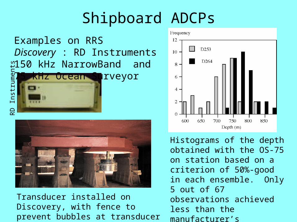
Merging ADCP with navigation data

5-minute averaged ADCP ensembles, overlayed with 2-minute averaged ship-over-ground from differentiated GPS positions 1 s apart.

Temperature=15.8˚C

A = 1.021

= -1.69˚i.e. Rotate ADCP readings ACW to match GPS

bottomew, bottomns are ADCP bottom track datave, vn are corresponding GPS-derived ship data3DF GPS heading correction has been applied

Data from RRS James Clark Ross, JR106 on the north Icelandic shelf, August 2004.

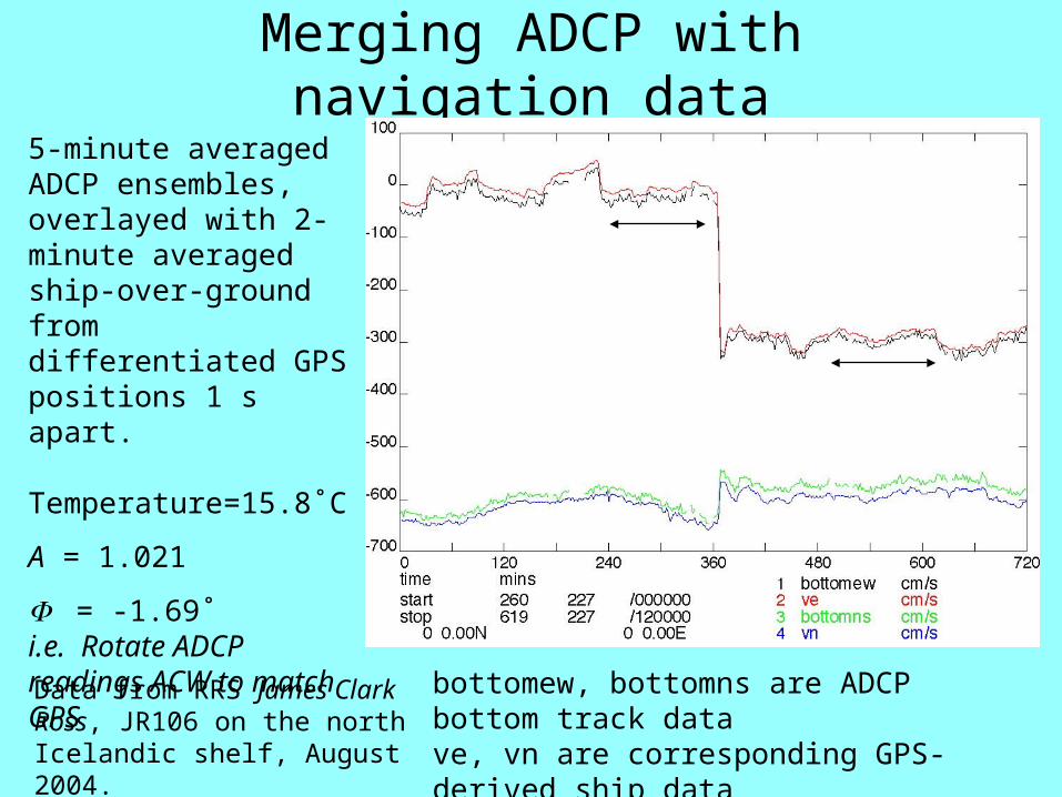
Water-track calibrationUsed when bottom track calibration not possible

TechniqueSolve for the Amplitude scaling factor A and the offset angle from a set of measurements made on a zig-zag course, assuming that local currents on a zig-zag are steady.

Let dvd and dud be the difference in ADCP velocity components before and after the turn and dus and dvs the difference in the ship velocity components, then Pollard and Read (1989) showed that:

€

φ=arctandvd .dus − dud .dvs

dvd .dvs + dud .dus

⎛

⎝ ⎜

⎞

⎠ ⎟

€

A = −dvd .dvs + dud .dus

cos(φ).(dud2 + dvd

2 )

⎛

⎝ ⎜

⎞

⎠ ⎟

ADCP measurements of a gyre in the Alboran SeaF

rom

All

en a

t al.

(199

7) s

ee n

otes

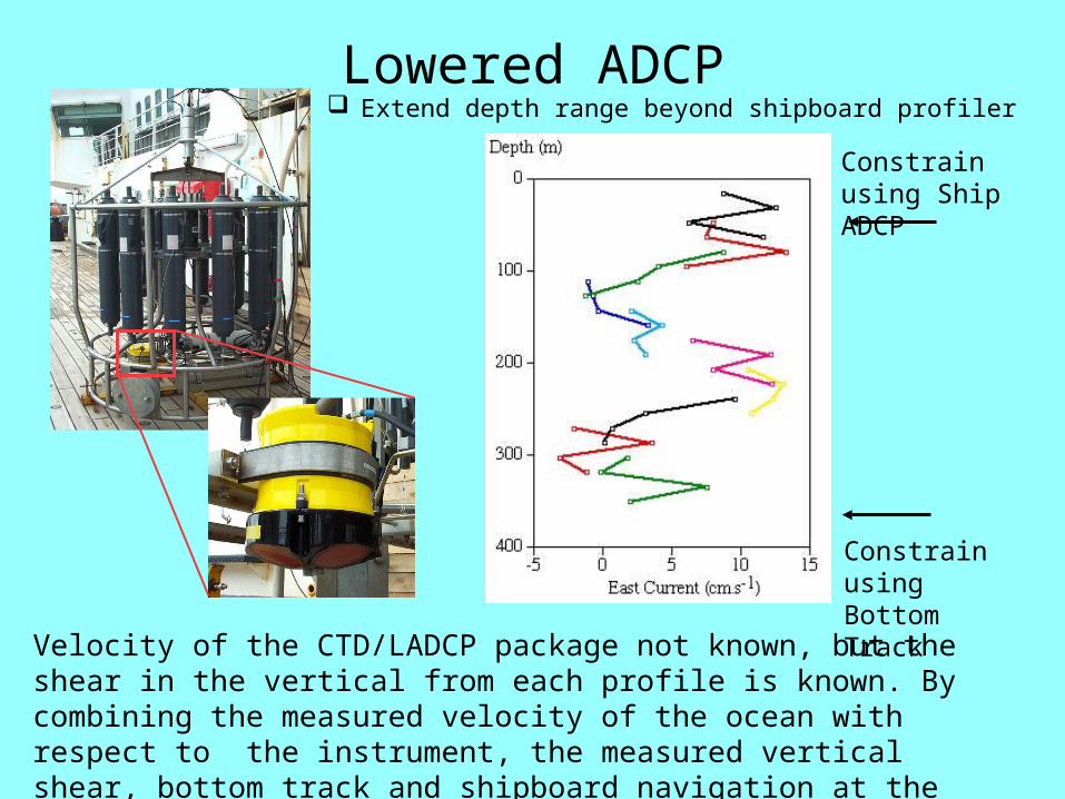
Lowered ADCP Extend depth range beyond shipboard profiler

Velocity of the CTD/LADCP package not known, but the shear in the vertical from each profile is known. By combining the measured velocity of the ocean with respect to the instrument, the measured vertical shear, bottom track and shipboard navigation at the start and end of the station, absolute velocity profiles are

obtained.

Constrain using Ship ADCP

Constrain using Bottom Track

Moored ADCPsMonitoring the Faroe-Shetland and Faroe Bank Channels

Hansen et al.www.gfi.uib.no/forskning/nwoce/pdf-filer/h_out262.pdf

Acoustic backscatter in the Strait of Gibraltar

Vertical velocity in the Strait of Gibraltar

Biological information from an ADCP

RDI VM-150 ADCPDiscovery 224 December 19964 m bins 2 minute ensembles

Wind information from an ADCP

From Zedel (2001)

Figure 4(a) Scatterplot between wind speed observed at Argentia and ADCP intensity levels at mooring P718

Wave information from an ADCP

From http://www.frf.usace.army.mil/capefear/realtime.stm

ADCP Bibliography 2004Gwyn Griffiths, SOC email gxg@soc.soton.ac.uk

General

Gordon, R.L., 1996. ADCP Principles of operation - a practical primer. 2nd edition, RD Instruments document P/N 951-6069-00.Plueddemann, A., 2001. Profiling Current Meters. In Encyclopedia of Ocean Science, J Steele, S Thorpe and K Turekian (eds.), London, Academic Press.

Backscatter from animals

Stanton, T.K., Chu, D. and Wiebe, P. H., Martin, L.V. and Eastwood, R.L., 1998a. Sound scattering by several zooplankton groups.I. Experimental determination of the dominant scattering mechanisms. J. Acoust. Soc. Am., 103:225-235.Stanton, T. K., Chu, D. and Wiebe, P. H. (1998b) Sound scattering by several zooplankton groups. Part II Scattering models. J. Acoust. Soc. Am., 103: 236-253.

Vessel mounted ADCP performance

N P Holliday, R T Pollard and G Griffiths, 2003. A comparison of simultaneous measurements from shipboard VM-150 and OS-75 acoustic Doppler current profilers. Proceedings 7th IEEE Working Conference on Current Measurement, San Diego, March 2003. Piscataway: IEEE, pp. 191-196.

Navigation errors and use of 3D GPS

Bowditch N. (1977) American Practical Navigator, Volume I. Defense Mapping Agency Hydrographic Center, 1386pp.

Griffiths G. 1994 Using 3D GPS heading for improving underway ADCP data, J Atmospheric and Oceanic Technology, Vol. 11, No.4, pp 1135-1143.Ruiz, S., Font, J., Griffiths, G. and Castellon, A., 2002. Estimation of heading gyrocompass error using a GPS 3DF system: impact on ADCP measurements. Scientia Marina, 66(4): 347-54,

Pollard, R. T. & Read, J. 1989 A method of calibrating ship-mounted acoustic Doppler profilers and the limitations of gyro compasses.Journal of Atmospheric and Oceanic Technology, 6(6), 859-865.Examples of shipboard ADCP data

Data from Upper Ocean underway operations on BIO Hesperides cruise OMEGA-ALGERS (cruise 36) using SeaSoar and ADCP30/9/96 - 14/10/96   J. T. Allen, D.A. Smeed, N. Crisp, S. Ruiz, S. Watts, P. J. Velez, P. Journet, O. Rius and A. Castellón, available at http://www.soc.soton.ac.uk/GDD/omega/Hesp/Doc17.html

Lowered ADCP

Visbeck, Martin, 2002: Deep Velocity Profiling Using Lowered Acoustic Doppler Current Profilers: Bottom Track and Inverse Solutions Journal of Atmospheric and Oceanic Technology : Vol. 19, No. 5, pp. 794–807.

Example of moored ADCP data

Hansen et al., http://www.gfi.uib.no/forskning/nwoce/pdf-filer/h_out262.pdf

Biological applications of ADCPs

Griffiths, G., Fielding, S. and Roe, H.S.J., 2002. Biological-Physical-Acoustical Interactions. Chapter 11 in ‘The Sea, Volume 12: Biological-Physical Interaction’, eds. A. R. Robinson, J. J. McCarthy and B. J. Rothschild. J Wiley and Sons, New York, pp. 441-474.

Roe, H.S.J. & Griffiths, G. 1993 Biological information from an ADCP, Marine Biology, 115 (2), 339-346.

Roe, H S J, Griffiths, G, Hartman, M, Crisp, N., 1996 Variability in biological distributions and hydrography from concurrent Acoustic Doppler Current Profiler and SeaSoar surveys. ICES Journal of Marine Science, 53: 131-138.

Fielding, S., Griffiths, G. and Roe, H. S. J., Biological validation of ADCP acoustic backscatter through direct comparison with net samples and model-predictions based on acoustic backscatter models. ICES Journal of Marine Science, 61: 184-200.

Using ADCPs to estimate winds and waves

Zedel, L., 2001: Using ADCP Background Sound Levels to Estimate Wind Speed. Journal of Atmospheric and Oceanic Technology, 18, 1867-1881.

U.S. Army Corps of Engineers http://www.frf.usace.army.mil/capefear/realtime.stm for live ADCP waves data