Embed Size (px)
Citation preview

u n i ve r s i t y o f co pe n h ag e n
Sensitivity enhancement in solid-state magic-angle spinning NMR spectroscopy
Novel decoupling schemes and dipolar-driven spin-state selection
Vinther, Joachim Møllesøe
Publication date:2012
Document versionEarly version, also known as pre-print
Citation for published version (APA):Vinther, J. M. (2012). Sensitivity enhancement in solid-state magic-angle spinning NMR spectroscopy: Noveldecoupling schemes and dipolar-driven spin-state selection.
Download date: 13. Aug. 2021

Sensitivity enhancement in solid-state
magic-angle spinning NMR spectroscopy
Novel decoupling schemes and dipolar-driven spin-state
selection
Joachim Møllesøe Vinther
Ph.D. Thesis
Supervisor: Niels Chr. Nielsen
Interdisciplinary Nanoscience Center (iNANO)and
Department of ChemistryAarhus University
2012

ii

Abstract
Two main research areas are covered by this thesis which describe pulsesequence development for magic-angle spinning (MAS) solid-state nuclearmagnetic resonance (NMR): Resolution enhancement by dipolar-driven spin-state-selective excitation and refocused continuous-wave heteronuclear de-coupling.
Analytically and Optimal Control-based dipolar-driven spin-state selec-tive excitation schemes are presented as means of avoiding line broadening inMAS solid-state NMR spectra of carbonyl resonances due to the scalar cou-pling to the α-carbon in 13C-labelled samples. The analytically developedpulse sequences combine dipolar-recoupling elements of dierent recouplingconditions in order to obtain spin-state selection. Correspondence betweenanalytically obtained results, simulations, and experimental results are pre-sented and further improvements for general applicability are proposed. TheOptimal Control-based sequences show a remarkable eciency reaching thetheoretical transfer bounds in simulations and close to this experimentally.The sequences, however, depends on the spin-system geometry and futureguidelines for achievement of general applicable sequences are outlined.
Refocused continuous-wave (rCW) decoupling is presented as an e-cient and robust means of decoupling abundant spins in order to obtainhigh-resolution MAS solid-state NMR spectra of low-γ (gyromagnetic ra-tio) nuclei. The scheme is developed through a thorough average Hamil-tonian analysis of CW decoupling and thereof derived incorporation of av-eraging refocusing-pulses. The rCW sequences show state-of-the-art de-coupling performance combined with stability towards rf-amplitude varia-
iii

iv Abstract
tions, -frequency osets, and -inhomogeneity as well as robustness on a verywide range of chemical shift anisotropies. The sequences are introduced asmeans of proton decoupling, however, the robustness towards chemical shiftanisotropy makes rCW suitable for uorine-19 decoupling, for which state-of-the-art decoupling performance is presented. Furthermore, very eectivedecoupling in diluted spin systems is demonstrated. Together with easeof application and optimisation, rCW is ideal for low-sensitivity samples,where thorough optimisation of decoupling schemes are rendered impossible.These characteristics makes the rCW sequences broadly applicable.

Resumé
To hovedområder inden for magic-angle spinning (MAS) faststof kernemag-netisk resonans (NMR) pulssekvensudvikling er beskrevet i denne afhand-ling: Dipolkoblingsmedieret spin-state selektion til forbedring af den spek-trale opløsningsevne samt Refocused continuous-wave heteronuklear dekob-ling.
Linjeforbredningen af carbonyl-resonanser pga. den skalare kobling tilnabo-carbonatomet i 13C-mærkede forbindelser i MAS faststof NMR spek-tra adresseres vha. analytisk og Optimal Control-baserede protokoller tildipolkoblingsmedieret spin-state selektiv eksitation. I den analytisk ud-viklede pulssekvens kombineres dipolære rekoblingselementer med forskel-lige rekoblingsbetingelser for at opnå den ønskede spin-state selektion. Over-ensstemmelse mellem analytiske resultater, simuleringer og eksperimentelledata eftervises og endvidere beskrives forbedringstiltag, der vil gøre sekven-sen generelt anvendelig. Pulssekvenserne baseret på numeriske optimeringerviser eektiviteter på linie med de teoretiske maksima jf. simuleringer oghenved det samme eksperimentelt. Imidlertid afhænger disse sekvenserseekt kraftigt af spinsystemets geometri og videreudviklingen af disse måbaseres på et bredere sæt af spinsytemsparametre.
Den udviklede dekoblingssekvens, Refocused continuous-wave (rCW),viser en høj og robust dekoblingseektivitet under anvendelse som hetero-nuklear dekobling under optagelse af MAS faststof NMR spektra af kernermed lavt gyromagnetisk forhold. Protokollen er udviklet vha. en average-Hamilton-analyse af CW-dekobling, hvorved tilføjelse af refokuse-ringspulseviste sig at kunne udmidle de uønskede average Hamilton-operatorer. rCW
v

vi Resumé
sekvenserne udviser dekoblingseektiviteter på linie med state-of-the-artdekoblingssekvenser kombineret med stabilitet over for rf-amplitudevaria-tioner, -frekvensoset og -feltinhomogeniteter samt robusthed mht. kemiskskiftanisotropi. Sekvenserne introduceres i form af protondekobling, imid-lertid gør robustheden over for kemisk skiftanisotropi dem egnede til uor-19 dekobling, for hvilken state-of-the-art dekoblingseektivitet er eftervist.Hertil kommer, at rCW sekvenserne udviser enddog meget stor dekob-lingseektivitet i spin-fortyndede prøver. Disse karakteristika kombineretmed en let opsætning og en hurtig optimering af sekvenserne gør rCWmeget bredt anvendelig.

Acknowledgements
First of all I would like to thank my supervisor Niels Chr. Nielsen forintroducing me to the exciting topic of solid-state NMR pulse sequencedevelopment and knowledgeable supervision.
I thank Morten Bjerring for a lot of help with the spectrometers, otherpractical stu and many good answers on NMR questions. I would likewisethank Anders Bodholt Nielsen for teaching me solid-state NMR experimen-tal work practise, tips and tricks and Lasse Arnt Straasø for fruitful theo-retical discussions and for all the thoughtful answers and advises; and bothfor fantastic company. Furthermore, I thank all of the BioNMR group andmy oce colleges for the giving learning environment and good company.
I am pleased to thank Arno Kentgens and Ernst R. H. van Eck for host-ing my two stays at their NMR Laboratory in Nijmegen, The Netherlands,for corporation on setting-up and testing of decoupling sequences on theirstate-of-the-art 850 MHz spectrometer equipped with a 1.2 mm probe andon their home-build µMAS probe which made acquisition of valuable datafor publication possible.
I am also pleased to thank Navin Khaneja, Harvard University, Cam-bridge, Massachusetts, United States for inspiration and collaboration onthe work of development of decoupling sequences.
A special thank is directed to Ellen Møllesøe, Bo Møllesøe Vinther, andLasse Arnt Straasø for proofreading parts of the thesis.
Many thanks to my supportive family and to my lovely girlfriend Mariawho always supports me especially when it is most needed!
vii

viii Acknowledgements

Contents
Abstract iii
Resumé v
Acknowledgements vii
List of abbreviations xiii
1 Introduction 1
1.1 Sensitivity enhancement . . . . . . . . . . . . . . . . . . . . 31.1.1 Resolution enhancement . . . . . . . . . . . . . . . . 31.1.2 Intensity enhancement . . . . . . . . . . . . . . . . . 4
2 Magic-angle spinning solid-state NMR 7
2.1 Equation of motion and solutions . . . . . . . . . . . . . . . 72.2 Transformations . . . . . . . . . . . . . . . . . . . . . . . . . 102.3 Sample spinning . . . . . . . . . . . . . . . . . . . . . . . . 142.4 The interactions . . . . . . . . . . . . . . . . . . . . . . . . 14
2.4.1 The chemical shift . . . . . . . . . . . . . . . . . . . 152.4.2 The scalar coupling . . . . . . . . . . . . . . . . . . . 162.4.3 The dipolar coupling . . . . . . . . . . . . . . . . . . 17
3 Resolution enhancement by dipolar-driven spin-state selec-
tion 19
ix

x CONTENTS
3.1 Analytical dipolar-driven spin-state selection . . . . . . . . . 213.1.1 Exponentially modulated recoupling . . . . . . . . . 223.1.2 Dipolar-driven spin-state-selection . . . . . . . . . . 27
3.2 Numerical dipolar-driven spin-state selection . . . . . . . . . 383.2.1 Optimal Control . . . . . . . . . . . . . . . . . . . . 383.2.2 Optimal control based spin-state selection . . . . . . 39
3.3 Conclusion and perspectives . . . . . . . . . . . . . . . . . . 51
4 Refocused continuous-wave decoupling 55
4.1 Average Hamiltonian for continuous-wave decoupling . . . . 584.2 Refocused continuous-wave decoupling . . . . . . . . . . . . 71
4.2.1 Refocusing pulses . . . . . . . . . . . . . . . . . . . . 714.2.2 Phase modulation . . . . . . . . . . . . . . . . . . . 734.2.3 Purging pulses . . . . . . . . . . . . . . . . . . . . . 74
4.3 Performance comparisons . . . . . . . . . . . . . . . . . . . 754.4 Discussion and conclusion . . . . . . . . . . . . . . . . . . . 85
5 Fluorine decoupling by refocused continuous-wave 87
5.1 Refocused continuous-wave decoupling . . . . . . . . . . . . 885.2 Conlusion . . . . . . . . . . . . . . . . . . . . . . . . . . . . 95
6 Conclusions and perspectives 97
Bibliography 101
A Design of spin systems for simulations 113
A.1 Conventions and conversions . . . . . . . . . . . . . . . . . . 114A.2 Calculation of Euler angles . . . . . . . . . . . . . . . . . . 116A.3 Visualising the spin system . . . . . . . . . . . . . . . . . . 117A.4 The applied spin systems . . . . . . . . . . . . . . . . . . . 118
A.4.1 Resolution enhancement . . . . . . . . . . . . . . . . 119A.4.2 Proton decoupling . . . . . . . . . . . . . . . . . . . 122A.4.3 Fluorine decoupling . . . . . . . . . . . . . . . . . . 124

CONTENTS xi
B Experimental details 127
B.1 Sample preparation . . . . . . . . . . . . . . . . . . . . . . . 127B.2 Setting up experiments on the spectrometer . . . . . . . . . 127
B.2.1 General procedure . . . . . . . . . . . . . . . . . . . 128B.2.2 Special components . . . . . . . . . . . . . . . . . . . 129
B.3 Extracting spectral data . . . . . . . . . . . . . . . . . . . . 129
C Tabulated amplitude and phase of S3E waves shown section
3.2 131
D Publications 137
D.1 Refocused continuous-wave decoupling: A new approach toheteronuclear dipolar decoupling in solid-state NMR spec-troscopy . . . . . . . . . . . . . . . . . . . . . . . . . . . . . 137
D.2 Robust and Ecient 19F Heteronuclear Dipolar Decouplingusing Refocused Continuous-Wave Rf Irradiation . . . . . . 155

xii CONTENTS

List of abbreviations
γ gyromagnetic ratio
AHT average Hamiltonian theory
BCH BakerCampbellHausdor
CP Cross Polarisation
CS crystal xed system
CSA chemical shift anisotropy
D dipolar coupling
DARR Dipolar Assisted Rotational Resonance
EXPORT EXPonentially mOdulated Recoupling experimenT
FID free-induction decay
FWHM full width at half maximum
INADEQUATE Incredible Natural Abundance Double Quantum Trans-fer Experiment
IPAP in-phase anti-phase
J scalar coupling
xiii

xiv CONTENTS
LS laboratory system
MAS magic-angle spinning
NMR nuclear magnetic resonance
OC Optimal Control
PAS principal axis system
RADAR Rotor Assisted DipolAr Refocusing
rf radio frequency
RS rotor system
S3 spin-state selective
S3CT spin-state selective coherence transfer
S3E spin-state selective excitation
S/N signal-to-noise ratio
SH3 Src-homology 3
SPINAL small phase incremental alternation
TPPM two pulse phase modulation
XiX x-inverse-x

Chapter 1
Introduction
Contrary to liquid-state NMR, where resolution of 1 Hz (i.e. 1 Hz linewidths) is achievable, solid-state NMR still struggles with severe overlap-ping of resonances even in higher dimensional spectra. This discrepancystems from the anisotropic interactions of and between the nucleic spins.Anisotropic interaction will, to a great extent, be averaged by fast motionof the molecules (as compared to the time scale of the interactions), and inliquid-state NMR the interactions are averaged by the rotational motion ofthe molecules in solution. In solid-state NMR a completely dierent pictureis drawn. The molecules, either in a powder or single-crystal, are locked intheir positions and no or little averaging of the interactions takes place andas a starting point the line width is several kHz. The dierences are exempli-ed by simulated liquid- and solid-state spectra under dierent conditions,gure 1.1. The origin of these line width and the dierent interactions willbe discussed in chapter 2.
During the years many techniques have been invented and applied tocircumvent the inherent problem of line width in solid-state NMR which isnot only problematic in terms of resolution, but signicantly lowers the sen-sitivity as well since the signal intensity is distributed over such an enormousrange of frequencies. The anisotropic interactions can be averaged eitherin the spatial space, as is the case in liquid-state NMR, or in spin space
1

2 Introduction
Figure 1.1: Liquid-state (top-left), static (top-right), 1 kHz MAS (bottom-left),and 10 kHz MAS (bottom-right) solid-state spectra of unlabelled alanine, simula-tions.
where radio frequency irradiation is used to perturb the interactions. Insolid-state NMR, magic-angle spinning (MAS)[1, 2] is a standard techniqueused to average anisotropic interactions in the spatial space, and as will beshown this technique signicantly reduces the line width due to averagingof the dipolar couplings and the chemical shift anisotropy (CSA), gure 1.1bottom. The experiments described in this thesis all apply this technique asa rst step towards resolution and sensitivity enhancement, however, typi-cal line width above 100 Hz is normally observed applying both MAS andheteronuclear decoupling (rf-irradiation), so more needs to be done.

Sensitivity enhancement 3
Figure 1.2: Achievement of a single spin-state line shape (full) by addition of anin-phase (dashed) and an anti-phase (dotted) line shape.
1.1 Sensitivity enhancement
This thesis describes work done in two categories: resolution enhancementin the direct dimension and intensity enhancement i.e. decoupling tech-niques. That said, increased decoupling performance normally contributesto increased resolution as well as increased intensity. Both categories leadingto sensitivity enhancement.
1.1.1 Resolution enhancement
In solid-state MAS NMR spectra, an increase in the line widths due tounresolved scalar couplings is observed. This results in poorer resolution,overlapping peaks and ambiguous resonance assignments. In a rst viewthis calls for stronger magnetic elds (expensive magnets) for investigationof larger and increasingly complicated systems such as heterogeneous bi-ological samples and uniformly labelled systems in general. However, ifthe eect of the scalar couplings can be removed, it would be a preferablesolution in many important cases. In the indirect dimensions, the eectof the scalar couplings can be removed by homonuclear scalar decoupling,i.e., selective refocusing [3] or constant-time experiments [4], however, inthe direct dimension, where high resolution acquisition is available withouthuge expenses in experiment time, removal of the eects of the scalar cou-

4 Introduction
Figure 1.3: Comparison of free-induction decays (d) and spectra (inserts) for aCH2 spin system with basic continuous-wave (cw) (left) and the developed rCWE
decoupling sequence (right), see chapter 4. The need for ecient decoupling ispronounced. Simulations of MAS solid-state NMR, details is found in chapter 4.
plings remains problematic. Attempts to circumvent this problem has beenpublished and will be discussed in chapter 3.
Since the spin states can be manipulated equally well by use of anyinteraction, the idea came up to manipulate the spin system by use of thedipolar coupling instead of the weaker scalar coupling [5]. The aim of themanipulations is to achieve the single spin-state line shape shown in g.1.2. This thesis presents work on development and implementation of apre-acquisition sequence which removes the line width contribution fromthe scalar coupling by means of spin manipulation through the strongerdipolar coupling. This work is described in chapter 3.
1.1.2 Intensity enhancement
In NMR normally one species of nuclei is observed and interactions withother species are unwanted during acquisition. These unwanted interac-tions are averaged out by use of heteronuclear decoupling sequences. Thisis the case for liquid- as well as solid-state NMR, however, since the interac-tions are a lot stronger in solid-state NMR the need for ecient decoupling

Sensitivity enhancement 5
schemes becomes very pronounced. The interactions in the solid-state areso strong that the favourite nucleus for observation in biological samples,the proton, becomes less attractive due to huge dipolar couplings and thetiny frequency dispersion. This leaves the spectroscopist with the carbon-13 nucleus as the main observable. However, if not avoided during samplepreparation, a network of dipolar coupled protons are present in the sam-ple and interactions through the heteronuclear dipolar couplings betweenthe protons and the carbons lead to fast relaxation and dephasing of thecarbon magnetisation. So even using the carbon-13 nuclei which show a sig-nicantly wider frequency dispersion (∼200 ppm compared to ∼10 ppm forprotons; meanwhile γH ∼ 4γC , γ being the gyromagnetic ratio), decouplingof the protons remains critical.
During the years increasingly complicated and ecient decoupling se-quences have been published, decreasing the line width in the MAS solid-state NMR spectra signicantly. Even though in some cases the intrinsicline width can be reached for very high power decoupling, it still remainschallenging to decouple many samples eciently, i.e., eective decouplingavoiding rf-powers harmful to the sample.
This thesis describes a new decoupling scheme showing attractive prop-erties such as lowered average rf-power, comparable eciency to state-of-the-art decoupling (in some cases increased eciency) and ease of imple-mentation and optimisation.
The thesis is structured as follows: Chapter 2 introduces the necessaryconcepts from solid-state NMR, chapter 3 presents the results of the work onresolution enhancement by removing the line broadening eect of the scalarcoupling, chapter 4 presents the work on development of the new decouplingscheme and shows results from proton decoupling, chapter 5 presents theresults of applying the developed decoupling scheme on uorine and nallyresults are summed up and conclusions drawn in chapter 6. The appendicesAD include the publication on the decoupling scheme [6], the publicationon uorine decoupling [7] and a presentation of several methods and furtherdetails.

6 Introduction

Chapter 2
Magic-angle spinning
solid-state NMR
NMR spectroscopy was invented in the late 1940's by the groups of Bloch[8, 9] and Purcell [10] through observation of the nuclear spin angular mo-mentum in condensed phase. However, several years passed on before solid-state NMR became a widely used technique. This is easily understood whenthe intensity and resolution of liquid-state and static solid-state spectra (e.g.g. 1.1) are compared. New techniques had to be invented as e.g. MASand decoupling.
This chapter is devoted to give a short introduction of the physics (andmathematics) needed for the solid-state pulse sequence development de-scribed in this thesis. The chapter is intended to summarise the theory anddoes not represent a derivation of the theory. Such careful derivations canbe found in a set of teaching notes written during the project [11] (onlyliquid-state) or in teaching books [1214] on the subject.
2.1 Equation of motion and solutions
In NMR, statistical quantum mechanics, in terms of density operator analy-sis, serves as the main tool for analytical and numerical calculations of pulse
7

8 Magic-angle spinning solid-state NMR
sequences, i.e., evaluation of the experiments. In NMR, only the averageover all the equal spins in the sample is of interest (can be measured), butthe physics still depends on the quantum mechanics of the spins, so thechoice falls on statistical quantum mechanics which works with ensembles.The density operator is dened as the ensemble average (indicated by thebar) of the projection operator
ρ = |ψ〉〈ψ|, (2.1)
where |ψ〉 is the wave function. The equation of motion in quantum me-chanics is the Schrödinger equation
i~d|ψ〉dt
= H|ψ〉, (2.2)
where the Hamiltonian H (the energy operator) is introduced. In NMRPlanck's constant h (~ = h/2π) is normally omitted and this traditionwill be followed here. Equation (2.2) gives the time dependency for eacheigenfunction and the result for the density operator becomes the Liouville-von Neumann equation
dρ
dt= −i[H, ρ]. (2.3)
The solution to this equation (for a time-independent H) is a uniform trans-formation (rotation), U of the density operator
ρ = Uρ0U†, U = e−iHt (2.4)
or as it is often writtenρ0
Ht−→ ρ. (2.5)
For the special but extremely often used case of cyclic commutation[A,B] = iC (and cyclic permutations) this evaluates as
ρ = e−iφCAeiφC = A cosφ+B sinφ. (2.6)
The evolution of spins is, however, in general not governed by static,time-independent Hamiltonians and in order to address the problem of time-dependent Hamiltonians two concepts are introduced to make use of the

Equation of motion and solutions 9
equation of motion for the time-independent Hamiltonian: 1) transforma-tion to interaction frames and 2) average Hamiltonian theory (AHT). Therst transfers the calculation to a frame which mimics the strong part ofthe Hamiltonian such that the eect of the smaller parts becomes signif-icant, and the second part makes it possible to evaluate the time-varyingHamiltonian.
In the interaction frame of U , a unitary operator, the density operatorand Hamiltonian satisfying (2.3) read
ρ = U †ρU and H = U †HU − iU †dUdt, (2.7)
where the tilde indicates the interaction frame. For a Hamiltonian consistingof a sum H = H1 +H2 + . . ., a transformation U chosen such that U †H1U =iU † dUdt , i.e., U = e−iH1t, results in transforming the description to a framewhere H1 = 0, and the eect of the other (smaller) terms of H can beinvestigated. Another use of the equation is evaluation of toggling-frameHamiltonians, i.e., U = e−iHtogθ, where the angle θ is a constant. In thiscase the equation is simplied since dU/dt = 0.
In AHT, the Hamiltonian is written in the Magnus expansion [15] wherea usable result often is given by the rst non-vanishing term(s) in the series
H(t) = H(1) +H(2) +H(3) + . . . , (2.8)
where (e.g. [12, 16])
H(1) =1
τc
∫ τc
0dt1H(t1) (2.9)
H(2) =1
2iτc
∫ τc
0dt1
∫ t1
0dt2[H(t1), H(t2)] (2.10)
H(3) =−1
6τc
∫ τc
0dt1
∫ t1
0dt2
∫ t2
0dt3
([H(t3), [H(t2), H(t1)]]
+ [H(t1), [H(t2), H(t3)]]), (2.11)
τc being a characteristic time for the Hamiltonian. Commonly, τc is chosensuch that the integrand is periodic with period τc, and the obtained averageHamiltonian holds true for all multiples of this element.

10 Magic-angle spinning solid-state NMR
In some cases a pulse sequence consists of more than one element anddierent average Hamiltonians are determined for dierent parts. In suchcases the semi-continuous BCH (Baker-Campbell-Hausdor) expansion [17]is a powerful tool. The additivity of average Hamiltonians of rst order orof second and third order for ¯H(1) = 0 simplies to
¯H(n) =1
τ
N∑
i=1
τi¯H
(n)i n = 1 or n = 2, 3 (2.12)
is an important result (also [18]). The summation is over the successiveaverage Hamiltonians ¯H
(n)1 , ..., ¯H
(n)N of length τi and τ =
∑Ni=1 τi.
2.2 Transformations
The dierent interactions of the spins (chemical shift anisotropy (CSA),dipolar coupling etc. vide infra) known in the principal axis system (PAS)have to be transformed to the laboratory system (LS), and for this purposethe spherical tensors with the appreciable transformation properties are in-troduced. However, the formalism is equally well suited for transformationsin spin space and can be used for interaction frame transformations as well.The spherical tensors Tj,m are dened by their transformation properties[19]:
TF2jm = UTF1
jmU† =
j∑
m′=−jTF1jm′Dm′m(α, β, γ), (2.13)
where Dm′m(α, β, γ) is a Wigner rotation matrix element for the transfor-mation from frame F1 to F2 described by the Euler angles α, β, γ
F1α,β,γ7→ F2. (2.14)

Transformations 11
In matrix notation for the case j = 2, equation (2.13) reads
TF22,−2
TF22,−1...
TF22,2
=
(TF1
2,−2 TF12,−1 · · · TF1
2,2
)
D−2,−2 D−2,−1 · · · D−2,2
D−1,−2 D−1,−1 · · · D−1,2...
.... . .
...D2,−2 D2,−1 · · · D2,2
, (2.15)
where the angles have been omitted from the Wigner elements.The Wigner elements are conveniently given as
Dm′m(α, β, γ) = e−i(m′α+mγ)dm′m(β), (2.16)
where the reduced Wigner element dm′m(β) can be calculated [19, 20] andfound in tables [13, 14]. The relevant elements are given in table 2.1.
In solid-state MAS NMR experiments, four successive transformationsare needed to transform the spatial spherical tensor, R, from the principalaxis system (PAS) to the laboratory system (LS) (over the crystal xedsystem (CS) (negligible if only one anisotropic interaction is concerned)and the rotor system (RS)):
RPASjm′′′Djm′′′,m′′ (ΩPC)
7−→ RCSjm′′Djm′′,m′ (ΩCR)
7−→ RRSjm′Djm′,m(ΩRL)
7−→ RLSjm, (2.17)
which conveniently is given in terms of Wigner rotations, where equation(2.13) is used sequentially to determine the components of Tjm′ (from theformer system) contributing to Tjm in the new system
RLSjm =
j∑
m′,m′′,m′′′=−jRPASjm′′′D
jm′′′,m′′(ΩPC)Dj
m′′,m′(ΩCR)Djm′,m(ΩRL).
(2.18)

12 Magic-angle spinning solid-state NMR
m′\m -2 -1 0
-2 cos4 β212 sinβ(cosβ + 1)
√38 sin2 β
-1 - 12 sinβ(cosβ + 1) 12 (2 cosβ − 1)(cosβ + 1)
√32 sinβ cosβ
0√
38 sin2 β -
√32 sinβ cosβ 1
2 (3 cos2 β − 1)
1 12 sinβ(cosβ − 1) - 12 (2 cosβ − 1)(cosβ − 1) -
√32 sinβ cosβ
2 sin4 β2
12 sinβ(cosβ − 1)
√38 sin2 β
m′\m 1 2
-2 - 12 sinβ(cosβ − 1) sin4 β2
-1 - 12 (2 cosβ − 1)(cosβ − 1) - 12 sinβ(cosβ − 1)
0√
32 sinβ cosβ
√38 sin2 β
1 12 (2 cosβ − 1)(cosβ + 1) 1
2 sinβ(cosβ + 1)
2 - 12 sinβ(cosβ + 1) cos4 β2
Table 2.1: The reduced Wigner elements djm′m(β) for j = 2.

Transformations 13
The subscript for the angles Ω is PC: principal axis system to crystal xedsystem, CR: crystal xed system to rotor system, and RL: rotor system tolaboratory system.
In terms of spherical tensors, the Hamiltonians for the nuclear spin in-teractions can be written as a scalar product which is dened as
T · T ′ =∑
j
j∑
m=−j(−1)mTj,mT
′j,−m, (2.19)
and the Hamiltonian for the interaction λ is given by
Hλ = Cλ2∑
j=0
Rλj · Sλj = Cλ2∑
j=0
j∑
m=−j(−1)mRλj,mS
λj,−m, (2.20)
where C is a constant, R the spatial tensor and S a spin tensor, all inter-action specic (vide infra). The spherical tensor of rank j = 0 is isotropic,the tensor of rank j = 1 is anti-symmetric and the tensor of rank j = 2is symmetric. The isotropic tensor is independent of rotations and signiesrotation independent interactions. The anti-symmetric spatial tensor hasno diagonal elements in the Cartesian basis and will not contribute to theNMR signal since only the part co-linear with the magnetic eld will givea signicant contribution, and an anti-symmetric tensor will in all frameshave a zero diagonal hence j = 1 can be disregarded. The symmetric tensorrepresents the orientation dependent interactions, and rotation-dependentinteraction such as the dipolar coupling are represented by rank j = 2 ten-sors.
For high-eld applications only contributions along the eld directionwill be signicant and the sum overm of equation (2.20) is further simpliedto m = 0 (i.e., symmetry around the magnetic eld axis; invariance underz-rotations). That is:
Hλ = Cλ∑
j=0,2
Rλj,0Sλj,0, (2.21)
where all tensors are in the laboratory frame.

14 Magic-angle spinning solid-state NMR
2.3 Sample spinning
Before going into details with the relevant interactions, a neat way of repre-senting the spatial tensor contribution under sample spinning is presented.If the transformation from the rotor frame (RS) to the laboratory frame(LS) is given by αRL = ωrt, βRL given by the angle between the rotationaxis and the external magnetic eld, and γRL = 0, the Wigner elementDjm′,m(ΩRL) in equation (2.18) becomes
Djm′,m(ΩRL) = e−im
′ωrtdjm′m(βRL), (2.22)
and it is strait forward to explicitly include the inuence of the samplespinning for the orientation dependent part of the Hamiltonian as
Hλ = ωλ(t)Sλ2,0, (2.23)
where ωλ(t) is given by the Fourier series
ωλ(t) =2∑
m=−2
ωλmeimωrt, (2.24)
where −m has been substituted form′. Explicitly, ωm for a given interactionreads
ωm ≡ C
j∑
m′′,m′′′=−jRPASjm′′′D
jm′′′,m′′(ΩPC)Dj
m′′,−m(ΩCR)dj−m0(βRL)
= C
j∑
m′=−jRPASjm′ D
jm′,−m(ΩPR)dj−m0(βRL). (2.25)
Equation (2.25) will be used to evaluate the dierent interactions.
2.4 The interactions
The relevant nuclear interactions limit to the chemical shift, the dipolarcoupling and the scalar or J coupling since this thesis is limited to non-
The interactions 15
quadrupolar nuclei, i.e., spin-1/2 nuclei. The relevant spherical tensors forthe dierent interaction can be found in the literature e.g. [12, 14].
The chemical shift is anisotropic and stems from the shielding eects ofthe electrons surrounding the nuclei. The eect depends on the moleculeand position of the nucleus in the molecule, whereby it gives a ngerprintof the nucleus. The shielding is dierent in dierent directions and therebyorientation dependent. The scalar coupling is the coupling mediated by theelectrons between nuclei and therefore it does not depend on orientation, orthe dependency is negligible in most cases. The scalar coupling correlatescovalently bound nuclei. The dipolar coupling is the interaction betweenthe nuclear dipolar moments. The vector between two nuclei has a spe-cic direction and therefore the dipolar coupling is orientation dependent.The size is proportional to the inverse of the distance cubed between thenuclei and a network of dipolar couplings can be used to determine the3-dimensional structure of a molecule.
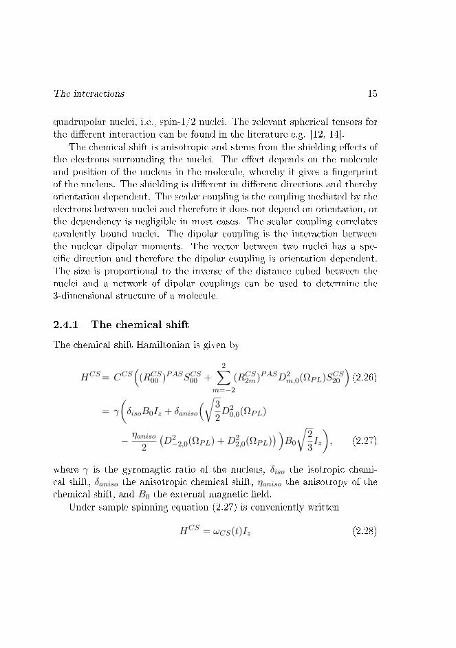
2.4.1 The chemical shift
The chemical shift Hamiltonian is given by
HCS= CCS(
(RCS00 )PASSCS00 +2∑
m=−2
(RCS2m)PASD2m,0(ΩPL)SCS20
)(2.26)
= γ
(δisoB0Iz + δaniso
(√3
2D2
0,0(ΩPL)
− ηaniso2
(D2−2,0(ΩPL) +D2
2,0(ΩPL)) )B0
√2
3Iz
), (2.27)
where γ is the gyromagtic ratio of the nucleus, δiso the isotropic chemi-cal shift, δaniso the anisotropic chemical shift, ηaniso the anisotropy of thechemical shift, and B0 the external magnetic eld.
Under sample spinning equation (2.27) is conveniently written
HCS = ωCS(t)Iz (2.28)

16 Magic-angle spinning solid-state NMR
using the denitions
ωCS(t) =2∑
m=−2
ωCSm eimωrt = ωiso +2∑
m=−2
ωanisom eimωrt, (2.29)
withωiso = γδisoB0
and
ωanisom = ωaniso
(D
(2)0,−m(ΩCS
PR)
− ηaniso√6
(D
(2)−2,−m(ΩCS
PR) +D(2)2,−m(ΩCS
PR)))
d(2)−m,0(βRL).
withωaniso = γδanisoB0.
Using AHT to rst order only m = 0 contributes and for MAS, i.e.,β = arccos
√1/3 ∼ 54.74 giving d(2)
0,0(βRL) = 0, only the isotropic shift isleft (higher-order AHT reveals spinning side bands) as seen in gure 1.1
H(1)CS = ωisoIz. (2.30)
2.4.2 The scalar coupling
The scalar coupling Hamiltonian is given by
HJ = CJ(RJ00)PASSJ00 = ωJ2I · S = ωJ2(IxSx + IySy + IzSz), (2.31)
where ωJ = 2πJ , J being the coupling constant and I and S the two couplednuclei. However, for weak coupling, i.e., ωJ signicantly smaller than theresonance frequency dierence of the two nuclei, the coupling Hamiltoniantruncates to
HJ = ωJ2IzSz. (2.32)

The interactions 17
2.4.3 The dipolar coupling
The dipolar coupling Hamiltonian is given by
HD = CD(RD20)PASD20,0(ΩPL)SD20 (2.33)
= −2γIγS~√
3
2
µ0
4πr−3ISD
20,0(ΩPL)
1√6
(3IzSz − I · S)
= −γIγS~µ0
4πr3IS
D20,0(ΩPL)(3IzSz − I · S) (2.34)
where γI and γS are the gyromagnetic ratios of nuclei I and S, respectively,~ is Planck's constant divided by 2π, and µ0 is the permittivity of vacuum.By denition of the dipolar coupling constant bIS = −γIγS~µ0/(4πr
3IS) this
is writtenHD = bISD
20,0(ΩPL)(3IzSz − I · S) (2.35)
Under sample spinning, equation (2.35) is conveniently written
HD = ωD(t)(3IzSz − I · S) (2.36)
using the denition
ωD(t) =2∑
m=−2
ωDmeimωrt (2.37)
withωDm = bISD
20,−m(ΩPR)d
(2)−m,0(βRL). (2.38)
Often this is further elaborated, giving D20,−m(ΩPR) explicitly since the
dipolar coupling tensor is rotation symmetric around the axis connectingthe two nuclei, i.e., αPR can arbitrarily be set to zero, yielding the simpleexpression
ωDm = bISd20,−m(βPR)eimγPRd
(2)−m,0(βRL). (2.39)
Under MAS the coecients
ωD0 = 0, ωD±1 = − bIS
2√
2sin 2βPRe
±iγPR , ωD±2 =bIS4
sin2 βPRe±2iγPR
(2.40)

18 Magic-angle spinning solid-state NMR
are obtained.Using AHT to rst order two useful results are obtained. In case of
heteronuclear dipolar coupling the large resonance frequency dierence be-tween the two nuclei truncates the dipolar coupling to the term commutingwith Iz and Sz, i.e.,
HD = ωD(t)2IzSz (2.41)
and secondly, under MAS, the dipolar coupling is averaged to zero to rstorder
H(1)D = 0, (2.42)
since terms with m 6= 0 are modulated by eimωrt and ωD0 = 0 under MAS.

Chapter 3
Resolution enhancement by
dipolar-driven spin-state
selection
The increased line width of carbonyl carbon due to the homonuclear scalarcoupling to the α-carbon remains problematic in the direct dimension. Thisis unfortunate since it can lead to overlapping / unresolved peaks and thereofambiguous resonance assignment in the dimension where resolution comesfor free with respect to experiment time. Four approaches to remove theline broadening due to the scalar coupling have been published: 1) selectivehomonuclear scalar decoupling during acquisition [21], 2) scalar coupling-based spin-state selective excitation protocols [2225], 3) post-acquisitionprocessing removal by J-deconvolution [26], and 4) optimal control (OC)based dipolar-driven spin-state selective coherence transfer [5].
The decoupling based method consists of interleaved acquisition andselective homonuclear decoupling pulses. This approach is technically chal-lenging and the S/N (signal-to-noise ratio) is decreased since the samplingperiod is diminish by the pulse lengths and ring-down periods. Furthermore,attention has to be paid to avoid recoupling conditions and Hartmann-Hahnmatching [27] (i.e., matching of the dierence between the two applied
19

20 Resolution enhancement by dipolar-driven spin-state selection
rf-eld strengths and 0,±1,±2 times the sample spinning frequency),whereof avoiding the last possibly leads to the requirement of undesirablehigh-power proton decoupling.
The scalar coupling-based spin-state selective excitation protocols havebeen implemented as IPAP (in-phase anti-phase) [22, 23], as an S3 (spin-state selective) version of the INADEQUATE (Incredible Natural Abun-dance Double Quantum Transfer Experiment) [28] experiment [24], and asa pure S3E (spin-state selective excitation) building block [25]. The IPAPprotocol uses selective π/2- and π-pulses on the carbonyl carbon and α-carbon (and for the double IPAP as well on the Cβ) to obtain in-phaseand anti-phase spectra which can be summed and subtracted to producesingle spin-state line shapes. The S3 methods likewise rely on selectivepulses for establishing single spin-state magnetisation before acquisition. Inthe INADEQUATE-S3 experiment, the second half of the normal INAD-EQUATE experiment is substituted for an S3 element which converts thedouble-quantum magnetisation to single spin-state magnetisation and thesingle spin-state line shapes are directly obtained [2932]. The S3E experi-ment consists of acquisition of two spectra which can be manipulated intosingle spin-state line shapes. All of these sequences makes use of the weakscalar coupling for spin-state manipulation and the pulse sequences are oflength 10 ms (25 ms for the double IPAP), 20 ms, and 5 ms, respectively,for IPAP, INADEQUATE-S3, and S3E. Due to relaxation, these long pulsesequences unavoidably lead to a lower S/N, however, of most importancethey all depend on very high-power proton decoupling (156 kHz TPPM,100 kHz XiX (x-inverse-x), and 85 and 150 kHz SPINAL64 (depending onthe system), respectively, according to the published experiments). Thismakes these sequences unattractive for temperature sensitive samples andsalty samples which are heated extensively by the electric eld of the irradi-ation. E-eld free [3336] probes constitute an alternative, however, theseprobes normally do not provide suciently strong rf-elds. The MAS ratesused were 635, 22.5, and 20 kHz for IPAP, INADEQUATE-S3, and S3E,respectively, and a comparison shows that the sequences fail to cover theregime of relatively slow MAS without very high-power decoupling.
The post-acquisition processing approach consists of maximum-entropy

Analytical dipolar-driven spin-state selection 21
reconstruction and deconvolution of the scalar coupling evolution (cosπJt).This approach can be applied in the direct as well as the indirect dimensionand implementation of new pulse sequences are avoided. In this way thepulse sequences are not enlarged leading to a better S/N. Drawbacks arethe risk of introduction of artefacts to the spectrum.
The OC-based dipolar-driven spin-state selective coherence transfer con-sists of an OC developed element which, by use of the dipolar coupling,transfers in-phase Cα-magnetisation to single spin-state coherence on thecarbonyl carbon for detection. As such, the element has a double eectwhich can be both a pro and a con. OC-based sequences eectively inducethe desired manipulation, however, the actual mechanism is unknown whichimpedes subsequent analytical modications. The OC-based dipolar-drivenspin-state selective coherence transfer sequence is developed for a 700 MHzspectrometer and will possibly suer from the larger CSAs on stronger mag-nets.
The great attention / interest in avoiding the line broadening due to thescalar coupling is enlightened by the growth in publications using the abovementioned techniques, e.g., [21] and [26] both having around 10 citations and[23] having nearly 50 citations according to SciFinder, Sept. 2012. More-over, improvements are continually being presented as e.g. the recently pub-lished incorporation of the INADEQUATE-S3 in a double-quantum / zero-quantum ultra-fast MAS (60 kHz) experiment [37] giving unprecedentedcombined resolution and sensitivity.
In this chapter the work for developing new protocols for analyticaland optimal control based dipolar-driven spin-state selection schemes arepresented.
3.1 Analytical dipolar-driven spin-state selection
This section describes the work done in order to obtain an analytically de-veloped dipolar-driven spin-state selection protocol. The protocol or pulsesequence makes use of the EXPORT (EXPonentially mOdulated RecouplingexperimenT) [38] magnetisation transfer element for homonuclear spins.

22 Resolution enhancement by dipolar-driven spin-state selection
This element is described in section 3.1.1. The combination of dierentEXPORT elements in a pulse sequence providing anti-phase magnetisationis described in section 3.1.2 in which the interplay between theory, simula-tions, and experimental verications are elaborated.
3.1.1 Exponentially modulated recoupling
The EXPORT experiment can be used to transfer transverse or longitudinalmagnetisation from one spin to another via the dipolar coupling dependingon the applied rf-eld. The longitudinal version creates an eective Hamil-tonian acting in the DQ-space whereas the transverse version works in atilted DQ-space (see g. 3.1 left and middle), however, since the spin-stateselection sequence uses the transverse version this is investigated here.
The rf-Hamiltonian reads (the Zeeman interaction frame, U = e−iωrfFz ,leaving the Hamiltonian of a constant rf-eld time-independent is implied)
Hrf = CFx +Be−iCtFxFyeiCtFx , (3.1)
where Fi =∑
n Ini, Ini being the Cartesian operator for spin I, and C andB are constants. By use of equation (2.7), it is found that Hrf is left zero bythe transforms U1U2 = e−iCtFxe−iBtFy , so the interaction frame is chosento be described by these transforms. The chemical shift Hamiltonian (2.28)will be transformed as follows (cx = cosx and sx = sinx are used)
˜HCS = U †2U†1H
CSU1U2 = ωCS(t)U †2U†1IzU1U2
= ωCS(t) (IzcCtcBt − IxcCtsBt + IysCt)
= ωCS(t)√
23B0
12
(Iz(c(C−B)t + c(C+B)t
)
− Ix(s(C−B)t + s(C+B)t
)+ Iy2sCt
).
First-order AHT with a characteristic time τc = 4π/ωr is used to eval-uate the signicance of B and C for B = ±1/2,±1 and C ∈ Z. Upon

Analytical dipolar-driven spin-state selection 23
insertion of the Fourier series for ωCS(t), this yields
˜H(1)CS =
ωr4π
∫ 4π/ωr
0dt
ωiso +
j∑
m=−jωanisom eimωrt
×(Iz(c(C−B)t + c(C+B)t
)− Ix
(s(C−B)t + s(C+B)t
)+ Iy2sCt
)
= 0 for |C +B| > 2ωr and |C −B| > 2ωr, (3.2)
since m ∈ −2, . . . , 2, neither the isotropic chemical shift nor the CSA willbe recoupled to rst order if the conditions are fullled.
The similar calculation for the dipolar coupling becomes
HD = U †1HDU1 = ωD(t)U †1(3IzSz − I · S)U1
= ωD(t)3(IzSz
(12 + 1
4
(e−i2Ct + ei2Ct
))
+ (IySz + IzSy)i4
(e−i2Ct − ei2Ct
)
+ IySy(
12 − 1
4
(e−i2Ct + ei2Ct
)− 1
3I · S)).
For C > 2ωr all the terms with C will average out in the nal step of AHT,and for convenience these are left out (indicated by the ′) at this point andthe second transform becomes
˜H ′
D= ωD(t)3U †2
(IzSz
12 + IySy
12 − 1
3I · S)U2
= ωD(t)38
(IzSz
(2 + e−i2Bt + ei2Bt
)− (IxSz + IzSx)
× i(2 + e−i2Bt − ei2Bt
)+ IxSx
(2− (e−i2Bt + ei2Bt)
)+ 4IySy
− 83I · S
).
For the dipolar coupling under MAS ωDm 6= 0 for m ∈ −2,−1, 1, 2and only terms demodulated with e±i2Bt, 2B = mωr will contribute in rst-order AHT (for convenience b = B/ωr which is assumed equal to 1/2 or 1,

24 Resolution enhancement by dipolar-driven spin-state selection
2Ix Sx-2IySy
2Ix Sy
+2IySx
Iz +Sz
2IzSz-2Ix Sx
2IzSx+2Ix Sz
Iy +Sy
Γ
dΘ
dt=ΚH ΒL
2IzSz -2Ix Sx 2IzSx +2Ix Sz
Iy +Sy
Figure 3.1: Double-quantum space (left), the tilted double-quantum space (mid-dle), and the EXPORT (y-to-y) magnetisation transfer visualised in the tilteddouble-quantum frame illustrating the γPR- and βPR-spreading: Dierences inthe γPR-angle resulting in dierent trajectories while dierences in the βPR-angleresult in dierent rotation rates, κ.
i.e. recoupling, is introduced):
˜H(1)D =
ωr2π
∫ 2π/ωr
0dt
j∑
m=−jωDme
imωrt 38
((IzSz − IxSx)
(e−i2Bt + ei2Bt
)
− (IxSz + IzSx) i(e−i2Bt − ei2Bt
)− 8
3I · S)
= 38
((IzSz − IxSx)
(ωD2b + ωD−2b
)
− (IxSz + IzSx) i(ωD2b − ωD−2b
) )
= κb((IzSz − IxSx)c2bγ + (IxSz + IzSx)s2bγ
)(3.3)
= κbe−i2bγSy(IzSz − IxSx)ei2bγSy , (3.4)
where the Euler angles here and in the following refer to the transform fromPAS to RS, i.e., ΩPR. κb is determined from ωDm equation (2.40) to
κ1/2 = − bIS
4√
2s2β and κ1 =
bIS8s2β (3.5)
with bIS (given section 2.4.3) being the dipolar coupling constant.The nal result (3.4) shows how the EXPORT rotates (and γ encodes)
magnetisation in the tilted double-quantum subspace shown in g. 3.1

Analytical dipolar-driven spin-state selection 25
(right). By changing the phase of the rf-Hamiltonian successively by π/2all four Hamiltonians are obtained
˜H(1)D =
κbe∓i2bγSy(IzSz − IxSx)e±i2bγSy 0, π
κbe±i2bγSy(IzSz − IySy)e∓i2bγSy π/2, 3π/2
(3.6)
for rf Hamiltonians
Hrf =
±CFx +Be∓iCtFxFye
±iCtFx 0, π±CFy ∓Be∓iCtFyFxe±iCtFy π/2, 3π/2.
(3.7)
The evolution of Iy-magnetisation (illustrated in g. 3.1 (right)) gov-erned by the EXPORT average Hamiltonian is calculated in the togglingframe of U = e−iγSy , i.e., rst the description is transferred to the framecharacterised by the transformation U = e−iγSy
U †IyU = Iy.
Secondly, the evolution due to the Hamiltonian κb(IzSz − IxSx) (3.4) isdetermined using [IzSz, IxSx] = 0
eiκbIxSxte−iκbIzSztIyeiκbIzSzte−iκbIxSxt
= eiκbIxSxt(Iycκbt/2 − 2IxSzsκbt/2
)e−iκbIxSxt
= Iyc2κbt/2
− (2IxSz + IzSx)cκbt/2sκbt/2 − s2κbt/2
Sy,
and nally the description is transferred back
U(Iyc
2κbt/2
− (2IxSz + IzSx)cκbt/2sκbt/2 − s2κbt/2
Sy
)U † =
Iyc2κbt/2
− ((2IxSz + IzSx)c2bγ + (2IxSx− IzSz)s2bγ)cκbt/2sκbt/2−Sys2κbt/2
.
For a powder, the γ angle takes values 0 to 2π and the result is averagedwhereby the nal result is obtained
IyHEXPORTt−−−−−−−→ Iyc
2κbt/2
− Sys2κbt/2
. (3.8)
The eect of the EXPORT elements on a coupled 2-spin system becomes atransfer of magnetisation from e.g. Iy to −Sy for κbt = π. The theoretical

26 Resolution enhancement by dipolar-driven spin-state selection
bIS
2 π
B=ωr/2B=ωr
t
Figure 3.2: Analytically determined transfer eciencies for the two EXPORTrecoupling conditions for a powder.
transfer eciency for the two recoupling conditions are shown in g. 3.2and the maximum transfer is 73.3 % due to the spread of βPR angles in apowder.
The implementation of the rf-elds on the spectrometer is obtained byevaluating the x-, y-, and z-component of the Hamiltonian (3.1) and calcu-lating the amplitude A and phase φ from the x- and y-component and thephase correction from the z-component:
Hrf = CFx +BcCtFy +BsCtFz
A =√C2 +B2c2
Ct φ = φxy −∫ t
0 BsCtdt = arctan BcCtC + B
C (cCt − 1).
The three other Hamiltonians are obtained by adding nπ/2 according toeqn. (3.6).
Characteristics of the EXPORT elements include broadbandedness [38],compensations for inhomogeneity in the applied rf-elds can be incorporatedby alternating the sign of C every 1/C period (in analogy with the schemepresented in [39]), and for large C-values no 1H-decoupling is required [38].
For completeness the average Hamiltonian for the scalar coupling duringthe EXPORT is determined. The scalar coupling is isotropic and trans-forms as a rank 0 tensor. The rst part means that it is unaected by theinteraction frame rotation transformations and the second leaves it time-

Analytical dipolar-driven spin-state selection 27
independent even under MAS, i.e.,
˜HJ = HJ = ωJ2I · S. (3.9)
The time-independence renders AHT unnecessary and the scalar couplingis unaected by the EXPORT element. As will be evident, this has to betaken into consideration.
3.1.2 Dipolar-driven spin-state-selection
The analytical approach to achieve dipolar-driven spin-state selection wasfrom the beginning to combine dipolar recoupling elements. The idea camefrom a consideration of the long pulse sequences needed for spin-state se-lection using the scalar coupling (vide supra) which is a manifestation ofthe weakness of this interaction. In contrast, the dipolar coupling is a muchstronger interaction (J(CO − Cα) ∼ 55 Hz compared to BIS/2π ∼ 2.1kHz [40], however, recoupling scales this by e.g. 1/4
√2 for EXPORT with
b = 1/2, equation (3.5)) which in turn means that it is capable of fastertransfers of magnetisation. A challenge, however, is the intrinsic orientationdependence of this coupling.
The most promising recoupling sequence for the purpose of spin-stateselection is the EXPORT element. The advantages of the EXPORT ele-ment is its broadbandedness and the lack of need for 1H-decoupling. Thebroadbandedness is necessary, because of the wide spread in chemical shiftof the carbonyl carbon and the Cα which constitute the scalar coupling spinpair of most interest. The possibility of avoiding strong 1H-decoupling isperhaps the most important advantage of dipolar-driven spin-state selectionsince many biological samples are too sensitive for the application of strongproton decoupling over longer periods.
The dipolar-driven spin-state selection pulse sequence proposed is shownin gure 3.3. It consists of three EXPORT elements with B = ωr/2, B = ωr,and B = ωr/2, respectively, of which the lengths are parameters for optimi-sation. The eect of the sequence is determined as follows. The calculationis restricted to optimised EXPORT element lengths meaning that all rota-tion transformations are considered π/2-rotations. The calculation is carried

28 Resolution enhancement by dipolar-driven spin-state selection
EXPORTB=ωr
EXPORTB=ωr/2
m( )
n( ) EXPORT
B=ωr/2
m( )
Figure 3.3: The dipolar-driven spin-state selection pulse sequence consisting ofthree consecutive EXPORT elements here shown with C = 10ωr. The achievedsignal is supposed to be anti-phase and can be combined with a normal in-phasesignal in the post-acquisition processing in order to obtain a spin-state selectivespectrum. m,n ∈ N.
out in the toggling frame of U = e−iγSy for B = ωr/2 and U = e−i2γSy forB = ωr and initial x-phase magnetisation is assumed. Transforming to therst toggling frame yields
U †IxU = eiγSyIxe−iγSy = Ix,
and the evolution during the rst element becomes
e−iπ(IzSz−IxSx)Ixeiπ(IzSz−IxSx) = 2IySz.
The density operator is transferred to the next toggling frame
eiγSy2IySze−iγSy = 2IySzcγ − 2IySxsγ ,
and the evolution is determined
eiπ(IzSz−IxSx)(2IySzcγ − 2IySxsγ)eiπ(IzSz−IxSx) = 2Ixcγ − 2Izsγ .
The density operator is transferred back to the rst toggling frame
e−iγSy(Ixcγ − Izsγ)eiγSy = Ixcγ − Izsγ ,
and the last evolution becomes
e−iπ(IzSz−IxSx)(Ixcγ − Izsγ)eiπ(IzSz−IxSx) = 2IySzcγ − 2IySxsγ .

Analytical dipolar-driven spin-state selection 29
a b
Figure 3.4: Analytically determined transfer eciency for the dipolar-driven spin-state selection sequence g. 3.3 as function of the length of the EXPORT elementsand the dipolar-coupling constant (a) and the eciency as function of the βPRpowder angle for optimised t1 and t2 (b).
Finally, the description is transferred to the original frame
e−iγSy(2IySzcγ − 2IySxsγ)e−iγSy
= 2IySzc2γ + (2IySx − 2IySx)cγsγ + 2IySzs
2γ = 2IySz,
and the γ-dependency is refocused.The dependence of the pulse lengths can, if the full calculation was
carried out, be found to (after γ-averaging):
Ixcκ1t2/2cκ1/2t1 + 2IySzs2κ1/2t1/2
sκ1t2/2, (3.10)
where t1 indicates the length of the EXPORT elements with B = ωr/2 andt2 the length of the element with B = ωr in the pulse sequence. The pow-der averaged transfer eciency is depicted in gure 3.4, and the maximumtransfer for a powder is found to 59.6 %. Figure 3.4 right illustrates theorigin of the losses, i.e., the βPR-dependency of the transfer eciency underoptimised conditions. The low transfer eciency for βPR ∼ π/2 which hasa high weight in the averaging, unavoidably lowers the transfer eciency.
30 Resolution enhancement by dipolar-driven spin-state selection
Compared to the potential 100 % transfer for scalar coupling based exper-iments the calculated transfer eciency is relatively low, however, thesenumbers do not include relaxation which can be prominent especially forthe long pulse sequences based on scalar coupling transfers. Moreover, thedipolar-driven scheme will be applicable on sensitive samples for which thescalar coupling-based methods does not apply due to the required strongproton decoupling.
Returning to the eect of the scalar coupling on the proposed pulsesequence, the evolution during an EXPORT element of length t includingthe scalar coupling (3.9) was determined assuming initial Iy-magnetisation.The result is
12(Iy(c2ωJ t + c2κbt) + Sy(−c2ωJ t + c2κbt) + 2(IzSx − IxSz)s2ωJ t), (3.11)
with ωJ = 2πJ , J being the scalar coupling constant introduced section2.4.2. Even though the scalar coupling is weak compared to the dipolar cou-pling this will clearly aect the result. However, if the initial magnetisationis distributed equally on both nuclei in the spin pair, the eect disappears.If initial magnetisation α1Iy + α2Sy is assumed the result becomes
(α1 + α2)cκbt(Iy + Sy)
+ 12((α1 − α2)c2ωJ t(Iy − Sy) + 2(α1 − α2)s2ωJ t(IzSx − IxSz)),
which for α1 = α2 = α equals
αcκbt(Iy + Sy) = (c2κbt− s2
κbt)(Iy + Sy), (3.12)
and the result is identical to the result obtained without taking the scalarcoupling into account. Experimentally, it can be dicult to full this re-quirement, however, there will in most cases be magnetisation on both nucleidiminishing the eect of the scalar coupling.
In order to investigate in more detail the eciency of the spin-state selec-tion sequence, simulations using the SIMPSON simulation software [4143]on a typical CO-Cα spin system were conducted. The spin system is based

Analytical dipolar-driven spin-state selection 31
δiso/ppm δaniso/ppm ηanisoCO 170 -76 0.90Cα 50 -20 0.43
bIS/2π/kHz JIS/HzCO-Cα -2.142 55
Table 3.1: Spin system parameters for the CO-Cα 2-spin system used for simula-tions of the eciency of the spin-state selection sequence.
on the typical values given in [40]. Table 3.1 summarises the parametersand App. A.4 further elaborates on the spin system details.
The transfer eciency as function of the lengths of the EXPORT ele-ments, or actually the number of repetitions of the EXPORT element, i.e.,m and n in gure 3.3, was determined for 10 kHz MAS, C = 10ωr, rf-frequency corresponding to 110 ppm (i.e., halfway between the CO and theCα resonances), a digitisation of the waves of 250 steps per rotor periodcorresponding to steps of 400 ns, and a spectrometer frequency of 400 MHz(1H). The initial magnetisation is assumed Ix+Sx (I and S representing CO
and Cα, respectively). The powder averaging used the REPULSION scheme[44] with 66 α, β-angles and 10 γ-angles which prove sucient. The anti-phase intensity for CO and Cα as function of the lengths of the EXPORTelements is shown in gure 3.5 and the maximum transfer is determined to57.2 % to CO and to 58.4 % to Cα with m=10 and n=16 in both cases. In-clusion of 5 % rf-eld inhomogeneity reduces the transfer eciency to 35.4% and 37.3 %, respectively, with m=10 and n=12. The surprising reductionin eciency is found to originate mainly from the B = ωr recoupling con-dition being severely aected by rf-inhomogeneity even when incorporatedwith alternating sign on C (see p. 26) as is the case. This is also reected inthe shortened optimum length for the B = ωr recoupling condition (n=12instead of 16), while the length of the B = ωr/2 recoupling condition is pre-served. Sign-alternation of B in dierent schemes [39] has been examined,however, without success.
The experimental implementation was unsuccessful for larger amino

32 Resolution enhancement by dipolar-driven spin-state selection
0 0.5 1 1.5 2 01
23
4
-0.10
0.10.20.30.40.50.6
Norm
alis
ed tra
nsfe
r
Inphase to antiphase CO
t1 / ms
t2 / ms
Norm
alis
ed tra
nsfe
r
0 0.5 1 1.5 2 2.5 3 3.5 4
t2 / ms
0
0.5
1
1.5
2
t 1/ m
s
0 0.5 1 1.5 2 2.5 3 3.5 4
t2 / ms
0
0.5
1
1.5
2
t 1/ m
s
0
0.1
0.2
0.3
0.4
0.5
0 0.5 1 1.5 2 01
23
4
-0.10
0.10.20.30.40.50.6
Norm
alis
ed tra
nsfe
r
Inphase to antiphase Cα
t1 / ms
t2 / ms
Norm
alis
ed tra
nsfe
r
Figure 3.5: Transfer eciencies for the carbonyl (left) and the Cα (right) as func-tion of the lengths of the EXPORT elements in the spin-state selection sequencedetermined from simulations on a typical CO and Cα 2-spin system.
acids, however, on a uniformly 13C,15N-labelled glycine (99 % labelling)(Isotec, Sigma-Aldrich) sample, experimental conditions was establishedproving the ability of the spin-state selection pulse sequence to produceanti-phase magnetisation which, upon addition to the normal in-phase spec-trum, produced a spin-state selective spectrum with a highly reduced linewidth of the carbonyl resonance, gure 3.6. The experiment was conductedat a 400 MHz Bruker Avance II spectrometer (Bruker Biospin, Rheinstet-ten, Germany) equipped with a triple-resonance 2.5 mm probe. The pulsesequence consisted of a ramped CP (Cross Polarisation) [45, 46] for mag-netisation transfer from protons to x-phase carbon magnetisation followedby the spin-state selection sequence with the EXPORT elements incorpo-rated as wave les with C = ±10ωr (i.e. alternating the sign of C every1/C in order to make it robust towards rf-eld inhomogeneity) and 400ns step size. No proton decoupling was applied during the pulse sequenceexcept SPINAL64 [47] during acquisition. During the optimisation of the

Analytical dipolar-driven spin-state selection 33
170175
Reference
170175
δ (13C) / ppm
170175
FWHM=106.1 Hz FWHM=32.5 Hz
ns = 4 ns = 24ns = 20
t1=1.1 mst2=0.7 ms
Sum
Figure 3.6: Experimental solid-state spectra showing the carbonyl resonance of13C,15N-labelled glycine: Normal in-phase CP/MAS spectrum (left), anti-phasespectrum acquired by addition of the spin-state selection sequence to the pulsesequence used for the normal CP/MAS spectrum (middle), and the sum of thetwo spectra giving the S3E-spectrum with the improved line width (right). BothEXPORT rf-eld strength and EXPORT element lengths were optimised exper-imentally obtaining t1 = 1.1 ms and t2 = 0.7 ms. 400 MHz (1H) spectrometerfrequency, 135 kHz decoupling during acquisition, 1.5 ms CP of 30 kHz 13C and53 kHz 1H, 4 scans, 50 ms acquisition, no apodisation.
EXPORT element lengths, an x-phase spin-lock pulse was applied to thecarbon channel between the CP and the spin-state selection sequence inorder to guarantee x-phase magnetisation at the start of the sequence sincethe optimisation process was hindered by obscure line shapes. However,after optimum conditions with respect to EXPORT element lengths and rf-eld strength, the spin-lock was removed without observable changes to theline shapes. The optimisation solely focussed on the carbonyl resonance,however, signs of anti-phase line shapes was observed for the Cα resonanceas well.

34 Resolution enhancement by dipolar-driven spin-state selection
The obtained spin-state selective spectrum shows a line width reducedby impressively 145 % from 106 Hz to 32.5 Hz, however, on the expenseof signal intensity: in order to achieve the anti-phase spectrum, 6 timesas many scans are needed, i.e., a transfer eciency of 17 % correspond-ing to 28 % of the theoretical maximum and 52 % the maximum found insimulations including 5 % inhomogeneity. The optimum EXPORT elementlengths determined are shorter than those determined analytically as wellas by simulations, however, mainly the B = ωr element is shortened. Thediscrepancies are ascribed to relaxation which is not included in the sim-ulations, and to the rf-inhomogeneity sensitivity of the B = ωr recouplingcondition. The short experimentally determined optimum EXPORT ele-ment lengths and the low transfer eciency both stress the need for shortsequences and fast transfers in order to minimize relaxation losses.
δiso/ppm δaniso/ppm ηanisoCO 174 -76 0.90Cα 53 -20 0.43Cβ 40 -20 0.43Cγ 25 -20 0.43
bIS/2π/kHz JIS/HzCO-Cα -2145.1 55Cα-Cβ -2016.7 35Cβ-Cγ -1958.8 35CO-Cβ -515.11 0CO-Cγ -127.26 0Cα-Cγ -405.7 0
Table 3.2: Spin system parameters for the leucine CO-Cα-Cβ(-Cγ) 3- / 4-spinsystem used for simulations of the eciency of the spin-state selection sequencefor larger spin systems. The 3-spin system is obtained by removal of Cγ .
Having obtained experimental proof-of-concept on a glycine sample sim-ulations of longer spin-chains were conducted which fully explain the exper-imentally observed lack of performance on larger amino acids. Figures 3.7and 3.8 top row shows the transfer eciencies for the spin-state selection

Analytical dipolar-driven spin-state selection 35
0 0.2 0.4 0.6 0.8 1 0
1
2
-0.10
0.10.20.30.40.5
Norm
alis
ed tra
nsf
er
Inphase to antiphase CO
00.10.2
t1 / ms
t2 / ms 0 0.2 0.4 0.6 0.8 1 0
1
2
-0.10
0.10.20.30.40.5
Inphase to antiphase Cα
0 0.2 0.4 0.6 0.8 1 0
1
2
-0.10
0.10.20.30.40.5
Norm
alis
ed tra
nsf
er
00.10.20.3
t1 / ms
t2 / ms 0 0.2 0.4 0.6 0.8 1 0
1
2
-0.10
0.10.20.30.40.5
00.10.20.3
t1 / ms
t2 / ms
a
b
00.1
t1 / ms
t2 / ms
Figure 3.7: Transfer eciencies for the two spin-state selection sequences gure3.3 (top row) and 3.9 (bottom row) for the carbonyl (left column) and the Cα(right column) as function of the lengths of the EXPORT elements in the spin-state selection sequence determined from simulations on a 3-spin system resemblingCO-Cα-Cβ of leucine.
sequence for a 3-spin and a 4-spin system resembling CO-Cα-Cβ and CO-Cα-Cβ-Cγ of leucine, respectively. The spin systems were constructed usingSIMMOL [40] applying the geometry of residue 15 in Ubiquitin, pdb 1D3Z[48]. The parameters are summarised in Table 3.2 and further details aregiven in App. A.4. The optimum is seen to vanish for both the 3- (gure3.7 top row) and the 4-spin (gure 3.8 top row) system and the sequencebecomes unusable.
Since the dipolar coupling between the Cα and the Cβ is by far thestrongest dipolar coupling between CO-Cα and the rest of the spin system,it was assumed that this coupling was the main reason for the lack of per-

36 Resolution enhancement by dipolar-driven spin-state selection
a
b
0 0.2 0.4 0.6 0.8 1 0
1
2
-0.10
0.10.20.30.40.5
Norm
alis
ed tra
nsf
er
Inphase to antiphase CO
00.1
t1 / ms
t2 / ms 0 0.2 0.4 0.6 0.8 1 0
1
2
-0.10
0.10.20.30.40.5
Inphase to antiphase Cα
00.1
t1 / ms
t2 / ms
0 0.2 0.4 0.6 0.8 1 0
1
2
-0.10
0.10.20.30.40.5
Norm
alis
ed tra
nsf
er
00.10.20.3
t1 / ms
t2 / ms 0 0.2 0.4 0.6 0.8 1 0
1
2
-0.10
0.10.20.30.4
00.10.20.3
t1 / ms
t2 / ms
Figure 3.8: Transfer eciencies for the two spin-state selection sequences gure3.3 (top row) and 3.9 (bottom row) for the carbonyl (left column) and the Cα(right column) as function of the lengths of the EXPORT elements in the spin-state selection sequence determined from simulations on a 4-spin system resemblingCO-Cα-Cβ-Cγ of leucine.
formance, and the idea to refocus the unwanted part (i.e., the couplingsinvolving Cβ) of the recoupled (EXPORT) Hamiltonian was established.The concept, still being in its developmental process, was tested in simula-tions by introduction of selective π-pulses applied to the Cβ , as shown ingure 3.9. The refocussing pulses perturb the EXPORT average Hamilto-nians including the Cβ as follows, S representing Cβ and I representing acoupling partner e.g. Cα. The EXPORT Hamiltonian is (equation (3.4))
H = κb ((IzSz − IxSx)c2bγ + (IxSz + IzSx)s2bγ) .
For evaluation, the part following the Cβ refocusing pulse, is transferred to

Analytical dipolar-driven spin-state selection 37
EXPORTB=ωr
EXPORTB=ωr/2
m2
( ) ( )EXPORTB=ωr/2( )
πy,Cβ
m2
n2
πy,Cβ
EXPORTB=ωr( )
n2
EXPORTB=ωr/2
m2
( ) EXPORTB=ωr/2( )
πy,Cβ
m2
Figure 3.9: The dipolar-driven spin-state selection pulse sequence including theselective Cβ refocusing pulses. EXPORT elements are shown with C = 10ωr.
a toggling frame of U = e−iπSy , i.e.,
H2 = e−iπSyHeiπSy
= κb ((−IzSz + IxSx)c2bγ + (−IxSz − IzSx)s2bγ) .
By the use of additivity of average Hamiltonians equation (2.12) the averageHamiltonian over the entire element becomes
H1+2 = H +H2 = 0 (3.13)
for all dipolar couplings to Cβ . However, leaving all other interactionsunperturbed.
The eect of the refocusing pulses is enlightened by simulations, usingotherwise identical conditions, of the new pulse sequence and the result isshown in gures 3.7 and 3.8 (bottom row) for the 3- and 4-spin system,respectively. The success of removing the couplings to Cβ is evident andthe transfer eciencies of 38.3 % (CO, 3-spin), 38.5 % (Cα, 3-spin), 37.1 %(CO, 4-spin), and 35.7 % (Cα, 4-spin) all for m=10, n=14 are comparableto the 2-spin transfer eciencies.
The experimental implementation of the improved spin-state selectionsequence, however, represents a challenge. The experimental incorporationof selective pulses is traditionally done by longer low rf-eld strength Gaus-sian pulses. On the otherwise unaected spin, these pulses induce unwantedchemical shifts which has to be compensated. Furthermore, rotor synchro-nisation has to be assured. Secondly, the chemical shift of the Cβ varieswith amino acid from 30 70 ppm [49] which hinders a general approach.

38 Resolution enhancement by dipolar-driven spin-state selection
A more general approach would be to make a CO-selective pulse com-bined with a hard refocusing pulse and a half-rotor period delay. Thisrenders only couplings to the carbonyl carbon active. The approach is re-ferred to as RADAR (Rotor Assisted DipolAr Refocusing) [50] and uses theγ-dependency of the Hamiltonian, i.e., a delay of half a rotor period has thesame eect as an addition of π to the γ-angle which in turn changes the signof both cosine and sine in the Hamiltonian (3.4); the double sign changerenders only the carbonyl couplings active. However, the implementation isstill challenging because of the chemical shifts induced during the selectivepulses. The implementation is subject to future developmental work.
3.2 Numerical dipolar-driven spin-state selection
In this section the developmental work on numerically optimisation of spin-state selection sequences is described. The numerical approach makes useof the optimal control (OC) procedure build in to SIMPSON [4143, 51].
Firstly, the OC procedure is described briey and secondly the resultsregarding the spin-state selection are presented.
3.2.1 Optimal Control
Optimal control (OC), as applied to NMR pulse sequence development [51],is a numerical procedure which optimises the RF-eld for a given purposee.g. for maximal transfer of magnetisation from one state to another stateor to create a desired Hamiltonian which are the two options included in theSIMPSON [4143] simulation software. Many boundary conditions can beincluded in the optimisation procedure as for instance the maximum timefor the given transfer or limitations on the outcome of magnetisation trans-fer to undesired states. A drawback of OC is that the produced sequenceis specic to the given spin-system and seldom interpretable, however, ex-amples of OC-inspired analytically developed sequences are seen, e.g [52].Moreover, with the optimisation procedure incorporated in SIMPSON, i.e.,the GRAPE (GRadient Ascent Pulse Engineering) [51] algorithm only alocal optimum is found (which could or could not be identical to the global

Numerical dipolar-driven spin-state selection 39
optimum) and many parallel optimisations are needed with random initialpulse sequences in order to (at least) have a good chance of nding anoptimum which provides an ecient pulse sequence.
The optimisation procedure is briey summarised in the following [43,51].
The Hamiltonian consists of the internal Hamiltonian (chemical shifts,dipolar couplings and scalar couplings) and the Hamiltonian of the rf-irradiation given by
Hrf (t) =∑
i
(ωixrf (t)Iix + ωiyrf (t)Iiy
), (3.14)
where the sum is over the nuclei in the spin system. ωixrf (t) and ωiyrf (t), rep-resenting the rf-amplitudes of x- and y-phase, are discretised and constitutethe parameters for optimisation.
For the optimisation of transfer from an initial state ρ(0) to a naldesired state ρd(tN ) the forward and backward propagated density operatorsare calculated (given initial discretised ωixrf (t) and ωiyrf (t), i.e., ωixn and ωiynfor n ∈ 1, . . . , N and Un(tn+1, tn) = e−iH(tn)(tn+1−tn))
ρ(tn) = Un(tn, tn−1) . . . U1(t1, t0)ρ(0)U †1(t1, t0) . . . U †n(tn, tn−1) (3.15)
ρd(tn) = U †n+1(tn+1, tn) . . . U †N (tN , tN−1)ρd(tN )
×UN (tN , tN−1) . . . Un+1(tn+1, tn), (3.16)
and compared in terms of the norm squared inner product
|〈ρd(tn)|ρ(tn)〉|2 =∣∣∣Tr
ρd(tn)†ρ(tn)
∣∣∣2
(3.17)
for each digitisation step. A gradient is determined based on the dierence(and possibly other constraints) and ωixn and ωiyn for each step are updatedaccordingly. The process is then repeated.
3.2.2 Optimal control based spin-state selection
By use of optimal control, design of spin-state selective sequences for bio-logical solid-state NMR is the goal. The optimal control based development

40 Resolution enhancement by dipolar-driven spin-state selection
facilitates the use of the strong dipolar couplings among neighbouring car-bon nuclei to achieve spin-state selective coherences, however, the optimi-sation procedure could result in a sequence using both scalar and dipolarcouplings in order to achieve the desired manipulation.
A sequence, which produces the desired spin-state e.g. 2IxSα is de-termined by stating desired and undesired magnetisation pass-ways. Thisconstitutes the target function which is maximised by the optimisation pro-cedure. The gradient of the target function with respect to amplitude andphase of each pulse segment is calculated and used iteratively to accomplishthe optimisation. To achieve a broadbanded sequence, the optimisation isperformed over a range of isotropic chemical shifts representing the CO-Cα-spin system. In the case of a successful optimisation, a wave (amplitudeand phase) which induces the desired magnetisation transfer, is generated.
The OC procudure, in which desired and undesired initial and targetstates are provided for the optimisation procedure, was chosen for the devel-opment of spin-state selection sequences. Dierent combinations of desiredand undesired states were tried, however, the most successful stayed similarto the combination in Ref. [5] with the slight change that the initial andnal states were adjusted to the same spin e.g. S3E (spin-state selective ex-citation) as opposed to S3CT (spin-state selective coherence transfer). Thisis summarised in the following desired transfers
IxSα −→ IxSα (3.18)
IxSβ −→ IxSα (3.19)
combined with the unwanted transfers
IxSα −→ IxSβ (3.20)
IxSβ −→ IxSβ. (3.21)
Optimisation for anti-phase magnetisation (which could in turn be combinedwith in-phase magnetisation in order to yield a spin-state selective spec-trum) and other ways of expressing the spin-state selection (e.g. Ix −→ IxSαcombined with the unwanted Ix −→ IxSβ) was also tried, however, less suc-cessfully.
Numerical dipolar-driven spin-state selection 41
Pre-testing of optimisation constraints
A pulse duration of 2 ms was found to provide the best success rate mea-sured on the fraction of waves producing a reasonable transfer. That is,normally e.g. ve to ten optimisations with random initial waveforms wereexecuted in parallel and the 2 ms pulse duration returned more reasonabletransfers compared to 1 ms, 3 ms, and 5 ms pulse durations. Moreover, amaximum rf-eld strength of 25 kHz (25, 50, and 100 kHz limits were tried)did likewise provide most waves providing reasonable transfers. A step size(the digitisation of the wave) of 1 µs was used to ensure compatibility withthe spectrometer. Potentially 400 ns steps could be implemented on theBruker Avance II and III spectrometers, however, a ner digitisation willresult in longer computation times for the optimisations. Finally, a seven byseven grid of the chemical shifts for the CO and Cα resonances was appliedin order to ensure broadbandedness of the generated waveforms. Initially, afour by seven (CO by Cα chemical shift) grid was used which, however, oftenresulted in wavy patterns in the resulting transfer eciency as function ofthe CO and Cα chemical shifts. This error was nearly eliminated by use ofthe seven by seven grids.
Optimisation conditions
In addition to the parameters mentioned in the foregoing section spin sys-tem, spectrometer and MAS frequency, powder averaging and optimisationparameters have to be dened. The spin system parameters used wereidentical to table 3.1, however, with diering Euler angles for the dipolarcoupling according to [5] as described in App. A.4. The isotropic chemicalshifts were varied in the array given by a CO chemical shift of 163.1, 165.4,167.7, 170, 172.3, 174.6, 176.9 ppm and a Cα chemical shift of 37.6, 41.8,46, 50.2, 54.4, 58.6, 62.8 ppm and an oset of 105.9 ppm was used (halfwaybetween CO and Cα ). The MAS frequency was set to 10.7 kHz in orderto avoid rotational resonance between carbonyl and aliphatic resonances atthe spectrometer frequency of 500 MHz (1H). The powder averaging usedthe REPULSION scheme [44] with 20 α, β-angles and 10 γ-angles.

42 Resolution enhancement by dipolar-driven spin-state selection
Experimental verication
The experimental testing of the generated waves were conducted at a BrukerAvance III 500 MHz (1H) spectrometer (Bruker Biospin, Rheinstetten, Ger-many) equipped with a triple-resonance 4 mm probe. The MAS was ad-justed to 10.7 kHz and the amplitude of the waves (incorporated as waveles) was optimised for each wave.
The pulse sequence consisted of a ramped CP (Cross Polarisation) [45,46] for magnetisation transfer from protons to x-phase carbon magnetisationfollowed by the OC developed wave with a 1 µs step size. CW decouplingwas applied to the protons simultaneous to the wave and SPINAL64 [47]decoupling was applied during acquisition.
Several samples were used for testing (e.g. uniformly 13C,15N-labelledalanine, threonine and a sample of brils of the peptide SSNFGAILSS la-belled on FGAIL), however, the initial tests used uniformly 13C,15N-labelledglycine (99 % labelling) (Isotec, Sigma-Aldrich).
Results and discussion
The rst series of successful optimisations using the parameters stated inthe previous subsections resulted in a couple of waves (i.e. series of am-plitude and phase) generating a broadbanded transfer of in-phase carbonylmagnetisation (in the following Ix) to spin-state selective carbonyl magneti-sation (IxSα, S representing Cα) measured on the 2-spin CO-Cα system alsoused for the optimisation procedure. These sequences were tested experi-mentally on uniformly 13C,15N-labelled glycine, whereby the most ecientwave was identied. This wave is depicted in gure 3.10 (tabulated valuesin App. C) and the broadbandedness is evidenced by simulations of trans-fer and suppression eciencies as function of varying CO and Cα chemicalshifts in gure 3.11. The experimental spectrum is shown gure 3.12.
Firstly, the simulation results show a wave capable of generating thedesired transfer of magnetisation. The wave itself is not interpretable, thatsaid, no advanced analyses have been undertaken in order to gain an under-standing of the wave. Secondly, the eciency is considered. Nearly exactly

Numerical dipolar-driven spin-state selection 43
0
2
4
6
8
ωrf/2π
/ kH
z
-100
0
100
0 0.2 0.4 0.6 0.8 1 1.2 1.4 1.6 1.8 2
Phase
/ (°)
Excitation time / ms
Figure 3.10: The phase (top) and amplitude (bottom) of the 13C rf-led of themost ecient S3E wave determined from the set of OC optimised waves on theCO-Cα spin system.
0.5 IxSα is generated (gure 3.11) which considering that
Ix = Ix(Sα + Sβ) (3.22)
corresponds to that the IxSα intensity is kept while the IxSβ intensity issuppressed. It could be hypothesised that intensity could be transferredfrom IxSβ to IxSα, while keeping the original IxSα intensity resulting inan IxSα intensity over 0.5. This is, however, according to the optimisationresult not possible and theoretical bounds [53, 54] give the same answer.
The theoretical maximum emax and minimum emin transfers from oneoperator A to another operator B in Liouville space is given by
emax =a · b
TrA†A (3.23)
emin =a · b′
TrA†A , (3.24)
where a and b are the vectors of the eigenvalues of A and B ordered withrespect to magnitude and b′ representing the reverse ordering.

44 Resolution enhancement by dipolar-driven spin-state selection
160 165 170 175 180 185 190 3040
5060
7080
-0.3-0.2-0.1
00.10.20.30.40.5
Norm
alis
ed in
tensi
ty
Ix to IxSα
-0.2-0.1
00.10.20.30.4
δ(CO) / ppm
δ(Cα) / ppm
Norm
alis
ed in
tensi
ty
160 165 170 175 180 185 190 3040
5060
7080
-0.3-0.2-0.1
00.10.20.3
Norm
alis
ed in
tensi
ty
Ix to IxSβ
-0.2-0.1
00.10.2
δ(CO) / ppm
δ(Cα) / ppm
Norm
alis
ed in
tensi
ty
Figure 3.11: Transfer (left) and suppression (right) eciency as function of theCO and Cα chemical shift for the wave gure 3.10 determined from simulations onthe CO-Cα spin system identical to the spin system used during the optimisation.
Applied to the given transfer, the maximum is determined to be 0.5:
Ix =1
2
(0 11 0
)⊗(
1 00 1
)=
0 0 1/2 00 0 0 1/2
1/2 0 0 00 1/2 0 0
(3.25)
IxSα =1
2
(0 11 0
)⊗(
1 00 0
)=
0 0 1 00 0 0 01 0 0 00 0 0 0
. (3.26)
The eigenvalue vectors are obtained by diagonalisation to
vIx =
−1/2−1/21/21/2
and vIxSα =
−1/200
1/2
. (3.27)
Finally, the result is obtained
emax(Ix → IxSα) =1
2. (3.28)

Numerical dipolar-driven spin-state selection 45
Figure 3.12: Experimental CP/MAS 13C-spectra of reference (black) and OC de-veloped S3E sequence (wave gure 3.10) on uniformly 13C labelled glycine powdershowing the carbonyl resonance. 10.7 kHz MAS, 500 MHz (1H) spectrometer fre-quency, 100 kHz decoupling, 1.4 ms CP of 35 kHz 13C and 46 kHz 1H, 4 scans, 35ms acquisition, no apodisation. Amplitude of the wave was optimised for optimumspin-state selection on the carbonyl.
On this basis, it can be concluded that the 0.5 intensity is most satisfac-tory. The suppression limit of IxSβ can be checked using equation (3.24):
IxSβ =1
2
(0 11 0
)⊗(
0 00 1
)=
0 0 0 00 0 0 10 0 0 00 1 0 0
⇒ v′IxSβ = v′IxSα ⇒ emin(Ix → IxSα) = −1
2. (3.29)
With the minimum IxSβ intensity being negative, optimum suppressioncorresponds to an intensity of zero which indeed is theoretically possible.
Having obtained the theoretical bounds, the eciency of the wave is sat-isfactory according to the simulation. Only tiny increases of IxSα intensityare theoretically possible, however, the suppression of IxSβ intensity couldbecome a little better.
Proceeding to the experimental results gure 3.12, the eciency is lesssatisfactory. The suppression of IxSβ intensity is fair, however, the IxSα

46 Resolution enhancement by dipolar-driven spin-state selection
160 165 170 175 180 185 190 3040
5060
7080
-0.3-0.2-0.1
00.10.20.3
No
rma
lise
d in
ten
sity
Ix + Sx to IxSβ
-0.2-0.1
00.10.2
δ(CO) / ppm
δ(Cα) / ppm
No
rma
lise
d in
ten
sity
160 165 170 175 180 185 190 3040
5060
7080
-0.3-0.2-0.1
00.10.20.30.40.50.6
No
rma
lise
d in
ten
sity
Ix + Sx to IxSα
-0.2-0.1
00.10.20.30.40.5
δ(CO) / ppm
δ(Cα) / ppm
No
rma
lise
d in
ten
sity
Figure 3.13: Initial magnetisation on both spins: Transfer (left) and suppression(right) eciency for initial x-phase magnetisation on both nuclei as function of theCO and Cα chemical shift for the wave gure 3.10 determined from simulations onthe CO-Cα spin system identical to the spin system used during the optimisation.
160 165 170 175 180 185 190 3040
5060
7080
-0.2
-0.1
0
0.1
0.2
0.3
No
rma
lise
d in
ten
sity
Ix to IxSβ
-0.10
0.10.2
δ(CO) / ppm
δ(Cα) / ppm
No
rma
lise
d in
ten
sity
160 165 170 175 180 185 190 3040
5060
7080
-0.3-0.2-0.1
00.10.20.30.40.5
No
rma
lise
d in
ten
sity
Ix to IxSα
-0.2-0.1
00.10.20.30.4
δ(CO) / ppm
δ(Cα) / ppm
No
rma
lise
d in
ten
sity
Figure 3.14: Rf-inhomogeneity: Transfer (left) and suppression (right) eciencyincluding 5 % rf-inhomogeneity as function of the CO and Cα chemical shift for thewave gure 3.10 determined from simulations on the CO-Cα spin system identicalto the spin system used during the optimisation.

Numerical dipolar-driven spin-state selection 47
160 165 170 175 180 185 190 3040
5060
7080
-0.2-0.1
00.10.20.30.4
No
rma
lise
d in
ten
sity
Ix to IxSα
-0.10
0.10.20.3
δ(CO) / ppm
δ(Cα) / ppm
No
rma
lise
d in
ten
sity
160 165 170 175 180 185 190 3040
5060
7080
-0.3-0.2-0.1
00.10.20.30.40.5
No
rma
lise
d in
ten
sity
Ix to IxSβ
-0.2-0.1
00.10.20.30.4
δ(CO) / ppm
δ(Cα) / ppmN
orm
alis
ed
inte
nsi
ty
160 165 170 175 180 185 190 3040
5060
7080
-0.3-0.2-0.1
00.10.20.30.40.5
No
rma
lise
d in
ten
sity
Ix to IxSβ
-0.2-0.1
00.10.20.30.4
δ(CO) / ppm
δ(Cα) / ppm
No
rma
lise
d in
ten
sity
160 165 170 175 180 185 190 3040
5060
7080
-0.2-0.1
00.10.20.30.4
No
rma
lise
d in
ten
sity
Ix to IxSα
-0.10
0.10.20.3
δ(CO) / ppm
δ(Cα) / ppm
No
rma
lise
d in
ten
sity
160 165 170 175 180 185 190 3040
5060
7080
-0.3-0.2-0.1
00.10.20.30.40.5
Norm
alis
ed in
tensi
ty
Ix to IxSβ
-0.2-0.1
00.10.20.30.4
δ(CO) / ppm
δ(Cα) / ppm
Norm
alis
ed in
tensi
ty
160 165 170 175 180 185 190 3040
5060
7080
-0.2-0.1
00.10.20.30.4
Norm
alis
ed in
tensi
ty
Ix to IxSα
-0.10
0.10.20.3
δ(CO) / ppm
δ(Cα) / ppm
Norm
alis
ed in
tensi
ty
Figure 3.15: Spin system dependency: IxSα (left) and IxSβ (right) intensity asfunction of the CO and Cα chemical shift for the wave gure 3.10 determined fromsimulations. Shown are simulations for a 2-spin system using the typical valuesgiven in [40] (top) and a 2- and 3-spin system resembling CO-Cα(-Cβ) of leucine(residue 15 in Ubiquitin pdb 1D3Z [48]).

48 Resolution enhancement by dipolar-driven spin-state selection
intensity corresponds to only 60 % of the expected. Meanwhile, relaxationis not included in the theoretical bounds nor in the simulations, and un-avoidably leads to decreased experimental eciency. The wave was furthertested on larger molecules such as alanine and the peptide FGAIL, whereno reasonable results could be obtained (not shown). This was indeed sur-prising and let to a consideration of the eect of 1) initial magnetisation onboth spins, 2) rf-inhomogeneity and 3) spin system geometry and size.
Figure 3.13 shows the result of a simulation with initial x-phase mag-netisation on both CO and Cα. The eect is not dramatic, only tiny in-creases in the desired spin state intensity is found. This is possible sinceemax(Ix+Sx → IxSα) = 1. With the higher bound, it is tempting to initiatean optimisation of this process, however, this will result in a combined S3Eand S3CT sequence.
Figure 3.14 shows the eect of including an rf-inhomogeneity of 5 %.The eect is far too small to explain the lack of experimental performance.
Finally, simulations using a 2-spin system with Euler angles correspond-ing to the angles indicated for a CO-Cα spin pair in [40] (gure 3.15 top)and a 2- (gure 3.15 middle) and 3-spin (gure 3.15 bottom) systems re-sembling CO-Cα(-Cβ) of leucine (residue 15 in Ubiquitin pdb 1D3Z [48], see
ωrf/2π
/ kH
z
0
10
20
-100
0
100
0 0.2 0.4 0.6 0.8 1 1.2 1.4 1.6 1.8 2
Phase
/ (°)
Excitation time / ms
Figure 3.16: The phase (top) and amplitude (bottom) of the 13C rf-led of themost ecient S3E wave determined from the set of OC-optimised waves on theCO-Cα spin system using the typical values given in [40] except for βPC = 0, seetext.

Numerical dipolar-driven spin-state selection 49
160 165 170 175 180 185 190 3040
5060
7080
0
0.1
0.2
0.3
0.4
Norm
alis
ed in
tensi
ty
Ix to IxSα
0.10.20.3
δ(CO) / ppm
δ(Cα) / ppm
Norm
alis
ed in
tensi
ty
160 165 170 175 180 185 190 3040
5060
7080
0.1
0.2
0.3
0.4
0.5
Norm
alis
ed inte
nsity
Ix to IxSβ
0.20.30.4
δ(CO) / ppm
δ(Cα) / ppm
Norm
alis
ed inte
nsity
160 165 170 175 180 185 190 3040
5060
7080
0
0.1
0.2
0.3
0.4
Norm
alis
ed inte
nsi
ty
Ix to IxSα
0.10.20.3
δ(CO) / ppm
δ(Cα) / ppm
Norm
alis
ed inte
nsi
ty
160 165 170 175 180 185 190 3040
5060
7080
0.1
0.2
0.3
0.4
0.5
Norm
alis
ed inte
nsity
Ix to IxSβ
0.20.30.4
δ(CO) / ppm
δ(Cα) / ppm
Norm
alis
ed inte
nsity
Figure 3.17: IxSα (left) and IxSβ (right) intensity for 2- (top) and 3-spin (bot-tom) system as function of the CO and Cα chemical shift for the wave gure 3.16determined from simulations on a spin system resembling a CO-Cα(-Cβ) systemof leucine (residue 15 in Ubiquitin pdb 1D3Z [48]).
App. A.4) were carried out. Even though the changes to the spin systemEuler angles seem rather undramatic (see App. A.4), the eect is striking.In all three cases the wave suppresses the IxSα rather than IxSβ , and, more-over, neither the suppression nor the intensity of the other state is optimal.This observation is very surprising considering the wide success of the OCdeveloped S3CT wave [5]. However, while the change in Euler angles re-sulted in a dramatic eect, the addition of extra spins does not change muchas evidenced by the simulation using the leucine-resembling spin systems.
The observation of the signicance of Euler angles led to an increasedattention to the importance of the exact geometry of the spin system. Fur-ther, optimisations could be undertaken using an array of Euler angles,

50 Resolution enhancement by dipolar-driven spin-state selection
Figure 3.18: Experimental CP/MAS 13C-spectra of reference (black) and the OC-developed S3E sequence waves gures 3.10 (red) and 3.16 (green) on uniformly13C labelled glycine powder showing the carbonyl resonance. 10.7 kHz MAS, 500MHz (1H) spectrometer frequency, 100 kHz decoupling, 1.4 ms CP of 35 kHz 13Cand 46 kHz 1H, 4 scans, 35 ms acquisition, no apodisation. Amplitude of the wavewas optimised for optimum spin-state selection on the carbonyl.
170175
δ (13C) / ppm
Co
170175
δ (13C) / ppm
Cα
170175
δ (13C) / ppm
Cβ
170175
δ (13C) / ppm
Cγ
Figure 3.19: Extracted 1D spectra from an experimental DARR 13C-correlationspectrum applying the OC-developed S3E sequence wave gure 3.16 on a powdersample of U-13C,15N-threonine showing the diagonal and cross peaks of the car-bonyl resonance. 10.7 kHz MAS, 500 MHz (1H) spectrometer frequency, 100 kHzdecoupling, 1.4 ms CP of 35 kHz 13C and 46 kHz 1H, 20 ms of 10 kHz DARR, 4scans, 30 ms acquisition, 5 Hz line broadening in both dimensions, 320 incrementsin the indirect dimension with a sweep width of 150 ppm (i.e., the Cγ is foldedinto the spectrum). Amplitude of the wave was optimised for optimum spin-stateselection on the carbonyl.

Conclusion and perspectives 51
however, this would increase the time consumption of the optimisation pro-cedure signicantly and the solution of optimising waves using a CO-Cα spinsystem with the typical geometry [40] (App. A.4) was chosen. However, bymistake the βPC angle of the dipolar coupling was set to 0, despite this, theoutcome (most ecient wave shown in gure 3.16) surprised in simulationsas well as experimentally. Simulations using the leucine resembling 2- and3-spin system are shown in gure 3.17. The suppression is not perfect inthese systems and a minor decrease in the IxSβ intensity is seen in goingto the 3-spin system, however, the experimental spectrum obtained for uni-formly label glycine shows an increase in intensity as compared to the wavegure 3.10. This is shown in gure 3.18 depicting the reference (black), thenew S3E spectrum (green), and the former S3E spectrum (red).
Further tests on U-13C,15N-threonine, for which extracts from a 2DDARR (Dipolar Assisted Rotational Resonance) [55] spectrum are shownin 3.19, and FGAIL (not shown), however, showed the same tendency as forthe wave gure 3.10: the wave does suppress one of the spin-states, however,with unsatisfactory eciency. This can be ascribed to the maladjustmentof the βPC angle of the dipolar coupling, but it seems more likely that thespin-state selection sequences need to be more robust with respect to theexact spin system geometry, the high eciency for the glycine sample takeninto account.
Simulations of the eect of extending the spin system do not explainthe great dierence between the eciency found for glycine and threonine,however, changes in the geometry of the spin system can have a signicantimpact. Further optimisations should therefore include an array of at leastthe βPC- and γPC-angles of the dipolar coupling.
3.3 Conclusion and perspectives
Spin-state selection using the dipolar coupling has been achieved by as wellanalytically as numerically (OC-based) developed sequences. However, thesequences still suer from ineciency and lack of general applicability.
The analytically developed sequences demonstrate the possibility of com-

52 Resolution enhancement by dipolar-driven spin-state selection
bining dierent dipolar recoupling elements (specically, EXPORT underdierent recoupling conditions) in order to achieve a desired total mag-netisation path-way. It has been shown possible to remove the γPR-angledependency through this combination of recoupling conditions, however,the βPR-dependency has not been removed and is considered as the mainreason for the low eciency of the sequence. Applying the basic sequence,correspondence between theory, simulations, and experiments was estab-lished. For a 2-spin system (uniformly labelled glycine) the pulse sequenceshows promising experimental results although with lowered eciency dueto sensitivity of the B = ωr recoupling condition to rf-inhomogeneity andrelaxation eects in general. Through simulations and experimental testing,it has been established that the desired magnetisation transfer deteriorates,when applied to larger spin systems. The reason for this is determinedmainly to be the couplings between the CO-Cα system and Cβ since refo-cusing couplings to Cβ by selective refocusing pulses dramatically increasesthe eciency of the sequence applied to larger spin systems. Thus far, theseresults are only derived by simulations, and experimentally, another solu-tion for the selective Cβ-pulses has to be established in order to obtain agenerally applicable sequence. That said, the sequences suer from inher-ent low eciency due to the β-spread in the eective dipolar coupling andrf-inhomogeneity sensitivity of the EXPORT B = ωr recoupling condition.This constitutes a signicant drawback compared to the scalar couplingtransfer based sequences which ideally transfer 100 % (Ix → IxSz) or 50 %(Ix → IxSα), i.e., limited by the theoretical transfer bounds. After all, agenerally applicable dipolar transfer based S3E sequence, even with a rela-tively low eciency, will still be of interest since the scalar coupling-basedsequences suce to cover all experimental conditions such as heat sensitivesamples and low-frequency MAS. Further work has to address the problemof the experimental implementation of the selective Cβ-pulses.
The numerically developed sequences demonstrate the possibility of ap-plying OC to the problem of spin-state selection. According to simulations,OC is capable of constructing sequences reaching the theoretical eciencybounds for the spin-state selection and the sequences developed on a 2-spinsystem are in general applicable to larger spin systems. Experimental tests,

Conclusion and perspectives 53
however, show both a decreased performance and great dependency on thetest sample (ascribed mainly to dierences in the spin system geometry).On this basis it is concluded that future optimisations need to take intoaccount a distribution of geometries.
Spin-state selection has been demonstrated through the use of the dipo-lar coupling, however, further development is needed in order to achievegenerally applicable sequences. The future development includes experi-mental implementation of the proposed improved analytically derived se-quence and, regarding the numerically developed, optimisations including adistribution of spin-system geometries should be conducted.

54 Resolution enhancement by dipolar-driven spin-state selection

Chapter 4
Refocused continuous-wave
decoupling
Selecting the desired information from a complex system is an ultra impor-tant task in solid-state NMR. The huge information content packed in tothe spin system with orientation dependent couplings and likewise chemi-cal shifts needs simplications in order to be measured. Even small spin-systems show amazingly complicated spectra, and without the huge array oftechniques developed it would be impossible to study even small molecules.The two most important techniques are likely to be heteronuclear decou-pling and magic-angle spinning (MAS), however, both with and withoutMAS, decoupling is essential. The homo- and heteronuclear proton dipolarcouplings constitute the most prominent interactions of biomolecules suchas proteins. These couplings are so strong (typically values above 20 kHz)that they are only scaled down by MAS [56] and magnetisation or coherenceson carbon-13 and nitrogen-15 neighbouring nuclei dephase all too fast forresolved spectra to be obtained without decoupling the protons from the het-erospins during as well pulse sequence evolution periods as acquisition pe-riods. Many such decoupling sequences have been developed, however, thischapter presents a new scheme of decoupling sequences, the rCW sequences[7] (App. D.1) showing similar or in some cases improved decoupling e-
55
56 Refocused continuous-wave decoupling
ciencies as compared to state-of-the-art sequences. Especially important forthe application to large biomolecules with intrinsic low-sensitivity the newsequences are very easily optimised and, moreover, close to optimal per-formance is achieved without optimisation, if just the length of the protonπ-pulse at the desired decoupling rf-eld strength is known.
The earliest type of decoupling is application of a constant amplitudeand phase rf-eld, continuous-wave (CW) decoupling. The rf-eld inducesip-op transitions among the spins which, on the time-scale of the het-eronuclear interactions are very fast, ideally leaving the heterospin unaf-fected by the irradiated spins. This type of decoupling is rather inecient,and a huge number of advanced sequences have been presented: symmetry-based recoupling such as C7 [57], CN and RN sequences [58] (inspired bycomposite pulses [5961]), and numerical and experimental optimization-based sequences e.g. eDROOPY (experimental Decoupling is Robust forOset Or Power InhomogeneitY) [62]. A large number of phase alternat-ing sequences e.g. TPPM (Two Pulse Phase Modulation) [63], SPINAL(Small Phase Incremental ALternation) [47], XiX (X-inverse-X) [64], PIS-SARRO (Phase-Inverted Supercycled Sequence for Attenuation of RotaryResOnance) [65] have improved decoupling performance very signicantlyand are widely used. Most recently brordbandedness has been improvedby sweeping the pulse lengths and by super-cycles e.g. SWf -TPPM (swept-TPPM) [66], SWf -SPINAL (swept-SPINAL) [67], and supercycled-swept-TPPM [68].
The choice of decoupling sequence depends on the experimental condi-tions, however, for moderate sample spinning, TPPM, SPINAL and swept-versions of these prove most ecient for proton decoupling according to arecent comparative study [69]. These sequences constitute the set for perfor-mance comparison used in the following. The sequences are schematicallyshown in gure 4.1.
The minimum line width and following peak height achievable dependson the system and is limited not only by decoupling performance. Inho-mogeneity of the stationary magnetic eld and anisotropic magnetic sus-ceptibility in the sample lead to line broadening. So does uctuations dueto motion in the sample and general distribution of chemical shifts due to

57
-ϕ-β-ϕ-α
-ϕ
0
ϕϕ+αϕ+β
0 10 20 30 40 50 60
Pha
se
SPINAL64
-ϕ-β-ϕ-α
-ϕ
0
ϕϕ+αϕ+β
0 5 10 15 20 25 30
Pha
se
Pulse duration / basic pulse length
SWl-(32)-SPINAL32
-ϕ
0
ϕ
0 1 2
Pha
se
TPPM
-ϕ
0
ϕ
0 5 10 15 20
Pha
se
SWtan-(22)-TPPM
Figure 4.1: The TPPM, swept-TPPM, SPINAL, and swept-SPINAL which consti-tute the set of state-of-the-art sequences used for performance comparison. α = 5,β = 10, and sweep parameters: 0.781.22, π/4 (the tangential cut-o) and 0.91.1for SPINAL.
disorder [7073]. However, in most cases non-perfect decoupling contributessignicantly to the line width since the decoupling rf-eld intensity is lim-ited by both temperature sensitivity of the sample and probe capabilities.This leaves development of decoupling sequences an ongoing and importanttask.
While full understanding of the decoupling processes requires a verylarge spin-system to be taken into account as evidenced by multi-spin pro-cesses [74] leading to so-called self-decoupling [12, 7578] among the protons,i.e., the homonuclear couplings assist the decoupling, the strategy presented

58 Refocused continuous-wave decoupling
in the following returns to the basic heteronuclear 2-spin system and themost basic decoupling sequence CW [6].
In section 4.1 a thorough average Hamiltonian analysis of the CW se-quence is given, section 4.2 presents the refocused continuous-wave (rCW)decoupling scheme, and performance comparisons are found in 4.3.
4.1 Average Hamiltonian for continuous-wave de-
coupling
In this section the calculations performed in order to obtain the necessaryaverage Hamiltonians are presented. The presentation might seam verydetailed, however, these calculations constitute important documentationwhich warrants the detailed presentation.
In the following, a heteronuclear spin-1/2 pair I, S is considered underMAS. I represents the decoupled nucleus e.g. the proton, and S representsthe nucleus for observation e.g. a 13C. The interaction Hamiltonians arefound in chapter 2 and likewise the formulae for the 1st-, 2nd-, and 3rd-orderaverage Hamiltonians.
The weak scalar coupling Hamiltonian is considered completely decou-pled by the strong CW rf-eld. This consideration leaves the chemical shiftHamiltoniansHCS
S andHCSI and the heteronuclear dipolar couplingHD
IS forevaluation. Assuming the rf-Hamiltonian to be the signicantly strongestand of x-phase, the interaction frame is chosen according to
U = e−iHCW t = e−iωrf Ixt, (4.1)
where ωrf denotes the decoupling eld strength. The Zeeman frame Hamil-tonians are transferred to this frame which yields
HCSS = ωS(t)Sz, (4.2)
HCSI = ωI(t)(cos(ωrf t)Iz + sin(ωrf t)Iy), (4.3)
HDIS = ωD(t)(cos(ωrf t)2IzSz + sin(ωrf t)2IySz). (4.4)
For later use, the two last equations are rewritten using
Iz ≡ U−1IzU = (cos(ωrf t)Iz + sin(ωrf t)Iy), (4.5)
Average Hamiltonian for continuous-wave decoupling 59
yielding
HCSI = ωI(t)Iz, (4.6)
HDIS = ωD(t)2Sz Iz. (4.7)
In order to evaluate the average Hamiltonians, the Hamiltonians are likewisegiven by their Fourier series expansions equations (2.29) (on-resonance) and(2.37)
ωCS(t) =2∑
m=−2
ωmCSeimωrt and ωD(t) =
2∑
m=−2
ωDmeimωrt (4.8)
ωr being the MAS frequency, yielding
HCSS =
2∑
m=−2
ωSmeimωrtSz (4.9)
HCSI =
2∑
m=−2
ωIm
(12(ei(mωr+ωrf )t + ei(mωr−ωrf )t)Iz
+ 12i(e
i(mωr+ωrf )t − ei(mωr−ωrf )t)Iy
), (4.10)
HDIS =
2∑
m=−2
ωDm
(12(ei(mωr+ωrf )t + ei(mωr−ωrf )t)2IzSz
+ 12i(e
i(mωr+ωrf )t − ei(mωr−ωrf )t)2IySz
). (4.11)
For AHT a characteristic time τc, over which the Hamiltonian repeatsitself is needed and commensurate decoupling rf-eld strength and MASfrequencies are a requirement. The analysis is therefore restricted to pωrf =qωr with p, q ∈ N yielding a τc = 2πp/ωr. However, in the following ωrf =nωr, i.e., n = q/p, is used for convenience.
The rst-order Hamiltonians are determined using the equations (4.9),

60 Refocused continuous-wave decoupling
(4.10), (4.11), and (2.9) to
HCSS = ωS(t)Sz, (4.12)
HCSI =
2∑
m=−2
ωIm
(12(ei(m+n)ωrt + ei(m−n)ωrt)Iz
+ 12i(e
i(m+n)ωrt − ei(m−n)ωrt)Iy
),
= 0 (4.13)
HDIS =
2∑
m=−2
ωDm
(12(ei(m+n)ωrt + ei(m−n)ωrt)2IzSz
+ 12i(e
i(m+n)ωrt − ei(m−n)ωrt)2IySz
)
= 0. (4.14)
for n > 2 since all exponentials average out over the integration in the twoHamiltonians aected by the rf-eld.
In order to evaluate the second- and third-order Hamiltonians, non-vanishing cross-term commutators should be identied. This signicantlyreduces the calculations and can be done since
[A1 +B1, A2 +B2] = [A1, A2] + [A1, B2] + [B1, A2] + [B1, B2]. (4.15)
Such an evaluation regarding
[H(t2), H(t1)] =
[HCSS (t2) + HCS
I (t2) + HDIS(t2), HCS
S (t1) + HCSI (t1) + HD
IS(t1)] (4.16)
yields the non-zero commutators
[HCSI (t2), HCS
I (t1)] = iωI(t1)ωI(t2) sin(ωrf (t2 − t1))Ix (4.17)
[HCSI (t2), HD
IS(t1)] = iωD(t1)ωI(t2) sin(ωrf (t2 − t1))2IxSz (4.18)
[HDIS(t2), HCS
I (t1)] = iωI(t1)ωD(t2) sin(ωrf (t2 − t1))2IxSz (4.19)
[HDIS(t2), HD
IS(t1)] = iωD(t1)ωD(t2) sin(ωrf (t2 − t1))Ix (4.20)

Average Hamiltonian for continuous-wave decoupling 61
Not surprisingly, HCSS does not contribute since Sz commutates with all
involved operators. Of the non-zero commutators only the two involvingthe S-spin need further evaluation in a decoupling perspective.
The IxSz-terms, i.e., equation (4.19) and (4.19), are added and rewrittenin terms of exponentials
[HCSI (t2), HD
IS(t1)] + [HDIS(t2), HCS
I (t1)] =
i (ωI(t1)ωD(t2) + ωD(t1)ωI(t2)) 12i
(eiωrf (t2−t1) − e−iωrf (t2−t1)
)2IxSz.
(4.21)
The Fourier series for ωI(t) and ωD(t) equation (4.8) are inserted and ωrf =nωr used
[HCSI (t2), HD
IS(t1)] + [HDIS(t2), HCS
I (t1)]
= 12
2∑
m=−2
2∑
m′=−2
ωImωDm′
(eimωrt1eim
′ωrt2 + eimωrt2eim′ωrt1
)
×(einωrt2e−inωrt1 − e−inωrt2einωrt1
)2IxSz
= 12
2∑
m,m′=−2
ωImωDm′
(ei(m−n)ωrt1ei(m
′+n)ωrt2 − ei(m+n)ωrt1ei(m′−n)ωrt2
+ ei(m+n)ωrt2ei(m′−n)ωrt1 − ei(m−n)ωrt2ei(m
′+n)ωrt1)
2IxSz. (4.22)
Having all terms in the form of products of t1- and t2-exponentials the evalu-ation of the double-integral equation (2.10) is relatively straight forward byreversion of the order of summation and integration. Assuming n > 2, onlyterms, in which the n's cancel after the rst integration and m + m′ = 0,give non-vanishing contributions and the four term sum is readily obtained
H(2)
= −2IxSz4
2∑
m=−2
ωImωD−m
(1
(m−n)ωr− 1
(m+n)ωr− 1
(m+n)ωr+ 1
(m−n)ωr
),
where m′ = −m has been used for ωDm′ and m′ in the last two terms. The

62 Refocused continuous-wave decoupling
equation is further simplied to
H(2)
= 2IxSz2
2∑
m=1
(ωImωD−m + ωI−mω
Dm)(
1(n+m)ωr
+ 1(n−m)ωr
)2IxSz
= 2IxSz
2∑
m=1
(ωImωD−m + ωI−mω
Dm) n
(n2−m2)ωr(4.23)
= 2IxSz
2∑
m=1
(ωImωD−m + ωI−mω
Dm)
ωrfω2rf−m2ω2
r, (4.24)
where ωrf = nωr has been re-substituted in the last line. Equation (4.24)represents the second-order average Hamiltonian involving the S-spin. Thisresult has also been achieved by Ernst and co-workers using Floquet theory[79]. The second-order Hamiltonian does, however, not explain the be-haviour seen in simulations and the third-order term is calculated as well.
First, the commutator analysis of the double-commutator sum
[H(t3), [H(t2), H(t1)]] + [H(t1), [H(t2), H(t3)]] (4.25)
is undertaken and reveals non-zero contributions from the dipolar couplingand from cross-terms between the dipolar coupling and the I-spin chemicalshift Hamiltonian.
In order to simplify the calculations further, the clean dipolar couplingdouble commutator and the cross-term commutator are compared. Thecommutator for the dipolar coupling Hamiltonian evaluates to
[HDIS(t3), [HD
IS(t2), HDIS(t1)]] + [HD
IS(t1), [HDIS(t2), HD
IS(t3)]] =
2Sz
([Iz(t3), [Iz(t2), Iz(t1)]]+[Iz(t1), [Iz(t2), Iz(t3)]]
)(ωD(t3)ωD(t2)ωD(t1)
),
(4.26)

Average Hamiltonian for continuous-wave decoupling 63
and the corresponding cross-term commutator evaluates to
[H ′(t3), [H ′(t2), H ′(t1)]] + [H ′(t1), [H ′(t2), H ′(t3)]]
= 2Sz
([Iz(t3), [Iz(t2), Iz(t1)]] + [Iz(t1), [Iz(t2), Iz(t3)]]
)
×(ωD(t3)ωD(t2)ωD(t1) + ωD(t3)ωI(t2)ωI(t1)
+ ωI(t3)ωD(t2)ωI(t1) + ωI(t3)ωI(t2)ωD(t1)), (4.27)
where H ′ = HDIS + HCS
I . The similarity means that it suces to evaluatethe clean dipolar average Hamiltonian and afterwards add the extra terms.
Evaluation of the double commutator of the dipolar average Hamiltonianequation (4.26) yields
[HDIS(t3), [HD
IS(t2), HDIS(t1)]] + [HD
IS(t1), [HDIS(t2), HD
IS(t3)]] =14ωD(t1)ωD(t2)ωD(t3)
×(
2IzSz
(2eiωrf (t1−t2+t3) − eiωrf (t1−t2−t3) + 2eiωrf (−t1+t2−t3)
− eiωrf (t1+t2−t3) − eiωrf (−t1−t2+t3) − eiωrf (−t1+t2+t3))
− 2IySzi(
2eiωrf (t1−t2+t3) + eiωrf (t1−t2−t3) − 2eiωrf (−t1+t2−t3)
− eiωrf (t1+t2−t3) + eiωrf (−t1−t2+t3) − eiωrf (−t1+t2+t3)))
, (4.28)
i.e., a sum of eiωrf (αt1+βt2+γt3)-terms with α, β, γ = ±1. In stead of deter-mining the triple integral for each term, this general integral was solved. Inthe following, the solution is outlined.
The general integral is written in the form
Iαβγ =1
τc
∫ τc
0dt3
∫ t3
0dt2
∫ t2
0dt1
× ω1jω
2kω
3l ei(jt1+kt2+lt3)ωrei(αt1+βt2+γt3)ωrf

64 Refocused continuous-wave decoupling
where j, k, l = −2,−1, 1, 2 and α, β, γ = ±1 which for ωrf = nωr,n /∈ 0,±1,±2,±3,±4,±5,±6, n = q/p for p, q ∈ N, and τc = 2πp/ωrevaluates to
I±1,±1,±1 = 0
I∓1,∓1,±1 =
x∓1,±1 for k + l = 00 else
I∓1,±1,∓1 =
x∓1,∓1 for k + l = 0 ∨ j + k = 02x∓1,∓1 for k + l = 0 ∧ j + k = 00 else
I∓1,±1,±1 =
x∓1,∓1 for k + j = 00 else
,
in which
xδε = −ω1jω
2kω
3l
(jωr + δωrf )(lωr + εωrf ),
δ, ε = ±1. With this result, the triple sums of the third-order Hamiltoniancan be rewritten to form double sums because contributions are only formedfor j + k = 0 or k + l = 0:
2∑
j,k,l=−2
I∓1,∓1,±1 =2∑
m,m′=−2
y∓1,±1
2∑
j,k,l=−2
I∓1,±1,∓1 =
2∑
m,m′=−2
(y∓1,∓1 + z∓1,∓1)
2∑
j,k,l=−2
I∓1,±1,±1 =
2∑
m,m′=−2
z∓1,±1,
with
yδε = −ω1mω
2−m′ω
3m′
(mωr + δωrf )(m′ωr + εωrf )
zδε = − ω1mω
2−mω
3m′
(mωr + δωrf )(m′ωr + εωrf ),

Average Hamiltonian for continuous-wave decoupling 65
δ, ε = ±1.
With this result at hand, the third-order dipolar Hamiltonian with thedouble commutator given by equation (4.28) is evaluated to
H(3)
D = −16
14
2∑
m,m′=−2(2IzSz
(2(y++ + z++)− z+− + 2(y−− + z−−)− y+− − y−+ − z−+
)
−2IySzi(
2(y++ + z++) + z+−−2(y−−+ z−−)−y+−+y−+− z−+
))
(4.29)
for ω1 = ω2 = ω3 = ωD and the short hand +/− notation for for +1/ − 1regarding δ and ε. Inserting yδε and zδε yields
H(3)
D = 124
2∑
m,m′=−2(2IzSzω
1m(ω2
−m + ω2−m′)ω
3m′
(2
(mωr+ωrf )(m′ωr+ωrf ) + 2(mωr−ωrf )(m′ωr−ωrf )
− 1(mωr+ωrf )(m′ωr−ωrf ) − 1
(mωr−ωrf )(m′ωr+ωrf )
)
−2IySzi
(ω1m(ω2
−m+ω2−m′)ω
3m′
(2
(mωr+ωrf )(m′ωr+ωrf ) − 2(mωr−ωrf )(m′ωr−ωrf )
)
+ω1m(ω2
−m−ω2−m′)ω
3m′
(1
(mωr+ωrf )(m′ωr−ωrf ) − 1(mωr−ωrf )(m′ωr+ωrf )
))),
(4.30)
which is simplied in two steps. First a common divisor is determined and

66 Refocused continuous-wave decoupling
the fractions added
H(3)
D = 124
2∑
m,m′=−2
1
m2n2ω4r − (m2 + n2)ω2
rω2rf + ω4
rf
×(
2IzSzω1m(ω2
−m + ω2−m′)ω
3m′2
(mnω2
r + 3ω2rf
)
− 2IySzi(ω1m(ω2
−m + ω2−m′)ω
3m′ (4(m+ n)ωrωrf )
+ ω1m(ω2
−m − ω2−m′)ω
3m′ (2(m− n)ωrωrf )
)), (4.31)
and secondly the two IySz terms are added
H(3)
D = 112
2∑
m,m′=−2
1
m2n2ω4r − (m2 + n2)ω2
rω2rf + ω4
rf
×(
2IzSz(mnω2
r + 3ω2rf
)ω1m(ω2
−m + ω2−m′)ω
3m′
− 2IySziωrωrfω1m
((3m+m′)ω2
−m + (m+ 3m′)ω2−m′)ω3m′
),(4.32)
which is the nal result for the dipolar coupling term, again with ω1 = ω2 =ω3 = ωD.
The full third-order average Hamiltonian is now constructed by additionof the terms according to the comparison of equation (4.26) and (4.27). This

Average Hamiltonian for continuous-wave decoupling 67
gives
H(3)
= 112
2∑
m,m′=−2
1
m2n2ω4r − (m2 + n2)ω2
rω2rf + ω4
rf
×(
2IzSz(mnω2
r + 3ω2rf
) (ωDm(ωD−m + ωD−m′)ω
Dm′ + ωIm(ωI−m + ωI−m′)ω
Dm′
+ωIm(ωD−m+ωD−m′)ωIm′+ωDm(ωI−m+ωI−m′)ω
Im′
)
− 2IySziωrωrf
(ωDm((3m+m′)ωD−m + (m+ 3m′)ωD−m′
)ωDm′
+ ωIm((3m+m′)ωI−m + (m+ 3m′)ωI−m′
)ωDm′
+ ωIm((3m+m′)ωD−m + (m+ 3m′)ωD−m′
)ωIm′
+ ωDm((3m+m′)ωI−m + (m+ 3m′)ωI−m′
)ωIm′
)).(4.33)
While the simplicity of the second-order term leaves a chance for inter-pretation, the third-order term is complicated and evaluation for specicparameter sets are needed for interpretation. That said, at ωrf ωr, thethree terms diered by the operators 2IxSz (second order), 2IzSz, and 2IySz(third order) show dependencies proportional to
H(2IxSz) ∝ ω−1rf H(2IzSz) ∝ ω−2
rf H(2IySz) ∝ ω−3rf (4.34)
A comparison of the absolute value powder average of the average Hamil-tonians as function of the decoupling rf-eld strength is shown gure 4.2.The parameters used are typical for a CH-spin system: bIS/2π = −23.3kHz, ωHaniso/2π = 3 kHz, and 20 kHz MAS. Powder averaging over βPRand γPR and ωrf , ωr-values fullling p, q ∈ N for pωrf = qωr. The plotboth gives an impression of the strength of the average Hamiltonians andconrms the decreasing importance of the third-order terms with increas-ing decoupling rf-eld strength. However, the importance of these termsfor decoupling rf-eld strengths as high as 100150 kHz (at 20 kHz MAS)is stressed. Moreover, the regime of decoupling rf-eld strengths below 60

68 Refocused continuous-wave decoupling
ωeff
2πkHz/
Figure 4.2: Amplitudes for the second- and third-order eective Hamiltoniansfor a typical CH spin system as fnction of the decoupling rf-eld strength at 20kHz MAS (see text for details) calculated as the absolute value averaged over thepowder angles βPR and γPR using equations (4.24) and (4.33). Values of ωrf/ωrare chosen in order to full p/q, p, q ∈ N. [6] (App. D.1).
kHz seems unattractive since all average Hamiltonians exceed 300 Hz underthese conditions.
To investigate further the decoupling regime of rf-eld strengths above100 kHz for moderate MAS frequencies, 2D plots of the absolute value pow-der average of the average Hamiltonians are shown gure 4.3 (left column)together with the contributions from an isotropic chemical shift oset of 10kHz (right column) corresponding to 10 ppm at a 1 GHz spectrometer fre-quency. Firstly, the IySz term is found to be signicantly smaller than theother terms in this regime (except at the lowest rf-eld strength combinedwith the highest MAS frequency) as expected from the ω−3
rf -dependency andgure 4.2. This holds true for the oset contribution as well. Secondly, thethe other third-order Hamiltonian is found to be only a little smaller thanthe second-order Hamiltonian, both being of size 4070 Hz. However, whilethe second-order term is unaected by isotropic chemical shift osets (be-cause the second-order Hamiltonian has no m = 0 terms), the third-orderterm shows oset contributions of the size of 3050 Hz. This renders the

Average Hamiltonian for continuous-wave decoupling 69
total at 0 kHz offset effect of 10 kHz offset
Figure 4.3: Amplitudes for on-resonance decoupling (left column) and amplitudecontribution from a 10 kHz isotropic chemical shift oset (right column) for thesecond- and third-order eective Hamiltonians for a typical CH spin system asfunction of decoupling rf-eld strength and MAS frequency (see text for details)calculated as the absolute value averaged over the powder angles βPR and γPRusing equations (4.24) and (4.33). Values of ωrf/ωr are chosen in order to fullp/q, p, q ∈ N.

70 Refocused continuous-wave decoupling
Figure 4.4: Amplitude contributions from isotropic chemical shift osets and chem-ical shift anisotropy for the second- and third-order eective Hamiltonians for atypical CH spin system (see text for details) calculated as the absolute value av-eraged over the powder angles βPR and γPR using equations (4.24) and (4.33). 20kHz MAS and 110 kHz CW decoupling were assumed.
IzSz term larger than the second-order term in many cases.
Finally, the combined contribution of the isotropic chemical shift osetand the chemical shift anisotropy is investigated for a typical MAS frequencyof 20 kHz and a decoupling rf-eld strength of 110 kHz. The resultingplots are shown gure 4.4. Both parameters have signicant eects exceptthe isotropic chemical shift oset for the second-order term as mentionedpreviously. The contribution to the IySz term is signicantly smaller (below20 Hz) and only for the highest values of combined oset and anisotropy doesthe contribution to the IzSz term exceed 60 Hz. On the other hand, whilethe second-order term is unaected by the oset, it increases linearly with

Refocused continuous-wave decoupling 71
the anisotropy and the contribution due to the chemical shift anisotropy isabove 100 Hz for typical values of the anisotropy.
From the presented analysis, it is anticipated that most of the poor CW-decoupling performance can be explained by the second- and third-orderHamiltonians which are shown to be of signicant strength. Furthermore,it is found that not only the dipolar coupling, but also isotropic chemicalshift osets and chemical shift anisotropies have signicant eects on thesize of the average Hamiltonians. On this basis, it is anticipated that eec-tive averaging of these Hamiltonians by changes to the CW sequence willpossibly yield an interesting increase in decoupling performance. This isaddressed in the following section.
4.2 Refocused continuous-wave decoupling
In this section the refocused CW (rCW) sequences are derived. The strat-egy is to refocus the unwanted second- and third-order average Hamiltoniansderived in the previous section by means of preferable high power pulses.The derivations make pronounced use of the additivity of average Hamilto-nians from semi-continuous BCH theory equation (2.12) and toggling frames(introduced p. 9).
The approach consists of three elements: refocusing pulses, phase mod-ulation, and purging pulses. The considered Hamiltonian is the sum of thesecond- and third-order average Hamiltonians
¯H(2,3)x = ¯H(2) + ¯H(3)
= ω(2)x 2IxSz + ω(3)
y 2IySz + ω(3)z 2IzSz (4.35)
with ω(2)x , ω(2)
y , and ω(3)z given by equations (4.24) and (4.33).
4.2.1 Refocusing pulses
The eect of including rotor synchronised proton π-pulses is evaluated. TheHamiltonian of the second element (rCWA in gure 4.5) is evaluated in the

72 Refocused continuous-wave decoupling
rCW
A
τ
1 2
1 2 3 4
1 2 3 4
1 2 3 4 5 6 7 8
1 2 3 4 5 6 7 8
rCW
BrCW
CrCW
DrCW
E
Figure 4.5: The ve rCW decoupling sequences. Wide open boxes represent CWrf irradiation of phase indicated inside the square, narrow closed bars represent180 pulses, and dashed bars represent 90 pulses with phase indicated above.Rotor-synchronisation is achieved by τ = nτr, n ∈ N The numbers above the CWdecoupling elements are for reference only. Adapted from [6] (App. D.1).
toggling frame of the πy-pulse, i.e., U = eiπIy which yields
¯H(2,3)2 = e−iπIy ¯HeiπIy
= −ω(2)x 2IxSz + ω(3)
y 2IySz − ω(3)z 2IzSz, (4.36)
and the additivity of average Hamiltonians is applied for the rst and secondblock of sequence rCWA
¯H(2,3)1+2 = 1
2τ
(τ ¯H1 + τ ¯H2
)= ω(3)
y 2IySz, (4.37)
where τ signies the delay between the refocusing pulses.Ideally, sequence rCWA manage to refocus or average the eect of the
second-order average Hamiltonian and the IzSz term of the third-order av-erage Hamiltonian. Taking into account that the analysis given in the pre-vious section showed that the remaining term is signicantly smaller thanthe refocused terms, sequence rCWA is presumed to signicantly increasethe performance of CW decoupling.

Refocused continuous-wave decoupling 73
In order to refocus the remaining term, an extra π-pulse is added to thesequence. The new pulse being of x-phase, yielding sequence rCWB. Thetoggling frame Hamiltonian for block 3 and 4 is derived by the transforma-tion U = eiπIx of the Hamiltonian equation (4.37) yielding
¯H(2,3)3+4 = −ω(3)
y 2IySz. (4.38)
Upon addition this gives
¯H(2,3)1+2+3+4 = ¯H
(2,3)1+2 + ¯H
(2,3)3+4 = 0. (4.39)
The result is a refocusing of all the determined average Hamiltonians over 4rotor periods. This sequence, however, requires the refocusing πx-pulse to besignicantly stronger than the CW decoupling to take eect since the pulseand the CW-decoupling is of same phase. The experimentally determinedeciency of this sequence (vide infra) shows that the incorporation of thex-phase pulse is problematic, and other ways to achieve a similar eect wasinvestigated.
4.2.2 Phase modulation
The eect of changing the overall phase of the pulse sequence was found toincrease performance in many cases. The sequence is shown in gure 4.5,rCWC . First, the sum of the second- and third-order average Hamiltoniansfor y-phase CW decoupling is determined. It amounts to a frame change ofthe x-phase Hamiltonian equation (4.35) by U = ei
π2 Iz
¯H(2,3)y = ω(2)
x 2IySz − ω(3)y IxSz + ω(3)
z IzSz. (4.40)
Secondly, the eect of the x-phase refocusing pulse is evaluated. In analogywith equation (4.37), the sum of the average Hamiltonians is determined to
¯H(2,3)3+4 = −ω(3)
y IxSz. (4.41)
Upon repetition of the sequence, new toggling frames are induced by theπ-pulses of the neighbouring blocks, and the Hamiltonian of the rst part

74 Refocused continuous-wave decoupling
of the repeated sequence is found to
¯H(2,3)(1+2)b = e−iπIx ¯H
(2,3)1+2 e
iπIx = −ω(3)y 2IySz (4.42)
and similarly for the repetition of block 3 and 4
¯H(2,3)(3+4)b = e−iπIy ¯H
(2,3)3+4 e
iπIy = ω(3)y IxSz. (4.43)
Summation over the repeated sequence yields the four terms
¯H(2,3)(1+2+3+4)+(1+2+3+4)b = ¯H
(2,3)1+2 + ¯H
(2,3)3+4 + ¯H
(2,3)(1+2)b + ¯H
(2,3)(3+4)b = 0, (4.44)
and the three average Hamiltonians are refocused, however, over the doubleperiod of time, eight elements.
Sequence rCWD was derived in analogy with sequence rCWC , however,starting from sequence rCWB. From the derivation presented, this shouldnot increase performance since all average Hamiltonians are supposed to berefocused by sequence rCWB. On the other hand, as mentioned the perfor-mance of sequence rCWB is decreased by the problematic incorporation ofthe x-phase π-pulse during x-phase CW, and sequence rCWD is supposedto average residual terms. The eect is, however, decreased by the longaveraging period of 16 blocks.
4.2.3 Purging pulses
By use of simulations (vide infra) increased decoupling performance for 3-spin systems (CH2) was found by incorporation of π/2-pulses, gure 4.5rCWE . This is explained by the identication of third-order cross-termsproportional to 4IxJxSz, 4IyJySz, and 4IzJzSz between the proton chem-ical shift, the heteronuclear dipolar coupling and the homonuclear dipolarcoupling Hamiltonians, i.e., between HD
IS , HDIJ , and HCSA
J and betweenHDJS , H
DIJ , and H
CSAI , S signifying the 13C and I and J the protons. Such
terms are not aected by proton π-pulses, however, π/2-pulses have an eecton these terms.
Performance comparisons 75
In order to determine the eect of the π/2-pulses, the sum Hamiltonianis constructed
¯Hx = ωx4IxJxSz + ωy4IyJySz + ωz4IzJzSz, (4.45)
with ωx, ωy, and ωz representing the respective amplitudes. The corre-
sponding y-phase CW Hamiltonian is found by a frame change by U = eiπ2 Iz
¯Hy = ωy4IxJxSz + ωx4IyJySz + ωz4IzJzSz. (4.46)
Over a period of three repetitions (a, b, c) of the sequence, an averagingeect is found. The successive toggling frame Hamiltonians are determinedto
¯Hx,a = ωx4IxJxSz + ωy4IyJySz + ωz4IzJzSz¯Hy,a = ωy4IxJxSz + ωx4IzJzSz + ωz4IyJySz¯Hx,b = ωx4IzJzSz + ωy4IxJxSz + ωz4IyJySz¯Hy,b = ωy4IyJySz + ωx4IxJxSz + ωz4IzJzSz¯Hx,c = ωx4IyJySz + ωy4IzJzSz + ωz4IxJxSz¯Hy,c = ωy4IzJzSz + ωx4IyJySz + ωz4IxJxSz,
and a summation yields¯Ha+b+c = 1
3(ωx + ωy + ωz)(4IxJxSz + 4IyJySz + 4IzJzSz). (4.47)
Depending on the size and sign of the amplitudes the π/2-pulses willdecrease the eect of the Hamiltonians which could explain the improvedperformance determined in simulations. However, again the averaging pe-riod is very long, 24 blocks which is believed to explain that the improvementis not seen experimentally (vide infra).
4.3 Performance comparisons
Having obtained analytical evidence for the eect of the rCW scheme, thefollowing presents experimental and simulation tests of the decoupling per-formance as compared to state-of-the-art decoupling sequences.

76 Refocused continuous-wave decoupling
ωiso/2π/Hz δaniso/ppm ηanisoC 0 0 0H1 0 -3.5 0H2 200 -3.5 0
bIS/2π/kHz JIS/HzC-H1 -23.311 130C-H2 -23.311 130H1-H2 -21.279 13
Table 4.1: Spin system parameters for the CH2 3-spin system used for simulationsof the decoupling sequences. The corresponding CH 2-spin system is obtained byremoval of H2.
Firstly, the decoupling eciency of the rCW sequences as function ofthe CW decoupling rf-eld strength and the pulse rf-eld strength for a spinsystem resembling an aliphatic CH (gure 4.6 top row) and CH2 (bottomrow) group is investigated by use of simulations. The spin system param-eters are shown in table 4.1 and further elaborated in App. A. The anglebetween the bonds is the tetrahedral angle. SIMPSON [4143] was used forthe simulations with 66 αCR, βCR angles (REPULSION [44]). The generalspectrometer frequency used was 850 MHz (1H).
The eciency is determined as the 10 ms 13C FID intensity. Regardingthe CW rf-eld strength, in general the patterns expected from the analyt-ical results are conrmed, i.e., below 100 kHz the eciency falls o as theaverage Hamiltonians strengthens (gure 4.3). However, the more advancedrCW sequences are able to refocus these residual terms more ecient. Fur-thermore, the low eciency for like pulse and CW rf-eld strength for thesequences applying refocusing pulses of same phase as the CW decoupling,i.e., sequence rCWB, rCWD, and rCWE . The rCWE seems to some degreeto be able to reduce this minimum, however, on the expense of more compli-cated patterns. For the CH spin system the rCWC shows an exceptionallybroad optimum. Turning towards the CH2 spin-system simulation an over-all decrease in decoupling eciency is found, however, ecient decouplingcan be obtained by correct adjustment of the two parameters even though

Performance comparisons 77
50
100
150
200
50
100
150
200
rCWA rCWB
pu
lse r
f field
str
en
gth
(kH
z)
rCWC rCWD rCWE
50 100 150 200
CW rf field strength (kHz)
50 100 150 200 50 100 150 200 50 100 150 200 50 100 150 200
0 0.2 0.4 0.6 0.8 1
C Intensity13
Figure 4.6: Decoupling eciency (simulations) for the rCW sequences as functionof the CW rf-eld strength and the pulse eld strength determined as the 10 ms13C FID intensity for a CH (top row) and a CH2 (bottom row) spin system, table4.1 for details. 20 kHz MAS and a spectrometer frequency of 850 MHz. Adaptedfrom [6] (App. D.1).
the optima have sharpened. The rCWA sequence as expected shows thepoorest decoupling eciency, but also the most regular, easily optimisablepattern.
Turning to a comparison with state-of-the-art (and original CW) decou-pling sequences, gure 4.7 shows FID's (and spectra as inserts) obtainedfrom simulations of CW, rCWA−E , TPPM, SPINAL64, SWtan-(22)-TPPM,and SWl-(32)-SPINAL32 for average decoupling eld strengths of 93.7 kHz(for the rCW sequences: CW of 90 kHz and pulses of 222 kHz). The se-quences chosen for comparison represent the best sequences at 20 kHz MASaccording to [69]. No optimisation has been carried out for the rCW se-quences (τ = 100 µs found optimal and was used in general), while the

78 Refocused continuous-wave decoupling
Figure 4.7: 13C FID and spectral (±100 Hz shown) comparison of CW, rCW, andstate-of-the-art decoupling sequences for a CH (top row), CH2 without homonu-clear dipolar coupling (middle row), and CH2 with homonuclear dipolar coupling(bottom row) obtained by simulation. The red dot indicating the 10 ms inten-sity. Average decoupling rf-eld strength of 93.7 kHz (for rCW 90 kHz CW and222 kHz pulses). Phase and pulse length for TPPM, SPINAL, swept-TPPM, andswept-SPINAL were individually optimised. 20 kHz MAS, spectrometer frequencyof 850 MHz. The spectra are obtained for a total acquisition time of 496 ms andthose in the bottom row have been scaled up by a factor of ten. [6] (App. D.1).
state-of-the-art sequences have been individually optimised with respect tophase and pulse length for each spin system. The rows show dierent spinsystems; top row is a CH, middle row a CH2 without homonuclear protondipolar coupling, and the bottom row is a CH2 with the homonuclear protondipolar coupling.
As expected from the analytical results, the rCW sequences decouplevery eectively as long as the homonuclear couplings are excluded. Theexpected improvement in going from sequence rCWA to the more advancedrCW sequences is conrmed, and the rCWB is found to be the most ef-fective of the sequences in accord with this sequence having the shortestrefocusing period. The weakening of the decoupling eciency by the in-

Performance comparisons 79
−10 −5 0 5 10rf−frequency of set / kHz
Peak
heig
ht / ar
bit
rary
unit
s
f rf−amplitude / kHz
rCW C TPPM SPINAL SW−TPPM SW−SPINAL
Figure 4.8: Comparison of broadbandedness with respect to rf oset (left) andvariation of the rf amplitude (right) for rCW and state-of-the-art sequences ob-served (peak height) for the 13Cα-spin of U -13C,15N-glycine. Constant decouplingrf-eld strength of 140 kHz, 20 kHz MAS on a 700 MHz NMR spectrometer. Ac-quisition time of 50 ms, no apodisation. Pulse length and rotor-synchronisationwere adjusted for rCWC , while pulse length and phase were individually optimisedfor the other sequences. Adapted from [6] (App. D.1).
troduction of homonuclear dipolar couplings is evident, and, furthermore,in this case the improvement due to the purging pulses is evident. Com-paring to the state-of-the-art sequences, the rCW sequences (except forthe rCWA) show improved decoupling by a signicant margin for spin sys-tems without homonuclear dipolar couplings. The introduction of thesecouplings does, however, leave only the rCWE sequence more ecient thanall the sequences for comparison, that said, both rCWB and rCWD showsignicantly smoother line shapes than all but the swept-SPINAL.
Having obtained evidence for the eciency of the rCW sequences fromsimulations, experimental testing was undertaken. First, the sequences weretested on a Bruker Avance II 700 MHz wide-bore spectrometer (BrukerBiospin, Rheinstetten, Germany) equipped with a 2.5 mm triple-resonanceprobe. The decoupling sequences were implemented using cpd program-ming in Topspin and the sample consisted of uniformly 13C,15N-labelledglycine (99 % labelling) (Isotec, Sigma-Aldrich). Ramped CP [45, 46] wasused to transfer initial proton magnetisation to carbon. In this set-up, e-cient decoupling was only achieved for constant decoupling rf-eld strength
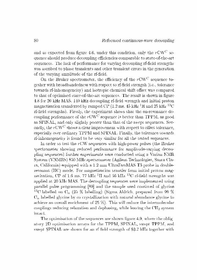
80 Refocused continuous-wave decoupling
and as expected from gure 4.6, under this condition, only the rCWC se-quence should produce decoupling eciencies comparable to state-of-the-artsequences. The lack of performance for varying decoupling rf-eld strengthswas ascribed to phase transients and other transient errors in the generationof the varying amplitude of the rf-eld.
On the Bruker spectrometer, the eciency of the rCWC sequence to-gether with broadbandedness with respect to rf-eld strength (i.e., tolerancetowards rf-inhomogeneity) and isotropic chemical shift oset was comparedto that of optimised state-of-the-art sequences. The result is shown in gure4.8 for 20 kHz MAS, 140 kHz decoupling rf-eld strength and initial protonmagnetisation transferred by ramped CP (1.2 ms, 45 kHz 1H and 25 kHz 13Crf-eld strengths). Firstly, the experiment shows that the on-resonance de-coupling performance of the rCWC sequence is better than TPPM, as goodas SPINAL, and only slightly poorer than that of the swept sequences. Sec-ondly, the rCWC shows a clear improvement with respect to oset tolerance,especially over ordinary TPPM and SPINAL. Finally, the tolerance towardsrf-inhomogeneity is found to be very similar for all the tested sequences.
In order to test the rCW sequences with high-power pulses (the Brukerspectrometer showing reduced performance for amplitude-varying decou-pling sequences) further experiments were conducted using a Varian NMRSystem (VNMRS) 850 MHz spectrometer (Agilent Technologies, Santa Cla-ra, California) equipped with a 1.2 mm UltraFastMAS T3 probe in double-resonant (HC) mode. For magnetisation transfer from initial proton mag-netisation, CP of 1.6 ms, 77 kHz 1H and 56 kHz 13C rf-eld strengths wasapplied at 20 kHz MAS. The decoupling sequences were implemented usingparallel pulse programming [80] and the sample used consisted of glycine13C-labelled on Cα (25 % labelling) (Sigma-Aldrich, prepared from 99 %Cα labelled glycine by co-crystallization with natural abundance glycine toachieve an overall enrichment of 25 %). This will reduce the intermolecularcouplings reducing relaxation and dephasing, while leaving the CH2 systemintact.
The optimisation of the sequences are shown gure 4.9, where the oblig-atory 2D optimisation arrays for the TPPM, SPINAL, swept-TPPM, andswept-SPINAL are shown for an rf-eld strength of 93.7 kHz together with

Performance comparisons 81
SW−TPPM 93.7 kHz
0 10 20
SW−SPINAL 93.7 kHz
0 10 20
Pulse
wid
th /
µs
TPPM 93.7 kHz SPINAL 93.7 kHz
0
0.1
0.2
0.3
0.4
0.5
0.6
0.7
0 10 200 10 20
0 50 100 150 2000
0.5
1
13C
inte
nsity
0 50 100 150 2000 50 100 150 200 0 50 100 150 2000 50 100 150 200
CW rf field strength (kHz)
Phase shift / degrees
ArCW BrCW CrCW DrCW ErCW
CW rf field strength (kHz)
Nu
meri
cal
Exp
eri
men
tal
SW−TPPM 93.7 kHz
0 10 20Phase shift / degrees
SW−SPINAL 93.7 kHz
0 10 20
Pulse
wid
th /
µs
TPPM 93.7 kHz
4.5
5
5.5
6
6.5SPINAL 93.7 kHz
1
1.5
2
2.5
3
3.5
4
0 10 200 10 20
0 50 100 150 2000
2
4
6
Peak
hei
ght /
arb
. uni
ts
0 50 100 150 2000 50 100 150 200 0 50 100 150 2000 50 100 150 200
Peak
hei
ght /
arb
. uni
ts13
C in
tens
ity
ArCW BrCW CrCW DrCW ErCW
4.5
5
5.5
6
6.5
Figure 4.9: Comparison of the optimisation of rCW sequences and of TPPM,SPINAL, swept-TPPM, and swept-SPINAL investigated by simulations and ex-periments for average decoupling rf-eld strength of 93.7 kHz (for rCW 222 kHzpulses and varied CW rf-eld strength). 20 kHz MAS, 850 MHz spectrometerfrequency, 30 ms acquisition, and no apodisation applied. The simulations usedthe CH2 spin system table 4.1, while the experiments were conducted on a 25%13Cα-enriched glycine powder. As measure of the eciency, the 10 ms FID in-tensity was used for simulations, while the Cα-peak height was measured in theexperiments. The red lines indicate 90 kHz CW rf-eld strength, while the greenlines indicate the 70 kHz CW rf-eld strength local optimum. [6] (App. D.1).

82 Refocused continuous-wave decoupling9
3.7
kH
z
ArCW BrCW CrCW DrCW ErCW
70 k
Hz
Figure 4.10: Experimental 13Cα line shape comparison for rCW and state-of-the-art decoupling sequences at 93.7 kHz decoupling average rf-eld strength and atthe local optimum of 70 kHz rf-decoupling obtained for 25% 13Cα-enriched glycine.20 kHz MAS, 850 MHz spectrometer frequency, 30 ms acquisition, and spectraFourier transformed without apodisation. Sequences were individually optimisedas shown gure 4.9. [6] (App. D.1).
plots showing the decoupling performance of the rCW sequences as func-tion of the rf-eld strength (for a pulse strength of 222 kHz which for 90kHz CW gives an average rf-power corresponding to a constant rf-eld of93.7 kHz). At the top of the gure, corresponding simulation results areshown. The rCW sequences show overall smooth increases in decouplingeciency as the rf-eld strength is increased, however, with interesting localoptima. Contrary to this, the other sequences show complicated patternswhich clearly stresses the need for the 2D array optimisation. The main dif-ference between experimental results and those obtained from simulations isthe high experimental eciency of the rCWA which provides equally gooddecoupling as the other rCW sequences. Having optimised the sequences,line shapes are compared for 70 kHz and 93.7 kHz decoupling (indicated bygreen and red lines respectively in gure 4.9) in gure 4.10.
The line shape comparison gure 4.10 shows several remarkable fea-tures. Firstly, the rCW sequences in general perform as good as the other

Performance comparisons 83
sequences at 93.7 kHz, but signicantly better at the local optimum (forthe rCW sequences) at 70 kHz decoupling rf-eld strength. In both cases,the rCWA and rCWC show the best decoupling performance of the rCWsequences which again is ascribed to inferior refocusing performance of theπ-pulses of same phase as the CW eld in which they are incorporatedsince this is the common feature of rCWB, rCWD, and rCWE . The rCWE
sequence fails to show the expected improvement expected from the purg-ing pulses. It is speculated if this could be due to reduced self-decouplingamong the protons [77, 78] since the eect of the purging pulses should beto remove homonuclear dipolar interactions.
Since the analytical results and simulations for the 2-spin system shownear to ideal decoupling for the rCW sequences, diluted spin-systems arethought to be an interesting rCW decoupling application area. Figure 4.11shows 15N-spectra of a sample of 15N-labelled, perdeuterated and 10 %back-exchanged SH3 (Src-homology 3) leaving 10 % of the amide nitrogensprotonated (kindly provided by S. Asami and co-workers [81, 82]). SH3being a small protein domain of 60 residues in a β-barrel fold [83] withstructure determined by solid-state NMR [84], i.e., with a published assign-ment. The spectra are obtained on a Bruker Avance II 700 MHz wide-borespectrometer (Bruker Biospin, Rheinstetten, Germany) equipped with a 2.5mm triple-resonance probe at a MAS frequency of 10 kHz and a decouplingrf-eld strength of 78 kHz (limited by heat sensitivity of the sample). Mag-netisation was transferred from the protons to the nitrogens by a rampedCP (400 µs, 55 kHz 1H, 43 kHz 15N) pulse sequence and rough pulse lengthoptimisations of the decoupling sequences were applied. Due to the low S/N,optimisation of the phase of TPPM, SPINAL, and swept-SPINAL was notpossible (adjusted to 10) which leaves some uncertainty in the nal con-clusions. As evidenced by the spectra a very signicant gain in resolutionand intensities is obtained by the use of the rCW sequences as comparedto ordinary TPPM and SPINAL decoupling. Even compared to the swept-SPINAL considered more robust, use of the rCW sequences increases res-olution substantially. Since focus was on constant-amplitude decoupling,only rCWA, rCWC , and rCWD of the ve rCW sequences were tested. Forthe rst time, experimental results in favour of the more advanced rCWD

84 Refocused continuous-wave decoupling
100105110115120125130135
rCWA
100105110115120125130135
rCWC
100105110115120125130135
δ (15N) / ppm
rCWD
100105110115120125130135
SPINAL64
100105110115120125130135
δ (15N) / ppm
SWf-SPINAL32
100105110115120125130135
TPPM
Figure 4.11: Experimental decoupling eciency comparison for a diluted spin sys-tem of deuterated and 10 % back-exchanged 15N-labelled SH3 showing the amide15N-spectral region under application of dierent decoupling schemes at a constantrf-eld strength of 78 kHz. 10 kHz MAS, 700 MHz spectrometer frequency, 128scans, an acquisition time of 20 ms, and no apodisation applied.

Discussion and conclusion 85
sequence is found. Furthermore, the obtained result stresses the advantageof the rCW sequence of reduced optimisation requirements.
4.4 Discussion and conclusion
Through a thorough average Hamiltonian analysis to third order of CWdecoupling, average Hamiltonians have been identied which explain thepoor decoupling performance of CW decoupling. By the use of togglingframes and semi-continuous BCH, these results have been constructivelyused to signicantly improve the performance of CW decoupling to the levelof, and in some cases beyond, state-of-the-art decoupling sequences. Thishas been done by incorporation of rotor-synchronised π- and π/2-pulses andphase modulation. Good agreement between analytical results, simulationsand experiments has been established which proves the eciency of thedesign principle.
The performance of the dierent rCW sequences follows, in simulations,the analytically expected. However, experimental imperfections such asphase transients together with multi-spin eects such as self-decoupling pre-sumably decrease the expected performance gain expected from the mostadvanced rCW sequences. Especially, incorporation of high-power pulsesduring CW decoupling of the same phase as the pulse proves problematic.Moreover, dierences between spectrometers and less surprising betweensamples are likely to result in dierences in optimum decoupling sequences.
A signicant advantage of the rCW sequences is the very easy optimisa-tion which can be cut down to adjusting the π-pulse length and eventuallyperforming a tiny rf-eld strength optimisation around the desired decou-pling rf-eld strength and a rotor-synchronisation adjustment. This is incomplete contrast to TPPM, SPINAL and even swept versions of thesewhich all require 2D array optimisations for optimal performance. In manycases of samples with inherent low S/N, such an optimisation is close toimpossible which makes the rCW a very attractable alternative.
A speciality for the rCW sequences is the very long averaging periods ofseveral 100 µs. It is speculated that the optimum value for τ ∼ 100 µs which

86 Refocused continuous-wave decoupling
is rather independent of rf-eld strength and MAS frequency (althoughrotor-synchronisation is a requirement) is the result of a lower limit due tonon-preferable interference with MAS averaging and an upper limit whichwill lead to inecient averaging of residual Hamiltonians. Furthermore,these long averaging periods leaves the rCW sequences interesting as meansof decoupling during heterospin manipulations, during which very basicdecoupling schemes are often used to ensure that no unwanted evolutionsoccur.
As judge from analytical results and simulations, the rCW sequencesare supposed to show close to ideal decoupling performance for isolated 2-spin systems. This was examined experimentally by application of the rCWsequences to a diluted spin system with inherent low S/N. For this system,the sequences, indeed, show signicant improvements as compared to ordi-nary TPPM and SPINAL decoupling and even compared to swept-SPINALdecoupling. The inherent low S/N made thorough 2D array optimisationsof the TPPM and SPINAL sequences impossible. A very realistic situation,however, leaving the nal conclusions in this respect with some uncertainty.The high performance found for the rCW sequences applied to a dilutedspin system provides great future prospects for rCW, taking the recent de-velopment in this area [85] into consideration.

Chapter 5
Fluorine decoupling by
refocused continuous-wave
Decoupling is not only relevant in proton containing systems. Other abun-dant nuclei can have similar eects on the neighbouring low-γ nuclei whichcould be objects for NMR investigation. One such abundant nuclei is thenatural occurring isotope of uorine, 19F. Fluorine-19 has many propertiesin common with the proton with respect to NMR: the abundance is 100 %,it is a spin-1/2 nucleus and has similar gyromagnetic ratio (γ(19F)=2.52·108
(Ts)−1 and γ(1H)=2.68·108 (Ts)−1) [86]. However, the isotropic and aniso-tropic chemical shifts dier substantially from those of the proton due to thelarger number of surrounding electrons. Whereas typical values for protonsare 310 ppm for 1H [12], a range of 300 ppm [12, 8792] is not uncommonfor uorine. The chemical shift anisotropy of protons are normally below1015 ppm, again very small compared to 150 ppm and in extreme caseseven 300 ppm [12, 8892] for uorine. The large isotropic chemical shiftdispersion unavoidably leads to large rf-frequency osets for molecules con-taining more than one uorine nuclei (except for isomerism and rotationalaveraging). The large chemical shift anisotropies are most likely not aver-aged completely by MAS at moderate spinning speeds. Both characteristicsof the uorine nucleus aects decoupling eciency dramatically.
87

88 Fluorine decoupling by refocused continuous-wave
During the years, the routine for uorine decoupling has been to applywell-functioning proton decoupling schemes and even standard CW, how-ever, a recent comparative study by Chandran and co-workers [92] elab-orates this further. The most promising decoupling sequences for moder-ate MAS frequencies were compared for decoupling eciency on two rigid,organic, uorine containing molecules, and considerable dierences werefound. In summary, TPPM [63] in general was found to be least ecientand in some cases providing half the intensity of SPINAL64 [47], SWf -TPPM [66], and SWf -(32)-SPINAL32 [67]. Of these three sequences, theswept sequences provided similar and most ecient decoupling. The sweepswere adjusted to (0.91.1) for SPINAL and (0.691.31) for TPPM, however,varying a little for TPPM depending on the molecule.
5.1 Refocused continuous-wave decoupling
On this background it was decided to examine the uorine decoupling per-formance of the rCW [7] (App. D.2) sequences (introduced for protondecoupling chapter 4) since they show tolerance towards isotropic chemicalshift osets and chemical shift anisotropies at moderate MAS frequencies.As such the rCW sequences are strong candidates for uorine decoupling[7].
δiso/ppm ωaniso/2π/kHz ηanisoC 0 0 0F1 0 0120 0F2 5 0120 0
bIS/2π/kHz JIS/HzC-F1 -12.079 235C-F2 -12.079 235F1-F2 -10.410 250
Table 5.1: Spin system parameters for the CF2 3-spin system used for simulationsof the decoupling sequences.

Refocused continuous-wave decoupling 89
Figure 5.1: Amplitudes of the 2nd- and 3rd-order terms of the average Hamiltonianof CW decoupling for a typical 13C-19F spin system as function of chemical shiftanisotropy vs. MAS frequency (left column) and vs. isotropic chemical shift (rightcolumn). A decoupling rf-eld strength of 110 kHz and a dipolar coupling of 12kHz were assumed. The amplitudes are calculated using equations (4.24) and(4.33) as the absolute value averaged over the powder angles. While the scalediers between the plots, the colouring can be used as a reference. Left columnadapted from [7] (App. D.2).
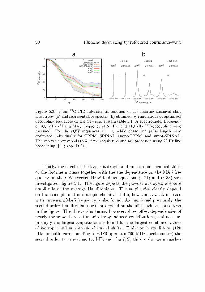
90 Fluorine decoupling by refocused continuous-wave
frequency / Hz
0
0.2
0.4
0.6
0.8
1
0 20 40 60 80 100 120
13C
inte
nsity
19F
= 60 kHz = 120 kHz= 0 kHz
13C
a bTPPM
SPINAL64SWf-TPPM
SWf-SPINAL32rCWA
rCWC
rCWD
-250 0 250
rCWD
-250 0 250-250 0 250
rCWD
-250 0 250
SPINAL64SPINAL64
x1 x6 x6
-250 0 250
rCWD
-250 0 250
SPINAL64
Figure 5.2: 2 ms 13C FID intensity as function of the uorine chemical shiftanisotropy (a) and representative spectra (b) obtained by simulations of optimiseddecoupling sequences on the CF2 spin system table 5.1. A spectrometer frequencyof 700 MHz (1H), a MAS frequency of 5 kHz, and 110 kHz 19F-decoupling wereassumed. For the rCW sequences τ = τr while phase and pulse length wereoptimised individually for TPPM, SPINAL, swept-TPPM, and swept-SPINAL.The spectra corresponds to 51.2 ms acquisition and are processed using 20 Hz linebroadening. [7] (App. D.2).
Firstly, the eect of the larger isotropic and anisotropic chemical shiftsof the uorine nucleus together with the the dependence on the MAS fre-quency on the CW average Hamiltonians equations (4.24) and (4.33) wasinvestigated, gure 5.1. The gure depicts the powder averaged, absoluteamplitude of the average Hamiltonians. The amplitudes clearly dependon the isotropic and anisotropic chemical shifts, however, a weak increasewith increasing MAS frequency is also found. As mentioned previously, thesecond-order Hamiltonian does not depend on the oset which is also seenin the gure. The third-order terms, however, show oset dependencies ofnearly the same sizes as the anisotropy-induced contributions, and not sur-prisingly the largest amplitudes are found for the largest combined valuesof isotropic and anisotropic chemical shifts. Under such conditions (120kHz for both; corresponding to ∼180 ppm at a 700 MHz spectrometer) thesecond-order term reaches 1.5 kHz and the IzSz third-order term reaches

Refocused continuous-wave decoupling 91
4 kHz, while the IySz third-order term stays below 250 Hz (I representingthe uorine and S the low-γ nuclei e.g. carbon-13). As such, these largeaverage Hamiltonians explain that CW decoupling does not suce for u-orine decoupling. Moreover, the importance of eective averaging of theseterms are stressed. The tolerance towards oset as well as chemical shiftanisotropy of the rCW sequences is explained by the very ecient aver-aging of the second-order IxSz and the third-order IzSz terms for all rCWsequences (see section 4.2). This leaves the IySz term for consideration. TherCWA sequence does not average this term which, however, is expected tobe relatively small leaving rCWA an interesting option.
Proceeding to simulations as means of decoupling sequence comparisons,gure 5.2 shows obtained 2 ms 13C FID intensities for three rCW sequencesand individually optimised state-of-the-art decoupling sequences as func-tion of the chemical shift anisotropy of uorine. The simulated spin system(table 5.1 and App. A) corresponds to a 13C19F2 with symmetric uorineCSA tensors and no carbon anisotropy. With this simplied set-up, theinuence of carbon anisotropy was determined by simulation to induce onlyminor changes while a uorine asymmetry ηaniso = 0.5 in general decreasesdecoupling eciency by ∼ 10 % for all sequences. The simulations apply5 kHz MAS, 110 kHz decoupling (constant amplitude), and a spectrometerfrequency of 700 MHz. While phase and pulse lengths were optimised forTPPM, SPINAL, swept-TPPM, and swept-SPINAL, the inter-pulse time ofthe rCW sequences (τ in gure 4.5) were adjusted to 100 µs and refocusing-pulse lengths to π-pulses. Only rCWA, rCWC , and rCWD were includedsince the study focusses on constant amplitude decoupling, being more easilyapplied experimentally. The simulations used the SIMPSON [4143] simu-lation software with the REPULSION [44] scheme (66 αCR, βCR angles and10 γCR angles)
Returning to the results shown in gure 5.2, the increasing uorine CSAevidently challenge the decoupling schemes. Up till anisotropies of 40 kHzonly minor dierences between the decoupling eciencies of the dierentsequences are found. However, while further increases in anisotropy lead tosignicant decreases in decoupling eciencies of all the previously publishedsequences, the impact on all of the rCW sequences certainly is less signi-

92 Fluorine decoupling by refocused continuous-wave
CαF2
CβF2
CγF3
0.5
1
1.5
0.5
1
1
1.5
2
100 110 120
0
0.5
1
1.5
0
0.5
1
0
0.5
1
1.5
2
2.5
-100 -50 0 50 100
pe
ak h
eig
ht
/ a
rb.
un
its
rCWA rCWD
SPINAL64 swf-SPINAL32
rf-amplitude / kHz rf-frequency offset / kHz
CαF2
CβF2
CγF3
Figure 5.3: Experimental comparison of the tolerance towards rf-amplitude (leftcolumn) and rf-frequency oset (right column) of rCWA, rCWD, SPINAL64, andSWf -SPINAL32. The peak heights were extracted from 5 kHz CP/MAS spectraof unlabelled silver heptauorobutyrate (powder sample) using a 700 MHz spec-trometer and 110 kHz decoupling rf-eld strengths. [7] (App. D.2).
cant. This observation is in good agreement with the small IySz term in theaverage Hamiltonian. Together with the 2 ms FID intensities, representa-tive spectra are shown which conrm the advantage of the rCW sequencesat large uorine chemical shift anisotropies.
For experimental testing a rigid, organic chemical compound similar tothat used in the comparative study [92] was used: unlabelled silver hep-tauorobutyrat (97 %, Sigma-Aldrich). The uorines do not represent thelargest uorine chemical shift anisotropies, however, three dierent CFn-groups, n = 2, 3 are present and the molecule constitutes a typical or-ganic peruorinated compound. The silver heptauorobutyrat was rmly

Refocused continuous-wave decoupling 93
CγF3CβF2CαF2
FW
HM
/ H
z
rCWA rCWD
SPINAL64
swf-SPINAL32
MAS frequency / kHz
swf-TPPM
30
40
50
60
70
5 10 15 2030
40
50
60
70
5 10 15 2030
35
40
45
5 10 15 20
Figure 5.4: Experimental performance comparison with respect to MAS frequencyfor rCWA, rCWD, SPINAL64, SWf -SPINAL-32, and SWf -TPPM. FWHM wereextracted from CP/MAS spectra of unlabelled silver heptauorobutyrate (powdersample) using a 700 MHz spectrometer and 110 kHz decoupling rf-eld strengths.The FWHM for SWf -TPPM left out is 62.5 Hz. Adapted from [7] (App. D.2).
grind during sample preparation. A Bruker Avance II 700 MHz wide-borespectrometer (Bruker Biospin. Rheinstetten, Germany) equipped with adedicated 1H-19F-X 2.5 mm triple-resonance probe was used. CP/MAS[45, 46] spectra with dierent decoupling sequences applied during acquisi-tion were acquired using the following optimised parameters (given in theorder: 19F rf-eld, 13C rf-eld, and CP length) and number of scans: 5 kHzMAS: 50 kHz, 45 kHz, 5 ms, 256 scans; 10 kHz MAS: 44 kHz, 53 kHz, 7ms, 32 scans; 20 kHz MAS: 68 kHz, 53 kHz, 5 ms, 256 scans. In all casesan acquisition time of 40 ms was used and no apodisation was applied. Thedecoupling rf-eld strength was adjusted to 110 kHz, and all sequences opti-mised accordingly. For the TPPM-like sequences the optimisation consistedof a 8 by 9 grid in the phase (4 20 in steps of 2) and pulse lengths (3 4.5 µs in steps of 0.25 µs). For the rCW sequences, τ (90110 µs in stepsof 2.5 µs) and the refocusing pulse length (3.25 4.25 µs in steps of 0.25µs, i.e., τπ . 1/(2νrf ) is optimal) were optimised.
After careful optimisations, the tolerance with respect to rf-frequencyoset and rf-eld strength (i.e., the inhomogeneity tolerance) was assayed.The corresponding peak heights for 5 kHz MAS are shown Figure 5.5 for thebest performing sequences. The results obtained for the three carbons (Cα,Cβ , and Cγ) are very similar. The maximum peak height is likewise very

94 Fluorine decoupling by refocused continuous-wave
110115
rCWA
110115
rCWC
110115
rCWD
110115
SPINAL64
110115
SWf-SPINAL32
110115
SWf-TPPM
110115
δ (13
C) / ppm
TPPM
COOAgF
F F
FF
FF
αβγ
γ β α
Figure 5.5: Spectral uorine decoupling eciency comparison in terms of 13CCP/MAS spectra obtained for a powder of silver heptauorobutyrate obtainedusing a 700 MHz NMR spectrometer at 10 kHz MAS. All decoupling sequenceswere applied using a 110 kHz rf-eld strength. [7] (App. D.2).
similar for all sequences, and within the accuracy of the measurements, theon-resonance performance of the sequences are similar, and so are the rf-frequency oset dependencies. On the contrary, the rCW sequences are sig-nicantly less aected by rf-amplitude variations. This clearly contributesto the ease of optimisation of the rCW sequences.
The inuence of the MAS frequency was probed by determination ofthe FWHM (full width at half maximum) for the 13C resonances at MASfrequencies of 5, 10, and 20 kHz. The results for the best performing se-quences are shown gure 5.3. The optimised decoupling eciency of thetwo SPINAL and the swept-TPPM sequences are seen to vary signicantlywith spinning frequency for Cα and Cβ while the eciency is better andmore stable for Cγ (swept-TPPM being an exception). The eciency of therCW sequences does also show dierences for varying spinning frequencies,however, being signicantly more stable for all carbons. The stability ofnearly all sequences for Cγ is ascribed to a lowered anisotropy due to ro-tational motion of the CF3-group. The stability of the rCW sequences forthe CF2-groups is interpreted as evidence of the high performance of thesesequences even for large uorine anisotropies.
As a nal example, the decoupling performance is compared in terms

Conlusion 95
of CP/MAS spectra with 128 scans obtained at 10 kHz MAS, where thebest S/N was achieved. Spectra of all compared sequences are shown gure5.4. The low decoupling eciency of TPPM, described [92], is certainlyconrmed. That said, the patterns from gures 5.3 and 5.4 repeat and thestable high decoupling eciency of the rCW sequences especially for theCF2-groups are seen. The swept-TPPM, which is well-performing at 10kHz MAS, show high eciency as found earlier [92].
5.2 Conlusion
The high decoupling eciency and stability of the rCW sequences, evenat very large chemical shift anisotropies and isotropic chemical shift osetsas is the case for 19F-decoupling, are demonstrated. Under uorine chem-ical shift anisotropies found for ordinary uorinated small molecules, therCW sequences show a high degree of stability towards MAS frequency, rf-amplitude, and spin system in terms of dierent CFn-groups, n = 2, 3. Thestability towards isotropic chemical shift oset is similar to current state-of-the-art sequences (SPINAL64, swept-TPPM, and swept-SPINAL) and thesame holds for the on-resonance performance under optimised conditions.The last point being very important for the SPINAL64, swept-TPPM, andswept-SPINAL sequences which, contrary to the rCW sequences, requirescareful and tedious optimisation. This dierence is a clear advantage infavour of the rCW sequences which can be optimised in a few experiments,here 14 were used (in contrast to 72 for the TPPM-like sequences). Thisadvantage can be crucial for low-sensitivity samples.

96 Fluorine decoupling by refocused continuous-wave

Chapter 6
Conclusions and perspectives
With sensitivity enhancement of MAS solid-state NMR being the focal pointof the projects described in this thesis, important results have been obtainedboth by means of spin-state selection and especially heteronuclear decou-pling. The resolution enhancement projects, aiming at removing line widthcontributions originating from the scalar coupling between CO and Cα, suc-cessfully demonstrated the possibility of manipulations through use of thedipolar coupling. The decoupling development study resulted in high perfor-mance decoupling sequences derived from a thorough average Hamiltoniananalysis approach. This approach resulted in the rCW scheme which showa very broad range of applications.
Dipolar-driven spin-state selection was demonstrated for analyticallyand OC-derived sequences. In the analytical study, the possibility of com-bining dipolar recoupling elements (the EXPORT at two dierent recouplingconditions) in order to achieve a desired spin-manipulation was demon-strated. The combination of the EXPORT elements served to remove theγPR-angle dependency during a transfer of magnetisation from in-phaseto anti-phase magnetisation. A dipolar-driven spin-state selection sequencewas derived and correspondence between analytical results, simulations, andexperiments was established for a 2-spin system, i.e., uniformly 13C-labelledglycine. The transfer time being just around 3 ms is clear testimony to the
97

98 Conclusions and perspectives
use of the stronger dipolar couplings; scalar coupling-based methods using5 ms or even more. The sequence shows moderate experimental eciencywhich is ascribed to inhomogeneity-sensitivity, relaxation eects, and thespread in the transfer rate due to the spread of βPR-angles in a powdersample. These losses could be overcome since the sequence is applicable inregimes, where scalar coupling-based sequences are hindered due to theirdependence on high-power 1H-decoupling. However, dysfunction is foundfor larger spin systems. This issue was addressed by the improved spin-stateselective excitation sequence presented which, according to simulations, suc-cessfully applies to larger spin systems. The experimental incorporation is,however, hampered by the use of selective Cβ-pulses, and future work shoulddenitely address the outlined implementation using CO-selective pulses in-stead.
The OC spin-state selection sequences show capability of achieving spin-state selection in only 2 ms again due to the use of the strong dipolar cou-pling as means of magnetisation transfer. The sequences reach the theoret-ical transfer bounds according to simulations and around 80 % experimen-tally for uniformly 13C-labelled glycine. Similar to the analytically derivedsequences, successful implementation of the OC-based sequences on largerspin-systems have not been achieved. The main reason is expected to bethe sensitivity towards spin-system geometry and future work will addressthis issue by optimisation over a broader range of spin-system geometriesin terms of the dipolar βPC- and γPC-angles. A clear advantage of the OC-approach is that the spin-state selection is achieved in one scan and higheciencies are achievable.
The rCW decoupling scheme, derived from an average Hamiltoniananalysis of CW decoupling, is presented as an easily implementable, high-performing, broadly applicable means of heteronuclear decoupling. Thesequence applies to decoupling of abundant spins facilitating acquisitionof high-resolution solid-state CP/MAS NMR spectra of low-γ nuclei. Theperformance is shown to be similar to or in some cases even better thanstate-of-the-art sequences represented by TPPM, SPINAL, and swept ver-sions of these. The rCW scheme developed for proton decoupling hasbeen shown robust towards rf-inhomogeneity, -amplitude variations, and

99
-frequency osets as well as large chemical shift anisotropies. These char-acteristics, combined with ease of implementation and optimisation, makethe rCW scheme broadly applicable which has been demonstrated by thestable state-of-the-art uorine decoupling performance. Furthermore, veryhigh decoupling eciency has been found for diluted spin systems provid-ing excellent prospects for the rCW scheme given the recent developmentof NMR on diluted spin systems.

100 Conclusions and perspectives

Bibliography
[1] E. R. Andrew, A. Bradbury, R. G. Eades, Nuclear Magnetic Res-onance Spectra from a Crystal rotated at High Speed, Nature 182(1958) 1659.
[2] I. J. Lowe, Free Induction Decays of Rotating Solids, Phys. Rev.Lett. 2 (1959) 285287.
[3] S. K. Straus, T. Bremi, R. R. Ernst, Resolution enhancement byhomonuclear J decoupling in solid-state MAS NMR, Chem. Phys.Lett. 262 (1996) 709715.
[4] L. Chen, R. A. Olsen, D. W. Elliott, J. M. Boettcher, D. H. Zhou,C. M. Rienstra, L. J. Mueller, Constant-Time Through-Bond 13C Cor-relation Spectroscopy for Assigning Protein Resonances with Solid-State NMR Spectroscopy, J. Am. Chem. Soc. 128 (2006) 99929993.
[5] C. Kehlet, J. T. Nielsen, Z. To²ner, N. C. Nielsen, Resolution-Enhanced Solid-State NMR 13C-13C Correlation Spectroscopy by Op-timal Control Dipolar-Driven Spin-State-Selective Coherence Trans-fer, J. Phys. Chem. Lett. 2 (2011) 543547.
[6] J. M. Vinther, A. B. Nielsen, M. Bjerring, E. R. H. van Eck, A. P. M.Kentgens, N. Khaneja, N. C. Nielsen, Refocused continuous-wavedecoupling: A new approach to heteronuclear dipolar decoupling insolid-state NMR spectroscopy, J. Chem. Phys. (2012). Submitted.
101

102 BIBLIOGRAPHY
[7] J. M. Vinther, N. Khaneja, N. C. Nielsen, Robust and Ecient 19FHeteronuclear Dipolar Decoupling using Refocused Continuous-WaveRf Irradiation, J. Magn. Reson. (2012). Submitted.
[8] F. Bloch, W. W. Hansen, M. Packard, Nuclear Induction, Phys. Rev.69 (1946) 127127.
[9] F. Bloch, Nuclear Induction, Phys. Rev. 70 (1946) 460474.
[10] E. M. Purcell, H. C. Torrey, R. V. Pound, Resonance Absorption byNuclear Magnetic Moments in a Solid, Phys. Rev. 69 (1946) 3738.
[11] J. M. Vinther, N. C. Nielsen, Notes on NMR spectroscopy: an in-troduction to the principles of NMR spectroscopy, InterdisciplinaryNanoscience Center (iNANO) and Department of Chemistry, AarhusUniversity, 2012.
[12] M. Mehring, High Resolution NMR in Solids, Springer-Verlag NewYork, 1976.
[13] K. Schmidt-Rohr, H. W. Spiess, Multidimensional solid-state nmr andpolymers, Academic Press, 1994.
[14] N. C. Nielsen, Forelæsningsnoter i faststof NMR spektroskopi, AarhusUniversitet, 1997.
[15] W. Magnus, On the Exponential Solution of Dierential Equationsfor a Linear Operator, Commun. Pure Appl. Math. 7 (1954) 649673.
[16] D. P. Burum, Magnus expansion generator, Phys. Rev. B 24 (1981)36843692.
[17] M. Hohwy, N. C. Nielsen, Systematic design and evaluationof multiple-pulse experiments in nuclear magnetic resonance spec-troscopy using a semi-continuous Baker-Campbell-Hausdor expan-sion, J. Chem. Phys. 109 (1998) 3780.

BIBLIOGRAPHY 103
[18] D. P. Burum, W. K. Rhim, Analysis of multiple pulse NMR in solids.III, J. Phys. Chem. 71 (1979) 944956.
[19] J. J. Sakurai, Modern Quantum Mechanics, Addison Wesley, 1994.
[20] E. Wigner, Gruppentheorie und ihre Anwendung auf die Quanten-mechanik der Atomspektren, Vieweg : Braunschweig, 1931.
[21] V. Chevelkov, Z. Chen, W. Bermel, B. Reif, Resolution enhancementin MAS solid-state NMR by application of 13C homonuclear scalardecoupling during acquisition, J. Magn. Reson. 172 (2005) 5662.
[22] L. Duma, S. Hediger, B. Brutscher, A. Böckmann, L. Emsley, Resolu-tion enhancement in multidimensional solid-state NMR spectroscopyof proteins using spin-state selection, J. Am. Chem. Soc. 125 (2003)1181611817.
[23] L. Duma, S. Hediger, A. Lesage, L. Emsley, Spin-state selection insolid-state NMR, J. Magn. Reson. 164 (2003) 187195.
[24] R. Verel, T. Manolikas, A. B. Siemer, B. H. Meier, Improved resolu-tion in 13C solid-state spectra through spin-state-selection, J. Magn.Reson. 184 (2007) 322329.
[25] S. Laage, A. Lesage, L. Emsley, I. Bertini, I. C. Felli, R. Pierat-telli, G. Pintacuda, Transverse-Dephasing Optimized HomonuclearJ-Decoupling in Solid-State NMR Spectroscopy of Uniformly 13C-Labeled Proteins, J. Am. Chem. Soc. 131 (2009) 1081610817.
[26] I. Scholz, S. Jehle, P. Schmieder, M. Hiller, F. Eisenmenger, H. Os-chkinat, B.-J. van Rossum, J-deconvolution using maximum entropyreconstruction applied to 13C-13C solid-state cross-polarization magic-angle-spinning NMR of proteins, J. Am. Chem. Soc. 129 (2007) 66826683.
[27] S. R. Hartmann, E. L. Hahn, Nuclear Double Resonance in the Ro-tating Frame, Phys. Rev. 128 (1962) 20422053.

104 BIBLIOGRAPHY
[28] A. Bax, R. Freeman, S. P. Kempsell, Natural abundance carbon-13-carbon-13 coupling observed via double-quantum coherence, J. Am.Chem. Soc. 102 (1980) 48494851.
[29] N. C. Nielsen, H. Thøgersen, O. W. Sørensen, Doubling the Sensitivityof INADEQUATE for Tracing Out the Carbon Skeleton of Moleculesby NMR, J. Am. Chem. Soc. 117 (1995) 1136511366.
[30] N. C. Nielsen, H. Thøgersen, O. W. Sørensen, A systematic strat-egy for design of optimum coherent experiments applied to ecientinterconversion of double- and single-quantum coherences in nuclearmagnetic resonance, J. Chem. Phys. 105 (1996) 39623968.
[31] A. Meissner, J. O. Duus, O. W. Sørensen, Integration of spin-state-selective excitation into 2D NMR correlation experiments with theheteronuclear ZQ/2Q π rotations for 1JXH-resolved E.COSY-typemeasurements of heteronuclear coupling constants in proteins, J.Biomol. NMR 10 (1997) 8994.
[32] M. D. Sørensen, A. Meissner, O. W. Sørensen, Spin-state-selectivecoherence transfer via intermediate states of two-spin coherence in ISspin systems: Application to E.COSY-type measurement of J couplingconstants, J. Biomol. NMR 10 (1997) 181186.
[33] J. A. Stringer, C. E. Bronnimann, C. G. Mullen, D. H. Zhou, S. A.Stellfox, Y. Li, E. H. Williams, C. M. Rienstra, Reduction of RF-induced sample heating with a scroll coil resonator structure for solid-state NMR probes, J. Magn. Reson. 173 (2005) 4048.
[34] F. D. Doty, J. Kulkarni, C. Turner, G. Entzminger, A. Bielecki, Us-ing a cross-coil to reduce RF heating by an order of magnitude intriple-resonance multinuclear MAS at high elds, J. Magn. Reson.182 (2006) 239253.
[35] P. L. Gor'kov, E. Y. Chekmenev, C. Li, M. Cotten, J. J. Buy, N. J.Traaseth, G. Veglia, W. W. Brey, Using low-E resonators to reduce

BIBLIOGRAPHY 105
RF heating in biological samples for static solid-state NMR up to 900MHz, J. Magn. Reson. 185 (2007) 7793.
[36] B. Dillmann, K. Elbayed, H. Zeiger, M.-C. Weingertner, M. Piotto,F. Engelke, A novel low-E eld coil to minimize heating of biologi-cal samples in solid-state multinuclear NMR experiments, J. Magn.Reson. 187 (2007) 1018.
[37] A. L. Webber, A. J. Pell, E. Barbet-Massin, M. J. Knight, I. Bertini,I. C. Felli, R. Pierattelli, L. Emsley, A. Lesage, G. Pintacuda,Combination of DQ and ZQ coherences for sensitive through-bondNMR correlation experiments in biosolids under ultra-fast MAS,ChemPhysChem 13 (2012) 24052411.
[38] A. B. Nielsen, L. A. Straasø, A. J. Nieuwkoop, C. M. Rienstra,M. Bjerring, N. C. Nielsen, Broadband Heteronuclear Solid-StateNMR Experiments by Exponentially Modulated Dipolar Recouplingwithout Decoupling, J. Phys. Chem. Lett. 1 (2010) 19521956.
[39] J. Lin, M. J. Bayro, R. G. Grin, N. Khaneja, Dipolar recouplingin solid state NMR by phase alternating pulse sequences, J. Magn.Reson. 197 (2009) 145152.
[40] M. Bak, R. Schultz, T. Vosegaard, N. C. Nielsen, Specication andvisualization of anisotropic interaction tensors in polypeptides andnumerical simulations in biological solid-state NMR, J. Magn. Reson.154 (2002) 2845.
[41] M. Bak, J. T. Rasmussen, N. C. Nielsen, SIMPSON: a general sim-ulation program for solid-state NMR spectroscopy, J. Magn. Reson.147 (2000) 296330.
[42] T. Vosegaard, A. Malmendal, N. C. Nielsen, The Flexibility of SIMP-SON and SIMMOL for Numerical Simulations in Solid- and Liquid-State NMR Spectroscopy, Monatsh. Chem. 133 (2002) 15551574.

106 BIBLIOGRAPHY
[43] Z. To²ner, T. Vosegaard, C. Kehlet, N. Khaneja, S. J. Glaser, N. C.Nielsen, Optimal control in NMR spectroscopy: numerical implemen-tation in SIMPSON, J. Magn. Reson. 197 (2009) 120134.
[44] M. Bak, N. C. Nielsen, REPULSION, A Novel Approach to EcientPowder Averaging in Solid-State NMR, J. Magn. Reson. 125 (1997)132139.
[45] A. Pines, M. G. Gibby, J. S. Waugh, Proton-enhanced NMR of dilutespins in solids, J. Phys. Chem. 59 (1973) 569590.
[46] G. Metz, X. Wu, S. Smith, Ramped-Amplitude Cross Polarizationin Magic-Angle-Spinning NMR, J. Magn. Reson. Ser. A 110 (1994)219227.
[47] B. M. Fung, A. K. Khitrin, K. Ermolaev, An improved broadbanddecoupling sequence for liquid crystals and solids, J. Magn. Reson.142 (2000) 97101.
[48] G. Cornilescu, J. L. Marquardt, M. Ottiger, A. Bax, Validation ofProtein Structure from Anisotropic Carbonyl Chemical Shifts in aDilute Liquid Crystalline Phase, J. Am. Chem. Soc. 120 (1998) 6836.
[49] J. Cavanagh, W. J. Fairbrother, A. G. P. III, N. J. Skelton, M. Rance,Protein NMR Spectroscopy, Principles and Practice, Academic Press,2007.
[50] N. Khaneja, N. C. Nielsen, Triple oscillating eld technique for accu-rate distance measurements by solid-state NMR, J. Chem. Phys. 128(2008) 015103.
[51] N. Khaneja, T. Reiss, C. Kehlet, T. Schulte-Herbrüggen, S. J. Glaser,Optimal control of coupled spin dynamics: design of NMR pulse se-quences by gradient ascent algorithms, J. Magn. Reson. 172 (2005)296305.

BIBLIOGRAPHY 107
[52] D. Wei, U. Akbey, B. Paaske, H. Oschkinat, B. Reif, M. Bjerring,N. C. Nielsen, Optimal 2H Rf Pulses and 2H-13C Cross-PolarizationMethods for Solid-State 2H MAS NMR of Perdeuterated Proteins, J.Phys. Chem. Lett. 2 (2011) 12891294.
[53] O. W. Sørensen, Polarisation transfer experiments in high-resolutionNMR spectroscopy, Prog. NMR Spectrosc. 21 (1989) 503569.
[54] O. W. Sørensen, A Universal Bound on Spin Dynamics, J. Mag.Reson. 86 (1990) 435440.
[55] K. Takegoshi, S. Nakamura, T. Terao, 13C1H dipolar-assisted rota-tional resonance in magic-angle spinning NMR, Chem. Phys. Lett.344 (2001) 631637.
[56] E. Brunner, D. Fenzke, D. Freude, H. Pfeifer, The inuence ofhomonuclear dipolar interaction on the residual linewidths of MASNMR spectra, Chem. Phys. Lett. 169 (1990) 591594.
[57] Y. K. Lee, N. D. Kurur, M. Helmle, O. G. Johannessen, N. C. Nielsen,M. Levitt, Ecient dipolar recoupling in the NMR of rotating solids.A sevenfold symmetric radiofrequency pulse sequence, Chem. Phys.Lett. 242 (1995) 304309.
[58] M. H. Levitt, Symmetry in the design of NMR multiple-pulse se-quences, J. Chem. Phys. 128 (2008) 052205.
[59] M. H. Levitt, R. Freeman, NMR Population Inversion Using a Com-posite Pulse, J. Magn. Reson. 33 (1979) 473.
[60] M. H. Levitt, R. Freeman, Composite Pulse Decoupling, J. Magn.Reson. 43 (1981) 502.
[61] J. S. Waugh, Theory of broadband spin decoupling, J. Magn. Reson.50 (1982) 3049.

108 BIBLIOGRAPHY
[62] G. D. Paëpe, P. Hodgkinson, L. Emsley, Improved heteronuclear de-coupling schemes for solid-state magic angle spinning NMR by directspectral optimization, Chem. Phys. Lett. 376 (2003) 259267.
[63] A. E. Bennett, C. M. Rienstra, M. Auger, K. V. Lakshmi, R. G.Grin, Heteronuclear decoupling in rotating solids, J. Chem. Phys.103 (1995) 69516958.
[64] A. Detken, E. H. Hardy, M. Ernst, B. H. Meier, Simple and ecientdecoupling in magic-angle spinning solid-state NMR: the XiX scheme,Chem. Phys. Lett. 356 (2002) 298304.
[65] M. Weingarth, G. Bodenhausen, P. Tekely, Low-power decoupling athigh spinning frequencies in high static elds, J. Magn. Reson. 199(2009) 238241.
[66] C. V. Chandran, P. K. Madhu, N. D. Kurur, T. Bräuniger, Swept-frequency two-pulse phase modulation (SWf -TPPM) sequences withlinear sweep prole for heteronuclear decoupling in solid-state NMR,Magn. Reson. Chem. 46 (2008) 943947.
[67] C. V. Chandran, T. Bräuniger, Ecient heteronuclear dipolar decou-pling in solid-state NMR using frequency-swept SPINAL sequences,J. Magn. Reson. 200 (2009) 226232.
[68] C. Augustine, N. D. Kurur, Supercycled SWf -TPPM sequence forheteronuclear dipolar decoupling in solid-state nuclear magnetic res-onance, J. Magn. Reson. 209 (2011) 156160.
[69] S. Paul, N. D. Kurur, P. K. Madhu, On the choice of heteronucleardipolar decoupling scheme in solid-state NMR, J. Magn. Reson. 207(2010) 140148.
[70] R. W. Martin, K. W. Zilm, Preparation of protein nanocrystals andtheir characterization by solid state NMR, J. Magn. Reson. 165 (2003)162174.

BIBLIOGRAPHY 109
[71] P. C. A. van der Wel, J. R. Lewandowski, R. G. Grin, Solid-StateNMR Study of Amyloid Nanocrystals and Fibrils Formed by the Pep-tide GNNQQNY from Yeast Prion Protein Sup35p, J. Am. Chem.Soc. 129 (2007) 51175130.
[72] L. Sperling, A. Nieuwkoop, A. Lipton, D. Berthold, C. Rienstra, Highresolution NMR spectroscopy of nanocrystalline proteins at ultra-highmagnetic eld, J. Biomol. NMR 46 (2010) 149155.
[73] S. K. Vasa, H. Janssen, E. R. H. V. Eck, A. P. M. Kentgens, High-resolution solid-state 13C MAS NMR with long coherence life times,Phys. Chem. Chem. Phys. 13 (2011) 104106.
[74] M. Ernst, Heteronuclear spin decoupling in solid-state NMR undermagic-angle sample spinning, J. Magn. Reson. 162 (2003) 134.
[75] A. Abragam, J. Winter, Quelques expérimences sur la forme des raiesde résonances en réseau rigide, C. r. hebd. séances Acad. sci. 249(1959) 1633.
[76] A. Abragam, Principles of Nuclear Magnetism, Clarendon Press, 1961.
[77] M. Eden, M. H. Levitt, Pulse sequence symmetries in the nuclearmagnetic resonance of spinning solids: Application to heteronucleardecoupling, J. Chem. Phys. 111 (1999) 15111519.
[78] G. D. Paëpe, B. Elena, L. Emsley, Characterization of heteronucleardecoupling through proton spin dynamics in solid-state nuclear mag-netic resonance spectroscopy, J. Phys. Chem. 121 (2004) 31653180.
[79] M. Ernst, A. Samoson, B. H. Meier, Decoupling and recoupling usingcontinuous-wave irradiation in magic-angle-spinning solid-state NMR:a unied description using bimodal Floquet theory, J. Chem. Phys.123 (2005) 64102.
[80] D. Rice, Parallel Programming, Agilent Technologies, Santa Clara,CA 95051 USA, 2011. Text for Chapters 2 and 3 of the User Pro-gramming Manual based on Dan Iverson's Input.

110 BIBLIOGRAPHY
[81] V. Chevelkov, K. Rehbein, A. Diehl, B. Reif, Ultrahigh resolutionin proton solid-state NMR spectroscopy at high levels of deuteration,Angew Chem Int Ed Engl 45 (2006) 38783881.
[82] S. Asami, P. Schmieder, B. Reif, High resolution 1H-detected solid-state NMR spectroscopy of protein aliphatic resonances: access totertiary structure information, J Am Chem Soc 132 (2010) 1513315135.
[83] A. Musacchio, M. Noble, R. Pauptit, R. Wierenga, M. Saraste, Crystalstructure of a Src-homology 3 (SH3) domain, Nature 359 (1992) 851855.
[84] F. Castellani, B. van Rossum, A. Diehl, M. Schubert, K. Rehbein,H. Oschkinat, Structure of a protein determined by solid-state magic-angle-spinning NMR spectroscopy, Nature 420 (2002) 98102.
[85] B. Reif, Ultra-high resolution in MAS solid-state NMR of perdeuter-ated proteins: Implications for structure and dynamics, J. Magn.Reson. 216 (2012) 112.
[86] D. R. Lide, CRC Handbook of Chemistry and Physics, CRC Press,1998.
[87] B. R. Appleman, B. P. Dailey, Fluorine shielding anisotrophy inCFCl3, J. Magn. Reson. 16 (1974) 265273.
[88] M. Mehring, R. G. Grin, J. S. Waugh, 19F Shielding Tensors fromCoherently Narrowed NMR Powder Spectra, J. Chem. Phys. 55 (1971)746.
[89] A. B. Harris, E. Hunt, H. Meyer, Anisotropy of the 19F ChemicalShift of Trapped CHF3 and NF3, J. Chem. Phys. 42 (1965) 2851.
[90] U. H. Dürr, S. L. Grage, R. Witter, A. S. Ulrich, Solid state 19FNMR parameters of uorine-labeled amino acids. Part I: Aromaticsubstituents, J. Magn. Reson. 191 (2008) 715.

BIBLIOGRAPHY 111
[91] S. L. Grage, U. H. Dürr, S. Afonin, P. K. Mikhailiuk, I. V. Komarov,A. S. Ulrich, Solid state 19F NMR parameters of uorine-labeledamino acids. Part II: Aliphatic substituents, J. Magn. Reson. 191(2008) 1623.
[92] C. V. Chandran, P. K. Madhu, P. Wormald, T. Bräuniger, Frequency-swept pulse sequences for 19F heteronuclear spin decoupling in solid-state NMR, J. Magn. Reson. 206 (2010) 255263.
[93] R. K. Harris, E. D. Becker, S. M. C. de Menezes, P. Granger, R. E.Homan, K. W. Zilm, Further conventions for NMR shielding andchemical shifts, Pure Appl. Chem. 80 (2008) 5984.
[94] D. M. Grant, Chemical Shift Tensors, John Wiley & Sons, Ltd.
[95] C. H. Ye, R. Q. Fu, J. Z. Hu, L. Hou, S. W. Ding, Carbon-13 chemicalshift anisotropies of solid amino acids, Magn. Reson. Chem. 31 (1993)699704.
[96] Y. Wei, D.-K. Lee, A. Ramamoorthy, Solid-State 13C NMR ChemicalShift Anisotropy Tensors of Polypeptides, J. Am. Chem. Soc. 123(2001) 61186126.
[97] D. O'Hagan, Understanding organouorine chemistry. An introduc-tion to the C-F bond, Chem. Soc. Rev. 37 (2008) 308319.
[98] W. R. Dolbier, Guide to Fluorine NMR for Organic Chemists, Wiley,2009.
[99] Pulse Programming, Bruker BioSpin GmbH, D-76287 Rheinstetten,Germany, version 2.1.1 edition, 2008.
[100] J. D. van Beek, matNMR: a exible toolbox for processing, analyzingand visualizing magnetic resonance data in Matlab, J. Magn. Reson.187 (2007) 1926.

112 BIBLIOGRAPHY
Appendix A
Design of spin systems for
simulations
The rst step in simulating an NMR experiment should always be to con-struct a trustworthy spin system suitable for the actual problem since allresults from the simulations depend crucially on the spin system. This isperhaps evident, however, lack of knowledge often hinders this point. In thisappendix the approachs used during the work on the projects for designingthe right spin systems is summarised.
Three steps have been identied as crucial for designing a trustworthyspin system: 1) gathering of information / data needed, 2) calculating andprogramming of the data into a spin system, and 3) verication of theprogrammed spin system.
The rst step divides into two subcategories: a literature study and ahomogenisation of the data since several dierent conventions for represen-tation of CSAs have been used during the years. The conversion is addressedin section A.1. The second step involves calculating the Euler angles (sec-tion A.2). The third step has been solved by programming of a script whichprovides visualisations of the programmed spin system (section A.3)
113

114 Design of spin systems for simulations
A.1 Conventions and conversions
Three dierent conventions for the chemical shielding tensor are widely used[93], whereof the "Mehring" and the "Haeberlen" are summarised here andrelated to the convention used in the SIMPSON [4143] simulation softwareused in this work.
σ22
σ11 σ33
σyy
σxx σzz
δ22
δ11 δ33
δyy
δxx δzz
A
σ22
σ11 σ33
σyy
σzz σxx
δ22
δ11 δ33
δyy
δzz δxx
B
Shielding
Shift
Figure A.1: The shielding and shift conventions in two cases. The dierence inthe "letter" conventions between case A and B is noticed.
The "Mehring" convention uses
σ11 ≤ σ22 ≤ σ33, (A.1)
where σii is a diagonal component of the shielding tensor in the PAS.The "Haeberlen" convention uses
|σzz − σiso| ≥ |σxx − σiso| ≥ |σyy − σiso|, (A.2)
where σii is a diagonal component of the shielding tensor in the PAS, how-ever, the ordering depends on the absolute value of the dierence between

Conventions and conversions 115
σii and the isotropic chemical shielding σiso given by
σiso = 13(σxx + σyy + σzz). (A.3)
Two conventions applies for the shielding anisotropy
∆σ = σzz − 12(σxx + σyy) and ζ = σzz − σiso, (A.4)
however, they are easily converted
∆σ = 32ζ. (A.5)
The shielding asymmetry is given by
η =σyy − σxx
ζ. (A.6)
Another approach is to give the shift instead of the shielding. This isdone by Grant [94] as follows
δ11 ≥ δ22 ≥ δ33. (A.7)
However, in SIMPSON [4143] the shift is given by the isotropic shift
δiso = 13(δxx + δyy + δzz), (A.8)
the anisotropic shiftδaniso = δzz − δiso, (A.9)
and the anisotropy
ηaniso =δyy − δxxδaniso
, (A.10)
according to|δzz − δiso| ≥ |δxx − δiso| ≥ |δyy − δiso|. (A.11)
To convert chemical shielding tensors for use in SIMPSON spin systemsthe following conversion formulas are derived.

116 Design of spin systems for simulations
For all conventions the isotropic value is the average of the three shield-ings or shifts
xiso = 13
∑xii, (A.12)
and the shift is equal to the negative of the shielding
δii = −σii. (A.13)
The shift anisotropy is obtained from the shielding anisotropy by
δaniso = −ζ = −23∆σ, (A.14)
sinceδaniso ≡ δzz − δiso = −(σzz − σiso) ≡ −ζ, (A.15)
and the asymmetry is equally well calculated from the shift as from theshieldings
ηaniso =δyy − δxxδaniso
=−(σyy − σxx)
−ζ =σyy − σxx
ζ= η. (A.16)
The problem to convert between the "letter" conventions and the "num-ber" conventions, however, remains and can only be carried out given thespecic values and using the equations (A.1) and (A.2) for the shielding and(A.7) and (A.8) for the shifts. This is exemplied in gure A.1.
A.2 Calculation of Euler angles
The Euler angles of the tensors of the spin system describe the transfor-mation of the tensor into the crystal frame. This means that when a spinsystem is constructed, i.e., the orientation of the tensors are determined,the Euler angles have to be converted to the reverse transformation. Thatis, the Euler angles (α′, β′, and γ′) to turn each ellipsoid (coordinate sys-tem of the tensor) from a common initial position to the desired position.Afterwards, the Euler angles for the reverse transformation (α, β, and γ)are determined:
α = −γ′, β = −β′, and γ = −α′. (A.17)
For reference, the Euler angles are shown gure A.2.

Visualising the spin system 117
x
y
z
z'
x'
y'α
β
γ
Figure A.2: The Euler angles involved in transferring frame xyz to x′y′z′.
A.3 Visualising the spin system
A visualisation script has been written in order to check the calculated Eulerangles and the consistency of the constructed spin system. Furthermore, thescript can be used to assist envisaging a given spin system.
The script calculates the position of the spins using the size and tensororientation of certain dipolar couplings (incorporated for proton, carbon,nitrogen, and uorine). Secondly, it depicts the absolute values of the ten-sors of the CSA and the dipolar couplings as ellipsoids (optionally with acoordinate system) in the position of the spin and in the middle betweenthe involved spins, respectively. Connections between each spin is drawnas guiding lines. The adjustable parameters are: the size factors for theCSA and dipolar coupling tensors, the colouring of the CSA tensors, thecentre spin, the size of the spheres representing spins without CSA, and thespectrometer frequency (which aects the size of the CSA tensors). Fur-thermore, the dipolar couplings used for the positioning of the spins can bechosen.
Figure A.3 shows a typical example of the output of the script. Fur-thermore, the gure illustrates a typical error in a spin system: A glycine

118 Design of spin systems for simulations
Figure A.3: A visualisation of an alanine 13C-labelled spin system (only carbonatoms) showing a typical error: at least the Euler angles of one dipolar couplingtensor has been wrongly calculated. Dipolar coupling tensors: blue, aliphaticcarbon: red, carbonyl carbon: green.
carbon-13 spin system has been tried expanded to an alanine carbon-13 spinsystem, however, the Euler angles of the dipolar couplings to the added Cβdoes not match the Euler angles of the coupling between the Cα and theCO.
Figure A.4 shows the script in use as a help to envisage a spin system [41]consisting of a carbon-13 and three protons in a CH2(C)H conformation.The gure reveals a surprising choice of the Euler angles of the bottom-left proton CSA tensor since it is normally assumed that the tensors pointtowards the carbon atom. Furthermore, it shows that a at structure, i.e.,a double bond structure has been chosen. Such results are very dicult toobtain without a tool for visualisation of the spin systems.
A.4 The applied spin systems
This section shows the applied spin systems for simulations of NMR exper-iments for the dierent projects described in this thesis.

The applied spin systems 119
Figure A.4: A visualisation of a CH2-(C)H13C-labelled spin system from [41]
showing a surprising choice of the Euler angles of the bottom-left proton CSAtensor. Dipolar coupling tensors: blue, carbon: red, proton: green.
A.4.1 Resolution enhancement
For the resolution enhancement project aiming at removing the splitting ofthe carbonyl carbon due to the scalar coupling to the Cα a carbon-13 2-spin system has been designed based on the typical amino acid parametersfor CO and Cα shift tensors, dipolar and scalar coupling given in [40]. Forexperimental testing, 13C-labelled glycine has been used for which slightlydierent values have been reported: for the Cα δaniso = 30 ± 12 ppm andηaniso = 0.75 [95] has been reported and the values dier for the dierentamino acids; δaniso : 2032 ppm and ηaniso : 0.8-1.0 [96]. Keeping thisdierence in mind it was, however, decided to use the typical values sincethe goal is to develop generally applicable sequences. The spin system isgiven below as SIMPSON [4143] input and visualised in gure A.5.
spinsys
channels 13C
nuclei 13C 13C
shift 1 170p -76p 0.90 0 0 94
shift 2 50p -20p 0.43 90 90 0
dipole 1 2 -2142 0 90 120.8
jcoupling 1 2 55 0 0 0 0 0

120 Design of spin systems for simulations
Figure A.5: A visualisation of the 13C-labelled CO-Cα 2-spin system based on thetypical values given in Ref. [40]. Dipolar coupling tensors: blue, aliphatic carbon:red, carbonyl carbon: green.
To test the eect of a longer carbon chain, SIMMOL [40] was usedto generate a CO-Cα-Cβ-Cγ spin system. The spin system is constructedusing the geometry of residue 15 in Ubiquitin, pdb 1D3Z [48]. The isotropicchemical shift has been changed for generally reported leucine chemicalshifts and similarly the scalar couplings have been adjusted. The SIMPSONinput is given below and the system is visualised in gure A.6.
spinsys
channels 13C
nuclei 13C 13C 13C 13C
shift 1 174p -76p 0.9 15.543 3.9072 46.228
shift 2 53p -20p 0.43 86.172 90.781 -32.255
shift 3 40p -20p 0.43 101.54 3.9072 46.228
shift 4 25p -20p 0.43 101.54 3.9072 46.228
dipole 2 1 -2145.1 0 92.399 92.405
dipole 2 3 -2016.7 0 161.93 -94.919
dipole 2 4 -405.7 0 130.52 -82.052
dipole 1 3 -515.11 0 125.25 -89.356

The applied spin systems 121
Figure A.6: A visualisation of the 4-spin system carbon chain based on a 13C-labelled leucine spin system. The system is constructed using SIMMOL [40] andthe geometry of residue 15 in Ubiquitin, pdb 1D3Z [48]. Dipolar coupling tensors:blue, aliphatic carbon: red, carbonyl carbon: green.
dipole 1 4 -127.26 0 115.16 -84.435
dipole 3 4 -1958.8 0 99.014 -78.08
jcoupling 2 1 55 0 0 0 0 0
jcoupling 2 3 35 0 0 0 0 0
jcoupling 3 4 35 0 0 0 0 0
A third spin system, slightly diering from the typical CO-Cα 2-spin sys-tem, has been used for the optimal control based development of spin-stateselection sequences. The system is based on the values used for developmentof the DDOCS3CT sequence [5]. The orientation of the dipolar couplingand the Cα shift tensor with respect to the CO shift tensor diers slightlyfrom the typical orientation [40]. The two spin systems are shown in g.A.7 and the SIMPSON input is given below.
spinsys
channels 13C
nuclei 13C 13C
shift 1 170p -76p 0.90 0 0 94

122 Design of spin systems for simulations
Figure A.7: Comparison of the 13C-labelled CO-Cα 2-spin system based on Ref.[40] (left) and the system based on Ref. [5] (right). The orientation of the dipolarcoupling and the Cα shift tensor with respect to the larger CO shift tensor is seento dier. Dipolar coupling tensors: blue, aliphatic carbon: red, carbonyl carbon:green.
shift 2 50p -20p 0.43 90 90 0
dipole 1 2 -2142 0 0 0
jcoupling 1 2 55 0 0 0 0 0
A.4.2 Proton decoupling
The spin systems used for the proton decoupling simulations have beenconstructed using a tetrahedral geometry of protons around a carbon atomeventually with an extra remote proton resembling a proton on a neighbour-ing aliphatic carbon atom. The dipolar coupling sizes have been calculatedbased on the distance between the atoms in such an aliphatic geometryand the chemical shift tensors have been established from Ref. [12]. Thesmaller spin systems used, i.e., CH and CH2 are simply parts of these biggersystems.
The spin system is visualised in gure A.8 and given below:
spinsys

The applied spin systems 123
Figure A.8: A visualisation of a typical 13C-labelled CH3-(C)H spin system whichwas used as the basis for extracting CH, CH2 and CH3 spin systems used forsimulations of the decoupling experiments. Dipolar coupling tensors: blue, carbon:red, proton: green.
channels 1H 13C
nuclei 13C 1H 1H 1H 1H
shift 1 0 0 0 0 270 90
shift 2 0 -3.5p 0 0 270 19.5
shift 3 200 -3.5p 0 0 215.25 144.836
shift 4 300 -3.5p 0 0 324.75 144.836
shift 5 500 -3.5p 0 0 90 19.5
dipole 1 2 -23311.2625674 0 270 19.5
dipole 1 3 -23311.2625674 0 215.25 144.836
dipole 1 4 -23311.2625674 0 324.75 144.836
dipole 1 5 -3029.97873385 0 90 58.759
dipole 2 3 -21279.4137292 0 239.999094622 180.056145936
dipole 2 4 -21279.4136076 0 299.999607099 180.056145731
dipole 3 4 -21279.3366482 0 -0.0 144.837497788
dipole 2 5 -4132.76036071 0 269.999351018 225.791607362

124 Design of spin systems for simulations
dipole 3 5 -8162.21078893 0 291.30187869 254.716118644
dipole 4 5 -8162.21078314 0 248.69682352 254.71611887
jcoupling 1 2 130 0 0 0 0 0
jcoupling 1 3 130 0 0 0 0 0
jcoupling 1 4 130 0 0 0 0 0
jcoupling 1 5 10 0 0 0 0 0
jcoupling 2 3 13 0 0 0 0 0
jcoupling 2 4 13 0 0 0 0 0
jcoupling 2 5 7 0 0 0 0 0
jcoupling 3 4 13 0 0 0 0 0
jcoupling 3 5 7 0 0 0 0 0
jcoupling 4 5 7 0 0 0 0 0
A.4.3 Fluorine decoupling
For the uorine decoupling simulations a CF2 spin system has been con-structed with geometry inherited from the spin systems used for protondecoupling simulations [12] (section A.4.2). The C-F bond length is chosenfrom XCF3 (X=C,H,N,O) 1.33 Å [86, 97] and used for calculating the dipo-lar couplings. The scalar couplings are set according to [98] to 1JCF = 235Hz (CF2H2) and 2JFF = 250 Hz (chosen from a typical interval of 220290Hz). The uorine CSA tensors are chosen to point towards the carbon atom(similar to the case of protons) and values are set to δaniso = 40 ppm andη = 0. These values are based on typical values for aliphatic uorine [91],however, both the anisotropy and the asymmetry varies for dierent geome-tries and positions of the CF2-group. In amino acids the parameters for asingle F ranges δaniso: -7570 ppm and η: 0.00.84 [90, 91].
The spin system is visualised in gure A.9 and given below:
spinsys
channels 19F 13C
nuclei 13C 19F 19F
shift 1 0 0 0 0 270 90

The applied spin systems 125
Figure A.9: A visualisation of a typical 13C-labelled CF2 spin system used forsimulations of the decoupling experiments. The very large CSA tensors (compareto the carbon) are noticed. Dipolar coupling tensors: blue, carbon: red, uorine:green.
shift 2 0 40p 0 0 270 19.5
shift 3 5p 40p 0 0 215.25 144.836
dipole 1 2 -12078.7868829 0 270 19.5
dipole 1 3 -12078.7868829 0 215.25 144.836
dipole 2 3 -10410.1512969 0 239.999094622 180.056145936
jcoupling 1 2 235 0 0 0 0 0
jcoupling 1 3 235 0 0 0 0 0
jcoupling 2 3 250 0 0 0 0 0

126 Design of spin systems for simulations

Appendix B
Experimental details
B.1 Sample preparation
Before reaching the spectrometer the samples have to be carefully prepared:
1. The chemical is grind using a small mortar.
2. The empty rotor is weighed.
3. The rotor is placed without the top end-cap in a special funnel.
4. The powder is added to the funnel and the rotor is stued using theopposite end of a tiny drill.
5. The top end-cap is put in place and pressed down using the specialfunnel.
6. The full rotor is weighed and the sample weight determined.
B.2 Setting up experiments on the spectrometer
Procedures for setting up NMR experiments change between dierent ex-periments and dierent spectrometers, however, for the MAS experiments
127

128 Experimental details
performed during the dierent projects a couple of things remain similarand are summarised in the following section. The second section describesimplementation of specic elements of the developed pulse sequences.
B.2.1 General procedure
1. The probe is (if applicable) adjusted for double or triple resonance asrequired by the experiment.
2. The probe and insert tube are placed in the spectrometer. The probeis connected to the preamplier, the air pressure tubes are connected(bearing, drive, eject and frame cooling), the temperature and spin-ning sensors are connected, and optionally the cooling.
3. The current probe is dened for correct spinning.
4. Optionally the cooling is powered on.
5. A sample is inserted, spinning initiated and optionally cooling / tem-perature control is applied as soon as the sample is spinning*.
6. The probe is dened on the spectrometer computer.
7. Shim values are loaded.
8. An experiment is opened and the routing table is checked and ad-justed.
9. The probe is tuned and matched on all channels.
10. Power levels are determined and pulse lengths are optimised (for atypical CH-experiment the proton 90-pulse is optimised, followed byoptimisation of the Hartmann-Hahn match of the CP (Cross Polari-sation), and nally the carbon 90- or 180-pulses are optimised; theorder, however, depends on the actual S/N levels and sometimes sev-eral re-optimisations are required).

Extracting spectral data 129
11. The desired experiment is set up (pulse sequence programmed, pa-rameters adjusted and optimised, and data acquired).
*Spinning is often an issue and manual adjustment of bearing and drivepressure is common practise. The short term spinning stability is oftengood for manually adjusted pressure, however, for long term stability theautomated spinning control can be essential. If the automatic procedure forspinning does not function (for the desired spinning frequency), it is oftenpossible to manually adjust the spinning speed and subsequently initiatethe automated spinning control to ensure stability.
B.2.2 Special components
The special rf-pulse shapes needed for e.g. the EXPORT sequence wereimplemented as wave-les on the Bruker spectrometers. The wave le con-sists of a list of amplitudes (given in percentage of the power level adjustedon the spectrometer) and a phase (given in degrees). The wave-les weregenerated from an output-le from the SIMPSON [4143] simulation tool.When implemented on the spectrometer special care has to be taken inorder to full the digitisation requirement of the spectrometer
∆t = 350 ns + n · 50 ns, (B.1)
where ∆t is the duration of each step in the wave-le and n an integer. Therequirement is somewhat weakened on the newest spectrometers.
The decoupling sequences were implemented on the Bruker spectrome-ters as cpd-les with syntax described in [99]. On the Agilent spectrometersthe decoupling sequences were implemented using parallel pulse program-ming [80]; this mode is very versatile and implementation of rCW as wellas swept-TPPM and swept-SPINAL was possible.
B.3 Extracting spectral data
Extraction of data from Bruker spectrometers has been done as follows:

130 Experimental details
1. Zerolling, apodisation, Fourier transform, and phase correction wereperformed in TopSpin (1.3 or 2.1 depending on spectrometer).
2. Spectral data was saved in ascii format using the TopSpin AU pro-gramme "totxt" (syntax: "totxt output.txt").
3. Data extraction such as peak height measurement or integration wasperformed by Tcl scripting.
4. Graphs and spectra were plotted using Gnuplot or MatLab.
Extraction of data from Agilent spectrometers has been done as follows:
1. Raw data (FID) was saved in the standard format.
2. Zerolling, apodisation, Fourier transform, and phase correction wereperformed using MatNMR [100] for MatLab.
3. Spectral data was saved to the current worksheet in MatLab.
4. Data extraction such as peak height measurement or integration wasperformed in MatLab.
5. Graphs and spectra were plotted using Gnuplot or MatLab.

Appendix C
Tabulated amplitude and
phase of S3E waves shown
section 3.2
Wave of gure 3.10 3.16Amplitude / Hz Phase / Amplitude / Hz Phase /
8018.84 28.58 14922.01 -94.582610.82 39.87 4147.92 149.802752.72 174.17 3677.10 -62.193380.66 46.85 9481.86 -141.082582.77 39.32 7528.04 -47.912741.18 137.82 6448.35 50.56878.50 76.10 10417.37 138.071064.50 107.45 10242.57 -148.491791.77 174.41 13873.45 -82.58520.15 -57.92 7177.53 -39.492085.96 -2.89 3115.07 103.821089.84 -14.75 3898.65 22.391075.90 85.76 4431.13 -25.503167.33 -0.59 10206.81 -66.252884.63 -70.90 1489.68 33.54940.26 163.28 6776.43 115.621852.68 -75.21 7821.93 -100.184313.50 -102.29 8266.92 14.241997.93 -145.73 8450.89 -28.09927.87 142.53 8044.26 -140.30
131

132 Tabulated amplitude and phase of S3E waves shown section 3.2
392.92 114.30 1886.62 103.71298.92 96.75 9729.79 -79.60596.71 94.79 8011.14 -174.622584.41 -1.25 6537.43 70.321662.98 -57.05 4382.70 38.382098.23 114.79 7822.31 160.974455.54 34.11 6510.70 -178.524585.29 4.97 8412.32 65.462582.19 29.23 8690.30 4.441674.73 24.00 3745.69 -82.301643.72 6.01 7511.15 54.953063.44 -16.91 4648.10 -62.741841.64 -28.87 6201.76 81.541195.39 43.60 5831.35 23.15859.04 -130.27 15922.94 -149.432475.33 -156.70 9860.88 -170.122699.82 150.03 6269.39 178.434094.63 129.36 1250.18 -122.592889.68 101.01 1201.41 21.391559.01 4.32 3069.55 80.48883.53 -2.00 9007.10 158.052205.50 5.97 8296.94 145.492135.35 -37.98 4838.66 -102.57985.50 -15.40 9935.71 -128.812307.29 -57.42 5854.82 -158.094116.17 -97.02 1574.24 -158.872852.52 -142.32 5166.82 -60.492540.02 171.68 4322.28 80.42815.98 137.04 4777.46 90.732478.58 26.98 5770.28 -142.173200.15 60.89 2537.15 -133.242855.49 64.58 8217.37 -41.66636.46 73.86 9882.02 -100.851750.84 39.66 5095.38 -97.211884.52 -1.13 4789.38 -31.74538.76 -118.74 3735.57 -150.051318.12 -157.90 7962.24 -162.54615.51 -48.68 1184.68 118.91420.74 147.94 4102.54 160.02967.45 163.20 3772.48 -96.281892.29 84.78 929.77 85.611881.94 17.95 7245.41 90.251553.46 -138.96 6129.03 -21.021307.98 136.40 735.94 94.672717.79 170.66 8143.03 53.303576.61 -161.08 8209.09 -28.84852.38 22.20 860.89 -126.841546.34 24.96 3807.07 39.70

133
279.39 -85.64 5800.92 -74.372884.93 -39.72 732.49 42.473587.36 27.27 1809.85 -57.24528.15 79.00 8079.07 -149.365156.00 -155.54 1694.57 7.303262.82 -159.30 4081.83 111.84940.98 -163.88 7485.59 74.383913.11 -104.96 3215.56 -134.955896.75 -95.56 4662.41 126.871447.11 -97.53 1629.23 -5.351369.23 45.41 4907.66 126.452854.65 -46.23 2868.61 136.025944.22 6.50 8555.80 -84.816740.06 25.10 2975.81 119.793308.29 17.33 578.63 63.084283.25 -14.66 8019.21 140.243279.74 4.90 5833.17 72.562048.92 134.98 4192.62 120.095600.69 171.69 831.12 61.714086.48 -174.62 2501.02 72.994043.40 -119.17 6953.92 -59.937359.03 -109.93 4117.70 -63.505363.27 -124.35 5259.19 -15.931498.61 132.83 10606.47 -169.325194.91 61.33 1780.78 42.873906.53 31.34 5765.14 -2.62219.79 -112.62 9906.58 166.962092.83 -138.34 8265.21 150.932309.36 -131.67 2740.10 -133.052054.89 -91.46 4442.52 105.283869.70 -37.44 5353.66 14.905033.33 -17.59 5890.87 -5.231822.25 7.91 6878.08 -45.644927.86 104.55 2414.18 177.057244.99 81.94 9076.15 35.184453.90 57.98 12195.59 -148.953079.10 -52.77 6962.93 179.054858.47 -59.95 3205.92 -58.842330.81 -43.55 7166.40 -167.462795.43 -6.23 8711.62 -148.692727.46 29.70 3126.24 128.031974.54 68.94 7227.43 121.533434.98 173.03 2421.47 -135.637096.76 160.27 6416.68 32.395618.66 138.80 12006.63 102.041302.14 103.18 9783.14 131.043089.26 8.05 12990.31 -68.043628.31 -0.04 1109.30 -153.48

134 Tabulated amplitude and phase of S3E waves shown section 3.2
2508.83 30.48 5010.77 61.502774.89 91.59 18498.03 -71.472916.69 129.27 4187.54 -42.101402.11 -77.64 9184.43 25.455104.67 -87.76 4309.58 -8.694688.85 -122.16 8609.61 -1.862218.34 -128.90 4924.34 84.31307.23 37.67 5516.64 103.782450.10 83.95 2127.31 -3.102459.17 69.22 4255.23 -5.582154.38 -113.63 6858.98 -76.575391.05 -130.08 7138.58 131.17698.62 -168.04 2388.45 -158.524791.45 14.38 1548.36 149.144102.16 -32.26 7483.77 40.311497.48 -87.38 11051.44 -0.77817.43 107.04 3691.82 61.191297.08 -105.85 6166.50 -94.082481.29 -114.95 15028.39 -60.721908.84 -36.14 2203.51 59.844073.32 -7.68 5230.63 88.691330.86 1.59 3224.65 105.084287.29 134.02 5509.00 59.342636.96 91.65 1776.24 14.491783.44 9.81 1147.57 -165.07213.57 -96.69 2392.42 155.973255.80 -3.06 3315.77 152.275251.00 -7.30 8268.83 -140.292126.73 41.97 2402.43 -67.353434.54 106.34 4903.33 -170.932940.76 135.37 2448.18 -109.144186.69 -148.03 7142.37 -70.273667.78 -137.02 14216.40 64.531005.35 123.16 14599.11 38.532868.74 48.08 9350.60 44.285090.95 58.81 2108.99 -173.637198.91 71.06 1684.04 131.384989.43 115.10 7120.05 77.165287.70 156.29 6091.74 -82.031989.95 -125.35 2303.00 -137.984565.53 -54.55 4249.78 77.114178.53 -15.72 8219.08 162.322789.62 9.95 6135.27 -165.642707.60 18.65 1737.08 140.852504.82 29.95 10516.26 -166.024646.72 130.64 4247.49 167.774766.35 149.92 9387.32 65.934275.29 -168.06 3218.28 -45.74

135
3952.73 -131.20 3688.69 -15.692127.16 -87.10 10258.45 9.246266.41 47.72 5765.41 96.115509.20 38.05 3522.39 51.141435.42 22.32 9572.88 -84.762940.77 88.41 1691.27 82.13513.03 144.97 4520.53 13.663160.08 -97.53 2484.89 176.393685.21 -74.86 8999.64 71.771040.29 172.54 9553.73 46.374671.05 134.19 3983.02 75.751505.82 161.73 5477.95 -31.062068.97 -15.17 9050.43 -141.51860.79 7.97 2192.52 -98.802141.98 -170.71 2912.71 -31.611843.48 -76.51 6971.14 80.992605.52 -43.57 7532.36 -112.86458.20 133.53 11200.23 -170.175382.32 137.66 13507.93 84.718239.47 150.61 3951.46 16.952386.84 158.50 3692.79 120.093164.04 -44.96 2086.57 -54.764332.14 -67.38 3257.24 -139.682583.93 -87.85 7723.22 20.42345.02 105.38 9011.82 16.401779.64 48.98 5491.07 143.982253.62 177.86 8545.72 -2.066642.81 178.24 6041.13 -95.146137.08 -178.56 6075.31 115.083276.27 178.58 1908.30 38.23699.16 3.58 2000.67 54.241691.13 8.72 5733.12 -69.91635.95 31.59 5101.07 -77.232408.00 -5.41 3586.98 73.761891.69 56.84 7524.16 157.457233.84 -166.03 1451.94 16.61

136 Tabulated amplitude and phase of S3E waves shown section 3.2

Appendix D
Publications
D.1 Refocused continuous-wave decoupling: A new
approach to heteronuclear dipolar decoupling
in solid-state NMR spectroscopy
Article on the refocused continuous-wave decoupling scheme.Joachim M. Vinther, Anders B. Nielsen, Morten Bjerring, Ernst R. H. van
Eck, Arno P. M. Kentgens, Navin Khaneja, and Niels Chr. Nielsen
Submitted to The Journal of Chemical Physics
137

138 Publications

Refocused continuous-wave decoupling: A new approach to heteronucleardipolar decoupling in solid-state NMR spectroscopy
Joachim M. Vinther,1 Anders B. Nielsen,1, 2 Morten Bjerring,1 Ernst R. H. van Eck,3 Arno P. M. Kentgens,3
Navin Khaneja,1, 4, a) and Niels Chr. Nielsen1, b)1)Center for Insoluble Protein Structures (inSPIN), Interdisciplinary Nanoscience Center(iNANO) and Department of Chemistry, Aarhus University, DK-8000 Aarhus C,Denmark2)Present address: Physical Chemistry, ETH Zurich, Wolfgang-Pauli-Strasse 10, 8093 Zurich,Switzerland3)Physical Chemistry/Solid-State NMR, Institute for Molecules and Materials, Radboud University Nijmegen,P.O. Box 9010, 6500 GL Nijmegen, The Netherlands4)Division of Applied Sciences, Harvard University, Cambridge, Massachusetts 02138,USA
(Dated: 24 August 2012)
A novel strategy for heteronuclear dipolar decoupling in magic-angle spinning solid-state NMR spectroscopyis presented, which eliminates residual static high-order terms in the effective Hamiltonian originating frominteractions between oscillating dipolar and anisotropic shielding tensors. The method, called refocusedcontinuous-wave (rCW) decoupling, is systematically established by interleaving continuous wave (CW) de-coupling with appropriately inserted rotor-synchronized high-power π refocusing pulses of alternating phases.The effect of the refocusing pulses in eliminating residual effects from dipolar coupling in heteronuclear spinsystems is rationalized by effective Hamiltonian calculations to third order. In some variants the π pulserefocusing is supplemented by insertion of rotor-synchronized π/2 purging pulses to further reduce the resid-ual dipolar coupling effects. Five different rCW decoupling sequences are presented and their performanceis compared to state-of-the-art decoupling methods. The rCW decoupling sequences benefit from extremebroadbandedness, tolerance towards rf inhomogeneity, and improved potential for decoupling at relatively lowaverage rf field strengths. In numerical simulations, the rCW schemes clearly reveal superior characteristicsrelative to the best decoupling schemes presented so far, which we to some extent also are capable of demon-strating experimentally. A major advantage of the rCW decoupling methods is that they are easy to setupand optimize experimentally.
Keywords: Heteronuclear dipolar decoupling, solid-state NMR, high-order effective Hamiltonian analysis,refocused continuous-wave decoupling
I. INTRODUCTION
Heteronuclear decoupling is a prerequisite for solid-state NMR spectroscopy of organic and biological sys-tems with abundant 1H spins and detection of low-γnuclei such as 13C and 15N. The mere fact that thedecoupling performance to a large extent translates di-rectly into the resolution in the solid-state NMR spec-tra has rendered the development of efficient decou-pling methods a hot topic in solid-state NMR for years.A large variety of methods have been proposed thatsignificantly improve the performance of standard con-tinuous wave (CW) decoupling with inspiration takenfrom composite pulses,1,2,3 symmetry-based recouplingsuch as C7,4 CN and RN sequences,5 as well as nu-merical and experimental optimizations.6 Decoupling se-quences such as TPPM (Two Pulse Phase Modulation),7
SPINAL (Small Phase Incremental ALternation),8 XiX(X-inverse-X),9 PISSARRO (Phase-Inverted Supercy-cled Sequence for Attenuation of Rotary ResOnance),10
a)Corresponding author: [email protected])Corresponding author: [email protected]
CN- and RN decoupling,11 and eDROOPY (exper-imental Decoupling is Robust for Offset Or PowerInhomogeneitY)6 have markedly improved heteronucleardecoupling in solid-state NMR. Lately, attention hasbeen devoted to improving the broadbandedness of thedecoupling through frequency sweeping and supercycling,leading to decoupling sequences such as swept-TPPM(SWf -TPPM),12 swept-SPINAL (SWf -SPINAL),
13 andsupercycled-swept-TPPM.14 From comparative studies,it is evident that the optimal decoupling sequence toa large extent depends on the experimental condi-tions, including in particular the magic-angle-spinning(MAS) frequency and the applicable decoupling rf fieldstrength.15 These two parameters are of considerablepractical importance as both sample spinning and high-power rf irradiation may cause substantial sample heat-ing, unless special E-field free probes16,17,18,19 or exten-sive sample cooling (which may cause temperature gra-dients in the sample) are used. Obviously, issues likesensitivity also come into play in this discussion as largesample volumes obviously will be restricted to rotors notcapable of ultrafast spinning and often associated withreduced decoupling capabilities relative to that availablefor the smallest rotor/rf coil diameters.

2
Obtaining high-resolution solid-state NMR spectra re-lies on many facts in addition to the decoupling sequence,including local order in the sample (as explored throughproduction of nano- or microcrystals and highly orderfibers20,21,22,23), nuclear spin relaxation properties,24
and multiple-spin effects.25 While the former is an in-trinsic property of the sample that only can be alteredthrough sample preparation, the two latter may be influ-enced through the use of fast sample spinning serving toreduce, e.g., 1H-1H interactions.26,27 Adapting a reversestrategy, recoupling protons may be used as a means todecouple residual heteronuclear dipolar coupling and ex-ploit this as an additional decoupling field or source toso-called self-decoupling.11,28 Obviously, both relaxationand multiple-spin effects may also be altered through iso-tope labeling, e.g., using extensive deuteration.29,30
In this paper, we address heteronuclear decoupling for13C (or 15N) NMR spectroscopy in fully protonated sam-ples and return to the simplest setup of isolated CH- anda CH2-spin systems to explore in more detail the pos-sibility to improve the decoupling performance throughsystematic removal of residual heteronuclear dipolar cou-pling terms. Our entry is a third-order effective (oraverage) Hamiltonian analysis31,32,33 of standard CWdecoupling experiments, revealing dipolar coupling anddipolar-coupling-involved cross terms which, in principle,straightforwardly may be canceled by simple modifica-tions in the decoupling sequence. Major focus is devotedto improving tolerance towards resonance offsets, chemi-cal shift anisotropy, and rf inhomogeneity, while simulta-neously ensuring easy establishment of robust decouplingconditions experimentally. These aims lead to the con-cept of refocused-CW (rCW) decoupling sequences whichamounts to standard CW decoupling with appropriateinsertion of strong refocusing pulses (potentially supple-mented with purging pulses) in synchrony with the sam-ple spinning. Overall, we present five different rCW de-coupling sequences which illustrate our design principle.All sequences are rationalized theoretically, numerically,and experimentally with reference to state-of-the-art re-coupling methods.
II. EFFECTIVE HAMILTONIAN ANALYSIS
In relation to solid-state NMR, a heteronuclear IStwo-spin-1/2 system (e.g., I and S representing 1H and13C, respectively) may be characterized by the follow-ing Hamiltonians: the isotropic and anisotropic chemicalshift for the proton HCS
I , the isotropic and anisotropicchemical shift for the carbon HCS
S , and the scalar anddipolar couplings involving the two spins HJ
IS and HDIS .
The scalar coupling is assumed decoupled completely bythe CW decoupling (J couplings much smaller than theapplied rf field amplitude) and is therefore not includedin the following analysis. For an IJS three-spin-1/2 sys-tem resembling a CH2-group, the chemical shift of theextra proton (represented by J) HCS
J , and the two dipo-
lar couplings HDJS and HD
IJ have to be included as well.In the high-field approximation and under MAS condi-
tions, the individual Hamiltonians may conveniently bedescribed as
Hλ = ωλ(t)Tλ, (1)
where the irreducible spherical tensor operator T λ, de-scribes spin-field components of the nuclear spin interac-tion λ. To first order this operator takes the form B0Iz ,B0Sz,
23B0Iz ,
23B0Sz,
1√62IzSz, and
1√6(2IzJz − IxJx −
IyJy) for the I- and S-spin isotropic and anisotropicchemical shift, the heteronuclear dipole-dipole coupling,and the homonuclear dipole-dipole coupling interactions,respectively. The instantaneous amplitude (in angularfrequency units) for a given interaction λ may conve-niently be cast in terms of a Fourier series
ωλ(t) =
2∑
m=−2
ω(m)λ eimωrt, (2)
with ωr/2π denoting the spinning frequency in Hz. TheFourier coefficients are generally given as
ω(m)λ = Cλ
2∑
m′=−2
(Rλ2,m′)PD
(2)m′,−m(Ωλ
PR)d(2)−m,0(βRL),(3)
where Cλ and (Rλ2,m′)P represent the fundamental con-
stant and the principal-axis-frame (P ) spatial tensor
for the interaction λ, respectively. D(2)m′,−m(Ωλ
PR) is a
Wigner rotation matrix element with ΩλPR being the Eu-
ler angles describing the orientation of the principal-axis-frame interaction tensor relative to the rotor frame (R).
d(2)−m,0(βRL) is a reduced Wigner rotation matrix element
with βRL ∼ 54.74 (MAS). For the axially symmetricdipole-dipole coupling interaction under MAS conditionsthis leads to the non-vanishing terms
ω(1)D = ω
(−1)∗D =
1
2√2bIS sin(2βPR)e
iγPR , (4)
ω(2)D = ω
(−2)∗D = −1
4bIS sin2(βPR)e
i2γPR , (5)
with bIS = −(γIγS/r3IS)
µ0
4π being the dipole-dipole cou-pling constant depending on the internuclear distancerIS and the gyromagnetic ratios γI and γS of the twospins. Under the same conditions, the chemical shift isdescribed by the Fourier components
ω(m)CS = ωisoδm,0 + ωaniso
(D
(2)0,−m(ΩCS
PR)
− ηaniso√6
(D
(2)−2,−m(ΩCS
PR) +D(2)2,−m(ΩCS
PR)))
× d(2)−m,0(βRL), (6)
with ωiso being the isotropic chemical shift, δm,0 a Kro-necker delta, ωaniso the chemical shift anisotropy (CSA),and ηaniso the chemical shift tensor asymmetry param-eter. The Euler angles denoted PR represent the trans-formation from the principal axis (P ) to the rotor (R)

3
frame, while those marked RL represent the transforma-tion from the rotor to the laboratory frame (L) (under
MAS conditions, we have βRL = arccos(1/√3)).
Upon transformation into the interaction frame of anI-spin x-phase CW rf irradiation field (Hrf = ωrfIx), therelevant Hamiltonians for the IS spin system take theform
HCSS = ωS(t)Sz , (7)
HCSI = ωI(t)(cos(ωrf t)Iz + sin(ωrf t)Iy), (8)
HDIS = ωD(t)(cos(ωrf t)2IzSz + sin(ωrf t)2IySz), (9)
which for the I-spin chemical shift and IS dipole couplingmay be reformulated to
HCSI =
2∑
m=−2
ω(m)I (12 (e
i(mωr+ωrf )t + ei(mωr−ωrf )t)Iz
+ 12i(e
i(mωr+ωrf )t − ei(mωr−ωrf )t)Iy), (10)
HDIS =
2∑
m=−2
ω(m)D (12 (e
i(mωr+ωrf )t + ei(mωr−ωrf )t)2IzSz
+ 12i(e
i(mωr+ωrf )t − ei(mωr−ωrf )t)2IySz). (11)
The relevant effective Hamiltonians (involving individ-ual interactions or cross-terms between different interac-tions) up to third order is calculated using the standardformulae31
¯H(1) =1
τc
∫ τc
0
dt H(t), (12)
¯H(2) =1
2iτc
∫ τc
0
dt2
∫ t2
0
dt1[H(t2), H(t1)], (13)
¯H(3) =−1
6τc
∫ τc
0
dt3
∫ t3
0
dt2
∫ t2
0
dt1
([H(t3), [H(t2), H(t1)]]
+ [H(t1), [H(t2), H(t3)]]). (14)
Here the cycle time, denoted τc, is set to 2πp/ωr
which ensures periodicity of Hrf for a commensurate rf-amplitude and spinning frequency pωrf = qωr, with p, qbeing integers. It is noted that convergence of the effec-tive Hamiltonian is only warranted for p and q havinga small common multiple. In the following we use thenotation n = q/p, leading to ωrf = nωr.
Unless matching one of the potential recoupling condi-tions at ωrf = nωr (n = ±1 or ±2), the CW irradiationaverages all interactions but the S-spin chemical shift in-teraction to first order.
To second order, under the same conditions, the onlycontribution influencing the S-spin involves a cross-termbetween the I-spin chemical shift interaction and the het-
eronuclear dipolar coupling
¯H(2) = −2IxSz
2∑
n=1
((ω(−n)I ω
(n)D + ω
(n)I ω
(−n)D
)
× ωrf
n2ω2r − ω2
rf
), (15)
being identical to the result previously obtained by Ernstand coworkers34 using Floquet theory.The second-order term, however, does not explain the
observed spin evolution sufficiently well (vide infra), im-plying that higher-order terms in the effective Hamilto-nian need to be evaluated. To third order, the only non-vanishing terms are a direct term from the dipole-dipolecoupling and a cross term between the I-spin chemicalshift anisotropy and the heteronuclear dipole-dipole cou-pling. In the derivation of this term, we initially evaluatethe relevant commutators of H(3).As a start, we define the Hamiltonian (cf., Eqs. (8)
and (9))
H(t) = HCSI (t) + HD
IS(t)
= (ωI(t) + ωD(t)2Sz)(cos(ωrf t)Iz + sin(ωrf t)Iy)
= (ωI(t) + ωD(t)2Sz)Iz(t)
Now, keeping only terms involving the S-spin, the com-
mutators of ¯H(3) in Eq. (14) can be evaluated to
[H(t3), [H(t2), H(t1)]] + [H(t1), [H(t2), H(t3)]]
= ([Iz(t3), [Iz(t2), Iz(t1)]] + [Iz(t1), [Iz(t2), Iz(t3)]])
× 2Sz
(ωD(t3)ωD(t2)ωD(t1) + ωD(t3)ωI(t2)ωI(t1)
+ ωI(t3)ωD(t2)ωI(t1) + ωI(t3)ωI(t2)ωD(t1)). (16)
using the definition Iz(t) = cos(ωrf t)Iz + sin(ωrf t)Iy .Comparing with the result obtained only taking the dipo-lar coupling into account, i.e.,
[HDIS(t3), [H
DIS(t2), H
DIS(t1)]]
+ [HDIS(t1), [H
DIS(t2), H
DIS(t3)]]
= ([Iz(t3), [Iz(t2), Iz(t1)]] + [Iz(t1), [Iz(t2), Iz(t3)]])
× 2Sz
(ωD(t3)ωD(t2)ωD(t1)
), (17)
one obtains a great simplification of the calculations ofthe third-order cross term, since the contribution fromthe I-spin chemical shift anisotropy only adds three termsto the expression. The commutators in Eqs. (16) and(17) evaluate to a sum of triple cosine and sine products,that may be recast in the form of e±iωrf t1e±iωrf t2e±iωrf t3
and the integral of the third-order effective Hamiltoniancan be evaluated for each term using the triple integralsgiven in Appendix A. Under the assumption ωrf 6= nωr
for n = 0,±1,±2,±3,±4,±5,±6, the third-order effec-tive Hamiltonian becomes

4
¯H(3) = 112
2∑
m=−2
2∑
n=−2
1
m2n2ω4r − (m2 + n2)ω2
rω2rf + ω4
rf
×(2IzSz
(mnω2
r + 3ω2rf
)ω(m)D
(ω(−m)D + ω
(−n)D
)ω(n)D + ω
(m)I
(ω(−m)I + ω
(−n)I
)ω(n)D
+ ω(m)I
(ω(−m)D + ω
(−n)D
)ω(n)I + ω
(m)D
(ω(−m)I + ω
(−n)I
)ω(n)I
− 2IySzωrωrf
ω(m)D
((m+ 3n)ω
(−m)D + (3m+ n)ω
(−n)D
)ω(n)D + ω
(m)I
((m+ 3n)ω
(−m)I + (3m+ n)ω
(−n)I
)ω(n)D
+ ω(m)I
((m+ 3n)ω
(−m)D + (3m+ n)ω
(−n)D
)ω(n)I + ω
(m)D
((m+ 3n)ω
(−m)I + (3m+ n)ω
(−n)I
)ω(n)I
). (18)
It is noted that we have also derived boththe second- and the third-order terms using PeanoBaker series35,36,37 and an anisotropic (jolting) frametransformation38 which serves to confirm our results.
Both the second- and the third-order terms are seen todepend on the strength of the heteronuclear dipolar cou-pling and the proton chemical shift anisotropy. While thesecond-order term depends on the product of the dipo-lar coupling and the proton CSA, the third-order termconstitutes a sum of the dipolar coupling to power 3 andthe square of the proton CSA multiplied by the dipo-lar coupling. From this analysis, it becomes clear thata large dipolar coupling non-surprisingly leads to largeresidual (unwanted) terms, but also that a large protonCSA (being particularly important under high-field con-ditions) may contribute considerably to the residual linebroadening. Considering typical values for the 1H-13Cdipole-dipole coupling and proton CSA’s in proteins be-ing bIS/2π ∼ 23 kHz and δCS
aniso ∼ −3.5 ppm, then evenfor very high static magnetic fields (1 GHz 1H resonancefrequency) and CW decoupling with rf amplitude 100kHz, the third-order term involving only the dipolar cou-pling is of the same order of magnitude as the second-order term. This underlines the importance of the third-order term in the effective Hamiltonian. Since, underhigh-power CW irradiation conditions, the third-orderterms scale with ω−2
rf (for IzSz) and ω−3rf (for IySz) while
the second-order term scales with ω−1rf , the relative im-
portance of the third-order term obviously decreases withincreasing rf field strength. We should note, however,that the proton CSA can be as large as 10-15 ppm,39,40
implying that in high-field applications one should notunderestimate the role of the cross-terms involving the1H CSA.
For well-specified small spin systems, it is possible tocalculate the contributions from the second- and third-order effective Hamiltonian terms. Figure 1 compares theabsolute-value averages over the powder angles βPR andγPR of the amplitudes for the second- and third-orderterms proportional to IxSz, IzSz, and IySz for a CH spinsystem (see Section IV for details) under conditions of a1H resonance frequency of 850 MHz and 20 kHz MAS. Itis indeed the case that the third-order terms contributesignificantly to the residual Hamiltonian, however, with
0 2 4 6 8 ω / ωr f r
0.01
0.1
1
ωeff
2πkHz/
3rd
ord er I y S z
3rd
ord er I z S z
2nd
ord er Ix S z
FIG. 1. Amplitudes for the second- and third-order effectiveHamiltonians for a dipolarly coupled CH two-spin-1/2 system(see Section IV for details on the spin system, ωH
aniso/2π =3 kHz corresponding to δCS
aniso ∼ −3.5 ppm at a 850 MHzspectrometer, 20 kHz sample spinning frequency) calculatedas the absolute value averaged over the powder angles βPR
and γPR. Values of ωrf/ωr are chosen in order to fulfill p/q,p, q being integers.
an effect decreasing rapidly with increasing decouplingfield strength, falling to below the value of the second-order term at ωrf = 4ωr, i.e, 80 kHz CW decoupling for20 kHz spinning. The third-order terms remain in thesame order of magnitude as the second-order term up tillaround ωrf = 10ωr, which underlines their importance.The IySz term, however, falls off more rapidly than theIzSz term and above ωrf = 6ωr it is an order of magni-tude smaller than the second-order term.
We note that the analysis shown in figure 1 does notinclude chemical shift offsets (i.e. ωiso = 0). An off-set analysis reveals that the contribution from a protonchemical shift offset to the IzSz term is below 40 Hz forωr > 4.5ωrf and ωiso/2π < 10 kHz and even less for theIySz term. For a 10 kHz offset, the contribution is in gen-eral of the same order of magnitude as the original terms(i.e. without offset), so this observation is likely to ex-plain the weak offset dependency of the rCW sequences(vide infra). For the case of weak rf fields, the contribu-tion is significantly higher e.g. 0.43 kHz for ωr = 1.5ωrf
and ωiso/2π = 10 kHz, however, still being of similar size

5
as the original terms.
III. DESIGN OF HIGH-ORDER COMPENSATINGDECOUPLING SEQUENCES
In this section, we will describe how the decouplingperformance may systematically be improved throughuse of the information about the second- and third-order residual Hamiltonians described above. These in-clude both the pure dipole-dipole coupling terms and thecross-terms including effects from proton chemical shiftanisotropy - being the two possibilities to reach staticterms in the effective Hamiltonian which survive coher-ent averaging by combined MAS and CW rf irradiation.Our aim is to refocus unwanted evolution due to the
terms (see Eqs. (15) and (18))
¯H(2,3)x = ¯H(2) + ¯H(3)
= ω(2)x 2IxSz + ω(3)
y 2IySz + ω(3)z 2IzSz (19)
in the effective Hamiltonian.In the analysis, we will make use of the tog-
gling frame approach and the semi-continuous Baker-Campbell-Hausdorff (BCH) expansion.32 The togglingframe is used to account for the effect of the refocus-ing pulses on the effective Hamiltonians and is a rotat-ing frame transformation of a constant angle, i.e., theflip-angle of the pulse. From the semi-continuous BCHevaluation, we make extensive use of the additivity ofeffective Hamiltonians32
¯H(n) =1
τc
N∑
i=1
τi¯H(n)i , (20)
where the sum is over the successive n’th order effec-tive Hamiltonians ¯H
(n)1 , ..., ¯H
(n)N of time τi and τc =∑N
i=1 τi. We note that our evaluation is restricted tothird order, implying that we have no lower-order termsmixing into the relevant order n through commutators.In the description of the various rCW decoupling se-quences, we will use the short-hand notation outlined inFig. 2 using rCWA to designate sequence A in the figureand so forth.
A. Design strategy 1: Refocusing
The first element in our design strategy relies on re-focusing unwanted effective Hamiltonians by inserting πrf pulses into the CW irradiation in synchrony with therotor revolution, i.e. at τ = nτr, with n being an integer.We note here (as also applying to the insertion of π/2pulses, vide infra) that τ ∼ 100 µs appears to work wellexperimentally.Using the toggling frame approach, the effective Hamil-
tonian for the second part of the basic rCWA sequence
A
B
C
D
E
τ
1 2
1 2 3 4
1 2 3 4
1 2 3 4 5 6 7 8
1 2 3 4 5 6 7 8
FIG. 2. Schematic representation of rCW decoupling se-quences. Wide open boxes represent CW rf irradiation ofphase indicated inside the square, narrow closed bars repre-sent 180 pulses, and dashed bars represent 90 pulses. In thetwo latter cases, the phase of the pulse is given above the bar.The 180 and 90 pulses are applied rotor-synchronously, i.e.at τ = nτr, n being an integer. In the text we will use thefollowing short-hand notation for the five pulse sequences (A)rCWA, (B) rCWB , (C) rCWC , (D) rCWD, and (E) rCWE .The numbers above the CW decoupling elements correspondsto the numbers used for the Hamiltonians in the analysis ofthe sequences in the text.
(after the π pulse; Fig. 2A) becomes
¯H(2,3)2 = e−iπIy ¯HeiπIy
= −ω(2)x 2IxSz + ω(3)
y 2IySz − ω(3)z 2IzSz, (21)
which through the use of Eqs. (19), (20), and (21) leadsto the overall effective Hamiltonian
¯H(2,3)1+2 = 1
2τ
(τ ¯H1 + τ ¯H2
)= ω(3)
y 2IySz, (22)
with τ signifying the delay between the refocusing pulses.It is seen that the y-phase π pulse, as expected, refo-
cuses the second-order 2IxSz and third-order 2IzSz com-ponents, leaving only the third-order 2IySz term in theeffective Hamiltonian. This should immediately improvethe decoupling significantly, not least under strong rf fieldconditions as terms with ω−1
rf and ω−2rf dependencies are
removed. It should, however, be noted that the decou-pling performance still suffers from the remaining third-order term, which in many cases may be of the sameorder of magnitude as the canceled terms although beingproportional to ω−3
rf .To compensate for the third-order 2IySz term an x-
phase π pulse is inserted between two rCWA sequences,leading to the rCWB decoupling sequence (Fig. 2B).This sequence adds the Hamiltonian (toggling-frame, in-duced by the πx pulse, for the second rCWA element)
¯H(2,3)3+4 = −2τω(3)
y 2IySz, (23)

6
to the effective Hamiltonian of the full sequence, leadingto
¯H(2,3)1+2+3+4 = 0. (24)
This approach leaves the S- and the I-spins fully de-coupled to third order. For this to take effect, it re-quires, however, that the refocusing pulses are signifi-cantly stronger than the CW decoupling. This appliesin particular to the x-phase π pulses for which the inter-pulse spacing is quite large.
B. Design strategy 2: Phase modulation
Our second element in the design strategy involvesconcatenation of phase changed elements as previouslyemployed for so-called z-rotational decoupling.41,42 Tak-ing origin in the rCWA sequence this materializes to therCWC decoupling sequence (Fig. 2C), where an elementis inserted, in which the CW irradiation is of phase ywhile the π pulse is of phase x. The rationale behind thissequence may easily be seen by considering the effectiveHamiltonian observed under CW y-phase rf irradiation
¯H(2,3)y = ω(2)
x 2IySz − ω(3)y IxSz + ω(3)
z IzSz. (25)
This expression along with the corresponding x-phaseHamiltonian (see Eq. (21)) lead to the following eighttoggling frame Hamiltonians for the rCWC sequence re-peated two times (a and b in the following, four Hamilto-nians for each sequence with numbers corresponding tothe numbers in Fig. 2C)
¯H(2,3)1a = ω(2)
x 2IxSz + ω(3)y 2IySz + ω(3)
z 2IzSz
¯H(2,3)2a = −ω(2)
x 2IxSz + ω(3)y 2IySz − ω(3)
z 2IzSz
¯H(2,3)3a = ω(2)
x 2IySz + ω(3)y IxSz − ω(3)
z IzSz
¯H(2,3)4a = −ω(2)
x 2IySz + ω(3)y IxSz + ω(3)
z IzSz
¯H(2,3)1b = −ω(2)
x 2IxSz − ω(3)y 2IySz + ω(3)
z 2IzSz
¯H(2,3)2b = ω(2)
x 2IxSz − ω(3)y 2IySz − ω(3)
z 2IzSz
¯H(2,3)3b = −ω(2)
x 2IySz − ω(3)y IxSz − ω(3)
z IzSz
¯H(2,3)4b = ω(2)
x 2IySz − ω(3)y IxSz + ω(3)
z IzSz
which upon addition gives
¯H(2,3) = 0. (26)
We note, however, that this averaging is obtained upondoubling the period as compared to the sequence rCWB ,which in practice may lead to relatively lower decouplingcapacity.The decoupling sequence rCWD (Fig. 2D) is, in anal-
ogy to the rCWC sequence, developed by taking sequencerCWB and adding the corresponding phase changed el-ement. Up to third order, this should from an effective
Hamiltonian point of view not add any extra performancerelative to the basic rCWB element under the assump-tion of ideal inversion pulses in which case all consideredresidual terms will cancel. This is confirmed by simula-tions, which show a slight decoupling efficiency increaseunder circumstances where rCWB is less efficient, e.g.,when the refocusing pulse rf field strength approachesthe rf field strength of the surrounding CW irradiation(Fig. 3). This effect is not confirmed experimentally(vide infra) which may be ascribed to the very long aver-aging time (2 sequence elements ∼0.8 ms under 20 kHzsample spinning conditions).
C. Design strategy 3: π/2 purging pulses
Finally, we introduce π/2 purging pulses as an elementto improve the decoupling performance. In multiple-spinsystems, terms of the type 4IxJxSz may appear as, e.g.,revealed by an analysis of the effective Hamiltonian for aCH2 spin system. Such an analysis introduces third-ordercross terms between HD
IS , HDIJ , and HCSA
J (likewise cross
terms between HDJS , HD
IJ , and HCSAI ) proportional to
4IxJxSz , 4IyJySz, and 4IzJzSz. Inversion pulses appliedon the proton rf channel (proton spins denoted I and J)will leave such terms unperturbed, while incorporation ofπ/2 pulses may be used to purge or scale such terms.
Under the assumption that all terms in the third-ordereffective Hamiltonian except those mentioned above arerefocused by the rCWB sequence (or similarly block 1-4of sequence rCWD) and that the same holds true for thephase-shifted sequence (second half of sequence rCWD,block 5-8), the effect of incorporating π/2 purging pulsesin sequence rCWD (resulting in sequence rCWE) can beevaluated considering the Hamiltonians
¯Hx = ωx4IxJxSz + ωy4IyJySz + ωz4IzJzSz, (27)
¯Hy = ωy4IxJxSz + ωx4IyJySz + ωz4IzJzSz, (28)
with ωx, ωy, and ωz being the relevant amplitude factors.These Hamiltonians describe the effective Hamiltoniansoriginating from the aforementioned terms, which are un-affected by the inversion pulses.
A toggling frame approach is used for three consecutiverepetitions of sequence rCWE (denoted a, b, and c in thefollowing) considering only the non-refocused terms ofthe Hamiltonian (i.e., the terms in Eqs. (27) and (28))and the π/2 purging pulses. That is, each element (a, b,
and c) consists of ¯Hx, a (π/2)x pulse, ¯Hy, and a (π/2)ypulse. The following toggling frame Hamiltonians are

7
obtained
¯Hx,a = ωx4IxJxSz + ωy4IyJySz + ωz4IzJzSz
¯Hy,a = ωy4IxJxSz + ωx4IzJzSz + ωz4IyJySz
¯Hx,b = ωx4IzJzSz + ωy4IxJxSz + ωz4IyJySz
¯Hy,b = ωy4IyJySz + ωx4IxJxSz + ωz4IzJzSz
¯Hx,c = ωx4IyJySz + ωy4IzJzSz + ωz4IxJxSz
¯Hy,c = ωy4IzJzSz + ωx4IyJySz + ωz4IxJxSz.
The effective Hamiltonian over all six elements (i.e., threerepetitions of rCWE) becomes
¯H = 13 (ωx+ωy+ωz)(4IxJxSz+4IyJySz+4IzJzSz). (29)
That is, regarding the protons, an isotropic Hamiltonianis obtained. This will, depending on ωx, ωy, ωz, down-scale the Hamiltonian.
IV. MATERIALS AND METHODS
All numerical simulations were carried out using theSIMPSON simulation software package,43,44,45 supple-mented with the use of the program SIMMOL46 forimplementation and orientation tests of anisotropic in-teraction tensors, and REPULSION for powder averag-ing (66 αCR, βCR angles).47 The two spin systems an-alyzed were a typical aliphatic 13Cα CH group and atypical aliphatic CH2-group with the tetrahedral anglebetween the CH vectors. The following parameters wereused: δCSA
H = -2975 Hz (corresponding to -3.5 ppm at 850MHz), δCSA
C = 0 Hz, ηCSA = 0, δisoH1 = 0 Hz, δisoH2 = 200Hz, δisoC = 0 Hz, ωD
HC/2π = 23.3 kHz, ωDHH/2π = 21.3
kHz, ωJHC/2π = 130 Hz, and ωJ
HH/2π = 13 Hz. All cal-culations assumed 20 kHz sample spinning and a spec-trometer frequency of 850 MHz. Analytical calculationsof effective Hamiltonians were in part assisted by calcu-lations using Mathematica.48
Experiments were conducted on a Bruker Avance II700 MHz wide-bore spectrometer (Bruker Biospin, Rhe-instetten, Germany) equipped with a 2.5 mm triple-resonance probe (data in Fig. 5) and on an Varian NMRSystem (VNMRS) 850 MHz spectrometer (Agilent Tech-nologies, Santa Clara, California) equipped with a 1.2mm UltraFastMAS T3 probe in double resonant (HC)mode (data in Figs. 6 and 7). On the Bruker instru-ment, decoupling sequences were implemented using cpdprogramming in Topspin and data obtained for uniformly13C,15N-labeled glycine (99 % labeling) (Isotec, Sigma-Aldrich). On the Varian instrument, decoupling experi-ments were implemented using asynchronous pulse pro-gramming and data were obtained for glycine 13C-labeledon Cα (25 % labeling) (Sigma-Aldrich, prepared from 99% Cα enriched glycine by co-crystallization with naturalabundance glycine to achieve an overall enrichment of 25%). For all rCW sequences τ = 2τr was around 100 µs,giving rise cycle times ranging from 200 µs for rCWA up
to 800 µs for rCWD and rCWE . In all cases excitationwas performed using standard CP/MAS protocols, andthe data were processed using topspin (Bruker Biospin,Rheinstetten, Germany) and the matNMR toolbox49 forMatlab.
V. CONSIDERATIONS REGARDINGIMPLEMENTATION OF rCW DECOUPLING
Prior to implementation of the rCW sequences a num-ber of parameters of relevance for the performance shouldbe addressed. In the following we assume that the syn-chronization conditions addressed in the effective Hamil-tonian analysis are fulfilled. From the derived effectiveHamiltonians, we know that non-refocused second-orderterms enter with the coefficient
ωrf
n2ω2r − ω2
rf
, (30)
while the third-order terms enter with the coefficients
nmω2r + 3ω2
rf
n2m2ω4r − (n2 +m2)ω2
rω2rf + ω4
rf
(31)
andωrωrf
n2m2ω4r − (n2 +m2)ω2
rω2rf + ω4
rf
. (32)
It is anticipated that the refocusing pulses significantlyreduce these scaling factors as described above. In this re-gard, it seems relevant to consider the size of the residualterms under different conditions. As long as ωrf ≫ ωr,the rf irradiation dominates and the dependencies be-come proportional to 1/ωrf , 1/ω2
rf , and 1/ω3rf , respec-
tively, for the three terms addressed above. This re-veals, as expected, that the decoupling becomes moreeffective with increasing power for the CW rf irradia-tion. If, on the other hand, ωr approaches ωrf throughincreased spinning speed or decreased decoupling power,terms with significantly smaller denominators occur andinsertion of refocusing and purging pulses becomes in-creasingly important. Figure 1 addresses this more com-plicated case as well as the regime, where ωrf dominatesthe denominator.From this analysis, it is clear that CW decoupling is
most effective for ωrf > 3ωr, since the third-order termotherwise will dominate. This condition gives an upperlimit to the spinning speed for limited rf power, that is, if120 kHz as an example is the upper limit of the rf poweravailable, rCW-decoupling is a priori only relevant forspinning speeds up to 40 kHz. However, it is desirable toapply the refocusing pulses with higher power than ap-plied for the CW irradiation in order to refocus residualterms in the effective Hamiltonian most effectively, stillkeeping a low average rf decoupling power level. There-fore even with 200 kHz rf field strength, spinning speedsbelow 30 kHz are of greatest interest. For 20 kHz spin-ning, the most promising range of CW rf amplitudes will

8
A
50
100
150
200
B
50
100
150
200
C
50
100
150
200
D
50
100
150
200
E
50
100
150
200
CW rf field strength (kHz)
50 100 150 200 50 100 150 200
0 0.2 0.4 0.6 0.8 1
C Intensity13
puls
e r
f field
str
en
gth
(kH
z)
FIG. 3. Numerically calculated intensities observed after 10ms free precession in a 13C free-induction decays obtained fora powder of a CH (left column) and a CH2 (right column) spinsystems (on-resonance on the 13C and 1H (average) spins) us-ing (a) rCWA, (b) rCWB, (c) rCWC , (d) rCWD, and (e)rCWE decoupling sequences with rf field strengths on therefocusing/purging pulses and CW irradiation. The dashedwhite lines indicate CW rf field strengths of 90 and 120 kHz.The spinning frequency is 20 kHz while the spectrometer fre-quency is 850 MHz. Parameters otherwise as described in theMaterials and Methods section.
be in the order of 60–100 kHz, avoiding the recouplingconditions at 60, 80, and 100 kHz.To address in more detail the applicable range of rf field
strengths, Fig. 3 analyses through SIMPSON43-basednumerical simulations the interplay between the refocus-ing/purging rf pulse strength and the rf field strength ofthe CW decoupling for the five rCW sequences for CH-and CH2-spin systems at 20 kHz MAS. Firstly, the plotsshow the increased efficiency of refocusing all the termsof the effective Hamiltonian, when comparing sequencerCWA with the other rCW sequences, i.e. refocusing ofthe IySz term significantly increases the decoupling per-formance at CW rf field strengths of 50–150 kHz. Sec-ondly, for all sequences which include refocusing pulses ofphase similar to the phase of the CW irradiation, a clearminimum is found for matching rf field strengths (i.e.,pulse and CW) as seen for sequence rCWB , rCWD, and
rCWE . This leaves us with two regimes: ωpulserf > ωCW
rf
and ωpulserf < ωCW
rf . Of these, the first provides the mostattractive condition since it leads to a lower average rffield strength (in the typical case where the pulses are byfar shorter than the CW periods).
VI. COMPARATIVE ANALYSIS OF DECOUPLINGSEQUENCES
In this section, we present a comparative analysis ofrCW and state-of-the-art decoupling sequences in thehigh-power rf field regime discussed above. We shouldin this context note that the effective Hamiltonian anal-ysis in Fig. 1 in addition to this regime also reveals aregime with potential for low-power decoupling at highspinning frequencies as earlier elaborated on by Ishii andcoworkers50 and Ernst and coworkers.34 This regime willnot be analyzed in further detail in the present work.
A. Numerical evaluation of decoupling performance forCH and CH2 spin systems
Aimed at documenting the applicability of our strategyfor systematic design of decoupling sequences throughrefocusing of high-order dipolar-coupling- and chemical-shielding-anisotropy-induced static terms in the effectiveHamiltonian of CW decoupling experiments and comparethe performance of the resulting rCW sequences withstate-of-the-art decoupling experiments, we performeda series of simulations using the SIMPSON program.43
To cover the cases addressed analytically and provide agood basis for biological solid-state NMR applications,we performed simulations for spin systems resemblingCαH and CαH2 spin systems as described in SectionIV. On this basis, Fig. 4 compares the free-induction-decays (FIDs) observed under decoupling conditions forour five different rCW sequences as compared with CWand optimized TPPM,7 SPINAL-64,8 tangentially swept-TPPM (SWtan
f -TPPM),12 and linearly swept-SPINAL

9
0
0.5
1CW
0
0.5
13C
Inte
nsity
0 200
0.5
A
0 20 0 200 20 0 20
t / ms
0 20
TPPM
0 20
SPINAL
0 20
SW−TPPM
0 20
SW−SPINAL
0 20
rCW BrCWCrCW DrCW ErCW
FIG. 4. Numerically calculated 13C free-induction decays (on-resonance on the 13C and 1H (average frequency) spins) comparingthe performance of different decoupling sequences (see labels in top of the figure; the rCW sequences marked with superscriptsA-E referring to Fig. 2) using an average rf field strength of 93.7 kHz (for rCW corresponding to 90 kHz for the CW blocksand 222 kHz for the refocusing pulses). For TPPM and SPINAL (and their variants), the pulse length and phase shift havebeen optimized for the individual cases. The red dots indicate the intensity observed at 10 ms to provide an easy measureon the decoupling performance. The comparison addresses spin systems with and without proton-proton dipolar couplings:CH-spin system (top), CH2-spin system without including the 1H-1H dipolar coupling (middle), and a normal CH2-spin systemincluding the homonuclear coupling (bottom). Spinning frequency of 20 kHz, spectrometer frequency of 850 MHz. The smallinserts show the corresponding spectra (a spectral width of ±100 Hz is shown, total acquisition time is 496 ms, spectra inbottom row has been scaled up by a factor of ten).
(SWlinf (32)-SPINAL-32)13 sequences for CH- and CH2-
spin systems with and without taking into account the1H-1H homonuclear dipolar coupling in the latter case.
From Fig. 4, it becomes evident that all rCW se-quences, except the basic element rCWA, show near-toideal decoupling for the CH-spin system, as does it forthe CH2-spin system without 1H-1H couplings includedin the calculation. It is seen in both cases that all rCWsequences with the exception of rCWA performs betterthan the techniques included in the comparison throughtheir current ranking as the most powerful decouplingmethods. We note that only minor differences are seenbetween the original TPPM and SPINAL sequences andtheir swept variants in this case, where resonance off-sets are not considered distinguishing parameters. Forall sequences, a considerable drop in performance is seenfor the CH2-spin system in the ordinary case with thehomonuclear coupling included in the calculations (Fig.4, bottom row). Looking at the position of the red spot,marking the on-resonance 13C signal intensity at 10 ms, itis clear, however, that sequences such as rCWB , rCWD,and rCWE demonstrate very good decoupling along withthe SW-SPINAL sequence as the best among the ana-lyzed previous methods. In this context, we remind thatthe performance of the rCW decoupling sequences de-pends on the ideality of the refocusing pulses, which forthe CH spin system leads to perfect decoupling if in-finitely strong and short refocusing pulses are used.
On the basis of the simulations in Fig. 4, the threestrategies outlined in Section III to improve decouplingperformance can be evaluated. The refocusing strategyseems to perform excellently in all cases with markedimprovements on going from CW decoupling to decou-pling using sequence rCWA and further with remark-able improvements using sequence rCWB . This mightnot appear surprising, since high-power ”close-to-ideal”refocusing pulses (222 kHz rf field strength) have beenapplied without considering instrumental errors, phasetransients, rf inhomogeneity etc. Proceeding to concate-nation of phase-changed elements, it is seen that thisstrategy is indeed successful in removing all consideredresidual second- and third-order Hamiltonians for the CHspin system as revealed by comparing the performance ofsequences rCWA and rCWC . However, in particular forthe CH2 spin system including homonuclear dipolar cou-plings, the rCWC sequence appears less efficient thanthe rCWB sequence. Addressing the phase-change strat-egy for the more advanced sequence rCWB (leading tothe decoupling sequence rCWD), it is seen that this doesnot provide significant advantages, which presumably isa consequence of the intrinsic high efficiency of sequencerCWB and the long averaging time of sequence rCWD
(vide supra).
The π/2-purging pulses does, on the expense of un-intended low-frequency oscillations, increase the decou-pling efficiency as evidenced by comparing the perfor-

10
mance of the sequences rCWB and rCWE . This appliesin particular for the CH2 system including homonucleardipolar coupling between the protons, being fully consis-tent with our analysis in the previous section. The high-frequency oscillations induced by the π/2-purging pulsesare of frequencies 156.25 Hz and 1.25 kHz (not visible inthe figure). The fast oscillation frequency matches therefocusing over each π/2-purging pulse and the slow os-cillation corresponds to refocusing over 3.2 ms, i.e., the 4sequence elements. According to our simulations, theseoscillations do not pose a problem after Fourier transfor-mation; they give raise to vanishingly small peaks (inten-sity 5 · 10−5 of the main signal) at the given frequenciesand judge from the spectral peak insert, the oscillationsdoes not affect the line shape.
Under the finite, but strong (222 kHz rf field strength),π and π/2 rf pulse conditions, the simulations for all rCWsequences except rCWA show improved decoupling com-pared to state-of-the-art efficient decoupling sequencesas here represented by the swept-TPPM and -SPINAL.However, with the exception of the rCWC sequence, therCW sequences rely on close-to-ideal performance of therefocusing pulses in the regime of modest (i.e., 90-120kHz) rf fields for the CW irradiation. According to simu-lations of the 10 ms FID intensity for the rCW sequencesfor varying refocusing/purging pulse and CW rf fieldstrength (Fig. 3), the difference between the rCWC se-quence and the other rCW sequences is the performanceminimum for matching CW and refocusing pulse rf fieldstrength for all but the rCWA and rCWC sequences.(Among these mainly the rCWC sequence is of interestdue to lower demands to overall rf field strengths.) Thisminimum is not surprising, since the sequences approachthe rCWA sequence under this condition. From the sim-ulations, it appears that all sequences converge towards astable high decoupling performance for refocusing pulserf field strengths above 150 kHz for modest CW rf fieldstrengths in the order of 90 - 120 kHz. As such, the re-quirement for high-power refocusing pulses does not seempronounced. However, this applies only when instrumen-tal errors such as phase transients and rf inhomogeneityare not included in the simulations.
Experimentally rCW decoupling may pose the needfor quite high power for the refocusing/purging rf pulses(>∼ 200 kHz). This may obviously be a limiting fac-tor for probes with insufficient rf performance (typicallyfor large rotor diameters), but feasible for state-of-the-art fast-spinning probes considering the low duty cycleof these intense rf pulses. For lower-power applicationswe recommend the rCWC (see next section) that doesnot suffer from reduced performance in the regime wherethe rf field strengths for pulses and CW irradiations ap-proaches each other.
B. Experimental analysis of tolerances towards resonanceoffsets, chemical shift anisotropy, and rf power variation fordecoupling using modest rf fields
To explore the broadbandedness and tolerance towardsrf field mismatch/variation, Figure 5 compares the per-formance of various decoupling sequences experimentallyusing 140 kHz rf field strength and 20 kHz spinningfor observation of the 13Cα resonance in uniformly 13C-labeled sample of glycine on a 700 MHz spectrometer(cf., Section IV). In this analysis, we take advantageof the modest requirements of the rCWC with respectto the power of the refocusing pulses. For compari-son, optimized TPPM,7 SPINAL64,8 tangentially swept-TPPM (SWtan
f -TPPM),12 and linearly swept-SPINAL
(SWlinf (32)-SPINAL-32)13 were included in the analysis.
We note that the XiX9 decoupling sequence was not in-cluded, since preliminary tests showed that it did not per-form better than the other sequences, as also reported inRef. (15). The experimental analysis demonstrates thatthe rCWC decoupling sequence is very robust and wellperforming. The sequence outperforms the commonlyused TPPM and SPINAL64 sequences with respect toboth offset and rf variation robustness, however, with theobservation that for on-resonance irradiation conditionsthe performance is marginally lower than the swept ver-sions of TPPM and SPINAL64. In this comparison, how-ever, it is important to stress that the rCW sequences aremuch easier (i.e., faster) to set up experimentally than allthe other decoupling sequences. This applies since all pa-rameters can be independently optimized and in essencethe only parameter, which really needs optimization isthe CW rf field strength assuming that the widths of therefocusing/purging pulses are known from trivial pulsecalibrations (vide infra).
C. Performance of rCW decoupling with strongrefocusing pulses
To extend our performance analysis to decoupling se-quences in the regime of high-power refocusing pulsesand investigate the efforts needed for experimental op-timization, we have undertaken both numerical and ex-perimental comparisons of rCW decoupling with variousstate-of-the-art decoupling methods under conditions of20 kHz spinning and 222 kHz rf field strength for therefocusing pulses. The SIMPSON simulations, in thiscase, addressed a spin system resembling a CαH2-groupof glycine (see Section IV) under consideration of 5%rf field inhomogeneity, being matched by experiments on25% 13Cα-labeled glycine obtained using a 850MHz spec-trometer equipped with a 1.3 mm probe (see Section IVfor details).

11
−10 −5 0 5 100
5
10
rf−frequency o!set / kHz
Pe
ak
he
igh
t /
arb
itra
ry u
nit
s
−10 −5 0 5 100
5
10
rf−amplitude / kHz
Pe
ak
he
igh
t /
arb
itra
ry u
nit
s
rCWC
TPPM
SPINAL
SW−TPPM
SW−SPINAL
A
B
FIG. 5. Experimental analysis of rCWC and state-of-the-artdecoupling sequences addressing (A) broadbandedness withrespect to rf offset and (B) variation of the rf amplitude asobserved (peak height) for the 13Cα-spin of U -13C,15N-labeledglycine under conditions of 20 kHz sample spinning (2.5 mmrotor) on a Bruker Avance II 700 MHz NMR spectrometer.For direct comparison all decoupling sequences used 140 kHzrf field strength (for rCWC both for the CW and refocusingpulses; for the other sequences the pulse length and phaseshift have been individually optimized).
1. Optimization of the decoupling sequences
An important issue in practical applications is the easeby which the decoupling sequences are optimized exper-imentally as their performance is critically dependent onthis. This implies that small deviations from the op-timal parameters may significantly reduce the perfor-mance relative to the optimized behavior as describedhere and elsewhere for previous sequences. The presentedrCW decoupling experiments are very easy to set up.This involves the choice of sequence in terms of refocus-ing/purging pulses, decision on the refocusing/purgingpulse separation τ (where an integral number rotor pe-riods being close to 100 µs appears to be optimal), andcalibration of the pulse width for the refocusing/purgingpulses. With this the optimization only involves the rffield strength of the CW rf irradiation as illustrated nu-merically and experimentally in Figs. 6A and 6B, respec-tively, for the rCW pulse sequences in Fig. 2. In bothcases we used 222 kHz rf field strength for the refocus-ing/purging pulses, corresponding to pulse widths of tπ= 2tπ/2 = 2.25 µs.
It is evident that all but the rCWA pulse sequence pro-vides fairly good and converged decoupling performanceusing rf field amplitudes in the order of 120 - 140 kHzor lower, with the experiments calling for slightly higheramplitudes than the simulations. Except for the localoptimum at ∼ 70 kHz, the simulations and especially the
experiments show reasonably steady increases in decou-pling efficiency with the CW rf-field strength and a nar-row optimization around the desired decoupling powerlevel will be sufficient to optimize the rCW decoupling.We note that the optimization curves for the rCW se-quences agree well with the expectations from the the-oretical analysis in Fig. 1. The local optimum around35 kHz CW-decoupling agrees with the dip in the sizeof ωeff at ωrf/ωr ∼ 1.75. The general increase in de-coupling efficiency from 50 kHz and up agrees with thegeneral decrease of ωeff for ωrf/ωr > 2.5. Finally, thelocal decoupling efficiency minima match the recouplingconditions ωeff for ωrf/ωr ∈ integers.In contrast to the simple and predictable optimal con-
ditions for the rCW decoupling, it appears fairly com-plicated to optimize the conventional decoupling experi-ments as illustrated by pulse width vs pulse phase shiftcontour plots in Fig. 6 obtained by numerical simulationsand experiments for TPPM, SPINAL, swept-TPPM andswept-SPINAL. In all cases, we observe complicated opti-mization patterns as previously demonstrated for TPPMin Ref. 51. In the numerical simulations, it appears thatboth of the swept sequences reduce the sharpness of theoptimal conditions as compared to the original sequences(TPPM and SPINAL). The experimental data confirmsthe broadening of the optimum conditions for the sweptsequences, but the decoupling efficiency is not increased.The broadening may, however, in the cases where thor-ough optimizations are not an option lead to increaseddecoupling efficiency.
2. Decoupling sequences using 93.7 and 70 kHz averagerf field strength
To explore in more detail the experimental perfor-mance of the optimized decoupling sequences correspond-ing to the case of 93.7 kHz average rf field strength,Fig. 7A shows lineshapes as obtained experimentallyfor 25% 13Cα-enriched glycine at a 850 MHz NMR spec-trometer with 20 kHz sample spinning. The observedline shapes reveal only minor differences between thevarious decoupling sequences. The performance of therCWC sequence follows the trends from Fig. 4, how-ever, the basic element rCWA performs remarkably well.In contrast, the increase in decoupling performance ex-pected for the more elaborated rCW sequences are notobserved. The reason for this is most likely insufficientperformance of the refocusing pulses with the same phaseas the CW-decoupling. Despite this, we note that therCW sequences perform as good as elaborately opti-mized TPPM, SPINAL, SWEPT-TPPM, and SWEPT-SPINAL using the same average rf power. This may ren-der the rCW decoupling the method of choice when tak-ing into account improved robustness and ease of setup.Figure 7B shows the corresponding line shape plots
obtained for decoupling sequences optimized to 70 kHzaverage rf field strength, reflecting the interesting local

12
SW−TPPM 93.7 kHz
0 10 20
SW−SPINAL 93.7 kHz
0 10 20
Pulse w
idth
/µs
TPPM 93.7 kHz SPINAL 93.7 kHz
0
0.1
0.2
0.3
0.4
0.5
0.6
0.7
0 10 200 10 20
0 50 100 150 2000
0.5
1
13C in
tensity
0 50 100 150 2000 50 100 150 200 0 50 100 150 2000 50 100 150 200
CW rf field strength (kHz)
Phase shift / degrees
ArCWBrCW CrCW DrCW ErCW
A
BCW rf field strength (kHz)
SW−TPPM 93.7 kHz
0 10 20Phase shift / degrees
SW−SPINAL 93.7 kHz
0 10 20
Pulse w
idth
/µs
TPPM 93.7 kHz
4.5
5
5.5
6
6.5SPINAL 93.7 kHz
1
1.5
2
2.5
3
3.5
4
0 10 200 10 20
0 50 100 150 2000
2
4
6
Peak
hei
ght /
arb
. units
0 50 100 150 2000 50 100 150 200 0 50 100 150 2000 50 100 150 200
Peak
hei
ght / ar
b. u
nits
13C in
tensity
ArCWBrCW CrCW DrCW ErCW
4.5
5
5.5
6
6.5
FIG. 6. Numerical (A) and experimental (B) optimization of the decoupling performance of various rCW decoupling sequences(222 kHz rf field strength for the refocusing/purging pulses), TPPM, SPINAL, SWEPT-TPPM, and SWEPT-SPINAL obtainedfor a typical CH2-spin system under conditions of an 850 MHz NMR instrument and 20 kHz sample spinning (the experimentswere obtained for 25% 13Cα-enriched glycine). In both cases the top row illustrates the normalized intensity (A) or the peakheight (B) obtained using the rCW sequences in Fig. 2, while the lower row shows the optimization of the pulse and phaseshift angle for TPPM, SPINAL, SWEPT-TPPM, and SWEPT-SPINAL sequences using an rf field strength of 93.7 kHz,corresponding to the red lines in the top row. The green lines indicate the 70 kHz local optimum.
optimum for the rCW decoupling sequences (cf. Fig.6). In this case, we observe significant differences be-tween the various decoupling sequences. The rCW se-quences generally outperform the elaborately optimizedSPINAL, SWEPT-TPPM, and SWEPT-SPINAL decou-pling sequences and the basic element rCWA as wellas the rCWC sequence also outperform TPPM underthese conditions. We note also here that the basic el-ement rCWA performs surprisingly well, which may be
ascribed to a small value for ω(3)y (the non-refocused ef-
fective Hamiltonian, see Eq. (22)). This agrees well with
the ordering ω(3)y ≪ ω
(3)z ≪ ω
(2)x as determined analyt-
ically for the CH spin system for ωrf > 3ωr (cf. Fig.1). As for the 93.7 kHz analysis, the expected gain in de-coupling efficiency by the more elaborate rCW sequencesfails to appear, which we again attribute to insufficientperformance of the refocusing pulses over long averag-ing periods or, potentially, non-addressed multiple-spineffects.
VII. DISCUSSION
The experimental results justify the relevance of ourdecoupling design principle and the overall usefulness ofthe rCW sequences. The performance is in general com-parable to or marginally better than state-of-the-art de-coupling sequences. The rCW sequences show robust-ness towards rf-inhomogeneities and offsets, in this re-gard being clearly superior to commonly used decou-pling sequences. However, as seen by comparing simu-lations (Fig. 4) and experimental (Fig. 7) performance,the most sophisticated rCW sequences (rCWB , rCWD,and rCWE) do not display the expected improved per-formance as compared to the simpler rCWA and rCWC
decoupling sequences. It has not been possible to as-cribe this lack of improvement to specific parameters inthe considered spin systems, rf inhomogeneity, or samplespinning instability. Accordingly, explanations may besought in pulse imperfections such as finite rise/fall timesand phase transients or multi-spin effects accumulating

13
−0.1 0.1Frequency / kHz
−0.1 0.1−0.1 0.1 −0.1 0.1−0.1 0.1
−0.1 0.1 −0.1 0.1 −0.1 0.1 −0.1 0.1 −0.1 0.1Frequency / kHz
−0.1 0.1−0.1 0.1 −0.1 0.1−0.1 0.1
A
B
ArCW
BrCW
CrCW
DrCW
ErCW
ArCW
BrCW
CrCW
DrCW
ErCW
TPPM SPINAL SW−TPPM SW−SPINAL
−0.1 0.1 −0.1 0.1 −0.1 0.1 −0.1 0.1
TPPM SPINAL SW−TPPM SW−SPINAL
FIG. 7. Experimental comparison of 13Cα lineshapes for 25% 13Cα-enriched glycine recorded at a 850 MHz spectrometer, using20 kHz sample spinning and various decoupling sequences using (A) 93.7 kHz (for the rCW sequences 90 kHz for the CWirradiation and 222 kHz for refocusing/purging pulses; for the TPPM and SPINAL type sequences 93.7 kHz throughout) and(B) 70 kHz (for the rCW sequences 70 kHz for the CW irradiation and 222 kHz for refocusing/purging pulses; for the TPPMand SPINAL type sequences 70 kHz throughout) average rf power. The line shapes are obtained under optimized conditionsby Fourier transformation of the free induction decay without apodization.
during the relatively slow averaging (long sequences) pe-riods.That pulse imperfections may play an important
role may be rationalized considering that the differ-ence between the experimentally best-functioning se-quences (rCWA and rCWC) and the less well performing(rCWB ,rCWD , and rCWE) is the incorporation of refo-cusing pulses of same phase as the CW element in whichthey are incorporated. This observation could make thedesign strategy 2 (see Section III) particularly interest-ing, since it opens the possibility to avoid this kind ofrefocusing pulses. Moreover, it may be speculated thatthe improved removal of the homonuclear proton-protoninteractions weakens the decoupling efficiency in termsof elimination of self-decoupling due to the large proton-proton dipolar couplings.52,53,39 Regarding the optimumfor the delay between the refocusing pulses of around 100µs, it is likely that a match with the rotational averagingis non-preferable, since the two averaging processes mayinterfere. Opposedly, the refocusing has to be frequentenough to be effective, putting an upper limit on the re-focusing delay. The rCW sequences differ from most de-coupling sequences by using averaging over time-periodslonger than a rotor period, which makes the incorpora-tion as decoupling during hetero-spin manipulations aninteresting possibility.Relative to TPPM, SPINAL, and swept variants of
these, the rCW sequences are easy to set up and op-timized, and the sequences are robust towards rf in-homogeneity, resonance offsets, and chemical shieldinganisotropy. Although some variants arguably are de-manding with respect to peak rf power, the rCW decou-pling sequences perform comparatively well when con-sidering the average rf powers. Especially the rCWC
sequence indicate a broad range of applications due to
reduced demands to high-power refocusing pulses and itsoverall high decoupling efficiency. The simplicity of therCW decoupling scheme may be attractive when used inadvanced solid-state NMR experiments, e.g., in concertwith recoupling pulse sequences on low-γ rf channels.
VIII. CONCLUSIONS
A novel decoupling scheme and associated design prin-ciple have been presented, opening new ways for system-atic development of decoupling sequences on basis of sim-ple two- and three-spin effective Hamiltonian analysis.The proposed rCW decoupling sequences show high de-coupling efficiencies over a broad range of experimentalparameters with performance comparable to or slightlybetter than state-of-the-art decoupling sequences suchsas TPPM, SPINAL and swept versions of these. TherCW sequences are easy to set-up and faster to optimizethan TPPM and similar sequences. It is of particular in-terest to note that the rCW sequences reveal relativelygood decoupling performance at low average decouplingrf field strengths and that the sequences are robust to-wards rf inhomogeneity, offsets, and anisotropic shieldingof which the latter is particularly important in high-fieldapplications.
ACKNOWLEDGMENTS
We acknowledge support from the Villum-Kahn Ras-mussen Foundation, the Danish National Research Foun-dation, the FP7 BIONMR programme, and the DanishCenter for Scientific Computing. We furthermore ac-knowledge the Netherlands Organization for Scientific

14
Research (NWO) for their support of the solid-stateNMR facility for advanced materials research.
Appendix A: The triple integral used in the determinationof the third-order effective Hamiltonian
Let Iαβγ denote the triple integral
Iαβγ =1
τc
∫ τc
0
dt3
∫ t3
0
dt2
∫ t2
0
dt1
× ω(j)1 ω
(k)2 ω
(l)3 ei(jt1+kt2+lt3)ωrei(αt1+βt2+γt3)ωrf
where j, k, l = −2,−1, 1, 2 and α, β, γ = ±1.For ωrf = nωr, n 6= 0,±1,±2,±3,±4,±5,±6, n = q/p
p, q being integers, and τc = 2πp/ωr, the integral Iαβγevaluates to
I±1,±1,±1 = 0
I∓1,∓1,±1 =
x∓1,±1 for k + l = 00 else
I∓1,±1,∓1 =
x∓1,∓1 for k + l = 0 ∨ j + k = 02x∓1,∓1 for k + l = 0 ∧ j + k = 00 else
I∓1,±1,±1 =
x∓1,∓1 for k + j = 00 else
,
where
xδǫ = − ω(j)1 ω
(k)2 ω
(l)3
(jωr + δωrf )(lωr + ǫωrf ),
δ, ǫ = ±1.Using this result, the sums over j, k, l are rewritten as
∑
j,k,l
I∓1,∓1,±1 =∑
m,n
y∓1,±1
∑
j,k,l
I∓1,±1,∓1 =∑
m,n
(y∓1,∓1 + z∓1,∓1)
∑
j,k,l
I∓1,±1,±1 =∑
m,n
z∓1,±1,
where
yδǫ = − ω(m)1 ω
(−n)2 ω
(n)3
(mωr + δωrf )(nωr + ǫωrf )
zδǫ = − ω(n)1 ω
(−m)2 ω
(n)3
(mωr + δωrf )(nωr + ǫωrf ),
δ, ǫ = ±1.
1M. H. Levitt and R. Freeman, J. Magn. Reson. 33, 473 (1979)2M. H. Levitt and R. Freeman, J. Magn. Reson. 43, 502 (1981)3J. S. Waugh, J. Magn. Reson. 50, 30 (1982)4Y. K. Lee, N. D. Kurur, M. Helmle, O. G. Johannessen, N. C.Nielsen, and M. Levitt, Chem. Phys. Lett. 242, 304 (1995)
5M. H. Levitt, J. Chem. Phys. 128, 052205 (2008)6G. D. Paepe, P. Hodgkinson, and L. Emsley, Chem. Phys. Lett.376, 259 (2003)
7A. E. Bennett, C. M. Rienstra, M. Auger, K. V. Lakshmi, andR. G. Griffin, J. Chem. Phys. 103, 6951 (1995)
8B. M. Fung, A. K. Khitrin, and K. Ermolaev, J. Magn. Reson.142, 97 (2000)
9A. Detken, E. H. Hardy, M. Ernst, and B. H. Meier, Chem.Phys. Lett. 356, 298 (2002)
10M. Weingarth, G. Bodenhausen, and P. Tekely, J. Magn. Reson.199, 238 (2009)
11M. Eden and M. H. Levitt, J. Chem. Phys. 111, 1511 (1999)12C. V. Chandran, P. K. Madhu, N. D. Kurur, and T. Brauniger,Magn. Reson. Chem. 46, 943 (2008)
13C. V. Chandran and T. Brauniger, J. Magn. Reson. 200, 226(2009)
14C. Augustine and N. D. Kurur, J. Magn. Reson. 209, 156 (2011)15S. Paul, N. D. Kurur, and P. K. Madhu, J. Magn. Reson. 207,140 (2010)
16J. A. Stringer, C. E. Bronnimann, C. G. Mullen, D. H. Zhou,S. A. Stellfox, Y. Li, E. H. Williams, and C. M. Rienstra, J.Magn. Reson. 173, 40 (2005)
17F. D. Doty, J. Kulkarni, C. Turner, G. Entzminger, and A. Bi-elecki, J. Magn. Reson. 182, 239 (2006)
18P. L. Gorkov, E. Y. Chekmenev, C. Li, M. Cotten, J. J. Buffy,N. J. Traaseth, G. Veglia, and W. W. Brey, J. Magn. Reson.185, 77 (2007)
19B. Dillmann, K. Elbayed, H. Zeiger, M.-C. Weingertner, M. Pi-otto, and F. Engelke, J. Magn. Reson. 187, 10 (2007)
20R. W. Martin and K. W. Zilm, J. Magn. Reson. 165, 162 (2003)21P. C. A. van der Wel, J. R. Lewandowski, and R. G. Griffin, J.Am. Chem. Soc. 129, 5117 (2007)
22L. Sperling, A. Nieuwkoop, A. Lipton, D. Berthold, and C. Rien-stra, J. Biomol. NMR 46, 149 (2010)
23S. K. Vasa, H. Janssen, E. R. H. V. Eck, and A. P. M. Kentgens,Phys. Chem. Chem. Phys. 13, 104 (2011)
24G. D. Paepe, N. Giraud, A. Lesage, P. Hodgkinson,A. Bockmann, and L. Emsley, J. Am. Chem. Soc. 125, 13938(2003)
25M. Ernst, J. Magn. Reson. 162, 1 (2003)26C. Filip, S. Hafner, I. Schnell, D. E. Demco, and H. W. Spiess,J. Chem. Phys. 110, 423 (1999)
27J. R. Lewandowski, J. Sein, H. J. Sass, S. Grzesiek, M. Black-ledge, and L. Emsley, J. Am. Chem. Soc. 132, 8252 (2010)
28G. D. Paepe, B. Elena, and L. Emsley, J. Phys. Chem. 121,3165 (2004)
29A. McDermott, F. Creuzet, A. Kolbert, and R. Griffin, J. Magn.Reson. 98, 408 (1992)
30U. Akbey, S. Lange, W. Trent Franks, R. Linser, K. Rehbein,A. Diehl, B.-J. van Rossum, B. Reif, and H. Oschkinat, J.Biomol. NMR 46, 67 (2010)
31U. Haeberlen and J. S. Waugh, Phys. Rev. 175, 453 (1968)32M. Hohwy and N. C. Nielsen, J. Chem. Phys. 109, 3780 (1998)33T. S. Untidt and N. C. Nielsen, Phys. Rev. E 65, 021108 (2002)34M. Ernst, A. Samoson, and B. H. Meier, J. Chem. Phys. 123,64102 (2005)
35G. Peano, transl. as Math. Ann. 32, 450456 (1888)36H. F. Baker, Proc. London Math. Soc. s2-2, 293 (1905)37M. Baake and U. Schlagel, Proc. Steklov Inst. Math. 275, 155(2011)
38P. Caravatti, G. Bodenhausen, and R. R. Ernst, J. Magn. Reson.55, 88 (1983)
39M. Mehring, High Resolution NMR in Solids (Springer-VerlagNew York, 1976)
40J. Chem. Phys. 73, 2037 (1980)41M. Hohwy and N. C. Nielsen, J. Phys. Chem. 106, 7571 (1997)42M. Hohwy, P. V. Bower, H. J. Jakobsen, and N. C. Nielsen,Chem. Phys. Lett. 273, 297 (1997)
43M. Bak, J. T. Rasmussen, and N. C. Nielsen, J. Magn. Reson.147, 296 (2000)
44T. Vosegaard, A. Malmendal, and N. C. Nielsen, Monatsh.Chem. 133, 1555 (2002)
45Z. Tosner, T. Vosegaard, C. Kehlet, N. Khaneja, S. J. Glaser,

15
and N. C. Nielsen, J. Magn. Reson. 197, 120 (2009)46M. Bak, R. Schultz, T. Vosegaard, and N. C. Nielsen, J. Magn.Reson. 154, 28 (2002)
47M. Bak and N. C. Nielsen, J. Magn. Reson. 125, 132 (1997)48Wolfram Research, Inc., Mathematica Edition: Version 8.0(Wolfram Research, Inc., Champaign, Illinois, 2010)
49J. D. van Beek, J. Magn. Reson. 187, 19 (2007)
50M. Kotecha, N. P. Wickramasinghe, and Y. Ishii, Magn. Reson.Chem. 45, S221 (2007)
51I. Scholz, P. Hodgkinson, B. H. Meier, and M. Ernst, J ChemPhys 130, 114510 (2009)
52A. Abragam and J. Winter, C. r. hebd. sances Acad. sci. 249,1633 (1959)
53A. Abragam, Principles of Nuclear Magnetism (Clarendon Press,1961)

154 Publications

D.2 Robust and Ecient 19F Heteronuclear Dipo-
lar Decoupling using Refocused Continuous-
Wave Rf Irradiation
Communication on the application of refocused continuous-wave decouplingto uorine decoupling.Joachim M. Vinther, Navin Khaneja, and Niels Chr. Nielsen
Submitted to Journal of Magnetic Resonance
155

156 Publications

Robust and efficient19F heteronuclear dipolar decoupling using refocusedcontinuous-wave rf irradiation
Joachim M. Vinthera, Navin Khanejaa,b,∗, Niels Chr. Nielsena,∗
aCenter for Insoluble Protein Structures (inSPIN), Interdisciplinary Nanoscience Center (iNANO) and Department of Chemistry, Aarhus University, Gustav WiedsVej 14, DK-8000 Aarhus C, Denmark
bDivision of Applied Sciences, Harvard University, Cambridge, Massachusetts 02138, USA
Abstract
Refocused continuous wave (rCW) decoupling is presented as an efficient and robust means to obtain well-resolved magic-angle-spinning solid-state NMR spectra of low-γ spins, such as13C, dipolar coupled to fluorine. TherCW decoupling sequences, recentlyintroduced for1H decoupling, are very robust towards large isotropic and anisotropic shift ranges as often encountered for19Fspins. Relative to previous methods,rCW decoupling also performs well at low to modest sample spinning frequencies wherethe refocusing pulses eliminate critical residual second-and third-order dipolar coupling and dipolar-coupling against chemicalshielding anisotropy cross-terms in the effective Hamiltonian. As an important additional asset therCW decoupling sequencesare less sensitive to variations in rf amplitudes and very easy to set-up for optimal performance experimentally. Theseaspects aredemonstrated analytically/numerically and experimentally in comparison to state-of-the-art decoupling sequences such as TPPM,SPINAL-64, and frequency-swept variants of these.
Keywords: Solid-state NMR, Magic-angle spinning (MAS),19F Decoupling, Refocused continuous-wave decoupling,rCW
1. Introduction
Heteronuclear dipolar decoupling is fundamental for solid-state NMR spectroscopy of low-γ nuclei such as13C, 15N, and31P residing in an environment of abundant high-γ nuclei suchas 1H and 19F. This applies to the vast majority of organicand bioorganic materials, including biological macromolecules,polymers etc., but also inorganic or bioinorganic materials suchas apatites. The direct correlation between efficient decou-pling and good spectral resolution has over decades motivatedthe design of increasingly efficient decoupling methods [1–10]systematically improving the achievable resolution of magic-angle-spinning (MAS) solid-state NMR spectra while most ef-ficiently exploiting the rf power, often limited by the capabil-ities of the NMR equipment or the wish not to heat samplesexcessively. Most efforts in this development have addressed1H dipolar decoupling to cover a broad array of applications forsolid-state NMR in chemistry and molecular biology. In mostcases this development also lead to reasonably well-functioningdecoupling sequences for19F decoupling applications althoughonly few studies addressed this aspect in greater detail [11].
Addressing decoupling of dipolar couplings to19F spins onemay encounter challenges associated with significantly largerisotropic chemical shift dispersion (shift range in the order of300 ppm [11–17], being much larger than the 10–15 ppm seenfor 1H) and chemical shift anisotropies (anisotropies up to 150
∗Corresponding author.Email addresses: [email protected] (Navin Khaneja),
[email protected] (Niels Chr. Nielsen)
rCWA
τ
rCWC
rCWD
Figure 1: Refocused continuous wave (rCW) decoupling sequences for19Fdecoupling using appropriately inserted refocusing pulses to achieve differentdegrees of error compensation. For simplicity and ease of operation we hereonly consider sequences with the same irradiation power forCW and pulse pe-riods. Open boxes refer to CW irradiation and black bars toπ refocusing pulsesinserted in synchrony with the rotor revolutions (τ = nτr , n small integer).
ppm and in extreme cases even 300 ppm [11, 13–17], signifi-cantly exceeding the typical 3–10 ppm for1H [15]) putting dif-ferent demands to the decoupling methods relative to1H decou-pling. Chandran and coworkers [11] recently addressed theseissues and presented a direct comparison of various state-of-the-art decoupling sequences in relation to19F decoupling inrigid organic compounds. This study revealed that standardCWdecoupling is clearly insufficient in most cases, but also thatcommonly used high-performance methods such as TPPM [1]are far from optimally performing for such applications whileSPINAL [2] and swept versions of TPPM and SPINAL, re-ferred to as SWf -TPPM [7] and SWf -SPINAL [8], perform no-
Preprint submitted to Journal of Magnetic Resonance September 29, 2012
*ManuscriptClick here to view linked References

ωeff
kHz2π
ωeff
kHz2π
ωeff
kHz2π
ωr
kHz2π
/ω
r
kHz2π
/ω
r
kHz2π
/
//
/
ωaniso
kHz2π
/
ωaniso
kHz2π
/
ωaniso
kHz2π
0
50
1000
10
20
30
0.0
0.5
1.0
1.5
0
50
1000
10
20
30
0.0
0.5
1.0
0
50
1000
10
20
30
0.0
0.2
0.4
0.6
ba c
Figure 2: Amplitudes for residual 2nd and 3rd order terms in the effective Hamiltonian for a typical13C-19F system: 2nd orderIxS z (a), 3rd orderIzS z (b), and 3rd
order IyS z (c). The calculations assumed 110 kHz decoupling rf field strength at 16.4 T (700 MHz for1H). The amplitudes are calculated as an absolute valueaveraged over all uniformly oriented crystallites in a powder sample. Spin system parameters are given in the text.
ticeably better.Realizing that large chemical shift dispersions and
anisotropies represent a major challenge, we here demon-strate that the recently introduced refocused continuous wavedecoupling (rCW) methods [10] may be strong candidatesfor 19F decoupling. These sequences are quite simple mod-ifications of standard CW decoupling with appropriately,rotor synchronized insertion of refocusing pulses to obtainhigh-order decoupling also in presence of large chemical shiftanisotropies. Indeed, therCW sequences benefit from betterdecoupling performance in particular in case of large chemicalshielding anisotropies and modest spinning frequencies,general robustness towards instrumental parameters, and easeof set-up being a major issue in practical applications. Theseaspects are in this Communication demonstrated by analyticalevaluations, numerical simulations, and experiments.
2. Experimentals
Analytical calculations (for more details, see Ref. [10]) ofeffective Hamiltonians were in part assisted by calculationsusing Mathematica [18]. Numerical simulations were carriedout using the SIMPSON simulation software package [19–21],supplemented with the use of the program SIMMOL [22] forimplementation and orientation tests of anisotropic interactiontensors, and REPULSION for powder averaging (66αCR, βCR
angles) [23]. The spin system analyzed numerically was a typ-ical aliphatic13C19F2 group with the tetrahedral angle betweenthe13C-19F internuclear vectors (in accordance with Ref. [15]).The following parameters were used [11, 16, 17]:δaniso
F wasvaried between 0 and 120 kHz simultaneously for both fluorines(corresponding to 0 to 180 ppm at 16.4 T),ηCS A
F = 0 for bothfluorines,δiso
F1 = 0 Hz,δisoF2 = 5 ppm,δiso
C = 0 Hz,δanisoC = 0 Hz,
ηCS AC = 0, bCF/2π = −12.1 kHz, bFF/2π = −10.4 kHz (corre-
sponding to tetrahedral geometry and a C-F bond length of 1.33Å typical for XCF3 (X=C,H,N,O) [24, 25]),ωJ
CF/2π = 235 Hz,andωJ
FF/2π = 250 Hz (typical interval of 220–290 Hz [26]).According to simulations, theJ couplings and the chemicalshift anisotropy of the carbon nucleus only induce minor ef-fects on the decoupling efficiency. Regarding the19F chemicalshift asymmetry, the same optimal conditions are determined
for ηCS AF > 0, however, general decreases in peak height in the
order of∼ 10 % were observed forηCS AF ∼ 0.5. All calculations
assumed 110 kHz decoupling rf field strength and a spectrome-ter frequency of 700 MHz (for1H).
frequency / Hz
a
b
0
0.2
0.4
0.6
0.8
1
0 20 40 60 80 100 120
13C intensity
19F
= 60 kHz = 120 kHz= 0 kHz
/
ωaniso
kHz2π
13C
/ωaniso
2π /ωaniso
2π /ωaniso
2π
TPPMSPINAL64SWf-TPPM
SWf-SPINAL32
rCWA
rCWC
rCWD
-250 0 250
rCWD
-250 0 250-250 0 250
rCWD
-250 0 250
SPINAL64SPINAL64
x1 x6 x6
-250 0 250
rCWD
-250 0 250
SPINAL64
Figure 3: Numerically simulated13C (a) signal intensities at the 2 ms point inthe on-resonance FID and (b) representative spectra for varying 19F chemicalshift anisotropies. The simulations addressed a powder of CF2 spin systems(see parameters in the text) under conditions of a 16.4 T external field (corre-sponding to a 700 MHz NMR spectrometer), 5 kHz sample spinning, and 110kHz 19F rf field strength for the decoupling for the three decoupling sequencesin Fig. 1 with τ = τr and various previous decoupling sequences. The spectrain (b) were processed using a line broadening of 20 Hz.
Experiments were conducted on a Bruker Avance II 700MHz wide-bore NMR spectrometer (Bruker Biospin, Rhein-stetten, Germany) equipped with a Bruker 2.5 mm dedicated1H-19F-X triple-resonance probe. The decoupling sequences
2

were implemented using cpd programming in Topspin and dataobtained for unlabeled silver heptafluorobutyrate 97 % (Sigma-Aldrich). For all rCW sequencesτ ∼ 100 µs, giving rise tocycle times ranging from 200µs for rCWA up to 800µs forrCWD. In all cases excitation was performed using standardCP/MAS protocols, and the data were processed using Topspin(Bruker Biospin, Rheinstetten, Germany).
For experimental optimization of therCW sequences the pa-rameterτ (fulfilling rotor synchronization) was varied in theinterval 90 – 110µs in steps of 2.5µs and the length of theπ-pulses was varied in the interval 3.25 – 4.25µs in steps of 0.25µs (i.e.τπ . 1/(2νrf ) is optimal). The parameters are varied in-dependently giving in total 14 experiments for the optimizationprocedure.
The optimization procedure for the TPPM and SPINALbased sequences consisted of a grid search in the length as wellas the phase of the pulse forming the repeating unit of the de-coupling sequence. Based on an initial calibration of the rffieldstrength (revealing aπ/2 pulse width of 2.2µs), the pulse lengthwas varied in the interval 3 – 4.5µs in steps of 0.25µs while thephase was varied in the interval 4 – 20 in steps of 2, leadingto an overall grid of 8·9 = 72 experiments to be evaluated in theoptimization process. The sweep parameters, which may alsobe subject to optimization, was set according to the recommen-dations of Chandran and coworkers [11], i.e, linear sweeps ofthe rf pulse durations with duration factors in the range 0.69 –1.31 for swept-TPPM and 0.9 – 1.1 for swept-SPINAL.
CαF2
CβF2
CγF3
0.5
1
1.5
0.5
1
1
1.5
2
100 110 120
0
0.5
1
1.5
0
0.5
1
0
0.5
1
1.5
2
2.5
-100 -50 0 50 100
peak height / arb. units
rCWA
rCWD
SPINAL64 swf-SPINAL32
rf-amplitude / kHz rf-frequency offset / kHz
CαF2
CβF2
CγF3
Figure 4: Experimental comparison of the rf-field amplitude(left column) andoffset (right column) robustness of therCWA, rCWD, SPINAL64, and SWf -SPINAL32 decoupling sequences obtained for a powder of silver heptafluo-robutyrate using a 700 MHz NMR instrument, 5 kHz MAS, and 110 kHz de-coupling rf field amplitude.
CγF3
CβF2
CαF2
FWHM / Hz
a
b
c
40
50
60
70
rCWA
rCWD
SPINAL64
swf-SPINAL32
swf-TPPM
40
50
60
70
30
35
40
5 10 15 20MAS frequency / kHz
Figure 5: Experimental comparison of the performance of therCWA, rCWD,SPINAL64, and SWf -SPINAL-32 decoupling sequences in terms of the linewidth of the13C resonances observed for a powder of silver heptafluorobutyraterecorded at a 700 MHz NMR instrument, using decoupling rf field strength of110 kHz, and different sample spinning frequencies. The FWHM for the SWf -TPPM sequence at 5 kHz spinning left out in (c) is 62.5 Hz.
3. Results and Discussion
Three versions of therCW decoupling scheme [10] are illus-trated in Fig. 1, with ordinary CW irradiation interleaved withappropriate insertion of rotor synchronizedπ refocusing pulses(i.e.,τ = nτr; with n being a small integer leading toτ periodsin the order of 100µs) and in the more refined sequences alsophase alternation of the CW irradiation field. The refocusingpulses serve to remove static 2nd and 3rd order terms in the ef-fective Hamiltonian depending exclusively on the heteronucleardipolar coupling or on both this coupling and19F chemical shiftanisotropy (i.e., a cross term). A detailed description of the ex-periments is given in Ref. [10]. Here we restrict to graphicallyillustrate the amplitudes of residual 2nd and 3rd order terms (in-cluding both dipolar coupling terms and cross terms betweenthe dipolar coupling and the anisotropic19F chemical shift in-teraction) in the effective Hamiltonian for a representative13C-19F spin system as function of the size of the19F chemical shiftanisotropy and the sample-spinning frequency. From the analy-sis, presented in Fig. 2 under conditions of a 16.4 T (700 MHzfor 1H) external field and 110 kHz decoupling rf field strength,it is evident that anisotropic chemical shifts may hamper decou-
3

110115
rCWA
110115
rCWC
110115
rCWD
110115
SPINAL64
110115
SWf-SPINAL32
110115
SWf-TPPM
110115
δ (13
C) / ppm
TPPM
COOAgF
F F
FF
FF
αβγ
γ β α
Figure 6: 13C solid-state NMR spectra of a powder sample of silver heptafluorobutyrate obtained using a 700 MHz NMR instrument with 10kHz MAS usingdifferent19F decoupling sequences with 110 kHz rf-field amplitude.
pling and cause significant line broadening unless these residualterms are suppressed. Moreover, while the second-order termincreases slowly with respect to the MAS frequency, the third-order terms tend to increase more rapidly with increasing MASfrequency, which stresses the need for efficient refocusing ofthese terms in course of the decoupling pulse sequence. Thesimplest decoupling sequence,rCWA, in Fig. 1 suppresses the2nd and 3rd order terms proportional to the spin operatorsIxS z
andIzS z, respectively (withI andS in the present context rep-resenting19F and13C, respectively), while the more advanceddecoupling sequencesrCWC andrCWD in addition suppressesthe 3rd order term proportional toIyS z as described in detail byVinther et al. [10]. At low spinning frequencies the third-orderterm proportional toIyS z is quite small (see Fig. 2), implyingthat the simplerCWA under such conditions is expected to per-form equally well as the more elaborate sequences,rCWC andrCWD.
Aimed at obtaining a clearer view of the decoupling perfor-mance in the more challenging cases of CF2 spin systems, in-volving in a addition to the13C-19F heteronuclear dipolar cou-plings also a strong homonuclear dipolar coupling between the19F spins, Fig. 3 provides a series of simulations of the decou-pling performance for the threerCW decoupling sequences inFig. 1, along with the corresponding simulations for the previ-ous decoupling sequences TPPM [1], SPINAL-64 [2], and theirlinearly frequency swept variants SWf -TPPM [7] and SWf -SPINAL-32 [8]. The analysis is presented in terms of the in-tensity observed in the13C on-resonance free induction decay(FID) 2 ms after the excitation pulse accompanied by represen-tative 13C spectra corresponding to 51.2 ms acquisition. In allcases the rf field strength for the decoupling was 110 kHz, thestatic field 16.4 T, and the sample spinning frequency 5 kHz.The chemical shift anisotropy for both19F spins was variedfrom 0 to 120 kHz (∼0–180 ppm at 16.4 T). From these sim-ulations, it is evident that therCW sequences provide similardecoupling as the previously proposed decoupling methods un-der conditions of small19F chemical shift anisotropies, whileremarkable improvements are observed in the cases of largechemical shift anisotropies in consistency with the expectationsfrom the effective Hamiltonian analysis.
With the high-order effective Hamiltonian theory [27–29]and numerical simulations providing fundamental informationof value for the systematic design of the decoupling sequence aswell as demonstrating the desired robustness towards chemicalshift anisotropies, being a major asset for19F decoupling, wewill in the following proceed with experimental evaluations ofthe decoupling performance. For this purpose we use the rigidand highly fluorinated organic compound silver heptafluorobu-tyrate (finely grind powder sample) as a test sample. Using thissample, Fig. 4 demonstrates experimentally the robustnessofvarious decoupling sequences (only those showing best perfor-mance included) with respect to rf field amplitude variationsand isotropic chemical shift offsets in terms of peak heights ob-served for the three different aliphatic carbons in silver hep-tafluorobutyrate. This analysis is relevant addressing thelargeisotopic shift span of19F and the known sensitivity of previousdecoupling methods towards rf field variations. Considering thelatter term first, we observe, in accord with previous findings inthe context of1H decoupling [10], that therCW sequences arevery robust towards rf amplitude variations and with this pa-rameter being the only variable these sequences proves easierto set up than the TPPM- and SPINAL-based pulse sequencesalso relying on adjustment of a pulse phase variable (see de-tails on the set up in the Experimental section). With respectto off-resonance effects, the evaluated sequences perform quitesimilar.
With the high-order residual terms in the effective Hamilto-nian depending on the averaging effect of MAS, we comparein Fig. 5 experimentally the relative performance of the decou-pling sequences at different spinning speeds. Spinning alters theinfluence from the anisotropic nuclear spin parameters and,asillustrated in Fig. 5, has a marked influence on the decouplingperformance. From this analysis, it is clear that therCWA andrCWD sequences are very stable and to a large extend providethe same (and the best) decoupling over the full range of theanalyzed spinning frequencies. The SPINAL64 sequence mayprovide good decoupling but deteriorates markedly at high spin-ning frequencies. The same trend, however, with the oppositetendency is observed for the SWf -SPINAL32 sequence, whichappears to perform best at higher spinning frequencies. The
4

same holds for the SWf -TPPM sequence which shows some ofthe best decoupling at 10 and 20 kHz MAS, but deteriorates at5 kHz MAS.
Taking MAS with 10 kHz spinning frequency as a represen-tative example, Fig. 6 summarizes representative13C solid-state NMR spectra of silver heptafluorobutyrate obtained us-ing the threerCW sequences along with TPPM, SPINAL64,SWf -TPPM, and SWf -SPINAL32 decoupling obtained at a 700MHz NMR spectrometer. Under these conditions, it is clearlyevident that TPPM fails to provide adequate decoupling whilethe remaining sequences to some degree provide similar perfor-mance. However, for the CF2 groups having the highest fluorinechemical shift anisotropy it is clear that therCWA andrCWD
sequences provide the most efficient decoupling. This tendencyis expected to be even more visible for sites with larger19Fchemical shift anisotropies and in general for higher-fieldap-plications.
In conclusion, we have demonstrated that the recentrCWdecoupling sequences through suppression of high-order dipo-lar coupling and anisotropic shift terms are very good candi-dates for19F decoupling for rigid solids over a large set ofMAS frequencies including sites with large19F chemical shiftanisotropies. The sequences are robust towards rf field vari-ations and resonance offsets, and significantly easier to set-up / faster to optimize than TPPM and SPINAL based exper-iments critically relying on correct adjustment of rf amplitudeand phase parameters.
Acknowledgements
Furthermore, we acknowledge support from the Villum-Kahn Rasmussen Foundation, the Danish National ResearchFoundation, the Danish Strategic Research Council, and theDanish Center for Scientific Computing. Dr. M. Bjerring isacknowledged for technical assistance.
References
[1] A. E. Bennett, C. M. Rienstra, M. Auger, K. V. Lakshmi, R. G. Griffin,Heteronuclear decoupling in rotating solids, J. Chem. Phys. 103 (1995)6951–6958.
[2] B. M. Fung, A. K. Khitrin, K. Ermolaev, An improved broadband decou-pling sequence for liquid crystals and solids., J. Magn. Reson. 142 (2000)97–101.
[3] A. Detken, E. H. Hardy, M. Ernst, B. H. Meier, Simple and efficientdecoupling in magic-angle spinning solid-state NMR: the XiX scheme,Chem. Phys. Lett. 356 (2002) 298–304.
[4] M. Weingarth, G. Bodenhausen, P. Tekely, Low-power decoupling at highspinning frequencies in high static fields., J. Magn. Reson.199 (2009)238–241.
[5] M. Eden, M. H. Levitt, Pulse sequence symmetries in the nuclear mag-netic resonance of spinning solids: Application to heteronuclear decou-pling, J. Chem. Phys. 111 (1999) 1511–1519.
[6] G. D. Paepe, P. Hodgkinson, L. Emsley, Improved heteronuclear decou-pling schemes for solid-state magic angle spinning NMR by direct spec-tral optimization, Chem. Phys. Lett. 376 (2003) 259–267.
[7] C. V. Chandran, P. K. Madhu, N. D. Kurur, T. Brauniger, Swept-frequencytwo-pulse phase modulation (SWf-TPPM) sequences with linear sweepprofile for heteronuclear decoupling in solid-state NMR., Magn. Reson.Chem. 46 (2008) 943–947.
[8] C. V. Chandran, T. Brauniger, Efficient heteronuclear dipolar decouplingin solid-state NMR using frequency-swept SPINAL sequences., J. Magn.Reson. 200 (2009) 226–232.
[9] C. Augustine, N. D. Kurur, Supercycled SW(f)-TPPM sequence for het-eronuclear dipolar decoupling in solid-state nuclear magnetic resonance.,J. Magn. Reson. 209 (2011) 156–160.
[10] J. M. Vinther, A. B. Nielsen, M. Bjerring, E. R. H. van Eck, A. P. M. Kent-gens, N. Khaneja, N. C. Nielsen, Refocused continuous-wavedecoupling:A new approach to heteronuclear dipolar decoupling in solid-state NMRspectroscopy, J. Phys. Chem. (2012). Submitted.
[11] C. V. Chandran, P. K. Madhu, P. Wormald, T. Brauniger, Frequency-swept pulse sequences for19F heteronuclear spin decoupling in solid-stateNMR, J. Magn. Reson. 206 (2010) 255–263.
[12] B. R. Appleman, B. P. Dailey, Fluorine shielding anisotrophy in CFCl3,J. Magn. Reson. 16 (1974) 265–273.
[13] M. Mehring, R. G. Griffin, J. S. Waugh, 19F Shielding Tensors fromCoherently Narrowed NMR Powder Spectra, J. Chem. Phys. 55 (1971)746.
[14] A. B. Harris, E. Hunt, H. Meyer, Anisotropy of the19F Chemical Shift ofTrapped CHF3 and NF3, J. Chem. Phys. 42 (1965) 2851.
[15] M. Mehring, High Resolution NMR in Solids, Springer-Verlag New York,1976.
[16] U. H. Durr, S. L. Grage, R. Witter, A. S. Ulrich, Solid state 19F NMRparameters of fluorine-labeled amino acids. Part I: Aromatic substituents,J. Magn. Reson. 191 (2008) 7–15.
[17] S. L. Grage, U. H. Durr, S. Afonin, P. K. Mikhailiuk, I. V. Komarov, A. S.Ulrich, Solid state19F NMR parameters of fluorine-labeled amino acids.Part II: Aliphatic substituents, J. Magn. Reson. 191 (2008)16–23.
[18] Wolfram Research, Inc., Mathematica Edition: Version8.0, Wolfram Re-search, Inc., Champaign, Illinois, 2010.
[19] M. Bak, J. T. Rasmussen, N. C. Nielsen, SIMPSON: a general simulationprogram for solid-state NMR spectroscopy., J. Magn. Reson.147 (2000)296–330.
[20] T. Vosegaard, A. Malmendal, N. C. Nielsen, The Flexibility of SIMPSONand SIMMOL for Numerical Simulations in Solid-and Liquid-State NMRSpectroscopy, Monatsh. Chem. 133 (2002) 1555–1574.
[21] Z. Tosner, T. Vosegaard, C. Kehlet, N. Khaneja, S. J. Glaser, N. C.Nielsen, Optimal control in NMR spectroscopy: Numerical implementa-tion in SIMPSON, J. Magn. Reson. 197 (2009) 120–134.
[22] M. Bak, R. Schultz, T. Vosegaard, N. C. Nielsen, Specification and visu-alization of anisotropic interaction tensors in polypeptides and numericalsimulations in biological solid-state NMR., J. Magn. Reson. 154 (2002)28–45.
[23] M. Bak, N. C. Nielsen, REPULSION, A Novel Approach to EfficientPowder Averaging in Solid-State NMR, J. Magn. Reson. 125 (1997) 132–139.
[24] D. R. Lide, CRC Handbook of Chemistry and Physics, CRC Press, 1998.[25] D. O’Hagan, Understanding organofluorine chemistry. An introduction
to the C-F bond, Chem. Soc. Rev. 37 (2008) 308–319.[26] W. R. Dolbier, Guide to Fluorine NMR for Organic Chemists, Wiley,
2009.[27] U. Haeberlen, J. S. Waugh, Coherent Averaging Effects in Magnetic Res-
onance, Phys. Rev. 175 (1968) 453–467.[28] M. Hohwy, N. C. Nielsen, Systematic design and evaluation of multiple-
pulse experiments in nuclear magnetic resonance spectroscopy using asemi-continuous Baker-Campbell-Hausdorff expansion, J. Chem. Phys.109 (1998) 3780.
[29] T. S. Untidt, N. C. Nielsen, Closed solution to the Baker-Campbell-Hausdorff problem: Exact effective Hamiltonian theory for analysisof nuclear-magnetic-resonance experiments, Phys. Rev. E 65 (2002)021108.
5