Embed Size (px)
Citation preview

CTSim 3.5 User Manual
Kevin M. Rosenberg, M.D.
Manual Version 1.0May 1, 2002
Heart Hospital of New Mexico504 Elm Street N.E.
Albuquerque, New Mexico 87108
Copyright notice
Copyright (c) 1983-2002 Kevin M. Rosenberg, M.D.
Permission to use, copy, modify, and distribute this software and its documentation forany purpose is hereby granted without fee, provided that the above copyright notice, au-thor statement and this permission notice appear in all copies of this software and relateddocumentation.
THE SOFTWARE IS PROVIDED “AS-IS” AND WITHOUT WARRANTY OF ANYKIND, EXPRESS, IMPLIED OR OTHERWISE, INCLUDING WITHOUT LIMITATION,ANY WARRANTY OF MERCHANTABILITY OR FITNESS FOR A PARTICULARPURPOSE.
IN NO EVENT SHALL KEVIN M. ROSENBERG BE LIABLE FOR ANY SPECIAL, IN-CIDENTAL, INDIRECT OR CONSEQUENTIAL DAMAGES OF ANY KIND, OR ANYDAMAGES WHATSOEVER RESULTING FROM LOSS OF USE, DATA OR PROFITS,WHETHER OR NOT ADVISED OF THE POSSIBILITY OF DAMAGE, AND ON ANYTHEORY OF LIABILITY, ARISING OUT OF OR IN CONNECTION WITH THE USEOR PERFORMANCE OF THIS SOFTWARE.
Manual v1.0 May 1, 2002 i
Acknowledgements
Ian Kay, Ph.D.Special thanks to Dr. Kay for contributing portions to this manual. Dr. Kay has assistedthe development of CTSim with the addition of helical scanning, bug reports, and paches.
Gabor T. Herman, Ph.D.Dr. Herman’s publications on computed tomography inspired the initial version CTSim in1983. Dr. Herman has graciously permitted use of his copyrighted head phantom for usein CTSim.
Manual v1.0 May 1, 2002 ii
Contents
1 Introduction 1
2 Concepts 22.1 Conceptual Overview . . . . . . . . . . . . . . . . . . . . . . . . . . . . . . . 22.2 Phantoms . . . . . . . . . . . . . . . . . . . . . . . . . . . . . . . . . . . . . 2
2.2.1 Phantom File . . . . . . . . . . . . . . . . . . . . . . . . . . . . . . . 22.2.2 Phantom Elements . . . . . . . . . . . . . . . . . . . . . . . . . . . . 32.2.3 Phantom Size . . . . . . . . . . . . . . . . . . . . . . . . . . . . . . . 3
2.3 Scanner . . . . . . . . . . . . . . . . . . . . . . . . . . . . . . . . . . . . . . 32.3.1 Dimensions . . . . . . . . . . . . . . . . . . . . . . . . . . . . . . . . 42.3.2 Parallel Geometry . . . . . . . . . . . . . . . . . . . . . . . . . . . . 52.3.3 Divergent Geometries . . . . . . . . . . . . . . . . . . . . . . . . . . 6
2.4 Reconstruction . . . . . . . . . . . . . . . . . . . . . . . . . . . . . . . . . . 92.4.1 Direct Inverse Fourier . . . . . . . . . . . . . . . . . . . . . . . . . . 92.4.2 Filtered Backprojection . . . . . . . . . . . . . . . . . . . . . . . . . 9
2.5 Image Comparison . . . . . . . . . . . . . . . . . . . . . . . . . . . . . . . . 10
3 The Graphical User Interface 113.1 Starting CTSim . . . . . . . . . . . . . . . . . . . . . . . . . . . . . . . . . . 113.2 Quick Start . . . . . . . . . . . . . . . . . . . . . . . . . . . . . . . . . . . . 113.3 File Types . . . . . . . . . . . . . . . . . . . . . . . . . . . . . . . . . . . . . 12
3.3.1 Phantom . . . . . . . . . . . . . . . . . . . . . . . . . . . . . . . . . 123.3.2 Image . . . . . . . . . . . . . . . . . . . . . . . . . . . . . . . . . . . 123.3.3 Projection . . . . . . . . . . . . . . . . . . . . . . . . . . . . . . . . . 123.3.4 Plot . . . . . . . . . . . . . . . . . . . . . . . . . . . . . . . . . . . . 13
3.4 Global Menu Commands . . . . . . . . . . . . . . . . . . . . . . . . . . . . . 133.4.1 File - Create Phantom . . . . . . . . . . . . . . . . . . . . . . . . . . 133.4.2 File - Create Filter . . . . . . . . . . . . . . . . . . . . . . . . . . . . 133.4.3 File - Import . . . . . . . . . . . . . . . . . . . . . . . . . . . . . . . 153.4.4 File - Preferences . . . . . . . . . . . . . . . . . . . . . . . . . . . . . 153.4.5 File - Open . . . . . . . . . . . . . . . . . . . . . . . . . . . . . . . . 163.4.6 File - Save . . . . . . . . . . . . . . . . . . . . . . . . . . . . . . . . . 163.4.7 File - Close . . . . . . . . . . . . . . . . . . . . . . . . . . . . . . . . 173.4.8 File - Save As . . . . . . . . . . . . . . . . . . . . . . . . . . . . . . . 173.4.9 Help - Contents . . . . . . . . . . . . . . . . . . . . . . . . . . . . . . 173.4.10 Help - Tips . . . . . . . . . . . . . . . . . . . . . . . . . . . . . . . . 17
Manual v1.0 May 1, 2002 iii
CTSim 3.5.0 Manual CONTENTS
3.4.11 Help - Quick Start . . . . . . . . . . . . . . . . . . . . . . . . . . . . 173.4.12 Help - About . . . . . . . . . . . . . . . . . . . . . . . . . . . . . . . 17
3.5 Phantom Menus . . . . . . . . . . . . . . . . . . . . . . . . . . . . . . . . . 173.5.1 Properties . . . . . . . . . . . . . . . . . . . . . . . . . . . . . . . . . 173.5.2 Process - Rasterize . . . . . . . . . . . . . . . . . . . . . . . . . . . . 173.5.3 Process - Projections . . . . . . . . . . . . . . . . . . . . . . . . . . . 18
3.6 Image Menus . . . . . . . . . . . . . . . . . . . . . . . . . . . . . . . . . . . 193.6.1 File - Properties . . . . . . . . . . . . . . . . . . . . . . . . . . . . . 193.6.2 File - Export . . . . . . . . . . . . . . . . . . . . . . . . . . . . . . . 193.6.3 View . . . . . . . . . . . . . . . . . . . . . . . . . . . . . . . . . . . . 193.6.4 Image . . . . . . . . . . . . . . . . . . . . . . . . . . . . . . . . . . . 203.6.5 Filter . . . . . . . . . . . . . . . . . . . . . . . . . . . . . . . . . . . 213.6.6 Analyze - Plot . . . . . . . . . . . . . . . . . . . . . . . . . . . . . . 223.6.7 Analyze - Compare . . . . . . . . . . . . . . . . . . . . . . . . . . . . 22
3.7 Projection Menus . . . . . . . . . . . . . . . . . . . . . . . . . . . . . . . . . 233.7.1 File - Properties . . . . . . . . . . . . . . . . . . . . . . . . . . . . . 233.7.2 Process - Convert Rectangular . . . . . . . . . . . . . . . . . . . . . 233.7.3 Process - Convert Polar . . . . . . . . . . . . . . . . . . . . . . . . . 233.7.4 Convert - Convert FFT Polar . . . . . . . . . . . . . . . . . . . . . . 233.7.5 Convert - Interpolate to Parallel . . . . . . . . . . . . . . . . . . . . 233.7.6 Analyze - Plot Histogram . . . . . . . . . . . . . . . . . . . . . . . . 243.7.7 Analyze - Plot T-Theta Sampling . . . . . . . . . . . . . . . . . . . . 243.7.8 Reconstruct - Filtered Backprojection . . . . . . . . . . . . . . . . . 243.7.9 Reconstruct - Filtered Backprojection (Rebin to Parallel) . . . . . . 28
3.8 Plot Menus . . . . . . . . . . . . . . . . . . . . . . . . . . . . . . . . . . . . 283.8.1 File - Properties . . . . . . . . . . . . . . . . . . . . . . . . . . . . . 283.8.2 View Menu . . . . . . . . . . . . . . . . . . . . . . . . . . . . . . . . 28
4 The Command Line Interface 294.1 Starting ctsimtext . . . . . . . . . . . . . . . . . . . . . . . . . . . . . . . . 294.2 Parallel Processing . . . . . . . . . . . . . . . . . . . . . . . . . . . . . . . . 294.3 if1 . . . . . . . . . . . . . . . . . . . . . . . . . . . . . . . . . . . . . . . . . 304.4 if2 . . . . . . . . . . . . . . . . . . . . . . . . . . . . . . . . . . . . . . . . . 304.5 ifexport . . . . . . . . . . . . . . . . . . . . . . . . . . . . . . . . . . . . . . 314.6 ifinfo . . . . . . . . . . . . . . . . . . . . . . . . . . . . . . . . . . . . . . . . 324.7 phm2pj . . . . . . . . . . . . . . . . . . . . . . . . . . . . . . . . . . . . . . 334.8 phm2if . . . . . . . . . . . . . . . . . . . . . . . . . . . . . . . . . . . . . . . 344.9 pj2if . . . . . . . . . . . . . . . . . . . . . . . . . . . . . . . . . . . . . . . . 354.10 pjinfo . . . . . . . . . . . . . . . . . . . . . . . . . . . . . . . . . . . . . . . 354.11 pjrec . . . . . . . . . . . . . . . . . . . . . . . . . . . . . . . . . . . . . . . . 36
5 The Web Interface 38
Manual v1.0 May 1, 2002 iv

CTSim 3.5.0 Manual CONTENTS
5.1 Overview . . . . . . . . . . . . . . . . . . . . . . . . . . . . . . . . . . . . . 385.2 Requirements . . . . . . . . . . . . . . . . . . . . . . . . . . . . . . . . . . . 385.3 Installation . . . . . . . . . . . . . . . . . . . . . . . . . . . . . . . . . . . . 38
6 Installation 396.1 Download . . . . . . . . . . . . . . . . . . . . . . . . . . . . . . . . . . . . . 396.2 Installing Windows Binary . . . . . . . . . . . . . . . . . . . . . . . . . . . . 396.3 Installing Linux RPM . . . . . . . . . . . . . . . . . . . . . . . . . . . . . . 396.4 Build From Sources . . . . . . . . . . . . . . . . . . . . . . . . . . . . . . . . 39
6.4.1 Optional Libraries . . . . . . . . . . . . . . . . . . . . . . . . . . . . 39
A Algorithms 41A.1 Phantom Processing . . . . . . . . . . . . . . . . . . . . . . . . . . . . . . . 41A.2 Background Processing . . . . . . . . . . . . . . . . . . . . . . . . . . . . . . 42
A.2.1 Advantages . . . . . . . . . . . . . . . . . . . . . . . . . . . . . . . . 43A.2.2 Disadvantages . . . . . . . . . . . . . . . . . . . . . . . . . . . . . . . 43
B Simple Graphics Package 45B.1 Transformation Sequence . . . . . . . . . . . . . . . . . . . . . . . . . . . . 45B.2 Functions . . . . . . . . . . . . . . . . . . . . . . . . . . . . . . . . . . . . . 46
B.2.1 Master coordinate functions . . . . . . . . . . . . . . . . . . . . . . . 46B.2.2 Normalized coordinate functions . . . . . . . . . . . . . . . . . . . . 46B.2.3 Master coordinate to World coordinate transformations . . . . . . . 47B.2.4 Coordinate transformation functions . . . . . . . . . . . . . . . . . . 47B.2.5 State functions . . . . . . . . . . . . . . . . . . . . . . . . . . . . . . 47
B.3 Coordinate Mapping . . . . . . . . . . . . . . . . . . . . . . . . . . . . . . . 48B.3.1 Dimensions . . . . . . . . . . . . . . . . . . . . . . . . . . . . . . . . 48B.3.2 Formulas . . . . . . . . . . . . . . . . . . . . . . . . . . . . . . . . . 48
Bibliography 49
Manual v1.0 May 1, 2002 v

1. Introduction
Computed tomography is a technique for estimating the interior of an object from mea-surements of radiation collected around the object. This radiation can be either projectedthrough or emitted from the object. CTSim simulates the process of projecting X-raysthrough a phantom object. CTSim can then reconstruct the interior of the object from thoseprojections. CTSim integrates numerous visualization and analytic tools.
This manual begins with an introduction into the concepts of CTSim. Next, the graphical,command-line, and web shells are presented. Finally, the installation of CTSim is discussed.
I hope that you enjoy CTSim!
Manual v1.0 May 1, 2002 1
2. Concepts
2.1 Conceptual Overview
The operation of CTSim begins with the phantom object. A phantom object consists ofgeometric elements. A scanner is specified and the collection of x-ray data, or projections,is simulated. This projection data can be reconstructed using various user-controlled algo-rithms producing an image of the phantom object. These reconstructions can be visuallyand statistically compared to the original phantom object.
In order to use CTSim effectively, some knowledge of how CTSim works and the approachtaken is required. CTSim deals with a variety of object, but the two primary objects thatwe need to be concerned with are the phantom and the scanner.
2.2 Phantoms
CTSim uses geometrical objects to describe the object being scanned. A phantom is com-posed of one or more phantom elements. These elements are simple geometric shapes,specifically, rectangles, triangles, ellipses, sectors and segments. With these elements, thestandard phantoms used in the CT literature can be constructed. In fact, CTSim providesa shortcut to load the published phantoms of Herman[2] and Shepp-Logan[3]. CTSim alsoreads text files of user-defined phantoms.
The types of phantom elements and their definitions are taken with permission from G.T.Herman’s publication[2].
2.2.1 Phantom File
Each line in the text file describes an element of the phantom. Each line contains sevenentries, in the following form:element-type cx cy dx dy r a
The first entry defines the type of the element, either rectangle, ellipse, triangle,sector, or segment.
For all phantom elements, r is the rotation applied to the object in degrees counterclock-wise and a is the X-ray attenuation coefficient of the object. Where objects overlap, theattenuations of the overlapped objects are summed.
As opposed to the r and a fields, the cx, cy, dx and dy fields have different meaningsdepending on the element type.
Manual v1.0 May 1, 2002 2
CTSim 3.5.0 Manual CHAPTER 2
2.2.2 Phantom Elements
ellipse
Ellipses use dx and dy to define the semi-major and semi-minor axis lengths with the centerof the ellipse at (cx,cy). Of note, the commonly used phantom described by Shepp andLogan[3] uses only ellipses.
rectangle
Rectangles use (cx,cy) to define the position of the center of the rectangle with respect tothe origin. dx and dy are the half-width and half-height of the rectangle.
triangle
Triangles are drawn with the center of the base at (cx,cy) and a base half-width of dx anda height of dy. Rotations are then applied about the center of the base.
segment
Segments are complex. They are the portion of an circle between a chord and the perimeterof the circle. dy sets the radius of the circle. Segments start with the center of the chordlocated at (0,0) and the chord horizontal. The half-width of the chord is set by dx. Theportion of an circle lying below the chord is then added. The imaginary center of this circleis located at (0,-dy). The segment is then rotated by r and then translated by (cx,cy).
sector
Sectors are the like a “pie slice” from a circle. The radius of the circle is set by dy. Sectorsare defined similarly to segments. In this case, though, a chord is not drawn. Instead, thelines are drawn from the origin of the circle (0,-dy) to the points (-dx,0) and (dx,0).The perimeter of the circle is then drawn between those two points and lies below the x-axis.The sector is then rotated and translated the same as a segment.
2.2.3 Phantom Size
The overall dimensions of the phantom are increased by 1% above the specified sizes toavoid clipping due to round-off errors from sampling the polygons of the phantom elements.So, if the phantom is defined as a rectangle of size 0.1 by 0.1, the phantom size is 0.101 ineach direction.
2.3 Scanner
Understanding the scanning geometry is the most complicated aspect of using CTSim. Forreal-world CT simulators, this is actually quite simple. The geometry is fixed by the man-ufacturer during the construction of the scanner and can not be changed. CTSim, being avery flexible simulator, gives tremendous options in setting up the geometry for a scan.
Manual v1.0 May 1, 2002 3
CTSim 3.5.0 Manual CHAPTER 2
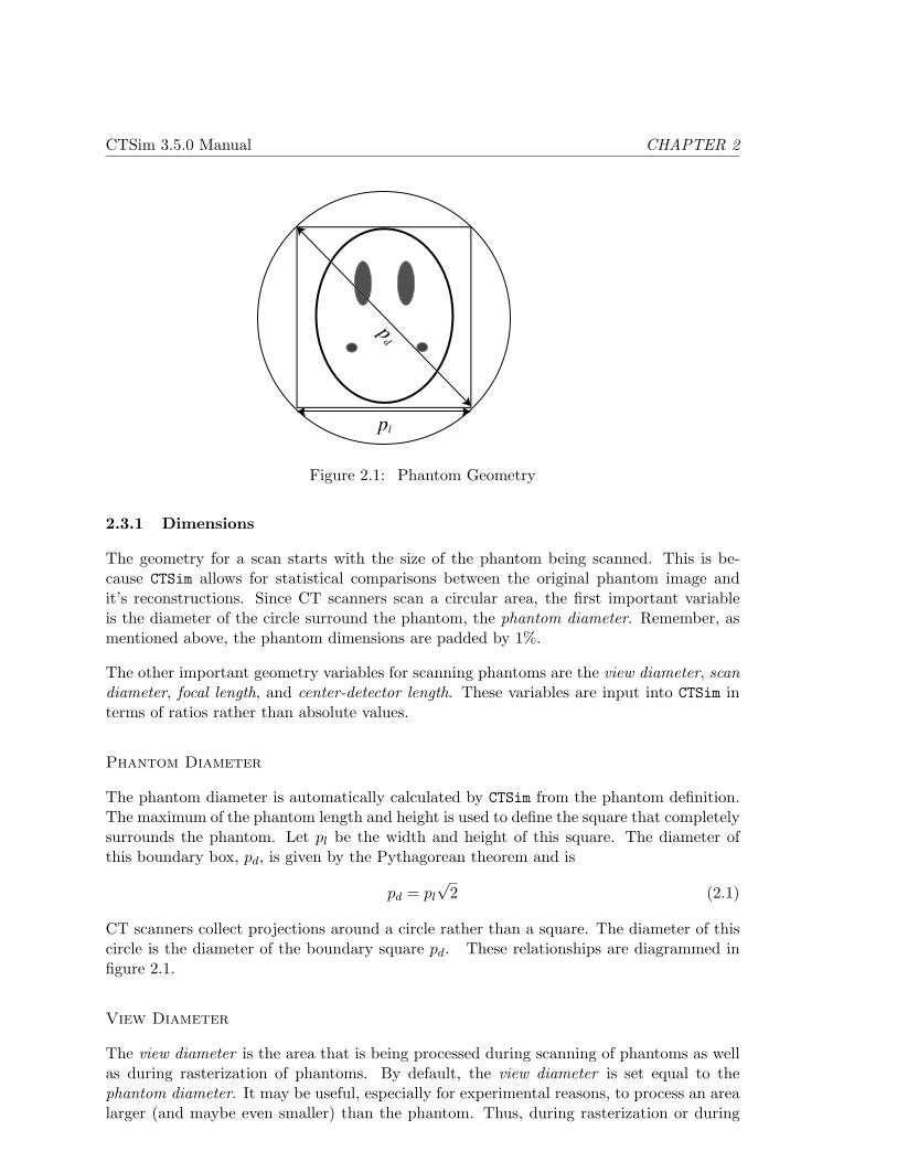
Figure 2.1: Phantom Geometry
2.3.1 Dimensions
The geometry for a scan starts with the size of the phantom being scanned. This is be-cause CTSim allows for statistical comparisons between the original phantom image andit’s reconstructions. Since CT scanners scan a circular area, the first important variableis the diameter of the circle surround the phantom, the phantom diameter. Remember, asmentioned above, the phantom dimensions are padded by 1%.
The other important geometry variables for scanning phantoms are the view diameter, scandiameter, focal length, and center-detector length. These variables are input into CTSim interms of ratios rather than absolute values.
Phantom Diameter
The phantom diameter is automatically calculated by CTSim from the phantom definition.The maximum of the phantom length and height is used to define the square that completelysurrounds the phantom. Let pl be the width and height of this square. The diameter ofthis boundary box, pd, is given by the Pythagorean theorem and is
pd = pl
√2 (2.1)
CT scanners collect projections around a circle rather than a square. The diameter of thiscircle is the diameter of the boundary square pd. These relationships are diagrammed infigure 2.1.
View Diameter
The view diameter is the area that is being processed during scanning of phantoms as wellas during rasterization of phantoms. By default, the view diameter is set equal to thephantom diameter. It may be useful, especially for experimental reasons, to process an arealarger (and maybe even smaller) than the phantom. Thus, during rasterization or during
Manual v1.0 May 1, 2002 4

CTSim 3.5.0 Manual CHAPTER 2
projections, CTSim will ask for a view ratio, vr. The view diameter is then calculated as
vd = pdvr (2.2)
By using a vr less than 1, CTSim will allow for a view diameter less than phantom diameter.This will lead to significant artifacts. Physically, this would be impossible and is analogousto inserting an object into the CT scanner that is larger than the scanner itself!
Scan Diameter
By default, the entire view diameter is scanned. For experimental purposes, it may bedesirable to scan an area either larger or smaller than the view diameter. Thus, the conceptof scan ratio, sr, arises. The scan diameter, sd, is the diameter over which x-rays arecollected and is defined as
sd = vdsr (2.3)
By default and for all ordinary scanning, the scan ratio is to 1. If the scan ratio is less than1, you can expect significant artifacts.
Focal Length
The focal length, f , is the distance of the X-ray source to the center of the phantom. Thefocal length is set as a ratio, fr, of the view radius. Focal length is calculated as
f = (vd/2)fr (2.4)
For parallel geometry scanning, the focal length doesn’t matter. However, for divergentgeometry scanning (equilinear and equiangular), the focal length ratio should be set at 2or more to avoid artifacts. Moreover, a value of less than 1 is physically impossible and itanalagous to having the x-ray source inside of the view diameter.
Center-Detector Length
The center-detector length, c, is the distance from the center of the phantom to the centerof the detector array. The center-detector length is set as a ratio, cr, of the view radius.The center-detector length is calculated as
f = (vd/2)cr (2.5)
For parallel geometry scanning, the center-detector length doesn’t matter. A value of lessthan 1 is physically impossible and it analagous to having the detector array inside of theview diameter.
2.3.2 Parallel Geometry
The simplest geometry, parallel, was used in first generation scanners. As mentioned above,the focal length is not used in this simple geometry. The detector array is set to be the
Manual v1.0 May 1, 2002 5
CTSim 3.5.0 Manual CHAPTER 2
Equilinear Geometry
Det
ecto
rs
Sour
ce
Det
ecto
rs
Sour
ce
Equiangular Geometry
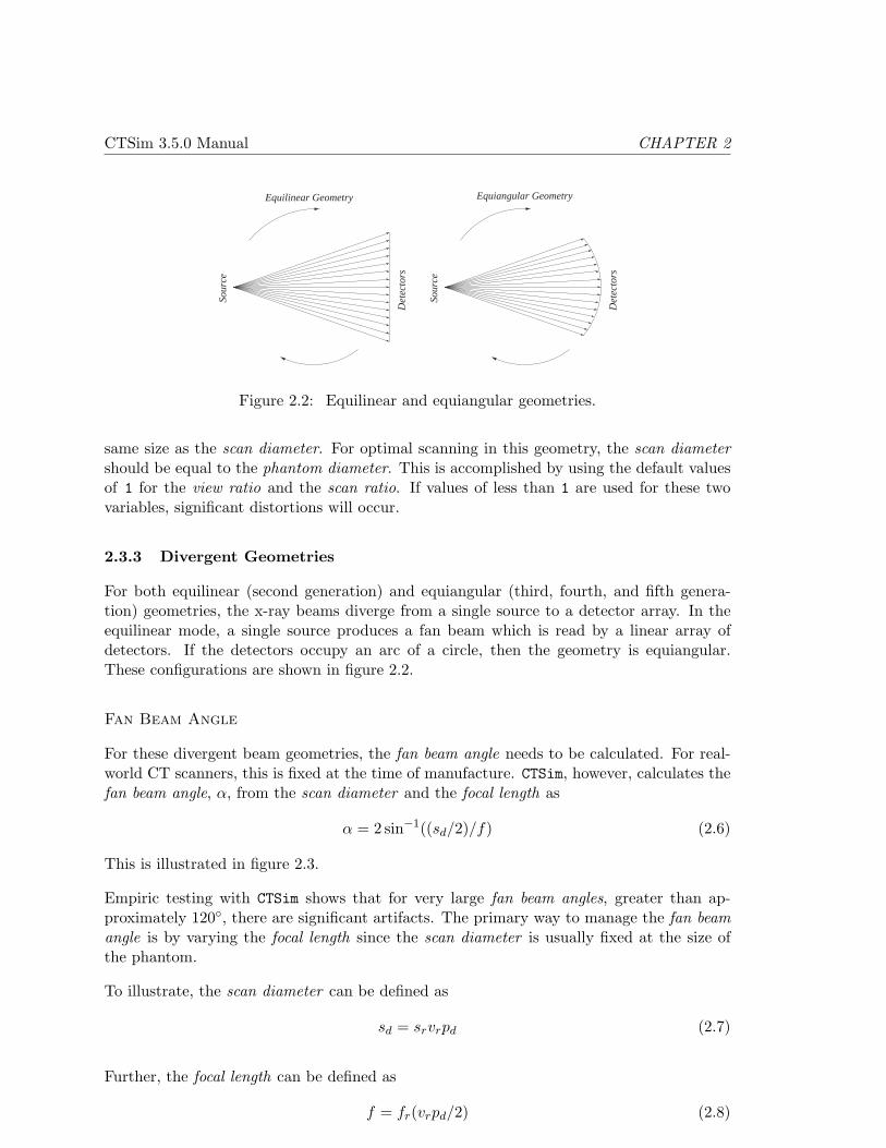
Figure 2.2: Equilinear and equiangular geometries.
same size as the scan diameter. For optimal scanning in this geometry, the scan diametershould be equal to the phantom diameter. This is accomplished by using the default valuesof 1 for the view ratio and the scan ratio. If values of less than 1 are used for these twovariables, significant distortions will occur.
2.3.3 Divergent Geometries
For both equilinear (second generation) and equiangular (third, fourth, and fifth genera-tion) geometries, the x-ray beams diverge from a single source to a detector array. In theequilinear mode, a single source produces a fan beam which is read by a linear array ofdetectors. If the detectors occupy an arc of a circle, then the geometry is equiangular.These configurations are shown in figure 2.2.
Fan Beam Angle
For these divergent beam geometries, the fan beam angle needs to be calculated. For real-world CT scanners, this is fixed at the time of manufacture. CTSim, however, calculates thefan beam angle, α, from the scan diameter and the focal length as
α = 2 sin−1((sd/2)/f) (2.6)
This is illustrated in figure 2.3.
Empiric testing with CTSim shows that for very large fan beam angles, greater than ap-proximately 120◦, there are significant artifacts. The primary way to manage the fan beamangle is by varying the focal length since the scan diameter is usually fixed at the size ofthe phantom.
To illustrate, the scan diameter can be defined as
sd = srvrpd (2.7)
Further, the focal length can be defined as
f = fr(vrpd/2) (2.8)
Manual v1.0 May 1, 2002 6

CTSim 3.5.0 Manual CHAPTER 2
Figure 2.3: Calculation of α
Substituting these equations into equation 2.6, We have,
α = 2 sin−1 srvrpd/2frvr(pd/2)
= 2 sin−1(sr/fr) (2.9)
Since in normal scanning sr = 1, α depends only upon the focal length ratio in normalscanning.
Detector Array Size
In general, you do not need to be concerned with the detector array size – it is automaticallycalculated by CTSim. For the particularly interested, this section explains how the detectorarray size is calculated.
For parallel geometry, the detector length is simply the scan diameter.
For divergent beam geometries, the size of the detector array also depends upon the focallength: increasing the focal length decreases the size of the detector array.
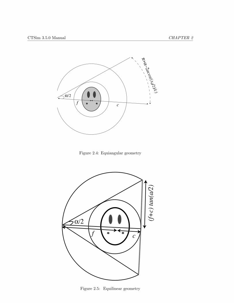
For equiangular geometry, the detectors are equally spaced around a arc covering an angulardistance of α as viewed from the source. When viewed from the center of the scanning, theangular distance is
π + α− 2 cos−1(sd/2
c
)
The dotted circle in figure 2.4 indicates the positions of the detectors in this case.
For equilinear geometry, the detectors are equally spaced along a straight line. The detectorlength depends upon α and the focal length. This length, dl, is calculated as
dl = 2 (f + c) tan(α/2) (2.10)
This geometry is shown in figure 2.5.
Manual v1.0 May 1, 2002 7
CTSim 3.5.0 Manual CHAPTER 2
α/2
π+
α−
2aco
s((sd /2)/c)
f c
Figure 2.4: Equiangular geometry
Figure 2.5: Equilinear geometry
Manual v1.0 May 1, 2002 8
CTSim 3.5.0 Manual CHAPTER 2
2.4 Reconstruction
2.4.1 Direct Inverse Fourier
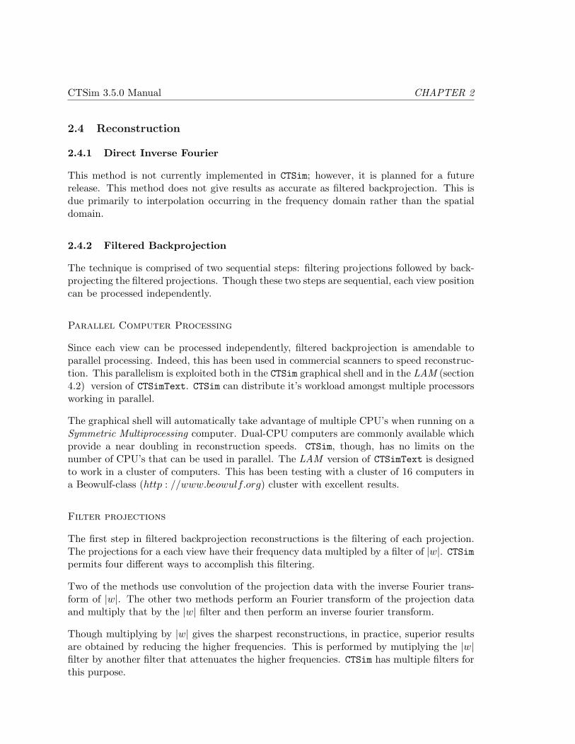
This method is not currently implemented in CTSim; however, it is planned for a futurerelease. This method does not give results as accurate as filtered backprojection. This isdue primarily to interpolation occurring in the frequency domain rather than the spatialdomain.
2.4.2 Filtered Backprojection
The technique is comprised of two sequential steps: filtering projections followed by back-projecting the filtered projections. Though these two steps are sequential, each view positioncan be processed independently.
Parallel Computer Processing
Since each view can be processed independently, filtered backprojection is amendable toparallel processing. Indeed, this has been used in commercial scanners to speed reconstruc-tion. This parallelism is exploited both in the CTSim graphical shell and in the LAM (section4.2) version of CTSimText. CTSim can distribute it’s workload amongst multiple processorsworking in parallel.
The graphical shell will automatically take advantage of multiple CPU’s when running on aSymmetric Multiprocessing computer. Dual-CPU computers are commonly available whichprovide a near doubling in reconstruction speeds. CTSim, though, has no limits on thenumber of CPU’s that can be used in parallel. The LAM version of CTSimText is designedto work in a cluster of computers. This has been testing with a cluster of 16 computers ina Beowulf-class (http : //www.beowulf.org) cluster with excellent results.
Filter projections
The first step in filtered backprojection reconstructions is the filtering of each projection.The projections for a each view have their frequency data multipled by a filter of |w|. CTSimpermits four different ways to accomplish this filtering.
Two of the methods use convolution of the projection data with the inverse Fourier trans-form of |w|. The other two methods perform an Fourier transform of the projection dataand multiply that by the |w| filter and then perform an inverse fourier transform.
Though multiplying by |w| gives the sharpest reconstructions, in practice, superior resultsare obtained by reducing the higher frequencies. This is performed by mutiplying the |w|filter by another filter that attenuates the higher frequencies. CTSim has multiple filters forthis purpose.
Manual v1.0 May 1, 2002 9
CTSim 3.5.0 Manual CHAPTER 2
Backprojection of filtered projections
Backprojection is the process of “smearing” the filtered projections over the reconstructingimage. Various levels of interpolation can be specified.
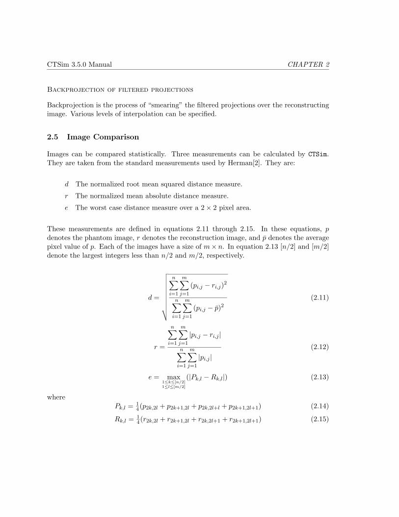
2.5 Image Comparison
Images can be compared statistically. Three measurements can be calculated by CTSim.They are taken from the standard measurements used by Herman[2]. They are:
d The normalized root mean squared distance measure.
r The normalized mean absolute distance measure.
e The worst case distance measure over a 2× 2 pixel area.
These measurements are defined in equations 2.11 through 2.15. In these equations, pdenotes the phantom image, r denotes the reconstruction image, and p̄ denotes the averagepixel value of p. Each of the images have a size of m× n. In equation 2.13 [n/2] and [m/2]denote the largest integers less than n/2 and m/2, respectively.
d =
√√√√√√√√√√
n∑
i=1
m∑
j=1
(pi,j − ri,j)2
n∑
i=1
m∑
j=1
(pi,j − p̄)2(2.11)
r =
n∑
i=1
m∑
j=1
|pi,j − ri,j |n∑
i=1
m∑
j=1
|pi,j |(2.12)
e = max1≤k≤[n/2]1≤l≤[m/2]
(|Pk,l −Rk,l|) (2.13)
wherePk,l = 1
4(p2k,2l + p2k+1,2l + p2k,2l+l + p2k+1,2l+1) (2.14)
Rk,l = 14(r2k,2l + r2k+1,2l + r2k,2l+1 + r2k+1,2l+1) (2.15)
Manual v1.0 May 1, 2002 10

3. The Graphical User Interface
CTSim is the graphical shell for the CTSim project. This shell uses the wxWindows(http : //www.wxwindows.org) library for cross-platform compatibility. The graphicalshell is compatible with Microsoft Windows, GTK (http : //www.gtk.org), and Motif(http : //www.openmotif.org) graphical environments.
3.1 Starting CTSim
Usage
ctsim [files to open...]
You can invoke CTSim by itself on the command line, or include any number of files that youwant CTSim to automatically open. CTSim can open projection files, image files, phantomfiles, and plot files.
On Microsoft Windows platforms, the simplest way to invoke CTSim is via the Start menuunder the Programs sub-menu.
3.2 Quick Start
The fastest way to put CTSim through it’s basic operation is:
1. File - Create Phantom...This creates a window with the geometric phantom. Choose the Herman head phan-tom.
2. Process - Rasterize...This creates an image file of the phantom by converting it from a geometric definitioninto a rasterized image. You may use the defaults shown in the dialog box.
3. View - Auto...Use this command on the new rasterized image window. This will optimize the inten-sity scale for viewing the soft-tissue details of the phantom. Select the median centerand a standard deviation factor of 0.1.
4. Process - Projections...Use this command on the geometric phantom window. This simulates the collectionof x-ray data. You may use the defaults shown in the dialog box. Additionally, youmay wish to turn on Trace - Projections to watch to x-ray data being simulated.
Manual v1.0 May 1, 2002 11
CTSim 3.5.0 Manual CHAPTER 3
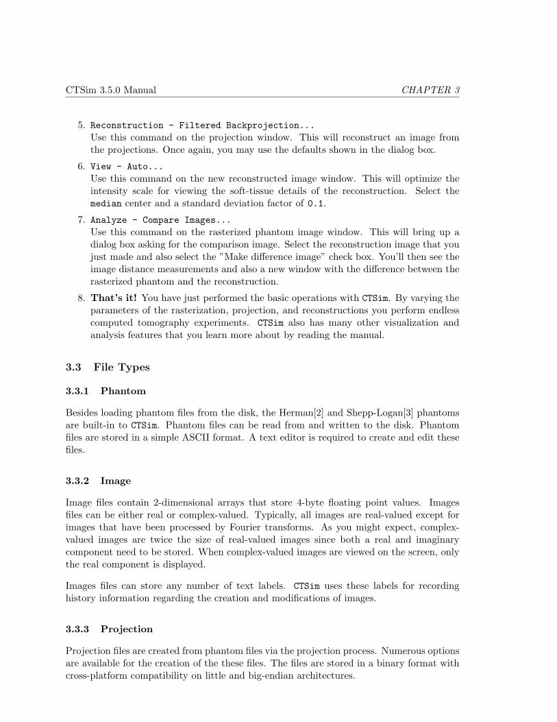
5. Reconstruction - Filtered Backprojection...Use this command on the projection window. This will reconstruct an image fromthe projections. Once again, you may use the defaults shown in the dialog box.
6. View - Auto...Use this command on the new reconstructed image window. This will optimize theintensity scale for viewing the soft-tissue details of the reconstruction. Select themedian center and a standard deviation factor of 0.1.
7. Analyze - Compare Images...Use this command on the rasterized phantom image window. This will bring up adialog box asking for the comparison image. Select the reconstruction image that youjust made and also select the ”Make difference image” check box. You’ll then see theimage distance measurements and also a new window with the difference between therasterized phantom and the reconstruction.
8. That’s it! You have just performed the basic operations with CTSim. By varying theparameters of the rasterization, projection, and reconstructions you perform endlesscomputed tomography experiments. CTSim also has many other visualization andanalysis features that you learn more about by reading the manual.
3.3 File Types
3.3.1 Phantom
Besides loading phantom files from the disk, the Herman[2] and Shepp-Logan[3] phantomsare built-in to CTSim. Phantom files can be read from and written to the disk. Phantomfiles are stored in a simple ASCII format. A text editor is required to create and edit thesefiles.
3.3.2 Image
Image files contain 2-dimensional arrays that store 4-byte floating point values. Imagesfiles can be either real or complex-valued. Typically, all images are real-valued except forimages that have been processed by Fourier transforms. As you might expect, complex-valued images are twice the size of real-valued images since both a real and imaginarycomponent need to be stored. When complex-valued images are viewed on the screen, onlythe real component is displayed.
Images files can store any number of text labels. CTSim uses these labels for recordinghistory information regarding the creation and modifications of images.
3.3.3 Projection
Projection files are created from phantom files via the projection process. Numerous optionsare available for the creation of the these files. The files are stored in a binary format withcross-platform compatibility on little and big-endian architectures.
Manual v1.0 May 1, 2002 12
CTSim 3.5.0 Manual CHAPTER 3
3.3.4 Plot
Plot files are created by CTSim during analysis of image files. They can be read from andwritten to the disk. They are stored as ASCII files for easy cross-platform support andediting.
3.4 Global Menu Commands
These global commands are present on the menus of all windows.
3.4.1 File - Create Phantom
This command displays a dialog box showing the phantoms that are pre-programmed intoCTSim. After selecting one of these phantoms, the new window with that phantom will begenerated. The pre-programmed phantoms are:
Herman The Herman head phantom[2]
Shepp-Logan The head phantom of Shepp & Logan[3]
Unit pulse A phantom that has a value of 1 for the center ofthe phantom and 0 everywhere else.
3.4.2 File - Create Filter
This command displays a dialog box showing the pre-programmed filters of CTSim. Thiscommand will create a 2-dimensional image of the selected filter. The center of the filter isat the center of the image.
These filters can be created in their natural frequency domain or in their inverse spatialdomain.
Manual v1.0 May 1, 2002 13

CTSim 3.5.0 Manual CHAPTER 3
Filter Selects the filter to generate. The available filtersare:
• |w| Bandlimit
• |w| Hamming
• |w| Hanning
• |w| Cosine
• |w| Sinc
• Shepp
• Bandlimit
• Sinc
• Hamming
• Hanning
• Cosine
• Triangle
Domain Selects either the Frequency or Spatial domain.The filters have the frequency domain as their nat-ural domain. The spatial domain is obtained eitheranalytically or performing an inverse Fourier trans-formation.
X Size Number of columns in the output image.
Y Size Number of rows in the output image.
Hamming Parameter This parameter adjusts the smoothing of the Ham-ming filter and can range from 0 to 1. At a settingof 1, the Hamming filter is the same as the ban-dlimit filter. At a setting of 0.54, the Hammingfilter is the same as the Hanning window.
Bandwidth Sets the bandwidth of the filter.
Manual v1.0 May 1, 2002 14
CTSim 3.5.0 Manual CHAPTER 3
Axis (input) Scale Sets the scale for the filter input. By default, theinput to the filter is the distance in pixels from thecenter of the image. By changing this value, onecan set a scale the input to the filter. For example,if the output image is 101 by 101 pixels and thusthe center of the image is at (50,50), then a pixellying at point 100,50 would be 50 units from thecenter of the filter. By applying an Axis scaleof 0.1, then that point would be scaled to 5 unitsfrom the center of the filter.
Filter (output) Scale Multiplies the output of the filter by this amount.By default, the filter has a maximum value of 1.
3.4.3 File - Import
This command allows the importing of non-CTSim file formats into CTSim. PPM and PNGformats will be read into an imagefile window. Color images will be converted to grayscale.If a DICOM library was linked in with your version of CTSim, then you can also import DICOMprojection files and image files.
3.4.4 File - Preferences
This command displays a dialog box that allows users to control the behavior of CTSim.These options are saved across CTSim sessions. Under Microsoft Windows environments,they are stored in the registry. On UNIX and Linux environments, they are stored in theuser’s home directory with the filename of .ctsim.
Manual v1.0 May 1, 2002 15
CTSim 3.5.0 Manual CHAPTER 3
Advanced options This option is initially turned off in new installa-tions. These advanced options are not required fornormal simulations. When Advanced Options isset, CTSim will display more options during scan-ning of phantoms and the reconstruction of projec-tions.
Ask before closing new documents This option is initially turned on in new installa-tions. With this option set, CTSim will ask beforeclosing documents that have been modified or neversaved on disk. By turning off this option, CTSimwill never ask if you want to save a file – you’ll beresponsible for saving any files that you create.
Verbose logging This option is initially turned off in new installa-tions. With this option set, CTSim will log moreevents than usual. There extra events are notimportant for viewing with typical operation ofCTSim.
Show startup tips This option is initially turned on in new installa-tions. With this option set, CTSim will display help-ful tips when CTSim is started.
Run background tasks This option is initially turned off in new installa-tions. With this option set, CTSim execute lengthycalculations in the background. A background win-dow will appear when processes are running inthe background and will disappear when no back-ground processes are executing. This backgroundwindow shows the status and progress of all back-ground processes. NOTE: Due to limitations ofwxWindows, this function is only supported on Mi-crosoft Windows.
3.4.5 File - Open
This command opens a file section dialog box. Of special consideration is the File Typecombo box on the bottom of the dialog. You need to set the this combo box to the type offile that you wish to open.
3.4.6 File - Save
This command saves the contents of the active window. If the window hasn’t been named,a dialog box will open asking for the file name to use.
Manual v1.0 May 1, 2002 16
CTSim 3.5.0 Manual CHAPTER 3
3.4.7 File - Close
As one would expect, this closes the active window. If the contents of the window have notbeen saved and the Advanced Preferences option Ask before closing new documents isturned on, then you will be prompted if decide if you want to save the contents of thewindow prior to closing.
3.4.8 File - Save As
Allows the saving of the contents of the active window to any file name.
3.4.9 Help - Contents
This command displays the online help.
3.4.10 Help - Tips
This command displays a dialog with tips on using CTSim.
3.4.11 Help - Quick Start
This command displays a recommend approach to helping new users learn to use CTSim.
3.4.12 Help - About
This command shows the version number and operating environment of CTSim.
3.5 Phantom Menus
3.5.1 Properties
Displays the properties of a phantom which includes:
• Overall dimensions of a phantom
• A list of all component phantom elements
3.5.2 Process - Rasterize
This creates an image file from a phantom. Technically, it converts the phantom from avector (infinite resolution) object into a 2-dimension array of floating-point pixels. Theparameters to set are:
Manual v1.0 May 1, 2002 17
CTSim 3.5.0 Manual CHAPTER 3
X size Number of columns in image file
Y size Number of rows in image file
Samples per pixel Numbers of samples taken per pixel in both the xand y directions. For example, if the Samples perpixel is set to 3, then for every pixel in the imagefile 9 samples (3× 3) are averaged.
3.5.3 Process - Projections
This command creates a projection file from a phantom. The options available when col-lecting projections are:
Geometry Sets the scanner geometry. The available geome-tries are:
• Parallel
• Equiangular
• Equilinear
Number of detectors Sets the number of detectors in the detector array.
Number of views Sets the number of views to collect.
Samples per detector Sets the number of samples collected for each de-tector.
View Ratio Sets the field of view as a ratio of the diameter ofthe phantom. For normal scanning, use a value of1.0.
Scan Ratio Sets the length of scanning as a ratio of the viewdiameter. For normal scanning, use a value of 1.0.
Focal length ratio Sets the distance between the radiation source andthe center of the phantom as a ratio of the radiusof the phantom. For parallel geometries, a value of1.0 is optimal. For other geometries, this shouldbe at least 2.0 to avoid artifacts.
Advanced Options
These options are visible only if Advanced Options has been selected in the File - Preferencesdialog. These parameters default to optimal settings and don’t need to be adjusted except
Manual v1.0 May 1, 2002 18
CTSim 3.5.0 Manual CHAPTER 3
by expert users.
Rotation Angle Sets the rotation amount as a fraction of a circle.For parallel geometries use a rotation angle of 0.5and for equilinear and equiangular geometries use arotation angle of 1. Using any other rotation anglewill lead to artifacts.
3.6 Image Menus
3.6.1 File - Properties
Properties of image files include:
• Whether the image is real or complex-valued.
• Numeric statistics (minimum, maximum, mean, median, mode, and standard devia-tion).
• History labels (text descriptions of the processing for this image).
3.6.2 File - Export
This command allows for exporting image files to a standard graphics file format. This ishelpful when you want to take an image and import it into another application. The currentintensity scale is used when exporting the file. The supported graphic formats are:
PNG Portable Network Graphics format. This uses 8-bits or 256 shades of gray.
PNG-16 This is a 16-bit version of PNG which allows for65536 shades of gray.
PGM Portable Graymap format. This is a common for-mat used on UNIX systems.
PGM ASCII ASCII version of PGM.
3.6.3 View
Intensity Scale
These commands are used change the intensity scale for viewing the image. These com-mands do not change the image data. When the minimum value is set, then the color pureblack is assigned to that image value. Similarly, when the maximum value is set, the thecolor pure white is assigned to that image value.
Manual v1.0 May 1, 2002 19
CTSim 3.5.0 Manual CHAPTER 3
Changing the intensity scale is useful when examining different image features. In clinicalmedicine, the intensity scale is often changed to examine bone (high value) versus soft-tissue(medium value) features.
Set
This command displays a dialog box that sets the lower and upper values to display.
Auto
This command displays a dialog box that allows CTSim to automatically make an intensityscale. The parameters that CTSim needs to make this automatic scale are:
Center This sets the center of the intensity scale. Cur-rently, CTSim allows you to use either the mean,mode, or median of the image as the center of theintensity scale.
Width This sets the half-width of the intensity scale. Thehalf-width is specified as a multiple of the standarddeviation.
As an example, if median is selected as the center and 0.5 is selected as the width, the theminimum value will be median− 0.5× standardDeviation and the maximum value will bemedian + 0.5× standardDeviation.
Full
This command resets the intensity scale to the full scale of the image.
3.6.4 Image
These commands create a new image based upon the current image, and for some commands,also upon a comparison image.
Add, Subtract, Multiply, Divide
These are simple arithmetic operations. CTSim will display a dialog box showing all of thecurrently opened image files that are the same size as the active image. After the selectionof a compatible image, CTSim will perform the arithmetic operation on the two images andmake a new result image.
Image Size
This command will generate a new image based on the current image. The new imagecan be scaled to any size. A dialog appears asking for the size of the new image. Bilinear
Manual v1.0 May 1, 2002 20
CTSim 3.5.0 Manual CHAPTER 3
interpolation is used when calculating the new image.
3-D Conversion
This command generates a 3-dimensional view of the current phantom. This view can berotated in three dimensions. The left and right arrow control the z-axis rotation and theup and down arrows control the x-axis rotation. The y-axis rotation is controlled by the Tand Y keys. Other options are presented on the View menu and include:
• Surface plot versus wireframe plot.
• Smooth shading versus flat shading.
• Lighting on or off.
• Color scale on or off.
3.6.5 Filter
These commands filter and modify the image
Arithmetic
These commands operate on the image on a pixel-by-pixel basis. The commands supportboth real and complex-valued images. The available arithmetic commards are:
Invert Negate pixel values.
Log Take natural logrithm of pixel values.
Exp Take natural exponent of pixel values.
Square Take square of pixel values.
Square root Take square root of pixel values.
Frequency Based
These commands perform Fourier and inverse Fourier transformations of images. By default,the transformations will automatically convert images between Fourier to natural orders asexpected. For example, 2-D FFT will transform the points into natural order after theFourier transform. Similarly the inverse, 2-D IFFT, will reorder the points from naturalorder to Fourier order before applying the inverse Fourier transformation.
As you would expect, images that undergo frequency filtering will be complex-valued afterthan filtering. Only the real component is shown by CTSim. However, CTSim does haveoptions for converting a complex-valued image into a real-valued image via the Magnitudeand Phase filtering commands.
Manual v1.0 May 1, 2002 21
CTSim 3.5.0 Manual CHAPTER 3
The available frequency-based filtering commards are:
• 2-D FFT
• 2-D IFFT
• FFT Rows
• IFFT Rows
• FFT Columns
• IFFT Columns
• 2-D Fourier
• 2-D Inverse Fourier
• Shuffle Fourier to Natural Order
• Shuffle Natural to Fourier Order
• Magnitude
• Phase
3.6.6 Analyze - Plot
The commands plot rows and columns of images. There are commands that perform FFTtransformations prior to plotting. To select the row or column to plot, click the left mousebutton over the desired cursor point.
The available plot commands are:
• Plot Row
• Plot Column
• Plot Histogram
• Plot FFT Row
• Plot FFT Col
3.6.7 Analyze - Compare
This command performs statistical comparisons between two images. An option also existsfor generating a difference image from the two input images.
The three distance measures reported are:
d The normalized root mean squared distance measure.
r The normalized mean absolute distance measure.
e The worst case distance measure over a 2× 2 pixel area.
Manual v1.0 May 1, 2002 22
CTSim 3.5.0 Manual CHAPTER 3
There are also commands for comparison plotting of rows and columns from two images.This is quite helpful when comparing a phantom to a reconstruction. As with plotting ofrows and columns, click the left mouse button over the desired cursor point to choose whichrow and column to plot.
3.7 Projection Menus
3.7.1 File - Properties
The displayed properties include:
• Number of detectors in the projections.
• Number of views.
• The parameters used when generating the projections from the phantom.
3.7.2 Process - Convert Rectangular
The commands takes the projection data and creates an image file using the projectiondata.
3.7.3 Process - Convert Polar
This command creates an image file with the polar conversion of the projection data. Theparameters to set are:
X Size Number of columns in output image.
Y Ssize Number of rows in output image.
Interpolation Selects the interpolation method. Currently, thebilinear option provides the highest quality in-terpolation.
3.7.4 Convert - Convert FFT Polar
The parameters for this option are the same as the Convert Polar Dialog. For this command,though, the projections are Fourier transformed prior to conversion to polar image.
3.7.5 Convert - Interpolate to Parallel
This command filters divergent projection data (equiangular or equilinear) and interpolates(or rebins) to estimate the projection data if the projections had been collected with parallelgeometry.
Manual v1.0 May 1, 2002 23
CTSim 3.5.0 Manual CHAPTER 3
3.7.6 Analyze - Plot Histogram
Plots a histogram of projection data attenuations.
3.7.7 Analyze - Plot T-Theta Sampling
Plots a 2-dimensional scattergram showing the T and Theta values for each data point inthe projection data. This is especially instructive when scanning with divergent geometriesand the scan ratio is close to 1.
Theta Range
This dialog box allows the constraint of Theta values for the T-Theta Sampling scattergram.
3.7.8 Reconstruct - Filtered Backprojection
This command displays a dialog to set the parameters for reconstructing an image fromprojections using the filtered backprojection technique. The parameters available are:
Manual v1.0 May 1, 2002 24
CTSim 3.5.0 Manual CHAPTER 3
Filter Selects the filter to apply to each projection. Toproperly reconstruct an image, this filter shouldconsist of the the absolute value of distance fromzero frequency optionally multiplied by a smooth-ing filter. The optimal filters to use are:
• abs bandlimit
• abs hamming
• abs hanning
• abs cosine
Hamming parameter Sets the alpha level for Hamming window. Thisparameter adjusts the smoothing of the Hammingfilter and can range from 0 to 1. At a setting of1, the Hamming filter is the same as the bandlimitfilter. At a setting of 0.54, the Hamming filter isthe same as the Hanning window.
Filter Method Selects the filtering method. For large num-bers of detectors, the FFT-based filters are pre-ferred whereas for smaller numbers of detectorsconvolution can be faster. When Advanced Op-tions have been turned off, this menu only showsthe two basic choices: convolution and FFT. How-ever, when Advanced Options have been turned on,additional selections are available as discussed inthe next section.
Interpolation Interpolation technique during backprojection.cubic has optimal quality when the data is smooth.Smooth data is obtained by taking many projec-tions and/or using a smoothing filter. In the ab-sence of smooth data, linear gives better resultsand is also many times faster than cubic interpola-tion.
• nearest - No interpolation, selects nearestpoint.
• linear - Uses fast straight line interpolation.
• cubic - Uses cubic interpolating polynomial.
Advanced Options
These options are visible only if Advanced Options has been selected in the File - Preferences
Manual v1.0 May 1, 2002 25

CTSim 3.5.0 Manual CHAPTER 3
dialog. These parameters default to optimal settings and don’t need to be adjusted exceptby expert users.
Manual v1.0 May 1, 2002 26
CTSim 3.5.0 Manual CHAPTER 3
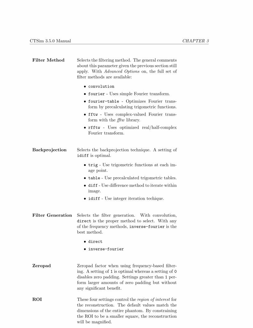
Filter Method Selects the filtering method. The general commentsabout this parameter given the previous section stillapply. With Advanced Options on, the full set offilter methods are available:
• convolution
• fourier - Uses simple Fourier transform.
• fourier-table - Optimizes Fourier trans-form by precalculating trigometric functions.
• fftw - Uses complex-valued Fourier trans-form with the fftw library.
• rfftw - Uses optimized real/half-complexFourier transform.
Backprojection Selects the backprojection technique. A setting ofidiff is optimal.
• trig - Use trigometric functions at each im-age point.
• table - Use precalculated trigometric tables.
• diff - Use difference method to iterate withinimage.
• idiff - Use integer iteration techique.
Filter Generation Selects the filter generation. With convolution,direct is the proper method to select. With anyof the frequency methods, inverse-fourier is thebest method.
• direct
• inverse-fourier
Zeropad Zeropad factor when using frequency-based filter-ing. A setting of 1 is optimal whereas a setting of 0disables zero padding. Settings greater than 1 per-form larger amounts of zero padding but withoutany significant benefit.
ROI These four settings control the region of interest forthe reconstruction. The default values match thedimensions of the entire phantom. By constrainingthe ROI to be a smaller square, the reconstructionwill be magnified.
Manual v1.0 May 1, 2002 27

CTSim 3.5.0 Manual CHAPTER 3
3.7.9 Reconstruct - Filtered Backprojection (Rebin to Parallel)
The command reconstructs the projection data via filtered backprojection as describedabove. As opposed to the above command, this command also rebins divergent projectiondata to parallel prior to reconstruction. This greatly speeds reconstruction of divergentgeometry projections.
3.8 Plot Menus
3.8.1 File - Properties
The displayed properties include:
• the number of curves in the plot and the number of points per curve.
• the EZPlot commands used to format the plot are displayed.
• history labels from the originating image(s) and the plot function.
3.8.2 View Menu
These commands set the scaling for the y-axis. They are analogous to the options used forsetting the intensity scale for images.
Set
This command sets the upper and lower limits for the y-axis.
Auto
This command automatically sets the upper and lower limits for the y-axis. Please refer tothe image file View - Auto (section 3.6.3) documentation for the details.
Full
The command resets the upper and lower limits of the y-axis to the minimum and maximumvalues of the curves.
Manual v1.0 May 1, 2002 28
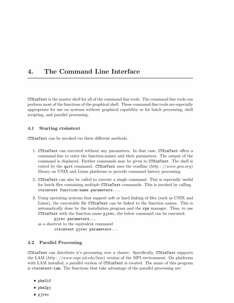
4. The Command Line Interface
CTSimText is the master shell for all of the command-line tools. The command-line tools canperform most of the functions of the graphical shell. These command-line tools are especiallyappropriate for use on systems without graphical capability or for batch processing, shellscripting, and parallel processing.
4.1 Starting ctsimtext
CTSimText can be invoked via three different methods.
1. CTSimText can executed without any parameters. In that case, CTSimText offers acommand-line to enter the function-names and their parameters. The output of thecommand is displayed. Further commands may be given to CTSimText. The shell isexited by the quit command. CTSimText uses the readline (http : //www.gnu.org)library on UNIX and Linux platforms to provide command history processing.
2. CTSimText can also be called to execute a single command. This is especially usefulfor batch files containing multiple CTSimText commands. This is invoked by callingctsimtext function-name parameters....
3. Using operating systems that support soft or hard linking of files (such as UNIX andLinux), the executable file CTSimText can be linked to the function names. This isautomatically done by the installation program and the rpm manager. Thus, to useCTSimText with the function name pjrec, the below command can be executed:
pjrec parameters...as a shortcut to the equivalent command
ctsimtext pjrec parameters...
4.2 Parallel Processing
CTSimText can distribute it’s processing over a cluster. Specifically, CTSimText supportsthe LAM (http : //www.mpi.nd.edu/lam) version of the MPI environment. On platformswith LAM installed, a parallel version of CTSimText is created. The name of this programis ctsimtext-lam. The functions that take advantage of the parallel processing are:
• phm2if
• phm2pj
• pjrec
Manual v1.0 May 1, 2002 29
CTSim 3.5.0 Manual CHAPTER 4
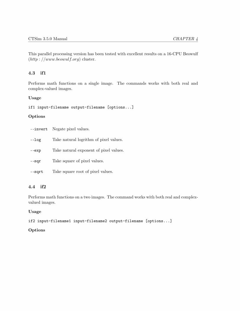
This parallel processing version has been tested with excellent results on a 16-CPU Beowulf(http : //www.beowulf.org) cluster.
4.3 if1
Performs math functions on a single image. The commands works with both real andcomplex-valued images.
Usage
if1 input-filename output-filename [options...]
Options
- -invert Negate pixel values.
- -log Take natural logrithm of pixel values.
- -exp Take natural exponent of pixel values.
- -sqr Take square of pixel values.
- -sqrt Take square root of pixel values.
4.4 if2
Performs math functions on a two images. The command works with both real and complex-valued images.
Usage
if2 input-filename1 input-filename2 output-filename [options...]
Options
Manual v1.0 May 1, 2002 30
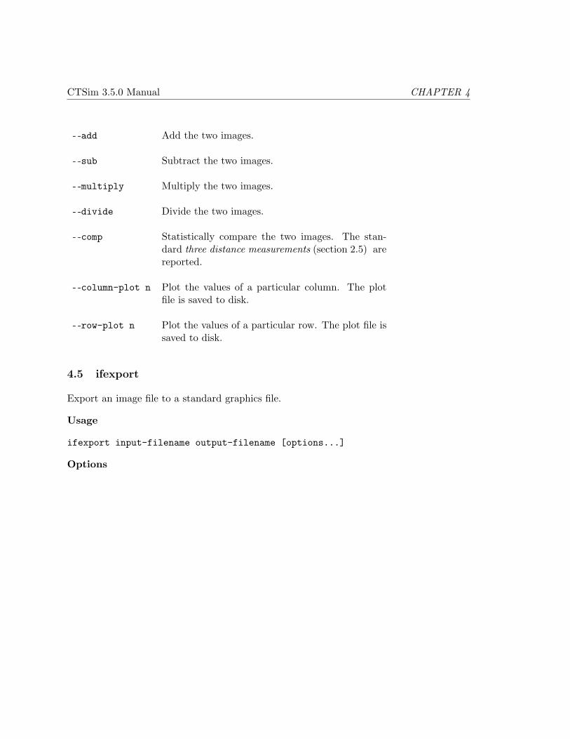
CTSim 3.5.0 Manual CHAPTER 4
- -add Add the two images.
- -sub Subtract the two images.
- -multiply Multiply the two images.
- -divide Divide the two images.
- -comp Statistically compare the two images. The stan-dard three distance measurements (section 2.5) arereported.
- -column-plot n Plot the values of a particular column. The plotfile is saved to disk.
- -row-plot n Plot the values of a particular row. The plot file issaved to disk.
4.5 ifexport
Export an image file to a standard graphics file.
Usage
ifexport input-filename output-filename [options...]
Options
Manual v1.0 May 1, 2002 31

CTSim 3.5.0 Manual CHAPTER 4
- -format• png - Portable network graphics format. This
is the default output format.
• png16 - 16-bit PNG format.
• pgm - Portable graymap format, binary for-mat.
• pgmasc - ASCII PGM format.
- -center Set center of intensity window.
• median
• mode
• mean
- -auto Set half-width of intensity window as a multiple ofthe standard deviation.
• full
• std0.1
• std0.5
• std1
• std2
• std3
- -scale Set size of output image. A value of 1 is defaultand creates an output image the same size as theinput image. A value of 2 will double the size ofthe output image.
- -min Set the minimum intensity value.
- -max Set the maximum intensity value.
4.6 ifinfo
Displays information about an image file. By default, history labels and image statisticsare displayed.
Usage
ifinfo input-filename [options...]
Manual v1.0 May 1, 2002 32
CTSim 3.5.0 Manual CHAPTER 4
Options
- -no-labels Suppress history labels.
- -no-stats Suppress image statistics.
4.7 phm2pj
Simulates collection of X-rays data (projections) around a phantom object.
Usage
phm2pj projection-filename number-detectors number-views [options...]
Options
Manual v1.0 May 1, 2002 33
CTSim 3.5.0 Manual CHAPTER 4
- -phantom Select a standard phantom.
• herman
• shepp-logan
• unit-pulse
- -phmfile Reads a user-created phantom file.
- -geometry Sets the scanner geometry. Valid values are:
• parallel
• equiangular
• equilinear
- -nray Number of samples per each detector
- -rotangle The rotation angle as a fraction of a circle. For par-allel geometries use a rotation angle of 0.5 and forequilinear and equiangular geometries use a rota-tion angle of 1. The default is to use to appropriaterotation angle based on the geometry.
- -view-ratio Sets the field of view as a ratio of the diameterof the phantom. For normal scanning, the defaultvalue of 1.0 is optimal.
- -scan-ratio Sets the length of scanning as a ratio of the viewdiameter. For normal scanning, the default valueof 1.0 is optimal.
- -focal-length Sets the distance between the radiation source andthe center of the object as a ratio of the radius ofthe object. For parallel geometries, a value of 1.0is optimal. For other geometries, this should be atleast 2.0 to avoid artifacts. The default value is 2.
4.8 phm2if
Generates a raster image file based on a phantom.
Usage
phm2if phantom-filename image-filename x-image-size y-image-size [options...]
Manual v1.0 May 1, 2002 34
CTSim 3.5.0 Manual CHAPTER 4
Options
- -nsamples Number of samples in x and y directions per pixel
- -view-ratio Sets the view ratio. For normal scanning, the de-fault value of 1.0 is optimal.
4.9 pj2if
Convert a projection file into an image file where each row of the image file contains theprojection data from a single view.
Usage
pj2if projection-filename image-filename [options...]
Options
- -dump Print all projection data to the console.
4.10 pjinfo
Displays information about a projection file.
Usage
pjinfo projection-filename [options...]
Options
- -binaryheader Dump the binary header to the standard output.This option is only used when manually creatinga composite projection file from several differentprojection files.
- -binaryview Dump binary view data to the standard output.This option is only used when manually creatinga composite projection file from several differentprojection files.
- -startview Sets starting view to display. Default is 0.
- -endview Sets ending view to display. Default is the last view.
- -dump Print all projection data to the console.
Manual v1.0 May 1, 2002 35
CTSim 3.5.0 Manual CHAPTER 4
4.11 pjrec
Reconstructs the interior of an object from a projection file.
Usage
pjrec projection-filename image-filename image-cols image-rows [options...]
Options
Parameter Options
- -filter Selects which filter to apply to each projection. Toproperly reconstruct an image, this filter shouldconsist of the the absolute value of distance fromzero frequency optionally multiplied by a smooth-ing filter. The optimal filters to use are:
• abs bandlimit
• abs cosine
• abs hamming
• abs hanning
- -filter-parameter Sets the alpha level for Hamming window. Thisparameter adjusts the smoothing of the Hammingfilter and can range from 0 to 1. At a setting of1, the Hamming filter is the same as the bandlimitfilter. At a setting of 0.54, the Hamming filter isthe same as the Hanning window.
- -filter-method Selects the filtering method. For large numbers ofdetectors, rfftw is optimal. For smaller numbersof detectors, convolution might be a bit faster.
• convolution
• fourier - Uses simple Fourier transform.
• fourier-table - Optimizes Fourier trans-form by precalculating trigometric functions.
• fftw - Uses complex-valued Fourier trans-form with the fftw library.
• rfftw - Uses optimized real/half-complexFourier transform.
Manual v1.0 May 1, 2002 36

CTSim 3.5.0 Manual CHAPTER 4
- -filter-generation Selects the filter generation. With convolution,direct is the proper method to select. With anyof the frequency methods, inverse-fourier is thebest method.
• direct
• inverse-fourier
- -interpolation Interpolation technique during backprojection.cubic has optimal quality when the data is smooth.Smooth data is obtained by taking many projec-tions and/or using a smoothing filter. In the ab-sence of smooth data, linear gives better resultsand is many times faster than cubic interpolation.
• nearest - No interpolation, selects nearestpoint.
• linear - Uses fast straight line interpolation.
• cubic - Uses cubic interpolating polynomial.
- -backprojection Selects the backprojection technique. A setting ofidiff is optimal.
• trig - Use trigometric functions at each im-age point.
• table - Use precalculated trigometric tables.
• diff - Use difference method to iterate withinimage.
• idiff - Use integer iteration technique.
- -zeropad Zeropad factor. A setting of 1 is optimal whereasa zeropad of 0 performs no zero padding. Settingsgreater than 1 perform additional zero padding, butwithout any significant output difference.
Manual v1.0 May 1, 2002 37

5. The Web Interface
5.1 Overview
CTSim can also be executed via a web browser. The Perl program ctsim.cgi takes pro-jections of a standard phantom object, performs reconstruction, and then compares therasterized phantom object with the reconstruction. The comparison is performed bothvisually by an image subtraction as well as by statistical analysis.
The ctsim.cgi program is invoked from the HTML file simulate.html.
5.2 Requirements
• Apache (http : //www.apache.org) or other CGI-compatible web server
• Perl (version 4.0 or higher)
• A client web browser than can display PNG files. Most current web browsers supportPNG.
• A knowledgable system administrator.
5.3 Installation
Installation is rather automatic on Linux and UNIX systems. The configure script needsto be given options that specify the directory for web pages and for CGI programs.
Manual v1.0 May 1, 2002 38
6. Installation
6.1 Download
The latest version of CTSim, both as executable programs and source code, can be down-loaded from the official CTSim web site (http : //www.ctsim.org). Additionally, these filesare also available from the CTSim FTP site (files : //files.b9.com/ctsim).
6.2 Installing Windows Binary
Download the Windows executable file. Simply execute this program to begin the instal-lation program. CTSim will then be accessible from the Start Menu under the Programssubmenu.
CTSim is compatible with Windows 98, Windows Me, Windows NT 4.0, and Windows 2000.Due to use of the OpenGL and htmlhelp libraries, CTSim is not compatible with the stockWindows 95 system.
6.3 Installing Linux RPM
Download the CTSim RPM file, then use the rpm manager program as follows:rpm -Uvh ctsim-*.rpm
CTSim and CTSimText will then be installed in the /usr/local/bin directory. The onlinehelp file, ctsim.hhp, will be installed in directory /usr/local/man.
6.4 Build From Sources
Refer to the INSTALL file included in the source distribution for instructions.
6.4.1 Optional Libraries
These libraries are optional and not required to build CTSim from source code. However,they add functionality to CTSim and there inclusion is recommended.
• wxWindows 2.3Used for the platform-independent graphical interface. The graphical version of CTSimrequires this library.
Manual v1.0 May 1, 2002 39
CTSim 3.5.0 Manual CHAPTER 6
Web site (http : //www.wxwindows.org)
• FFTW3Used for fast Fourier transformations of projections and images. Without this libraryCTSim will use slower, traditional Fourier transformations.Web site (http : //www.fftw.org)
• libpngUsed for PNG file export.Web site (http : //www.libpng.org/pub/png/libpng.html)
• zlibUsed for PNG file export.Web site (http : //www.info− zip.org/pub/infozip/zlib/zlibdocs.html)
• readlineUsed for CTSimText interactive shell.Web site (http : //www.gnu.org)
• dmallocUsed for debugging memory allocation.Web site (http : //www.dmalloc.com)
• ctnDICOM library used to support import/export of DICOM files Web site (http ://www.erl.wustl.edu/DICOM/ctn.html)
Manual v1.0 May 1, 2002 40
A. Algorithms
CTSim uses a number of interesting algorithms. This appendix details some of the techniquesthat CTSim uses.
A.1 Phantom Processing
Key ConceptsGeometric transformationsMatrix algebra
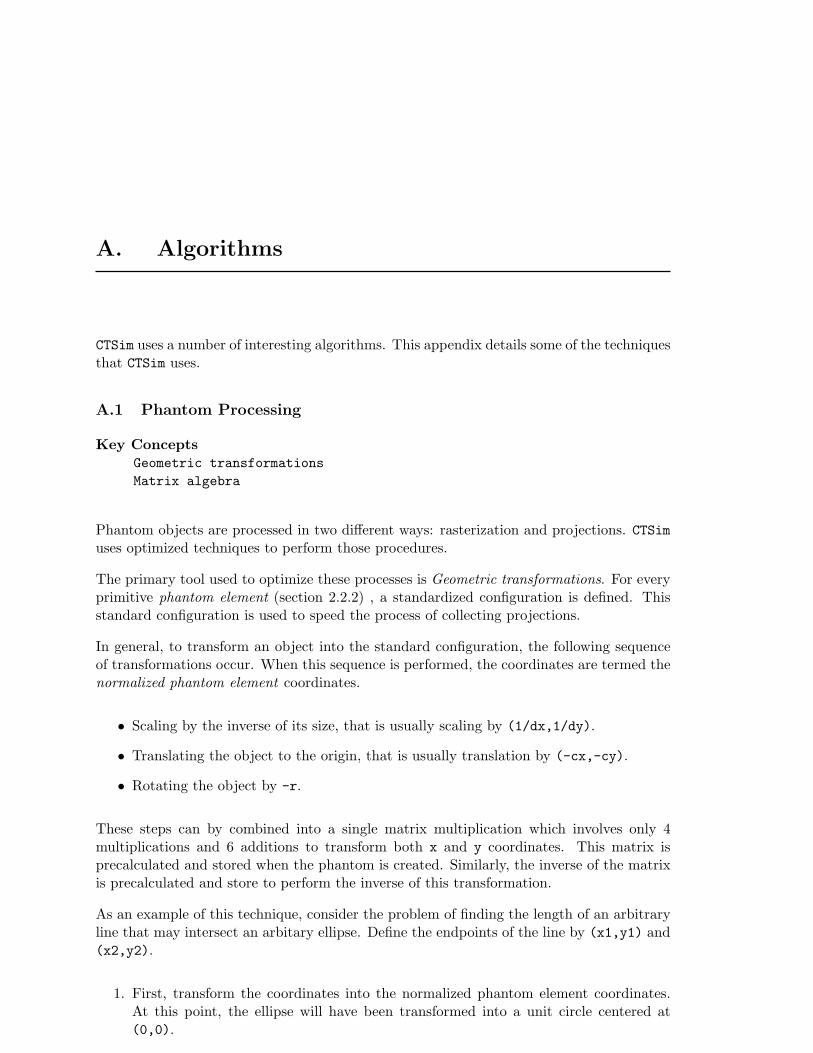
Phantom objects are processed in two different ways: rasterization and projections. CTSimuses optimized techniques to perform those procedures.
The primary tool used to optimize these processes is Geometric transformations. For everyprimitive phantom element (section 2.2.2) , a standardized configuration is defined. Thisstandard configuration is used to speed the process of collecting projections.
In general, to transform an object into the standard configuration, the following sequenceof transformations occur. When this sequence is performed, the coordinates are termed thenormalized phantom element coordinates.
• Scaling by the inverse of its size, that is usually scaling by (1/dx,1/dy).
• Translating the object to the origin, that is usually translation by (-cx,-cy).
• Rotating the object by -r.
These steps can by combined into a single matrix multiplication which involves only 4multiplications and 6 additions to transform both x and y coordinates. This matrix isprecalculated and stored when the phantom is created. Similarly, the inverse of the matrixis precalculated and store to perform the inverse of this transformation.
As an example of this technique, consider the problem of finding the length of an arbitraryline that may intersect an arbitary ellipse. Define the endpoints of the line by (x1,y1) and(x2,y2).
1. First, transform the coordinates into the normalized phantom element coordinates.At this point, the ellipse will have been transformed into a unit circle centered at(0,0).
Manual v1.0 May 1, 2002 41
CTSim 3.5.0 Manual Appendix A
2. Translate the coordinates by (-x1,-y2). The line now has the endpoint centered atthe origin. The ellipse will now have its center at (-x1,-y1).
3. Rotate the coordinates by the negative of angle of the line with respect to the x-axis.
At this point the line will now lie along the positive x-axis with one end at (0,0). The circlewill be rotated around the origin as well. At this point, it is fairly trivial to calculate thelength of the intersection of the line with the unit circle. For example, if the y coordinatefor the center of the circle is greater than 1 or less than -1, then we know that the unitcircle doesn’t intersect the line at all and stop further processing. Otherwise, the endpointsof the intersection of the line with the unit circle is a simple calculation.
Those new, intersected endpoints are then inverse transformed by reverse of the abovetransformation sequence. After the inverse translation, the transformed endpoints will bethe endpoints of the line that intersect the actual ellipse prior to any transformations.
Though this sequence of events is somewhat complex, it is quite fast since the multipletransformations can be combined into a single matrix multiplication. Further, this techniqueis amendable to rapidly calculating the intersection of a line with any of the phantomelements that CTSim supports.
A.2 Background Processing
Key ConceptsMultithreadingCritical sectionsMessage passingRe-entrant code
The CTSim graphical shell can optionally perform background processing. CTSim usesthreads as tools to achieve this functionality. Using multiple threads, termed multithreading,allows CTSim to:
• Execute a lengthy calculation in the background while the graphical shell remainsavailable for use.
• Automatically take advantage of multiple central processing units (CPU’s) in a sym-metric multiprocessing (SMP) computer.
When background processing option is turned on or when CTSim is running on a SMPcomputer, and CTSim is directed to perform reconstruction, rasterization, or projections,CTSim will spawn a Background Supervisor thread. This supervisor thread then createsa Supervisor Event Handler (supervisor). The supervisor communicates with the rest ofgraphical user interface of CTSim by using message passing to avoid issues with re-entrantcode.
The supervisor registers itself via message passing with the Background Manager which willdisplay the execution progress in a pop-up window. The supervisor also registers itself with
Manual v1.0 May 1, 2002 42

CTSim 3.5.0 Manual Appendix A
the document being processed. This is done so that if the document is closed, the documentcan send a message to the supervisor directing the supervisor to cancel the calculation.
After registering with CTSim components, the supervisor creates Worker Threads. Theseworker threads are the processes that actually perform the calculations. By default, CTSimwill create one worker thread for every CPU in the system. As the workers completeunit blocks, they notify the supervisor. The supervisor then sends progress messages tobackground manager which displays a gauge of the progress.
As the worker threads directly call the supervisor, it is crucial to lock the class data struc-tures with Critical Sections. Critical sections lock areas of code and prevent more than onethread to access a section of code at a time. This is used when maintaining the tables ofworker threads in the supervisor.
After the workers have completed their tasks, they notify the supervisor. When all theworkers have finished, the supervisor kills the worker threads. The supervisor then collatesthe work units from the workers and sends a message to CTSim to create a new window todisplay the finished work.
The supervisor then deregisters itself via messages with the background manager and thedocument. The background manager removes the progress gauge from its display andresizes its window. Finally, the background supervisor exits and background supervisorthread terminates.
This functionality has been compartmentalized into inheritable C++ classes BackgroundSupervisor,BackgroundWorkerThread, and BackgroundProcessingDocument. These classes serve asbase classes for the reconstruction, rasterization, and projection multithreading classes.
A.2.1 Advantages
This structure may seem more complex than is necessary, but it has several advantages:
• Since the background threads do not directly call objects in the graphical user interfacethread, problems with re-entrant code in the graphical interface are eliminated.
• A supervisor can parallel process with any number of worker threads to take advantageof potentially large numbers of CPU’s in SMP computers.
• Allows for continued user-interaction with CTSim while lengthy calculations are per-formed in the background.
A.2.2 Disadvantages
The above advantages are not free of cost. The disadvantages include:
• Increased memory usage.The workers threads allocate memory to store their intermediate results. When theworker threads finish, the supervisor allocates memory for the final result and col-lates the results for the workers. This collation results in a doubling of the memory
Manual v1.0 May 1, 2002 43
CTSim 3.5.0 Manual Appendix A
requirements. Of course, after collation the supervisor releases the memory used bythe workers.
• Slower execution on single CPU systems.Creating multiple threads, sending progress messages to the background manager, andcollation of results for worker threads adds overhead compared to simply calculatingthe result directly in the foreground. On single CPU systems this results in slowerprocessing compared to foreground processing. On dual-CPU and greater SMP sys-tems, though, the advantage of using multiple CPU’s in parallel exceeds the overheadof background processing.
Manual v1.0 May 1, 2002 44
B. Simple Graphics Package
Simple Graphics Package was created in 1980 by Kevin Rosenberg and is modelled afterthe hypothetical graphics library described by Foley and van Dam[1]. It is designed to beplatform-independent.
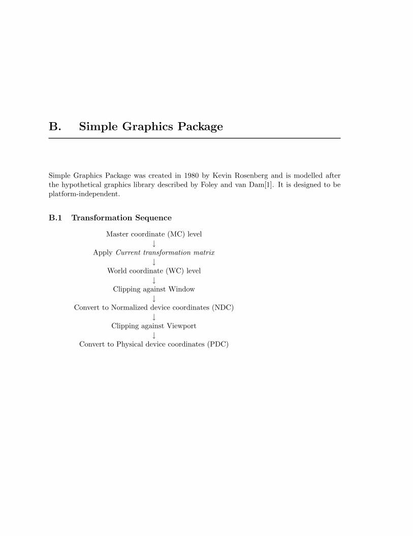
B.1 Transformation Sequence
Master coordinate (MC) level↓
Apply Current transformation matrix↓
World coordinate (WC) level↓
Clipping against Window↓
Convert to Normalized device coordinates (NDC)↓
Clipping against Viewport↓
Convert to Physical device coordinates (PDC)
Manual v1.0 May 1, 2002 45
CTSim 3.5.0 Manual Appendix B
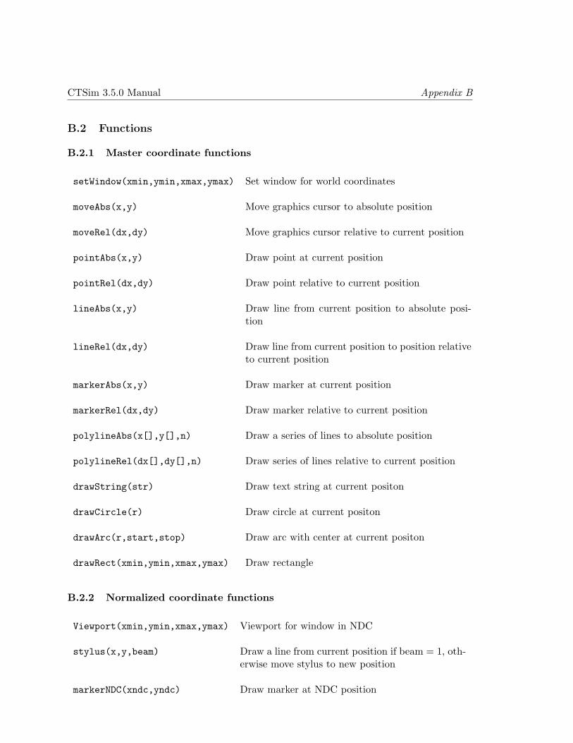
B.2 Functions
B.2.1 Master coordinate functions
setWindow(xmin,ymin,xmax,ymax) Set window for world coordinates
moveAbs(x,y) Move graphics cursor to absolute position
moveRel(dx,dy) Move graphics cursor relative to current position
pointAbs(x,y) Draw point at current position
pointRel(dx,dy) Draw point relative to current position
lineAbs(x,y) Draw line from current position to absolute posi-tion
lineRel(dx,dy) Draw line from current position to position relativeto current position
markerAbs(x,y) Draw marker at current position
markerRel(dx,dy) Draw marker relative to current position
polylineAbs(x[],y[],n) Draw a series of lines to absolute position
polylineRel(dx[],dy[],n) Draw series of lines relative to current position
drawString(str) Draw text string at current positon
drawCircle(r) Draw circle at current positon
drawArc(r,start,stop) Draw arc with center at current positon
drawRect(xmin,ymin,xmax,ymax) Draw rectangle
B.2.2 Normalized coordinate functions
Viewport(xmin,ymin,xmax,ymax) Viewport for window in NDC
stylus(x,y,beam) Draw a line from current position if beam = 1, oth-erwise move stylus to new position
markerNDC(xndc,yndc) Draw marker at NDC position
Manual v1.0 May 1, 2002 46

CTSim 3.5.0 Manual Appendix B
B.2.3 Master coordinate to World coordinate transformations
These transformation functions operate on the Current transformation matrix (CTM).
clearCTM() Sets the CTM to an identity matrix
preTranslate(x,y) Apply translation to CTM
postTranslate(x,y) Apply translation to CTM
preScale(x,y) Apply scale to CTM
postScale(x,y) Apply scale to CTM
preRotate(angle) Apply rotation to CTM
postRotate(angle) Apply rotation to CTM
preShear(x,y) Apply shear to CTM
postShear(x,y) Apply shear to CTM
B.2.4 Coordinate transformation functions
transformMCtoNDC(&x,&y) Convert from master coordinates to NDC
transformNDCtoMC(&x,&y) Convert from NDC to master coordinates
B.2.5 State functions
eraseWindow() Clears the screen
setColor(color) Set current pen color
setLinestyle(style) Set current pen style
setLinewidth(width) Set current pen width
setTextColor(foreground, background) Set text colors
setMarker(type,color) Set marker attibutes
setRasterOp(rasterOp) Set raster operator
Manual v1.0 May 1, 2002 47
CTSim 3.5.0 Manual Appendix B
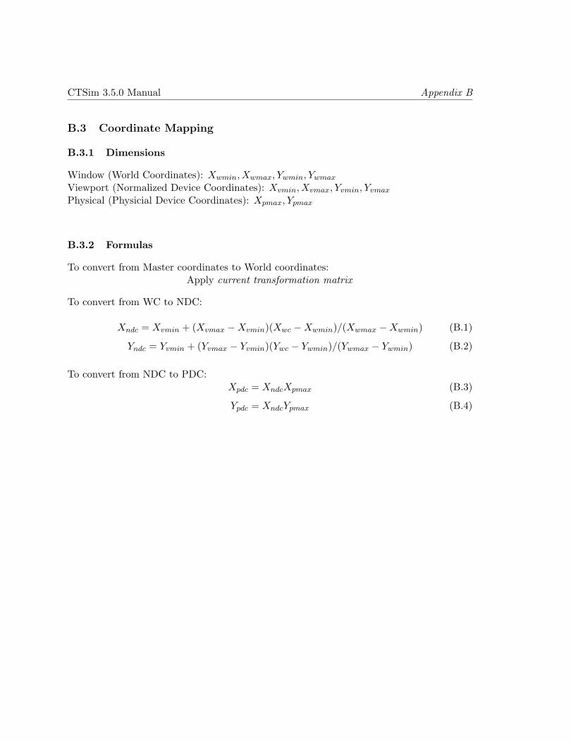
B.3 Coordinate Mapping
B.3.1 Dimensions
Window (World Coordinates): Xwmin, Xwmax, Ywmin, Ywmax
Viewport (Normalized Device Coordinates): Xvmin, Xvmax, Yvmin, Yvmax
Physical (Physicial Device Coordinates): Xpmax, Ypmax
B.3.2 Formulas
To convert from Master coordinates to World coordinates:Apply current transformation matrix
To convert from WC to NDC:
Xndc = Xvmin + (Xvmax −Xvmin)(Xwc −Xwmin)/(Xwmax −Xwmin) (B.1)
Yndc = Yvmin + (Yvmax − Yvmin)(Ywc − Ywmin)/(Ywmax − Ywmin) (B.2)
To convert from NDC to PDC:Xpdc = XndcXpmax (B.3)
Ypdc = XndcYpmax (B.4)
Manual v1.0 May 1, 2002 48

Bibliography
[1] J.D. Foley and A. van Dam. Fundamentals of Interactive Computer Graphics. Addison-Wesley, 1982.
[2] G.T. Herman. Image Reconstruction from Projections: The Fundamentals of Comput-erized Tomography. Academic Press, New York, 1980, 1980.
[3] L. Shepp and B. Logan. The fourier reconstruction of a head section. IEEE Transactionsin Nuclear Science, NS-21(6):21–43, 1974.
Manual v1.0 May 1, 2002 49

Index
Algorithms, 41Auto scale, 20
Background processing, 42
Center-Detector length, 5Command line interface, 29Conceptual overview, 2ctsim, 11ctsimtext, 29
DialogCreate filter, 13Create phantom, 13Preferences, 15Projections, 18Rasterize, 17Reconstruction, 24ReconstructionRebin, 28
Download, 39
Equiangular geometry, 6Equilinear geometry, 6
Fan beam angle, 6File types, 12Filtered backprojection, 9Focal length, 5
Graphical interface, 11
if1, 30if2, 30ifexport, 31ifinfo, 32Image
Comparison, 10, 22Export, 19Filter, 21
Installation, 39Intensity scale, 19
LAM, 29
MPI, 29
Parallel geometry, 5
Parallel processing, 9, 29Phantom
Diameter, 4Elements, 3File syntax, 2Size, 3
phm2if, 34phm2pj, 33pj2if, 35pjinfo, 35pjrec, 36Polar conversion, 23
Quick Start, 11
Reconstruction overview, 9
Scan diameter, 5Scanner
Concepts, 3Equiangular, 6Equilinear, 6Parallel, 5
Simple Graphics Package, 45SMP, 9Source code build, 39Symmetric multiprocessing, 9
View diameter, 4
Web interface, 38
Manual v1.0 May 1, 2002 50