Tero Lempiainen

Visual analysis of radio frequencyconformance test results

Faculty of Electronics, Communications and Automation

Thesis submitted for examination for the degree of Master ofScience in Technology.

01.04.2010

Thesis supervisor:

Prof. Risto Wichman

Thesis instructor:

M.Sc.(Tech.) Aleksi Heino

A’’ Aalto UniversitySchool of Scienceand Technology

aalto-yliopisto

teknillinen korkeakoulu

diplomityon

tiivistelma

Tekija: Tero Lempiainen

Tyon nimi: Visual analysis of radio frequency conformance test results

Paivamaara: 01.04.2010 Kieli: Englanti Sivumaara: 7+46

Elektroniikan, tietoliikenteen ja automaation tiedekunta

Signaalinkasittelyn ja akustiikan laitos

Professuuri: Signaalinkasittelytekniikka Koodi: S-88

Valvoja: Prof. Risto Wichman

Ohjaaja: DI Aleksi Heino

Tassa diplomityossa esitellaan visuaalinen menetelma kolmannen sukupolvenmatkapuhelimien yhdenmukaisuustestien tulosten analysointiin. Tyossa kasitellyttestit kasittavat matkapuhelimen lahettimen ja vastaanottimen ominaisuuksienradiotaajuuksisia mittauksia. Analyysimenetelma perustuu normalisoitujen mit-taustulosten graafiseen esittamiseen. Esitys mahdollistaa laitteiden keskinaisenvertailun seka vertaamisen testirajoihin. Tyossa analyysimenetelmaa sovelletaankolmen eri laitteen testituloksiin. Analyysituloksista voidaan paatella, ettamenetelma sopii kyseisen tiedon havainnollistamiseen ja analysointiin.Analyysituloksiin perustuen valitaan suoritetuista testeista suositus testijoukoksikaytettavaksi laitteiden vertailumittauksiin tuotekehityksessa. Kyseisten testientulokset osoittivat eroja laitteiden valilla.

Avainsanat: 3GPP, WCDMA, UMTS, radiorajapinnan yhdenmukaisuustesti,laatikkokuvio, laatikko-viikset-kuvio, visuaalinen analyysi

aalto university

school of science and technology

abstract of the

master’s thesis

Author: Tero Lempiainen

Title: Visual analysis of radio frequency conformance test results

Date: 01.04.2010 Language: English Number of pages: 7+46

Faculty of Electronics, Communications and Automation

Department of Signal Processing and Acoustics

Professorship: Signal processing Code: S-88

Supervisor: Prof. Risto Wichman

Instructor: M.Sc.(Tech.) Aleksi Heino

This thesis presents a visual method for analysis of third generation mobile phoneconformance test results. The tests included are radio frequency transmitter andreceiver tests. The analysis method is based on presenting the normalised mea-surement results as boxplots. The method allows benchmarking of devices andcomparing results against test limits. The method is applied to results of threedevices, which confirms that the method is suitable for visualising this type ofdata.Based on the analysis results of the three devices, a test set for comparing devicesin the product development is recommended. This set includes test cases thatrevealed differences between any of the tested devices.

Keywords: 3GPP, WCDMA, UMTS, conformance test, boxplot, visual analysis

iv

Preface

This Master’s Thesis was completed in Cellular Modem Compliance Laboratory ofNokia Devices Research & Development unit. Head of the laboratory is Aleksi Heinowho was also the instructor of this thesis. I would like to thank Aleksi for enablingthis thesis and for his devoted support during the whole project.

I also would like to thank the supervisor of this thesis, Professor Risto Wichmanfrom the Department of Signal Processing and Acoustics, for his support and advices.

Special thanks to the two last minute proof readers for their attention and ideas:Troels Forchhammer from Nokia Copenhagen, who has been my mentor in testanalysis since I joined Nokia in 2007, and Mikko Jokinen, my future father-in-law.

Thanks to my colleagues in Salo and Copenhagen for their understanding andsupport.

Many thanks also to my family for their patience and encouragement troughoutmy studies.

And finally I would like to express my greatest gratitude to my fiancee, Essi.She has given me inspiration and motivation on this sometimes stressful journey.Apologies for the long days I have spent writing this thesis.

Salo, 1.4.2010

Tero Lempiainen

v

Contents

Abstract (in Finnish) ii

Abstract iii

Preface iv

Contents v

Abbreviations and terms vi

1 Introduction 1

2 Universal Mobile Telecommunications System 3

3 Test Cases 63.1 Power Control Measurements . . . . . . . . . . . . . . . . . . . . . . 63.2 Transmit Modulation . . . . . . . . . . . . . . . . . . . . . . . . . . . 83.3 Transmit Intermodulation . . . . . . . . . . . . . . . . . . . . . . . . 103.4 Adjacent Channel Leakage Ratio . . . . . . . . . . . . . . . . . . . . 113.5 Receiver Dynamic Performance . . . . . . . . . . . . . . . . . . . . . 113.6 Adjacent Channel Selectivity and Blocking . . . . . . . . . . . . . . . 123.7 Transmit Spectrum Measurements . . . . . . . . . . . . . . . . . . . . 133.8 Receiver Spurious Emissions . . . . . . . . . . . . . . . . . . . . . . . 14

4 Analysis Methods 164.1 Normalisation of Results . . . . . . . . . . . . . . . . . . . . . . . . . 164.2 Boxplots . . . . . . . . . . . . . . . . . . . . . . . . . . . . . . . . . . 17

5 Analysis Results 195.1 Measurement Equipment . . . . . . . . . . . . . . . . . . . . . . . . . 195.2 Measurement Results . . . . . . . . . . . . . . . . . . . . . . . . . . . 20

6 Application of Analysis to Test Planning 386.1 Test Times . . . . . . . . . . . . . . . . . . . . . . . . . . . . . . . . . 386.2 Test Set Recommendation . . . . . . . . . . . . . . . . . . . . . . . . 396.3 Iterative Method for Receiver Tests . . . . . . . . . . . . . . . . . . . 40

7 Conclusions 43

References 45

vi

Abbreviations and terms

Abbreviations

2G 2nd generation3G 3rd generation3GPP 3rd Generation Partnership ProjectACK AcknowledgedACS Adjacent channel selectivityAICH Acquisition indicator channelAWGN Average white Gaussian noiseBCCH Broadcast control channelBER Bit error ratioBLER Block error ratioBS Base stationCE Communitas EuropaeCRC Cyclic redundancy checkCW Continuous waveDC Direct currentDCH Dedicated channelDPCCH Dedicated physical control channelDPCH Dedicated physical channelDPDCH Dedicated physical data channelDUT Device under testE-DCH Enhanced dedicated channelE-TFCI Enhanced transport format combination indicatorEDGE Enhanced data rates for GSM evolutionEVM Error vector magnitudeFDD Frequency division duplexingGCF Global Certification ForumGERAN GSM/EDGE radio access networkGMSK Gaussian minimum shift keyingGSM Global System for Mobile CommunicationsHSDPA High-speed downlink packet accessHSPA High-speed packet accessHSUPA High-speed uplink packet accessHS-DPCCH High-speed dedicated physical control channelI In-phaseIP Internet protocolL1 Layer 1 (physical layer)m-QAM QAM using m constellation pointsNACK Not acknowledgedOVSF Orthogonal value spreading functionPC Personal computerPCS Personal Communications Service

vii

PRACH Physical random access channelPSD Power spectral densityPTCRB PCS Type Certification Review BoardQ QuadratureQAM Quadrature amplitude modulationRACH Random access channelRF Radio frequencyRRC Root raised cosineRRM Radio resource managementRX ReceiveR&TTE Radio and telecommunications terminal equipmentSS System simulatorTCP Transmission Control ProtocolTFC Transport format combinationTPC Transmit power controlTX TransmitUE User equipmentUMTS Universal Mobile Telecommunications SystemUTRAN UMTS terrestrial radio access networkWCDMA Wideband code division multiple access

Terms

IEEE-488 A standard bus for traffic between measuring instrumentsTCP/IP Protocol for Internet trafficDownlink Transmission from network to user equipmentUplink Transmission from user equipment to networkUser equipment 3GPP Terminology for the mobile phoneMobile station 3GPP Terminology for the mobile phoneRelease 3GPP term for set of featuresSpreading factor Ratio between the chip rate and the symbol rateNode B The base station of WCDMA systemBand(here) A 3GPP designated frequency band of WCDMA systemsTest case A set of methods and parameters for testing certain

characteristics of a system

1 Introduction

Before a mobile phone ends up in the market for the consumer to use it must full-fill all the necessary regulatory and organisational requirements. In general, theregulatory requirements are mandatory because each country or region has its ownlegislation specifying which requirements different equipment have to comply. Forexample, in the European Union all radio or telecommunication devices must con-form to the requirements given in the Radio and Telecommunications TerminalEquipment(R&TTE) directive[1]. As a sign of conformity the manufacturer labelsthe products with the CE marking. The organisational requirements typically comefrom associations founded by various network operators. For example Global Cer-tification Forum(GCF)[2] and PCS Type Certification Review Board(PTCRB)[3]are the major ones operating in Europe and America respectively. Fullfilling therequirements set by these organisations will work as proof to the network operatorsthat the device will work as expected and can be accepted to sales through theoperators.

For a manufacturer to be able to declare that a device fills the necessary re-quirements, it is usually tested in many sectors including safety, interference andconformance. This thesis concentrates on the radio transmission and reception con-formance tests for UMTS WCDMA interface. UMTS or Universal Mobile Telecom-munications System is one of the third generation mobile communication systemsand wideband code division multiple access, WCDMA, is its air interface technology.UMTS is specified by the Third Generation Partnership Project(3GPP), which wasfounded by the major regional standardisation bodies in 1998 to provide a globalstandard for the third generation mobile networks. UMTS was the result of thisco-operation and since the first networks opened for commercial use in 2001 thestandard has spread almost throughout the world. An introduction to UMTS andWCDMA is given in chapter 2 of this thesis.

Besides complete specifications of the UMTS 3GPP has also specified confor-mance requirements for the user equipment and base station. These 3GPP docu-ments are often used as reference for the regulatory and organisational requirements,e.g. for the EU’s R&TTE directive. The conformance specification for the frequencydivision duplexing(FDD) user equipment[4] is the basis for the tests discussed in thisthesis. The tests are divided into multiple test cases arranged in chapters based onthe nature of the test. This thesis includes test cases from chapters 5 and 6 of theabove mentioned specification. These chapters describe Transmitter Characteristicsand Receiver Characteristics. The chapter numbers from the specification have beenincluded and used throughout the thesis. This makes it easy to refer each test caseby using the corresponding chapter number and thus avoiding the writing of thewhole name of test case. The included test cases are discussed in chapter 3 of thisthesis.

Conformance test cases are typically used for verification of a specific devicemodel to comply the requirements of a certain specification. For example, for devicesto be sold in the EU, the manufacturer should issue a declaration of conformity whichstates that the device complies to the requirements set in the R&TTE directive.[1]

2

Easiest way to show proof of compliance to the requirements is to run a set ofconformance tests defined in the harmonised standard.[5] These tests represent asubset of test cases specified in the 3GPP conformance specification.[4] The testsare typically performed in R&D phase to a limited number of samples.

The R&TTE directive also requires production control and quality system toensure conformity of each individual device. These processes are out of the scope ofthis thesis.

The manufacturers generally perform the tests to ensure that the product fullfillsthe requirements. This can lead to interpreting the test results only in the levelwhere a test case is passed or not. The result of a test case is seen as a ’pass’ ifthe measurements are inside limits or as a ’fail’ if the limits have been exceeded.The key question studied in this thesis is how to more effectively illustrate anduse the results of the conformance test cases. The chosen method should allowthe comparisons between different products and pointing out risky areas of a singleproduct. Single run of a test case typically includes only one measurement pereach set of parameters resulting in low total number of measurement results. Thispresents a challenge because conventional statistical tests rely on the sample size toachieve precision. The approach taken in this thesis is to represent the measurementresults of the conformance test cases by using a graphical visualisation method calledboxplot. The boxplot allows showing the results of several devices along with the testlimits in the same figure. The measurement results of the test cases are transformedto common scale to enable combining of data. These analysis methods are describedin detail in chapter 4.

To test and verify the usefulness of the methods, three device models were se-lected to be included as a reference. All the test cases which were decided to beincluded in the scope of the thesis were run once with each device by using threefrequency bands. The results of these tests are presented by using the discussedmethods in chapter 5 of this thesis.

The analysis results are also used to compose a group of test cases which couldbe used as a basis for test planning when time is limited. Test planning is addressedin chapter 6 of this thesis. The chapter includes discussion of a recommended testset derived from the results to use in research & development when performing allthe tests is not feasible due to the duration of the full test set.

3

2 Universal Mobile Telecommunications System

Universal Mobile Telecommunications System(UMTS) is globally one of the mostwidely used third generation mobile systems. Other comparable systems includecdma2000 mainly used in the USA and Time Division Synchronous Code DivisionMultiple Access(TD-SCDMA), which is being ramped up in China.[6] The air in-terface of UMTS is WCDMA which is based on multiple access scheme called directsequence code division multiple access, DS-CDMA. Using this scheme the alreadysource and channel coded symbol stream is expanded over a large bandwidth in aprocess called spreading. In this same process the different channels in a cell areseparated allowing multiple access using the same frequency band. Different chan-nels can be used to distinguish different UEs and there can be multiple channels perUE used simultaneously.

The spreading code bits are referred as chips and the code has the chip rate of thesystem which in WCDMA is 3.84 million chips per second, 3.84Mcps. The spreadingcodes come from a orthogonal code tree based on Hadamard codes and they areknown as orthogonal variable spreading functions, OVSFs in UTMS terminology.The spreading factor, SF is used to separate different levels of codes in the tree anddetermines the length of the spreading code. Possible values for spreading factorare SF = 2n, 2 ≤ n ≤ 9 which results in values between 4 and 512. The spreadingfactor can also be seen as the ratio of the chip rate to the symbol rate. Because thechip rate of the system is constant, the variable data rates between channels requiredifferent lengths of spreading codes. Thus more chips are used to transmit singlesymbol when spreading factor is increased. [7, 8]

The spreading process can be done by modulating the symbol stream with thespreading code. With BPSK signal this can be done by multiplication and an ex-ample of this is shown in figure 1. In the figure a bipolar signal presentation isused meaning that the signal values can be either -1 or +1. The x-axis representstime and the unit is set to symbol interval. Because the used spreading factoris 8, each symbol interval contains 8 chips. The different phases of the spread-ing/despreading process can be seen from top to bottom. The upper signal is thespreading code(+,−, +,−,−, +,−+) which is repeated for each symbol. Next isthe symbol stream, i.e. the signal to be spread. In the middle is the multiplicationproduct of the spreading code and the symbol stream representing the result of thespreading process. In the next row is the same spreading code as in the top, nowused to despread the data. At the very bottom is the multiplication product of thespread data and the spreading code. As can be seen this is the same signal that wasthe input signal. [7, 8, 9]

After spreading the signal already has the final chip rate and bandwidth. Thepower however is not necessarily equally distributed to the frequency range. Thenext phase flattens out the spectrum and also separates different cells in downlinkand different terminals in the uplink. This scrambling operation is done in com-plex multiplication for I and Q branches separately using a pseudo noise sequencegenerated for this purpose. Multiplication with the noise-like sequence transformsthe signal to pseudo noise having flat spectrum minimising interference to other

4

0 0.5 1 1.5 2 2.5 3 3.5 4 4.5 5

Despread data

Spreading code

Spread data

Symbol stream

Spreading code

−1

+1

−1

+1

−1

−1

+1

+1

−1

+1

Ts

Figure 1: Signal spreading/despreading for BPSK signal with spreading factor 8

terminals. [9]The use of wideband CDMA provides some useful benefits: Tolerance against

narrowband interference is good because of the (de)spreading process spreads theinterferer to large bandwidth so it can be effectively filtered out. Tolerance againstwideband interference is also good because of the used channelisation and scramblingcodes have auto- and crosscorrelation properties that allow effective isolation of thewanted signal. WCDMA systems also can take advantage of multipath propagationby using a RAKE receiver which consists of multiple receivers each receiving thesignal with different path delay. [7, 8, 9]

The drawbacks, or challenges of WCDMA systems come from the same principlesas the benefits. Because the same frequency is used by all the terminals in the cellthe observed noise level is increased the more transmissions are taking place in thecell. All the excess transmit power used causes unnecessary interference thus thetransmit power control must be very fast and responsive to allow operation in fadingconditions using only the necessary amount of output power. This is achieved byusing closed loop power control in which the base station provides terminals withpower control commands based on the measured signal to interference ratio. Thepower control cycle is done with 1.5kHz rate which effectively eliminates fading interminal point of view provided that the maximum output power is not reached.[7, 8, 9]

UMTS was first introduced to one frequency band pair for FDD use. The uplinkand downlink bands were centered around 2100MHz. This band still is the mainband in Europe and Japan but additional bands have been specified in order toefficiently use the radio spectrum and to adapt to regional regulations. Even allthe bands listed in table 1 are not yet physically in use new bands are studied andexpected to be included in new versions of specifications. [7]

3GPP specifications of UMTS have evolved since they fist introduced in 2000.3GPP uses a system of releases to allow addition of features while still providingstable specifications for product development. This means that the manufacturer

5

Table 1: 3GPP WCDMA FDD frequency bands with uplink and downlink frequen-cies. Also geographical areas of use are stated where known. [10, 11]

Name Uplink [MHz] Downlink [MHz] AreaBand I 1920-1980 2110-2170 Europe and AsiaBand II 1850-1910 1930-1990 USA and AmericasBand III 1710-1785 1805-1880 Europe, Asia and BrazilBand IV 1710-1755 2110-2155 USA and AmericasBand V 824-849 869-894 USA, Americas and AsiaBand VI 830-840 875-885 JapanBand VII 2500-2570 2620-2690 New 3GPP band(Global)Band VIII 880-915 925-960 Europe and AsiaBand IX 1750-1785 1845-1880 JapanBand X 1710-1770 2110-2170 New 3GPP band(USA)Band XI 1427.9-1452.9 1475.9-1500.9 New 3GPP band(Japan)Band XII 698-716 728-746 New 3GPP band(USA)Band XIII 777-787 746-756 New 3GPP band(USA)Band XIV 788-798 758-768 New 3GPP band(USA)

of the UE must declare which release the UE is compliant to. All the features ina certain release are not mandatory but using features of a newer release in UEdeclared to be older is not allowed. The most important releases from TX/RXconformance test point of view are currently R99 specifying the baseline WCDMAfeatures, R5 in which HSDPA was introduced and R6 which includes also HSUPA.[12]

6

3 Test Cases

Test cases included in this thesis are a subset of test cases specified in [4]. Allincluded test cases belong to chapters 5 or 6 of the specification representing ra-dio transmission and reception tests. These chapters were selected because theydescribe the fundamental requirements for RF performance. The specification alsolists a number of test cases for other aspects of the radio interface such as Layer1 performance(ch.7), radio resource management(ch.8), HSDPA performance(ch.9)and HSUPA performance(ch.10). Part of the Layer 1 performance test cases havebeen analysed in special assignment [13] using partly the same methods that areused in this thesis.

The test cases in question are specified to exclude the antenna performance bystating that the test system is connected to the DUT by an electrical conductor.This allows the test environment to be controlled more accurately as the air interfaceis left out. Conformance tests for antenna performance are specified in a separatedocument[14].

The environmental conditions of the DUT are controlled and some tests arespecified for extreme conditions in addition to normal conditions. Varied conditionsinclude temperature and supply voltage of the DUT. Normal temperature is nom-inally +25 ◦C where low and high extremes are −10 ◦C and +55 ◦C. Voltages aretied to the nominal battery voltage indicated by the manufacturer. When a powersupply is used, normal testing voltage is the nominal voltage, low voltage is 0.9×nominal and high voltage is 1.1× nominal. Humidity is not varied but it is requiredthat relative humidity of the test environment is between 25% and 75%. [4] Theextreme conditions are tested in all four combinations so environmental conditionscan be divided into five groups:

1. Normal conditions (NC)

2. High temperature, high voltage (HTHV)

3. High temperature, low voltage (HTLV)

4. Low temperature, high voltage (LTHV)

5. Low temperature, low voltage (LTLV)

In the following chapters test cases are grouped by the type of measurementinstead of the common way of arranging them to the order they are listed in thespecification. For identification and reference the original names and chapter num-bers are also included and used throughout the thesis.

3.1 Power Control Measurements

This group includes test cases that measure transmit power of the UE. The upperend of transmitter dynamic range is evaluated with maximum output power testcases. The tests specify requirements for output power when the UE is transmitting

7

at full power. The UE must comply to the limits according to which power classit is assigned. Power class is directly related to the maximum power output theUE can produce and is specified by the manufacturer. Current commercial UEsare power class 3 with nominal maximum output power of 24dBm or power class4 with nominal maximum output power of 21dBm. Higher output power can helpimproving transmission data rates or enabling communication in weak coverage areassuch as areas far away from the base station. [11]

Test case 5.2 specifies requirements for all UEs using only features from release99. Test is conducted by simply having the UE transmit at full power and measuringthe output power. [4]

HSDPA in 3GPP release 5 specifications include additional control channel, HS-DPCCH, which is not synchronous with the release 99 channels transmitted in par-allel. This results in higher peak-to-average ratio in uplink. Taking this into consid-eration 3GPP has specified relaxed requirements for time slots HS-DPCCH is in use.The target power level is the same, but the lower limit is reduced. The amount ofreduction is depending on the ratio of HS-DPCCH and uplink data channel DPDCHamplitudes and is 0, 1 or 2dB. For higher amount of control data the reduction islarger. Test case is divided to four sub-tests based on channel configuration. Thetest case number for maximum output power with HS-DPCCH is 5.2A. [4, 11]

For release 6 two new test cases were specified. The reasons are similar toHSDPA case explained above, and since release 6 includes HSUPA transmissionas an additional feature the amount of control channels and code domain channelamplitude combinations is even higher. Release 6 test case numbers for maximumoutput power in [4]are 5.2AA for UEs without HSUPA but with HSDPA and 5.2Bfor UEs supporting both HSDPA and HSUPA. These test cases are also divided intosubtests based on uplink channel power allocation.

The open loop power control is only in use when the UE starts the transmissionand is not in the control of the node B. The requirements are given in test case 5.4.1Open Loop Power Control in the Uplink. The functioning of open loop power controlensures that the UE does not create excess interference in the cell but starts with theminimum power when requesting a radio connection. The test procedure is simplyto measure the power of the random access channel(RACH) preamble when UE isinitiating connection. The measurement is done with three power levels from receiversensitivity level to upper dynamic end. The tolerance in every measurement is ±9dBfor tests in normal environmental conditions and ±12dB for extreme conditions.[4, 8]

Test case 5.4.2 tests functionality of inner loop power control of the UE. Thefunctioning of this fast closed loop power control procedure is essential in WCDMAnetworks since excess error in transmit power control results e.g. in capacity lossesor call drops. Using inner loop power control the transmit power of UE is controlledby node B via transmit power control (TPC) commands sent via control channel.Value of TPC can be either 0, -1 or +1. The stepsize is determined by systemparameter ∆TPC which is transmitted with other system information on BCCH.Possible values are 1dB and 2dB. There are two possible modes for power control,power control algorithm 1 with full 1500Hz one command per timeslot resolutionand power control algorithm 2 with 5 TPC commands grouped together resulting in

8

300Hz resolution. Only algorithm 1 is tested in this test case. During the test caseTPC commands are sent in five different patterns. First three patterns contain onlyone type of command from the possible values of -1, 0 and +1. Two more patternsare used to verify slower rate of TX power. These patterns consist of repetitions offour commands of zeros followed by either -1 or +1 depending on the pattern. Therequirements are defined in [4] for power change after each TPC command and alsofor total change after 10 consecutive pattern repetitions.[4, 11]

Test case 5.4.3 measures the minimum controlled output power of the UE. Thisrequires that both inner loop and open loop power control indicate minimum trans-mit power is required. It is important that UE is capable of operating also at lowoutput powers because any excess power transmitted reduces system capacity.

Test case 5.4.4 out-of synchronization handling of output power sets requirementsfor UE’s responses for DPCCH quality changes. The UE shall monitor the DPCCHquality at all times and when the quality drops below a certain threshold the UEshould stop transmitting in 40ms period. Again when the DPCCH quality improvesthe transmitter must be activated in 40ms. The purpose of the test case is to makesure UEs out of synchronisation do not cause interference to other communicationin the cell. The root cause for the interference would be errors in transmission ofTPC commands as the UE’s transmit power would not be in the control of node Bany longer. [4]

Test case 5.5.1 contains measurement of output power when UE is not transmit-ting. This power should obviously be as low as possible. Excess output power whennot transmitting increases interference which decreases overall system capacity. [7]This test case is usually measured as part of test case 5.5.2.

Test case 5.5.2 specifies requirements for transmit on/off time mask. Outputpower levels are measured during and between random access channel preambles.Transmit on power requirements are applied to the power measured during preambleand transmit off requirements to the power measured between preambles. There aretransition periods of 50µs between TX on and TX off power measurements centeredat the edges of preambles. [4]

3.2 Transmit Modulation

The measurements of error vector magnitude(EVM) and frequency error are done byusing the Global In-Channel Tx-Test described in [4], Annex B. This method usesreference signal generated by the test system which is filtered with pulse shapingfilter and compared to the actual transmit signal produced by the UE filtered withthe same type of filter. The filter is root raised cosine(RRC) type with bandwidthof 3.84MHz and roll off factor α = 0.22. The parameters of the reference and theactual transmit signal are varied in order to achieve best fit between the two signalsso that their difference is minimised. Following parameters are varied for the TXsignal: frequency, timing and phase. The reference signal is only varied by alteringcode domain amplitude. The minimum measurement interval is one timeslot exceptfor test cases with HS-DPCCH enabled. For those test cases shorter measurementinterval is used because the code powers can vary during one timeslot period. [4]

9

Single test case 5.3 is dedicated for measuring frequency error of the UE trans-mitted signal. Reference for the UEs transmit frequency is the received signal fromnode B so the test also covers receiver’s ability to track the signal and provide acorrect reference for the transmitter. The test is done at receiver sensitivity leveland the test requirement is ±(0.1ppm+10Hz). For example in band I middle channelwith center frequency of 1950MHz this requirement is ±205Hz. [4]

Figure 2: Error vector in complex plane.

The quality of modulation is mainly measured by the error vector magnitude,EVM. Error vector is the difference between the ideal vector and measured signal.Figure 2 shows the concept in the complex plane. It also shows how the error vectorcan be seen as composed from phase and amplitude errors. The requirements forEVM are specified as RMS power ratios between the error vector and the referencevector. The formula for EVM value after [4] is

EV M =

√

√

√

√

∑

N−1

v=0|Z ′(v) − R′(v)|2

∑

N−1

v=0|R′(v)|

2∗ 100% (1)

where Z ′(v) and R′(v) are the varied transmitted and reference vectors and N isthe number of samples in the measuring interval. The modulation used in all theEVM tests included is QPSK so there are four constellation points. The limit forall EVM tests is 17.5%. The measured EVM consists of nonlinearities cumulatedover the whole transmitter path. Local oscillator leakage in the modulator as wellas asymmeries in the baseband I and Q paths can cause increase in EVM. Also theRF output power amplifier distorts the signal especially when the saturation levelof the amplifier is approached. [15, 16]

10

Test case 5.13.1 is the basic test of EVM applicable for all UEs starting fromR99. The test case is conducted with two output power levels: maximum and-18dBm. Test case 5.13.1A is the HSDPA equivalent of 5.13.1 using HS-DPCCH asmeasurement channel. This test case is applicable for R5 UEs supporting HSDPA.The test case includes also measurements with the two aforementioned power levelsbut in addition the measurement is repeated in four different phases of HS-DPCCHtransmission including two measurements with HS-DPCCH transmitting at highestlevel and two measurements with HS-DPCCH transmission off.

Test case 5.13.1AA is much like the previous test case but it has additional re-quirement for phase discontinuity between the transition periods when HS-DPCCHtransmission is switched on and off. The measurement of EVM is done, as describedabove, for the four measurement positions. The resulting phase discontinuity is thencalculated between the first and last pairs as the difference in the absolute phasevalues of the transmitted signal used in generating minimum EVM. Test case isapplicable for R6 and later releases for UEs supporting HSDPA.

Test case 5.13.3 UE phase discontinuity measures changes in phase between twotimeslots. The measurement is done as described above but for two whole consec-utive timeslots. This test is done for the full dynamic range of the UE transmitterby starting from the maximum TX power and gradually setting the UE to the min-imum output power repeating TPC commands in a predefined pattern of [-1 -1 -1-1 -1 +1 +1 +1 +1]. This results in a total change of 1dB per 9 timeslots. Whenthe minimum output power has been reached the power is gradually increased tomaximum by repeating the inverse TPC pattern: [+1 +1 +1 +1 +1 -1 -1 -1 -1].EVM is measured for all timeslots and phase discontinuity calculated between allthe consecutive timeslots.

A separate test case, 5.13.4, is specified for measuring PRACH preamble quality.PRACH preamble is used by the UE in the random access procedure to initiate thenetwork access on layer 1. During the process UE sends preambles to node B troughrandom access channel(RACH) until a positive acquisition indication is receivedfrom the acquisition indication channel(AICH). Only after this process the randomaccess message containing details about the wanted connection can be transmittedto the node B and connection can be established if allowed by node B. During thetest used RACH sub-channel, PRACH signature and AICH transmission timing areselected randomly from a predefined set and the measurement is repeated ten timeswith different parameters. The quality metrics include EVM and frequency error.In addition the detected access slot and signature must be correct. [4, 8]

3.3 Transmit Intermodulation

Test case 5.12 measures the intermodulation effects of the transmitter when an inter-fering signal is present in the antenna. The test is performed with four frequenciesof interfering sinusoidal continuous-wave signal: 5 and 10 MHz above and below thecarrier frequency. The level of the interferer is 40dB below the transmit power level.Each interferer offset potentially produces two intermodulation products, one aboveand one below the carrier frequency. The intermodulation attenuation requirements

11

are expressed as the ratio of the root raised cosine(RRC) filtered mean power ofthe transmit channel signal to the RRC filtered mean power of the intermodulationproduct. The requirements are -31dB for 5MHz offsets and -41dB for 10MHz offsets.[4]

3.4 Adjacent Channel Leakage Ratio

Test cases 5.10 to 5.10B measure the leaked power ratio on adjacent channels. Thepurpose of the test case is to limit the interference the UE produces to commu-nications on other UMTS channels. A particular scenario when adjacent channelleakage impacts network performance is when the UE is transmitting to a far awaybase station(BS) with high power and there is another BS using adjacent channel inclose vicinity of the UE. The key components in a transmitter that influence ACLRare the power amplifier and the modulator. Particularly third order distortion in themodulator causes rise in leaked power. Generally improving ACLR by modulatorlinearity causes more power consumption which is always a drawback in a batteryoperated device. Finding a proper compromise with filing the requirements andpower consumption is thus an important part of transmitter design. [11, 15]

The test is done by first measuring the root-raised-cosine(RRC) filtered powerof the actual transmit channel and then comparing the similarly filtered power ofadjacent channels to this power. The roll-off factor of this filter simulating that of areal receiver is r = 0.22 and bandwidth 3.84MHz. Measurements are made for thefirst adjacent channels 5MHz above and below UE transmit frequency as well as thesecond adjacent channels 10MHz above and below the TX frequency. During themeasurement the UE is transmitting with full output power.

Test case 5.10 uses basic R99 features and is required for all types of UEs. Testcase 5.10A is valid for all UEs supporting HSDPA and is done with HS-DPCCH ac-tive. This test case includes measurements with four power allocation configurationsbetween uplink data and control channels. Otherwise requirements and proceduresare the same as with 5.10. Test case 5.10B uses also E-DCH in addition to HS-DPCCH. This test is only for R6 UEs supporting HSDPA and HSUPA and includesfive subtests with different uplink channel power allocation configurations.

3.5 Receiver Dynamic Performance

The performance of RF front end of the receiver is mainly evaluated by bit errorratio(BER) tests. 3GPP specifies tests to be done with UE test loop mode 2 usingUL 12.2kbps reference measurement channel. This loop mode functions as follows:The system simulator(SS) sends the UE test data which the UE loops back withsymmetrical DL channel. The SS compares the received data to the original andcalculates BER. By using this method all basic functions of WCDMA networks belowlayer-2 are actually in use including cyclic redundancy check, tail bit attachment,convolutional coding, interleaving and rate matching. This results to the fact thatthe bit errors are not independent. BER tests are sometimes defined so that they

12

circumvent channel coding which results in independence of the errors but this isnot the case with the BER tests in question. [4, 8, 18]

In test case 6.2 the receiver is tested with very low input power. The power level isthe minimum a UE is required to work and called reference sensitivity level. The testis conducted by using BER test with downlink power set to the reference sensitivitylevel. The requirement is to achieve 0.1% BER. Since this test simulates transmissionin great distance from node B output power of the UE is set to maximum. Testingthe sensitivity of a receiver is important because the specified sensitivity is used inplanning coverage of UMTS cells and it is expected every UE works also at the edgeof the cell coverage. As the received signal power is very low the noise present inthe receiver is the most critical parameter of receiver design. The noise is a sum ofmultiple sources including thermal noise, input amplifier noise, phase noise of thelocal oscillator and leaked transmitter power. [8, 11, 15]

Test case 6.3 stresses the UE in the other dynamic end compared to 6.2. Inthis test the input signal is at maximum level the UE is required to work. Transmitpower is set to a predefined value below maximum. This test is also conducted usingBER test and the requirement is to achieve 0.1% BER.

For a HSDPA terminal supporting 16QAM there is one additional test for maxi-mum input level. This is because of the need to more accurately preserve the phaseand amplitude with this higher modulation scheme. Test case 6.3A is similar to 6.3but downlink uses HSDPA transfer with 16QAM signal. Also the test is not done asa BER test but as a throughput test. Throughput is calculated by using acknowl-edged/not acknowledged(ACK/NACK) messages from the UE and the requirementis to achieve 700Kbps or more whereas the nominal bit rate for the used channelconfiguration is 777Kbps. [4, 11]

3.6 Adjacent Channel Selectivity and Blocking

Adjacent channel selectivity(ACS) is the measure of how large power level can beused at the adjacent channel compared to the received power. The UE is required tooperate with ACS of 33dB. This means that the power used in the channel adjacentto UE’s received channel is 33dB greater than the received signal power. The testcase is done with two power levels starting from rel-5 UEs and for one level for release99 and 4 UEs. 3GPP test case numbers are 6.4 and 6.4A. The correct operationof the UE is determined by using the BER test while simulated WCDMA signal isused as interferer. The conditions which require good ACS are typical when two ormore operators are sharing the same area and frequency band. The ACS is mainlydetermined by the RF and baseband filtering in the receiver. [11]

Blocking tests are covered in chapter 6.5. Blocking characteristic is a measure ofthe receiver’s ability to receive a wanted signal at its assigned channel in presence ofan unwanted interfering signal[4]. Test case 6.5 is separated into three different typesof blocking tests: in-band-, out-of-band- and narrowband blocking all measuringBER when an interfering signal is present at the receiver. The filters in the receivercarry the biggest responsibility in complying to the blocking requirements but alsononlinearity of the receiver can cause impaired performance. [15]

13

During the in-band blocking test the interfering signal is a simulated WCDMAsignal with frequency offsets -10MHz, +10MHz, -15MHz and +15MHz to the usedreceive band’s center frequency. The adjacent channels with offsets -5MHz and+5MHz are tested in the ACS test case described above. Each interfering signal istested separately. This test is required in order to make sure the UE is capable ofoperating in presence of other WCDMA systems in the same band. The level of theinterfering signal is -56dBm with ±10MHz offsets and -44dBm with ±15MHz offsetswhile the received signal level is set to reference sensitivity +3dB.

Narrowband blocking is only specified for certain frequency bands which arepotentially used together with some narrowband second generation mobile networksuch as GSM. Currently this means FDD bands II, III, IV, V, VIII, X, XII, XIIIand XIV. The used interferer is GMSK modulated to simulate GSM signal and theoffset from the WCDMA carrier is 2.7MHz for bands III and VIII and 2.8MHz forall the other tested bands. The level of the interferer is also depending on the bandbeing -56dBm for bands III and VIII and -57dBm for the other bands. The receivedsignal level is adjusted to 10dB above the reference sensitivity level.

Out-of-band blocking includes sinusoidal interferer with frequency range of 1MHzto 12750MHz excluding the frequencies tested on other blocking tests or the ACStest. The level of the interferer depends on the frequency band under test andthe distance from the carrier but is always between -44dBm and -15dBm while thetransmitted signal level is 3dB above the reference sensitivity level. Frequency of theinterferer is swept in 1MHz steps and for each frequency a BER test is made. If themeasured BER value is above the threshold or the call is disconnected an exceptionhas happened. The frequency of the interferer is recorded for later analysis. Thenumber of allowed exceptions are limited and depend on the frequency range of theinterferer and band in use.

The exception frequencies from the out-of-band test are tested in a separate testcase, 6.6, with similar blocking test but with the level of interfering signal set to-44dBm. UE received signal power is the same as in the blocking test, 3dB abovereference sensitivity.

3.7 Transmit Spectrum Measurements

This chapter includes tests for occupied bandwidth and unwanted emissions fromthe transmitter. The positioning of test cases in the frequency domain is presentedin figure 3.

Test case 5.8 specifies requirements for UE transmitted signal bandwidth. Thebandwidth must be below 5MHz. The occupied bandwidth is defined to be thefrequency range containing 99% of the total transmitted power. Total power ismeasured in minimum of 10MHz band around the center of the carrier. [4]

In the transmitter spurious emissions are formed as a result of non-linearitiessuch as harmonic and intermodulation distortion. It is possible that such unwantedproducts fall into frequencies they can cause interference to other equipment ornetworks.

For frequencies 2.5MHz - 12.5MHz away from the center frequency of the TX

14

channel transmitter requirements are defined in test cases 5.9 to 5.9B. The require-ments are specified relative to the RRC filtered carrier power and depend on themeasurement frequency. The measurement filter bandwidth is 30kHz for frequen-cies 2.5MHz to 3.5MHz away from the carrier center and 1MHz for the rest of thecovered spectrum. Test case 5.9 uses basic R99 functionality where test case 5.9Auses HS-DPCCH for downlink and 5.9B also uses E-DCH for uplink. The basicrequirements are the same in all the tests.

Test case 5.11 specifies requirements for frequencies more than 12.5MHz awayfrom the carrier center frequency. The measured spectrum starts from 9kHz andends to 12.75GHz. Measurement bandwidth is 1kHz for frequency range 9kHz -150kHz, 10kHz for 150kHz - 30MHz, 100kHz for 30MHz - 1GHz and 1MHz for1GHz and above. The minimum requirements for these ranges are -36dBm for allexcept the highest range for which the requirement is -30dBm.

In addition to these general requirements there are specific additional require-ments for UEs using certain bands. These are guard bands for protecting co-existingnetworks from excess interference. The measurement bandwidths and requirementsare specified in detail in [4]. Usually when it is possible that a narrow band systemsuch as GSM is present in the same area the possible frequency range for that sys-tem is measured with narrow filter with bandwidth of 100kHz or 300kHz and thelevel of allowed emission is lower than in the general test. Similarly in cases whereadditional WCDMA bands are present the assigned frequencies are measured withbandwidth of 3.84MHz representing the bandwidth of a WCDMA channel.

Figure 3: Emission test cases presented in relation to distance from the TX carriercenter frequency fc.

3.8 Receiver Spurious Emissions

Spurious emissions of the receiver are measured in test case 6.8. The requirementsare specified for frequencies 30MHz - 12.75GHz with 100kHz measurement band-width below 1GHz and respectively bandwidth of 1MHz above 1GHz. The maxi-mum level allowed for the former range is -57dBm and for the latter -47dBm. Duringthe test the UE is not transmitting so the measurement results should not have in-terference from the transmitter. As above in transmitter test this test case has

15

also specific requirements for multiple guard bands including the UE transmit andreceive bands. The limit for the TX and RX bands is -60dBm for measurementbandwidth of 3.84MHz. [4]

16

4 Analysis Methods

4.1 Normalisation of Results

Because of differences in measured units, limits and test case parameters it is usefulto use some normalised scale in which all the results are presented. One approachis to use the 3GPP specified limits as a basis. In addition to the limits an ideal ortarget value is required in the process. The generation of normalised values can beexpressed as

xi ≥ x : xi =xi − x

lu − x(2)

xi > x : xi =xi − x

x − ll(3)

where xi is the result from measurement i, xi is the normalised result, x is the idealvalue, lu is the upper limit and ll is the lower limit. In this scale 0 will representan ideal value and -1 and 1 will be the lower and upper limits. Anything betweenthem shall be a passing result whereas failed tests will have absolute values over 1.This method is a modified version of an method used in the laboratory for 2G testanalysis. [17]

The advantage of using this kind of normalisation is that it is easy to look at thedata and spot any results that are outside the limits or close to them. The biggestdisadvantage is that the true margins to the limits cannot be directly observed. Onehas to know what is the ideal value and what are the limits in order to return theoriginal information which could be e.g. power levels in dBm. Most useful uses forthis normalisation are the test cases with several similar test steps with differentlimits. Without the normalisation it would make no sense to group these results to-gether. Even when using limit-normalisation the grouping of results from differenttest cases can cause problems if the distributions of the results are very differentin respect to limits. This is most likely to happen between different types of tests.If test cases have significantly different distributions on the limit-normalised scalegrouping them should not be done when comparing products. The actual perfor-mance difference of the devices may not be observed if the combined distributionhas many peaks due to the different test cases. Also the number of results shouldbe similar when combining results of multiple test cases since test case with largenumber of results can rule over ones with less results. If the purpose of the analysisis only to check the margin to limits then this problem does not exist but it is notpractical to include results of very different test cases into one group.

In some cases above method is not practically possible since there is no cleartarget but the ideal result is as low or as high as possible. This is typical to someemission and output power test cases where results and limits are expressed asdecibels and test cases are having only high limit. It is useful to simply scale theresults so that the limit is 0 dB. When operating on the decibel scale this procedureincludes only subtraction or summation of the limit value from the measurementresults. This normalisation allows the margin to the limit to be clearly visible usingthe same units as the original measurement data.

17

4.2 Boxplots

The target of this work is to provide a somewhat simple process of exploring thetest results allowing comparisons and risk analysis. This can be achieved by usingof a graphical presentation and visually exploring the data. Boxplot is a visual ex-ploratory data analysis method suggested by John Tukey.[19] The exploratory dataanalysis is a branch of statistics where the data is used to formulate the actualhypothesis in contrast to confirmatory data analysis which relies on hypothesis test-ing. Boxplots are suitable for the needs of this work because they can be used forpresenting multiple datasets in a compact presentation and they can be comparedto each other or to a known reference.

When generating a boxplot the corresponding data set is first ordered in increas-ing order. This data set is then divided into four equal parts so that these partsinclude equal number of data points. The three dividing values are called quartilesof which the middle one is also the median of the data set. The lower and upperquartiles are used as the lower and upper limits of the box in graphical representa-tion whereas the median is drawn as a line inside the box. The distance between thelower and upper quartiles is called the interquartile range and it also is the lengthof the box. This range is used in finding outliers in the data which are defined to bethe samples that lie more than 1.5 times the interquartile range away from the edgesof the box. In graphical representation outliers are usually marked with asterisk orother symbol so that they are clearly separated from the rest of the data. The boxplot is finalised by showing the smallest and largest values of the data set, excludingoutliers, as whiskers or lines attached to the box.

Figure 4: A boxplot created from 1000 samples with standard normal distribution

18

Figure 5: A histogram made of the same 1000 samples as the boxplot in the previousfigure

Figure 4 shows an example of a boxplot generated from a set of 1000 samples withstandard normal distribution. The histogram of the same data is shown in figure 5.Boxplot shows the shape of the distribution in a very condensed presentation andthus it is effective in data visualising allowing many data sets to be included in acompact space. From this example some typical properties of boxplots can be seen.The median value, shown as a line inside the box, is at the middle and the box issymmetrical around this value. This shows that the underlying distribution peaksat the middle and symmetrically tapers towards high and low values. There arealso a few outliers and a pair of whiskers showing the smallest and largest valuesof the data. The motivation for separating the outliers is that they are potentialmeasurement errors or otherwise do not fit in the data. It is quite natural to havesome outliers in boxplots. In this example the outliers are very close to the whiskersso they are not likely very different from the rest of the data. If there was a groupof outliers at a far distance from the whisker, the distribution would probably havetwo peaks. In that case the data set could be partitioned further, if possible, to findout the underlying cause.

When the data is having some anchor points it can be useful to include theanchors in the graph. In the following chapters the data is normalised by the testlimits so it is useful to include the limits and the ideal value(if used) in the figures.This allows the reader to see the margin to the limit.

19

5 Analysis Results

5.1 Measurement Equipment

The test setup consists mainly of the test system and the device under test withwired RF connection between the UE antenna connector and the assigned port inthe test system. Other parts include RF-shielding, temperature chamber, voltagesource, adapters, cables and possibly other accessories. When testing radio accessproperties of mobile devices it is important that testing takes place in an environmentwith no external disturbances which could affect test results. RF shielding the roomthe test system is located in can be used to achieve this.

The test system provides the UE with signals and environment that resemblethose of live networks. Test environment is specified in [20]. This specificationincludes information about logical, transport and physical channels, test frequenciesand message contents.

Test system, as defined in [4], annex A is ”A combination of devices broughttogether into a system for the purpose of making one or more measurements on aUE in accordance with the test case requirements. A test system may include one ormore system simulators if additional signaling is required for the test case.” Systemsimulator is defined in the same document as ”A device or system, that is capableof generating simulated Node B signaling and analyzing UE signaling responses onone or more RF channels, in order to create the required test environment for theUE under test. It will also include the following capabilities:

1. Measurement and control of the UE TX output power through TPC commands

2. Measurement of RX BLER and BER

3. Measurement of signaling timing and delays

4. Ability to simulate UTRAN and/or GERAN signaling”

In addition to a system simulator test systems usually include fading simulators,generators for interfering signals and a power meter. Different tests also requiredifferent paths between instruments so a routing unit is required.

The test system used for the measurements was Anritsu ME7873F TRx/PerformanceTest System[21]. This system consists of multiple discrete instruments and it is ca-pable of performing all the test cases included in this work. The block diagram ofthe system is presented in figure 6.

RF units(combiner, switch and interface units) handle the routing, amplification,combining and filtering of RF signals between the other units and the device undertest. These units are controlled by the RF switch driver.

The signaling tester provides most of the functionality of a system simulatordefined above. The functions include simulation of base station(Node B) signaling,higher level call processing procedures to set up and manage calls and measurementsof block error ratios. An additional device directly connected to the signaling testeris used for measurement of bit error ratios.

20

Signal generators are mainly used for providing interference signals to the simu-lated radio channel according to test case definitions. Vector signal generators pro-duce the simulated WCDMA and 2G signals along with noise whereas CW signalgenerator is used for sinusoidal interferers. One vector signal generator is dedicatedfor use with the fading simulator. Together the units provide the simulation offading radio channel used in layer 1 demodulation performance tests.

The TX tester unit is used for measurement of the properties of DUT TX sig-nal. Different metrics like power levels, EVM, frequency errors or bandwidths aremeasured with this equipment. It is also used for system self check and adjustment.

DC supply is used for providing the DUT with constant testing voltage during thetest run. Temperature chamber is used for keeping the DUT at correct temperatureduring the test.

The units in test system are controlled by the system controller, which is a PCequipped with special software for remote control of the devices. The remote con-trolling is done via IEEE-488 bus and Ethernet using standard TCP/IP connection.The controller PC software user interface allows the selection of test cases and theoperation of the system is fully automated after the user starts the tests from theuser interface. After the completion of the tests report files are stored in the PCshard drive. [21]

5.2 Measurement Results

The measurement data used in this thesis is gathered from three test rounds eachdone with a somewhat different device. The results not necessarily represent the finalperformance of any real device but they are actual measured results. During thisthesis the devices are referred only as DUT#1, DUT#2 and DUT#3. From eachtest round the results for frequency bands FDDI, II and VIII were used becausethese were available for all the devices. DUT#1 is release 5 compliant while theothers are release 6 compliant. In practice this means that some test cases specificto these releases are not available for all the devices, e.g. all the HSUPA tests areonly done for DUTs #2 and #3. All test cases are from [4] chapters 5 and 6. Theselection of individual test cases from these chapters is done as wide as possible byusing every test case available in the system and supported by the devices. The testsare done in all the environmental conditions that are required in the specificationfor each test.

The actual process of turning test system reports into graphics was started bycollecting all the data into Microsoft Excel worksheet. The data was organised andfiltered so that essential parameters and measurement results remained while otherdata was discarded. The normalised values or margins were then calculated andthe resulted data set was exported to Minitab statistical software for creating thegraphics.

Boxplots or histograms were done for all test cases separately by using differentvariables such as band, environmental condition or test step in grouping of the data.Different groupings were used until a valid combination of separating variables wasfound. The justification for a set of variables was to have similar data points inside

21

Figure 6: Block diagram of the Anritsu ME7873F test system.[21]

the boxes still keeping the number of boxes reasonable. In practice this meant 1–3separating variables for each test case. If a test case included different types ofmeasurements(e.g. EVM and frequency error) they were given separate graphs. Forsome test cases there were multiple approximately equally good sets but only onewas selected to be used. The ordering of the separating variables in the figures variesand it is chosen in each test to emphasise the findings made. For some tests onlyseparating variable used was the DUT because others did not give any additionalvalue to the presentation. From the selection of test cases only those showing somepossibly interesting information were selected to be presented in this thesis. Theresults are explained for each test case separately and reasons of not including thegraph are also given.

Maximum Output Power(5.2)

Test case 5.2 is performed with all three measurement channels and in all testconditions. This results in 15 measurements per band for each DUT. The measured

22

power levels have been normalised in respect to the limits and presented as boxplots.Figure 7 shows the data split by DUT and environmental conditions. The measuredpower levels expressed in dBm were normalised as described in chapter 4. The idealpower level is 0 in the normalised scale and also whereas the low limit is -1. Thepresentation can be used to evaluate differences in behavior of devices’ reactions tooperating voltages and temperatures. Absolute value of this maximum output powertest depends highly on the final tuning of the DUT and since it is not very beneficialto compare properties of single DUTs one should not draw conclusions of generalperformance of this type of devices from the actual results of the measurements.Instead, a useful way of interpreting the measurements is to look at the differencesbetween results in various conditions and in another hand the magnitude of variance.

From the results in figure 7 can be seen that DUT#2 has the largest varianceover the results. Because a single box in this case includes measurements of threebands with three channels each, the conclusion that the maximum output power isnot stable between bands and channels can be made. Another fact observed fromthe figure is the effect of the temperatures. All DUTs have the lowest values in hightemperature. In general, DUT#1 has very good results as the output powers are allinside a small window.

Figure 7: Normalised results of test case Maximum output power(5.2) separated byenvironmental conditions. Ideal value in this scale is 0 and the low limit is at -1.

Maximum Output Power with HS-DPCCH and E-DCH(5.2B)

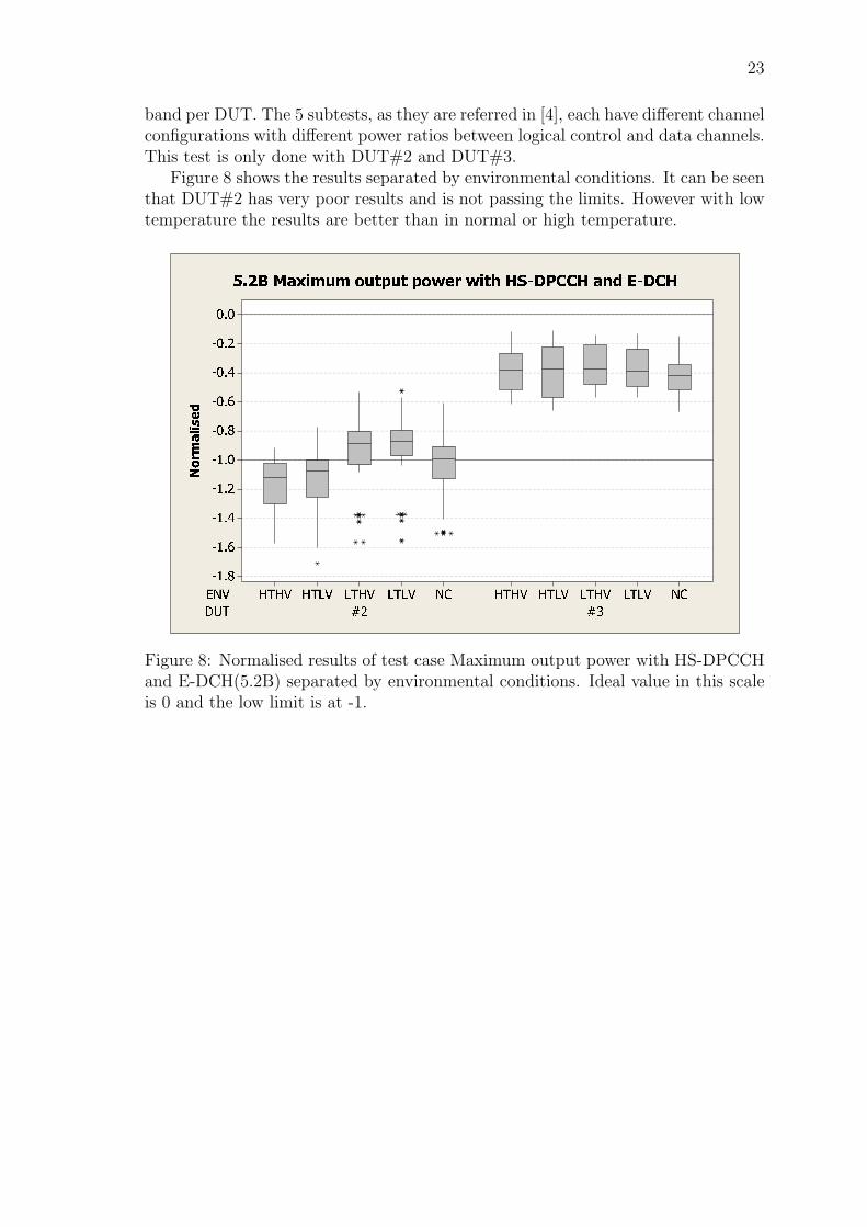
Test case 5.2B is consisted of 15 frequency/condition combinations. But, becausetest is performed as five different subtests, the amount of measurements is 75 per

23

band per DUT. The 5 subtests, as they are referred in [4], each have different channelconfigurations with different power ratios between logical control and data channels.This test is only done with DUT#2 and DUT#3.

Figure 8 shows the results separated by environmental conditions. It can be seenthat DUT#2 has very poor results and is not passing the limits. However with lowtemperature the results are better than in normal or high temperature.

Figure 8: Normalised results of test case Maximum output power with HS-DPCCHand E-DCH(5.2B) separated by environmental conditions. Ideal value in this scaleis 0 and the low limit is at -1.

24

Frequency Error(5.3)

The test is done in all environmental configurations using all three frequency chan-nels. This results in 45 measurements per DUT when three bands was tested. Theresults were divided by environmental conditions but that did not suggest any de-pendence of operating temperature or voltage. Therefore the most useful way tolook at the data is to only split it by DUT. The results are presented in figure 9.All medians are close to zero and the box heights are reasonable. DUT #3 has thesmallest variance.

Figure 9: Normalised results of test case Frequency error(5.3). Ideal value in thisscale is 0 and the test limits are at -1 and +1.

Open Loop Power Control(5.4.1)

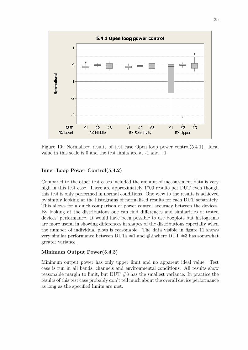
Included data consists of following combination of parameters: three bands, threechannels per band, three received power levels and five environmental conditions.The results of this test case show the biggest differences when separated by teststep, i.e. RX power level. The results are presented in figure 10. The differencebetween different DUTs is visible, as DUTs #1 and #2 have less variance over #3.The most obvious observation is however the fact that DUT#1 has problems in thetest step with highest RX power.

25

Figure 10: Normalised results of test case Open loop power control(5.4.1). Idealvalue in this scale is 0 and the test limits are at -1 and +1.

Inner Loop Power Control(5.4.2)

Compared to the other test cases included the amount of measurement data is veryhigh in this test case. There are approximately 1700 results per DUT even thoughthis test is only performed in normal conditions. One view to the results is achievedby simply looking at the histograms of normalised results for each DUT separately.This allows for a quick comparison of power control accuracy between the devices.By looking at the distributions one can find differences and similarities of testeddevices’ performance. It would have been possible to use boxplots but histogramsare more useful in showing differences in shapes of the distributions especially whenthe number of individual plots is reasonable. The data visible in figure 11 showsvery similar performance between DUTs #1 and #2 where DUT #3 has somewhatgreater variance.

Minimum Output Power(5.4.3)

Minimum output power has only upper limit and no apparent ideal value. Testcase is run in all bands, channels and environmental conditions. All results showreasonable margin to limit, but DUT #3 has the smallest variance. In practice theresults of this test case probably don’t tell much about the overall device performanceas long as the specified limits are met.

26

Figure 11: Histograms of normalised results of test case Inner loop power con-trol(5.4.2). Test limits are at x-axis values -1 and +1.

Transmit ON/OFF Time Mask(5.5.2)

The numerical results available from the used test system consist only of power levelmeasurements with TX on and off. The actual timing information is only availableas graphic presentations and cannot be therefore analysed with numerical methods.The results consist of three power measurements: one before transmission(TX off)one during transmission(TX on) and one after transmission period(TX off). Theseresults can be used as any other power level measurements taking the tolerancesinto consideration. The test is performed in normal and extreme conditions with allmeasurement channels. By looking at the actual results no conclusions can be madebecause the variations are so small compared to the margins.

Change of TCF(5.6)

The test case provides a single power ratio with DPDCH on/off. The test is per-formed in normal conditions with center channel only. Therefore the amount of datais very small. This data does not contribute much to overall performance evaluationsince all results are clear passes with reasonable margins.

Power Setting in Uplink Compressed Mode(5.7)

There are a total of 72 data points per each DUT in this test case. The test is onlydone in normal conditions but all three channels are tested. There are several teststeps with different power control patterns but the normalised values do not revealany differences between the DUTs.

27

Occupied Bandwidth(5.8)

Measurement of occupied bandwidth is performed in normal conditions using allthree measurement channels. The result is a figure in MHz. There are no significantvariations between the devices in this test case.

Spectrum Emission Mask(5.9)

Test case is performed in normal conditions with all three frequency channels and it issplit into several steps each covering different area of the spectrum. The results fromthese test cases are essentially spectra of the leaked power, but the test system alsoreports numerical values for each measurement interval. The covered spectrum isdivided into intervals because of their different limits and measurement bandwidths.The reported values are decibels scaled so that value zero is the limit and negativevalues represent power levels below this limit. Reported values represent the highestlevels inside each interval.

Figure 12 shows the boxplots of the results separated by DUT and frequencyoffset from the carrier. This grouping has been achieved by combining the results ofintervals with equal negative and positive offsets. There are differences between theDUTs and as the plots show DUT#3 has the greatest safe margin to the limit whenthe offset is small. When the distance from the carrier increases the measurementseven out so that all DUTs have similar performance. With the small offsets themargins to the limit are only under a decibel with DUTs #2 and #3 in the worstresults. Medians are between -10dB and -5dB. The shapes of the boxes indicatethat the number of values very close to the limit is small, as the median is closer tothe bottom of the box.

Spectrum Emission Mask with HS-DPCCH(5.9A)

The measurement methodology and metrics are similar to Spectrum emission mask.The amount of data is higher due to four subtests testing different uplink channelpower distributions. In boxplot of figure 13 the results are separated by measurementband offset and device. The results follow the trend of test case 5.9 because themargins are greater with larger offsets. But when looking at differences betweendevices the two test cases are not similar. The test with HS-DPCCH shows clearlysimilarities between DUTs #1 and #3 with small frequency offsets but with largeroffsets every DUT is different. DUT #2 seems to be the best performing device withthe smaller offsets. With the two biggest offsets DUT #1 has the largest margins.

28

Figure 12: Results of test case Spectrum emission mask(5.9) expressed as marginsto the test limit.

Figure 13: Results of test case Spectrum emission mask with HS-DPCCH(5.9A)expressed as margins to the test limit.

29

Spectrum Emission Mask with E-DCH(5.9B)

Like the HSDPA version above the HSUPA version of spectrum emission mask hasseveral subtests for different channel power allocations. The test is also done withthree channels and only in normal conditions. The results have again been separatedby the measurement band offset and device under test. Figure 14 shows the resultswhich are somewhat similar to test case 5.9A: With smaller offsets both DUTs arecloser to limit and DUT #2 seems to perform better in every case.

Figure 14: Results of test case Spectrum emission mask with E-DCH(5.9B) ex-pressed as margins to the test limit.

30

Adjacent Channel Leakage Power Ratio(5.10)

The test case is done in normal and extreme conditions using all three channels.Figure 15 shows the margins to the limit for the each measurement of the test caseseparated by the band, frequency offset of the measurement channel and deviceunder test. The units in the figure are decibels. Positive and negative adjacentchannels with same offsets have been grouped together because the similarity ofthe results and to keep number of boxes in one plot reasonable. Two major pointsare visible in the figure, the channel directly adjacent to the TX channel have thesmallest margins with every device and devices #1 and #2 have the worst resultsin band FDDII.

Figure 15: Results of test case Adjacent channel leakage ratio(5.10)expressed asmargins to the test limit.

Adjacent Channel Leakage Power Ratio with HS-DPCCH(5.10A)

This test case consisting of four subtests is done in normal and extreme conditionsusing all three channels. The results shown in figure 16 look similar to the resultsof 5.10 with one interesting detail: The DUT #2 problems with FDDII do not showin this test.

Adjacent Channel Leakage Power Ratio with E-DCH(5.10B)

The test case is also done in normal and extreme conditions using all three chan-nels. Figure 17 shows the results for ACLR with E-DCH as margins to the limit indecibels. The figure shows that especially with DUT #2 the most problematic areasare again the directly adjacent channels and in this case also band FDDI is showingsome problems in addition to FDDII.

31

Figure 16: Results of test case Adjacent channel leakage ratio with HS-DPCCH(5.10A) expressed as margins to the test limit.

Figure 17: Results of test case Adjacent channel leakage ratio with E-DCH(5.10B)expressed as margins to the test limit.

32

Spurious Emissions, TX(5.11)

The results of this case can be split into two categories based on the frequencyranges involved. The common ranges for all bands cover the whole spectrum from9kHz to 12.75GHz. In addition for some bands there are requirements for somespecific narrow ranges. The results of the common ranges for all the devices havereasonable margins to the limit and the data does not point out any interesting factsor potential risks. The comparison based on the band specific ranges is not possiblesince the amount of measurement data is small because the tests are different foreach band.

Transmit Intermodulation(5.12)

This test case provides 24 measurements per DUT consisting of eight intermodu-lation results for each band. The measurement is done with center channel only.Results are presented as boxplots in figure 18. The differences between DUTs aresmall in this test and there are no big differences between the intermodulation fre-quencies. This is not visible in the figure but was observed from the data.

Figure 18: Results of test case Transmit intermodulation(5.12). Values are marginsto the test limit in decibels.

33

Error Vector Magnitude(5.13.1)

The EVM results consist of measurements with all three channels in normal condi-tions using two transmit power levels. The results in figure 19 show that DUT#3has the highest measured values. There are some deviations between the bands butthose are much smaller than the differences between devices.

Figure 19: Normalised results of test case Error vector magnitude(5.13.1)

EVM and Phase Discontinuity with HS-DPCCH(5.13.1AA)

This test case has two types of results, EVM and phase discontinuity. Test is donewith three channels in normal conditions. The EVM values are measured at foursubframe positions and phase discontinuity figures are calculated between the firstand last pairs. The normalised results are presented in figures 20 and 21. Thistest case is only applicable release 6 onwards so DUT#1 is not tested. The mostinteresting part of the results is that DUT#2 has the biggest values in FDDII wherewith #3 the FDDI results stand out. For the phase discontinuity results of figure21 only thing that stands out is the larger range of variation of DUT#3.

34

Figure 20: Normalised EVM results of test case Error vector magnitude and phasediscontinuity(5.13.1AA)

Figure 21: Normalised phase discontinuity results of test case Error vector magni-tude and phase discontinuity(5.13.1AA)

35

UE Phase Discontinuity(5.13.3)

Test case results include phase discontinuity and EVM. The test case is methodolog-ically similar to the previous one(5.13.1AA) but is done without HS-DPCCH andphase discontinuity is calculated between two consecutive timeslots. All the phasediscontinuity measurements are between 0.25 and -0.25 on the normalised scale sothere is no risk seen in the data nor big differences between the DUTs. EVM valuesare higher with DUT #3 than with the two others as can be seen in in figure 22.This is very well in line with the results from EVM test case, 5.13.1.

Figure 22: Normalised EVM results of test case UE phase discontinuity(5.13.3)

PRACH Preamble Quality(5.13.4)

The test case is conducted with all three channels in all four environmental condi-tions. Frequency errors of 5.13.4 are plotted on figure 24 and EVM results in figure23. The results are separated by band. The frequency errors of DUT #3 are clearlythe smallest. The other two DUTs look almost identical in this figure. EVM resultsare interesting because also here DUT #1 and #2 have similar results: the bandVIII has the smallest EVM and bands I and II are almost equal. The frequenciesof the bands could be the explaining factor since both FDDI and FDDII uplink fre-quencies are around 1900MHz where FDDVIII is centered at 900MHz. For DUT #3the overall results are higher and there is not a clear difference between the bands.

36

Figure 23: Normalised EVM results of test case PRACH preamble quality(5.13.4)

Figure 24: Normalised frequency error results of test case PRACH preamble qual-ity(5.13.4)

37

Receiver Tests(6.2–6.8)

The measured bit error ratios for test cases 6.2 Reference sensitivity level, 6.3 Max-imum input level, 6.3A Maximum input level for HS-PDSCH reception, 6.4A Ad-jacent channel selectivity and 6.7 Intermodulation characteristics were all zero re-gardless of the DUT. This result shows that all the tested devices do perform wellin the receiver tests, but putting them in order or evaluating weak areas is simplynot possible. Analysing of a larger selection of devices should be done to find outif the results can be generalised. One option enabling the comparisons would be torun the test cases with tighter parameters than required.

Blocking(6.5) and spurious response(6.6) test cases were not included in theanalysis scope of this work. This is due the nature of the blocking test: A BERmeasurement is performed over 12000 times. Most of the measurements produce zeroBER and those that are something else usually count as exceptions to be measuredin test case 6.6. The number of these exceptions could be one starting point foranalysis but this test case does not suite the analysis methods used in rest of thetest cases in this thesis.

Test case for RX spurious emissions(6.8) does give some information about thesimilarity of the DUTs #1 and #2. They have larger variance of results and slightlysmaller margins than DUT #3. The results are presented as margins to the limit infigure 25 which only includes the common ranges and not the band specific ones.

Figure 25: Results of test case Spurious emissions(6.8) expressed as margins to testlimit.

38

6 Application of Analysis to Test Planning

Test planning is here selection of test cases to be included in a test round. This kindof planning is generally only needed for tests done for R&D purpose. The actualregulatory and organisational requirements define the necessary tests, so optimisingthose test sets in this way is not possible. When planning a test set the mostvaluable resource is time spent on a test system. Using every available test case isobviously the most thorough choice, but usually testing resources are limited. Thisleads to the need to limit the number of test cases in a test round. To use test timeeffectively it is important to know the duration of each individual test case. If atest case takes a long time to run and it provides little information, it should notbe prioritised over shorter tests providing more information.

The approach taken here is to use the measured and analysed data presentedin previous chapters as a basis for test planning. This is simply done so that if atest case shows differences between the tested devices it is selected to the test set.Test times of the individual test cases were considered during the selection. Thedurations of the test cases to be included were reasonable so there were no need torule tests out because of too long test time. It should be noted that the selected testcases might leave some critical tests out, based only on the fact that the test gavesimilar result for all the devices tested. That is why this set of test cases shouldonly be used as a starting point and the main focus of the test round should be oncomparing or tracking performance differences between device models or versions.This kind of comparison test set could be used when tracking performance of adevice during the design process or to find out the weak and strong areas of a newdesign compared to a known implementation.

A different approach for the receiver tests is also presented because using thestandard test method did not make comparisons possible as all the DUTs testedgave the same results. This is discussed in chapter 6.3.

6.1 Test Times

It is not possible directly influence the time it takes to perform individual test casesas the time is determined by a test system specific initialisation, call setup and thenthe measurement itself. Depending on the test case there may be multiple call setupsand releases during the test. Test times of the included test cases are presented intable 2. The times are gathered from the tests performed for the thesis and theyinclude the call setup and release. The durations have small variations between runseven with the same DUT but the values listed should be a good estimate as theyare based on several iterations of the test cases. Total duration of each test case inthe table is the amount of time required for the test case to be run in one frequencyband including all the channel and environmental condition combinations.

The total time of a test set can be influenced by the selection of test cases andparameters which include frequency band, channel, voltage and temperature. Thevoltage and temperature are together addressed in test specification as environ-mental conditions and separated as normal and extreme conditions. The normal

39

conditions include only the normal voltage and temperature so it means one run ofa test case. The extreme conditions include both high and low voltage and highand low temperature which gives a total of four combinations. According to thespecification[4] all the test cases are required to be performed in normal conditionsand in addition a subset of them is to be performed in extreme conditions. Theduration required for the temperature adjustment and stabilisation is not includedin the test times table. Stabilisation is only required when DUT is tested in extremetemperatures as the normal conditions allow moderate variations in room temper-ature. Typical duration for the stabilisation is 45 minutes. By properly arrangingthe test cases the stabilisation is needed only twice during a full test set.

6.2 Test Set Recommendation

Based on the results presented in chapter 5 of this thesis the following test cases arerecommended to be used as a starting point when creating a test set for comparingtwo or more devices. The durations are given for one band including all channelsand environmental conditions excluding the set-up and stabilisation times requiredfor temperature changes. Test durations can change according to UE release andfeatures because of the applicability of test cases. The times given are for a release6 UE supporting HSUPA which is typical for a present-day UE. In addition todescriptions below the recommended test cases are also presented in table 2.

The total duration of this test set is about 5.5 hours not including the stabil-isations etc. The test time could be considerably shortened by running the testsonly in normal conditions. This leaves out all temperature and voltage dependentphenomena and it should be carefully considered what effects this might have onthe reliability of the conclusions. Another approach would be doing a study of therelations of the results of test cases and the environmental parameters to find outif reasonable test coverage could be achieved by selecting only part of the combina-tions.

Maximum output power

The test cases 5.2–5.2B cover the maximum output power requirements so that 5.2is applicable for all devices and additionally one of 5.2A, 5.2AA or 5.2B is requireddepending on the release version of the UE. For modern high-end devices this meanstest cases 5.2 and 5.2B. The total duration of the test cases is, derived from table 2,49.5 minutes. These test cases are recommended because they can reveal differencesin the performance of the transmitter at the high end of the dynamic range.

Spectrum emission mask

The test cases 5.9–5.9B describe the requirements for spectrum emission mask. Therequirement for release 6 UE is that all three test cases are run. The total durationof these is 15.5 minutes. The results of these test cases revealed clear differencesbetween the DUTs.

Adjacent channel leakage ratio

40

Adjacent channel leakage ratio requirements are spread to test cases 5.10, 5.10A and5.10B. They are included in the recommended test set because the results suggestpossible risks due to some failing results. These test cases also showed differentresults between DUTs. The correlation between the three test cases seem to bequite low and therefore they all are included. The total duration is 2 hours 23minutes. The seemingly long duration is a result of testing in extreme conditions.The effect of the condition parameters should be studied to find out if it is possibleto shorten test time by selecting only part of the test cases and conditions.

Error vector magnitude and phase discontinuity

Error vector magnitude and phase discontinuity are measured in three test cases forrelease 6 UE: 5.13.1, 5.13.1AA and 5.13.3. The test cases are a good measure oftransmitter properties and the data suggests some differences between the DUTs.The total time for the three test cases is 29 minutes.

PRACH preamble quality

The test case 5.13.4 shows some differences between the DUTs. Visually comparingthe results of this test case to 5.13.1 EVM shows some correlation and it should beconsidered if either one should be left out from the test set to reduce the duration.However, this test case is included because it fills the criteria of showing differencesbetween the devices. Test time is about 1.5 hours.

6.3 Iterative Method for Receiver Tests

From the test results it can be seen that if these devices should be compared byreceiver performance, the test cases should be run using conditions that are harderfor the UE than is required in the specifications. A natural way to achieve this is touse iterative testing method where the worst test condition in which the UE passesthe test limits is searched. The Anritsu test system used allows this iteration to bedone in all required test cases. The iteration method is similar in all the test cases.A parameter is selected as the iteration variable and it is changed by the step sizeafter each iteration. The direction of change is determined by BER measurementresult so that when the BER is below the limit the conditions are toughened andvice versa. The used step size for level changes and the target BER can be chosenby the user. Also the minimum and maximum values of the variable are selectable.This is required in order to avoid levels that could be dangerous to the device undertest and to limit the amount of iterations and hence test time. [22]

The method was tested to verify the functionality of the iterative method forthe selected test cases and to test if there were any limitations by the test system.The test cases were run with a new DUT not used in the original test rounds so theresults are not comparable. Only band FDDI in normal conditions was tested usingcenter channel.

For test case 6.2 Reference sensitivity level the varied parameter is downlinktransmission power. The step size used was 0.5dB and maximum span was set to20dB. The requirement for this test case is -106.0dBm and the result was -109.5dBm.

41

For test case 6.3 Maximum input power the step size for input power was 1dB andthe span was set to 20dB. This turned out to be too big value since the system didnot support larger value than -20.0dBm/3.84MHz where system limit was reported.Requirement was -25.7dBm/3.84MHz.

Test case 6.4A Adjacent channel selectivity(Rel. 5 and later) includes measure-ments with interferers on both upper(+5MHz) and lower(-5MHz) adjacent channelsseparately. The test is also done with two power levels and thus separated to case1(lower level) and case 2(higher level). Case 2 is done with 27dB greater downlinkand interferer levels than case 1 when the specified levels are used. The iteratedvariable in this case is the interferer level. Span was set to 20dB and step size to1dB. The results for case 1 were -42dBm for both upper and lower adjacent channelswhere the limit was -52dBm. For case 2 the results were -21dBm and -22dBm forupper and lower adjacent channels respectively the limit being -25dBm.

Test case 6.7 Intermodulation characteristics includes two interfering signals:the WCDMA simulating noise signal and a sinusoidal signal. Both signals have thesame level which is specified at -46dBm. Two frequency combinations are tested:The first case includes sinusoidal interferer at -10MHz from the carrier with thesimulated WCDMA signal lying at -20MHz. The second combination is the samebut with positive offsets. The possible intermodulation results should appear on thecarrier frequency. The iteration is performed altering the level of the two interferersin synchronous manner with step size of 1dB. Results were -38dBm for interferersbelow the carrier frequency and -39dBm for the interferers above the carrier.

Using this one DUT the method was proven useful for test cases 6.2, 6.4A and6.7. Test case 6.3 did not give any additional information since test system limit wasreached. A larger study with more devices should be made to find out if the resultsare useful in comparisons between devices. As emphasised before test time shouldbe always considered when suggesting changes in testing. The effect on test timesis of course dependent of the number of iterations required but as one measurementtakes a second the real impact is reasonably small. Of the included tests the greatestdifference was observed with test case 6.2 where the time was increased to 1 minute26 seconds from 31 seconds. Relationally this is a great change but as all the testsin question are originally short using this method would not add the test timesignificantly.

42

Table 2: Test durations of the test cases discussed in this thesis. Test case numberingfollows [4]. Measurement conditions and channels are also presented. Total durationincludes all the channels and environment combinations required for each test. Testcases marked with ’X’ are included in the recommended test set discussed in chapter6.2

TC n.o. Duration Conditions Channels Total Rec.5.2 00:00:18 NC+EC L,M,H 00:04:30 X5.2A 00:01:15 NC+EC L,M,H 00:28:45 X5.2AA 00:02:00 NC+EC L,M,H 00:30:00 X5.2B 00:03:00 NC+EC L,M,H 00:45:00 X5.3 00:00:21 NC+EC+V L,M,H 00:06:185.4.1 00:03:16 NC+EC L,M,H 00:49:005.4.2 00:01:42 NC M 00:01:425.4.3 00:00:20 NC+EC L,M,H 00:05:005.4.4 00:01:21 NC M 00:01:215.5.1 part of 5.5.2 NC+EC L,M,H part of 5.5.25.5.2 00:01:59 NC+EC L,M,H 00:29:455.6 00:00:27 NC M 00:00:275.7 00:00:58 NC M 00:00:585.7A 00:03:47 NC M 00:03:475.8 00:00:16 NC L,M,H 00:00:485.9 00:00:21 NC L,M,H 00:01:03 X5.9A 00:01:00 NC L,M,H 00:03:00 X5.9B 00:03:50 NC L,M,H 00:11:30 X5.10 00:00:25 NC+EC L,M,H 00:06:15 X5.10A 00:01:16 NC+EC L,M,H 00:19:00 X5.10B 00:07:50 NC+EC L,M,H 01:57:30 X5.11 00:03:09 NC L,M,H 00:09:275.12 00:00:36 NC M 00:00:365.13.1 00:00:35 NC L,M,H 00:01:45 X5.13.1A 00:01:22 NC L,M,H 00:04:06 X5.13.1AA 00:02:59 NC L,M,H 00:08:57 X5.13.3 00:18:39 NC M 00:18:39 X5.13.4 00:05:53 NC+EC L,M,H 01:28:15 X6.2 00:00:31 NC+EC L,M,H 00:07:456.3 00:00:51 NC M 00:00:516.3A 00:00:30 NC M 00:00:306.4A 00:01:30 NC M 00:01:306.5 08:20:00 NC M 08:20:006.6 00:00:13 NC M 00:00:136.7 00:00:48 NC M 00:00:486.8 00:01:53 NC L,M,H 00:05:39

43

7 Conclusions

This thesis concentrates on result analysis of 3G RF conformance tests. Character-istic properties of WCDMA and UMTS are discussed in chapter 2. The test casesincluded in the scope are introduced in Chapter 3. In chapter 4 a normalisationscheme for presenting the results in a common scale and a graphical presentation,boxplot, for visualising the data are presented. The measurement equipment andthe analysis results are discussed in chapter 5. Chapter 6 is used to propose a set oftest cases that are shown to provide differences between devices. The chapter alsoincludes a description of an alternative test method to gain additional value fromreceiver tests.

The visual analysis using boxplots was shown to give additional value out ofconformance test results. Applying normalisation to the data and then representingthe results as boxplots enables comparisons between devices. The use of this kindof analysis could save some valuable test time in the product development becausethe analysis enables discovering the performance differences between device models.The visualisations enable also observing the margins to the test limits, which canbe used to identify risky areas between or inside test cases. An example of this isvisible in figures 12 to 14 where the smaller offsets are clearly having the smallestmargins.

In order to gain the best value out of the boxplots, the selection of parameters tobe used to separate the boxes must be done carefully. Currently there are no betterways of doing this than by relying on the previously gathered information or by trialand error. The optimal result is probably obtained by a combination of these two.

By using the analysis results it was made possible to form a recommended testset to be used in benchmarking devices. This set consists of the test cases that wereshown to provide different results between two or more of the tested devices. Theselected test cases are marked with ’X’ in table 2 and the reasoning behind each testis explained in chapter 6.2. The applied method does include a risk of leaving outuseful test cases and probably use of larger set of different types of devices wouldbe a good option to lower that risk.

The selection of environmental conditions and test cases together for research& development tests should be addressed in future studies. By selecting the testcases to be run only in some environmental conditions the total test times could beoptimised. One approach for doing this would be to analyse a large set of devicesto find out what conditions are the most difficult for each test case and then onlytest in those conditions.

The results of receiver bit error ratio measurements were identical for all thetested devices. All the tests resulted in zero BER. This gave a reason to studythe possibilities of the used test system and as a result they were later run with adifferent test mode to test the functionality in practice and gain information abouttest duration. This iterative method was found out to be useful with some testcases but was only tested with one DUT so a comparative analysis between differentdevices was not done. This should be evaluated and studied more before this modeof testing can be recommended to be taken in systematical use.

44

It was found out that generating the graphics from test system output files in away it was done is not feasible for everyday use. The time consumed by doing manualmechanical work is simply too long. However, the observations made in the thesissupport the idea of developing tools to help performing the analysis tasks. Withproper tools the analysis could be used in daily work as a value-adding reportingformat. Starting the development of such tools from the test cases listed in therecommended test set would probably be the best approach and give the most addedvalue.

45

References

[1] Official Journal of the European Communities, Directive 1999/5/EC of theEuropean Parliament and of the Council of 9 March 1999 on radio equipmentand telecommunications terminal equipment and the mutual recognition of theirconformity

[2] Global Certification Forum, Internet page, Accessed 2010-03-25, http://www.globalcertificationforum.org/WebSite/public/home_public.aspx

[3] PCS Type Certification Review Board, Internet page, Accessed 2010-03-25,http://www.ptcrb.com/index.cfm?tab=Home

[4] 3rd Generation Partnership Project 2008, User Equipment (UE) conformancespecification; Radio transmission and reception (FDD); Part 1: Conformancespecification, 3GPP TS 34.121-1, version 8.5.0, http://www.3gpp.org/ftp/

Specs/archive/34_series/34.121-1/34121-1-850.zip

[5] ETSI 2007, Electromagnetic compatibility and Radio spectrum Matters (ERM);Base Stations (BS), Repeaters and User Equipment (UE) for IMT-2000 Third-Generation cellular networks; Part 2: Harmonized EN for IMT-2000, CDMADirect Spread (UTRA FDD) (UE) covering essential requirements of article 3.2of the R&TTE Directive, ETSI EN 301 908-2, version 3.2.1

[6] China Daily, China Mobile to spend 58.8 bn yuan in 3G network, Internet page,Updated 2009-01-10, Accessed 2010-03-21, http://www.chinadaily.com.cn/china/2009-01/10/content_7385184.htm

[7] Holma, H., Toskala, A. (edited) WCDMA for UMTS: Radio Access for ThirdGeneration Mobile Communications 3rd edition, John Wiley & Sons, GreatBritain, 2004

[8] Reinhold, K.,Mellein, H. UMTS Introduction and Measurement, Ro-hde&Schwarz GmbH&Co. KG, Germany, 2004

[9] Laiho, J., Wacker, A., Novosad, T. (edited) Radio Network Planning and Op-timisation for UMTS; Second Edition, John Wiley & Sons, 2006

[10] 3rd Generation Partnership Project 2009, Technical Specification Group Ra-dio Access Network; User Equipment (UE) radio transmission and reception(FDD); 3GPP TS 25.101, version 8.5.1, http://www.3gpp.org/ftp/Specs/

archive/25_series/25.101/25101-851.zip

[11] Holma, H., Toskala, A. (edited) HSDPA/HSUPA for UMTS: High Speed RadioAccess for Mobile Communications, John Wiley & Sons, 2006

[12] 3rd Generation Partnership Project, 3GPP Homepage: releases, Internet page,Accessed 18.03.2009, http://www.3gpp.org/releases

46

[13] Lempiainen, Tero, Comparison of Two Mobile Devices in Terms of WCDMALayer 1 Performance, Special assignment for course S-88.3155 Signal Processing,2008

[14] 3rd Generation Partnership Project 2009, User Equipment (UE) / Mobile Sta-tion (MS) Over The Air (OTA) antenna performance; Conformance testing,3GPP TS 34.114, version 8.3.0, http://www.3gpp.org/ftp/Specs/archive/34_series/34.114/34114-830.zip

[15] Tanner, R.,Woodward, J. (edited) WCDMA - Requirements and Practical De-sign, John Wiley & Sons, 2004

[16] Loke, A., Fazal, A. Direct Conversion Radio for Digital Mobile Phones–DesignIssues, Status and Trends IEEE Transactions on Microwave Theory and Tech-niques, vol. 50, no. 11, November 2002

[17] TestAnalysis wiki, Nokia Intranet, Accessed 2009-12-21

[18] 3rd Generation Partnership Project 2008, Technical Specification Group RadioAccess Network; Terminal logical test interface; Special conformance testingfunctions; 3GPP TS 34.109, version 8.0.0, http://www.3gpp.org/ftp/Specs/archive/34_series/34.109/34109-800.zip

[19] Tukey, John W, Exploratory Data Analysis, Addison-Wesley, Reading, MA,1977

[20] 3rd Generation Partnership Project 2009, Technical Specification Group RadioAccess Network; Common test environments for User Equipment (UE); Confor-mance testing(Release 8); 3GPP TS 34.108, version 8.5.0, http://www.3gpp.org/ftp/Specs/archive/34_series/34.108/34108-850.zip

[21] Anritsu ME7873F TRx/Performance Test System product information, Inter-net document, Accessed 2009-08-05, http://www.anritsu.co.kr/product/

download_files/ME7873F_74F_EL1400-1196839034.pdf

[22] ME7873F W-CDMA TRX/Performance Test System / ME7874F W-CDMARRM Test System Product Brochure, Anritsu Corporation, Internet doc-ument, Accessed 2010-02-03, http://www.anritsu.co.uk/files/ME7873F_

74F_E1700.pdf