1

CSCI 350Ch. 7 – Scheduling

Mark Redekopp

Michael Shindler & Ramesh Govindan

2

Overview

• Which thread should be selected to run on the processor(s) to yield good performance?

• Does it even matter?

– Does the common case of low CPU utilization mean scheduling doesn't matter since the CPU is free more often that it is needed

– Yes in certain circumstances!• Scheduling matters at high utilization (bursts of heavy

usage)

• Google and Amazon estimate they lose approximately 5-10% of their customers if their response time increases by as little as 100 ms (OS:PP 2nd Ed., p. 314)

– When do you care about scheduling at the grocery store checkout…at 6 a.m. or 5 p.m.

• Many OS scheduling concepts are applicable in other applications: web servers, network routing, etc.

“The Case for Energy-Proportional

Computing”, Luiz André Barroso, Urs Hölzle,

IEEE Computer, vol. 40 (2007).

3

Choices

• Under heavy utilization important choices must be made

– Should you turn away some users so others experience reasonable response times?

• If so, which users should you turn away?

– How much benefit would additional resources have?• In most cloud providers, you can dynamically reprovision (i.e. spin

up more servers on the fly)

– Can you predict the degradation if the number of requests doubles?

• Might it be worth it to switch scheduling strategies on the fly?

– Do insights into the context and kind of requests matter?• Denial-of-service attack?

4

Terminology

• Task (job): A user request

• Workload: The mix (type) of tasks and their arrival time– Compute bound: Processor resources impose a bound on performance

– I/O bound: I/O delay imposes a bound on performance

• Response Time (delay): Time from when the user submits the task until the user experiences its completion

• Throughput: Rate at which tasks are completed

• Predictability: Low variance in response times of repeated requests

• Scheduling overhead: The time to switch from one task to the next

• Fairness: Equality in the number and timeliness of resources allocated to a task

• Starvation: Lack of progress of a task due to resources given to another (higher-priority) task

5

Uniprocessors

• Let's start with a simple uniprocessor system assuming:

– Preemptive multitasking: OS can switch thread at its discretion

– Work-conserving: If a task is ready, the OS will not leave the processor idle (in preparation for some future event)

• Possible scheduling algorithms:

– FIFO (FCFS = First come first serve)

– SJF (Shortest Job First)

– Time-sliced Round-robin

6

FIFO

• Under FIFO, the job that arrives first runs to completion

• Avoids overhead increasing throughput

– Optimal since least possible overhead of context switching

• Maintains a simple queue

• Is it fair?

– In one sense, yes.

– But worst-case response times may result if long running job arrives before the short ones (grocery store)

• If jobs are all of equal size, then it can be optimal

40

5

T0

T1 arrives

T2-5 arrives

T1

T2

5

5

5

T3

T4

T5

Workload 1 (Avg. Resp. time =

(40+45+50+55+60)/5 = 50

5

5

T0

T1-5 arrives

T1

T2

5

5

5

T3

T4

T5

Workload 2 (Avg. Resp. time =

(5 + 10 + 15 + 20 + 25)/5 = 15

7

Shortest Job First (SJF)

• Requires prior knowledge of length of task

– Impossible?

• Uses some form of priority queue to determine next job to run (i.e. shortest duration)

• It is preemptive!– If a shorter job arrives during execution of

another, SJF will context switch and run it

– Thus, it is actually Shortest Remaining Job First

• Provides optimal average response time

• Provides worst-case variance in response time

– A shorter job can always come in and "cut" in front of a waiting task (i.e. starvation)

• Can you game the SJF system if you are a long task?

40

5

T0

T1 arrives

T2-5 arrives

T1

T2

5

5

5

T3

T4

T5

Workload 1 (Avg. Resp. time =

(5+10+15+20+60)/5 = 22

8

5

T0

T1 arrives

T2-5 arrives

T1

T2

5

5

5

T3

T4

T5

5T6

40

32

T6 arrives

8

Round Robin

• Execute each task for a given time quantum and then preempt

– No more starvation

• How to choose the time quantum– To short, overhead goes up due to excessive

context switches (also consider caching effects when switching often)

– To long, response times suffer (see bottom graphic)

• FIFO and SJF can be thought of as special cases of RR

– FIFO (RR with time quantum = inf.)

– SJF (approx. RR with time quantum = epsilon)• Assume 0 overhead switch, set epsilon to 1 instruc.

• Within a factor of n if n schedulable tasks

• Predictable though higher response times

– Why?

5

T0

T1 arrives

T2-5 arrives

T1

T2

5

5

5

T3

T4

T5

Time quantum = 5 ms

Avg. Resp. time = (60+10+15+20+25)/5 = 26

5 35

5

T0

T1

T2

5

5

5

T3

T4

T5

Time quantum = 20 ms

Avg. Resp. time = (60+25+30+35+40)/5 = 38

20 20

9

Round-Robin On Equal Size Tasks

• Poor effect on response time but low variability

– Consider a server streaming multiple videos

10

Mixed Workloads• All examples thus far have been compute bound (i.e. tasks are able to use the

processor for their entire time quantum)

• Under mixed workloads (some I/O and some compute bound tasks) issues of fairness arise even in round-robin

• Consider an I/O bound process in the presence of two other compute bound tasks (compute for full 100 ms of their time quanta)

– I/O process starts a 10 ms disk read, compute briefly (1 ms) and then blocks, yielding its time slice

– Recall, we assume work-conserving so we won't just idle waiting for the disk to finish

11

Max-Min Fairness

• Idea: Give priority to processes that aren't using their fair share of resources

• Note: max-min is not necessarily on top of round-robin

• Max-min: Maximize (responsiveness to) the minimum request

– If any task needs less than its fair share, give the smallest (minimum) its full (maximum) request (i.e. schedule)

– Split the remaining time among the N-1 other requests using the above technique (i.e. recursively)

– If all tasks need more than an equal share, split evenly and round-robin

• Max-min Approximation: Give priority to task that has received the least processor time

• Originally used/proposed for network link utilization (a short download in the face of a long one)

Consider 4 programs: • P1 wants 10% of processor's time• P2 wants 20% of processor's time• P3 and P4 each would want 50% of the

processor's time on their own.

Fair share would be 25% each

1. Since P1 is minimum and wants < 25% we'll always schedule it (maximize it) when it is available in the ready list

2. We now have 90% of the processor we can split 3 ways (i.e. fair share is now 30%)

3. We recurse and give P2 it's 20% (scheduling it when it's available but P1 isn't).

4. We split the remaining 70% between P3 and P4 (35% each) using round-robin as needed

Example

12

MLFQ

• Multi-Level Feedback Queue

– Implemented by most modern OSs

• Unix, Linux, Windows (w/ some variation), Mac OSX?

– Like round-robin but with multiple queues of different priority

• Goals: Reasonable compromise to achieve:

– Response time, Low overhead, No-starvation, fairness, de-prioritize background tasks

– A compromise to achieve similar results as max-min fairness

13

MLFQ Rules• Multiple queues with different priorities

– Higher priority queues => Smaller time quantum

– Lower priority queues => Larger time quantum

• Rules:

– Rule 1: Higher priority always runs, preempting lower priority tasks

– Rule 2: RR within same priority

– Rule 3: All threads start at highest priority

– Rule 4a: If thread uses up quantum, reduce priority (i.e. move to lower priority queue)

– Rule 4b: If thread gives up processor, stays at same level• Alternative: once total quantum is taken up, demote

• Shorter tasks finish quickly; I/O bound tasks get priority

– Rule 5: After some time S, move threads back to highest priority

• Avoids starvation

• Uses recent past to predict future

Key Idea: We can't predict the length of a job so assume it is short and then demote it the longer it runs.

14

MLFQ Examples

Refer to the source of these images for a nice writeup:

http://pages.cs.wisc.edu/~remzi/OSTEP/cpu-sched-mlfq.pdf

• Example 1: A long running job

– Starts at high priority and migrates to lower priority with longer time slices

• Example 2: A short job arrives during execution of the long running job

– Preempts long job and may complete before it reaches Q0

15

MLFQ Examples

Refer to the source of these images for a nice writeup:

http://pages.cs.wisc.edu/~remzi/OSTEP/cpu-sched-mlfq.pdf

• Example 3: I/O bound job and compute bound job

– I/O bound job preempts compute-bound job

– Any issue with this scheme?

• Example 4: Intermittent priority boosts to avoid starvation

– Helps if a compute-bound job transitions to become interactive (I/O-bound)

16

MLFQ Examples

Refer to the source of these images for a nice writeup:

http://pages.cs.wisc.edu/~remzi/OSTEP/cpu-sched-mlfq.pdf

• Example 5: Change Rule 4 to avoid gaming the system

– Consider a program that "sleeps" for 1 ms after computing for 99 ms

– Rule 4b: If thread gives up processor, stays at same level

– New Rule 4: Once total quantum is taken up (over several context switches), demote

17

MULTIPROCESSOR PERFORMANCE

Effects of caching, false sharing, etc.

18

Cache Coherency• Most multi-core processors are shared memory systems where

each processor has its own cache

• Problem: Multiple cached copies of same memory block– Each processor can get their own copy, change it, and perform

calculations on their own different values…INCOHERENT!

• Solution: Snoopy caches…

P1

$

P2

$

M

P1

$

P2

$

M

P1

$

P2

$

M

P1

$

P2

$

M

P1

$

P2

$

M

1 2 3 4aP1 Reads X

Block X

P2 Reads X P1 Writes X

if P2 Reads X it

will be using a

“stale” value of X 4b

if P2 Writes X we

now have two

versions. How do we

reconcile them?

Example of incoherence

19

Snoopy or Snoopy

20

Solving Cache Coherency• If no writes, multiple copies are fine

• Two options: When a block is modified– Go out and update everyone else’s copy

– Invalidate all other sharers and make them come back to you to get a fresh copy

• “Snooping” caches using invalidation policy is most common– Caches monitor activity on the bus looking for invalidation messages

– If another cache needs a block you have the latest version of, forward it to mem & others

P1

$

P2

$

M

P1

$

P2

$

M

P1

$

P2

$

M

P1

$

P2

$

M

1 2 3P1 & P2 Reads X

P1 wants to writes X,

so it first sends

“invalidation” over

the bus for all sharers

Now P1 can safely

write X 4

if P2 attempts to

read/write x, it will

miss, & request the

block over the bus

Coherency using “snooping” & invalidation

Invalidate

block X if

you have

it

Block X

5

P1

$

P2

$

M

P1 forwards data to

to P2 and memory

at same time

21

SpinLocks• Consider a spinlock held by a thread on

P3 (not shown) for a "long time" while thread 1 and 2 (on P1 and P2) try to acquire the lock

• Continuous invalidation of each other reduces access to the bus for others (especially P3 when it tries to release)

P1

$

P2

$

M

P1

$

P2

$

M

P1

$

P2

$

M

1 2 3

P1 wins bus and

performs

atomic_exchange,

writing BUSY (again)

P2 now wins bus and

"invalidates" P1's

version and writes

BUSY

P1 now wins bus,

invalidates P2 and

writes BUSY

again

Invalidate

block

l->val

void acquire(lock* l){

int val = BUSY;while( atomic_swap(val, l->val)

== FREE);}

Thread1

Thread2

P1

$

P2

$

M

4

P2 now wins bus and

"invalidates" P1's

version and writes

BUSY

Invalidate

block

…

P3

$

I wish I could get the bus!

22

False Sharing

• Thread-independent (i.e. non-shared) variables allocated on the same cache line

• Can cause a large performance degradation due to cache coherence (invalidates, etc.)

int x = 0;

int y = 0;

void t1() {

for(int x=ITERS; x > 0; x--);

y = 1;

}

void t2() {

while( y == 0);

printf(“Y was set to 1\n”);

}

T1

(Wr. X)

$

T2

(Rd. Y)

$

XCache Line Y

E I

T1

(Wr. X)

$

T2

(Rd. Y)

$S S

YCache Line

XCache Line

int x = 0;

int y __attribute__ ((aligned (64))) = 0;

…

False Sharing Example

One solution: Alignment

23

Is Cache Coherency = Atomicity?

• No, cache coherence only serializes writes and does not serialize entire read-modify-write sequences– Coherence simply ensures two processors don’t read two different

values of the same memory location

• Consider our sum example ( sum = sum + local_sum; )

P1

$

P2

$

M

P1

$

P2

$

M

P1

$

P2

$

M

1 2 3P1 & P2 both read sum P1 Writes new sum

invalidating P2

if P2 Writes X it will get updated line from P1,

but immediately overwrite it (not required to re-

read anything if not using locks, etc.)

24

MULTIPROCESSOR SCHEDULING

25

Typical Multicore Organization

• How do scheduling choices change when we have multiple processors that can be scheduled at the same time?

L1 $

Main Memory

P

Shared L2

Cache

Interconnect (On-Chip Network)

L1 $

P

L1 $

P

L1 $

PThis can be a shared bus or a

more complex switched network

Chip Multi-

Processor

26

Scheduler Data Structure Issues

• Allow processor affinity (i.e. which processor a thread is schedule on) for threads

– Warm caches vs. cold caches

• Single task queue (or MLFQ) or one for each processor

– Single queue suffers from

• Locking contention

• Cache coherence

P1

$

P2

$

M

If a thread is scheduled on one

core, context switched, and then

scheduled again on another core,

data may need to migrate. This

reduces performance.

P1

$

P2

$

M

MLFQ

Cached copies of the MLFQ data

structure must be kept coherent as

processors modify it.

27

Scheduler Data Structure Solutions

• Each processor can maintain its own queue, reducing lock contention and cache coherence performance penalties– Threads essentially stay "pinned" to a

certain processor

• Rebalancing across processor scheduling queues can be done only when it is "worth" it– i.e. When the benefit of being able to

schedule a thread on a different processor outweighs the cost of the locking and caching penalties (both for the scheduler queue and thread data)

P1

$

P2

$

M

MLFQ

Separate scheduling queues avoids

costly coherence. Migrate threads

(e.g. T1) only when the overhead is

outweighed by the rebalancing.

T1

28

Oblivious Thread Scheduling

• Consider a single program written to optimize performance by breaking work into many parallel threads

• Knowing the structure of a parallel program can be crucial to scheduling those threads in such a way as to achieve optimal performance

• If the thread scheduler is oblivious to the nature of the parallel program, performance can be severely impaired

– The next slide(s) show a few examples

29

Oblivious Scheduling Pitfalls

• Basic problem: Scheduler may treat all threads equally (i.e. many threads from many processes)

– By not knowing which threads come from what processes or that thread's role in the overall program, performance may suffer

• Various parallel program architectures may exhibit poor performance if threads from the program are improperly scheduled

– Bulk Synchronous Parallel (BSP): All threads compute, wait for others to finish computing, then exchange data for the next computation period

• Since threads must wait for all others, delaying a single thread may force all others to wait

– Staged (Producer/Consumer): Each thread performs one part of the work on an overall task.

• Delaying one can mean others don't have enough useful work

Stage

1

Stage

2

Stage

3

Bulk Synchronous Parallel

Staged

(Producer/Consumer)

30

More Pitfalls

• Various parallel program architectures may exhibit poor performance if improperly scheduled

– Critical path: Sometimes certain tasks (threads) are on the critical path of finishing the overall job while others have more slack on their deadlines

• If the critical path threads don't get scheduled the overall job performance will suffer

– Preemption of a lock holder

• Lock holder is context-switched thus holding off other threads from the program T1

T2 T3

Critical Path

Time

31

Gang Scheduling

• Gang Scheduling attempts to schedule (all of) the threads from one program on the processors at the same time

Prog. A

Proc1 Proc2 Proc3 Proc4

T1-A T2-A T3-A

T4-A X X

T1-A T2-A T3-A

T4-A X X

Assume 1 Progs (PA) with 4 threads and two

unrelated background threads

Bgrd. D Bgrd. E

Proc1 Proc2 Proc3 Proc4

T1-A T2-A T3-A T4-A

T1-A T2-A T3-A T4-A

T1-A T2-A

T3-A T4-A

Assume a BSP style program. T1-T3 can't run

again until T4 does.

Gang Scheduling may allow more progress in

the same time window.

32

Law of Diminishing Returns

• If a project would take 12 hours alone, does working in a group of 2 mean it will take 6 hours?

• Likely not. Communication adds overhead.– And a team of 4 will almost

certainly take much longer than 3 hours

• Many parallel programs do not continue to give linear speedup gains as you add more and more processors

Sp

ee

du

p (

Tim

es

Fa

ste

r vs

. 1

pro

c.)

Number of processors

Perfectly Parallel

Diminishing

Returns

Limited Parallelism

OS:PP 2nd Ed. Fig 7.12

33

Revisiting Gang Scheduling

• Just because we have 4 processors doesn't mean we should use 4 threads for a given program.

• Space sharing indicates multiple programs share the physical processors by using different subsets

• This is in contrast to time sharing where all processors are used for one program and then is swapped at the next time quantum

• We might achieve better throughput (not response time) for both Prog. A and Prog. B by only using 2 threads

– Notice here we don't need to context switch!

Prog. A

Assume 2 Progs (PA-PB) each with 4 threads

Prog. B

Proc1 Proc2 Proc3 Proc4

T1-A T2-A T3-A T4-A

T1-B T2-B T3-B T4-B

T1-A T2-A T3-A T4-A

T1-B T2-B T3-B T4-B

Proc1 Proc2 Proc3 Proc4

T1-A T2-A T1-B T2-B

T1-A T2-A T1-B T2-B

T1-A T2-A T1-B T2-B

T1-A T2-A T1-B T2-B

Time Sharing

Space Sharing

34

ENERGY-AWARE SCHEDULING

35

Energy vs. Performance Tradeoffs

• Modern HW systems can trade performance for power consumption (i.e. energy)

– Increase performance (rate of instruction execution) by consuming more power

– Heterogeneous cores (some high-performance high power cores and some low-performance low power cores)

– Powering on or off cores and I/O devices

36

Energy Policies & Scheduling

• On battery powered devices (laptops and phones) user's can often select an energy policy

– Lower performance and greater battery life

– Better performance and lower battery life

– Or a blend!

• To achieve this blend the scheduler needs to be involved

– Should I schedule this thread on the high performance, high power core?

– Would allowing threads from this program to get all the resources for a few time slices allow the some I/O device to be powered down temporarily?

37

Basic Approach

• If the lower performance is below human perception:

– Then lower performance and save energy

• If the lower performance is above human perception:

– Then optimize for performance so the user doesn't notice any difference

• Long-running and background tasks

– Try to achieve balance taking into account the available energy (i.e. battery level)

38

REAL-TIME SCHEDULING

39

Real-Time Constraints

• Hard and Soft Real-time

– Hard Real-time: Missing a deadline results in failure (i.e. no value for the computation)

– Soft Real-time: Performance/usefulness degrades if deadlines missed

• Programs often have deadlines and scheduler must do its job trying to meet those deadlines

40

Real-Time Scheduling Strategies

• Over-provisioning– Ensure the HW is more than needed keep up with the software

workload

– Ensure utilization is never too high

• Scheduling is almost always based on priority– Highest priority ready thread is chosen

• A more abstract scheduling strategy is Earliest Deadline First (EDF)– Choose the next thread to run based on the earlier deadline

• Priority donation– Solves priority inversion by having higher priority tasks that need a

resource held by a low priority task to donate its high priority

41

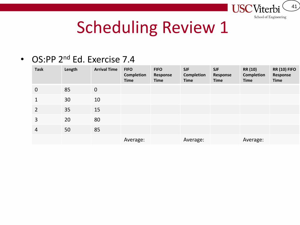
Scheduling Review 1

• OS:PP 2nd Ed. Exercise 7.4Task Length Arrival Time FIFO

Completion Time

FIFO Response Time

SJF Completion Time

SJF Response Time

RR (10)Completion Time

RR (10) FIFO Response Time

0 85 0

1 30 10

2 35 15

3 20 80

4 50 85

Average: Average: Average:

42

Scheduling Review 2

• OS:PP 2nd Ed. Exercise 7.13

– Task A: Arrives first at time 0, and uses the CPU for 100 ms before finishing

– Task B: Arrives shortly after A, still at time 0. Task B loops ten times; for each iteration of the loop B uses the CPU for 2ms and then it does I/O for 8ms.

– Task C: Identical to B but arrives after B, still at time 0

– Assume 0-time context switch, when will each task finish using:

Completion Time:

A B C

FIFO

RR (1 ms)

RR (100 ms)

SJF

MLFQ (highest priority = 1 ms time slice)

43

Scheduling Review 2 Answers

• OS:PP 2nd Ed. Exercise 7.13

– Task A: Arrives first at time 0, and uses the CPU for 100 ms before finishing

– Task B: Arrives shortly after A, still at time 0. Task B loops ten times; for each iteration of the loop B uses the CPU for 2ms and then it does I/O for 8ms.

– Task C: Identical to B but arrives after B, still at time 0

– Assume 0-time context switch, when will each task finish using:

Completion Time:

A B C

FIFO 100 200 300

RR (1 ms) 140 121 122

RR (100 ms) 100 200 22

SJF (on compute) 140 100 102

MLFQ (highest priority = 1 ms time slice)

142 104 106

44

QUEUEING THEORY

45

Motivation

• Queuing theory provides some mathematical model of a scheduling system that will allow us to perform "back of the envelope" calculations:

– Understand response time as a function of arrival rate or service (job execution) time

– Expected queue sizes

– Others

Server

Queuing

of Jobs

Arrivals

46

Definitions• λ (lambda) for arrival rate (e.g. 500 jobs/second)

• μ (mu) for service rate (e.g. 1000 jobs/second)

• S = 1/μ = service time

• W (Wait time) = Time spent waiting in a queue to be serviced

• R = Response time = Total time spent in the system– R = W + S

• U = Utilization = Percent of time the server is busy– λ/μ = when λ < μ

– 1 = when λ >= μ

– May not always want to maximize utilization

• X = Throughput (jobs processed per unit time)– Is X = μ or λ?

– X = λ when U < 1

– X = μ when U = 1

• N = Number of tasks in the system – Q + U = Number of waiters + Number of jobs being serviced

Server

Queuing

of Jobs

Arrivals

λ μN

47

Little's Law

• Stability: When λ < μ

– What if λ >= μ?

• Delay and queue length will grow without bound

• For a stable system (λ < μ)

– Little's Law says: N = X*R

• Number in the System (Waiters) = Throughput * Response Time

• Since over the long-term, throughput (X) = λ

– N = λ*(W+S) = λ*(W+(1/μ)) = λ*W + U

• If we expect 100 jobs/second & service time is 5 ms what utilization will our server run at?

– U = λ / μ = λ * S = 100 j/s * .005s = 0.5

• If 10,000 jobs arrive per second and experience 100 ms response time, what is the average number of jobs in the system:

– N = 10,000 * .1 = 1000

– True, regardless of what's inside the system

48

Inter-Arrival Times

• Much of the performance of a system depends on the distribution of interarrival times

• Assume λ < μ

– Example:

• λ = 1000 (1 job per 1 ms)

• μ = 2000 (1 job per 0.5 ms)

• Constant inter-arrival times: If jobs arrived exactly every 1 ms, what would Q (average occupancy/length of the queue) be?

– Q = 0 !! and R = 0.5 ms

– So do we not need a queue at all?

Response Time & Throughput as a

function of λ for

CONSTANT INTER-ARRIVAL times

49

Bursty Inter-Arrival Times

• Much of the performance of a system depends on the interarrival times

• Assume λ < μ

– Example:

• λ = 1000 (1 job per 1 ms)

• μ = 2000 (1 job per 0.5 ms)

• Bursty arrival times: But what if all 1000 jobs arrived at the t=0 sec. and then another 1000 jobs at t = 1 sec.

– Q ≈ 250

– R ≈ 250 ms

• Burstiness always increases response time

Response Time & Throughput as a

function of λ for

BURSTY INTER-ARRIVAL times

50

Modeling Arrivals

• So how should we model arrivals (i.e. inter-arrival time)

• Model both inter-arrival and service times using probabilistic distributions.

• Which distribution?

– Uniform

– Gaussian

– Exponential, p(t=x) = λe-λx because it is memoryless

• Memoryless: likelihood of an event occurring is independent of how long we've already waited or what other events have already happened

• This is just a model and not all workloads exhibit its characteristics but many do

51

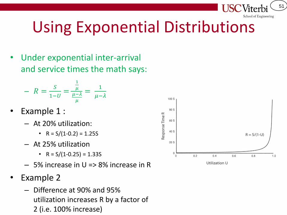
Using Exponential Distributions

• Under exponential inter-arrival and service times the math says:

– 𝑅 =𝑆

1−𝑈=

1

𝜇

𝜇−𝜆

𝜇

=1

𝜇−𝜆

• Example 1 :– At 20% utilization:

• R = S/(1-0.2) = 1.25S

– At 25% utilization• R = S/(1-0.25) = 1.33S

– 5% increase in U => 8% increase in R

• Example 2– Difference at 90% and 95%

utilization increases R by a factor of 2 (i.e. 100% increase)

52

What Ifs?

• Currently we are using FIFO scheduling; would other policies work better?– For exponential service times, FIFO works as well as RR because expected

service time remaining is independent of what's already there, you are better off finishing current jobs first

– So what about non-exponential distributions for service time?

– Many workloads for serving web pages and tasks in an OS are more burstyand exhibit so called heavy-tailed distributions

• More long tasks and more shorter tasks thus SJF and RR performs better than FIFO

– SJF is good, except it can greatly increase average response time at high utilization

• Why?

• Multiple servers: single queue or multiple queues– If multiple queues, the response time curve depends on arrivals to that queue

– If single queue, response time is always better (likelihood of being queued behind a large task is much less)

53

OVERLOAD MANAGEMENT

54

Overload Management

• What if burstiness causes a period where λ > μ– If you use RR what will happen?

• Sometime to give good service to some you must reject others

• What do we do when overload occurs?– Drop jobs

– Decrease service (throttle download bandwidth, disable certain features)

• Algorithms should be designed with overload in mind as many default applications will actually do MORE work under heavy loads– Caches under heavy load (thrashing)

– Naïve network protocols for resending packets when they don't reach the sender (they might have been dropped for a reason!)