Embed Size (px)
Citation preview

. . . . . .
.
......
CS711008Z Algorithm Design and AnalysisLecture 6. Basic algorithm design technique: Dynamic
programming
Dongbo Bu
Institute of Computing Technology
Chinese Academy of Sciences, Beijing, China
1 / 152

. . . . . .
.. Outline
The first example: MatrixChainMultiplication
Elements of dynamic programming technique;
Various ways to describe subproblems: Segmented LeastSquares, Knapsack, RNA Secondary Structure,Sequence Alignment, and Shortest Path;
Connection with greedy technique: Interval Scheduling,Shortest Path.
2 / 152

. . . . . .
..
Dynamic programming and its connection withdivide-and-conquer
Dynamic programming typically applies to the optimizationproblems if:
...1 The original problem can be divided into smaller subproblems,and
...2 The recursion among sub-problems has optimal-substructureproperty, i.e., the optimal solution to the original problem canbe calculated through combining the optimal solutions tosubproblems.
To identify meaningful recursions, one of the key steps is todefine an appropriate general form of sub-problems. Forthis aim, it is helpful to describe the solving process as amultiple-stage decision process.
Unlike the general divide-and-conqueror framework, a dynamicprogramming algorithm usually enumerate all possibledividing strategies. In addition, the repetition of computingthe common subproblems is avoided through “programing”.
3 / 152

. . . . . .
.. On what problems can we apply divide and conqueror?
Suppose a problem is related to the following data structure,perhaps we can try to divide it into sub-problems.
An array with n elementsA matrixA set of n elementsA treeA graph
4 / 152

. . . . . .
.
......
MatrixChainMultiplication problem: recursion oversequences
5 / 152

. . . . . .
.. MatrixChainMultiplication problem
.
......
INPUT:A sequence of n matrices A1, A2, ..., An; matrix Ai has dimensionpi−1 × pi;OUTPUT:Fully parenthesizing the product A1A2...An in a way to minimizethe number of scalar multiplications.
6 / 152

. . . . . .
.. Let’s start from a simple example
A1 =[1 2
]A2 =
[1 2 31 2 3
]A3 =
1 2 3 41 2 3 41 2 3 4
Solutions: ((A1)(A2))(A3) (A1)((A2)(A3))
#Multiplications: 1× 2× 3 2× 3× 4
+1× 3× 4 +1× 2× 4
= 18 = 32
Here we assume that the calculation of A1A2 needs 1× 2× 3scalar multiplications.
The objective is to determine a calculation sequence such thatthe number of multiplications is minimized.
7 / 152

. . . . . .
.. The solution space size
Intuitively, a calculation sequence can be described as a binarytree, where each node corresponds to a subproblem.
...............((A1)(A2))((A3)(A4))
.
((A1)(A2))
.
((A3)(A4))
.
(A1)
.
(A2)
.
(A3)
.
(A4)
The total number of possible calculation sequences:(2nn
)−
(2nn−1
)(Catalan number)
Thus, it takes exponential time to enumerate all possiblecalculation sequences.
Question: can we design an efficient algorithm?
8 / 152

. . . . . .
.
......A dynamic programming algorithm (by S. S. Godbole, 1973?)
9 / 152

. . . . . .
.. Defining general form of sub-problems
...1 It is not easy to solve the problem directly when n is large.Let’s investigate whether it is possible to reduce into smallersub-problems.
...2 Solution: a full parentheses. Let’s describe the solving processas a process of multiple-stage decisions, where eachdecision is to add parentheses at a position.
...3 Suppose we have already worked out the optimal solution O,where the first decision adds two parentheses as(A1...Ak)(Ak+1...An).
...4 This decision decomposes the original problem into twoindependent sub-problems: to calculate A1...Ak andAk+1...An.
...5 Summarizing these two cases, we define the general form ofsub-problems as: to calculate Ai...Aj with the minimalnumber of scalar multiplications.
10 / 152

. . . . . .
.. Optimal substructure property
The general form of sub-problems: to calculate Ai...Aj withthe minimal number of scalar multiplications. Let’s denote theoptimal solution value to the sub-problem as OPT (i, j), thusthe original problem can be solved via calculating OPT (1, n).
The optimal solution to the original problem can be obtainedthrough combining the optimal solutions to sub-problems.This recursion can be stated as the following optimalsubstructure property:OPT (1, n) = OPT (1, k) +OPT (k + 1, n) + p1pk+1pn+1
11 / 152

. . . . . .
.. Proof of the optimal substructure property
“Cut-and-paste” proof:
Suppose for A1...Ak, there is another parentheses OPT ′(1, k)better than OPT (1, k). Then the combination of OPT ′(1, k)and OPT (k + 1, n) leads to a new solution with lower costthan OPT (1, n): a contradiction.Here, the independence between A1...Ak and Ak+1...An
guarantees that the substitution of OPT (1, k) withOPT ′(1, k) does not affect solution to Ak+1...An.
12 / 152

. . . . . .
.. A recursive solution
So far so good! The only difficulty is that we have no idea ofthe first splitting position k in the optimal solution.
How to overcome this difficulty? Enumeration! Weenumerate all possible options of the first decision, i.e.for all k, i ≤ k < j.
.......
k = 1
.(A1)(A2A3A4)
.
(A1)
.
(A2A3A4)
......
k = 2
.(A1A2)(A3A4)
.
(A1A2)
.
(A3A4)
......
k = 3
.(A1A2A3)(A4)
.
(A1A2A3)
.
(A4)
Thus we have the following recursion:
OPT (i, j) =
{0 i = j
mini≤k<j{OPT (i, k) +OPT (k + 1, j) + pipk+1pj+1} otherwise
13 / 152

. . . . . .
.
......Implementing the recursion: trial 1
14 / 152

. . . . . .
.. Trial 1: Explore the recursion in the top-down manner
RECURSIVE MATRIX CHAIN(i, j)
1: if i == j then2: return 0;3: end if4: OPT (i, j) = +∞;5: for k = i to j − 1 do6: q = RECURSIVE MATRIX CHAIN(i, k)7: + RECURSIVE MATRIX CHAIN(k + 1, j)8: +pipk+1pj+1;9: if q < OPT (i, j) then
10: OPT (i, j) = q;11: end if12: end for13: return OPT (i, j);
Note: The optimal solution to the original problem can beobtained through callingRECURSIVE MATRIX CHAIN(1, n).
15 / 152

. . . . . .
.. An example
A1 =[1 2
]A2 =
[1 2 31 2 3
]A3 =
1 2 3 41 2 3 41 2 3 4
A4 =
1 2 3 4 51 2 3 4 51 2 3 4 51 2 3 4 5
1 × 2 2 × 3 3 × 4 4 × 5
....
A1
.
A4
..............A1A2A3A4
.
A1A2
.
A3A4
.
A1
.
A2
.
A3
.
A4
...
A1
.
A3
..............
A1A2A3
.
A2A3
.
A1A2
.
A2
.
A3
.
A1
.
A2
...
A4
.
A2
..............
A2A3A4
.
A3A4
.
A2A3
.
A3
.
A4
.
A2
.
A3
Note: each node of the recursion tree represents a subproblem.
16 / 152

. . . . . .
.. However, this is not a good implementation
.Theorem..
......
Algorithm RECURSIVE-MATRIX-CHAIN costs exponentialtime.
Let T (n) denote the time used to calculate product of nmatrices. Then T (n) ≥ 1 +
∑n−1k=1(T (k) + T (n− k) + 1) for
n > 1.
..
T (4)
...
A1
.
A4
.
T (1)
.
T (1)
..............A1A2A3A4
.
A1A2
.
A3A4
.
A1
.
A2
.
A3
.
A4
.
T (2)
.
T (2)
...
A1
.
A3
..............
A1A2A3
.
A2A3
.
A1A2
.
A2
.
A3
.
A1
.
A2
.
T (3)
...
A4
.
A2
..............
A2A3A4
.
A3A4
.
A2A3
.
A3
.
A4
.
A2
.
A3
.
T (3)
17 / 152

. . . . . .
.Proof...
......
We shall prove T (n) ≥ 2n−1 using the substitution technique.
Basis: T (1) ≥ 1 = 21−1.Induction:
T (n) ≥ 1 +∑n−1
k=1(T (k) + T (n− k) + 1) (1)
= n+ 2∑n−1
k=1T (k) (2)
≥ n+ 2∑n−1
k=12k−1 (3)
≥ n+ 2(2n−1 − 1) (4)
≥ n+ 2n − 2 (5)
≥ 2n−1 (6)
18 / 152

. . . . . .
.. Why the first trial failed?
....
A1
.
A4
..............A1A2A3A4
.
A1A2
.
A3A4
.
A1
.
A2
.
A3
.
A4
.......
A1
.
A3
..............
A1A2A3
.
A2A3
.
A1A2
.
A2
.
A3
.
A1
.
A2
.........
A4
.
A2
..............
A2A3A4
.
A3A4
.
A2A3
.
A3
.
A4
.
A2
.
A3
..
Reason: There are only O(n2) subproblems. However, somesubproblems (in red) were solved repeatedly.
Solution: memorize the solutions to subproblems using anarray OPT [1..n; 1..n] for further look-up.
19 / 152

. . . . . .
.
......Implementing the recursion: trial 2
20 / 152

. . . . . .
.. The “memorizing” technique
MEMORIZE MATRIX CHAIN(i, j)
1: if OPT [i, j] ̸= NULL then2: return OPT (i, j);3: end if4: if i == j then5: OPT [i, j] = 0;6: else7: for k = i to j − 1 do8: q = MEMORIZE MATRIX CHAIN(i, k)9: +MEMORIZE MATRIX CHAIN(k + 1, j)
10: +pipk+1pj+1;11: if q < OPT [i, j] then12: OPT [i, j] = q;13: end if14: end for15: end if16: return OPT [i, j];
21 / 152

. . . . . .
.. The “memorizing” technique cont’d
The original problem can be solved by callingMEMORIZE MATRIX CHAIN(1, n) with all OPT [i, j]initialized as NULL.
Time-complexity: O(n3) (The calculation of each entryOPT [i, j] makes O(n) recursive calls in line 8.)
Note: the calculation of Fibonacci number is a good exampleof the power of the “memorizing” technique.
22 / 152

. . . . . .
.
......Implementing the recursion faster: trial 3
23 / 152

. . . . . .
..
Trial 3: Faster implementation: unrolling the recursion inthe bottom-up manner
MATRIX CHAIN MULTIPLICATION(P )
1: for i = 1 to n do2: OPT (i, i) = 0;3: end for4: for l = 2 to n do5: for i = 1 to n− l + 1 do6: j = i+ l − 1;7: OPT (i, j) = +∞;8: for k = i to j − 1 do9: q = OPT (i, k) +OPT (k + 1, j) + pipk+1pj+1;
10: if q < OPT (i, j) then11: OPT (i, j) = q;12: S(i, j) = k;13: end if14: end for15: end for16: end for17: return OPT (1, n);
24 / 152
. . . . . .
..
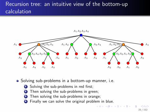
Recursion tree: an intuitive view of the bottom-upcalculation
....
A1
.
A4
..............A1A2A3A4
.
A1A2
.
A3A4
.
A1
.
A2
.
A3
.
A4
..........
A1
.
A3
..............
A1A2A3
.
A2A3
.
A1A2
.
A2
.
A3
.
A1
.
A2
..........
A4
.
A2
..............
A2A3A4
.
A3A4
.
A2A3
.
A3
.
A4
.
A2
.
A3
.......
Solving sub-problems in a bottom-up manner, i.e....1 Solving the sub-problems in red first;...2 Then solving the sub-problems in green;...3 Then solving the sub-problems in orange;...4 Finally we can solve the original problem in blue.
25 / 152
. . . . . .
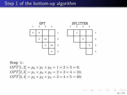
.. Step 1 of the bottom-up algorithm
..
OPT
.
1
.
2
.
3
.
4
.1
.2
.
3
.
4
.0
.6
...0
.24
..
0
.
60
.
0
.
SPLITTER
.
1
.
2
.
3
.
4
.1
.2
.
3
.
4
..1
....2
...
3
.
Step 1:
OPT [1, 2] = p0 × p1 × p2 = 1× 2× 3 = 6;OPT [2, 3] = p1 × p2 × p3 = 2× 3× 4 = 24;OPT [3, 4] = p2 × p3 × p4 = 3× 4× 5 = 60;
26 / 152

. . . . . .
.. Step 2 of the bottom-up algorithm
..
OPT
.
1
.
2
.
3
.
4
.1
.2
.
3
.
4
.0
.6
.18
..0
.24
.64
.
0
.
60
.
0
.
SPLITTER
.
1
.
2
.
3
.
4
.1
.2
.
3
.
4
..1
.2
...2
.3
..
3
.
Step 2:
OPT [1, 3] = min
{OPT [1, 2] +OPT [3, 3] + p0 × p2 × p3(= 18)
OPT [1, 1] +OPT [2, 3] + p0 × p1 × p3(= 32)
Thus, SPLITTER[1, 2] = 2.
OPT [2, 4] = min
{OPT [2, 2] +OPT [3, 4] + p1 × p2 × p4(= 90)
OPT [2, 3] +OPT [4, 4] + p1 × p3 × p4(= 64)
Thus, SPLITTER[2, 4] = 3.
27 / 152

. . . . . .
.. Step 3 of the bottom-up algorithm
..
OPT
.
1
.
2
.
3
.
4
.1
.2
.
3
.
4
.0
.6
.18
.38
.0
.24
.64
.
0
.
60
.
0
.
SPLITTER
.
1
.
2
.
3
.
4
.1
.2
.
3
.
4
..1
.2
.3
..2
.3
..
3
.
Step 3:
OPT [1, 4] = min
OPT [1, 1] +OPT [2, 4] + p0 × p1 × p4(= 74)
OPT [1, 2] +OPT [3, 4] + p0 × p2 × p4(= 81)
OPT [1, 3] +OPT [4, 4] + p0 × p3 × p4(= 38)
Thus, SPLITTER[1, 4] = 3.
28 / 152

. . . . . .
.
......
Question: We have calculated the optimal value, but how to getthe optimal calculation sequence?
29 / 152

. . . . . .
..
Final step: constructing an optimal solution through“backtracking” the optimal options
Idea: backtracking! Starting from OPT [1, n], we trace backthe source of OPT [1, n], i.e. which option we take at eachdecision stage.
Specifically, an auxiliary array S[1..n, 1..n] is used.
Each entry S[i, j] records the optimal decision, i.e. the valueof k such that the optimal parentheses of Ai...Aj occursbetween AkAk+1.Thus, the optimal solution to the original problem A1..n isA1..S[1,n]AS[1,n]+1..n.
Note: The optimal option cannot be determined beforesolving all subproblems.
30 / 152

. . . . . .
.. Backtracking: step 1
..
OPT
.
1
.
2
.
3
.
4
.1
.2
.
3
.
4
.0
.6
.18
.38
.0
.24
.64
.
0
.
60
.
0
.
SPLITTER
.
1
.
2
.
3
.
4
.1
.2
.
3
.
4
..1
.2
.3
..2
.3
..
3
.
Step 1: ( A1A2A3 ) ( A4 )
31 / 152
. . . . . .
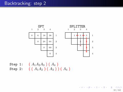
.. Backtracking: step 2
..
OPT
.
1
.
2
.
3
.
4
.1
.2
.
3
.
4
.0
.6
.18
.38
.0
.24
.64
.
0
.
60
.
0
.
SPLITTER
.
1
.
2
.
3
.
4
.1
.2
.
3
.
4
..1
.2
.3
..2
.3
..
3
.
Step 1: ( A1A2A3 ) ( A4 )Step 2: ( ( A1A2 ) ( A3 ) ) ( A4 )
32 / 152

. . . . . .
.. Backtracking: step 3
..
OPT
.
1
.
2
.
3
.
4
.1
.2
.
3
.
4
.0
.6
.18
.38
.0
.24
.64
.
0
.
60
.
0
.
SPLITTER
.
1
.
2
.
3
.
4
.1
.2
.
3
.
4
..1
.2
.3
..2
.3
..
3
.
Step 1: ( A1A2A3 ) ( A4 )Step 2: ( ( A1A2 ) ( A3 ) ) ( A4 )Step 3: ( ( ( A1 ) ( A2 ) ( A3 ) ) ( A4 )
33 / 152

. . . . . .
.. Summary: elements of dynamics programming
...1 It is usually not easy to solve a large problem directly. Let’s considerwhether the problem can be decomposed into smaller sub-problems.How to define sub-problems?
Let’s describe the solving process as a process of multiple-stagedecisions first.Suppose that we have already worked out the optimal solution. Let’sconsider the first/final decision (in some order) in the optimalsolution. The first/final decision might have several options.
We enumerate all possible options for the decision, and observe the
generated sub-problems. The general form of sub-problems can be
defined via summarising all possible forms of sub-problems.
...2 Show that the recursion among sub-problems can be stated as theoptimal substructure property, i.e. the optimal solution to the problemcontains within it optimal solutions to subproblems.
...3 Programming: if recursive algorithm solves the same subproblem over andover, “tabular” can be used to avoid the repetition of solving samesub-problems.
34 / 152

. . . . . .
.
......Question: is O(n3) the lower bound?
35 / 152

. . . . . .
.. An O(n log n) algorithm by Hu and Shing 1981
..
1
.
2
.
3
.
4
.
5
.
A1
.
A2
.
A3
.
A4
.
One-to-one correspondence between parenthesis andpartioning a convex polygon into non-intersecting triangles.
Each node has a weight wi, and a triangle corresponds to aproduct of the weight of its nodes.The decomposition (red, dashed lines) has a weight sum of 38.In fact, it corresponds to the parenthesis ( ( ( A1 ) ( A2 ) ( A3
) ) ( A4 ).
The optimal decomposition can be found in O(n log n) time.
(See Hu and Shing 1981 for details)36 / 152

. . . . . .
.
......0/1 Knapsack problem: recursion over sets
37 / 152

. . . . . .
.. A Knapsack instance
Consider a set of items, where each item has a weight and avalue. The objective is to select a subset of items such thatthe total weight is less than a given limit and the total valueis as large as possible.
38 / 152

. . . . . .
.. 0/1 Knapsack problem
.Formalized Definition:..
......
Input:A set of items S = {1, 2, ..., n}. Item i has weight wi andvalue vi. A total weight limit W ;
Output:A sub-set of items to maximize the total value with totalweight below W .
Here, “0/1” means that we should select an item (1) orabandon it (0), and we cannot select parts of an item.
In contrast, Fractional Knapsack problem allow one toselect a fractional, say 0.5, of an item.
39 / 152

. . . . . .
.. 0/1 Knapsack problem: an intuitive algorithm
Intuitive method: selecting “expensive” items first.
But this is not the optimal solution.
40 / 152
. . . . . .
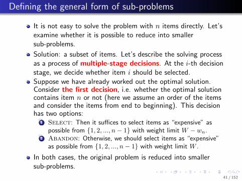
.. Defining the general form of sub-problems
It is not easy to solve the problem with n items directly. Let’sexamine whether it is possible to reduce into smallersub-problems.
Solution: a subset of items. Let’s describe the solving processas a process of multiple-stage decisions. At the i-th decisionstage, we decide whether item i should be selected.
Suppose we have already worked out the optimal solution.Consider the first decision, i.e. whether the optimal solutioncontains item n or not (here we assume an order of the itemsand consider the items from end to beginning). This decisionhas two options:
...1 Select: Then it suffices to select items as “expensive” aspossible from {1, 2, ..., n− 1} with weight limit W − wn.
...2 Abandon: Otherwise, we should select items as “expensive”as possible from {1, 2, ..., n− 1} with weight limit W .
In both cases, the original problem is reduced into smallersub-problems.
41 / 152

. . . . . .
.. Optimal sub-structure property
Summarizing these two cases, we can set the general form ofsub-problems as: to select items as “expensive” as possiblefrom {1, 2, ..., i} with weight limit w. Denote the optimalsolution value as OPT ({1, 2, ..., i}, w).Then we can prove the optimal sub-structure property:
OPT ({1, 2, ..., n},W ) = min
{OPT ({1, 2, ..., n− 1},W )
OPT ({1, 2, ..., n− 1},W − wn) + vn
42 / 152
. . . . . .
.. Algorithm
Knapsack(n,W )
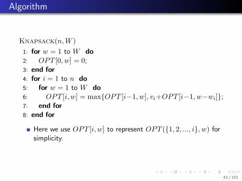
1: for w = 1 to W do2: OPT [0, w] = 0;3: end for4: for i = 1 to n do5: for w = 1 to W do6: OPT [i, w] = max{OPT [i−1, w], vi+OPT [i−1, w−wi]};7: end for8: end for
Here we use OPT [i, w] to represent OPT ({1, 2, ..., i}, w) forsimplicity.
43 / 152

. . . . . .
.. An example: Step 1
..
w1 = 2
.
v1 = 2
.
w2 = 2
.
v2 = 2
.
w3 = 3
.
v3 = 3
.
W = 6
Initially allOPT [0, w] = 0
w = 0 1 2 3 4 5 6
i = 3
i = 2
i = 1
i = 0 0 0 0 0 0 0 0
44 / 152

. . . . . .
.. Step 2
OPT [1, 2] = max{OPT [0, 2](= 0),OPT [0, 0] + V1(= 0 + 2)}
= 2
w = 0 1 2 3 4 5 6
i = 3
i = 2
i = 1 0 0 2 2 2 2 2
i = 0 0 0 0 0 0 0 0.
45 / 152

. . . . . .
.. Step 3
OPT [2, 4] = max{OPT [1, 4](= 2),OPT [1, 2] + V2(= 2 + 2)}
= 4
w = 0 1 2 3 4 5 6
i = 3
i = 2 0 0 2 2 4 4 4
i = 1 0 0 2 2 2 2 2
i = 0 0 0 0 0 0 0 0.
46 / 152

. . . . . .
.. Step 4
OPT [3, 3] = max{OPT [2, 3](= 2),OPT [2, 0] + V3(= 0 + 3)}
= 3
w = 0 1 2 3 4 5 6
i = 3 0 0 2 3 4 5 5
i = 2 0 0 2 2 4 4 4
i = 1 0 0 2 2 2 2 2
i = 0 0 0 0 0 0 0 0.
47 / 152

. . . . . .
.. Backtracking
OPT [3, 6] = max{OPT [2, 6](= 4),OPT [2, 3] + V3(= 2 + 3)}
= 5Decision: Select item 3
OPT [2, 3] = max{OPT [1, 3](= 2),OPT [1, 1] + V2(= 0 + 2)}
= 2Decision: Select item 2
w = 0 1 2 3 4 5 6
i = 3 0 0 2 3 4 5 5
i = 2 0 0 2 2 4 4 4
i = 1 0 0 2 2 2 2 2
i = 0 0 0 0 0 0 0 0.
48 / 152

. . . . . .
.. Time complexity analysis
Time complexity: O(nW ). (Hint: for each entry in thematrix, only a comparison is needed; we have O(nW ) entriesin the matrix.)
Notes:...1 This algorithm is inefficient when W is large, say W = 1M ....2 Remember that a polynomial time algorithm costs timepolynomial in the input length. However, this algorithm coststime mW = m2logW = m2input length. Exponential!
...3 Pseudo-polynomial time algorithm: polynominal in the valueof W rather than the length of W (logW ).
...4 We will revisit this algorithm in approximation algorithmdesign.
49 / 152

. . . . . .
.. Why should we consider items from end to beginning?
Let’s examine the following two types of selection of items:...1 If we consider an arbitrary item i, then the sub-problembecomes into “selecting items as expensive as possible from asubset s with weight limit w”. We have the followingrecursion:
OPT ({1, 2, ..., n},W ) = min
{OPT ({1, 2, ..., n} − {i},W )
OPT ({1, 2, ..., n} − {i},W − wi) + vi
...2 In contrast, if we assume an order of the items and considerthem from end to beginning, then the subproblem can be setas “selecting items as expensive as possible from {1, 2, ..., i}with weight limit w” and we have the following recursion:
OPT ({1, 2, ..., n},W ) = min
{OPT ({1, 2, ..., n− 1},W )
OPT ({1, 2, ..., n− 1},W − wn) + vn
In fact, the first one exploits recursion over sets, which leadsto an exponential number of subproblems. In contrast, thesecond one is a recursion over sequences and the number ofsubproblems is only O(nW ).
50 / 152

. . . . . .
.. Extension: The first public-key encryption system
Cryptosystems based on the knapsack problem were amongthe first public key systems to be invented, and for a whilewere considered to be among the most promising. However,essentially all of the knapsack cryptosystems that have beenproposed so far have been broken. These notes outline thebasic constructions of these cryptosystems and attacks thathave been developed on them.
See The Rise and Fall of Knapsack Cryptosystems for details.
51 / 152

. . . . . .
.
......Vertex Cover: recursion over trees
52 / 152

. . . . . .
.. Vertex Cover Problem
Practical problem:Given n sites connected with paths, how many guards (orcameras) should be deployed on sites to surveille all the paths?
.Formalized Definition:..
......
Input: Given a graph G =< V,E >Output: the minimum of nodes S ⊆ V , such that each edge hasat least one of its endpoints in S
For example, how many nodes are needed to cover all edges inthe following graph?
..................
53 / 152
. . . . . .
.. Defining general form of sub-problems
.........................
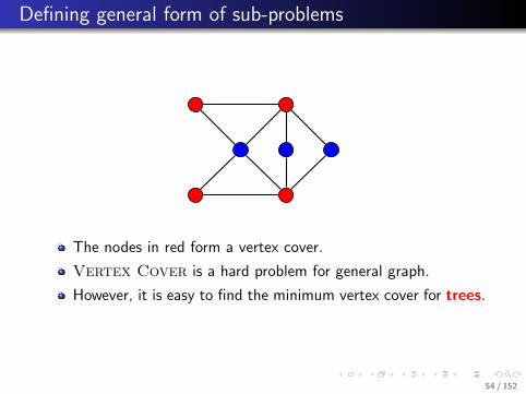
The nodes in red form a vertex cover.
Vertex Cover is a hard problem for general graph.
However, it is easy to find the minimum vertex cover for trees.
54 / 152
. . . . . .
.. Optimal sub-structure property
..0.
1
.
2
.
3
.
4
.
5
.
6
.
7
........root
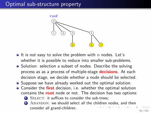
It is not easy to solve the problem with n nodes. Let’swhether it is possible to reduce into smaller sub-problems.Solution: selection a subset of nodes. Describe the solvingprocess as as a process of multiple-stage decisions. At eachdecision stage, we decide whether a node should be selected.Suppose we have already worked out the optimal solution.Consider the first decision, i.e. whether the optimal solutioncontains the root node or not. The decision has two options:
...1 Select: it suffices to consider the sub-trees;
...2 Abandon: we should select all the children nodes, and thenconsider all grand-children.
55 / 152
. . . . . .
.. An example
..0.
1
.
2
.
3
.
4
.
5
.
6
.
7
........root
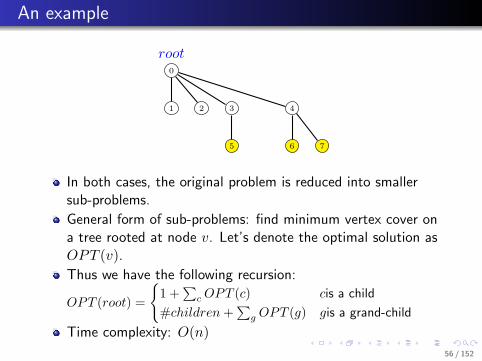
In both cases, the original problem is reduced into smallersub-problems.
General form of sub-problems: find minimum vertex cover ona tree rooted at node v. Let’s denote the optimal solution asOPT (v).
Thus we have the following recursion:
OPT (root) =
{1 +
∑c OPT (c) cis a child
#children+∑
g OPT (g) gis a grand-child
Time complexity: O(n)
56 / 152

. . . . . .
.
......
RNA Secondary Structure Prediction: recursion overtrees
57 / 152

. . . . . .
.. RNA secondary structure
RNA is a sequence of nucleic acids. It will automatically formstructures in water through the formation of bonds A−U andC −G.
The native structure is the conformation with the lowestenergy. Here, we simply use the number of base pairs as theenergy function.
58 / 152

. . . . . .
.. Formulation
.
......
INPUT:A sequence in alphabet Σ = {A,U,C,G};OUTPUT:A pairing scheme with the maximum pairing number
Requirements of base pairs:...1 Watson-Crick pair: A pairs with U , and C pairs with G;...2 There is no base occurring in more than 1 base pairs;...3 No cross-over (nesting): there is no crossover under theassumption of free pseudo-knots.
...4 And two bases i, j (|i− j| ≤ 4) cannot form a base pair.
59 / 152

. . . . . .
.. An example
60 / 152

. . . . . .
.. Nesting and Pseudo-knot
Left: nesting of base pairs (no cross-over); Right: pseudo-knots(cross-over).
61 / 152

. . . . . .
.. Feymann graph
Feymann graph: an intuitive representation form of RNAsecondary structure, i.e. two bases are connected by an edge ifthey form a Watson-Crick pair.
62 / 152

. . . . . .
.. Defining general form of sub-problems
Solution: a set of nested base pairs. Describe the solvingprocess as as a process of multiple-stage decisions. At thei-th decision stage, we determine whether base i forms pair ornot.
Suppose we have already worked out the optimal solution.
Consider the first decision made for base n. There are twooptions:
...1 Base n pairs with a base i: we should calculate optimal pairsfor regions i+ 1..n− 1 and 1..i− 1. Note that these twosub-problems are independent due to the “nested” property.
...2 Base n doesn’t form a pair: we should calculate optimal pairsfor regions 1..n− 1.
Thus we can design the general form of sub-problems as: tocalculate the optimal pairs for region i..j. (Denote theoptimal solution value as: OPT (i, j).)
63 / 152

. . . . . .
.. Optimal sub-structure property
Optimal substructures property:OPT (i, j) = max{OPT (i, j − 1),maxt{1 +OPT (i, t− 1) +OPT (t+ 1, j − 1)}}, where the second max takes over allpossible t such that t and j form a base pair. (Enumeratingall possible options for base n.)
64 / 152

. . . . . .
.. Algorithm
RNA2D(n)
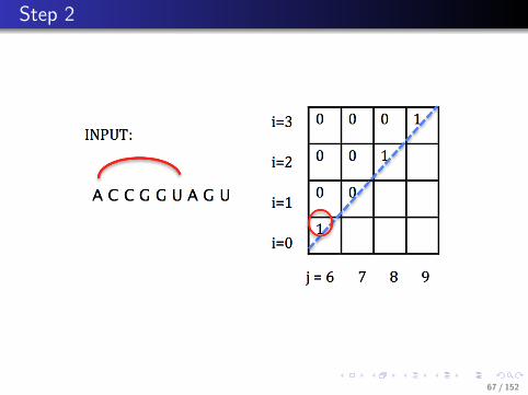
1: Initialize all OPT [i, j] with 0;2: for i = 1 to n do3: for j = i+ 5 to n do4: OPT [i, j] = max{OPT [i, j − 1],maxt{1 +OPT [i, t−
1] +OPT [t+ 1, j − 1]}};5: /* t and j can form Watson-Crick base pair. */6: end for7: end for
65 / 152

. . . . . .
.. An example: Step 1
66 / 152
. . . . . .
.. Step 2
67 / 152

. . . . . .
.. Step 3
68 / 152

. . . . . .
.. Step 4
Time complexity: O(n3).
69 / 152

. . . . . .
.. Extension: RNA is a good example of SCFG.
(see extra slides)
70 / 152

. . . . . .
.
......Sequence Alignment problem: recursion over sequence pairs
71 / 152

. . . . . .
.. Practical problem: genome similarity
To identify homology genes of two species, say Human andMouse. Human and Mouse NHPPEs (in KRAS genes) show a highsequence homology (Ref: Cogoi, S., et al. NAR, 2006).
..GGGCGGTGTG.
||| || | |
.
GGGAGG-GAG
Having calculating the similarity of genomes of various species, areasonable phylogeny tree can be estimated (Seehttps://www.llnl.gov/str/June05/Ovcharenko.html)
72 / 152

. . . . . .
.. Practical problem: spell tool to correct typos
When you type in ‘‘OCURRANCE’’, spell tools might guesswhat you really want to type through the following alignment,i.e. ‘‘OCURRANCE’’ is very similar to ‘‘OCCURRENCE’’
except for INS/DEL/MUTATION operations.
..O-CURRANCE.
| |||| |||
.
O-CURRANCE
73 / 152

. . . . . .
.. Sequence Alignment: formulation
.
......
INPUT:Two sequences S and T , |S| = m, and |T | = n;OUTPUT:To identify an alignment of S and T that maximizes a scoringfunction.
Note: for the sake of simplicity, the following indexing schema isused: S = S1S2...Sm.
74 / 152

. . . . . .
.. What is an alignment?
Alignment is usually used to describe the generating processof an erroneous word from the correct word using a series ofINS/DEL/MUTATION operations. . For example, thegenerating of “OCURRENCE” from “OCCURRANCE” can bedescribed as the following alignment:
..O-CURRENCE.
| |||| |||
.
O-CURRANCE
Here, ‘|’ represent identical characters.
For this aim, we make the two sequences to have the samelength through adding space ‘-’ at appropriate positions, whichchanges S into S′, and changes T to T ′ with identical length|S′| = |T ′|. There are three cases of aligned characters:
...1 T ′[i] = ‘−′: S′[i] is simply an INSERTION.
...2 S′[i] = ‘−′: S′[i] is simply a DELETION of T ′[i].
...3 Otherwise, S′[i] is a copy of T ′[i] (with possible MUTATION).
75 / 152

. . . . . .
..
How to measure an alignment in the sense of sequencesimilarity?
The similarity is defined as the linear sum of score of alignedletter pairs, i.e.
s(S, T ) =
|S′|∑i=1
s(S′[i], T ′[i])
Here we assume a simple setting of s(a, b) as follows:...1 Match: +1 , e.g. s(‘C ′, ‘C ′) = 1....2 Mismatch: -1, e.g. s(‘E′, ‘A′) = −1....3 Insertion/Deletion: -3, e.g. s(‘C ′, ‘−′) = −3.
1
1Ideally, the score function is designed such that s(S, T ) is proportional tolog Pr[Sis generated from T ]. See extra slides for the statistical model forsequence alignment, and better similarity definition, say BLOSUM62, PAM250substitution matrix, etc.
76 / 152

. . . . . .
.. Alignment is useful
Observation 1: Using alignment, we can determine the mostlikely source of “OCURRANCE”.
...1 T = “OCCURRENCE”:..S’: O-CURRANCE.
| |||| |||
.
T’: OCCURRENCE
s(S′, T ′) = 1− 3 + 1 + 1 + 1 + 1− 1 + 1 + 1 + 1 = 4...2 T =“OCCUPATION”:
..S’: OC-URRA---NCE.
|| | | |
.
T’: OCCU-PATION--
s(S′, T ′) = 1+1−3+1−3−3−1+1−3−3−3+1−3−3 = −28
Conjecture: it is more likely that “OCURRANCE” comes from“OCCURRENCE” relative to “OCCUPATION”.
77 / 152

. . . . . .
.. Alignment is useful cont’d
Observation 2: In addition, we can also determine the mostlikely operations changing “OCCURRENCE” into “OCURRANCE”.
...1 Alignment 1:
..S’: O-CURRANCE.
| |||| |||
.
T’: OCCURRENCE
s(S′, T ′) = 1− 3 + 1 + 1 + 1 + 1− 1 + 1 + 1 + 1 = 4...2 Alignment 2:
..S’: O-CURR-ANCE.
| |||| |||
.
T’: OCCURRE-NCE
s(S′, T ′) = 1− 3 + 1 + 1 + 1− 3− 3 + 1 + 1 + 1 = −1
Conjecture: the first alignment might describes the realgenerating process of “OCURRANCE” from “OCCURRENCE”.
78 / 152

. . . . . .
.. The general form of sub-problems and recursions I
It is not easy to consider long sequences directly. Let’sconsider whether it is possible to reduce into smallersubproblem.
Solution: finding some positions to insert ‘-’ to represent thegenerating process of S from T . Let’s describe the solvingprocess as as a process of multiple-stage decisions. At eachdecision stage, we decide whether Si aligns with Tj (match),Si aligns with a ‘-’ (insert), or Tj aligns with a ‘-’ (deletion).
..
Match
.S: .O. C. U. R. R. A. N. C. E.
T:
.
O
.
C
.
C
.
U
.
R
.
R
.
E
.
N
.
C
.
E
.
Insertion
. S:. O. C. U. R. R. A. N. C. E.
T:
.
O
.
C
.
C
.
U
.
R
.
R
.
E
.
N
.
C
.
E
.
-
.
Deletion
. S:. O. C. U. R. R. A. N. C. E. -.
T:
.
O
.
C
.
C
.
U
.
R
.
R
.
E
.
N
.
C
.
E
79 / 152

. . . . . .
.. The general form of sub-problems and recursions II
Suppose we have already worked out the optimal solution.Consider the first decision made for Sm. There are threecases:
...1 Sm pairs with Tn, i.e. Sm comes from Tn. Then it suffices toalign S[1..m− 1] and T [1..n− 1];
...2 Sm pairs with a space ‘-’, i.e. Sm is an INSERTION. Then weneed to align S[1..m− 1] and T [1..n];
...3 Tn pairs with a space ‘-’, i.e. Sm is a DELETION of a letter inT . Then we need to align S[1..m] and T [1..n− 1].
In the three cases, the original problem can be reduced intosmaller sub-problems.
..
Match
.S: .O. C. U. R. R. A. N. C. E.
T:
.
O
.
C
.
C
.
U
.
R
.
R
.
E
.
N
.
C
.
E
.
Insertion
. S:. O. C. U. R. R. A. N. C. E.
T:
.
O
.
C
.
C
.
U
.
R
.
R
.
E
.
N
.
C
.
E
.
-
.
Deletion
. S:. O. C. U. R. R. A. N. C. E. -.
T:
.
O
.
C
.
C
.
U
.
R
.
R
.
E
.
N
.
C
.
E
80 / 152

. . . . . .
.. The general form of sub-problems and recursions III
Thus, we can design the general form of sub-problems as:alignment a prefix of S (denoted as S[1..i]) and prefix of T(denoted as T [1..j]). Denote the optimal solution value asOPT (i, j).
We can prove the following optimal substructure property:
OPT (i, j) = max
s(Si, Tj) +OPT (i− 1, j − 1)s(‘ ′, Tj) +OPT (i, j − 1)s(Si, ‘
′) +OPT (i− 1, j)
81 / 152

. . . . . .
.. Needleman-Wunsch algorithm [1970]
Needleman-Wunsch(S, T )
1: for i = 0 to m; do2: OPT [i, 0] = −3 ∗ i;3: end for4: for j = 0 to n; do5: OPT [0, j] = −3 ∗ j;6: end for7: for i = 1 to m do8: for j = 1 to n do9: OPT [i, j] = max{OPT [i− 1, j − 1] + s(Si, Tj), OPT [i−
1, j]− 3, OPT [i, j − 1]− 3};10: end for11: end for12: return OPT [m,n] ;
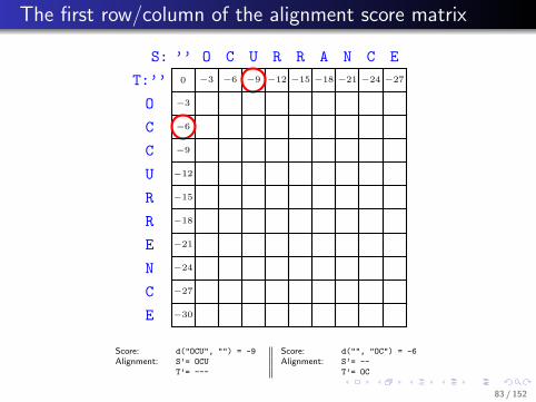
Note: the first row is introduced to describe the alignment ofprefixes T [1..i] with an empty sequence ϵ, so does the first column.
82 / 152
. . . . . .
.. The first row/column of the alignment score matrix
..
S:
.
’’
.
O
.
C
.
U
.
R
.
R
.
A
.
N
.
C
.
E
.T:’’ .O
.
C
.
C
.
U
.
R
.
R
.
E
.
N
.
C
.
E
.0
.−3
.−6
.−9
.−12
.−15
.−18
.−21
.−24
.−27
.−3
..........
−6
..........
−9
..........
−12
..........
−15
..........
−18
..........
−21
..........
−24
..........
−27
..........
−30
.........
Score: d("OCU", "") = -9 Score: d("", "OC") = -6
Alignment: S’= OCU Alignment: S’= --
T’= --- T’= OC
83 / 152

. . . . . .
.. Why should we introduce the first row/column?
..
S:
.
’’
.
O
.
C
.
U
.
R
.
R
.
A
.
N
.
C
.
E
.T:’’ .O
.
C
.
C
.
U
.
R
.
R
.
E
.
N
.
C
.
E
.0
.−3
.−6
.−9
.−12
.−15
.−18
.−21
.−24
.−27
.−3
.1
.−2
.−5
.−8
.−11
.−14
.−17
.−20
.−23
.
−6
.
−2
.
2
.
−1
.
−4
.
−7
.
−10
.
−13
.
−16
.
−19
.
−9
.
−5
.
−1
.
1
.
−2
.
−5
.
−8
.
−11
.
−12
.
−15
.
−12
.
−8
.
−4
.
0
.
0
.
−3
.
−6
.
−9
.
−12
.
13
.
−15
.
−11
.
−7
.
−3
.
1
.
1
.
−2
.
−5
.
−8
.
−11
.
−18
.
−14
.
−10
.
−6
.
−2
.
2
.
0
.
−3
.
−6
.
−9
.
−21
.
−17
.
−13
.
−9
.
−5
.
−1
.
1
.
−1
.
−4
.
−5
.
−24
.
−20
.
−16
.
−12
.
−8
.
−4
.
−2
.
2
.
−1
.
−4
.
−27
.
−23
.
−19
.
−15
.
−11
.
−7
.
−5
.
−1
.
3
.
0
.
−30
.
−26
.
−22
.
−18
.
−14
.
−10
.
−8
.
−4
.
0
.
4
Score: d("OC", "O") = max
d(“OC“,““) −3 (=-9)d(“O“,““) −1 (=-4)d(“O“,“O“) −3 (=-2)
Alignment: S’= OC
T’= O- 84 / 152

. . . . . .
.. General cases
..
S:
.
’’
.
O
.
C
.
U
.
R
.
R
.
A
.
N
.
C
.
E
.T:’’ .O
.
C
.
C
.
U
.
R
.
R
.
E
.
N
.
C
.
E
.0
.−3
.−6
.−9
.−12
.−15
.−18
.−21
.−24
.−27
.−3
.1
.−2
.−5
.−8
.−11
.−14
.−17
.−20
.−23
.
−6
.
−2
.
2
.
−1
.
−4
.
−7
.
−10
.
−13
.
−16
.
−19
.
−9
.
−5
.
−1
.
1
.
−2
.
−5
.
−8
.
−11
.
−12
.
−15
.
−12
.
−8
.
−4
.
0
.
0
.
−3
.
−6
.
−9
.
−12
.
13
.
−15
.
−11
.
−7
.
−3
.
1
.
1
.
−2
.
−5
.
−8
.
−11
.
−18
.
−14
.
−10
.
−6
.
−2
.
2
.
0
.
−3
.
−6
.
−9
.
−21
.
−17
.
−13
.
−9
.
−5
.
−1
.
1
.
−1
.
−4
.
−5
.
−24
.
−20
.
−16
.
−12
.
−8
.
−4
.
−2
.
2
.
−1
.
−4
.
−27
.
−23
.
−19
.
−15
.
−11
.
−7
.
−5
.
−1
.
3
.
0
.
−30
.
−26
.
−22
.
−18
.
−14
.
−10
.
−8
.
−4
.
0
.
4
Score: d("OCUR", "OC") = max
d(“OCUR“,“O“) −3 (=-11)d(“OCU“,“O“) −1 (=-6)d(“OCU“,“OC“) −3 (=-4)
Alignment: S’= OCUR
T’= OC-- 85 / 152

. . . . . .
.. The final entry
..
S:
.
’’
.
O
.
C
.
U
.
R
.
R
.
A
.
N
.
C
.
E
.T:’’ .O
.
C
.
C
.
U
.
R
.
R
.
E
.
N
.
C
.
E
.0
.−3
.−6
.−9
.−12
.−15
.−18
.−21
.−24
.−27
.−3
.1
.−2
.−5
.−8
.−11
.−14
.−17
.−20
.−23
.
−6
.
−2
.
2
.
−1
.
−4
.
−7
.
−10
.
−13
.
−16
.
−19
.
−9
.
−5
.
−1
.
1
.
−2
.
−5
.
−8
.
−11
.
−12
.
−15
.
−12
.
−8
.
−4
.
0
.
0
.
−3
.
−6
.
−9
.
−12
.
13
.
−15
.
−11
.
−7
.
−3
.
1
.
1
.
−2
.
−5
.
−8
.
−11
.
−18
.
−14
.
−10
.
−6
.
−2
.
2
.
0
.
−3
.
−6
.
−9
.
−21
.
−17
.
−13
.
−9
.
−5
.
−1
.
1
.
−1
.
−4
.
−5
.
−24
.
−20
.
−16
.
−12
.
−8
.
−4
.
−2
.
2
.
−1
.
−4
.
−27
.
−23
.
−19
.
−15
.
−11
.
−7
.
−5
.
−1
.
3
.
0
.
−30
.
−26
.
−22
.
−18
.
−14
.
−10
.
−8
.
−4
.
0
.
4
Score: d("OCURRANCE", "OCCURRENCE") = max
d(“OCURRANCE“,“OCCURRENC“) −3 (=-3)d(“OCURRANC“,“OCCURRENC“) +1 (=4)d(“OCURRANC“,“OCCURRENCE“) −3 (=-3)
Alignment: S’= O-CURRANCE
T’= OCCURRENCE 86 / 152

. . . . . .
.
......Question: how to find the alignment with the highest score?
87 / 152

. . . . . .
.. Find the optimal alignment via backtracking
..
S:
.
’’
.
O
.
C
.
U
.
R
.
R
.
A
.
N
.
C
.
E
.T:’’ .O
.
C
.
C
.
U
.
R
.
R
.
E
.
N
.
C
.
E
.0
.−3
.−6
.−9
.−12
.−15
.−18
.−21
.−24
.−27
.−3
.1
.−2
.−5
.−8
.−11
.−14
.−17
.−20
.−23
.
−6
.
−2
.
2
.
−1
.
−4
.
−7
.
−10
.
−13
.
−16
.
−19
.
−9
.
−5
.
−1
.
1
.
−2
.
−5
.
−8
.
−11
.
−12
.
−15
.
−12
.
−8
.
−4
.
0
.
0
.
−3
.
−6
.
−9
.
−12
.
13
.
−15
.
−11
.
−7
.
−3
.
1
.
1
.
−2
.
−5
.
−8
.
−11
.
−18
.
−14
.
−10
.
−6
.
−2
.
2
.
0
.
−3
.
−6
.
−9
.
−21
.
−17
.
−13
.
−9
.
−5
.
−1
.
1
.
−1
.
−4
.
−5
.
−24
.
−20
.
−16
.
−12
.
−8
.
−4
.
−2
.
2
.
−1
.
−4
.
−27
.
−23
.
−19
.
−15
.
−11
.
−7
.
−5
.
−1
.
3
.
0
.
−30
.
−26
.
−22
.
−18
.
−14
.
−10
.
−8
.
−4
.
0
.
4
Optimal Alignment: S’= O-CURRANCE
T’= OCCURRENCE
88 / 152

. . . . . .
.. Optimal alignment versus sub-optimal alignments
In practice, there are always multiple alignments with nearlythe same score as the optimal alignment. Such alignments arecalled sub-optimal alignments and can be divided into thefollowing two categories.
Similar sub-optimal alignments: Some sub-optimal alignmentsdiffer from the optimal alignment in a few positions. Becausevariations might occur independently at different positions, thenumber of sub-optimal alignments grow exponentially with thedifference to the optimal alignment. The typical sub-optimalalignments can be obtained through sampling over thedynamic programming matrix.Distinct sub-optimal alignments: The other sub-optimalalignments differ completely from the optimal alignment.These sub-optimal alignments frequently appear when one orboth sequences have repeats.
Please refer to Biological Sequence Analysis: Probabilistic Modelsof Proteins and Nucleic Acids for details.
89 / 152

. . . . . .
.
......
Space efficient algorithm: reducing the space requirement fromO(mn) to O(m+ n) (D. S. Hirschberg, 1975)
90 / 152

. . . . . .
.. Technique 1: two arrays are enough if only score is needed
Key observation 1: it is easy to calculate the final scoreOPT (S, T ) only, i.e. the alignment information are notrecorded.
..
S:
.
’’
.
O
.
C
.
U
.
R
.
R
.
A
.
N
.
C
.
E
.T:’’ .O
.
C
.
C
.
U
.
R
.
R
.
E
.
N
.
C
.
E
.0
.−3
.−6
.−9
.−12
.−15
.−18
.−21
.−24
.−27
.−3
.1
.−2
.−5
.−8
.−11
.−14
.−17
.−20
.−23
.
−6
.
−2
.
2
.
−1
.
−4
.
−7
.
−10
.
−13
.
−16
.
−19
.
−9
.
−5
.
−1
.
1
.
−2
.
−5
.
−8
.
−11
.
−12
.
−15
.
−12
.
−8
.
−4
.
0
.
0
.
−3
.
−6
.
−9
.
−12
.
13
.
−15
.
−11
.
−7
.
−3
.
1
.
1
.
−2
.
−5
.
−8
.
−11
.
−18
.
−14
.
−10
.
−6
.
−2
.
2
.
0
.
−3
.
−6
.
−9
.
−21
.
−17
.
−13
.
−9
.
−5
.
−1
.
1
.
−1
.
−4
.
−5
.
−24
.
−20
.
−16
.
−12
.
−8
.
−4
.
−2
.
2
.
−1
.
−4
.
−27
.
−23
.
−19
.
−15
.
−11
.
−7
.
−5
.
−1
.
3
.
0
.
−30
.
−26
.
−22
.
−18
.
−14
.
−10
.
−8
.
−4
.
0
.
4
91 / 152

. . . . . .
.. Technique 1: two arrays are enough if only score is needed
Why? Only column j − 1 is needed to calculate column i. Thus, we
use two arrays score[1..n] and newscore[1..n] instead of the matrix
OPT [1..n, 1..m].
..
S:
.
’’
.
O
.
C
.
U
.
R
.
R
.
A
.
N
.
C
.
E
.T: ’’.O
.
C
.
C
.
U
.
R
.
R
.
E
.
N
.
C
.
E
.0
.−3
.−6
.−9
.−12
.−15
.−18
.−21
.−24
.−27
.−3
.1
.−2
.−5
.−8
.−11
.−14
.−17
.−20
.−23
.
−6
.
−2
.
2
.
−1
.
−4
.
−7
.
−10
.
−13
.
−16
.
−19
.
−9
.
−5
.
−1
.
1
.
−2
.
−5
.
−8
.
−11
.
−12
.
−15
.
−12
.
−8
.
−4
.
0
.
0
.
−3
.
−6
.
−9
.
−12
.
13
.
−15
.
−11
.
−7
.
−3
.
1
.
1
.
−2
.
−5
.
−8
.
−11
.
−18
.
−14
.
−10
.
−6
.
−2
.
2
.
0
.
−3
.
−6
.
−9
.
−21
.
−17
.
−13
.
−9
.
−5
.
−1
.
1
.
−1
.
−4
.
−5
.
−24
.
−20
.
−16
.
−12
.
−8
.
−4
.
−2
.
2
.
−1
.
−4
.
−27
.
−23
.
−19
.
−15
.
−11
.
−7
.
−5
.
−1
.
3
.
0
.
−30
.
−26
.
−22
.
−18
.
−14
.
−10
.
−8
.
−4
.
0
.
4
92 / 152

. . . . . .
.. Technique 1: two arrays are enough if only score is needed
Why? Only column j − 1 is needed to calculate column i. Thus, we
use two arrays score[1..n] and newscore[1..n] instead of the matrix
OPT [1..n, 1..m].
..
S:
.
’’
.
O
.
C
.
U
.
R
.
R
.
A
.
N
.
C
.
E
.T: ’’.O
.
C
.
C
.
U
.
R
.
R
.
E
.
N
.
C
.
E
.0
.−3
.−6
.−9
.−12
.−15
.−18
.−21
.−24
.−27
.−3
.1
.−2
.−5
.−8
.−11
.−14
.−17
.−20
.−23
.
−6
.
−2
.
2
.
−1
.
−4
.
−7
.
−10
.
−13
.
−16
.
−19
.
−9
.
−5
.
−1
.
1
.
−2
.
−5
.
−8
.
−11
.
−12
.
−15
.
−12
.
−8
.
−4
.
0
.
0
.
−3
.
−6
.
−9
.
−12
.
13
.
−15
.
−11
.
−7
.
−3
.
1
.
1
.
−2
.
−5
.
−8
.
−11
.
−18
.
−14
.
−10
.
−6
.
−2
.
2
.
0
.
−3
.
−6
.
−9
.
−21
.
−17
.
−13
.
−9
.
−5
.
−1
.
1
.
−1
.
−4
.
−5
.
−24
.
−20
.
−16
.
−12
.
−8
.
−4
.
−2
.
2
.
−1
.
−4
.
−27
.
−23
.
−19
.
−15
.
−11
.
−7
.
−5
.
−1
.
3
.
0
.
−30
.
−26
.
−22
.
−18
.
−14
.
−10
.
−8
.
−4
.
0
.
4
93 / 152

. . . . . .
.. Technique 1: two arrays are enough if only score is needed
Why? Only column j − 1 is needed to calculate column i. Thus, we
use two arrays score[1..m] and newscore[1..m] instead of the
matrix OPT [1..m, 1..n].
..
S:
.
’’
.
O
.
C
.
U
.
R
.
R
.
A
.
N
.
C
.
E
.T: ’’.O
.
C
.
C
.
U
.
R
.
R
.
E
.
N
.
C
.
E
.0
.−3
.−6
.−9
.−12
.−15
.−18
.−21
.−24
.−27
.−3
.1
.−2
.−5
.−8
.−11
.−14
.−17
.−20
.−23
.
−6
.
−2
.
2
.
−1
.
−4
.
−7
.
−10
.
−13
.
−16
.
−19
.
−9
.
−5
.
−1
.
1
.
−2
.
−5
.
−8
.
−11
.
−12
.
−15
.
−12
.
−8
.
−4
.
0
.
0
.
−3
.
−6
.
−9
.
−12
.
13
.
−15
.
−11
.
−7
.
−3
.
1
.
1
.
−2
.
−5
.
−8
.
−11
.
−18
.
−14
.
−10
.
−6
.
−2
.
2
.
0
.
−3
.
−6
.
−9
.
−21
.
−17
.
−13
.
−9
.
−5
.
−1
.
1
.
−1
.
−4
.
−5
.
−24
.
−20
.
−16
.
−12
.
−8
.
−4
.
−2
.
2
.
−1
.
−4
.
−27
.
−23
.
−19
.
−15
.
−11
.
−7
.
−5
.
−1
.
3
.
0
.
−30
.
−26
.
−22
.
−18
.
−14
.
−10
.
−8
.
−4
.
0
.
4
94 / 152

. . . . . .
.. Algorithm
Prefix Space Efficient Alignment(S, T, score)
1: for i = 0 to m do2: score[i] = −3 ∗ i;3: end for4: for i = 1 to m do5: newscore[0] = 0;6: for j = 1 to n do7: newscore[j] = max{score[j − 1] + s(Si, Tj), score[j]−
3, newscore[j − 1]− 3};8: end for9: for j = 1 to n do
10: score[j] = newscore[j];11: end for12: end for13: return score[n];
95 / 152
. . . . . .
.. Technique 2: aligning suffixes instead of prefixes
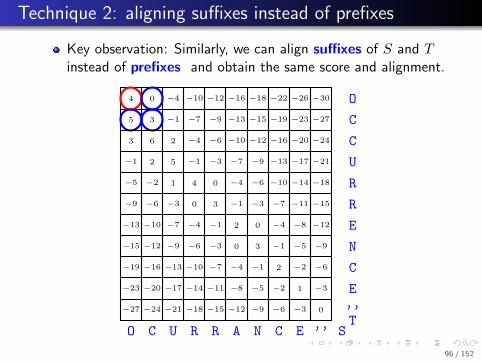
Key observation: Similarly, we can align suffixes of S and Tinstead of prefixes and obtain the same score and alignment.
..
S
.
’’
.
O
.
C
.
U
.
R
.
R
.
A
.
N
.
C
.
E
.
’’
. O.C
.
C
.
U
.
R
.
R
.
E
.
N
.
C
.
E
.
T
.4
.0
.−4
.−10
.−12
.−16
.−18
.−22
.−26
.−30
.5
.3
.−1
.−7
.−9
.−13
.−15
.−19
.−23
.−27
.
3
.
6
.
2
.
−4
.
−6
.
−10
.
−12
.
−16
.
−20
.
−24
.
−1
.
2
.
5
.
−1
.
−3
.
−7
.
−9
.
−13
.
−17
.
−21
.
−5
.
−2
.
1
.
4
.
0
.
−4
.
−6
.
−10
.
−14
.
−18
.
−9
.
−6
.
−3
.
0
.
3
.
−1
.
−3
.
−7
.
−11
.
−15
.
−13
.
−10
.
−7
.
−4
.
−1
.
2
.
0
.
−4
.
−8
.
−12
.
−15
.
−12
.
−9
.
−6
.
−3
.
0
.
3
.
−1
.
−5
.
−9
.
−19
.
−16
.
−13
.
−10
.
−7
.
−4
.
−1
.
2
.
−2
.
−6
.
−23
.
−20
.
−17
.
−14
.
−11
.
−8
.
−5
.
−2
.
1
.
−3
.
−27
.
−24
.
−21
.
−18
.
−15
.
−12
.
−9
.
−6
.
−3
.
0
96 / 152

. . . . . .
.. Final difficulty: identify optimal alignment besides score
...1 However, the optimal alignment cannot be restored viabacktracking since only the recent two columns of thematrix were kept.
...2 A clever idea: Suppose we have already obtained the optimalalignment. Let’s consider the position where S[m
2] is aligned
to (denoted as q). We have:
OPT (S, T ) = OPT (S[1..m
2], T [1..q])+OPT (S[
m
2+1..m], T [q+1..n])
...3 The equality holds due to the linearity of s(S, T ), and m2 is
chosen for the sake of time-complexity analysis.
..
m2
.S: .O. C. U. R.. R. A. N. C. E.
T:
.
O
.
C
.
C
.
U
.
R
..
R
.
E
.
N
.
C
.
E
.
1 ≤ q ≤ n
97 / 152
. . . . . .
.. Hirschberg’s algorithm for alignment
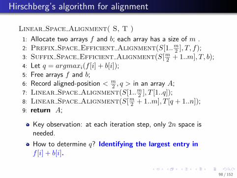
Linear Space Alignment( S, T )
1: Allocate two arrays f and b; each array has a size of m .2: Prefix Space Efficient Alignment(S[1..m2 ], T, f);3: Suffix Space Efficient Alignment(S[m2 + 1..m], T, b);4: Let q = argmaxi(f [i] + b[i]);5: Free arrays f and b;6: Record aligned-position < m
2 , q > in an array A;7: Linear Space Alignment(S[1..m2 ], T [1..q]);8: Linear Space Alignment(S[m2 + 1..m], T [q + 1..n]);9: return A;
Key observation: at each iteration step, only 2n space isneeded.
How to determine q? Identifying the largest entry inf [i] + b[i].
98 / 152

. . . . . .
.. Step 1: Determine the optimal aligned position of S[m2 ]
..
S:
.
’’
.
O
.
C
.
U
.
R
.T: ’’ .O
.
C
.
C
.
U
.
R
.
R
.
E
.
N
.
C
.
E
.0
.−3
.−6
.−9.
−12.
−3
.1
.−2
.−5
.−8
.
−6
.
−2
.
2
.
−1
.
−4
.
−9
.
−5
.
−1
.
1
.
−2
.
−12
.
−8
.
−4
.
0
.
0
.
−15
.
−11
.
−7
.
−3
.
1
.
−18
.
−14
.
−10
.
−6
.
−2
.
−21
.
−17
.
−13
.
−9
.
−5
.
−24
.
−20
.
−16
.
−12
.
−8
.
−27
.
−23
.
−19
.
−15
.
−11
.
−30
.
−26
.
−22
.
−18
.
−14
.
S
.
’’
.
R
.
A
.
N
.
C
.
E
.
’’
. O.C
.
C
.
U
.
R
.
R
.
E
.
N
.
C
.
E
.
T
.−12
.−16
.−18
.−22
.−26
.−30
.−9
.−13
.−15
.−19
.−23
.−27
.
−6
.
−10
.
−12
.
−16
.
−20
.
−24
.
−3
.
−7
.
−9
.
−13
.
−17
.
−21
.
0
.
−4
.
−6
.
−10
.
−14
.
−18
.
3
.
−1
.
−3
.
−7
.
−11
.
−15
.
−1
.
2
.
0
.
−4
.
−8
.
−12
.
−3
.
0
.
3
.
−1
.
−5
.
−9
.
−7
.
−4
.
−1
.
2
.
−2
.
−6
.
−11
.
−8
.
−5
.
−2
.
1
.
−3
.
−15
.
−12
.
−9
.
−6
.
−3
.
0
.−24
.−17
.
−10
.
−5
.
0
.
4
.
−3
.
−8
.
−15
.
−22
.
−25
.
4
.
f
.
f + b
.
b
The value of the largest item is 4, which is actually the optimal score
OPT (S, T ).99 / 152
. . . . . .
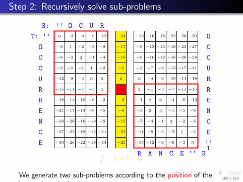
.. Step 2: Recursively solve sub-problems
..
S:
.
’’
.
O
.
C
.
U
.
R
.T: ’’ .O
.
C
.
C
.
U
.
R
.
R
.
E
.
N
.
C
.
E
.0
.−3
.−6
.−9.
−12.
−3
.1
.−2
.−5
.−8
.
−6
.
−2
.
2
.
−1
.
−4
.
−9
.
−5
.
−1
.
1
.
−2
.
−12
.
−8
.
−4
.
0
.
0
.
−15
.
−11
.
−7
.
−3
.
1
.
−18
.
−14
.
−10
.
−6
.
−2
.
−21
.
−17
.
−13
.
−9
.
−5
.
−24
.
−20
.
−16
.
−12
.
−8
.
−27
.
−23
.
−19
.
−15
.
−11
.
−30
.
−26
.
−22
.
−18
.
−14
.
S
.
’’
.
R
.
A
.
N
.
C
.
E
.
’’
. O.C
.
C
.
U
.
R
.
R
.
E
.
N
.
C
.
E
.
T
.−12
.−16
.−18
.−22
.−26
.−30
.−9
.−13
.−15
.−19
.−23
.−27
.
−6
.
−10
.
−12
.
−16
.
−20
.
−24
.
−3
.
−7
.
−9
.
−13
.
−17
.
−21
.
0
.
−4
.
−6
.
−10
.
−14
.
−18
.
3
.
−1
.
−3
.
−7
.
−11
.
−15
.
−1
.
2
.
0
.
−4
.
−8
.
−12
.
−3
.
0
.
3
.
−1
.
−5
.
−9
.
−7
.
−4
.
−1
.
2
.
−2
.
−6
.
−11
.
−8
.
−5
.
−2
.
1
.
−3
.
−15
.
−12
.
−9
.
−6
.
−3
.
0
.−24
.−17
.
−10
.
−5
.
0
.
4
.
−3
.
−8
.
−15
.
−22
.
−25
.
4
.
f
.
f + b
.
b
We generate two sub-problems according to the position of thelargest item in f + b.
100 / 152
. . . . . .
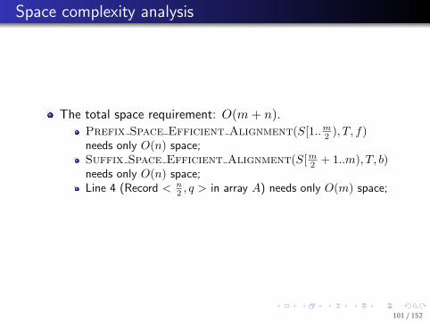
.. Space complexity analysis
The total space requirement: O(m+ n).
Prefix Space Efficient Alignment(S[1..m2 ), T, f)needs only O(n) space;Suffix Space Efficient Alignment(S[m2 + 1..m), T, b)needs only O(n) space;Line 4 (Record < n
2 , q > in array A) needs only O(m) space;
101 / 152

. . . . . .
.. Time complexity analysis
.Theorem........Algorithm Linear Space Alignment( S, T ) still takes O(mn) time.
.Proof...
......
The algorithm implies the following recursion:T (m,n) = cmn+ T (m
2, q) + T (m
2, n− q);
Difficulty: we have no idea of q before algorithm ends; thus, the mastertheorem cannot apply directly. Guess and substitution!!!
Guess: T (m′, n′) ≤ km′n′ follows for any m′ < m and n′ < n.
Substitution:
T (m,n) = cmn+ T (m
2, q) + T (
m
2, n− q) (7)
≤ cmn+ kqm
2+ k(n− q)
m
2(8)
= cmn+ kqm
2+ kn
m
2− kq
m
2(9)
≤ (c+k
2)mn (10)
= kmn (set k = 2c) (11)102 / 152

. . . . . .
.
......Extended Reading 1: From global alignment to local alignment
103 / 152
. . . . . .
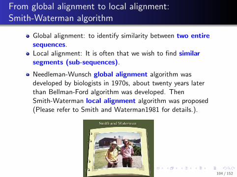
..
From global alignment to local alignment:Smith-Waterman algorithm
Global alignment: to identify similarity between two entiresequences.Local alignment: It is often that we wish to find similarsegments (sub-sequences).
Needleman-Wunsch global alignment algorithm wasdeveloped by biologists in 1970s, about twenty years laterthan Bellman-Ford algorithm was developed. ThenSmith-Waterman local alignment algorithm was proposed(Please refer to Smith and Waterman1981 for details.).
104 / 152

. . . . . .
.. Local alignment vs. global alignment: two difference
The objective of local alignment is to identify similar segmentsof two sequence. The other regions can be treated asindependent and thus form “random matches”. To distinguishrandom matches and true matches, the scoring schema wasdesigned to assign random matches with negative expectedscore, i.e., ∑
a,b
qaqbs(a, b) < 0
The recursion was changed by adding an extra possibility:
OPT (i, j) = max
0s(Si, Tj) +OPT (i− 1, j − 1)s(‘ ′, Tj) +OPT (i, j − 1)s(Si, ‘
′) +OPT (i− 1, j)Taking the option 0 corresponds to starting a new alignment:if we obtain a negative score for OPT (i, j), this means thatthe subsequences S[1..i] and T [1..j] are independent. Thus, itis better to start a new alignment rather than extend the oldone. 105 / 152

. . . . . .
.. An example
Note that the consequence of the 0 option is that the top rowand left column are set as 0.
106 / 152

. . . . . .
.. Local alignment vs. global alignment: two difference
As the local alignment aims to represent similar segments, itcan end at any cell in the matrix. Thus, instead of taking thebottom-right corner in global alignment, we look for thehighest value in the matrix and start backtracking from there.The backtrack ends when we meets a cell with value 0, whichcorresponds to the start of an alignment.
107 / 152

. . . . . .
.
......Extended Reading 2: How to derive a reasonable scoring schema?
108 / 152

. . . . . .
..
Profile-HMM: a generative model of multiple-sequencealignment
109 / 152

. . . . . .
..
PAM250: one of the most popular substitution matrices inBioinformatics
Please refer to “PAM matrix for Blast algorithm” (by C.Alexander, 2002) for the details to calculate PAM matrix.
110 / 152
. . . . . .
.
......
Extended Reading 3: How to measure the significance of analignment?
111 / 152

. . . . . .
.. Measure the significance of a segment pair
When two random sequences of length m and n are compared,the probability of finding a pair of segments with a scoregreater than or equal to S is 1− e−y, where y = Kmne−λS .
Please refer to Altschul1990 for details.
112 / 152

. . . . . .
.
......
Extended Reading 4: An FPGA implementation ofSmith-Waterman algorithm
113 / 152

. . . . . .
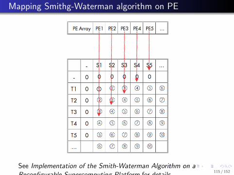
.. The potential parallelity of SmithWaterman algorithm
For example, in the first cycle, only one element marked as (1)could be calculated. In the second cycle, two elements marked as(2) could be calculated. In the third cycle, three elements markedas (3) could be calculated, etc., and this feature implies that thealgorithm has a very good potential parallelity.
114 / 152
. . . . . .
.. Mapping Smithg-Waterman algorithm on PE
See Implementation of the Smith-Waterman Algorithm on aReconfigurable Supercomputing Platform for details.
115 / 152

. . . . . .
.. PE design of a card for Dawning 4000L
116 / 152

. . . . . .
.. Smith-Waterman card for Dawning 4000L
117 / 152

. . . . . .
.. Performance of Dawning 4000L
2
2Some pictures were excerpted from Introduction to algorithms118 / 152

. . . . . .
.
......Bellman-Held-Karp for TSP problem: recursion over graphs
119 / 152

. . . . . .
.. Travelling Salesman Problem
.
......
INPUT: a list of n cities (denoted as V ), and the distancesbetween each pair of cities dij (1 ≤ i, j ≤ n);OUTPUT: the shortest tour that visits each city exactly once andreturns to the origin city
..1.
2
.
3
. 4.
1
.3
.
5
.
3
.
8
.
7
#Tours: 6
Tour 1: 1 → 2 → 3 → 4 → 1 (12)Tour 2: 1 → 2 → 4 → 3 → 1 (21)Tour 3: 1 → 3 → 2 → 4 → 1 (23)....
120 / 152

. . . . . .
.. Consider a tightly related problem
.Definition..
......
s(S, e) = the minimum distance, starting from city 1, visiting allcities in S, and finishing at city e ∈ S.
..1.
2
.
3
. 4.
1
.3
.
5
.
3
.
8
.
7
It suffices to calculate s(S, e) for any S ∈ {1, 2, ..., n} and citye since:
There are 3 cases of the city from which we return to 1.Thus, the shortest tour can be calculated as:min{D({1, 2, 3, 4}, 2) + d2,1,D({1, 2, 3, 4}, 3) + d3,1,D({1, 2, 3, 4}, 4) + d4,1}
121 / 152

. . . . . .
.. Let’s start from the smallest problem
It is trivial to calculate D(S, e) when S consists of only 1cities.
..1.
2
.
3
.
1
.
5
.
8
..
D({2}, 2) = d12;
D({3}, 3) = d13;
But how to solve a large problem, say D({2, 3, 4}, 4)?
122 / 152

. . . . . .
.. Divide a larger problem into smaller problems
..1.
2
.
3
. 4.
1
.3
.
5
.
3
.
8
.
7
.... 1.
2
.
3
. 4.
1
.3
.
5
.
3
.
8
.
7
...
D({2, 3, 4}, 4) = min{D({2, 3}, 3) + d34, D({2, 3}, 2) + d24};Optimal substructure property:
s(S, e) =
{d1e if S = {e}minm∈S−{e}(D(S − {e},m) + dme) otherwise
123 / 152

. . . . . .
.. Bellman-Held-Karp algorithm [1962]
function s(S, e)
1: if S = {e} then2: return d1e;3: end if4: d = ∞;5: for all city m ∈ S, and m ̸= e do6: if D(S − {e},m) + dme < d then7: d = D(S − {e},m) + dme;8: end if9: end for
10: return d;
Space complexity:∑n−1
k=2 k(n−1k
)+ n− 1 = (n− 1)2n−2
Time complexity:∑n−1
k=2 k(k − 1)(n−1k
)+ n− 1 = O(2nn2).
124 / 152

. . . . . .
.
......SingleSourceShortestPath problem: recursion over graphs
125 / 152

. . . . . .
.. SingleSourceShortestPath problem
.
......
INPUT:A directed graph G =< V,E >. Each edge e = (u, v) has a weightor distance d(u, v). Two special nodes: source s, and destination t;OUTPUT:A shortest path from s to t; that is, the sum weight of the edges isminimized.
..s.
u
.
v
.
t
.
w
.5
.
5
.
6
.4
.
3
.
6
. 2. 1. 2. 7
126 / 152

. . . . . .
.. ShortestPath problem: cycles
..s.
a
. c.
e
.
b
. d.
f
. t.3
.5
.
2
.
−4
.4
.8
.
7
. 6.
3
.-3
.
-6
.0.
3
.5
.
−∞
.
−∞
.−∞
.
-1
.11
Here d(i, j) might be negative; however, there should be nonegative cycle, i.e. the sum weight of edges in any cycleshould be greater than 0.In fact, a negative cycle means an −∞ shortest-path weight.Since e and f form a negative-weight cycle reachable from s,they have shortest-path weight of −∞ from s.
127 / 152

. . . . . .
.
......
Trial 1: describing the sub-problem as finding the shortest path ina graph
128 / 152

. . . . . .
.. Trial 1: recursion over graphs
Solution: a path. Describe the solving process as series ofdecisions. At each decision stage, we need to determine anedge to the subsequent node.
Suppose we have already worked out the optimal solution O.
Consider the first decision in O. The options are:
All edges starting from s: Suppose we use an edge (s, v).Then it suffices to calculate the shortest path in graphG′ =< V ′, E′ >, where node s and related edges are removed.
Thus, the original problem can be reduced into smallersub-problems.
General form of sub-problem: to find the shortest path fromnode v to t in graph G.
129 / 152
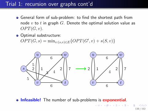
. . . . . .
.. Trial 1: recursion over graphs cont’d
General form of sub-problem: to find the shortest path fromnode v to t in graph G. Denote the optimal solution value asOPT (G, v).
Optimal substructure:OPT (G, s) = minv:(s,v)∈E{OPT (G′, v) + s(S, v)}
..s.
u
.
v
.
t
.
w
.5
.
5
.
6
.4
.3
.
6
. 2. 1. 2. 7.
u
.
v
.
t
.
w
.
6
.4
.
6
. 2. 1. 2. 7
Infeasible! The number of sub-problems is exponential.
130 / 152

. . . . . .
.
......Trial 2: another problem form with a new variable
131 / 152

. . . . . .
..
Trial 2: simplifying sub-problem form via limiting pathlength
Solution: the shortest path from node s to t is a path with at mostn nodes (Why? no negative cycle ⇒ removing cycles in a path canshorten the path). Let’s describe the solving process as a process ofmultiple-stage decisions; at each decision stage, we decide thesubsequent node from current node.
Suppose we have already worked out the optimal solution O.
Consider the first decision in O. The feasible options are:
All adjacent nodes of s: Suppose we choose an edge (s, v) tonode v. Then the left-over is to find the shortest path from vto t via at most n− 2 edges.
Thus the general form of subproblem can be designed as: to findthe shortest path from node v to t with at most k edges(k ≤ n− 1). Denote the optimal solution value as OPT (v, k).
Optimal substructure:
OPT [v, k] = min
{OPT [v, k − 1],
min(v,w)∈E{OPT [w, k − 1] + d(v, w)}
Note: the first item OPT (v, k − 1) is introduced to express “atmost”.
132 / 152

. . . . . .
.. Bellman-Ford algorithm [1956, 1958]
Bellman Ford(G, s, t)
1: for any node v ∈ V do2: OPT [v, 0] = ∞;3: end for4: for k = 0 to n− 1 do5: OPT [t, k] = 0;6: end for7: for k = 1 to n− 1 do8: for all node v (in an arbitrary order) do
9: OPT [v, k] = min
{OPT [v, k − 1]
min(v,w)∈E{OPT [w, k − 1] + d(v, w)}10: end for11: end for12: return OPT [s, n− 1];
Note that the algorithm actually finds the shortest path from everypossible source to t (or from s to every possible destination).
133 / 152

. . . . . .
.. Richard Bellman
See ”Richard Bellman on the birth of dynamic programming” (S.Dreyfus, 2002) and ”On the routing problem” (R. Bellman, 1958)for details.
134 / 152

. . . . . .
.. An example
..b.
s
.
c
.
e
.
d
. t.
−4
.
6
. 4.
2
. −2
.
−1
.
−3
.
8
.
−3
.
3
Source node k = 0 k = 1 k = 2 k = 3 k = 4 k = 5
t 0 0 0 0 0 0
s - -3 -3 -4 -6 -6
b - - 0 -2 -2 -2
c - 3 3 3 3 3
d - 4 3 3 2 0
e - 2 0 0 0 0
135 / 152

. . . . . .
.. Shortest path tree
..b.
s
.
c
.
e
.
d
. t.
−4
.
6
. 4.
2
. −2
.
−1
.
−3
.
8
.
−3
.
3
Source node k = 0 k = 1 k = 2 k = 3 k = 4 k = 5
t 0 0 0 0 0 0
s - -3 -3 -4 -6 -6
b - - 0 -2 -2 -2
c - 3 3 3 3 3
d - 4 3 3 2 0
e - 2 0 0 0 0
Note: the shortest paths from all nodes to t form a shortest pathtree. 136 / 152

. . . . . .
.. Time complexity
...1 Cursory analysis: O(n3). (There are n2 subproblems, and foreach subproblem, we need at most O(n) operations in line 7.
...2 Better analysis: O(mn). (Efficient for sparse graph, i.e.m << n2.)
For each node v, line 7 need O(dv) operations, where dvdenotes the degree of node v;Thus the inner for loop (lines 6-8) needs
∑v dv = O(m)
operations;Thus the outer for loop (lines 5-9) needs O(nm) operations.
137 / 152

. . . . . .
.
......Extension: detecting negative cycle
138 / 152

. . . . . .
.Theorem..
......
If t is reachable from node v, and v is contained in a negativecycle, then we have: limk→∞OPT (v, k) = −∞.
..b.
s
.
c
.
e
. t.
−4
.
0
.
−2
. 0.
4
.
−3
.
0
.
0
Intuition: a traveling of the negative cycle leads to a shorterlength. Say,length(b → t) = 0length(b → e → c → b → t) = −1length(b → e → c → b → e → c → b → t) = −2· · · · · · 139 / 152

. . . . . .
.Corollary..
......
If there is no negative cycle in G, then for all node v, and k ≥ n,OPT (v, k) = OPT (v, n).
Source node k=0 k=1 k=2 k=3 k=4 k=5 k=6 k=7 k=8 k=9 k=10 k=11
t 0 0 0 0 0 0 0 0 0 0 0 0
s - -3 -3 -4 -6 -6 -6 -6 -6 -6 -6 -6
b - - 0 -2 -2 -2 -2 -2 -2 -2 -2 -2
c - 3 3 3 3 3 3 3 3 3 3 3
d - 4 3 3 2 0 0 0 0 0 0 0
e - 2 0 0 0 0 0 0 0 0 0 0
..b.
s
.
c
.
e
.
d
. t.
−4
.
6
. 4.
2
. −2
.
−1
.
−3
.
8
.
−3
.
3140 / 152

. . . . . .
.. Detecting negative cycle via adding edges and a node t
Expanding G to G′ to guarantee that t is reachable from thenegative cycle:
...1 Adding a new node t;
...2 For each node v, adding a new edge (v, t) with d(v, t) = 0;
Property: G has a negative cycle C (say, b → e → c → b) ⇒t is reachable from a node in C. Thus, the above theoremapplies.
..b .
s
.
c
.
e
.
−4
.
−2
.
4
.
−3
.b.
s
.
c
.
e
. t.
−4
.
0
.
−2
. 0.
4
.
−3
.
0
.
0
141 / 152

. . . . . .
.. An example of negative cycle
..b.
s
.
c
.
e
. t.
−4
.
0
.
−2
. 0.
4
.
−3
.
0
.
0
Source node k=0 k=1 k=2 k=3 k=4 k=5 k=6 k=7 k=8 · · ·t 0 0 0 0 0 0 0 0 0 · · ·s - 0 -4 -6 -9 -9 -11 -11 -12 · · ·b - 0 -2 -5 -5 -7 -7 -8 -8 · · ·c - 0 0 0 -2 -3 -3 -3 -4 · · ·e - 0 -3 -3 -5 -5 -6 -6 -6 · · ·
142 / 152

. . . . . .
.
......Application of Bellman-Ford algorithm: Internet router protocol
143 / 152

. . . . . .
.. Internet router protocol
Problem statement:
Each node denotes a route, and the weight denotes thetransmission delay of the link from router i to j.
The objective to design a protocol to determine the quickestroute when router s wants to send a package to t.
144 / 152

. . . . . .
..
Internet router protocol: Dijkstra’s algo vs. Bellman-Fordalgo
Choice: Dijkstra algorithm.
However, the algorithm needs global knowledge, i.e. theknowledge of the whole graph, which is (almost) impossible toobtain.
In contrast, the Bellman-Ford algorithm needs only localinformation, i.e. the information of its neighboorhoodrather than the whole network.
145 / 152

. . . . . .
.. Application: Internet router protocol
AsynchronousShortestPath(G, s, t)
1: Initially, set OPT [t, t] = 0, and OPT [v, t] = ∞;2: Label node t as “active”; //Here a node v is called “active” if
OPT [v, t] has been changed;3: while exists an active node do4: Select an active node w arbitrarily;5: Remove w’s “active” label;6: for all edges (v, w) (in an arbitrary order) do
7: OPT [v, t] = min
{OPT [v, t]
OPT [w, t] + d(v, w)
8: if OPT [v, t] was updated then9: Label v as ”active”;
10: end if11: end for12: end while
146 / 152

. . . . . .
.
......A related problem: LongestPath problem
147 / 152

. . . . . .
.. LongestPath problem
.
......
INPUT:A directed graph G =< V,E >. Each edge (u, v) has a distanced(u, v). Two nodes s and t.OUTPUT:The longest simple path from s to t.
..q. r.
s
.
t
Hardness: LongestPath problem is NP-hard. (Hint: it is obviousthat LongestPath problem contains HamiltonianPath as itsspecial case. )
148 / 152
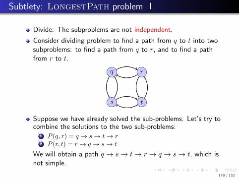
. . . . . .
.. Subtlety: LongestPath problem I
Divide: The subproblems are not independent.
Consider dividing problem to find a path from q to t into twosubproblems: to find a path from q to r, and to find a pathfrom r to t.
..q. r.
s
.
t
Suppose we have already solved the sub-problems. Let’s try tocombine the solutions to the two sub-problems:
...1 P (q, r) = q → s → t → r
...2 P (r, t) = r → q → s → t
We will obtain a path q → s → t → r → q → s → t, which isnot simple.
149 / 152

. . . . . .
.. Subtlety: LongestPath problem II
In other words, the use of s in the first subproblem preventsus from using s in the second subproblem. However, wecannot obtain the optimal solution to the second subproblemwithout using s.
150 / 152

. . . . . .
.. LongestPath versus ShortestPath
In contrast, the ShortestPath problem does not have thisdifficulty.
Why? The solutions to the subproblems share no node.Suppose the shortest paths P (q, r) and P (r, t) share a nodew(w ̸= r). Then there will be a cyclew → · · · → r → · · · → w. Removing this cycle leads to ashorter path (no negative cycle). A contradiction.
This means that the two subproblems are independent: thesolution of one subproblem does not affect the solution toanother subproblem.
151 / 152

. . . . . .
.
......
A greedy algorithm exists when posing a stricter limit, i.e., alledges have a positive weight.
We will talk about this in next lectures.
152 / 152


![Introduction to Algorithm Analysis - Nanjing Universitycs.nju.edu.cn/algorithm/slides/01.pdfIntroduction to Algorithm Analysis Algorithm : Design & Analysis [1] As soon as an Analytical](https://img.dokumen.tips/doc/110x75/5b336a807f8b9adf6c8cd516/introduction-to-algorithm-analysis-nanjing-to-algorithm-analysis-algorithm-design.jpg)


![Fundamentals of Algorithm Analysis Algorithm : Design & Analysis [Tutorial - 1]](https://img.dokumen.tips/doc/110x75/5a4d1b527f8b9ab0599a8161/fundamentals-of-algorithm-analysis-algorithm-design-analysis-tutorial.jpg)


