Embed Size (px)
Citation preview

...
.
...
.
...
.
...
.
...
.
...
.
...
.
...
.
...
.
...
.
CS711008Z Algorithm Design and AnalysisLecture 7. Basic algorithm design technique: Greedy
Dongbo Bu
Institute of Computing TechnologyChinese Academy of Sciences, Beijing, China
1 / 192

...
.
...
.
...
.
...
.
...
.
...
.
...
.
...
.
...
.
...
.
Outline
Greedy is usually used to maximize or minimize a set functionf(S), where S is a subset of a ground set.Two examples to exhibit the connection with dynamicprogramming: SingleSourceShortestPath problem andIntervalScheduling problem.Elements of greedy technique.Other examples: Huffman Code, Spanning Tree.Theoretical foundation of greedy technique: Matroid andsubmodular set functions.Important data structures: Binomial Heap, FibonacciHeap, Union-Find.
2 / 192

...
.
...
.
...
.
...
.
...
.
...
.
...
.
...
.
...
.
...
.
Greedy techniqueGreedy technique typically applies to the optimizationproblems if:
1 The original problem can be divided into smaller subproblems.2 The recursion among sub-problems can be represented as
optimal-substructure property: the optimal solution to theoriginal problem can be calculated through combining theoptimal solutions to subproblems.
3 We can design a greedy-selection rule to select a certainsub-problem at a stage.
In particular, greedy is usually used to solve an optimizationproblem whose solving process can be described as amultistage decision process, e.g., solution has the formX = [x1, x2, ..., xn], xi = 0/1.For this type of problems, we can construct a tree toenumerate all possible decisions, and greedy technique canbe treated as finding a set of paths from root (null solution)to a leaf node (complete solution). At each intermediatenode, greedy rule is applied to select one of its children nodes.
3 / 192

...
.
...
.
...
.
...
.
...
.
...
.
...
.
...
.
...
.
...
.
The first example: Two versions of IntervalSchedulingproblem
4 / 192

...
.
...
.
...
.
...
.
...
.
...
.
...
.
...
.
...
.
...
.
IntervalScheduling problem
Practical problem:A class room is requested by several courses;The i-th course Ai starts from Si and ends at Fi.
Objective: to meet as many students as possible.
5 / 192

...
.
...
.
...
.
...
.
...
.
...
.
...
.
...
.
...
.
...
.
An instance
A2 A4 A7 A8
A1 A3 A5 A9
A6
W2 = 5 W4 = 2 W7 = 1 W8 = 3
W1 = 1 W3 = 4 W5 = 3 W9 = 5
W6 = 2
Time
Solutions: S1 = {A1,A3,A5,A8} | S2 = {A6,A9}Benefits: B(S1) = 1 + 4 + 3 + 3 = 11 | B(S2) = 2 + 5 = 7
6 / 192

...
.
...
.
...
.
...
.
...
.
...
.
...
.
...
.
...
.
...
.
IntervalScheduling problem: version 1
INPUT:n activities A = {A1,A2, ...,An} that wish to use a resource. Eachactivity Ai uses the resource during interval [Si,Fi). The selectionof activity Ai yields a benefit of Wi.OUTPUT:To select a collection of compatible activities to maximizebenefits.
Here, Ai and Aj are compatible if there is no overlap betweenthe corresponding intervals [Si,Fi) and [Sj,Fj), i.e. theresource cannot be used by more than one activities at a time.It is assumed that the activities have been sorted according tothe finishing time, i.e. Fi ≤ Fj for any i < j.
7 / 192

...
.
...
.
...
.
...
.
...
.
...
.
...
.
...
.
...
.
...
.
Defining general form of subproblems I
It is not easy to solve a problem with n activities directly.Let’s see whether it can be reduced into smaller sub-problems.Solution: a subset of activities. Let’s describe the solvingprocess as a series of decisions: at each decision step, anactivity was chosen to use the resource.Suppose we have already worked out the optimal solution.Consider the first decision in the optimal solution, i.e.whether An is selected or not. There are 2 options:
1 Select activity An: the selection leads to a smallersubproblem, namely selecting from the activities endingbefore Sn.
A2 A4 A7 A8
A1 A3 A5 A9
A6
W2 = 5 W4 = 2 W7 = 1 W8 = 3
W1 = 1 W3 = 4 W5 = 3 W9 = 5
W6 = 2
Time
8 / 192

...
.
...
.
...
.
...
.
...
.
...
.
...
.
...
.
...
.
...
.
Defining general form of subproblems II
2 Abandon activity An: then it suffices to solve another smallersubproblem: to select activities from A1,A2, ...,An−1.
A2 A4 A7 A8
A1 A3 A5 A9
A6
W2 = 5 W4 = 2 W7 = 1 W8 = 3
W1 = 1 W3 = 4 W5 = 3 W9 = 5
W6 = 2
Time
9 / 192

...
.
...
.
...
.
...
.
...
.
...
.
...
.
...
.
...
.
...
.
Optimal sub-structure property
Summarizing the two cases, we can design the general form ofsubproblems as: selecting a collection of activities fromA1,A2, ...,Ai to maximize benefits. Let’s denote theoptimal solution value as OPT(i).Optimal substructure property: (“cut-and-paste” argument)
OPT(i) = max
{OPT(pre(i)) + Wi
OPT(i − 1)
Here, pre(i) denotes the largest index of the activities endingbefore Si.
10 / 192

...
.
...
.
...
.
...
.
...
.
...
.
...
.
...
.
...
.
...
.
Dynamic programming algorithm
Recursive_DP(i)Require: All Ai have been sorted in the increasing order of Fi.1: if i ≤ 0 then2: return 0;3: end if4: if i == 1 then5: return W1;6: end if7: Let pre(i) denotes the largest index of the activities ending before Si
8: m = max
{Recursive_DP(pre(i)) + Wi
Recursive_DP(i − 1)9: return m;
The original problem can be solved by callingRecursive_DP(n).It needs O(n log n) to sort the activities and determine pre(.),and the dynamic programming needs O(n) time. Thus, thetotal running time is O(n log n)
11 / 192

...
.
...
.
...
.
...
.
...
.
...
.
...
.
...
.
...
.
...
.
multistage decision process
P0 : X = [?, ?, ?, ?, ?, ?, ?, ?, ?]
P1 : X = [?, ?, ?, ?, ?, ?, ?, ?, 1] P2 : X = [?, ?, ?, ?, ?, ?, ?, ?, 0]
x9 = 1 x9 = 0
Here we represent a solution as X = [x1, x2, ..., x9], wherexi = 1 denotes the selection of activity Ai and abandonotherwise.At the first decision step, we have to enumerate both optionsx9 = 0 and x9 = 1 as we have no idea which one is optimal.
12 / 192

...
.
...
.
...
.
...
.
...
.
...
.
...
.
...
.
...
.
...
.
A more cumbersome dynamic programming algorithm
It is not easy to solve a problem with n activities directly.Let’s see whether it can be reduced into smaller sub-problems.Solution: a subset of activities. Let’s describe the solvingprocess as a series of decisions: at each decision step, anactivity is chosen to use the resource.Suppose we have already worked out the optimal solution.Consider the first decision in the optimal solution, i.e. acertain activity Ai is selected. There are at most n options:
Select an activity Ai: the selection leads to a smallersubproblem, namely, selecting from the activity set with Aiand the activities conflicting with Ai removed.
A2 A4 A7 A8
A1 A3 A5 A9
A6
W2 = 5 W4 = 2 W7 = 1 W8 = 3
W1 = 1 W3 = 4 W5 = 3 W9 = 5
W6 = 2
Time
13 / 192

...
.
...
.
...
.
...
.
...
.
...
.
...
.
...
.
...
.
...
.
Optimal sub-structure property
Summarizing these cases, we can design the general form ofsubproblems as: selecting a collection of activities from asubset S (S ⊆ {A1,A2, ...,An}) to maximize benefits.Let’s denote the optimal solution value as OPT(S).Optimal substructure property: (“cut-and-paste” argument)
OPT(S) = maxAi∈S
{OPT(R(S,Ai)) + Wi}
Here, R(S,Ai) represents the subset with Ai and the activitiesconflicting with Ai removed from S.
14 / 192

...
.
...
.
...
.
...
.
...
.
...
.
...
.
...
.
...
.
...
.
Dynamic programming algorithm
Recursive_DP(S)1: if S is empty then2: return 0;3: end if4: m = 0;5: for all activity Ai ∈ S do6: Set S′ as the subset with Ai and the activities conflicting with Ai
removed from S;7: if m <Recursive_DP(S′) + Wi then8: m = Recursive_DP(S′) + Wi;9: end if
10: end for11: return m;
The original problem can be solved by callingRecursive_DP({A1,A2, ...,An}).The total running time is O(2n) as the number ofsubproblems is exponential.
15 / 192

...
.
...
.
...
.
...
.
...
.
...
.
...
.
...
.
...
.
...
.
Multistage decision process
x1 = A1/A2/.../A9
X = [??...?]P0
X = [A1?...?]P1
X = [A2?...?]P2
......X = [A9?...?]
P9
Here we represent the optimal solution as X = [x1, x2, ......],where xi ∈ {A1,A2, ...,A9} denotes the activity selected atthe i-th decision step.At the first decision step, we have to enumerate 9 optionsx1 = A1, x1 = A2, ......, x1 = A9 as we have no idea whichone is optimal, i.e.,
OPT(S) = maxAi∈S
{OPT(R(S,Ai)) + Wi}.
16 / 192

...
.
...
.
...
.
...
.
...
.
...
.
...
.
...
.
...
.
...
.
IntervalScheduling problem: version 2
17 / 192
...
.
...
.
...
.
...
.
...
.
...
.
...
.
...
.
...
.
...
.
Let’s investigate a special case
A2 A4 A7 A8
A1 A3 A5 A9
A6
W2 = 1 W4 = 1 W7 = 1 W8 = 1
W1 = 1 W3 = 1 W5 = 1 W9 = 1
W6 = 1
Time
A special case of IntervalScheduling problem with allweights wi = 1.
18 / 192

...
.
...
.
...
.
...
.
...
.
...
.
...
.
...
.
...
.
...
.
IntervalScheduling problem: version 2
INPUT:n activities A = {A1,A2, ...,An} that wish to use a resource. Eachactivity Ai uses the resource during interval [Si,Fi).OUTPUT:To select as many compatible activities as possible.
19 / 192

...
.
...
.
...
.
...
.
...
.
...
.
...
.
...
.
...
.
...
.
Greedy-selection property
20 / 192

...
.
...
.
...
.
...
.
...
.
...
.
...
.
...
.
...
.
...
.
Another property: greedy-selection
Since this is just a special case, the optimal substructureproperty still holds.Besides the optimal substructure property, the special weightsetting leads to “greedy-selection” property, i.e., to selectas many courses as possible, we first select the course withthe earliest ending time.
TheoremSuppose A1 is the activity with the earliest ending time. A1 isused in an optimal solution.
21 / 192

...
.
...
.
...
.
...
.
...
.
...
.
...
.
...
.
...
.
...
.
Proof of the greedy-selection rule
Proof.Suppose we have an optimal solution O = {Ai1,Ai2, ...,AiT}but Ai1 = A1.A1 is compatible with Ai2, ...,AiT since A1 ends earlier thanAi1.Exchange argument: Construct a new subsetO′ = O − {Ai1} ∪ {A1}. It is clear that O′ is also an optimalsolution since |O′| = |O|.
O’A2 A4 A7 A8
A1 A3 A5 A9
A6
Time
OA2 A4 A7 A8
A1 A3 A5 A9
A6
22 / 192
...
.
...
.
...
.
...
.
...
.
...
.
...
.
...
.
...
.
...
.
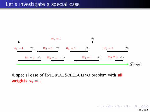
Simplifying the DP algorithm into a greedy algorithm
Interval_Scheduling_Greedy(n)Require: All Ai have been sorted in the increasing order of Fi.1: previous_finish_time = −∞;2: for i = 1 to n do3: if Si ≥ previous_finish_time then4: Select activity Ai;5: previous_finish_time = Fi;6: end if7: end for
Time complexity: O(n log n) (sorting activities in the increasingorder of finish time).
23 / 192

...
.
...
.
...
.
...
.
...
.
...
.
...
.
...
.
...
.
...
.
An example: Step 1
2 4 7 8
1 3 5 9
6
24 / 192

...
.
...
.
...
.
...
.
...
.
...
.
...
.
...
.
...
.
...
.
Step 2
2 4 7 8
1 3 5 9
6
25 / 192

...
.
...
.
...
.
...
.
...
.
...
.
...
.
...
.
...
.
...
.
Step 3
2 4 7 8
1 3 5 9
6
26 / 192
...
.
...
.
...
.
...
.
...
.
...
.
...
.
...
.
...
.
...
.
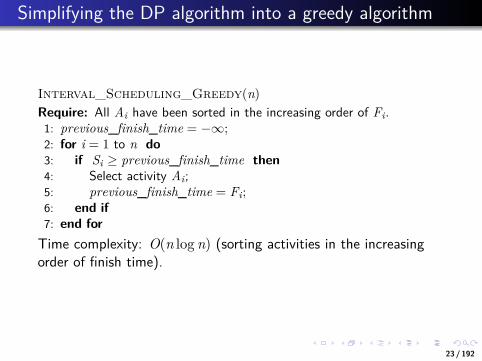
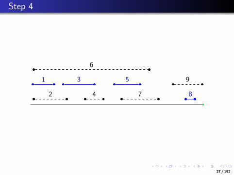
Step 4
2 4 7 8
1 3 5 9
6
27 / 192

...
.
...
.
...
.
...
.
...
.
...
.
...
.
...
.
...
.
...
.
Greedy-selection rule in multistage decision process
x1 = A1/A2/.../A9
X = [??...?]P0
X = [A1?...?]P1
X = [A2?...?]P2
...... X = [A9?...?]P9
Here we represent the optimal solution as X = [x1, x2, ......],where xi ∈ {A1,A2, ...,A9} denotes the activity selected atthe i-th decision step.At the first decision step, the dynamic programming techniquehas to enumerate 9 options x1 = A1, x1 = A2, ..., x1 = A9 asit is unknown which one is optimal, i.e.,
OPT(S) = maxAi∈S
{OPT(R(S,Ai)) + 1}
In contrast, the greedy algorithm selects A1 directly accordingto the greedy-selection property, i.e.,
OPT(S) = OPT(R(S,A1)) + 1.28 / 192

...
.
...
.
...
.
...
.
...
.
...
.
...
.
...
.
...
.
...
.
Elements of greedy algorithm
In general, greedy algorithms have five components:1 A candidate set, from which a solution is created2 A selection function, which chooses the best candidate to be
added to the solution3 A feasibility function, that is used to determine if a candidate
can be used to contribute to a solution4 An objective function, which assigns a value to a solution, or a
partial solution, and5 A solution function, which will indicate when we have
discovered a complete solution
29 / 192

...
.
...
.
...
.
...
.
...
.
...
.
...
.
...
.
...
.
...
.
DP versus Greedy
Similarities:1 Both dynamic programming and greedy techniques are
typically applied to optimization problems.2 Optimal substructure: Both dynamic programming and
greedy techniques exploit the optimal substructure property.3 Beneath every greedy algorithm, there is almost always
a more cumbersome dynamic programming solution —CRLS
30 / 192

...
.
...
.
...
.
...
.
...
.
...
.
...
.
...
.
...
.
...
.
DP versus Greedy cont’d
Differences:1 A dynamic programming method typically enumerate all
possible options at a decision step, and the decision cannotbe determined before subproblems were solved.
2 In contrast, greedy algorithm does not need to enumerate allpossible options—it simply make a locally optimal (greedy)decision without considering results of subproblems.
Note:Here, “local” means that we have already acquired part of anoptimal solution, and the partial knowledge of optimalsolution is sufficient to help us make a wise decision.Sometimes a rigorous proof is unavailable, thus extensiveexperimental results are needed to show the efficiency of thegreedy technique.
31 / 192

...
.
...
.
...
.
...
.
...
.
...
.
...
.
...
.
...
.
...
.
How to design greedy method?
Two strategies:1 Simplifying a dynamic programming method through
greedy-selection;2 Trial-and-error: Describing the solution-generating process as
making a sequence of choices, and trying differentgreedy-selection rules.
32 / 192

...
.
...
.
...
.
...
.
...
.
...
.
...
.
...
.
...
.
...
.
Trying other greedy rules
33 / 192
...
.
...
.
...
.
...
.
...
.
...
.
...
.
...
.
...
.
...
.
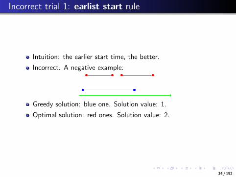
Incorrect trial 1: earlist start rule
Intuition: the earlier start time, the better.Incorrect. A negative example:
Greedy solution: blue one. Solution value: 1.Optimal solution: red ones. Solution value: 2.
34 / 192

...
.
...
.
...
.
...
.
...
.
...
.
...
.
...
.
...
.
...
.
Incorrect trial 2: trying minimal duration rule
Intuition: the shorter duration, the better.Incorrect. A negative example:
Greedy solution: blue one. Solution value: 1.Optimal solution: red ones. Solution value: 2.
35 / 192

...
.
...
.
...
.
...
.
...
.
...
.
...
.
...
.
...
.
...
.
Incorrect trial 3: trying minimal conflicts rule
Intuition: the less conflict activities, the better.Incorrect. A negative example:
Greedy solution: blue ones. Solution value: 3.Optimal solution: red ones. Solution value: 4.
36 / 192

...
.
...
.
...
.
...
.
...
.
...
.
...
.
...
.
...
.
...
.
Revisiting ShortestPath problem
37 / 192

...
.
...
.
...
.
...
.
...
.
...
.
...
.
...
.
...
.
...
.
Revisiting Single Source Shortest Paths problem
INPUT:A directed graph G =< V,E >. Each edge e =< i, j > has adistance di,j. A single source node s, and a destination node t;OUTPUT:The shortest path from s to t (Or the shortest paths from s to eachnode v ∈ V, or the shortest paths from each node v ∈ V to t).
Two versions of ShortestPath problem:1 No negative cycle: Bellman-Ford dynamic programming
algorithm;2 No negative edge: Dijkstra greedy algorithm.
38 / 192

...
.
...
.
...
.
...
.
...
.
...
.
...
.
...
.
...
.
...
.
Optimal sub-structure property in version 1
39 / 192

...
.
...
.
...
.
...
.
...
.
...
.
...
.
...
.
...
.
...
.
Optimal sub-structure propertySolution: a path from s to t with at most (n − 1) edges.Describing the solving process as a multi-stage decisionprocess: at each decision step, we decide the subsequent node.Consider the final decision (i.e. from which we reach node t).There are several possibilities for the decision:
node v such that < v, t >∈ E: then it suffices to solve asmaller subproblem, i.e. “starting from s to node v via at most(n − 2) edges”.
Thus we can design the general form of sub-problems as“starting from s to a node v via at most k edges”.Denote the optimal solution value as OPT(v, k).Optimal substructure:OPT(v, k) = min
{OPT(v, k − 1)min<u,v>∈E{OPT(u, k − 1) + du,v}
Note: the first item OPT(v, k − 1) is introduced here todescribe “at most”.Time complexity: O(mn)
40 / 192

...
.
...
.
...
.
...
.
...
.
...
.
...
.
...
.
...
.
...
.
Bellman_Ford algorithm [1956]
Bellman_Ford(G, s, t)1: for i = 0 to n do2: OPT[s, i] = 0;3: end for4: for all node v ∈ V do5: OPT[v, 0] = ∞;6: end for7: for k = 1 to n − 1 do8: for all node v (in an arbitrary order) do
9: OPT[v, k] = min
{OPT[v, k − 1],min<u,v>∈E{OPT[u, k − 1] + d(u, v)}
10: end for11: end for12: return OPT[t,n − 1];
41 / 192

...
.
...
.
...
.
...
.
...
.
...
.
...
.
...
.
...
.
...
.
An example: Step 1
s
u
v
x
t
y
1
2
4
3
1
1
2
3
2
k=0 1 2 3 4 5suvxyt
0 0 0 0 0 0
− 1
− 2
− 4
− −
− −
42 / 192

...
.
...
.
...
.
...
.
...
.
...
.
...
.
...
.
...
.
...
.
Step 2
s
u
v
x
t
y
1
2
4
3
1
1
2
3
2
k=0 1 2 3 4 5suvxyt
0 0 0 0 0 0
− 1 1
− 2 2
− 4 2
− − 4
− − 5
43 / 192

...
.
...
.
...
.
...
.
...
.
...
.
...
.
...
.
...
.
...
.
Final step
s
u
v
x
t
y
1
2
4
3
1
1
2
3
2
k=0 1 2 3 4 5suvxyt
0 0 0 0 0 0
− 1 1 1 1 1
− 2 2 2 2 2
− 4 2 2 2 2
− − 4 3 3 3
− − 5 4 4 4
Recall that the collection of the shortest paths from s to allnodes form a shortest path tree.
44 / 192

...
.
...
.
...
.
...
.
...
.
...
.
...
.
...
.
...
.
...
.
Greedy-selection property in version 2
45 / 192

...
.
...
.
...
.
...
.
...
.
...
.
...
.
...
.
...
.
...
.
Greedy-selection rule in multistage decision process
s
u
v
x
t
y
1
2
4
3
1
1
2
3
2
x1 = x/u/v
x2 = x/v/y/t
X =?????P0
x????P1
u????P2
v????P3
ux???P4
uv???P5
uy???P6
ut???P7
......
The construction of the shortest path tree rooted at s is amultistage decision process: The tree is described asX = [x1, x2, ..., x5], where xi ∈ V represents the node selectedat the i-th stage. The Dijkstra’s algorithm selects the nearestnode adjacent to “explored” nodes at each stage.This greedy-selection rule works due to the following twoobservations of Bellman_Ford algorithm, namely, someoperations are redundant, and the nearest node adjacent to“explored” nodes has its shortest distance determined. 46 / 192

...
.
...
.
...
.
...
.
...
.
...
.
...
.
...
.
...
.
...
.
Redundant calculations in Bellman_Ford algorithm
At the k-th step, let’s consider a special node v∗, the nearestnode from s via at most k − 1 edges, i.e.
OPT(v∗, k − 1) = minvOPT(v, k − 1)
Consider the optimal substructure property for v∗, i.e.
OPT(v∗, k) = min
{OPT(v∗, k − 1)min<u,v∗>∈E{OPT(u, k − 1) + du,v∗}
The above equality can be further simplified as:
OPT(v∗, k) = OPT(v∗, k − 1)
(Why? OPT(u, k − 1) ≥ OPT(v∗, k − 1) and du,v∗ ≥ 0.)
47 / 192

...
.
...
.
...
.
...
.
...
.
...
.
...
.
...
.
...
.
...
.
The meaning of OPT(v∗, k) = OPT(v∗, k − 1) for k = 2
s
u
v
x
t
y
1
2
4
3
1
1
2
3
2
k=01 2 3 4 5suvxyt
0 0 0 0 0 0
− 1 1 1 1 1
− 2
− 4
− −
− −
Intuitively v∗ (in red circles) can be treated as has alreadybeen explored using at most (k − 1) edges, and thedistance will not change afterwards. Thus, the calculations ofOPT(v∗, k) (in green rectangles) are in fact redundant.In other words, it suffices to calculateOPT[v, k] = min
{OPT[v, k − 1],min<u,v>∈E{OPT[u, k − 1] + d(u, v)}
for
the unexplored nodes v = v∗, including v, x, y, t.48 / 192
...
.
...
.
...
.
...
.
...
.
...
.
...
.
...
.
...
.
...
.
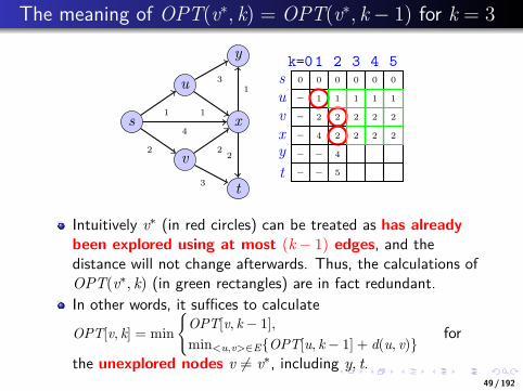
The meaning of OPT(v∗, k) = OPT(v∗, k − 1) for k = 3
s
u
v
x
t
y
1
2
4
3
1
1
2
3
2
k=01 2 3 4 5suvxyt
0 0 0 0 0 0
− 1 1 1 1 1
− 2 2 2 2 2
− 4 2 2 2 2
− − 4
− − 5
Intuitively v∗ (in red circles) can be treated as has alreadybeen explored using at most (k − 1) edges, and thedistance will not change afterwards. Thus, the calculations ofOPT(v∗, k) (in green rectangles) are in fact redundant.In other words, it suffices to calculateOPT[v, k] = min
{OPT[v, k − 1],min<u,v>∈E{OPT[u, k − 1] + d(u, v)}
for
the unexplored nodes v = v∗, including y, t.49 / 192

...
.
...
.
...
.
...
.
...
.
...
.
...
.
...
.
...
.
...
.
The meaning of OPT(v∗, k) = OPT(v∗, k − 1)
s
u
v
x
t
y
1
2
4
3
1
1
2
3
2
k=01 2 3 4 5suvxyt
0 0 0 0 0 0
− 1 1 1 1 1
− 2 2 2 2 2
− 4 2 2 2 2
− − 4 3 3 3
− − 5 4 4 4
Intuitively v∗ (in red circles) can be treated as has alreadybeen explored using at most (k − 1) edges, and thedistance will not change afterwards. Thus, the calculations ofOPT(v∗, k) (in green rectangles) are in fact redundant.In other words, it suffices to calculateOPT[v, k] = min
{OPT[v, k − 1],min<u,v>∈E{OPT[u, k − 1] + d(u, v)}
for
the unexplored nodes v = v∗ at each step.50 / 192

...
.
...
.
...
.
...
.
...
.
...
.
...
.
...
.
...
.
...
.
A faster implementation of Bellman_Ford
Fast_Bellman_Ford(G, s, t)1: S = {s}; //S denotes the set of explored nodes,2: for i = 0 to n do3: OPT[s, i] = 0;4: end for5: for all node v ∈ V do6: OPT[v, 0] = ∞;7: end for8: for k = 1 to n − 1 do9: for all node v /∈ S (in an arbitrary order) do
10: OPT[v, k] = min
{OPT[v, k − 1],min<u,v>∈E{OPT[u, k − 1] + d(u, v)}
11: end for12: Add the nodes with minimum OPT(v, k) to S;13: end for14: return OPT[t,n − 1];
51 / 192

...
.
...
.
...
.
...
.
...
.
...
.
...
.
...
.
...
.
...
.
Greedy-selection rule: select the nearest neighbor of SNow the question is how to efficiently calculate OPT(v, k) forthe unexplored nodes v /∈ S. Take the example shown below.The unexplored nodes include v, x, y and t.
s
u
v
x
t
y
1
2
4
3
1
1
2
3
2
k=01 2 3 4 5suvxyt
0 0 0 0 0 0
− 1 1 1 1 1
− 2
− 4
− −
− −
Note that it is unnecessary to consider all unexplored nodes;instead, we can consider only the unexplored nodesadjacent to an explored node, i.e., nodes v, x, y.Furthermore, among these nodes, the nearest ones (v andx) have their shortest distance determined. Thus we caniteratively select such nodes until reaching node t.
52 / 192

...
.
...
.
...
.
...
.
...
.
...
.
...
.
...
.
...
.
...
.
TheoremLet S denote the explored nodes, and for each explored node v, let d(v) denotethe shortest distance from s to v. Consider the nearest unexplored node u∗
adjacent to an explored node, i.e., u∗ is the node u (u /∈ S) that minimizesd′(u) = minw∈S{d(w) + d(w, u)}. Then the path P = s → ... → w → u∗ is oneof the shortest paths from s to u∗ with distance d′(u∗).
Proof.
Consider another path P′ from s to u∗:P′ = s → ... → x → y → ... → u∗. Let y denote the first node in P′
leaving out of S.We decompose P′ into two parts: s → ... → x → y, and y → ... → u∗.The first part should be longer. Thus, |P′| ≥ d(s, x) + d(x, y) ≥ d′(u∗).
s w
x y z
u∗
2
1 3 1 1
12 1
S : explored nodes53 / 192

...
.
...
.
...
.
...
.
...
.
...
.
...
.
...
.
...
.
...
.
Bellman_Ford vs Dijkstra: two differences1 Let v∗ denote the nearest node from s using at most k − 1 edges. The
shortest distance d(v∗) will not change afterwards.
s
u
v
x
t
y
1
2
4
3
1
1
2
3
2
k=01 2 3 4 5suvxyt
0 0 0 0 0 0
− 1 1 1 1 1
− 2
− 4
− −
− −
2 Let’s u∗ denote the nearest unexplored node adjacent to an explorednode. The shortest path from s to u∗ is determined.
s w
x y z
u∗2
13
11
12 1
S : explored nodes 54 / 192

...
.
...
.
...
.
...
.
...
.
...
.
...
.
...
.
...
.
...
.
Dijkstra’s algorithm [1959]Dijkstra(G, s, t)1: d(s) = 0; //d(u) stores upper bound of the shortest distance from s
to u;2: for all node v = s do3: d(v) = +∞;4: end for5: S = {}; // Let S be the set of explored nodes;6: while S = V do7: Select the unexplored node v∗ (v∗ /∈ S) that minimizes d(v);8: S = S ∪ {v∗};9: for all unexplored node v adjacent to an explored node do
10: d(v) = min{d(v),minu∈S{d(u) + d(u, v)}};11: end for12: end while
Lines (9 − 11) are called “relaxing”. That is, we test whether theshortest-path to v found so far can be improved by going through u,and if so, update d(v).When du,v = 1 for any edge < u, v >, the Dijkstra’s algorithmreduces to BFS, and thus can be treated as weighted BFS.
55 / 192
...
.
...
.
...
.
...
.
...
.
...
.
...
.
...
.
...
.
...
.
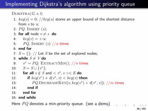
Implementing Dijkstra’s algorithm using priority queueDijkstra(G, s, t)1: key(s) = 0; //key(u) stores an upper bound of the shortest distance
from s to u;2: PQ. Insert (s);3: for all node v = s do4: key(v) = +∞5: PQ. Insert (v) //n times6: end for7: S = {}; // Let S be the set of explored nodes;8: while S = V do9: v∗ = PQ. ExtractMin(); //n times
10: S = S ∪ {v∗};11: for all v /∈ S and < v∗, v >∈ E do12: if key(v∗) + d(v∗, v) < key(v) then13: PQ.DecreaseKey(v, key(v∗) + d(v∗, v)); //m times14: end if15: end for16: end whileHere PQ denotes a min-priority queue. (see a demo)
56 / 192

...
.
...
.
...
.
...
.
...
.
...
.
...
.
...
.
...
.
...
.
Contributions by Edsger W. Dijkstra
The semaphore construct for coordinating multiple processors andprograms.The concept of self-stabilization — an alternative way to ensure thereliability of the system”A Case against the GO TO Statement”, regarded as a major steptowards the widespread deprecation of the GOTO statement and itseffective replacement by structured control constructs, such as thewhile loop....
57 / 192

...
.
...
.
...
.
...
.
...
.
...
.
...
.
...
.
...
.
...
.
ShortestPath: Bellman-Ford algorithm vs. Dijkstraalgorithm
A slight change of edge weights leads to a significant changeof algorithm design.
1 No negative cycle: an optimal path from s to v has at mostn − 1 edges; thus the optimal solution is OPT(v,n − 1). Tocalculate OPT(v,n − 1), we appeal to the following recursion:
OPT[v, k] = min
{OPT[v, k − 1],min<u,v>∈E{OPT[u, k − 1] + d(u, v)}
2 No negative edge: This stronger constraint on edge weightsimplies greedy-selection property. In particular, it isunnecessary to calculate OPT(v, i) for any explored nodev ∈ S, and for the nearest unexplored node adjacent to anexplored node, its shortest distance is determined.
58 / 192

...
.
...
.
...
.
...
.
...
.
...
.
...
.
...
.
...
.
...
.
Time complexity analysis
59 / 192

...
.
...
.
...
.
...
.
...
.
...
.
...
.
...
.
...
.
...
.
Time complexity of the Dijkstra’s algorithm
Operation Linked Binary Binomial Fibonaccilist heap heap heap
MakeHeap 1 1 1 1Insert 1 log n log n 1
ExtractMin n log n log n log nDecreaseKey 1 log n log n 1
Delete n log n log n log nUnion 1 n log n 1
FindMin n 1 log n 1Dijkstra O(n2) O(m log n) O(m log n) O(m + n log n)
The Dijkstra’s algorithm: n Insert, n ExtractMin, and mDecreaseKey.
60 / 192

...
.
...
.
...
.
...
.
...
.
...
.
...
.
...
.
...
.
...
.
Extension: can we reweigh the edges to make all weight positive?
61 / 192

...
.
...
.
...
.
...
.
...
.
...
.
...
.
...
.
...
.
...
.
Trial 1: Increasing all edge weights by the same amount
s u
v w
t1
−1
1
−1
1s u
v w
t6
4
6
4
6
Increasing all the weight by 5 changes the shortest path froms to t.Reason: Different paths might change by different amountalthough all edges change by the same mount.
62 / 192

...
.
...
.
...
.
...
.
...
.
...
.
...
.
...
.
...
.
...
.
Trial 2: Increasing an edge weight according to its two ends
For different paths starting from u to v, one of the constraintsof reweighing is to maintain the order of these paths underthe original weighting function. In other words, the change ofdistance following a path is independent of the intermediatenodes of the path. Thus, for any path u⇝ v, we representthe new distance as:
d′(u⇝ v) = d(u⇝ v) + c(u)− c(v)
where c(v) is a number associated with node v.As a special case, each edge (u, v) is reweighed as follows.
d′(u, v) = d(u, v) + c(u)− c(v)
Note another constraint is d′(u, v) ≥ 0 for any edge (u, v).How to achieve this objective?
63 / 192

...
.
...
.
...
.
...
.
...
.
...
.
...
.
...
.
...
.
...
.
Reweighing schema
Basic idea: We first add a new node s∗ and connect it to eachnode v with an edge weight d(s∗, v) = 0, d(v, s∗) = ∞. Nextwe set c(v) as dist(s∗, v), i.e., the shortest distance from s∗ tov.We can prove that for any node pair u and v,
d′(u, v) = d(u, v) + dist(u)− dist(v) ≥ 0
(Why? If d′(u, v) < 0, then d(u, v) + dist(u) < dist(v), whichis contradict to the fact that dist(v) is the shortest distance tov.)
64 / 192

...
.
...
.
...
.
...
.
...
.
...
.
...
.
...
.
...
.
...
.
Johnson algorithm for all pairs shortest path [1977]
Johnson(G)
1: Create a new node s∗;2: for all node v = s∗ do3: d(s∗, v) = 04: end for5: Run Bellman_Ford algorithm to calculate the shortest distance
from s∗ to each node v (denoted as dist(s∗, v));6: Reweighting: d′(u, v) = d(u, v) + dist(s∗, u)− dist(s∗, v)7: for all node u = s∗ do8: Run Dijkstra’s algorithm with the new weight d′ to calculate the
shortest paths from u to each node v (denoted as d∗(u, v));9: for all node v = s∗ do
10: d∗(u, v) = d∗(u, v)− dist(s∗, u) + dist(s∗, v);11: end for12: end for13: return d∗(u, v) for each node pair (u, v);Time complexity: O(mn + n2 log n).
65 / 192

...
.
...
.
...
.
...
.
...
.
...
.
...
.
...
.
...
.
...
.
Extension: data structures designed to speed up the Dijkstra’salgorithm
66 / 192

...
.
...
.
...
.
...
.
...
.
...
.
...
.
...
.
...
.
...
.
Binary heap, Binomial heap, and Fibonacci heap
Figure 1: Robert W. Floyd, Jean Vuillenmin, Robert Tarjan
(See extra slides for binary heap, binomial heap and Fibonacciheap)
67 / 192

...
.
...
.
...
.
...
.
...
.
...
.
...
.
...
.
...
.
...
.
Huffman Code
68 / 192

...
.
...
.
...
.
...
.
...
.
...
.
...
.
...
.
...
.
...
.
Compressing files
Practical problem: how to compact a file when you have theknowledge of frequency of letters?Example:
SYMBOL A B C D EFrequency 24 12 10 8 8Fixed Length Code 000 001 010 011 100 E(L) = 186Variable Length Code 00 01 10 110 111 E(L) = 140
69 / 192

...
.
...
.
...
.
...
.
...
.
...
.
...
.
...
.
...
.
...
.
Formulation
INPUT:a set of symbols S = {s1, s2, ..., sn} with its appearance frequencyP = {p1, p2, ..., pn};OUTPUT:assign each symbol with a binary code Ci to minimize the lengthexpectation
∑i pi|Ci|.
70 / 192

...
.
...
.
...
.
...
.
...
.
...
.
...
.
...
.
...
.
...
.
Requirement: prefix code I
To avoid the potential ambiguity in decoding, we require thecoding to be prefix code.
Definition (Prefix coding)A prefix coding for a symbol set S is a coding such that for anysymbols x, y ∈ S, the code C(x) is not prefix of the code C(y).
Intuition: A prefix code can be represented as a binary tree,where a leaf represents a symbol, and the path to a leafrepresents the code.Our objective: to design an optimal tree T to minimizeexpected length E(T) (the size of the compressed file).
71 / 192

...
.
...
.
...
.
...
.
...
.
...
.
...
.
...
.
...
.
...
.
Requirement: prefix code II
72 / 192
...
.
...
.
...
.
...
.
...
.
...
.
...
.
...
.
...
.
...
.
Full binary tree
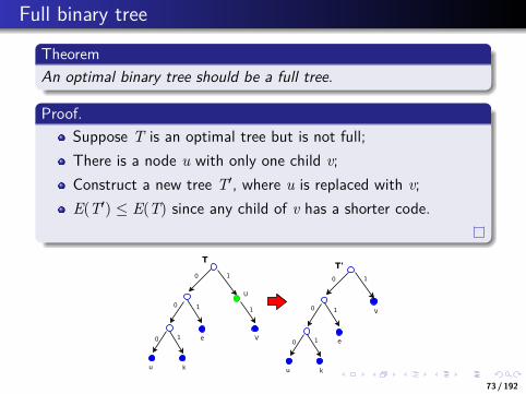
TheoremAn optimal binary tree should be a full tree.
Proof.Suppose T is an optimal tree but is not full;There is a node u with only one child v;Construct a new tree T′, where u is replaced with v;E(T′) ≤ E(T) since any child of v has a shorter code.
73 / 192

...
.
...
.
...
.
...
.
...
.
...
.
...
.
...
.
...
.
...
.
But how to construct the optimal tree?Let’s describe the solving process as a multistage decision process.
74 / 192

...
.
...
.
...
.
...
.
...
.
...
.
...
.
...
.
...
.
...
.
A top-down multiple-decision process
There a total of 2n options, which makes the dynamicprogramming infeasible.
75 / 192

...
.
...
.
...
.
...
.
...
.
...
.
...
.
...
.
...
.
...
.
Shannon-Fano coding [1949]Top-down method :
1: Sorting S in the decreasing order of frequency.2: Splitting S into two sets S1 and S2 with almost equal
frequencies.3: Recursively building trees for S1 and S2.
Figure 2: Claude Shannon and Robert Fano76 / 192

...
.
...
.
...
.
...
.
...
.
...
.
...
.
...
.
...
.
...
.
An example: Step 1
77 / 192

...
.
...
.
...
.
...
.
...
.
...
.
...
.
...
.
...
.
...
.
An example: Step 2
78 / 192

...
.
...
.
...
.
...
.
...
.
...
.
...
.
...
.
...
.
...
.
An example: Step 3
79 / 192

...
.
...
.
...
.
...
.
...
.
...
.
...
.
...
.
...
.
...
.
A bottom-up multiple-decision process
There a total of(n
2)
options.
80 / 192

...
.
...
.
...
.
...
.
...
.
...
.
...
.
...
.
...
.
...
.
Huffman code: bottom-up manner [1952]Bottom-up method:
1: repeat2: Merging the two lowest-frequency letters y and z into a new
meta-letter yz,3: Setting Pyz = Py + Pz.4: until only one label is left
81 / 192

...
.
...
.
...
.
...
.
...
.
...
.
...
.
...
.
...
.
...
.
Huffman code: bottom-up manner [1952]
Key Observations:1 In an optimal tree, depth(u) ≥ depth(v) iff Pu ≤ Pv.
(Exchange argument)2 There is an optimal tree, where the lowest-frequency letters Y
and Z are siblings. (Why?)Consider a deepest node v.v’s parent, denoted as u, should has another child, say w.w should also be a deepest node.v and w have the lowest frequency.
82 / 192

...
.
...
.
...
.
...
.
...
.
...
.
...
.
...
.
...
.
...
.
Huffman code algorithm 1952
Huffman(S,P)1: if |S| == 2 then2: return a tree with a root and two leaves;3: end if4: Extract the two lowest-frequency letters Y and Z from S;5: Set PYZ = PY + PZ;6: S = S − {Y,Z} ∪ {YZ};7: T′ =Huffman(S,P);8: T = add two children Y and Z to node YZ in T′;9: return T;
83 / 192

...
.
...
.
...
.
...
.
...
.
...
.
...
.
...
.
...
.
...
.
Example
84 / 192

...
.
...
.
...
.
...
.
...
.
...
.
...
.
...
.
...
.
...
.
Shannon-Fano vs. Huffman
85 / 192
...
.
...
.
...
.
...
.
...
.
...
.
...
.
...
.
...
.
...
.
Huffman algorithm: correctness
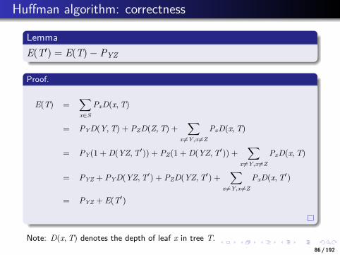
LemmaE(T′) = E(T)− PYZ
Proof.
E(T) =∑x∈S
PxD(x,T)
= PYD(Y,T) + PZD(Z,T) +∑
x=Y,x =Z
PxD(x,T)
= PY(1 + D(YZ,T′)) + PZ(1 + D(YZ,T′)) +∑
x =Y,x =Z
PxD(x,T)
= PYZ + PYD(YZ,T′) + PZD(YZ,T′) +∑
x =Y,x=Z
PxD(x,T′)
= PYZ + E(T′)
Note: D(x,T) denotes the depth of leaf x in tree T.86 / 192

...
.
...
.
...
.
...
.
...
.
...
.
...
.
...
.
...
.
...
.
Huffman algorithm: correctness cont’d
TheoremHuffman algorithm output an optimal code.
Proof.(Induction)
Suppose there is another tree t with smaller expected length;In the tree t, let’s merge the lowest frequency letters Y and Zinto a meta-letter YZ; converting t into a new tree t′ with ofsize n − 1;t′ is better than T′. Contradiction.
87 / 192

...
.
...
.
...
.
...
.
...
.
...
.
...
.
...
.
...
.
...
.
Analysis
Time complexity:T(n) = T(n − 1) + O(n) = O(n2).T(n) = T(n− 1)+O(log n) = O(n log n) if use priority queue.
Note: Huffman code is a bit different example of greedytechnique—the problem is shrinked at each step; in addition, theproblem is changed a little (the frequency of a new meta letter isthe sum frequency of its members).
88 / 192

...
.
...
.
...
.
...
.
...
.
...
.
...
.
...
.
...
.
...
.
Application
In practical operation Shannon-Fano coding is not of largerimportance. This is especially caused by the lower codeefficiency in comparison to Huffman coding.Huffman codes are part of several data formats as ZIP, GZIPand JPEG. Normally the coding is preceded by proceduresadapted to the particular contents. For example thewide-spread DEFLATE algorithm as used in GZIP or ZIPpreviously processes the dictionary based LZ77 compression.
See http://www.binaryessence.com/dct/en000003.htm for details.
89 / 192

...
.
...
.
...
.
...
.
...
.
...
.
...
.
...
.
...
.
...
.
Theoretical foundation of greedy strategy: Matroid andsubmodular functions
90 / 192

...
.
...
.
...
.
...
.
...
.
...
.
...
.
...
.
...
.
...
.
Theoretical foundation of greedy strategy
Consider the following optimization problem: given a finite setof objects N, the objective is to find a subset S ∈ F such thata set function f(S) is maximized, i.e.,
max f(S)s.t. S ∈ F
Here, F ⊆ 2N represents certain constraints over S.In general cases, the problem is clearly intractable — youwould better check all possible subsets in F to avoid missingthe optimal solution. However, in certain special cases, greedystrategy applies and generates optimal solution or goodapproximation solutions.
91 / 192

...
.
...
.
...
.
...
.
...
.
...
.
...
.
...
.
...
.
...
.
When greedy strategy is perfect or good enough?
So what conditions on either F or f(S) or both does greedystrategy needs?
Matroid: Greedy strategy generates optimal solution when f(S)is a linear function, and F can be characterized asindependent subsets.Submodular functions: Greedy strategy might generateprovably good approximation when f(S) is a submodularfunction.
92 / 192

...
.
...
.
...
.
...
.
...
.
...
.
...
.
...
.
...
.
...
.
When greedy strategy is perfect: Maximizing/minimizing a linearfunction under matroid constraint
93 / 192

...
.
...
.
...
.
...
.
...
.
...
.
...
.
...
.
...
.
...
.
Revisiting Maximal Linearly Independent Setproblem
Question: Given a set of vectors, to determine the maximallinearly independent set.Example:
V1 = [ 1 2 3 4 5 ]V2 = [ 1 4 9 16 25 ]V3 = [ 1 8 27 64 125 ]V4 = [ 1 16 81 256 625 ]V5 = [ 2 6 12 20 30 ]
Independent vector set: {V1,V2,V3,V4}
94 / 192

...
.
...
.
...
.
...
.
...
.
...
.
...
.
...
.
...
.
...
.
Calculating maximal number of independent vectors
IndependentSet(M)
1: S = {};2: for all row vector v do3: if S ∪ {v} is still independent then4: S = S ∪ {v};5: end if6: end for7: return S;
Here we adopt the independence oracle model for M:given S ⊆ N, the oracle returns whether S is independent ornot.
95 / 192

...
.
...
.
...
.
...
.
...
.
...
.
...
.
...
.
...
.
...
.
Correctness: Properties of linear independence vector setLet’s consider the linear independence for vectors.
1 Hereditary property: if B is an independent vector set andA ⊂ B, then A is also an independent vector set.
2 Augmentation property: if both A and B are independentvector sets, and |A| < |B|, then there is a vector v ∈ B − Asuch that A ∪ {v} is still an independent vector set.
Example:
V1 = [ 1 2 3 4 5 ]V2 = [ 1 4 9 16 25 ]V3 = [ 1 8 27 64 125 ]V4 = [ 1 16 81 256 625 ]V5 = [ 2 6 12 20 30 ]
Independent vector sets: A = {V1,V3,V5},B = {V1,V2,V3,V4}, and |A| < |B|.Augmentation of A: A ∪ {V4} is also independent.
96 / 192

...
.
...
.
...
.
...
.
...
.
...
.
...
.
...
.
...
.
...
.
An extension to weighted vectors
Question: Given a matrix, where each row vector isassociated with a weight, to determine a set of linearlyindependent vectors to maximize the sum of weight.Example:
V1 = [ 1 2 3 4 5 ] W1 = 9V2 = [ 1 4 9 16 25 ] W2 = 7V3 = [ 1 8 27 64 125 ] W3 = 5V4 = [ 1 16 81 256 625 ] W4 = 3V5 = [ 2 6 12 20 30 ] W5 = 1
97 / 192

...
.
...
.
...
.
...
.
...
.
...
.
...
.
...
.
...
.
...
.
Greedy-selection property
TheoremLet v be the vector with the largest weight and {v} is independent,then there is an optimal vector set A of M and A contains v.
Proof.Assume there is an optimal subset B but v /∈ B.Then we can construct A from B as follows:
1 Initially: A = {v};2 Until |A| = |B|, repeatedly find a new element of B that can
be added to A while preserving the independence of A (byaugmentation property);
Finally we have A = B − {v′} ∪ {v}.We have W(A) ≥ W(B) since W(v) ≥ W(v′) for any v′ ∈ B.A contradiction.
98 / 192

...
.
...
.
...
.
...
.
...
.
...
.
...
.
...
.
...
.
...
.
A general greedy algorithm (by Jack Edmonds [1971])
MatroidGreedy(M,W)
1: S = {};2: Sort row vectors in the decreasing order of their weights;3: for all row vector v do4: if S ∪ {v} is still independent then5: S = S ∪ {v};6: end if7: end for8: return S;
Time complexity: O(n log n + nC(n)), where C(n) is the timeneeded to query the independence oracle.
99 / 192

...
.
...
.
...
.
...
.
...
.
...
.
...
.
...
.
...
.
...
.
An extension of linear independence for vectors: matroid
100 / 192

...
.
...
.
...
.
...
.
...
.
...
.
...
.
...
.
...
.
...
.
Matroid [Haussler Whitney, 1935]
Matroid was proposed to capture the concept of linearindependence in matrix theory, and generalize the concept inother field, say graph theory.In fact, in the paper On the abstract properties of linearindependence, Haussler Whitney said:This paper has a close connection with a paper by the authoron linear graphs; we say a subgraph of a graph isindependent if it contains no circuit.
101 / 192

...
.
...
.
...
.
...
.
...
.
...
.
...
.
...
.
...
.
...
.
Origin 1 of matroid: linear independence for vectors
Let’s consider the linear independence for vectors.1 Hereditary property: if B is an independent vector set and
A ⊂ B, then A is also an independent vector set2 Augmentation property: if both A and B are independent
vector sets, and |A| < |B|, then there is a vector v ∈ B − Asuch that A ∪ {v} is still an independent vector set
Example:V1 = [ 1 2 3 4 5 ]V2 = [ 1 4 9 16 25 ]V3 = [ 1 8 27 64 125 ]V4 = [ 1 16 81 256 625 ]V5 = [ 2 6 12 20 30 ]
We have two independent vector sets: A = {V1,V3,V5},B = {V1,V2,V3,V4}, and |A| < |B|. The augmentation ofA, A ∪ {V4}, is also independent.
102 / 192

...
.
...
.
...
.
...
.
...
.
...
.
...
.
...
.
...
.
...
.
Origin 2 of matroid: acyclic subgraph [H. Whitney, 1932]
Given a graph G =< V,E >, let’s consider the acyclicproperty.
Hereditary property: if an edge set B is an acyclic forestand A ⊂ B, then A is also an acyclic forest
Gs u
v w t
Bs u
v w t
As u
v w t
103 / 192

...
.
...
.
...
.
...
.
...
.
...
.
...
.
...
.
...
.
...
.
Origin 2 of matroid: acyclic subgraphAugmentation property: if both A and B are acyclicforests, and |A| < |B|, then there is an edge e ∈ B − A suchthat A ∪ {e} is still an acyclic forest
Suppose forest B has more edges than forest A;A has more trees than B. (Why? #Tree = |V| − |E|)B has a tree connecting two trees of A. Denote the connectingedge as (u, v).Adding (u, v) to A will not form a cycle. (Why? it connectstwo different trees.)This can also be proved through examining the incidencematrix of G: a linear dependence among columns (edges)corresponds to a cycle.
Bs u
v w t
A′
s u
v w t
As u
v w t
104 / 192

...
.
...
.
...
.
...
.
...
.
...
.
...
.
...
.
...
.
...
.
Abstraction: the formal definition of matroid
A matroid is a pair M = (N, I), where N is a finite nonemptyset (called ground set), and I ⊆ 2N is a family ofindependent subsets of N satisfying the following conditions:
1 Hereditary property: if B ∈ I and A ⊂ B, then A ∈ I;2 Augmentation property: if A ∈ I, B ∈ I, and |A| < |B|,
then there is some element x ∈ B − A such that A ∪ {x} ∈ I.
105 / 192

...
.
...
.
...
.
...
.
...
.
...
.
...
.
...
.
...
.
...
.
Properties of matroid
Bases and rank: Maximal independent sets of a matroid Mare called bases. The augmentation property is equivalent tothe fact that all bases have the same cardinality, which isdenoted as rank.Circuit: The minimal dependent sets are denoted as circuits,which are completely dual to the maximal independent sets.In fact, matroids can also be characterized in terms of circuits.Bijection basis exchange: If B1 and B2 are two bases of amatroid M = (N, I), then there exists a bijectionϕ : B1\B2 → B2\B1 such that:
∀x ∈ B1\B2, B1 − x + ϕ(x) ∈ I
106 / 192

...
.
...
.
...
.
...
.
...
.
...
.
...
.
...
.
...
.
...
.
Spanning Tree: an application of matroid
107 / 192

...
.
...
.
...
.
...
.
...
.
...
.
...
.
...
.
...
.
...
.
Minimum Spanning Tree problem
Practical problem:In the design of electronic circuitry, it is often necessary tomake the pins of several components electrically equivalent bywiring them together.To interconnect a set of n pins, we can use n − 1 wires, eachconnecting two pins;Among all interconnecting arrangements, the one that uses theleast amount of wire is usually the most desirable.
a
b
h
i
c
g f
d
e
4
8
11
8
2
76
1 2
4
7
14
9
10
108 / 192
...
.
...
.
...
.
...
.
...
.
...
.
...
.
...
.
...
.
...
.
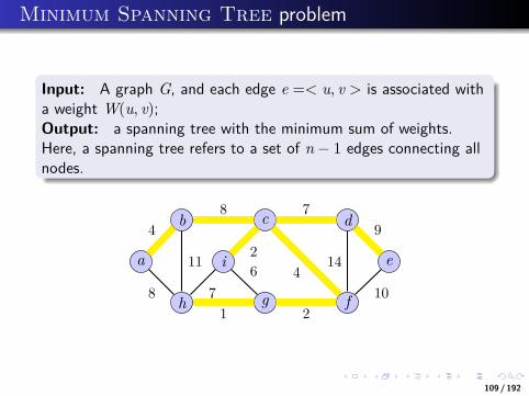
Minimum Spanning Tree problem
Input: A graph G, and each edge e =< u, v > is associated witha weight W(u, v);Output: a spanning tree with the minimum sum of weights.Here, a spanning tree refers to a set of n − 1 edges connecting allnodes.
a
b
h
i
c
g f
d
e
4
8
11
8
2
76
1 2
4
7
14
9
10
109 / 192

...
.
...
.
...
.
...
.
...
.
...
.
...
.
...
.
...
.
...
.
Independent Vector Set versus Acyclic Forest
LinearlyIndependent Set Acyclic Forest
Maximal LinearlyIndependent Set Spanning Tree
Weighted MaximalLinearly
Independent Set
MinimumSpanning Tree
110 / 192

...
.
...
.
...
.
...
.
...
.
...
.
...
.
...
.
...
.
...
.
Generic Spanning Tree algorithm
Objective: to find a spanning tree for graph G;Basic idea: analogue to Maximal Linearly IndependentSet calculation;
GenericSpanningTree(G)
1: F = {};2: while F does not form a spanning tree do3: find an edge (u, v) that is safe for F;4: F = F ∪ {(u, v)};5: end while
Here F denotes an acyclic forest, and F is still acyclic ifadded by a safe edge.
111 / 192

...
.
...
.
...
.
...
.
...
.
...
.
...
.
...
.
...
.
...
.
Examples of safe edge and unsafe edge
a
b
h
i
c
g f
d
e
4
8
11
8
2
76
1 2
4
7
14
9
10
Figure 3: Safe edge
a
b
h
i
c
g f
d
e
4
8
11
8
2
76
1 2
4
7
14
9
10
Figure 4: Unsafe edge112 / 192

...
.
...
.
...
.
...
.
...
.
...
.
...
.
...
.
...
.
...
.
Minimum Spanning Tree algorithms
113 / 192

...
.
...
.
...
.
...
.
...
.
...
.
...
.
...
.
...
.
...
.
Kruskal’s algorithm [1956]
Basic idea: during the execution, F is always an acyclicforest, and the safe edge added to F is always a least-weightedge connecting two distinct components.
Figure 5: Joseph Kruskal
114 / 192

...
.
...
.
...
.
...
.
...
.
...
.
...
.
...
.
...
.
...
.
Kruskal’s algorithm [1956]
MST-Kruskal(G,W)
1: F = {};2: for all vertex v ∈ V do3: MakeSet(v);4: end for5: Sort the edges of E in an nondecreasing order by weight W;6: for each edge (u, v) ∈ E in the order do7: if FindSet(u) = FindSet(v) then8: F = F ∪ {(u, v)};9: Union (u, v);
10: end if11: end forHere, Union-Find structure is used to detect whether a set ofedges form a cycle.(See slides on Union-Find data structure, and a demo of Kruskalalgorithm)
115 / 192
...
.
...
.
...
.
...
.
...
.
...
.
...
.
...
.
...
.
...
.
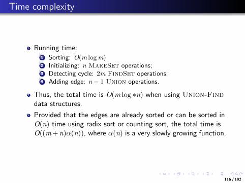
Time complexity
Running time:1 Sorting: O(m logm)2 Initializing: n MakeSet operations;3 Detecting cycle: 2m FindSet operations;4 Adding edge: n − 1 Union operations.
Thus, the total time is O(m log ∗n) when using Union-Finddata structures.Provided that the edges are already sorted or can be sorted inO(n) time using radix sort or counting sort, the total time isO((m+n)α(n)), where α(n) is a very slowly growing function.
116 / 192

...
.
...
.
...
.
...
.
...
.
...
.
...
.
...
.
...
.
...
.
Prim’s algorithm
117 / 192

...
.
...
.
...
.
...
.
...
.
...
.
...
.
...
.
...
.
...
.
Prim’s algorithm [1957]Basic idea: the final minimum spanning tree is grown step bystep. Let’s describe the solving process as a multistagedecision process. At each step, the least-weight edge connectthe sub-tree to a node not in the tree is chosen.Note: One advantage of Prim’s algorithm is that no specialcheck to make sure that a cycle is not formed is required.
Figure 6: Robert C. Prim
118 / 192

...
.
...
.
...
.
...
.
...
.
...
.
...
.
...
.
...
.
...
.
Greedy-selection property
Theorem[Greedy-selection property] Suppose T is a sub-tree of the finalminimum spanning tree, and e = (u, v) is the least-weight edgeconnect one node in T and another node not in T. Then e is inthe final minimum spanning tree.
root
a
b
h g
d
ei
c
f
4
8
11 2
1 2
4
98 7
76 14
10
119 / 192

...
.
...
.
...
.
...
.
...
.
...
.
...
.
...
.
...
.
...
.
Prim algorithm for Minimum Spanning Tree [1957]MST-Prim(G,W, root)1: for all node v ∈ V and v = root do2: key[v] = ∞;3: Π[v] = Null; //Π(v) denotes the predecessor node of v4: PQ.Insert(v); // n times5: end for6: key[root] = 0;7: PQ.Insert(root);8: while PQ = Null do9: u = PQ.ExtractMin(); // n times
10: for all v adjacent with u do11: if W(u, v) < key(v) then12: Π(v) = u;13: PQ.DecreaseKey(W(u, v)); // m times14: end if15: end for16: end whileHere, PQ denotes a min-priority queue. The chain of predecessor nodesoriginating from v runs backwards along a shortest path from s to v.(See a demo) 120 / 192

...
.
...
.
...
.
...
.
...
.
...
.
...
.
...
.
...
.
...
.
Time complexity of Prim algorithm
Operation Linked Binary Binomial Fibonaccilist heap heap heap
MakeHeap 1 1 1 1Insert 1 log n log n 1
ExtractMin n log n log n log nDecreaseKey 1 log n log n 1
Delete n log n log n log nUnion 1 n log n 1
FindMin n 1 log n 1Prim O(n2) O(m log n) O(m log n) O(m + n log n)
Prim algorithm: n Insert, n ExtractMin, and mDecreaseKey.
121 / 192

...
.
...
.
...
.
...
.
...
.
...
.
...
.
...
.
...
.
...
.
Why does the greedy algorithm fail for the weightedIntervalScheduling problem?
122 / 192

...
.
...
.
...
.
...
.
...
.
...
.
...
.
...
.
...
.
...
.
Greedy algorithm fails for the weightedIntervalScheduling problem
Matroid covers many cases of practical interests, and it isuseful when determining whether greedy technique yieldsoptimal solutions. However, greedy algorithm fails for theweighted IntervalScheduling problem.
A1 : w1 = 2
A3 : w3 = 34 A5 : w3 = 3
4
A2 : w2 = 1 A4 : w4 = 0
Solutions: Greedy : {A1,A2,A4} | OPT : {A1,A3,A5}Benefits: 2 + 1 + 0 = 3 | 2 + 3
4 + 34 = 3.5
123 / 192

...
.
...
.
...
.
...
.
...
.
...
.
...
.
...
.
...
.
...
.
Independence in IntervalScheduling problem
A1 : w1 = 2
A3 : w3 = 34 A5 : w3 = 3
4
A2 : w2 = 1 A4 : w4 = 0
Let’s thinks of a set of intervals as “independent” if theydon’t conflict each other. Let N denote the interval set, and Irepresent the family of all independent interval sets.Let’s examine the following properties:
Hereditary property: Any subset of an independent intervalset is still independent.Augmentation property: Consider A = {A1,A3,A5} andB = {A1,A2}. Although |A| > |B|, the augmentation B ∪ {x}with any interval x ∈ A\B is not independent.
Thus M = (N, I) doesn’t form a matroid.We claim that if M = (N, I) doesn’t form a matroid, theredefinitely exists a weighting schema that causes the greedyalgorithm to fail.
124 / 192

...
.
...
.
...
.
...
.
...
.
...
.
...
.
...
.
...
.
...
.
Let’s examine whether the greedy algorithm worksperfectly all the time
TheoremSuppose that M = (N, I) is an independence system, i.e., I hasthe hereditary property. Then M is a matroid iff for anynonnegative weighting schema over N, the greedy algorithmreturns a basis of the maximum weight.
Here each element x ∈ N is associated with a nonnegativeweight w(x), and the weight of a subset S ⊆ N is defined asthe total weights of the elements in S.We consider the greedy algorithm that iteratively adds theheaviest element that maintain independence.
125 / 192

...
.
...
.
...
.
...
.
...
.
...
.
...
.
...
.
...
.
...
.
ProofSuppose we have an independent system M = (N, I) but itdoesn’t satisfy the augmentation property. We prove thetheorem by constructing a weighting schema that causes thegreedy algorithm to fail.Let A, B be independent sets with |A| = |B|+ 1, but theaddition of any element x ∈ A\B to B never gives anindependent set, say A = {A1,A3,A5} and B = {A1,A2} inthe following example.
A1 : w1 = 2
A3 : w3 = 34 A5 : w3 = 3
4
A2 : w2 = 1 A4 : w4 = 0
We construct the following weighting schema:
w(x) =
w1 if x ∈ A ∩ Bw2 if x ∈ B\Aw3 if x ∈ A\Bw4 if x ∈ A ∩ B 126 / 192

...
.
...
.
...
.
...
.
...
.
...
.
...
.
...
.
...
.
...
.
Proof cont’dThe weights w1,w2,w3,w4 were designed as below:
w1 > w2 > w3 > w4 = 0: Thus the greedy algorithm willchoose elements in A ∩ B first, then B\A, and finally A ∩ B.Note that the elements in A\B will not be selected since theaddition of such element to B never gives an independentinterval set.w1|A ∩ B|+ w2|B\A| < w1|A ∩ B|+ w3|A\B|: The first termrepresents the benefits returned by the greedy algorithm, whilethe second one the benefits returned by augmenting based onA. Thus the inequality implies the failure of the greedyalgorithm.
To achieve these two objectives simultaneously, we setw1,w2,w3,w4 as:
w1 = 2w2 = 1
|B\A|
w3 = 1+ϵ|A\B|
w4 = 0
where 0 < ϵ < 1|B\A| . We use ϵ = 1
2 in the above example.127 / 192

...
.
...
.
...
.
...
.
...
.
...
.
...
.
...
.
...
.
...
.
Tight connection between matroid and greedy algorithm
On one side, if you can prove that the problem of interest is amatroid, then you have powerful algorithm automatically.On the other side, if the greedy algorithm works perfectly allthe time, then the problem might be a matroid.
128 / 192

...
.
...
.
...
.
...
.
...
.
...
.
...
.
...
.
...
.
...
.
When greedy strategy is good enough: Maximizing a submodularfunction
129 / 192

...
.
...
.
...
.
...
.
...
.
...
.
...
.
...
.
...
.
...
.
Optimizing a set function
Most combinatorial optimization problems, e.g., MinCut,MaxCut, VertexCover, SetCover, MinimumSpanning Tree, MaxCoverage, aim tomaximize/minimize a set function.These problems have the following form:
max /min f(S)s.t. S ∈ F
Here, S ⊆ N represents a subset of a ground set N, F ⊆ 2N
represents certain constraints over these subsets, and f(S)denotes a set function.
130 / 192

...
.
...
.
...
.
...
.
...
.
...
.
...
.
...
.
...
.
...
.
Let’s start from the MaxCoverage problem
Consider a set of n elements N = {1, 2, ...,n}, and m subsetsA1,A2, ...,Am ⊆ N. The goal of MaxCoverage problem isto select k subsets such that the cardinality of their union ismaximized.
max |∪
Ai∈SAi|
s.t. |S| = k
A1A2
A3
131 / 192

...
.
...
.
...
.
...
.
...
.
...
.
...
.
...
.
...
.
...
.
Set functionThe objective function in the Max Coverage problemf(S) = |
∪Ai∈S
Ai| is a set function defined over subsets.
A1A2
A3
S f(S)ϕ 0
{A3} 16{A2} 12
{A2,A3} 24{A1} 8
{A1,A3} 21{A1,A2} 20
{A1,A2,A3} 28132 / 192

...
.
...
.
...
.
...
.
...
.
...
.
...
.
...
.
...
.
...
.
Set function: another viewpoint from cubeA set function f : {0, 1}m → R defines value for nodes of thecube.
A1A2
A3
f(ϕ) = 0 f({A1}) = 8
f({A2}) = 12
f({A3}) = 16
f({A2, A3}) = 24 f({A1, A2, A3}) = 28
f({A1, A3}) = 21
f({A1, A2}) = 20
S A1 A2 A3 fϕ 0 0 0 0
{A3} 0 0 1 16{A2} 0 1 0 12
{A2,A3} 0 1 1 24{A1} 1 0 0 8
{A1,A3} 1 0 1 21{A1,A2} 1 1 0 20
{A1,A2,A3} 1 1 1 28133 / 192

...
.
...
.
...
.
...
.
...
.
...
.
...
.
...
.
...
.
...
.
Revisiting the continuous optimization
But how to maximize a set function? Let’s revisit thecontinuous maximization first.
y
o x
f(x) y
o x
f(x)
A continuous function f : R → R can be efficiently minimizedif it is convex, and can be efficiently maximized if it isconcave.
134 / 192

...
.
...
.
...
.
...
.
...
.
...
.
...
.
...
.
...
.
...
.
Question: are there discrete analogue to convexity or concavityfor set functions?
135 / 192

...
.
...
.
...
.
...
.
...
.
...
.
...
.
...
.
...
.
...
.
Submodularity: discrete analogue to concavity
Concavity: f(x) is concave if the derivative f′(x) isnon-increasing in x, i.e., when ∆x is sufficiently small,f(x1 +∆x)− f(x1) ≥ f(x2 +∆x)− f(x2) if x1 ≤ x2.
y
o x
f(x)
x1 x2
S1
S2
e
Submodularity: f(S) is submodular if for any element e, themarginal gain (discrete analogy to derivative) f(S + e)− f(S)is non-increasing in S, i.e., if S1 ⊆ S2,f(S1 + e)− f(S1) ≥ f(S2 + e)− f(S2). (For simplicity, we usef(S + e) to represent f(S ∪ {e}) and use f(e) to representf({e}).)
136 / 192

...
.
...
.
...
.
...
.
...
.
...
.
...
.
...
.
...
.
...
.
Submodular functions: decreasing marginal gain
Let’s consider a set function f(S) defined over subsets S ⊆ N,where N is a finite ground set.
Definition (Marginal gain to a subset S )The marginal gain of a subset T to S is defined asfS(T) = f(S ∪ T)− f(S).
Definition (Submodular function f(S) )A set function f : 2N → R is submodular iff ∀S1 ⊆ S2 ⊆ N,∀e ∈ N\S2, fS2(e) ≤ fS1(e). f(S) is supermodular if −f(S) issubmodular, and modular if both sub- and supermodular.
Intuition: marginal gain is discrete analogy to derivative of acontinuous function, while “decreasing marginal gain” (or“diminishing returns”) definition of f(S) is discrete analogy toconcave functions.
137 / 192

...
.
...
.
...
.
...
.
...
.
...
.
...
.
...
.
...
.
...
.
An equivalent definition: subadditive
Definition (Submodular function)A function f : 2N → R is submodular iff ∀A,B ⊆ N,f(A) + f(B) ≥ f(A ∪ B) + f(A ∩ B).
Taking the submodular function f(A) = |∪
i∈ATi| as an
example. Let A = {1, 2}, B = {1, 3}, we havef(A ∪ B) + f(A ∩ B) = |T1 ∪ T2 ∪ T3|+ |T1| (1)
≤ |T1 ∪ T2|+ |T1 ∪ T3| (2)= f(A) + f(B) (3)
T1T2
T3138 / 192

...
.
...
.
...
.
...
.
...
.
...
.
...
.
...
.
...
.
...
.
Equivalence of the two definitions
Subadditivity essentially implies “decreasing marginal gain”,i.e., by setting S1 = A ∩ B, S2 = A, and T = B − A, theinequality f(A ∪ B)− f(A) ≤ f(B)− f(A ∩ B) can be rewrittenas f(S2 ∪ T)− f(S2) ≤ f(S1 ∪ T)− f(S1).
139 / 192

...
.
...
.
...
.
...
.
...
.
...
.
...
.
...
.
...
.
...
.
Examples of submodular functions
140 / 192

...
.
...
.
...
.
...
.
...
.
...
.
...
.
...
.
...
.
...
.
Example 1: Linear function and budget-additive functions
A set function f : 2N → R is linear (also known as additive,modular if f(S) =
∑i∈S wi, where wi denotes weight of
element i ∈ N.Posing an upper-bound limitation on a modular function, wewill have a monotone submodular function,f(S) = min{
∑i∈S wi,B} for any wi > 0, B > 0.
141 / 192

...
.
...
.
...
.
...
.
...
.
...
.
...
.
...
.
...
.
...
.
Example 2: Set systems and coverageGiven a ground set N and several subset A1,A2, ...,An ⊂ N,the coverage function f(S) = |
∪i∈S Ai| is submodular. This
naturally extends to the weighted version: f(S) = w(∪
i∈S Ai),where w : N → R+.
A1A2
A3
f(ϕ) = 0 f({A1}) = 8
f({A2}) = 12
f({A3}) = 16
f({A2, A3}) = 24 f({A1, A2, A3}) = 28
f({A1, A3}) = 21
f({A1, A2}) = 20
S A1 A2 A3 fϕ 0 0 0 0
{A3} 0 0 1 16{A2} 0 1 0 12
{A2,A3} 0 1 1 24{A1} 1 0 0 8
{A1,A3} 1 0 1 21{A1,A2} 1 1 0 20
{A1,A2,A3} 1 1 1 28142 / 192

...
.
...
.
...
.
...
.
...
.
...
.
...
.
...
.
...
.
...
.
Example 3: Cut of graph
Given a graph G =< V,E >. Let f(S) be the number ofedges e = (u, v) such that u ∈ S and v ∈ V − S.
S1S2
u v
f(S) is submodular. For example, in the above figure,f(S1 + u)− f(S1) = 8 − 4 = 4, whilef(S2 + u)− f(S2) = 4 − 6 = −2.
143 / 192

...
.
...
.
...
.
...
.
...
.
...
.
...
.
...
.
...
.
...
.
Example 4: Rank functions of matroid
Given a matroid M = (N, I), the rank functionr(S) = max{|A| : A ⊆ S,A ∈ I} is monotone submodular.This function can also extend to the weighted version, i.e.,r(S) = max{w(A) : A ⊆ S,A ∈ I}, where w : N → R+
represents a non-negative weighting function.For example, r({V1,V2,V3,V4,V5}) = 4.
V1 = [ 1 2 3 4 5 ] W1 = 9V2 = [ 1 4 9 16 25 ] W2 = 7V3 = [ 1 8 27 64 125 ] W3 = 5V4 = [ 1 16 81 256 625 ] W4 = 3V5 = [ 2 6 12 20 30 ] W5 = 1
144 / 192
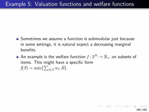
...
.
...
.
...
.
...
.
...
.
...
.
...
.
...
.
...
.
...
.
Example 5: Valuation functions and welfare functions
Sometimes we assume a function is submodular just becausein some settings, it is natural expect a decreasing marginalbenefits.An example is the welfare function f : 2N → R+ on subsets ofitems. This might have a specific formf(S) = min{
∑i∈S wi,B}.
145 / 192

...
.
...
.
...
.
...
.
...
.
...
.
...
.
...
.
...
.
...
.
Example 6: Entropy of joint probability distributution
Given a joint probability distribution P(X) overdiscrete-valued random variables X = [x1, x2, ..., xn], thefunction f(S) = H(XS) is monotone submodular, where H isthe Shannon entropy, i.e.,
H(XS) = −∑i∈S
P(xi) logP(xi)
If the random variables are real-valued, then H(XS) is alsosubmodular but not generally monotone.
146 / 192

...
.
...
.
...
.
...
.
...
.
...
.
...
.
...
.
...
.
...
.
Example 7: Facility location
Given a set of locations N = {1, 2, ...,n} and m customers. Ifwe open up a facility at location j, then it serves customer iwith value Vi,j ≥ 0. Each customer chooses the facility withthe highest value. Thus, suppose we select a set of locationsS ⊆ N to open up facilities, the total value provided for thesecustomers is:
f(S) =m∑
i=1maxj∈S
Vi,j
f(S) is monotone submodular.
147 / 192

...
.
...
.
...
.
...
.
...
.
...
.
...
.
...
.
...
.
...
.
Other examples of submodular functions
Influence of advertisement over social networks: Assume youhave a product and you want to advertise it in a socialnetwork. The problem is how to select nodes in the socialnetwork to maximize the influence.Word alignment: Consider a sentence in Chinese and itstranslation in English. We want to know the correspondenceof words in the two sentences. The correspondence can bedescribed using a bi-partite graph and measured using asubmodular function.Documents summarization: Consider a set of relateddocuments and we want to summarize them. Thesummarization can be measured using a submodular function.
148 / 192

...
.
...
.
...
.
...
.
...
.
...
.
...
.
...
.
...
.
...
.
Properties of submodular functions
149 / 192

...
.
...
.
...
.
...
.
...
.
...
.
...
.
...
.
...
.
...
.
Several properties of submodular functions
1 Non-negative linear combinations of submodular functions arestill submodular, i.e., if f1, f2, ..., fn are submodular on thesame ground set N, and w1,w2, ...,wn are non-negative reals,then w1f1 + w2f2 + ...+ wnfn is also submodular. This isimportant as when we are designing objective functions tomaximize, we can first design some simple submodular pieces,and then combine them.
2 Truncation of monotone submodular functions are stillsubmodular, i.e, min{f(S),C} is submodular when f(S) ismonotone submodular and C is a constant.
3 If f : 2N → R+ is submodular, then the function g defined asg(S) = ϕ(f(S)), where ϕ is concave, is also submodular.
4 f is submodular iff for any S ⊂ N, fS is submodular.
150 / 192
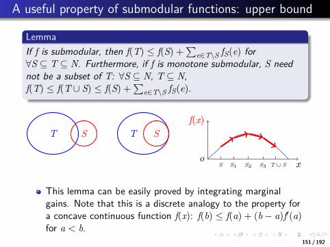
...
.
...
.
...
.
...
.
...
.
...
.
...
.
...
.
...
.
...
.
A useful property of submodular functions: upper bound
LemmaIf f is submodular, then f(T) ≤ f(S) +
∑e∈T\S fS(e) for
∀S ⊆ T ⊆ N. Furthermore, if f is monotone submodular, S neednot be a subset of T: ∀S ⊆ N, T ⊆ N,f(T) ≤ f(T ∪ S) ≤ f(S) +
∑e∈T\S fS(e).
T S T Sf(x)
o xS S1 S2 S3 T ∪ S
This lemma can be easily proved by integrating marginalgains. Note that this is a discrete analogy to the property fora concave continuous function f(x): f(b) ≤ f(a) + (b − a)f′(a)for a < b.
151 / 192

...
.
...
.
...
.
...
.
...
.
...
.
...
.
...
.
...
.
...
.
MaxCoverage problem with cardinality constraint
Now let’s consider the MaxCoverage problem withcardinality constraint first, i.e., select k subsets such thatthe cardinality of their union is maximized, e.g., select 3subsets in the following example.
A1A2
A3
A4
Here we adopt the value query model, i.e., an algorithm canquery a black-box oracle for the value f(S). An algorithmmaking polynomial queries is considered to have polynomialrunning time.We also assume that f is normalized, i.e., f(ϕ) = 0.
152 / 192

...
.
...
.
...
.
...
.
...
.
...
.
...
.
...
.
...
.
...
.
Greedy algorithm (cardinality constraint)
Basic idea: We describe the solving process as a multi-stagedecision process. At each step, we select the item with thelargest marginal gain.
GreedyCardinalityConstraint(k,N)
1: S = ϕ;2: while |S| < k do3: x = argmaxx∈NfS(x);4: S = S ∪ {x};5: N = N − {x};6: end while7: return S;
153 / 192

...
.
...
.
...
.
...
.
...
.
...
.
...
.
...
.
...
.
...
.
An example: Step 1
A1A2
A3
A4
Let Si = {x1, x2, ..., xi} be the value of S after the i-thexecution of the while loop. Initially A3 was selected asfϕ(A3) = 12.
A3
S1 = {A3}f(S)
oSS0 S1
12
154 / 192

...
.
...
.
...
.
...
.
...
.
...
.
...
.
...
.
...
.
...
.
Step 2
A1A2
A3
A4
A1 was selected with fS1(A1) = 10, which is larger thanfS1(A2) = 8, and fS1(A4) = 6.
A1
A3
S2 = {A3,A1}f(S)
oSS0 S1
12
S2
22
155 / 192
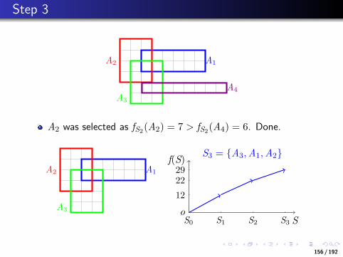
...
.
...
.
...
.
...
.
...
.
...
.
...
.
...
.
...
.
...
.
Step 3
A1A2
A3
A4
A2 was selected as fS2(A2) = 7 > fS2(A4) = 6. Done.
A1A2
A3
S3 = {A3,A1,A2}f(S)
oSS0 S1
12
S2
22
S3
29
156 / 192

...
.
...
.
...
.
...
.
...
.
...
.
...
.
...
.
...
.
...
.
Analysis
TheoremLet Sk = {x1, x2, ..., xk} be the set returned byGreedyCardinalityConstraint, then f(Sk) ≥ (1 − 1
e )f(S∗).
A1A2
A3
S3 = {A3,A1,A2}f(S)
oSS0 S1
12
S2
22
S3
29
Intuition: At each iteration, the gap f(S∗)− f(Si) wasnarrowed down. Let’s consider the boundary case, i.e., afterselecting k elements. In this case, the gap was reduced to beat most 1
k f(S∗).157 / 192

...
.
...
.
...
.
...
.
...
.
...
.
...
.
...
.
...
.
...
.
The gap shrinks exponentially: an example
1 g0 : 302 g1 : 30-12=18, 18 ≤ (1 − 1
3)× 303 g2 : 30-22=8, 8 ≤ (1 − 1
3)× 184 g3 : 30-29=1, 1 ≤ (1 − 1
3)× 8Thus we have g3 ≤ (1 − 1
3)3 × 30 ≤ (1 − 1
e )× 30.
158 / 192

...
.
...
.
...
.
...
.
...
.
...
.
...
.
...
.
...
.
...
.
Proof.Let’s consider the gap gi−1 = f(Si−1)− f(S∗).
f(S∗) ≤ f(Si−1) +∑
e∈S∗\Si−1
fSi−1(e) (4)
≤ f(Si−1) +∑
e∈S∗\Si−1
fSi−1(xi) (5)
= f(Si−1) +∑
e∈S∗\Si−1
(f(Si)− f(Si−1)
)(6)
≤ f(Si−1) + k(f(Si)− f(Si−1)
)(7)
By subtracting kf(S∗) on both sides, we can obtain the inductionrelationship between gi−1 and gi as follows:
f(Si)− f(S∗) ≥ (1 − 1k )(f(Si−1)− f(S∗)
).
By induction we further have f(Si) ≥(1 − (1 − 1
k )i)f(S∗), and thus
after k iterations, f(Sk) ≥(1 − (1 − 1
k )k)f(S∗) ≥ (1 − 1
e )f(S∗).
159 / 192
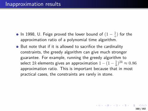
...
.
...
.
...
.
...
.
...
.
...
.
...
.
...
.
...
.
...
.
Inapproximation results
In 1998, U. Feige proved the lower bound of (1 − 1e ) for the
approximation ratio of a polynomial time algorithm.But note that if it is allowed to sacrifice the cardinalityconstraints, the greedy algorithm can give much strongerguarantee. For example, running the greedy algorithm toselect 2k elements gives an approximation 1− (1− 1
k )2k ≈ 0.86
approximation ratio. This is important because that in mostpractical cases, the constraints are rarely in stone.
160 / 192

...
.
...
.
...
.
...
.
...
.
...
.
...
.
...
.
...
.
...
.
MaxCoverage problem under knapsack constraint
161 / 192

...
.
...
.
...
.
...
.
...
.
...
.
...
.
...
.
...
.
...
.
MaxCoverage problem under knapsack constraint
Now let’s further consider the MaxCoverage problemunder knapsack constraint, i.e., each element i ∈ N isassociated with a cost C(Ai), and we have a budget B. Weaim to select subsets such that the total cost is no more thanB and the cardinality of their union is maximized.
max |∪
Ai∈SAi|
s.t.∑
Ai∈S C(Ai) ≤ B
A1 : C(A1) = 46A2 : C(A2) = 41
A3 : C(A3) = 40A4 : C(A4) = 2
B = 88
162 / 192

...
.
...
.
...
.
...
.
...
.
...
.
...
.
...
.
...
.
...
.
Greedy algorithm (knapsack constraint)
Basic idea: We describe the solving process as a multi-stagedecision process. At each step, we select the item with thehighest benefit-cost ratio rather than the item with thelargest marginal gain.
GreedyKnapsackConstraint(N,C,B)
1: S = ϕ;2: while N = NULL do3: x = argmaxx∈N
fS(x)C(x) ;
4: if∑
e∈S C(e) + C(x) ≤ B then5: S = S ∪ {x};6: end if7: N = N − {x};8: end while9: return S;
163 / 192

...
.
...
.
...
.
...
.
...
.
...
.
...
.
...
.
...
.
...
.
An example: Step 1
A1 : C(A1) = 46A2 : C(A2) = 41
A3 : C(A3) = 40A4 : C(A4) = 2
B = 88
Let Si = {x1, x2, ..., xi} be the value of S after the i-thexecution of the while loop. Initially A4 was selected withfϕ(A4)C(A4)
= 82 , which is larger than A1(
1246), A2(
1241) and A3(
1240).
A4
S1 = {A4}f(S)
oSS0 S1
8
164 / 192

...
.
...
.
...
.
...
.
...
.
...
.
...
.
...
.
...
.
...
.
Step 2
A1 : C(A1) = 46A2 : C(A2) = 41
A3 : C(A3) = 40A4 : C(A4) = 2
B = 88
A2 was selected with fS1 (A2)
C(A2)= 12
41 as it is larger thanfS1 (A1)
C(A1)= 12
46 and fS1 (A3)
C(A3)= 10
40 .
A2
A4
S2 = {A4,A2}f(S)
oSS0 S1
8
S2
20
165 / 192
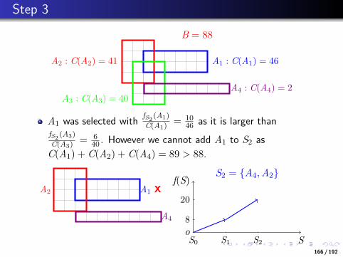
...
.
...
.
...
.
...
.
...
.
...
.
...
.
...
.
...
.
...
.
Step 3
A1 : C(A1) = 46A2 : C(A2) = 41
A3 : C(A3) = 40A4 : C(A4) = 2
B = 88
A1 was selected with fS2 (A1)
C(A1)= 10
46 as it is larger thanfS2 (A3)
C(A3)= 6
40 . However we cannot add A1 to S2 asC(A1) + C(A2) + C(A4) = 89 > 88.
A1 XA2
A4
S2 = {A4,A2}f(S)
oSS0 S1
8
S2
20
166 / 192
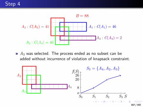
...
.
...
.
...
.
...
.
...
.
...
.
...
.
...
.
...
.
...
.
Step 4
A1 : C(A1) = 46A2 : C(A2) = 41
A3 : C(A3) = 40A4 : C(A4) = 2
B = 88
A3 was selected. The process ended as no subset can beadded without incurrence of violation of knapsack constraint.
A2
A3
A4
S3 = {A4,A2,A3}f(S)
oSS0 S1
8
S2
20
S3
26
167 / 192

...
.
...
.
...
.
...
.
...
.
...
.
...
.
...
.
...
.
...
.
AnalysisUnfortunately, the GreedyKanpsackConstraintalgorithm has an unbounded approximation ratio.Consider the following instance: N = {e1, e2}, and C(e1) = 1,C(e2) =
ϵ2 (1 > ϵ > 0), and B = 1. The set function is
f({e1}) = 1, and f({e2}) = ϵ.
A1
f({A1}) = 1C(A1) = 1
A2
f({A2}) = ϵC(A2) =
ϵ2
B = 1
The optimal solution is S∗ = {e1} with f(S∗) = 1. In contrast,the GreedyKanpsackConstraint algorithm returnsS∗ = {e2} with f(S∗) = ϵ. As ϵ approaches to 0, theapproximation ratio becomes arbitrarily large.Reason: the algorithm selects elements according tobenefit-cost ratio but totally ignores the value of elements.
168 / 192

...
.
...
.
...
.
...
.
...
.
...
.
...
.
...
.
...
.
...
.
Let consider the boundary case of knapsack constraint
TheoremLet Si be the value of S at the i-th iteration. Suppose the additionof x to Si incurs the violation of the knapsack constraint, i.e.,C(Si) + C(x) > B, then f(Si + x) ≥ (1 − 1
e )f(S∗).
...
... ... ...
... ... ...... ......
... ......
x1
x2
x3
x∗1
x∗2
x∗3 x′
S∗1
S∗2
S∗
Si
Si + x′
Intuition: at each iteration, the gap f(S∗)− f(Si) wasnarrowed down. The occurrence of the violation of knapsackconstraint implies that the algorithm reaches a “boundary”. Inthis case, if adding one more element is permitted, we willobtain an upper bound for f(S∗).
169 / 192

...
.
...
.
...
.
...
.
...
.
...
.
...
.
...
.
...
.
...
.
An example
X A1 : C(A1) = 46A2 : C(A2) = 41
A4 : C(A4) = 2
B = 88 S2 = {A4,A2}
In the above example, A1 was selected as it has the highestbenefit-cost ratio fS2 ({A1})
C(A1)= 10
46 . We cannot add A1 toS2 = {A4,A2} as C(S2) + C(A1) = 89 > 88; however, theaddition of A1 provides an upper bound for f(S∗), i.e.,f({A4,A2,A1}) = 30 ≥ (1 − 1
e )f(S∗).
170 / 192

...
.
...
.
...
.
...
.
...
.
...
.
...
.
...
.
...
.
...
.
Proof
Let’s denote Si = {x1, x2, ..., xi} and examine the gapf(Si−1)− f(S∗).
f(S∗) ≤ f(Si−1) +∑
x∈S∗\Si−1fSi−1(x) (8)
= f(Si−1) +∑
x∈S∗\Si−1fSi−1(x)
C(x)C(x) (9)
≤ f(Si−1) +∑
x∈S∗\S−1C(x)
fSi−1(xi)
C(xi)(10)
≤ f(Si−1) + BfSi−1(xi)
C(xi)(11)
= f(Si−1) + Bf(Si)− f(Si−1)
C(xi)(12)
Next we can obtain the following recursion of gaps:f(Si)− f(S∗) ≥ (1 − C(xi)
B )(f(Si−1)− f(S∗)
).
171 / 192

...
.
...
.
...
.
...
.
...
.
...
.
...
.
...
.
...
.
...
.
Proof (continued)
Solving the recursion, we obtain the following bound:
f(Si) ≥ (1 −i∏
k=1
(1 − C(xk)
B ))f(S∗) (13)
≥ (1 − e−C(Si)
B )f(S∗) (14)
Now consider the boundary case of the increase in f(Si), i.e.,C(Si) + C(x) > B, then if adding one more element waspermitted:
f(Si ∪ {x}) ≥ (1 − e−C(Si)+C(x)
B )f(S∗) (15)
≥ (1 − t1e )f(S
∗) (16)
172 / 192

...
.
...
.
...
.
...
.
...
.
...
.
...
.
...
.
...
.
...
.
Improvement of GreedyKanpsackConstraint:considering the value of elements [Leskovec, 2007]
Basic idea: By considering the value of elements, thealgorithm partly circumvents the shortcoming ofGreedyKnapsackConstraint. In the above example, thealgorithm returns {A1} rather than {A2}.
GreedyKnapsackConstraint2(N,C,B)
1: e∗ = argmaxe∈N,C(e)≤Bf({e});2: SG1 =GreedyKnapsackConstraint(N,C,B);3: return max{f(SG1), f({e∗})};
A1
f({A1}) = 1C(A1) = 1
A2
f({A2}) = ϵC(A2) =
ϵ2
B = 1
173 / 192

...
.
...
.
...
.
...
.
...
.
...
.
...
.
...
.
...
.
...
.
Analysis
Theoremf(SG2) ≥ 1
2(1 − 1e )f(S
∗), where SG2 denotes the set returned byGreedyKnapsackConstraint2.
Proof.After the last element of SG1 was added, the while loop inGreedyKnapsackConstraint1 should be executed atleast once (an auxiliary element can be added to guaranteethis).At these iterations, line 5 was evaluated to FALSE, i.e.,C(SG1) + C(x) > B. We consider the first iteration:
2f(SG2) ≥ f(SG1) + f(e∗) (17)≥ f(SG1) + f(x) (18)≥ f(SG1 + x) (19)≥ (1 − 1
e )f(S∗) (20)
174 / 192

...
.
...
.
...
.
...
.
...
.
...
.
...
.
...
.
...
.
...
.
Improvement of GreedyKnapsackConstraint:Starting from a good initial set
S∗d S∗SG
Basic idea: The algorithm circumvents the shortcoming ofGreedyKnapsackConstraint by considering value ofitems. Specifically, we divide S∗ into two parts, namely, S∗
dand S∗ − S∗
d, where S∗d contains the top d items with large
contribution to f(S∗). Thus, if we run greedy algorithmstarting from the good initial set S∗
d, the marginal gain ofany element will not be higher than the average of f(S∗
d).Question: How to obtain a good initial set?
175 / 192
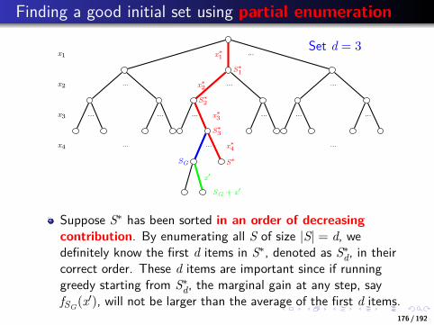
...
.
...
.
...
.
...
.
...
.
...
.
...
.
...
.
...
.
...
.
Finding a good initial set using partial enumeration
...
... ... ...
... ... ...... ......
... ......
x1
x2
x3
x4
x∗1
x∗2
x∗3
x∗4
x′
S∗1
S∗2
S∗3
S∗SG
SG + x′
Set d = 3
Suppose S∗ has been sorted in an order of decreasingcontribution. By enumerating all S of size |S| = d, wedefinitely know the first d items in S∗, denoted as S∗
d, in theircorrect order. These d items are important since if runninggreedy starting from S∗
d, the marginal gain at any step, sayfSG(x′), will not be larger than the average of the first d items.
176 / 192

...
.
...
.
...
.
...
.
...
.
...
.
...
.
...
.
...
.
...
.
Greedy with partial enumeration [Khuller 1999, Sviridenko2004]
GreedyKnapsackConstraint3(N,C,B)
1: S′ = argmaxC(S)≤B,|S|<df(S);2: for all S such that C(S) ≤ B, |S| = d do3: N′ = N − S;4: SG1 = Running GreedyKnapsackConstraint on N′ with S
as initial set;5: if f(SG1) > f(S′) then6: S′ = SG1 ;7: end if8: end for9: return S′;
177 / 192

...
.
...
.
...
.
...
.
...
.
...
.
...
.
...
.
...
.
...
.
Analysis
TheoremLet S∗ denote the optimal solution, and SG denote the setreturned by GreedyKnapsackConstraint3. By setting d = 3,f(SG) ≥ (1 − 1
e )f(S∗).
S∗d S∗SG
178 / 192

...
.
...
.
...
.
...
.
...
.
...
.
...
.
...
.
...
.
...
.
Proof.Let’s write S∗ as S∗ = {x∗1, x∗2, ..., x∗k}, and denote the first iitems as S∗
i = {x∗1, x∗2, ..., x∗i }. Here these items are sorted in adecreasing order of marginal gain, i.e.,x∗i = argmaxx∈S∗\Si−1fS∗
i−1(x).
First, we claim that after d iterations, the marginal gain ofany element is upper-bounded. In particular, 1
d f(S∗d) ≥ fSG(x′),
where S∗d ⊆ SG, and adding x′ to SG leads to the violation of
knapsack constraint.Second, running GreedyKnapsackConstraint usingS = S∗
d as initial set is equivalent to running with initial setS = ϕ, N′ = N\S∗
d, and set function fS∗d. As fS∗
dis also
sub-modular, f(SG + x′)− f(S∗d) ≥
(1 − 1
e )(f(S∗)− f(S∗
d)).
f(SG) = f(SG + x′)− fSG(x′) (21)
≥ f(SG + x′)− 1d f(S∗
d) (22)≥ (1 − 1
e )f(S∗) + (1
e − 1d)f(S
∗d) (23)
≥ (1 − 1e )f(S
∗) (24)179 / 192

...
.
...
.
...
.
...
.
...
.
...
.
...
.
...
.
...
.
...
.
S∗d provides upper bound for marginal gain in further steps
LemmaAfter d iterations, the marginal gain of any element isupper-bounded. In particular, 1
d f(S∗d) ≥ fSG(x′), where S∗
d ⊆ SG,and adding x′ to SG leads to the violation of knapsack constraint.
Proof.Note that the items in S∗ are sorted in a decreasing order ofmarginal gain, i.e., x∗i = argmaxx∈S∗\Si−1fS∗
i−1(x).
Thus for 1 ≤ k ≤ d,
fSG(x′) ≤ fS∗
k−1(x′) (25)
≤ f(S∗k−1 + x∗k)− f(S∗
k−1) (26)≤ f(S∗
k)− f(S∗k−1) (27)
Summing for 1 ≤ k ≤ d, we have: fSG(x′) ≤ 1d f(S∗
d).
180 / 192

...
.
...
.
...
.
...
.
...
.
...
.
...
.
...
.
...
.
...
.
MaxCoverage problem under matroid constraint
181 / 192

...
.
...
.
...
.
...
.
...
.
...
.
...
.
...
.
...
.
...
.
MaxCoverage problem under matroid constraint
Now let’s further consider the MaxCoverage problem withmatroid constraint, i.e., given a matroid M = (N, I), whereI represents independent subsets of N.We aim to select an independent subset S from I such thatf(S) is maximized.
max f(S)s.t. S ∈ I
182 / 192

...
.
...
.
...
.
...
.
...
.
...
.
...
.
...
.
...
.
...
.
An example: Welfare maximization
Welfare maximization problem: Consider m itemsI = {I1, I2, ..., Im} and n people. Each people i is associatedwith a submodular valuation function fi : 2M → R+. Theobjective is to partition M into M = S1 ∪ S2 ∪ ... ∪ Sn suchthat the total valuation
∑ni=1 fi(Si) is maximized.
Construct a partition matroid: We first create n clones of eachitems, denoted as N = {I11, I12, ..., Imn}, where item Iij hasthe color j. Then we think of a set of items as independent ifno pair of items have identical color. Thus we construct apartition matroid M = (N, I), where I = {S : |S ∩ Ii| ≤ 1}.Thus, the welfare maximization problem is equivalent tomax f(S)s.t.S ∈ I.
183 / 192

...
.
...
.
...
.
...
.
...
.
...
.
...
.
...
.
...
.
...
.
GreedyMatroidConstraint algorithm [Nemhauser,1978]
Basic idea: at each iteration, the element x′ with the largestmarginal gain was added to S if S ∪ {x′} is independent. Notethat the set returned is a base of M.
GreedyMatroidConstraint(N, I)1: S = ϕ;2: while N = {} do3: x′ = argmaxx∈NfS(x);4: if S ∪ {x′} ∈ I then5: S = S ∪ {x′};6: end if7: N = N − x′;8: end while9: return S;
184 / 192

...
.
...
.
...
.
...
.
...
.
...
.
...
.
...
.
...
.
...
.
Analysis
TheoremLet S be the set returned by GreedyMatroidConstraint,then f(S) ≥ 1
2 f(S∗).
Let’s write S∗ = {x∗1, ..., x∗r}, where r denotes the rank of M.We order S as S = {x′1, ..., x′r}, where x′i = ϕ(x∗i ), and ϕ()represents the bijective basis exchange function between S∗
and S. Then,f(S∗) ≤ f(S) +
∑x∗i ∈S∗\S
fS(x∗i ) (28)
≤ f(S) +∑
x∗i ∈S∗fS(x∗i ) (29)
≤ f(S) +∑r
i=1fSi−1(x∗i ) (30)
≤ f(S) +∑r
i=1fSi−1(x′i) (31)
≤ f(S) +∑r
i=1(f(Si)− f(Si−1)) (32)
≤ 2f(S) (33)185 / 192

...
.
...
.
...
.
...
.
...
.
...
.
...
.
...
.
...
.
...
.
Speeding up greedy algorithm through avoiding redundantevaluations of f(S)
186 / 192

...
.
...
.
...
.
...
.
...
.
...
.
...
.
...
.
...
.
...
.
Reducing the number of evaluationsMotivation: In some applications, the evaluation of the setfunction f(S) might be expensive. For example, evaluating theinfluence of advertisement in social networks requirescomputationally expensive simulations.The standard greedy algorithm commonly requires a largenumber of evaluations of f(S) due to the argmax operationat each iteration. For example, there are O(kn) evaluationsin GreedyCardinalityConstraint algorithm.GreedyCardinalityConstraint(k,N)
1: S = ϕ;2: while |S| < k do3: x = argmaxx∈NfS(x);4: S = S ∪ {x};5: N = N − {x};6: end while7: return S;
Question: could we identify redundant evaluations and thusreduce the number of the evaluation of f(S)?
187 / 192
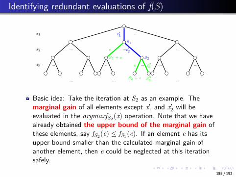
...
.
...
.
...
.
...
.
...
.
...
.
...
.
...
.
...
.
...
.
Identifying redundant evaluations of f(S)
...
... ... ...
... ... ...... ......
... ......
x1
x2
x3
x′1
x′2e
x′′3e
S1
S2S1 + e
S2 + e S′′3
Basic idea: Take the iteration at S2 as an example. Themarginal gain of all elements except x′1 and x′2 will beevaluated in the argmaxfS2(x) operation. Note that we havealready obtained the upper bound of the marginal gain ofthese elements, say fS2(e) ≤ fS1(e). If an element e has itsupper bound smaller than the calculated marginal gain ofanother element, then e could be neglected at this iterationsafely.
188 / 192

...
.
...
.
...
.
...
.
...
.
...
.
...
.
...
.
...
.
...
.
AcceleratedGreedy algorithm [Minoux, 1978]
AcceleratedGreedy(k,N)
1: S = ϕ;2: Set U(x) = f(x) for all x ∈ N;3: while |S| < k do4: while TRUE do5: x = argmaxx∈NU(x);6: if x has already been selected once then7: break;8: end if9: Calculate fS(x) and update U(x) = fS(x);
10: if fS(x) > maxx∈N,x=x U(x) then11: break;12: end if13: end while14: S = S ∪ {x};15: N = N − {x};16: end while17: return S;
189 / 192

...
.
...
.
...
.
...
.
...
.
...
.
...
.
...
.
...
.
...
.
Performance analysis by M. Minoux
When function f is submodular, the accelerated greedyalgorithm produces a greedy solution; furthermore, it producesidentical solution to the corresponding standard greedyalgorithm if the greedy solution is unique.When applied to the optimal network problem, the acceleratedgreedy algorithm requires on average only 2-3 calculations of fat each iteration, leading to a significant speed-up of nearly n
6 .For example, on graphs with about 180 nodes and 500 edges,the accelerated greedy algorithm is 50-100 times faster thanthe standard greedy algorithm.
190 / 192

...
.
...
.
...
.
...
.
...
.
...
.
...
.
...
.
...
.
...
.
A tightly-related problem: MinCost Coverage
191 / 192

...
.
...
.
...
.
...
.
...
.
...
.
...
.
...
.
...
.
...
.
MinCost Coverage problem
In contrast to maximizing a monotone submodular functionunder cardinality constraint, the MinCost Coverageproblem aims to find the minimum sets that achieves a givenamount of objective function value.
min |S|s.t. f(S) ≥ C
For example, the SetCover probem aims to find theminimum number of sets that covers the ground set.
192 / 192

...
.
...
.
...
.
...
.
...
.
...
.
...
.
...
.
...
.
...
.
Greedy algorithm for MinCost Coverage [Wolsey,1982]
TheoremConsider a monotone, submodular, and integer-valued set functionf : 2N → N. Let S0,S1, ... be the sets returned by theGreedyCardinalityConstraint algorithm, and let l be thesmallest index such that f(Sl) ≥ C. Thenl ≤ (1 + lnmaxx∈N f(x))OPTwhere OPT denotes the optimum.
193 / 192