CS 4705

Lecture 14

Corpus Linguistics II

Relating Conditionals and Priors

• P(A | B) = P(A ^ B) / P(B) – Or, P(A ^ B) = P(A | B) P(B)

• Bayes Theorem lets us calculate P(B|A) in terms of P(A|B), e.g. P(to|want) via P(want|to)– P(B|A) = P(B ^ A)/P(A) = P(A|B)P(B)/P(A)

– I.e. calculate probability of next word in sequence from unigram and bigram probabilities we’ve seen

– P(to|want) = P(to ^ want)/P(want) = P(want|to)P(to)/P(want)

Example

F F F F F F I I I I

• P(Finn) = .6

• P(skier) = .5

• P(skier ^ Finn) = .4

• P(skier|Finn) = .67

• P(Finn|skier) = .8

• P(skier|Finn) = P(skier ^ Finn)/P(Finn) = .4/.6 = .67

• P(Finn|skier) = P(Finn ^ skier)/P(skier) = .4/.5 = .8

• P(Finn|skier) = P(skier|Finn) P(Finn)/P(skier) = (.67 * .6)/.5 = .8

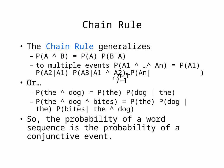
Chain Rule

• The Chain Rule generalizes – P(A ^ B) = P(A) P(B|A)– to multiple events P(A1 ^ …^ An) = P(A1) P(A2|A1)

P(A3|A1 ^ A2)…P(An| )

• Or… – P(the ^ dog) = P(the) P(dog | the)– P(the ^ dog ^ bites) = P(the) P(dog | the) P(bites| the ^

dog)

• So, the probability of a word sequence is the probability of a conjunctive event.

11

ni

• Relative word frequencies are better than equal probabilities for all words– In a corpus with 10K word types, each word would

have P(w) = 1/10K

– Does not match our intuitions that different words are more likely to occur (e.g. the)

• Conditional probability more useful than individual relative word frequencies – Dog may be relatively rare in a corpus

– But if we see barking, P(dog|barking) may be very large

For a Word String

• In general, the probability of a complete string of words w1…wn is

P(w1..n) = P(w1)P(w2|w1)P(w3|w1..w2)…P(wn|w1…wn-1) =

• But this approach to determining the probability of a word sequence is not very helpful in general….

)11|

1( wk

n

kwkP

Markov Assumption

• P(wN) can be approximated using only N-1 previous words of context– This lets us collect statistics in practice

– A bigram model: P(the barking dog) = P(the|<start>)P(barking|the)P(dog|barking)

• Markov models are the class of probabilistic models that assume that we can predict the probability of some future unit without looking too far into the past

• Order of a Markov model: length of prior context

Counting Words in Corpora

• Probabilities are based on counting things, so ….• What should we count?• Words, word classes, word senses, speech acts …?• What is a word?

– e.g., are cat and cats the same word?

– September and Sept?

– zero and oh?

– Is seventy-two one word or two? AT&T?

• Where do we find the things to count?

Corpora

• Corpora are (generally online) collections of text and speech

• e.g.– Brown Corpus (1M words)

– Wall Street Journal and AP News corpora

– ATIS, Broadcast News (speech)

– TDT (text and speech)

– Switchboard, Call Home (speech)

– TRAINS, FM Radio (speech)

Training and Testing

• Probabilities come from a training corpus, which is used to design the model.– overly narrow corpus: probabilities don't generalize

– overly general corpus: probabilities don't reflect task or domain

• A separate test corpus is used to evaluate the model, typically using standard metrics– held out test set

– cross validation

– evaluation differences should be statistically significant

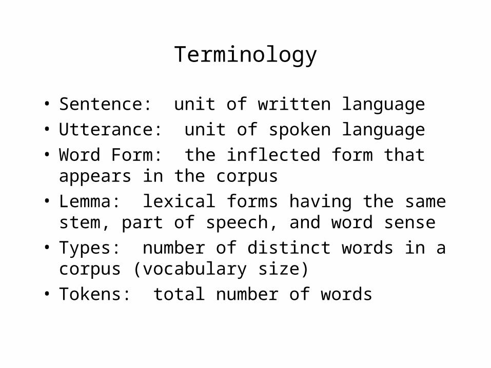
Terminology

• Sentence: unit of written language• Utterance: unit of spoken language• Word Form: the inflected form that appears in the

corpus• Lemma: lexical forms having the same stem, part

of speech, and word sense• Types: number of distinct words in a corpus

(vocabulary size)• Tokens: total number of words

Simple N-Grams

• An N-gram model uses the previous N-1 words to predict the next one:– P(wn | wn -1)

– We'll pretty much always be dealing with P(<word> | <some prefix>)

• unigrams: P(dog)• bigrams: P(dog | big)• trigrams: P(dog | the big)• quadrigrams: P(dog | chasing the big)

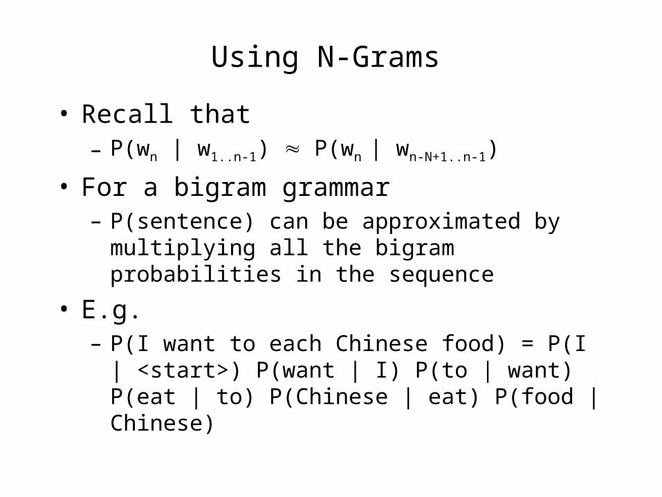
Using N-Grams

• Recall that– P(wn | w1..n-1) P(wn | wn-N+1..n-1)

• For a bigram grammar– P(sentence) can be approximated by multiplying all the

bigram probabilities in the sequence

• E.g. – P(I want to each Chinese food) = P(I | <start>) P(want |

I) P(to | want) P(eat | to) P(Chinese | eat) P(food | Chinese)

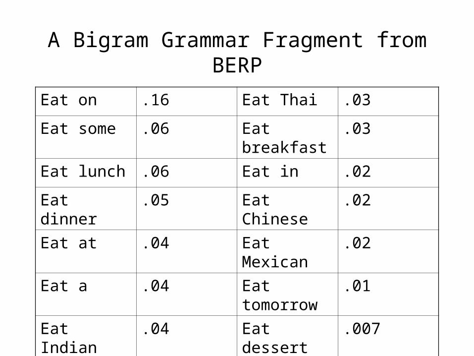
A Bigram Grammar Fragment from BERP

Eat on .16 Eat Thai .03

Eat some .06 Eat breakfast .03

Eat lunch .06 Eat in .02

Eat dinner .05 Eat Chinese .02

Eat at .04 Eat Mexican .02

Eat a .04 Eat tomorrow .01

Eat Indian .04 Eat dessert .007

Eat today .03 Eat British .001

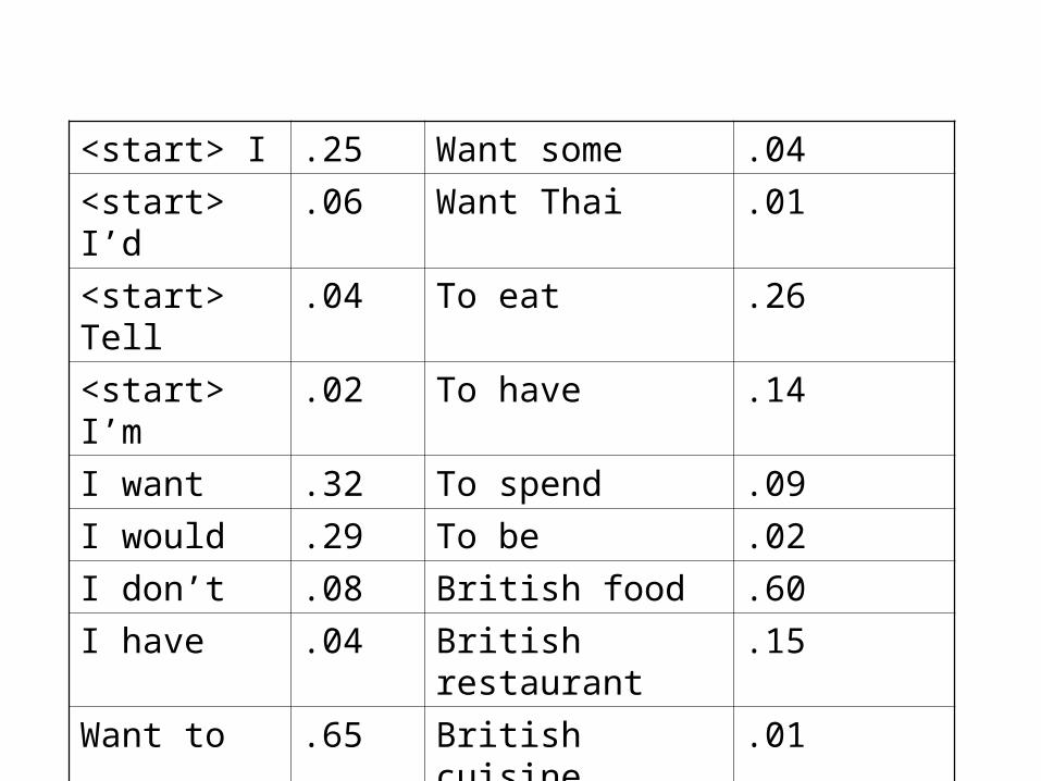
<start> I .25 Want some .04

<start> I’d .06 Want Thai .01

<start> Tell .04 To eat .26

<start> I’m .02 To have .14

I want .32 To spend .09

I would .29 To be .02

I don’t .08 British food .60

I have .04 British restaurant .15

Want to .65 British cuisine .01

Want a .05 British lunch .01

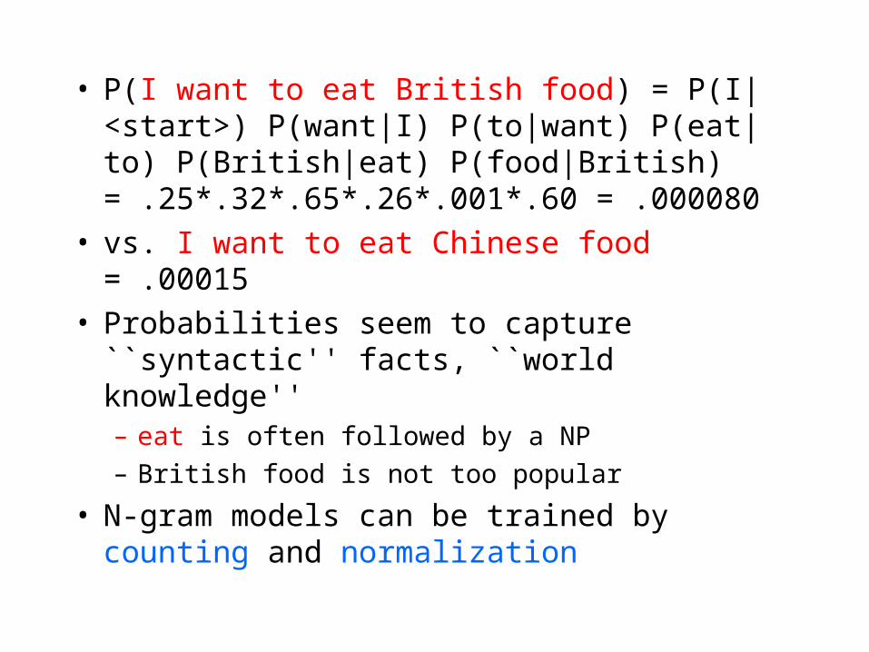
• P(I want to eat British food) = P(I|<start>) P(want|I) P(to|want) P(eat|to) P(British|eat) P(food|British) = .25*.32*.65*.26*.001*.60 = .000080

• vs. I want to eat Chinese food = .00015• Probabilities seem to capture ``syntactic'' facts,

``world knowledge'' – eat is often followed by a NP

– British food is not too popular

• N-gram models can be trained by counting and normalization

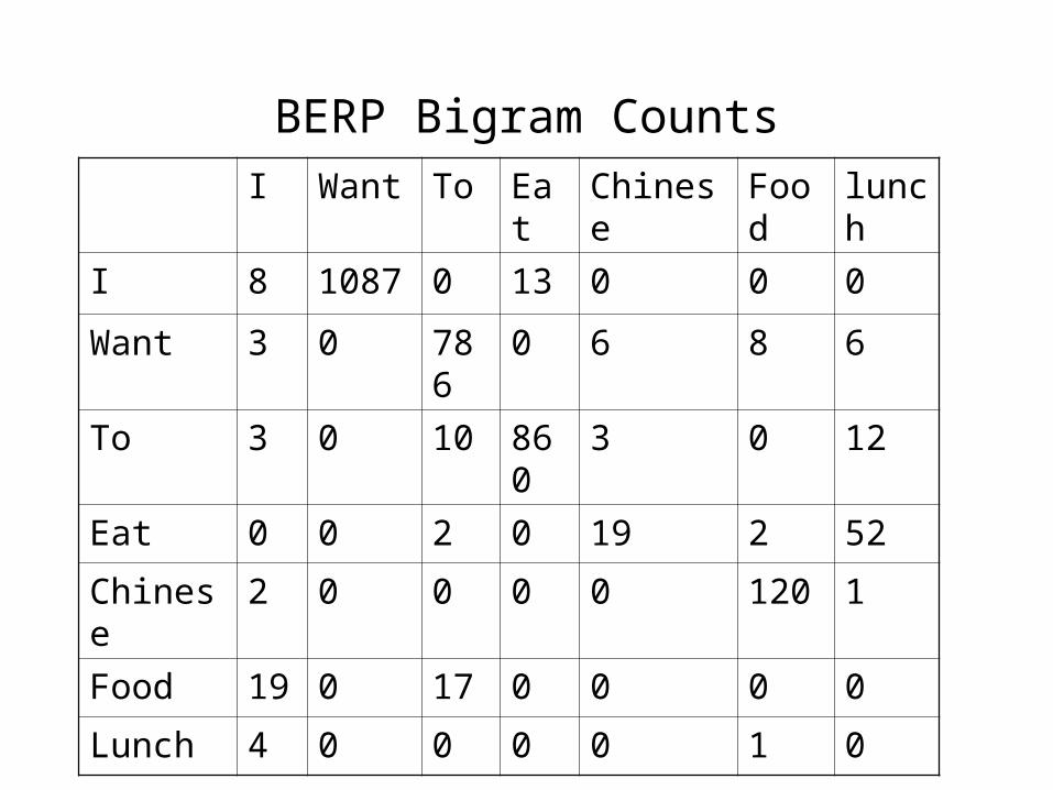
BERP Bigram Counts

I Want To Eat Chinese Food lunch

I 8 1087 0 13 0 0 0

Want 3 0 786 0 6 8 6

To 3 0 10 860 3 0 12

Eat 0 0 2 0 19 2 52

Chinese 2 0 0 0 0 120 1

Food 19 0 17 0 0 0 0

Lunch 4 0 0 0 0 1 0

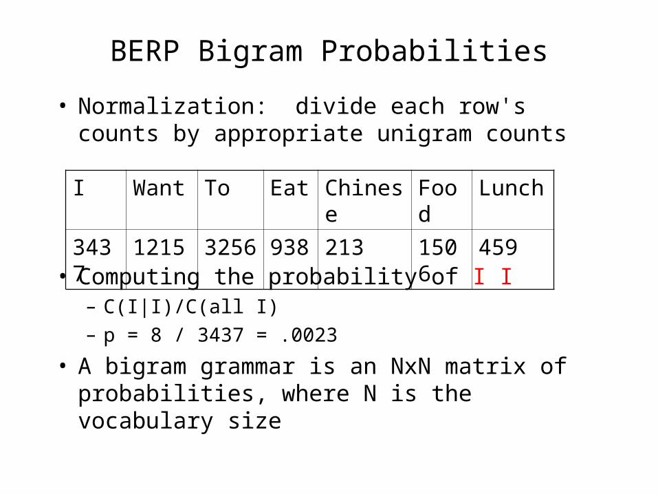
BERP Bigram Probabilities

• Normalization: divide each row's counts by appropriate unigram counts

• Computing the probability of I I– C(I|I)/C(all I)

– p = 8 / 3437 = .0023

• A bigram grammar is an NxN matrix of probabilities, where N is the vocabulary size

I Want To Eat Chinese Food Lunch

3437 1215 3256 938 213 1506 459

What do we learn about the language?

• What's being captured with ...– P(want | I) = .32

– P(to | want) = .65

– P(eat | to) = .26

– P(food | Chinese) = .56

– P(lunch | eat) = .055

• What about...– P(I | I) = .0023

– P(I | want) = .0025

– P(I | food) = .013

– P(I | I) = .0023 I I I I want

– P(I | want) = .0025 I want I want

– P(I | food) = .013 the kind of food I want is ...

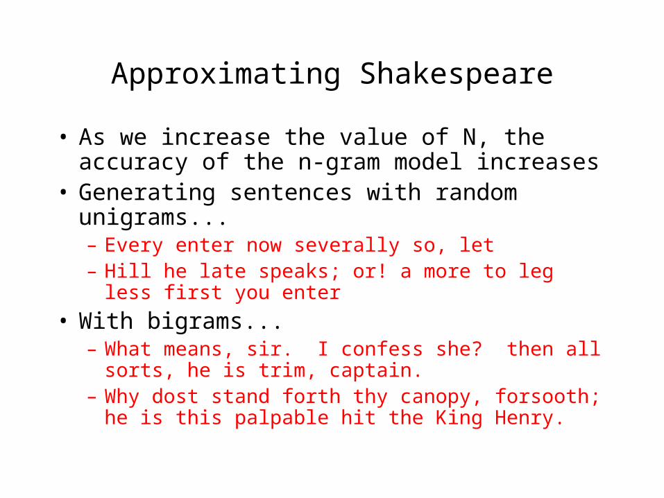
Approximating Shakespeare

• As we increase the value of N, the accuracy of the n-gram model increases

• Generating sentences with random unigrams...– Every enter now severally so, let– Hill he late speaks; or! a more to leg less first you enter

• With bigrams...– What means, sir. I confess she? then all sorts, he is

trim, captain.– Why dost stand forth thy canopy, forsooth; he is this

palpable hit the King Henry.

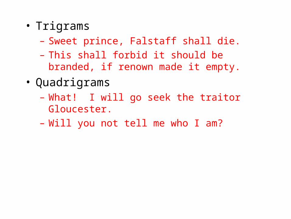
• Trigrams– Sweet prince, Falstaff shall die.

– This shall forbid it should be branded, if renown made it empty.

• Quadrigrams– What! I will go seek the traitor Gloucester.

– Will you not tell me who I am?

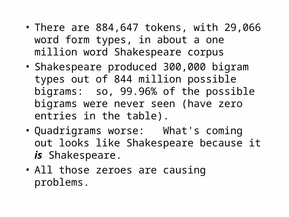
• There are 884,647 tokens, with 29,066 word form types, in about a one million word Shakespeare corpus

• Shakespeare produced 300,000 bigram types out of 844 million possible bigrams: so, 99.96% of the possible bigrams were never seen (have zero entries in the table).

• Quadrigrams worse: What's coming out looks like Shakespeare because it is Shakespeare.

• All those zeroes are causing problems.

N-Gram Training Sensitivity

• If we repeated the Shakespeare experiment but trained on a Wall Street Journal corpus, there would be little overlap in the output

• This has major implications for corpus selection or design

Some Useful Empirical Observations

• A small number of events occur with high frequency

• A large number of events occur with low frequency

• You can quickly collect statistics on the high frequency events

• You might have to wait an arbitrarily long time to get valid statistics on low frequency events

• Some of the zeroes in the table are really zeroes. But others are simply low frequency events you haven't seen yet. How to fix?

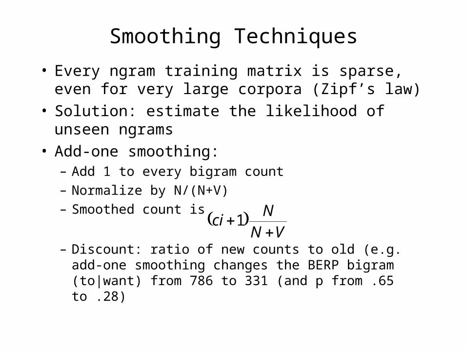
Smoothing Techniques

• Every ngram training matrix is sparse, even for very large corpora (Zipf’s law)

• Solution: estimate the likelihood of unseen ngrams• Add-one smoothing:

– Add 1 to every bigram count

– Normalize by N/(N+V)

– Smoothed count is

– Discount: ratio of new counts to old (e.g. add-one smoothing changes the BERP bigram (to|want) from 786 to 331 (and p from .65 to .28)

VN

Nci

1

• We’d like to find methods that don’t change the original probabilities so drastically

• Witten-Bell Discounting– A zero ngram is just an ngram you haven’t seen yet…– Model unseen bigrams by the ngrams you’ve only seen

once (i.e. the total number of word types in the corpus)– Total probability of unseen bigrams estimated as

– View training corpus as series of events, one for each token (N) and one for each new type (T)

– We can divide the probability mass equally among unseen bigrams….or we can condition the probability of an unseen bigram on the first word of the bigram

TNT

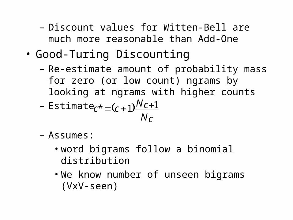
– Discount values for Witten-Bell are much more reasonable than Add-One

• Good-Turing Discounting– Re-estimate amount of probability mass for zero (or

low count) ngrams by looking at ngrams with higher counts

– Estimate

– Assumes:

• word bigrams follow a binomial distribution

• We know number of unseen bigrams (VxV-seen)

Nc

Nccc 11*

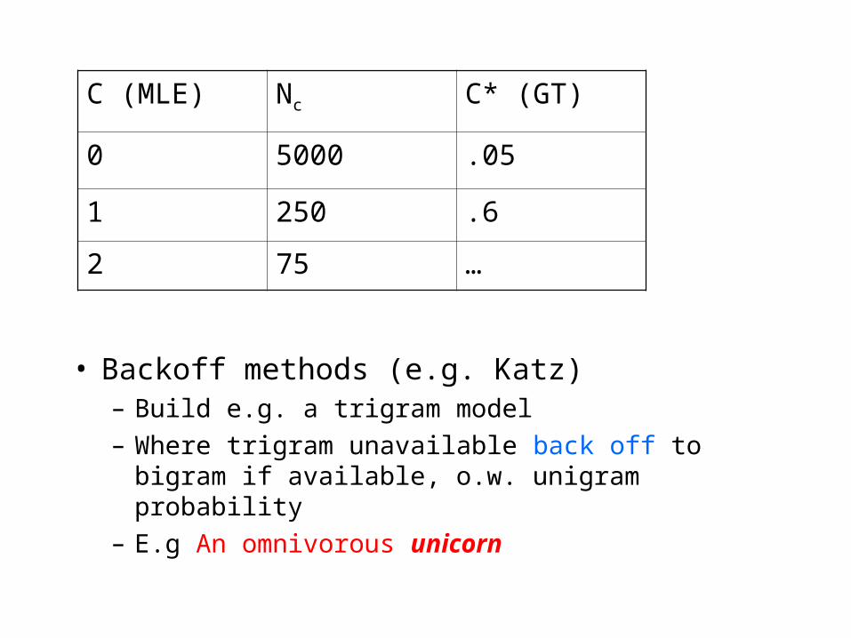
• Backoff methods (e.g. Katz)– Build e.g. a trigram model

– Where trigram unavailable back off to bigram if available, o.w. unigram probability

– E.g An omnivorous unicorn

C (MLE) Nc C* (GT)

0 5000 .05

1 250 .6

2 75 …

Next class

• Midterm• Next class:

– Hindle & Rooth 1993

– Begin studying semantics, Ch. 14