Embed Size (px)
Citation preview

CS 296.4
Mathematical Modelling of Continuous Systems
Carlo TomasiDuke University
Fall 2002

2

Chapter 1
Introduction
Robotics and computer vision are interdisciplinary subjects at the intersection of engineering and computerscience. By their nature, they deal with both computers and the physical world. Although the former arein the latter, the workings of computers are best described in the black-and-white vocabulary of discretemathematics, which is foreign to most classical models of reality, quantum physics notwithstanding.
This class surveys some of the key tools of applied math to be used at the interface of continuous anddiscrete. It is not on robotics or computer vision. These subjects evolve rapidly, but their mathematicalfoundations remain. Even if you will not pursue either field, the mathematics that you learn in this class willnot go wasted. To be sure, applied mathematics is a discipline in itself and, in many universities, a separatedepartment. Consequently, this class can be a quick tour at best. It does not replace calculus or linearalgebra, which are assumed as prerequisites, nor is it a comprehensive survey of applied mathematics. Whatis covered is a compromise between the time available and what is useful and fun to talk about. Even if insome cases you may have to wait until you take a robotics or vision class to fully appreciate the usefulnessof a particular topic, I hope that you will enjoy studying these subjects in their own right.
1.1 Who Should Take This Class
The main goal of this class is to present a collection of mathematical tools for both understanding and solvingproblems in robotics and computer vision. Several classes at most universities cover the topics presented inthis class, and do so in much greater detail. If you want to understand the full details of any one of the topicsin the syllabus below, you should take one or more of these other classes instead. If you want to understandhow these tools are implemented numerically, you should take one of the classes in the scientific computingprogram, which again cover these issues in much better detail. Finally, if you want to understand roboticsor vision, you should take classes in these subjects, since this course is not on robotics or vision.
On the other hand, if you do plan to study robotics, vision, or other similar subjects in the future, andyou regard yourself as a user of the mathematical techniques outlined in the syllabus below, then you maybenefit from this course. Of the proofs, we will only see those that add understanding. Of the implementationaspects of algorithms that are available in, say, Matlab or LApack, we will only see the parts that we needto understand when we use the code.
In brief, we will be able to cover more topics than other classes because we will be often (but notalways) unconcerned with rigorous proof or implementation issues. The emphasis will be on intuition andon practicality of the various algorithms. For instance, why are singular values important, and how do theyrelate to eigenvalues? What are the dangers of Newton-style minimization? How does a Kalman filter work,and why do PDEs lead to sparse linear systems? In this spirit, for instance, we discuss Singular ValueDecomposition and Schur decomposition both because they never fail and because they clarify the structureof an algebraic or a differential linear problem.
3

4 CHAPTER 1. INTRODUCTION
1.2 Syllabus
Here is the ideal syllabus, but how much we cover depends on how fast we go.
1. Introduction
2. Unknown numbers
2.1 Algebraic linear systems
2.1.1 Characterization of the solutions to a linear system2.1.2 Gaussian elimination2.1.3 The Singular Value Decomposition2.1.4 The pseudoinverse
2.2 Function optimization
2.2.1 Newton and Gauss-Newton methods2.2.2 Levenberg-Marquardt method2.2.3 Constraints and Lagrange multipliers
3. Unknown functions of one real variable
3.1 Ordinary differential linear systems
3.1.1 Eigenvalues and eigenvectors3.1.2 The Schur decomposition3.1.3 Ordinary differential linear systems3.1.4 The matrix zoo3.1.5 Real, symmetric, positive-definite matrices
3.2 Statistical estimation
3.2.1 Linear estimation3.2.2 Weighted least squares3.2.3 The Kalman filter
4. Unknown functions of several variables
4.1 Tensor fields of several variables
4.1.1 Grad, div, curl4.1.2 Line, surface, and volume integrals4.1.3 Green’s theorem and potential fields of two variables4.1.4 Stokes’ and divergence theorems and potential fields of three variables4.1.5 Diffusion and flow problems
4.2 Partial differential equations and sparse linear systems
4.2.1 Finite differences4.2.2 Direct versus iterative solution methods4.2.3 Jacobi and Gauss-Seidel iterations4.2.4 Successive overrelaxation

1.3. DISCUSSION OF THE SYLLABUS 5
1.3 Discussion of the Syllabus
In robotics, vision, physics, and any other branch of science whose subjects belongs to or interacts with thereal world, mathematical models are developed that describe the relationship between different quantities.Some of these quantities are measured, or sensed, while others are inferred by calculation. For instance, incomputer vision, equations tie the coordinates of points in space to the coordinates of corresponding pointsin different images. Image points are data, world points are unknowns to be computed.
Similarly, in robotics, a robot arm is modeled by equations that describe where each link of the robot isas a function of the configuration of the link’s own joints and that of the links that support it. The desiredposition of the end effector, as well as the current configuration of all the joints, are the data. The unknownsare the motions to be imparted to the joints so that the end effector reaches the desired target position.
Of course, what is data and what is unknown depends on the problem. For instance, the vision systemmentioned above could be looking at the robot arm. Then, the robot’s end effector position could be theunknowns to be solved for by the vision system. Once vision has solved its problem, it could feed the robot’send-effector position as data for the robot controller to use in its own motion planning problem.
Sensed data are invariably noisy, because sensors have inherent limitations of accuracy, precision, reso-lution, and repeatability. Consequently, the systems of equations to be solved are typically overconstrained:there are more equations than unknowns, and it is hoped that the errors that affect the coefficients of oneequation are partially cancelled by opposite errors in other equations. This is the basis of optimization prob-lems: Rather than solving a minimal system exactly, an optimization problem tries to solve many equationssimultaneously, each of them only approximately, but collectively as well as possible, according to someglobal criterion. Least squares is perhaps the most popular such criterion, and we will devote a good deal ofattention to it.
In summary, the problems encountered in robotics and vision are optimization problems. A fundamentaldistinction between different classes of problems reflects the complexity of the unknowns. In the simplestcase, unknowns are scalars. When there is more than one scalar, the unknown is a vector of numbers,typically either real or complex. Accordingly, the first part of this course will be devoted to describingsystems of algebraic equations, especially linear equations, and optimization techniques for problems whosesolution is a vector of reals. The main tool for understanding linear algebraic systems is the Singular ValueDecomposition (SVD), which is both conceptually fundamental and practically of extreme usefulness. Whenthe systems are nonlinear, they can be solved by various techniques of function optimization, of which wewill consider the basic aspects.
Since physical quantities often evolve over time, many problems arise in which the unknowns are them-selves functions of time. This is our second class of problems. Again, problems can be cast as a set ofequations to be solved exactly, and this leads to the theory of Ordinary Differential Equations (ODEs).Here, “ordinary” expresses the fact that the unknown functions depend on just one variable (e.g., time).The main conceptual tool for addressing ODEs is the theory of eigenvalues, and the primary computationaltool is the Schur decomposition.
Alternatively, problems with time varying solutions can be stated as minimization problems. Whenviewed globally, these minimization problems lead to the calculus of variations. When the minimizationproblems above are studied locally, they become state estimation problems, and the relevant theory is thatof dynamic systems and Kalman filtering.
The third category of problems concerns unknown functions of more than one variable. The images takenby a moving camera, for instance, are functions of time and space, and so are the unknown quantities thatone can compute from the images, such as the distance of points in the world from the camera. This leadsto Partial Differential equations (PDEs), or to extensions of the calculus of variations. In this class, we willsee how PDEs arise, and how they can be solved numerically.

6 CHAPTER 1. INTRODUCTION
1.4 Books
The class will be based on these lecture notes, and additional notes handed out when necessary. Other usefulreferences include the following.
• R. Courant and D. Hilbert, Methods of Mathematical Physics, Volume I and II, John Wiley and Sons,1989.
• D. A. Danielson, Vectors and Tensors in Engineering and Physics, Addison-Wesley, 1992.
• A. Gelb et al., Applied Optimal Estimation, MIT Press, 1974.
• P. E. Gill, W. Murray, and M. H. Wright, Practical Optimization, Academic Press, 1993.
• G. H. Golub and C. F. Van Loan, Matrix Computations, 2nd Edition, Johns Hopkins University Press,1989, or 3rd edition, 1997.
• W. H. Press, B. P. Flannery, S. A. Teukolsky, and W. T. Vetterling, Numerical Recipes in C, 2ndEdition, Cambridge University Press, 1992.
• G. Strang, Introduction to Applied Mathematics, Wellesley- Cambridge Press, 1986.
• A. E. Taylor and W. R. Mann, Advanced Calculus, 3rd Edition, John Wiley and Sons, 1983.

Chapter 2
Algebraic Linear Systems
An algebraic linear system is a set of m equations in n unknown scalars, which appear linearly. Without lossof generality, an algebraic linear system can be written as follows:
Ax = b (2.1)
where A is an m×n matrix, x is an n-dimensional vector that collects all of the unknowns, and b is a knownvector of dimension m. In this chapter, we only consider the cases in which the entries of A, b, and x arereal numbers.
Two reasons are usually offered for the importance of linear systems. The first is apparently deep, andrefers to the principle of superposition of effects. For instance, in dynamics, superposition of forces statesthat if force f1 produces acceleration a1 (both possibly vectors) and force f2 produces acceleration a2, thenthe combined force f1 + αf2 produces acceleration a1 + αa2. This is Newton’s second law of dynamics,although in a formulation less common than the equivalent f = ma. Because Newton’s laws are at the basisof the entire edifice of Mechanics, linearity appears to be a fundamental principle of Nature. However, likeall physical laws, Newton’s second law is an abstraction, and ignores viscosity, friction, turbulence, and othernonlinear effects. Linearity, then, is perhaps more in the physicist’s mind than in reality: if nonlinear effectscan be ignored, physical phenomena are linear!
A more pragmatic explanation is that linear systems are the only ones we know how to solve in general.This argument, which is apparently more shallow than the previous one, is actually rather important. Hereis why. Given two algebraic equations in two variables,
f(x, y) = 0g(x, y) = 0 ,
we can eliminate, say, y and obtain the equivalent system
F (x) = 0y = h(x) .
Thus, the original system is as hard to solve as it is to find the roots of the polynomial F in a single variable.Unfortunately, if f and g have degrees df and dg, the polynomial F has generically degree dfdg.
Thus, the degree of a system of equations is, roughly speaking, the product of the degrees. For instance,a system of m quadratic equations corresponds to a polynomial of degree 2m. The only case in which theexponential is harmless is when its base is 1, that is, when the system is linear.
In this chapter, we first review a few basic facts about vectors in sections 2.1 through 2.4. More specifically,we develop enough language to talk about linear systems and their solutions in geometric terms. In contrastwith the promise made in the introduction, these sections contain quite a few proofs. This is because a large
7

8 CHAPTER 2. ALGEBRAIC LINEAR SYSTEMS
part of the course material is based on these notions, so we want to make sure that the foundations aresound. In addition, some of the proofs lead to useful algorithms, and some others prove rather surprisingfacts. Then, in section 2.5, we characterize the solutions of linear algebraic systems.
2.1 Linear (In)dependence
Given n vectors a1, . . . , an and n real numbers x1, . . . , xn, the vector
b =n∑
j=1
xjaj (2.2)
is said to be a linear combination of a1, . . . ,an with coefficients x1, . . . , xn.The vectors a1, . . . ,an are linearly dependent if they admit the null vector as a nonzero linear combination.
In other words, they are linearly dependent if there is a set of coefficients x1, . . . , xn, not all of which arezero, such that
n∑
j=1
xjaj = 0 . (2.3)
For later reference, it is useful to rewrite the last two equalities in a different form. Equation (2.2) is thesame as
Ax = b (2.4)
and equation (2.3) is the same asAx = 0 (2.5)
where
A =[
a1 · · · an
], x =
x1
...xn
, b =
b1
...bm
.
If you are not convinced of these equivalences, take the time to write out the components of each expressionfor a small example. This is important. Make sure that you are comfortable with this.
Thus, the columns of a matrix A are dependent if there is a nonzero solution to the homogeneous system(2.5). Vectors that are not dependent are independent.
Theorem 2.1.1 The vectors a1, . . . ,an are linearly dependent iff1 at least one of them is a linear combina-tion of the others.
Proof. In one direction, dependency means that there is a nonzero vector x such that
n∑
j=1
xjaj = 0 .
Let xk be nonzero for some k. We have
n∑
j=1
xjaj = xkak +n∑
j=1, j 6=k
xjaj = 0
so that
ak = −n∑
j=1, j 6=k
xj
xkaj (2.6)
1“iff” means “if and only if.”

2.2. BASIS 9
as desired. The converse is proven similarly: if
ak =n∑
j=1, j 6=k
xjaj
for some k, thenn∑
j=1
xjaj = 0
by letting xk = −1 (so that x is nonzero). ∆ 2
We can make the first part of the proof above even more specific, and state the following
Lemma 2.1.2 If n nonzero vectors a1, . . . ,an are linearly dependent then at least one of them is a linearcombination of the ones that precede it.
Proof. Just let k be the last of the nonzero xj . Then xj = 0 for j > k in (2.6), which then becomes
ak =n∑
j<k
xj
xkaj
as desired. ∆
2.2 Basis
A set a1, . . . ,an is said to be a basis for a set B of vectors if the aj are linearly independent and every vectorin B can be written as a linear combination of them. B is said to be a vector space if it contains all thelinear combinations of its basis vectors. In particular, this implies that every linear space contains the zerovector. The basis vectors are said to span the vector space.
Theorem 2.2.1 Given a vector b in the vector space B and a basis a1, . . . ,an for B, the coefficientsx1, . . . , xn such that
b =n∑
j=1
xjaj
are uniquely determined.
Proof. Let also
b =n∑
j=1
x′jaj .
Then,
0 = b− b =n∑
j=1
xjaj −n∑
j=1
x′jaj =n∑
j=1
(xj − x′j)aj
but because the aj are linearly independent, this is possible only when xj − x′j = 0 for every j. ∆
The previous theorem is a very important result. An equivalent formulation is the following:2This symbol marks the end of a proof.

10 CHAPTER 2. ALGEBRAIC LINEAR SYSTEMS
If the columns a1, . . . ,an of A are linearly independent and the system Ax = b admits a solution,then the solution is unique.
Pause for a minute to verify that this formulation is equivalent.
Theorem 2.2.2 Two different bases for the same vector space B have the same number of vectors.
Proof. Let a1, . . . , an and a′1, . . . ,a′n′ be two different bases for B. Then each a′j is in B (why?), and can
therefore be written as a linear combination of a1, . . . , an. Consequently, the vectors of the set
G = a′1,a1, . . . ,an
must be linearly dependent. We call a set of vectors that contains a basis for B a generating set for B. Thus,G is a generating set for B.
The rest of the proof now proceeds as follows: we keep removing a vectors from G and replacing themwith a′ vectors in such a way as to keep G a generating set for B. Then we show that we cannot run out ofa vectors before we run out of a′ vectors, which proves that n ≥ n′. We then switch the roles of a and a′
vectors to conclude that n′ ≥ n. This proves that n = n′.From lemma 2.1.2, one of the vectors in G is a linear combination of those preceding it. This vector
cannot be a′1, since it has no other vectors preceding it. So it must be one of the aj vectors. Removing thelatter keeps G a generating set, since the removed vector depends on the others. Now we can add a′2 to G,writing it right after a′1:
G = a′1,a′2, . . . .
G is still a generating set for B.Let us continue this procedure until we run out of either a vectors to remove or a′ vectors to add. The
a vectors cannot run out first. Suppose in fact per absurdum that G is now made only of a′ vectors, andthat there are still left-over a′ vectors that have not been put into G. Since the a′s form a basis, they aremutually linearly independent. Since B is a vector space, all the a′s are in B. But then G cannot be agenerating set, since the vectors in it cannot generate the left-over a′s, which are independent of those in G.This is absurd, because at every step we have made sure that G remains a generating set. Consequently, wemust run out of a′s first (or simultaneously with the last a). That is, n ≥ n′.
Now we can repeat the whole procedure with the roles of a vectors and a′ vectors exchanged. This showsthat n′ ≥ n, and the two results together imply that n = n′. ∆
A consequence of this theorem is that any basis for Rm has m vectors. In fact, the basis of elementaryvectors
ej = jth column of the m×m identity matrix
is clearly a basis for Rm, since any vector
b =
b1
...bm
can be written as
b =m∑
j=1
bjej
and the ej are clearly independent. Since this elementary basis has m vectors, theorem 2.2.2 implies thatany other basis for Rm has m vectors.
Another consequence of theorem 2.2.2 is that n vectors of dimension m < n are bound to be dependent,since any basis for Rm can only have m vectors.
Since all bases for a space have the same number of vectors, it makes sense to define the dimension of aspace as the number of vectors in any of its bases.

2.3. INNER PRODUCT AND ORTHOGONALITY 11
2.3 Inner Product and Orthogonality
In this section we establish the geometric meaning of the algebraic notions of norm, inner product, projection,and orthogonality. The fundamental geometric fact that is assumed to be known is the law of cosines: givena triangle with sides a, b, c (see figure 2.1), we have
a2 = b2 + c2 − 2bc cos θ
where θ is the angle between the sides of length b and c. A special case of this law is Pythagoras’ theorem,obtained when θ = ±π/2.
θ
c
b
a
Figure 2.1: The law of cosines states that a2 = b2 + c2 − 2bc cos θ.
In the previous section we saw that any vector in Rm can be written as the linear combination
b =m∑
j=1
bjej (2.7)
of the elementary vectors that point along the coordinate axes. The length of these elementary vectors isclearly one, because each of them goes from the origin to the unit point of one of the axes. Also, any two ofthese vectors form a 90-degree angle, because the coordinate axes are orthogonal by construction. How longis b? From equation (2.7) we obtain
b = b1e1 +m∑
j=2
bjej
and the two vectors b1e1 and∑m
j=2 bjej are orthogonal. By Pythagoras’ theorem, the square of the length‖b‖ of b is
‖b‖2 = b21 + ‖
m∑
j=2
bjej‖2 .
Pythagoras’ theorem can now be applied again to the last sum by singling out its first term b2e2, and soforth. In conclusion,
‖b‖2 =m∑
j=1
b2j .
This result extends Pythagoras’ theorem to m dimensions.If we define the inner product of two m-dimensional vectors as follows:
bT c =m∑
j=1
bjcj ,
then‖b‖2 = bT b . (2.8)
Thus, the squared length of a vector is the inner product of the vector with itself. Here and elsewhere,vectors are column vectors by default, and the symbol T makes them into row vectors.

12 CHAPTER 2. ALGEBRAIC LINEAR SYSTEMS
Theorem 2.3.1
bT c = ‖b‖ ‖c‖ cos θ
where θ is the angle between b and c.
Proof. The law of cosines applied to the triangle with sides ‖b‖, ‖c‖, and ‖b− c‖ yields
‖b− c‖2 = ‖b‖2 + ‖c‖2 − 2‖b‖ ‖c‖ cos θ
and from equation (2.8) we obtain
bT b + cT c− 2bT c = bT b + cT c− 2‖b‖ ‖c‖ cos θ .
Canceling equal terms and dividing by -2 yields the desired result. ∆
Corollary 2.3.2 Two nonzero vectors b and c in Rm are mutually orthogonal iff bT c = 0.
Proof. When θ = ±π/2, the previous theorem yields bT c = 0. ∆
Given two vectors b and c applied to the origin, the projection of b onto c is the vector from the originto the point p on the line through c that is nearest to the endpoint of b. See figure 2.2.
p
b
c
Figure 2.2: The vector from the origin to point p is the projection of b onto c. The line from the endpointof b to p is orthogonal to c.
Theorem 2.3.3 The projection of b onto c is the vector
p = Pcb
where Pc is the following square matrix:
Pc =ccT
cT c.
Proof. Since by definition point p is on the line through c, the projection vector p has the form p = ac,where a is some real number. From elementary geometry, the line between p and the endpoint of b is shortestwhen it is orthogonal to c:
cT (b− ac) = 0

2.4. ORTHOGONAL SUBSPACES AND THE RANK OF A MATRIX 13
which yields
a =cT bcT c
so that
p = ac = c a =ccT
cT cb
as advertised. ∆
2.4 Orthogonal Subspaces and the Rank of a Matrix
Linear transformations map spaces into spaces. It is important to understand exactly what is being mappedinto what in order to determine whether a linear system has solutions, and if so how many. This sectionintroduces the notion of orthogonality between spaces, defines the null space and range of a matrix, andits rank. With these tools, we will be able to characterize the solutions to a linear system in section 2.5.In the process, we also introduce a useful procedure (Gram-Schmidt) for orthonormalizing a set of linearlyindependent vectors.
Two vector spaces A and B are said to be orthogonal to one another when every vector in A is orthogonalto every vector in B. If vector space A is a subspace of Rm for some m, then the orthogonal complement ofA is the set of all vectors in Rm that are orthogonal to all the vectors in A.
Notice that complement and orthogonal complement are very different notions. For instance, the com-plement of the xy plane in R3 is all of R3 except the xy plane, while the orthogonal complement of the xyplane is the z axis.
Theorem 2.4.1 Any basis a1, . . . , an for a subspace A of Rm can be extended into a basis for Rm by addingm− n vectors an+1, . . . ,am.
Proof. If n = m we are done. If n < m, the given basis cannot generate all of Rm, so there must bea vector, call it an+1, that is linearly independent of a1, . . . ,an. This argument can be repeated until thebasis spans all of Rm, that is, until m = n. ∆
Theorem 2.4.2 (Gram-Schmidt) Given n vectors a1, . . . ,an, the following construction
r = 0for j = 1 to n
a′j = aj −∑r
l=1(qTl aj)ql
if ‖a′j‖ 6= 0r = r + 1
qr = a′j‖a′
j‖
endend
yields a set of orthonormal 3 vectors q1 . . . ,qr that span the same space as a1, . . . ,an.
3Orthonormal means orthogonal and with unit norm.

14 CHAPTER 2. ALGEBRAIC LINEAR SYSTEMS
Proof. We first prove by induction on r that the vectors qr, are mutually orthonormal. If r = 1, thereis little to prove. The normalization in the above procedure ensures that q1 has unit norm. Let us nowassume that the procedure above has been performed a number j− 1 of times sufficient to find r− 1 vectorsq1, . . . ,qm−1, and that these vectors are orthonormal (the inductive assumption). Then for any i < r wehave
qTi a′j = qT
i aj −r∑
l=1
(qTl aj)qT
i ql = 0
because the term qTi aj cancels the i-th term (qT
i aj)qTi qi of the sum (remember that qT
i qi = 1), andthe inner products qT
i ql are zero by the inductive assumption. Because of the explicit normalization stepqr = a′j/‖a′j‖, the vector qr, if computed, has unit norm.
Finally, we notice that the vectors qj span the same space as the ajs, because the former are linear com-binations of the latter, are orthonormal (and therefore independent), and equal in number to the number oflinearly independent vectors in a1, . . . ,an. ∆
Theorem 2.4.3 If A is a subspace of Rm and A⊥ is the orthogonal complement of A in Rm, then
dim(A) + dim(A⊥) = m .
Proof. Let a1, . . . ,an be a basis for A. Extend this basis to a basis a1, . . . ,am for Rm (theorem 2.4.1).Orthonormalize this basis by the Gram-Schmidt procedure (theorem 2.4.2) to obtain q1, . . . ,qm. By con-struction, q1, . . . ,qn span A. Because the new basis is orthonormal, all vectors generated by qn+1, . . . ,qm
are orthogonal to all vectors generated by q1, . . . ,qn, so there is a space of dimension at least m− n that isorthogonal to A. On the other hand, the dimension of this orthogonal space cannot exceed m− n, becauseotherwise we would have more than m vectors in a basis for Rm. Thus, the dimension of the orthogonalspace A⊥ is exactly m− n, as promised. ∆
We can now start to talk about matrices in terms of the subspaces associated with them. The null spacenull(A) of an m × n matrix A is the space of all n-dimensional vectors that are orthogonal to the rows ofA. The range of A is the space of all m-dimensional vectors that are generated by the columns of A. Thus,x ∈ null(A) iff Ax = 0, and b ∈ range(A) iff Ax = b for some x.
From theorem 2.4.3, if null(A) has dimension h, then the space generated by the rows of A has dimensionr = n− h, that is, A has n− h linearly independent rows. It is not obvious that the space generated by thecolumns of A has also dimension r = n− h. This is the point of the following theorem.
Theorem 2.4.4 The number r of linearly independent columns of any m×n matrix A is equal to the numberof its independent rows, and
r = n− h
where h = dim(null(A)).
Proof. We have already proven that the number of independent rows is n − h. Now we show that thenumber of independent columns is also n− h, by constructing a basis for range(A).
Let v1, . . . ,vh be a basis for null(A), and extend this basis (theorem 2.4.1) into a basis v1, . . . ,vn forRn. Then we can show that the n− h vectors Avh+1, . . . , Avn are a basis for the range of A.
First, these n− h vectors generate the range of A. In fact, given an arbitrary vector b ∈ range(A), theremust be a linear combination of the columns of A that is equal to b. In symbols, there is an n-tuple x such

2.5. THE SOLUTIONS OF A LINEAR SYSTEM 15
that Ax = b. The n-tuple x itself, being an element of Rn, must be some linear combination of v1, . . . ,vn,our basis for Rn:
x =n∑
j=1
cjvj .
Thus,
b = Ax = A
n∑
j=1
cjvj =n∑
j=1
cjAvj =n∑
j=h+1
cjAvj
since v1, . . . ,vh span null(A), so that Avj = 0 for j = 1, . . . , h. This proves that the n − h vectorsAvh+1, . . . , Avn generate range(A).
Second, we prove that the n−h vectors Avh+1, . . . , Avn are linearly independent. Suppose, per absurdum,that they are not. Then there exist numbers xh+1, . . . , xn, not all zero, such that
n∑
j=h+1
xjAvj = 0
so that
A
n∑
j=h+1
xjvj = 0 .
But then the vector∑n
j=h+1 xjvj is in the null space of A. Since the vectors v1, . . . ,vh are a basis fornull(A), there must exist coefficients x1, . . . , xh such that
n∑
j=h+1
xjvj =h∑
j=1
xjvj ,
in conflict with the assumption that the vectors v1, . . . ,vn are linearly independent. ∆
Thanks to this theorem, we can define the rank of A to be equivalently the number of linearly independentcolumns or of linearly independent rows of A:
rank(A) = dim(range(A)) = n− dim(null(A)) .
2.5 The Solutions of a Linear System
Thanks to the results of the previous sections, we now have a complete picture of the four spaces associatedwith an m× n matrix A of rank r and null-space dimension h:
range(A); dimension r = rank(A)null(A); dimension hrange(A)⊥; dimension m− rnull(A)⊥; dimension r = n− h .
The space range(A)⊥ is called the left nullspace of the matrix, and null(A)⊥ is called the rowspace of A.A frequently used synonym for “range” is column space. It should be obvious from the meaning of thesespaces that
null(A)⊥ = range(AT )range(A)⊥ = null(AT )
where AT is the transpose of A, defined as the matrix obtained by exchanging the rows of A with its columns.

16 CHAPTER 2. ALGEBRAIC LINEAR SYSTEMS
Theorem 2.5.1 The matrix A transforms a vector x in its null space into the zero vector, and an arbitraryvector x into a vector in range(A).
This allows characterizing the set of solutions to linear system as follows. Let
Ax = b
be an m× n system (m can be less than, equal to, or greater than n). Also, let
r = rank(A)
be the number of linearly independent rows or columns of A. Then,
b 6∈ range(A) ⇒ no solutionsb ∈ range(A) ⇒ ∞n−r solutions
with the convention that ∞0 = 1. Here, ∞k is the cardinality of a k-dimensional vector space.In the first case above, there can be no linear combination of the columns (no x vector) that gives b, and
the system is said to be incompatible. In the second, compatible case, three possibilities occur, depending onthe relative sizes of r,m, n:
• When r = n = m, the system is invertible. This means that there is exactly one x that satisfies thesystem, since the columns of A span all of Rn. Notice that invertibility depends only on A, not on b.
• When r = n and m > n, the system is redundant. There are more equations than unknowns, but sinceb is in the range of A there is a linear combination of the columns (a vector x) that produces b. Inother words, the equations are compatible, and exactly one solution exists. 4
• When r < n the system is underdetermined. This means that the null space is nontrivial (i.e., it hasdimension h > 0), and there is a space of dimension h = n− r of vectors x such that Ax = 0. Since bis assumed to be in the range of A, there are solutions x to Ax = b, but then for any y ∈ null(A) alsox + y is a solution:
Ax = b , Ay = 0 ⇒ A(x + y) = b
and this generates the ∞h = ∞n−r solutions mentioned above.
Notice that if r = n then n cannot possibly exceed m, so the first two cases exhaust the possibilities forr = n. Also, r cannot exceed either m or n. All the cases are summarized in figure 2.3.
Of course, listing all possibilities does not provide an operational method for determining the type oflinear system for a given pair A,b. Gaussian elimination, and particularly its version called reduction toechelon form is such a method, and is summarized in the next section.
2.6 Gaussian Elimination
Gaussian elimination is an important technique for solving linear systems. In addition to always yielding asolution, no matter whether the system is invertible or not, it also allows determining the rank of a matrix.
Other solution techniques exist for linear systems. Most notably, iterative methods solve systems in atime that depends on the accuracy required, while direct methods, like Gaussian elimination, are done in afinite amount of time that can be bounded given only the size of a matrix. Which method to use depends on
4Notice that the technical meaning of “redundant” has a stronger meaning than “with more equations than unknowns.”The case r < n < m is possible, has more equations (m) than unknowns (n), admits a solution if b ∈ range(A), but iscalled “underdetermined” because there are fewer (r) independent equations than there are unknowns (see next item). Thus,“redundant” means “with exactly one solution and with more equations than unknowns.”

2.6. GAUSSIAN ELIMINATION 17
yes no
yes no
yes no
underdetermined
redundantinvertible
b in range(A)
r = n
m = n
incompatible
Figure 2.3: Types of linear systems.
the size and structure (e.g., sparsity) of the matrix, whether more information is required about the matrixof the system, and on numerical considerations. More on this in chapter ??.
Consider the m× n systemAx = b (2.9)
which can be square or rectangular, invertible, incompatible, redundant, or underdetermined. In short,there are no restrictions on the system. Gaussian elimination replaces the rows of this system by linearcombinations of the rows themselves until A is changed into a matrix U that is in the so-called echelon form.This means that
• Nonzero rows precede rows with all zeros. The first nonzero entry, if any, of a row, is called a pivot.
• Below each pivot is a column of zeros.
• Each pivot lies to the right of the pivot in the row above.
The same operations are applied to the rows of A and to those of b, which is transformed to a new vectorc, so equality is preserved and solving the final system yields the same solution as solving the original one.
Once the system is transformed into echelon form, we compute the solution x by backsubstitution, thatis, by solving the transformed system
Ux = c .
2.6.1 Reduction to Echelon Form
The matrix A is reduced to echelon form by a process in m− 1 steps. The first step is applied to U (1) = Aand c(1) = b. The k-th step is applied to rows k, . . . , m of U (k) and c(k) and produces U (k+1) and c(k+1).The last step produces U (m) = U and c(m) = c. Initially, the “pivot column index” p is set to one. Here isstep k, where uij denotes entry i, j of U (k):
Skip no-pivot columns If uip is zero for every i = k, . . . , m, then increment p by 1. If p exceeds n stop.5
Row exchange Now p ≤ n and uip is nonzero for some k ≤ i ≤ m. Let l be one such value of i6. If l 6= k,exchange rows l and k of U (k) and of c(k).
5“Stop” means that the entire algorithm is finished.6Different ways of selecting l here lead to different numerical properties of the algorithm. Selecting the largest entry in the
column leads to better round-off properties.

18 CHAPTER 2. ALGEBRAIC LINEAR SYSTEMS
Triangularization The new entry ukp is nonzero, and is called the pivot. For i = k + 1, . . . ,m, subtractrow k of U (k) multiplied by uip/ukp from row i of U (k), and subtract entry k of c(k) multiplied byuip/ukp from entry i of c(k). This zeros all the entries in the column below the pivot, and preservesthe equality of left- and right-hand side.
When this process is finished, U is in echelon form. In particular, if the matrix is square and if all columnshave a pivot, then U is upper-triangular.
2.6.2 Backsubstitution
A systemUx = c (2.10)
in echelon form is easily solved for x. To see this, we first solve the system symbolically, leaving undeterminedvariables specified by their name, and then transform this solution procedure into one that can be more readilyimplemented numerically.
Let r be the index of the last nonzero row of U . Since this is the number of independent rows of U , r isthe rank of U . It is also the rank of A, because A and U admit exactly the same solutions and are equal insize. If r < m, the last m− r equations yield a subsystem of the following form:
0
xr+1
...xm
=
cr+1
...cm
.
Let us call this the residual subsystem. If on the other hand r = m (obviously r cannot exceed m), there isno residual subsystem.
If there is a residual system (i.e., r < m) and some of cr+1, . . . , cm are nonzero, then the equationscorresponding to these nonzero entries are incompatible, because they are of the form 0 = ci with ci 6= 0.Since no vector x can satisfy these equations, the linear system admits no solutions: it is incompatible.
Let us now assume that either there is no residual system, or if there is one it is compatible, that is,cr+1 = . . . = cm = 0. Then, solutions exist, and they can be determined by backsubstitution, that is, bysolving the equations starting from the last one and replacing the result in the equations higher up.
Backsubstitutions works as follows. First, remove the residual system, if any. We are left with an r × nsystem. In this system, call the variables corresponding to the r columns with pivots the basic variables,and call the other n − r the free variables. Say that the pivot columns are j1, . . . , jr. Then symbolicbacksubstitution consists of the following sequence:
for i = r downto 1
xji =1
uiji
ci −
n∑
l=ji+1
uilxl
end
This is called symbolic backsubstitution because no numerical values are assigned to free variables. Wheneverthey appear in the expressions for the basic variables, free variables are specified by name rather than byvalue. The final result is a solution with as many free parameters as there are free variables. Since any valuegiven to the free variables leaves the equality of system (2.10) satisfied, the presence of free variables leadsto an infinity of solutions.
When solving a system in echelon form numerically, however, it is inconvenient to carry around nonnu-meric symbol names (the free variables). Here is an equivalent solution procedure that makes this unneces-sary. The solution obtained by backsubstitution is an affine function7 of the free variables, and can therefore
7An affine function is a linear function plus a constant.

2.6. GAUSSIAN ELIMINATION 19
be written in the formx = v0 + xj1v1 + . . . + xjn−r
vn−r (2.11)
where the xjiare the free variables. The vector v0 is the solution when all free variables are zero, and can
therefore be obtained by replacing each free variable by zero during backsubstitution. Similarly, the vectorvi for i = 1, . . . , n− r can be obtained by solving the homogeneous system
Ux = 0
with xji= 1 and all other free variables equal to zero. In conclusion, the general solution can be obtained
by running backsubstitution n− r + 1 times, once for the nonhomogeneous system, and n− r times for thehomogeneous system, with suitable values of the free variables. This yields the solution in the form (2.11).
Notice that the vectors v1, . . . ,vn−r form a basis for the null space of U , and therefore of A.
2.6.3 An Example
An example will clarify both the reduction to echelon form and backsubstitution. Consider the system
Ax = b
where
U (1) = A =
1 3 3 22 6 9 5−1 −3 3 0
, c(1) = b =
155
.
Reduction to echelon form transforms A and b as follows. In the first step (k = 1), there are no no-pivotcolumns, so the pivot column index p stays at 1. Throughout this example, we choose a trivial pivot selectionrule: we pick the first nonzero entry at or below row k in the pivot column. For k = 1, this means thatu
(1)11 = a11 = 1 is the pivot. In other words, no row exchange is necessary.8 The triangularization step
subtracts row 1 multiplied by 2/1 from row 2, and subtracts row 1 multiplied by -1/1 from row 3. Whenapplied to both U (1) and c(1) this yields
U (2) =
1 3 3 20 0 3 10 0 6 2
, c(2) =
136
.
Notice that now (k = 2) the entries u(2)ip are zero for i = 2, 3, for both p = 1 and p = 2, so p is set
to 3: the second pivot column is column 3, and u(2)23 is nonzero, so no row exchange is necessary. In the
triangularization step, row 2 multiplied by 6/3 is subtracted from row 3 for both U (2) and c(2) to yield
U = U (3) =
1 3 3 20 0 3 10 0 0 0
, c = c(3) =
130
.
There is one zero row in the left-hand side, and the rank of U and that of A is r = 2, the number ofnonzero rows. The residual system is 0 = 0 (compatible), and r < n = 4, so the system is underdetermined,with ∞n−r = ∞2 solutions.
In symbolic backsubstitution, the residual subsystem is first deleted. This yields the reduced system[
1 3 3 20 0 3 1
]x =
[13
](2.12)
8Selecting the largest entry in the column at or below row k is a frequent choice, and this would have caused rows 1 and 2to be switched.

20 CHAPTER 2. ALGEBRAIC LINEAR SYSTEMS
The basic variables are x1 and x3, corresponding to the columns with pivots. The other two variables, x2
and x4, are free. Backsubstitution applied first to row 2 and then to row 1 yields the following expressionsfor the pivot variables:
x3 =1
u23(c2 − u24x4) =
13(3− x4) = 1− 1
3x4
x1 =1
u11(c1 − u12x2 − u13x3 − u14x4) =
11(1− 3x2 − 3x3 − 2x4)
= 1− 3x2 − (3− x4)− 2x4 = −2− 3x2 − x4
so the general solution is
x =
−2− 3x2 − x4
x2
1− 13x4
x4
=
−2010
+ x2
−3100
+ x4
−10− 1
31
.
This same solution can be found by the numerical backsubstitution method as follows. Solving thereduced system (2.12) with x2 = x4 = 0 by numerical backsubstitution yields
x3 =13(3− 1 · 0) = 1
x1 =11(1− 3 · 0− 3 · 1− 2 · 0) = −2
so that
v0 =
−2010
.
Then v1 is found by solving the nonzero part (first two rows) of Ux = 0 with x2 = 1 and x4 = 0 to obtain
x3 =13(−1 · 0) = 0
x1 =11(−3 · 1− 3 · 0− 2 · 0) = −3
so that
v1 =
−3100
.
Finally, solving the nonzero part of Ux = 0 with x2 = 0 and x4 = 1 leads to
x3 =13(−1 · 1) = −1
3
x1 =11(−3 · 0− 3 ·
(−1
3
)− 2 · 1) = −1
so that
v2 =
−10− 1
31

2.6. GAUSSIAN ELIMINATION 21
and
x = v0 + x2v1 + x4v2 =
−2010
+ x2
−3100
+ x4
−10− 1
31
just as before.
As mentioned at the beginning of this section, Gaussian elimination is a direct method, in the sense thatthe answer can be found in a number of steps that depends only on the size of the matrix A. In the nextchapter, we study a different method, based on the so-called the Singular Value Decomposition (SVD). Thisis an iterative method, meaning that an exact solution usually requires an infinite number of steps, and thenumber of steps necessary to find an approximate solution depends on the desired number of correct digits.
This state of affairs would seem to favor Gaussian elimination over the SVD. However, the latter yieldsa much more complete answer, since it computes bases for all the four spaces mentioned above, as well asa set of quantities, called the singular values, which provide great insight into the behavior of the lineartransformation represented by the matrix A. Singular values also allow defining a notion of approximaterank which is very useful in a large number of applications. It also allows finding approximate solutionswhen the linear system in question is incompatible. In addition, for reasons that will become apparent inthe next chapter, the computation of the SVD is numerically well behaved, much more so than Gaussianelimination. Finally, very efficient algorithms for the SVD exist. For instance, on a regular workstation,one can compute several thousand SVDs of 5 × 5 matrices in one second. More generally, the number offloating point operations necessary to compute the SVD of an m × n matrix is amn2 + bn3 where a, b aresmall numbers that depend on the details of the algorithm.

CS 296.4
Mathematical Modelling of Continuous Systems
Carlo TomasiDuke University
Fall 2002

Chapter 3
The Singular Value Decomposition
In section 2, we saw that a matrix transforms vectors in its domain into vectors in its range (column space),and vectors in its null space into the zero vector. No nonzero vector is mapped into the left null space,that is, into the orthogonal complement of the range. In this section, we make this statement more specificby showing how unit vectors1 in the rowspace are transformed by matrices. This describes the action thata matrix has on the magnitudes of vectors as well. To this end, we first need to introduce the notion oforthogonal matrices, and interpret them geometrically as transformations between systems of orthonormalcoordinates. We do this in section 3.1. Then, in section 3.2, we use these new concepts to introduce theall-important concept of the Singular Value Decomposition (SVD). The chapter concludes with some basicapplications and examples.
3.1 Orthogonal Matrices
Let S be an n-dimensional subspace of Rm (so that we necessarily have n ≤ m), and let v1, . . . ,vn bean orthonormal basis for S. Consider a point P in S. If the coordinates of P in Rm are collected in anm-dimensional vector
p =
p1
...pm
,
and since P is in S, it must be possible to write p as a linear combination of the vjs. In other words, theremust exist coefficients
q =
q1
...qn
such thatp = q1v1 + . . . + qnvn = V q
whereV =
[v1 · · · vn
]
is an m× n matrix that collects the basis for S as its columns. Then for any i = 1, . . . , n we have
vTi p = vT
i
n∑
j=1
qjvj =n∑
j=1
qjvTi vj = qi ,
since the vj are orthonormal. This is important, and may need emphasis:1Vectors with unit norm.
23

24 CHAPTER 3. THE SINGULAR VALUE DECOMPOSITION
If
p =n∑
j=1
qjvj
and the vectors of the basis v1, . . . ,vn are orthonormal, then the coefficients qj are the signedmagnitudes of the projections of p onto the basis vectors:
qj = vTj p . (3.1)
In matrix form,q = V T p . (3.2)
Also, we can collect the n2 equations
vTi vj =
{1 if i = j0 otherwise
into the following matrix equation:V T V = I (3.3)
where I is the n×n identity matrix. A matrix V that satisfies equation (3.3) is said to be orthogonal. Thus,a matrix is orthogonal if its columns are orthonormal. Since the left inverse of a matrix V is defined as thematrix L such that
LV = I , (3.4)
comparison with equation (3.3) shows that the left inverse of an orthogonal matrix V exists, and is equal tothe transpose of V .
Of course, this argument requires V to be full rank, so that the solution L to equation (3.4) is unique.However, V is certainly full rank, because it is made of orthonormal columns.
Notice that V R = I cannot possibly have a solution when m > n, because the m ×m identity matrixhas m linearly independent 2 columns, while the columns of V R are linear combinations of the n columnsof V , so V R can have at most n linearly independent columns.
Of course, this result is still valid when V is m ×m and has orthonormal columns, since equation (3.3)still holds. However, for square, full-rank matrices (r = m = n), the distinction between left and rightinverse vanishes. In fact, suppose that there exist matrices L and R such that LV = I and V R = I. ThenL = L(V R) = (LV )R = R, so the left and the right inverse are the same. Thus, for square orthogonalmatrices, V T is both the left and the right inverse:
V T V = V V T = I ,
and V T is then simply said to be the inverse of V :
V T = V −1 .
Since the matrix V V T contains the inner products between the rows of V (just as V T V is formed by theinner products of its columns), the argument above shows that the rows of a square orthogonal matrix areorthonormal as well. We can summarize this discussion as follows:
Theorem 3.1.1 The left inverse of an orthogonal m × n matrix V with m ≥ n exists and is equal to thetranspose of V :
V T V = I .
In particular, if m = n, the matrix V −1 = V T is also the right inverse of V :
V square ⇒ V −1V = V T V = V V −1 = V V T = I .
2Nay, orthonormal.

3.1. ORTHOGONAL MATRICES 25
Sometimes, when m = n, the geometric interpretation of equation (3.2) causes confusion, because twointerpretations of it are possible. In the interpretation given above, the point P remains the same, and theunderlying reference frame is changed from the elementary vectors ej (that is, from the columns of I) to thevectors vj (that is, to the columns of V ). Alternatively, equation (3.2) can be seen as a transformation, ina fixed reference system, of point P with coordinates p into a different point Q with coordinates q. This,however, is relativity, and should not be surprising: If you spin clockwise on your feet, or if you stand stilland the whole universe spins counterclockwise around you, the result is the same.3
Consistently with either of these geometric interpretations, we have the following result:
Theorem 3.1.2 The norm of a vector x is not changed by multiplication by an orthogonal matrix V :
‖V x‖ = ‖x‖ .
Proof.‖V x‖2 = xT V T V x = xT x = ‖x‖2 .
∆
We conclude this section with an obvious but useful consequence of orthogonality. In section 2.3 wedefined the projection p of a vector b onto another vector c as the point on the line through c that is closestto b. This notion of projection can be extended from lines to vector spaces by the following definition: Theprojection p of a point b ∈ Rn onto a subspace C is the point in C that is closest to b.
Also, for unit vectors c, the projection matrix is ccT (theorem 2.3.3), and the vector b−p is orthogonalto c. An analogous result holds for subspace projection, as the following theorem shows.
Theorem 3.1.3 Let U be an orthogonal matrix. Then the matrix UUT projects any vector b onto range(U).Furthermore, the difference vector between b and its projection p onto range(U) is orthogonal to range(U):
UT (b− p) = 0 .
Proof. A point p in range(U) is a linear combination of the columns of U :
p = Ux
where x is the vector of coefficients (as many coefficients as there are columns in U). The squared distancebetween b and p is
‖b− p‖2 = (b− p)T (b− p) = bT b + pT p− 2bT p = bT b + xT UT Ux− 2bT Ux .
Because of orthogonality, UT U is the identity matrix, so
‖b− p‖2 = bT b + xT x− 2bT Ux .
The derivative of this squared distance with respect to x is the vector
2x− 2UT b3At least geometrically. One solution may be more efficient than the other in other ways.

26 CHAPTER 3. THE SINGULAR VALUE DECOMPOSITION
x
b
2
v 1
uσ
vu 3
2x
1x
2
2b
b3
1
2
uσ1 1
b
Figure 3.1: The matrix in equation (3.5) maps a circle on the plane into an ellipse in space. The two smallboxes are corresponding points.
which is zero iffx = UT b ,
that is, whenp = Ux = UUT b
as promised.For this value of p the difference vector b− p is orthogonal to range(U), in the sense that
UT (b− p) = UT (b− UUT b) = UT b− UT b = 0 .
∆
3.2 The Singular Value Decomposition
In these notes, we have often used geometric intuition to introduce new concepts, and we have then translatedthese into algebraic statements. This approach is successful when geometry is less cumbersome than algebra,or when geometric intuition provides a strong guiding element. The geometric picture underlying the SingularValue Decomposition is crisp and useful, so we will use geometric intuition again. Here is the main intuition:
An m × n matrix A of rank r maps the r-dimensional unit hypersphere in rowspace(A) into anr-dimensional hyperellipse in range(A).
This statement is stronger than saying that A maps rowspace(A) into range(A), because it also describeswhat happens to the magnitudes of the vectors: a hypersphere is stretched or compressed into a hyperellipse,which is a quadratic hypersurface that generalizes the two-dimensional notion of ellipse to an arbitrarynumber of dimensions. In three dimensions, the hyperellipse is an ellipsoid, in one dimension it is a pair ofpoints. In all cases, the hyperellipse in question is centered at the origin.
For instance, the rank-2 matrix
A =1√2
√
3√
3−3 31 1
(3.5)
transforms the unit circle on the plane into an ellipse embedded in three-dimensional space. Figure 3.1 showsthe map
b = Ax .

3.2. THE SINGULAR VALUE DECOMPOSITION 27
Two diametrically opposite points on the unit circle are mapped into the two endpoints of the majoraxis of the ellipse, and two other diametrically opposite points on the unit circle are mapped into the twoendpoints of the minor axis of the ellipse. The lines through these two pairs of points on the unit circle arealways orthogonal. This result can be generalized to any m× n matrix.
Simple and fundamental as this geometric fact may be, its proof by geometric means is cumbersome.Instead, we will prove it algebraically by first introducing the existence of the SVD and then using the latterto prove that matrices map hyperspheres into hyperellipses.
Theorem 3.2.1 If A is a real m× n matrix then there exist orthogonal matrices
U =[
u1 · · · um
] ∈ Rm×m
V =[
v1 · · · vn
] ∈ Rn×n
such thatUT AV = Σ = diag(σ1, . . . , σp) ∈ Rm×n
where p = min(m,n) and σ1 ≥ . . . ≥ σp ≥ 0. Equivalently,
A = UΣV T .
Proof. Let x and y be unit vectors in Rn and Rm, respectively, and consider the bilinear form
z = yT Ax .
The setS = {x, y | x ∈ Rn, y ∈ Rm, ‖x‖ = ‖y‖ = 1}
is compact, so that the scalar function z(x,y) must achieve a maximum value on S, possibly at more thanone point 4. Let u1, v1 be two unit vectors in Rm and Rn respectively where this maximum is achieved,and let σ1 be the corresponding value of z:
max‖x‖=‖y‖=1
yT Ax = uT1 Av1 = σ1 .
It is easy to see that u1 is parallel to the vector Av1. If this were not the case, their inner product uT1 Av1
could be increased by rotating u1 towards the direction of Av1, thereby contradicting the fact that uT1 Av1
is a maximum. Similarly, by noticing that
uT1 Av1 = vT
1 AT u1
and repeating the argument above, we see that v1 is parallel to AT u1.By theorems 2.4.1 and 2.4.2, u1 and v1 can be extended into orthonormal bases for Rm and Rn, respec-
tively. Collect these orthonormal basis vectors into orthogonal matrices U1 and V1. Then
UT1 AV1 = S1 =
[σ1 0T
0 A1
].
In fact, the first column of AV1 is Av1 = σ1u1, so the first entry of UT1 AV1 is uT
1 σ1u1 = σ1, and its otherentries are uT
j Av1 = 0 because Av1 is parallel to u1 and therefore orthogonal, by construction, to u2, . . . ,um.A similar argument shows that the entries after the first in the first row of S1 are zero: the row vector uT
1 Ais parallel to vT
1 , and therefore orthogonal to v2, . . . ,vn, so that uT1 Av2 = . . . = uT
1 Avn = 0.
4Actually, at least at two points: if uT1 Av1 is a maximum, so is (−u1)T A(−v1).

28 CHAPTER 3. THE SINGULAR VALUE DECOMPOSITION
The matrix A1 has one fewer row and column than A. We can repeat the same construction on A1 andwrite
UT2 A1V2 = S2 =
[σ2 0T
0 A2
]
so that[
1 0T
0 UT2
]UT
1 AV1
[1 0T
0 V2
]=
σ1 0 0T
0 σ2 0T
0 0 A2
.
This procedure can be repeated until Ak vanishes (zero rows or zero columns) to obtain
UT AV = Σ
where UT and V are orthogonal matrices obtained by multiplying together all the orthogonal matrices usedin the procedure, and
Σ = diag(σ1, . . . , σp) .
Since matrices U and V are orthogonal, we can premultiply the matrix product in the theorem by U andpostmultiply it by V T to obtain
A = UΣV T ,
which is the desired result.It only remains to show that the elements on the diagonal of Σ are nonnegative and arranged in non-
increasing order. To see that σ1 ≥ . . . ≥ σp (where p = min(m,n)), we can observe that the successivemaximization problems that yield σ1, . . . , σp are performed on a sequence of sets each of which contains thenext. To show this, we just need to show that σ2 ≤ σ1, and induction will do the rest. We have
σ2 = max‖x‖=‖y‖=1
yT A1x = max‖x‖=‖y‖=1
[0 y
]TS1
[0x
]
= max‖x‖=‖y‖=1
[0 y
]TUT
1 AV1
[0x
]= max
‖x‖ = ‖y‖ = 1xT v1 = yT u1 = 0
yT Ax ≤ σ1 .
To explain the last equality above, consider the vectors
x = V1
[0x
]and y = U1
[0y
].
The vector x is equal to the unit vector [0 x]T transformed by the orthogonal matrix V1, and is thereforeitself a unit vector. In addition, it is a linear combination of v2, . . . ,vn, and is therefore orthogonal to v1.A similar argument shows that y is a unit vector orthogonal to u1. Because x and y thus defined belong tosubsets (actually sub-spheres) of the unit spheres in Rn and Rm, we conclude that σ2 ≤ σ1.
The σi are nonnegative because all these maximizations are performed on unit hyper-spheres. The σis aremaxima of the function z(x,y) which always assumes both positive and negative values on any hyper-sphere:If z(x,y) is negative, then z(−x,y) is positive, and if x is on a hyper-sphere, so is −x. ∆
We can now review the geometric picture in figure 3.1 in light of the singular value decomposition. Inthe process, we introduce some nomenclature for the three matrices in the SVD. Consider the map in figure3.1, represented by equation (3.5), and imagine transforming point x (the small box at x on the unit circle)into its corresponding point b = Ax (the small box on the ellipse). This transformation can be achieved inthree steps (see figure 3.2):

3.2. THE SINGULAR VALUE DECOMPOSITION 29
1. Write x in the frame of reference of the two vectors v1,v2 on the unit circle that map into the majoraxes of the ellipse. There are a few ways to do this, because axis endpoints come in pairs. Just pickone way, but order v1,v2 so they map into the major and the minor axis, in this order. Let us callv1,v2 the two right singular vectors of A. The corresponding axis unit vectors u1,u2 on the ellipse arecalled left singular vectors. If we define
V =[
v1 v2
],
the new coordinates ξ of x becomeξ = V T x
because V is orthogonal.
2. Transform ξ into its image on a “straight” version of the final ellipse. “Straight” here means that theaxes of the ellipse are aligned with the y1, y2 axes. Otherwise, the “straight” ellipse has the same shapeas the ellipse in figure 3.1. If the lengths of the half-axes of the ellipse are σ1, σ2 (major axis first), thetransformed vector η has coordinates
η = Σξ
where
Σ =
σ1 00 σ2
0 0
is a diagonal matrix. The real, nonnegative numbers σ1, σ2 are called the singular values of A.
3. Rotate the reference frame in Rm = R3 so that the “straight” ellipse becomes the ellipse in figure 3.1.This rotation brings η along, and maps it to b. The components of η are the signed magnitudes of theprojections of b along the unit vectors u1,u2,u3 that identify the axes of the ellipse and the normalto the plane of the ellipse, so
b = Uη
where the orthogonal matrixU =
[u1 u2 u3
]
collects the left singular vectors of A.
We can concatenate these three transformations to obtain
b = UΣV T x
orA = UΣV T
since this construction works for any point x on the unit circle. This is the SVD of A.The singular value decomposition is “almost unique”. There are two sources of ambiguity. The first is in
the orientation of the singular vectors. One can flip any right singular vector, provided that the correspondingleft singular vector is flipped as well, and still obtain a valid SVD. Singular vectors must be flipped in pairs(a left vector and its corresponding right vector) because the singular values are required to be nonnegative.This is a trivial ambiguity. If desired, it can be removed by imposing, for instance, that the first nonzeroentry of every left singular value be positive.
The second source of ambiguity is deeper. If the matrix A maps a hypersphere into another hypersphere,the axes of the latter are not defined. For instance, the identity matrix has an infinity of SVDs, all of theform
I = UIUT

30 CHAPTER 3. THE SINGULAR VALUE DECOMPOSITION
2x
1x
v2
v 1
2 2
2v’
1v’
2y
y1
u 3
y3
uσ2 2
uσ1 1
σ2 2
u’ σ1 1u’
x
ξ
ξ1
ξ
η
η1
y
η
Figure 3.2: Decomposition of the mapping in figure 3.1.
where U is any orthogonal matrix of suitable size. More generally, whenever two or more singular valuescoincide, the subspaces identified by the corresponding left and right singular vectors are unique, but anyorthonormal basis can be chosen within, say, the right subspace and yield, together with the correspondingleft singular vectors, a valid SVD. Except for these ambiguities, the SVD is unique.
Even in the general case, the singular values of a matrix A are the lengths of the semi-axes of thehyperellipse E defined by
E = {Ax : ‖x‖ = 1} .
The SVD reveals a great deal about the structure of a matrix. If we define r by
σ1 ≥ . . . ≥ σr > σr+1 = . . . = 0 ,
that is, if σr is the smallest nonzero singular value of A, then
rank(A) = r
null(A) = span{vr+1, . . . ,vn}range(A) = span{u1, . . . ,ur} .
The sizes of the matrices in the SVD are as follows: U is m ×m, Σ is m × n, and V is n × n. Thus, Σhas the same shape and size as A, while U and V are square. However, if m > n, the bottom (m − n) × nblock of Σ is zero, so that the last m − n columns of U are multiplied by zero. Similarly, if m < n, therightmost m × (n − m) block of Σ is zero, and this multiplies the last n − m rows of V . This suggests a“small,” equivalent version of the SVD. If p = min(m,n), we can define Up = U(:, 1 : p), Σp = Σ(1 : p, 1 : p),and Vp = V (:, 1 : p), and write
A = UpΣpVTp
where Up is m× p, Σp is p× p, and Vp is n× p.

3.3. THE PSEUDOINVERSE 31
Moreover, if p − r singular values are zero, we can let Ur = U(:, 1 : r), Σr = Σ(1 : r, 1 : r), andVr = V (:, 1 : r), then we have
A = UrΣrVTr =
r∑
i=1
σiuivTi ,
which is an even smaller, minimal, SVD.Finally, both the 2-norm and the Frobenius norm
‖A‖F =
√√√√m∑
i=1
n∑
j=1
|aij |2
and
‖A‖2 = supx6=0
‖Ax‖‖x‖
are neatly characterized in terms of the SVD:
‖A‖2F = σ21 + . . . + σ2
p
‖A‖2 = σ1 .
In the next few sections we introduce fundamental results and applications that testify to the importanceof the SVD.
3.3 The Pseudoinverse
One of the most important applications of the SVD is the solution of linear systems in the least squaressense. A linear system of the form
Ax = b (3.6)
arising from a real-life application may or may not admit a solution, that is, a vector x that satisfies thisequation exactly. Often more measurements are available than strictly necessary, because measurementsare unreliable. This leads to more equations than unknowns (the number m of rows in A is greater thanthe number n of columns), and equations are often mutually incompatible because they come from inexactmeasurements (incompatible linear systems were defined in chapter 2). Even when m ≤ n the equationscan be incompatible, because of errors in the measurements that produce the entries of A. In these cases, itmakes more sense to find a vector x that minimizes the norm
‖Ax− b‖of the residual vector
r = Ax− b .
where the double bars henceforth refer to the Euclidean norm. Thus, x cannot exactly satisfy any of the mequations in the system, but it tries to satisfy all of them as closely as possible, as measured by the sum ofthe squares of the discrepancies between left- and right-hand sides of the equations.
In other circumstances, not enough measurements are available. Then, the linear system (3.6) is under-determined, in the sense that it has fewer independent equations than unknowns (its rank r is less than n,see again chapter 2).
Incompatibility and underdeterminacy can occur together: the system admits no solution, and the least-squares solution is not unique. For instance, the system
x1 + x2 = 1x1 + x2 = 3
x3 = 2

32 CHAPTER 3. THE SINGULAR VALUE DECOMPOSITION
has three unknowns, but rank 2, and its first two equations are incompatible: x1 + x2 cannot be equal toboth 1 and 3. A least-squares solution turns out to be x = [1 1 2]T with residual r = Ax − b = [1 − 1 0],which has norm
√2 (admittedly, this is a rather high residual, but this is the best we can do for this problem,
in the least-squares sense). However, any other vector of the form
x′ =
112
+ α
−110
is as good as x. For instance, x′ = [0 2 2], obtained for α = 1, yields exactly the same residual as x (checkthis).
In summary, an exact solution to the system (3.6) may not exist, or may not be unique, as we learned inchapter 2. An approximate solution, in the least-squares sense, always exists, but may fail to be unique.
If there are several least-squares solutions, all equally good (or bad), then one of them turns out to beshorter than all the others, that is, its norm ‖x‖ is smallest. One can therefore redefine what it means to“solve” a linear system so that there is always exactly one solution. This minimum norm solution is thesubject of the following theorem, which both proves uniqueness and provides a recipe for the computationof the solution.
Theorem 3.3.1 The minimum-norm least squares solution to a linear system Ax = b, that is, the shortestvector x that achieves the
minx‖Ax− b‖ ,
is unique, and is given byx = V Σ†UT b (3.7)
where
Σ† =
1/σ1 0 · · · 0. . .
1/σr
......
0. . .
0 0 · · · 0
is an n×m diagonal matrix.
The matrixA† = V Σ†UT
is called the pseudoinverse of A.Proof. The minimum-norm Least Squares solution to
Ax = b
is the shortest vector x that minimizes‖Ax− b‖
that is,‖UΣV T x− b‖ .
This can be written as‖U(ΣV T x− UT b)‖ (3.8)

3.3. THE PSEUDOINVERSE 33
because U is an orthogonal matrix, UUT = I. But orthogonal matrices do not change the norm of vectorsthey are applied to (theorem 3.1.2), so that the last expression above equals
‖ΣV T x− UT b‖or, with y = V T x and c = UT b,
‖Σy− c‖ .
In order to find the solution to this minimization problem, let us spell out the last expression. We want tominimize the norm of the following vector:
σ1 0 · · · 0
0. . . · · · 0
σr
... 0...
. . .0 0
y1
...yr
yr+1
...yn
−
c1
...cr
cr+1
...cm
.
The last m− r differences are of the form
0−
cr+1
...cm
and do not depend on the unknown y. In other words, there is nothing we can do about those differences:if some or all the ci for i = r + 1, . . . ,m are nonzero, we will not be able to zero these differences, and eachof them contributes a residual |ci| to the solution. In each of the first r differences, on the other hand, thelast n − r components of y are multiplied by zeros, so they have no effect on the solution. Thus, there isfreedom in their choice. Since we look for the minimum-norm solution, that is, for the shortest vector x, wealso want the shortest y, because x and y are related by an orthogonal transformation. We therefore setyr+1 = . . . = yn = 0. In summary, the desired y has the following components:
yi =ci
σifor i = 1, . . . , r
yi = 0 for i = r + 1, . . . , n .
When written as a function of the vector c, this is
y = Σ+c .
Notice that there is no other choice for y, which is therefore unique: minimum residual forces the choice ofy1, . . . , yr, and minimum-norm solution forces the other entries of y. Thus, the minimum-norm, least-squaressolution to the original system is the unique vector
x = V y = V Σ+c = V Σ+UT b
as promised. The residual, that is, the norm of ‖Ax−b‖ when x is the solution vector, is the norm of Σy−c,since this vector is related to Ax − b by an orthogonal transformation (see equation (3.8)). In conclusion,the square of the residual is
‖Ax− b‖2 = ‖Σy− c‖2 =m∑
i=r+1
c2i =
m∑
i=r+1
(uTi b)2
which is the projection of the right-hand side vector b onto the complement of the range of A. ∆

34 CHAPTER 3. THE SINGULAR VALUE DECOMPOSITION
3.4 Least-Squares Solution of a Homogeneous Linear Systems
Theorem 3.3.1 works regardless of the value of the right-hand side vector b. When b = 0, that is, when thesystem is homogeneous, the solution is trivial: the minimum-norm solution to
Ax = 0 (3.9)
isx = 0 ,
which happens to be an exact solution. Of course it is not necessarily the only one (any vector in the nullspace of A is also a solution, by definition), but it is obviously the one with the smallest norm.
Thus, x = 0 is the minimum-norm solution to any homogeneous linear system. Although correct, thissolution is not too interesting. In many applications, what is desired is a nonzero vector x that satisfiesthe system (3.9) as well as possible. Without any constraints on x, we would fall back to x = 0 again.For homogeneous linear systems, the meaning of a least-squares solution is therefore usually modified, oncemore, by imposing the constraint
‖x‖ = 1
on the solution. Unfortunately, the resulting constrained minimization problem does not necessarily admita unique solution. The following theorem provides a recipe for finding this solution, and shows that there isin general a whole hypersphere of solutions.
Theorem 3.4.1 LetA = UΣV T
be the singular value decomposition of A. Furthermore, let vn−k+1, . . . ,vn be the k columns of V whosecorresponding singular values are equal to the last singular value σn, that is, let k be the largest integer suchthat
σn−k+1 = . . . = σn .
Then, all vectors of the formx = α1vn−k+1 + . . . + αkvn (3.10)
withα2
1 + . . . + α2k = 1 (3.11)
are unit-norm least squares solutions to the homogeneous linear system
Ax = 0,
that is, they achieve themin‖x‖=1
‖Ax‖ .
Note: when σn is greater than zero the most common case is k = 1, since it is very unlikely that differentsingular values have exactly the same numerical value. When A is rank deficient, on the other case, it mayoften have more than one singular value equal to zero. In any event, if k = 1, then the minimum-normsolution is unique, x = vn. If k > 1, the theorem above shows how to express all solutions as a linearcombination of the last k columns of V .Proof. The reasoning is very similar to that for the previous theorem. The unit-norm Least Squaressolution to
Ax = 0
is the vector x with ‖x‖ = 1 that minimizes‖Ax‖

3.4. LEAST-SQUARES SOLUTION OF A HOMOGENEOUS LINEAR SYSTEMS 35
that is,‖UΣV T x‖ .
Since orthogonal matrices do not change the norm of vectors they are applied to (theorem 3.1.2), this normis the same as
‖ΣV T x‖or, with y = V T x,
‖Σy‖ .
Since V is orthogonal, ‖x‖ = 1 translates to ‖y‖ = 1. We thus look for the unit-norm vector y that minimizesthe norm (squared) of Σy, that is,
σ21y2
1 + . . . + σ2ny2
n .
This is obviously achieved by concentrating all the (unit) mass of y where the σs are smallest, that is byletting
y1 = . . . = yn−k = 0. (3.12)
From y = V T x we obtain x = V y = y1v1 + . . . + ynvn, so that equation (3.12) is equivalent to equation(3.10) with α1 = yn−k+1, . . . , αk = yn, and the unit-norm constraint on y yields equation (3.11). ∆
Section 3.5 shows a sample use of theorem 3.4.1.

36 CHAPTER 3. THE SINGULAR VALUE DECOMPOSITION
3.5 SVD Line Fitting
The Singular Value Decomposition of a matrix yields a simple method for fitting a line to a set of points onthe plane.
3.5.1 Fitting a Line to a Set of Points
Let pi = (xi, yi)T be a set of m ≥ 2 points on the plane, and let
ax + by − c = 0
be the equation of a line. If the lefthand side of this equation is multiplied by a nonzero constant, the linedoes not change. Thus, we can assume without loss of generality that
‖n‖ = a2 + b2 = 1 , (3.13)
where the unit vector n = (a, b)T , orthogonal to the line, is called the line normal.The distance from the line to the origin is |c| (see figure 3.3), and the distance between the line n and a
point pi is equal todi = |axi + byi − c| = |pT
i n− c| . (3.14)
pi
a
b|c|
Figure 3.3: The distance between point pi = (xi, yi)T and line ax + by − c = 0 is |axi + byi − c|.
The best-fit line minimizes the sum of the squared distances. Thus, if we let d = (d1, . . . , dm) andP = (p1 . . . ,pm)T , the best-fit line achieves the
min‖n‖=1
‖d‖2 = min‖n‖=1
‖Pn− c1‖2 . (3.15)
In equation (3.15), 1 is a vector of m ones.
3.5.2 The Best Line Fit
Since the third line parameter c does not appear in the constraint (3.13), at the minimum (3.15) we musthave
∂‖d‖2∂c
= 0 . (3.16)
If we define the centroid p of all the points pi as
p =1m
PT 1 ,

3.5. SVD LINE FITTING 37
equation (3.16) yields
∂‖d‖2∂c
=∂
∂c
(nT PT − c1T
)(Pn− 1c)
=∂
∂c
(nT PT Pn + c21T 1− 2nT PT c1
)
= 2(mc− nT PT 1
)= 0
from which we obtainc =
1m
nT PT 1 ,
that is,c = pT n .
By replacing this expression into equation (3.15), we obtain
min‖n‖=1
‖d‖2 = min‖n‖=1
‖Pn− 1pT n‖2 = min‖n‖=1
‖Qn‖2 ,
where Q = P − 1pT collects the centered coordinates of the m points. We can solve this constrainedminimization problem by theorem 3.4.1. Equivalently, and in order to emphasize the geometric meaningof signular values and vectors, we can recall that if n is on a circle, the shortest vector of the form Qn isobtained when n is the right singular vector v2 corresponding to the smaller σ2 of the two singular valuesof Q. Furthermore, since Qv2 has norm σ2, the residue is
min‖n‖=1
‖d‖ = σ2
and more specifically the distances di are given by
d = σ2u2
where u2 is the left singular vector corresponding to σ2. In fact, when n = v2, the SVD
Q = UΣV T =2∑
i=1
σiuivTi
yields
Qn = Qv2 =2∑
i=1
σiuivTi v2 = σ2u2
because v1 and v2 are orthonormal vectors.To summarize, to fit a line (a, b, c) to a set of m points pi collected in the m×2 matrix P = (p1 . . . ,pm)T ,
proceed as follows:
1. compute the centroid of the points (1 is a vector of m ones):
p =1m
PT 1
2. form the matrix of centered coordinates:
Q = P − 1pT
3. compute the SVD of Q:Q = UΣV T

38 CHAPTER 3. THE SINGULAR VALUE DECOMPOSITION
4. the line normal is the second column of the 2× 2 matrix V :
n = (a, b)T = v2 ,
5. the third coefficient of the line isc = pT n
6. the residue of the fit ismin‖n‖=1
‖d‖ = σ2
The following matlab code implements the line fitting method.
function [l, residue] = linefit(P)% check input matrix sizes[m n] = size(P);if n ~= 2, error(’matrix P must be m x 2’), endif m < 2, error(’Need at least two points’), endone = ones(m, 1);% centroid of all the pointsp = (P’ * one) / m;% matrix of centered coordinatesQ = P - one * p’;[U Sigma V] = svd(Q);% the line normal is the second column of Vn = V(:, 2);% assemble the three line coefficients into a column vectorl = [n ; p’ * n];% the smallest singular value of Q% measures the residual fitting errorresidue = Sigma(2, 2);
A useful exercise is to think how this procedure, or something close to it, can be adapted to fit a set ofdata points in Rm with an affine subspace of given dimension n. An affine subspace is a linear subspace plusa point, just like an arbitrary line is a line through the origin plus a point. Here “plus” means the following.Let L be a linear space. Then an affine space has the form
A = p + L = {a |a = p + l and l ∈ L} .
Hint: minimizing the distance between a point and a subspace is equivalent to maximizing the norm of theprojection of the point onto the subspace. The fitting problem (including fitting a line to a set of points)can be cast either as a maximization or a minimization problem.

CS 296.4
Mathematical Modelling of Continuous Systems
Carlo TomasiDuke University
Fall 2002

Chapter 3
Function Optimization
There are three main reasons why most problems in robotics, vision, and arguably every other science orendeavor take on the form of optimization problems. One is that the desired goal may not be achievable,and so we try to get as close as possible to it. The second reason is that there may be more ways to achievethe goal, and so we can choose one by assigning a quality to all the solutions and selecting the best one. Thethird reason is that we may not know how to solve the system of equations f(x) = 0, so instead we minimizethe norm ‖f(x)‖, which is a scalar function of the unknown vector x.
We have encountered the first two situations when talking about linear systems. The case in whicha linear system admits exactly one exact solution is simple but rare. More often, the system at hand iseither incompatible (some say overconstrained) or, at the opposite end, underdetermined. In fact, someproblems are both, in a sense. While these problems admit no exact solution, they often admit a multitudeof approximate solutions. In addition, many problems lead to nonlinear equations.
Consider, for instance, the problem of Structure From Motion (SFM) in computer vision. Nonlinearequations describe how points in the world project onto the images taken by cameras at given positions inspace. Structure from motion goes the other way around, and attempts to solve these equations: image pointsare given, and one wants to determine where the points in the world and the cameras are. Because imagepoints come from noisy measurements, they are not exact, and the resulting system is usually incompatible.SFM is then cast as an optimization problem. On the other hand, the exact system (the one with perfectcoefficients) is often close to being underdetermined. For instance, the images may be insufficient to recovera certain shape under a certain motion. Then, an additional criterion must be added to define what a “good”solution is. In these cases, the noisy system admits no exact solutions, but has many approximate ones.
The term “optimization” is meant to subsume both minimization and maximization. However, maximiz-ing the scalar function f(x) is the same as minimizing−f(x), so we consider optimization and minimization tobe essentially synonyms. Usually, one is after global minima. However, global minima are hard to find, sincethey involve a universal quantifier: x∗ is a global minimum of f if for every other x we have f(x) ≥ f(x∗).Global minization techniques like simulated annealing have been proposed, but their convergence propertiesdepend very strongly on the problem at hand. In this chapter, we consider local minimization: we pick astarting point x0, and we descend in the landscape of f(x) until we cannot go down any further. The bottomof the valley is a local minimum.
Local minimization is appropriate if we know how to pick an x0 that is close to x∗. This occurs frequentlyin feedback systems. In these systems, we start at a local (or even a global) minimum. The system thenevolves and escapes from the minimum. As soon as this occurs, a control signal is generated to bring thesystem back to the minimum. Because of this immediate reaction, the old minimum can often be used as astarting point x0 when looking for the new minimum, that is, when computing the required control signal.More formally, we reach the correct minimum x∗ as long as the initial point x0 is in the basin of attractionof x∗, defined as the largest neighborhood of x∗ in which f(x) is convex.
Good references for the discussion in this chapter are Matrix Computations, Practical Optimization, and
39

40 CHAPTER 3. FUNCTION OPTIMIZATION
Numerical Recipes in C, all of which are listed with full citations in section 1.4.
3.1 Local Minimization and Steepest Descent
Suppose that we want to find a local minimum for the scalar function f of the vector variable x, startingfrom an initial point x0. Picking an appropriate x0 is crucial, but also very problem-dependent. We startfrom x0, and we go downhill. At every step of the way, we must make the following decisions:
• Whether to stop.
• In what direction to proceed.
• How long a step to take.
In fact, most minimization algorithms have the following structure:
k = 0while xk is not a minimum
compute step direction pk with ‖pk‖ = 1compute step size αk
xk+1 = xk + αkpk
k = k + 1end.
Different algorithms differ in how each of these instructions is performed.It is intuitively clear that the choice of the step size αk is important. Too small a step leads to slow
convergence, or even to lack of convergence altogether. Too large a step causes overshooting, that is, leapingpast the solution. The most disastrous consequence of this is that we may leave the basin of attraction, orthat we oscillate back and forth with increasing amplitudes, leading to instability. Even when oscillationsdecrease, they can slow down convergence considerably.
What is less obvious is that the best direction of descent is not necessarily, and in fact is quite rarely, thedirection of steepest descent, as we now show. Consider a simple but important case,
f(x) = c + aT x +12xT Qx (3.1)
where Q is a symmetric, positive definite matrix. Positive definite means that for every nonzero x thequantity xT Qx is positive. In this case, the graph of f(x)− c is a plane aT x plus a paraboloid.
Of course, if f were this simple, no descent methods would be necessary. In fact the minimum of f canbe found by setting its gradient to zero:
∂f
∂x= a + Qx = 0
so that the minimum x∗ is the solution to the linear system
Qx = −a . (3.2)
Since Q is positive definite, it is also invertible (why?), and the solution x∗ is unique. However, understandingthe behavior of minimization algorithms in this simple case is crucial in order to establish the convergenceproperties of these algorithms for more general functions. In fact, all smooth functions can be approximatedby paraboloids in a sufficiently small neighborhood of any point.
Let us therefore assume that we minimize f as given in equation (4.1), and that at every step we choosethe direction of steepest descent. In order to simplify the mathematics, we observe that if we let
e(x) =12(x− x∗)T Q(x− x∗)

3.1. LOCAL MINIMIZATION AND STEEPEST DESCENT 41
then we havee(x) = f(x)− c +
12x∗T Qx∗ = f(x)− f(x∗) (3.3)
so that e and f differ only by a constant. In fact,
e(x) =12(xT Qx + x∗T Qx∗ − 2xT Qx∗) =
12xT Qx + aT x +
12x∗T Qx∗ = f(x)− c +
12x∗T Qx∗
and from equation (4.2) we obtain
f(x∗) = c + aT x∗ +12x∗T Qx∗ = c− x∗T Qx∗ +
12x∗T Qx∗ = c− 1
2x∗T Qx∗ .
The result (4.3),e(x) = f(x)− f(x∗) ,
is rather interesting in itself. It says that adding a linear term aT x (and a constant c) to a paraboloid 12x
T Qxmerely shifts the bottom of the paraboloid, both in position (x∗ rather than 0) and value (c − 1
2x∗T Qx∗
rather than zero). Adding the linear term does not “warp” or “tilt” the shape of the paraboloid in any way.Since e is simpler, we consider that we are minimizing e rather than f . In addition, we can let
y = x− x∗ ,
that is, we can shift the origin of the domain to x∗, and study the function
e(y) =12yT Qy
instead of f or e, without loss of generality. We will transform everything back to f and x once we are done.Of course, by construction, the new minimum is at
y∗ = 0
where e reaches a value of zero:e(y∗) = e(0) = 0 .
However, we let our steepest descent algorithm find this minimum by starting from the initial point
y0 = x0 − x∗ .
At every iteration k, the algorithm chooses the direction of steepest descent, which is in the direction
pk = − gk
‖gk‖opposite to the gradient of e evaluated at yk:
gk = g(yk) =∂e
∂y
∣∣∣∣y=yk
= Qyk .
We select for the algorithm the most favorable step size, that is, the one that takes us from yk to thelowest point in the direction of pk. This can be found by differentiating the function
e(yk + αpk) =12(yk + αpk)T Q(yk + αpk)
with respect to α, and setting the derivative to zero to obtain the optimal step αk. We have
∂e(yk + αpk)∂α
= (yk + αpk)T Qpk

42 CHAPTER 3. FUNCTION OPTIMIZATION
and setting this to zero yields
αk = − (Qyk)T pk
pTk Qpk
= − gTk pk
pTk Qpk
= ‖gk‖pT
k pk
pTk Qpk
= ‖gk‖gT
k gk
gTk Qgk
. (3.4)
Thus, the basic step of our steepest descent can be written as follows:
yk+1 = yk + ‖gk‖gT
k gk
gTk Qgk
pk
that is,
yk+1 = yk −gT
k gk
gTk Qgk
gk . (3.5)
How much closer did this step bring us to the solution y∗ = 0? In other words, how much smaller ise(yk+1), relative to the value e(yk) at the previous step? The answer is, often not much, as we shall nowprove. The arguments and proofs below are adapted from D. G. Luenberger, Introduction to Linear andNonlinear Programming, Addison-Wesley, 1973.
From the definition of e and from equation (4.5) we obtain
e(yk)− e(yk+1)e(yk)
=yT
k Qyk − yTk+1Qyk+1
yTk Qyk
=yT
k Qyk −(yk − gT
k gk
gTk
Qgk
gk
)T
Q(yk − gT
k gk
gTk
Qgk
gk
)
yTk Qyk
=2 gT
k gk
gTk
Qgk
gTk Qyk −
( gTk gk
gTk
Qgk
)2
gTk Qgk
yTk Qyk
=2gT
k gkgTk Qyk − (gT
k gk)2
yTk Qyk gT
k Qgk
.
Since Q is invertible we have
gk = Qyk ⇒ yk = Q−1gk
andyT
k Qyk = gTk Q−1gk
so thate(yk)− e(yk+1)
e(yk)=
(gTk gk)2
gTk Q−1gk gT
k Qgk
.
This can be rewritten as follows by rearranging terms:
e(yk+1) =(
1− (gTk gk)2
gTk Q−1gk gT
k Qgk
)e(yk) (3.6)
so if we can bound the expression in parentheses we have a bound on the rate of convergence of steepestdescent. To this end, we introduce the following result.
Lemma 3.1.1 (Kantorovich inequality) Let Q be a positive definite, symmetric, n× n matrix. For anyvector y there holds
(yT y)2
yT Q−1yyT Qy≥ 4σ1σn
(σ1 + σn)2
where σ1 and σn are, respectively, the largest and smallest singular values of Q.

3.1. LOCAL MINIMIZATION AND STEEPEST DESCENT 43
Proof. LetQ = UΣUT
be the singular value decomposition of the symmetric (hence V = U) matrix Q. Because Q is positivedefinite, all its singular values are strictly positive, since the smallest of them satisfies
σn = min‖y‖=1
yT Qy > 0
by the definition of positive definiteness. If we let
z = UT y
we have
(yT y)2
yT Q−1yyT Qy=
(yT UT Uy)2
yT UΣ−1UT yyT UΣUT y=
(zT z)2
zT Σ−1z zT Σz=
1/∑n
i=1 θiσi∑ni=1 θi/σi
=φ(σ)ψ(σ)
(3.7)
where the coefficients
θi =z2i
‖z‖2add up to one. If we let
σ =n∑
i=1
θiσi , (3.8)
then the numerator φ(σ) in (4.7) is 1/σ. Of course, there are many ways to choose the coefficients θi toobtain a particular value of σ. However, each of the singular values σj can be obtained by letting θj = 1 andall other θi to zero. Thus, the values 1/σj for j = 1, . . . , n are all on the curve 1/σ. The denominator ψ(σ)in (4.7) is a convex combination of points on this curve. Since 1/σ is a convex function of σ, the values ofthe denominator ψ(σ) of (4.7) must be in the shaded area in figure 4.1. This area is delimited from aboveby the straight line that connects point (σ1, 1/σ1) with point (σn, 1/σn), that is, by the line with ordinate
λ(σ) = (σ1 + σn − σ)/(σ1σn) .
For the same vector of coefficients θi, the values of φ(σ), ψ(σ), and λ(σ) are on the vertical line corre-sponding to the value of σ given by (4.8). Thus an appropriate bound is
φ(σ)ψ(σ)
≥ minσ1≤σ≤σn
φ(σ)λ(σ)
= minσ1≤σ≤σn
1/σ
(σ1 + σn − σ)/(σ1σn).
The minimum is achieved at σ = (σ1 + σn)/2, yielding the desired result. ∆
Thanks to this lemma, we can state the main result on the convergence of the method of steepest descent.
Theorem 3.1.2 Letf(x) = c + aT x +
12xT Qx
be a quadratic function of x, with Q symmetric and positive definite. For any x0, the method of steepestdescent
xk+1 = xk − gTk gk
gTk Qgk
gk (3.9)
where
gk = g(xk) =∂f
∂x
∣∣∣∣x=xk
= a + Qxk

44 CHAPTER 3. FUNCTION OPTIMIZATION
σ21σσσ n
λ(σ)
φ(σ)
ψ(σ)
φ,ψ,λ
σ
Figure 3.1: Kantorovich inequality.
converges to the unique minimum pointx∗ = −Q−1a
of f . Furthermore, at every step k there holds
f(xk+1)− f(x∗) ≤(
σ1 − σn
σ1 + σn
)2
(f(xk)− f(x∗))
where σ1 and σn are, respectively, the largest and smallest singular value of Q.
Proof. From the definitions
y = x− x∗ and e(y) =12yT Qy (3.10)
we immediately obtain the expression for steepest descent in terms of f and x. By equations (4.3) and (4.6)and the Kantorovich inequality we obtain
f(xk+1)− f(x∗) = e(yk+1) =(
1− (gTk gk)2
gTk Q−1gk gT
k Qgk
)e(yk) ≤
(1− 4σ1σn
(σ1 + σn)2
)e(yk) (3.11)
=(
σ1 − σn
σ1 + σn
)2
(f(xk)− f(x∗)) . (3.12)
Since the ratio in the last term is smaller than one, it follows immediately that f(xk)−f(x∗) → 0 and hence,since the minimum of f is unique, that xk → x∗. ∆
The ratio κ(Q) = σ1/σn is called the condition number of Q. The larger the condition number, the closerthe fraction (σ1−σn)/(σ1 +σn) is to unity, and the slower convergence. It is easily seen why this happens in

3.1. LOCAL MINIMIZATION AND STEEPEST DESCENT 45
p0
x
*x
0 1p
Figure 3.2: Trajectory of steepest descent.
the case in which x is a two-dimensional vector, as in figure 4.2, which shows the trajectory xk superimposedon a set of isocontours of f(x).
There is one good, but very precarious case, namely, when the starting point x0 is at one apex (tip ofeither axis) of an isocontour ellipse. In that case, one iteration will lead to the minimum x∗. In all othercases, the line in the direction pk of steepest descent, which is orthogonal to the isocontour at xk, will notpass through x∗. The minimum of f along that line is tangent to some other, lower isocontour. The nextstep is orthogonal to the latter isocontour (that is, parallel to the gradient). Thus, at every step the steepestdescent trajectory is forced to make a ninety-degree turn. If isocontours were circles (σ1 = σn) centered atx∗, then the first turn would make the new direction point to x∗, and minimization would get there in justone more step. This case, in which κ(Q) = 1, is consistent with our analysis, because then
σ1 − σn
σ1 + σn= 0 .
The more elongated the isocontours, that is, the greater the condition number κ(Q), the farther away a lineorthogonal to an isocontour passes from x∗, and the more steps are required for convergence.
For general (that is, non-quadratic) f , the analysis above applies once xk gets close enough to theminimum, so that f is well approximated by a paraboloid. In this case, Q is the matrix of second derivativesof f with respect to x, and is called the Hessian of f . In summary, steepest descent is good for functions thathave a well conditioned Hessian near the minimum, but can become arbitrarily slow for poorly conditionedHessians.
To characterize the speed of convergence of different minimization algorithms, we introduce the notionof the order of convergence. This is defined as the largest value of q for which the
limk→∞
‖xk+1 − x∗‖‖xk − x∗‖q
is finite. If β is this limit, then close to the solution (that is, for large values of k) we have
‖xk+1 − x∗‖ ≈ β‖xk − x∗‖q
for a minimization method of order q. In other words, the distance of xk from x∗ is reduced by the q-thpower at every step, so the higher the order of convergence, the better. Theorem 4.1.2 implies that steepest

46 CHAPTER 3. FUNCTION OPTIMIZATION
descent has at best a linear order of convergence. In fact, the residuals |f(xk)− f(x∗)| in the values of thefunction being minimized converge linearly. Since the gradient of f approaches zero when xk tends to x∗,the arguments xk to f can converge to x∗ even more slowly.
To complete the steepest descent algorithm we need to specify how to check whether a minimum hasbeen reached. One criterion is to check whether the value of f(xk) has significantly decreased from f(xk−1).Another is to check whether xk is significantly different from xk−1. Close to the minimum, the derivativesof f are close to zero, so |f(xk)− f(xk−1)| may be very small but ‖xk − xk−1‖ may still be relatively large.Thus, the check on xk is more stringent, and therefore preferable in most cases. In fact, usually one isinterested in the value of x∗, rather than in that of f(x∗). In summary, the steepest descent algorithm canbe stopped when
‖xk − xk−1‖ < ε
where the positive constant ε is provided by the user.In our analysis of steepest descent, we used the Hessian Q in order to compute the optimal step size
α (see equation (4.4)). We used Q because it was available, but its computation during steepest descentwould in general be overkill. In fact, only gradient information is necessary to find pk, and a line searchin the direction of pk can be used to determine the step size αk. In contrast, the Hessian of f(x) requirescomputing
(n2
)second derivatives if x is an n-dimensional vector.
Using line search to find αk guarantees that a minimum in the direction pk is actually reached even whenthe parabolic approximation is inadequate. Here is how line search works.
Leth(α) = f(xk + αpk) (3.13)
be the scalar function of one variable that is obtained by restricting the function f to the line through thecurrent point xk and in the direction of pk. Line search first determines two points a, c that bracket thedesired minimum αk, in the sense that a ≤ αk ≤ c, and then picks a point between a and c, say, b = (a+c)/2.The only difficulty here is to find c. In fact, we can set a = 0, corresponding through equation (4.13) to thestarting point xk. A point c that is on the opposite side of the minimum with respect to a can be found byincreasing α through values α1 = a, α2, . . . until h(αi) is greater than h(αi−1). Then, if we can assume thath is convex between α1 and αi, we can set c = αi. In fact, the derivative of h at a is negative, so the functionis initially decreasing, but it is increasing between αi−1 and αi = c, so the minimum must be somewherebetween a and c. Of course, if we cannot assume convexity, we may find the wrong minimum, but there isno general-purpose fix to this problem.
Line search now proceeds by shrinking the bracketing triple (a, b, c) until c−a is smaller than the desiredaccuracy in determining αk. Shrinking works as follows:
if b− a > c− bu = (a + b)/2if f(u) > f(b)
(a, b, c) = (u, b, c)otherwise
(a, b, c) = (a, u, b)end
otherwiseu = (b + c)/2if f(u) > f(b)
(a, b, c) = (a, b, u)otherwise
(a, b, c) = (b, u, c)end
end.

3.2. NEWTON’S METHOD 47
It is easy to see that in each case the bracketing triple (a, b, c) preserves the property that f(b) ≤ f(a)and f(b) ≤ f(c), and therefore the minimum is somewhere between a and c. In addition, at every step theinterval (a, c) shrinks to 3/4 of its previous size, so line search will find the minimum in a number of stepsthat is logarithmic in the desired accuracy.
3.2 Newton’s Method
If a function can be well approximated by a paraboloid in the region in which minimization is performed, theanalysis in the previous section suggests a straight-forward fix to the slow convergence of steepest descent.In fact, equation (4.2) tells us how to jump in one step from the starting point x0 to the minimum x∗. Ofcourse, when f(x) is not exactly a paraboloid, the new value x1 will be different from x∗. Consequently,iterations are needed, but convergence can be expected to be faster. This is the idea of Newton’s method,which we now summarize. Let
f(xk + ∆x) ≈ f(xk) + gTk ∆x +
12∆xT Qk∆x (3.14)
be the first terms of the Taylor series expansion of f about the current point xk, where
gk = g(xk) =∂f
∂x
∣∣∣∣x=xk
and
Qk = Q(xk) =∂2f
∂x∂xT
∣∣∣∣x=xk
=
∂2f∂x2
1· · · ∂2f
∂x1∂xn
......
∂2f∂xn∂x1
· · · ∂2f∂x2
n
x=xk
are the gradient and Hessian of f evaluated at the current point xk. Notice that even when f is a paraboloid,the gradient gk is different from a as used in equation (4.1). In fact, a and Q are the coefficients of theTaylor expansion of f around point x = 0, while gk and Qk are the coefficients of the Taylor expansion of faround the current point xk. In other words, gradient and Hessian are constantly reevaluated in Newton’smethod.
To the extent that approximation (4.14) is valid, we can set the derivatives of f(xk + ∆x) with respectto ∆x to zero, and obtain, analogously to equation (4.2), the linear system
Qk∆x = −gk , (3.15)
whose solution ∆xk = αkpk yields at the same time the step direction pk = ∆xk/‖∆xk‖ and the step sizeαk = ‖∆xk‖. The direction is of course undefined once the algorithm has reached a minimum, that is, whenαk = 0.
A minimization algorithm in which the step direction pk and size αk are defined in this manner is calledNewton’s method. The corresponding pk is termed the Newton direction, and the step defined by equation(4.15) is the Newton step.
The greater speed of Newton’s method over steepest descent is borne out by analysis: while steepestdescent has a linear order of convergence, Newton’s method is quadratic. In fact, let
y(x) = x−Q(x)−1g(x)
be the place reached by a Newton step starting at x (see equation (4.15)), and suppose that at the minimumx∗ the Hessian Q(x∗) is nonsingular. Then
y(x∗) = x∗

48 CHAPTER 3. FUNCTION OPTIMIZATION
because g(x∗) = 0, andxk+1 − x∗ = y(xk)− x∗ = y(xk)− y(x∗) .
From the mean-value theorem, we have
‖xk+1 − x∗‖ = ‖y(xk)− y(x∗)‖ ≤∥∥∥∥[
∂y∂xT
]
x=x∗(xk − x∗)
∥∥∥∥ +12
∣∣∣∣∂2y
∂x∂xT
∣∣∣∣x=x
‖xk − x∗‖2
where x is some point on the line between x∗ and xk. Since y(x∗) = x∗, the first derivatives of y at x∗ arezero, so that the first term in the right-hand side above vanishes, and
‖xk+1 − x∗‖ ≤ c ‖xk − x∗‖2
where c depends on third-order derivatives of f near x∗. Thus, the convergence rate of Newton’s method isof order at least two.
For a quadratic function, as in equation (4.1), steepest descent takes many steps to converge, whileNewton’s method reaches the minimum in one step. However, this single iteration in Newton’s method ismore expensive, because it requires both the gradient gk and the Hessian Qk to be evaluated, for a total ofn+
(n2
)derivatives. In addition, the Hessian must be inverted, or, at least, system (4.15) must be solved. For
very large problems, in which the dimension n of x is thousands or more, storing and manipulating a Hessiancan be prohibitive. In contrast, steepest descent requires the gradient gk for selecting the step direction pk,and a line search in the direction pk to find the step size. The method of conjugate gradients, discussed inthe next section, is motivated by the desire to accelerate convergence with respect to the steepest descentmethod, but without paying the storage cost of Newton’s method.
3.3 Conjugate Gradients
Newton’s method converges faster (quadratically) than steepest descent (linear convergence rate) becauseit uses more information about the function f being minimized. Steepest descent locally approximates thefunction with planes, because it only uses gradient information. All it can do is to go downhill. Newton’smethod approximates f with paraboloids, and then jumps at every iteration to the lowest point of the currentapproximation. The bottom line is that fast convergence requires work that is equivalent to evaluating theHessian of f .
Prima facie, the method of conjugate gradients discussed in this section seems to violate this principle:it achieves fast, superlinear convergence, similarly to Newton’s method, but it only requires gradient infor-mation. This paradox, however, is only apparent. Conjugate gradients works by taking n steps for each ofthe steps in Newton’s method. It effectively solves the linear system (4.2) of Newton’s method, but it doesso by a sequence of n one-dimensional minimizations, each requiring one gradient computation and one linesearch.
Overall, the work done by conjugate gradients is equivalent to that done by Newton’s method. However,system (4.2) is never constructed explicitly, and the matrix Q is never stored. This is very important in caseswhere x has thousands or even millions of components. These high-dimensional problems arise typically fromthe discretization of partial differential equations. Say for instance that we want to compute the motion ofpoints in an image as a consequence of camera motion. Partial differential equations relate image intensitiesover space and time to the motion of the underlying image features. At every pixel in the image, this motion,called the motion field, is represented by a vector whose magnitude and direction describe the velocity of theimage feature at that pixel. Thus, if an image has, say, a quarter of a million pixels, there are n = 500, 000unknown motion field values. Storing and inverting a 500, 000× 500, 000 Hessian is out of the question. Incases like these, conjugate gradients saves the day.
The conjugate gradients method described in these notes is the so-called Polak-Ribiere variation. It willbe introduced in three steps. First, it will be developed for the simple case of minimizing a quadratic functionwith positive-definite and known Hessian. This quadratic function f(x) was introduced in equation (4.1).

3.3. CONJUGATE GRADIENTS 49
We know that in this case minimizing f(x) is equivalent to solving the linear system (4.2). Rather than aniterative method, conjugate gradients is a direct method for the quadratic case. This means that the numberof iterations is fixed. Specifically, the method converges to the solution in n steps, where n is the numberof components of x. Because of the equivalence with a linear system, conjugate gradients for the quadraticcase can also be seen as an alternative method for solving a linear system, although the version presentedhere will only work if the matrix of the system is symmetric and positive definite.
Second, the assumption that the Hessian Q in expression (4.1) is known will be removed. As discussedabove, this is the main reason for using conjugate gradients.
Third, the conjugate gradients method will be extended to general functions f(x). In this case, the methodis no longer direct, but iterative, and the cost of finding the minimum depends on the desired accuracy. Thisoccurs because the Hessian of f is no longer a constant, as it was in the quadratic case. As a consequence,a certain property that holds in the quadratic case is now valid only approximately. In spite of this, theconvergence rate of conjugate gradients is superlinear, somewhere between Newton’s method and steepestdescent. Finding tight bounds for the convergence rate of conjugate gradients is hard, and we will omit thisproof. We rely instead on the intuition that conjugate gradients solves system (4.2), and that the quadraticapproximation becomes more and more valid as the algorithm converges to the minimum. If the function fstarts to behave like a quadratic function early, that is, if f is nearly quadratic in a large neighborhood ofthe minimum, convergence is fast, as it requires close to the n steps that are necessary in the quadratic case,and each of the steps is simple. This combination of fast convergence, modest storage requirements, and lowcomputational cost per iteration explains the popularity of conjugate gradients methods for the optimizationof functions of a large number of variables.
3.3.1 The Quadratic Case
Suppose that we want to minimize the quadratic function
f(x) = c + aT x +12xT Qx (3.16)
where Q is a symmetric, positive definite matrix, and x has n components. As we saw in our discussion ofsteepest descent, the minimum x∗ is the solution to the linear system
Qx = −a . (3.17)
We know how to solve such a system. However, all the methods we have seen so far involve explicitmanipulation of the matrix Q. We now consider an alternative solution method that does not need Q, butonly the quantity
gk = Qxk + a
that is, the gradient of f(x), evaluated at n different points x1, . . . ,xn. We will see that the conjugategradients method requires n gradient evaluations and n line searches in lieu of each n× n matrix inversionin Newton’s method.
Formal proofs can be found in Elijah Polak, Optimization — Algorithms and consistent approximations,Springer, NY, 1997. The arguments offered below appeal to intuition.
Consider the case n = 3, in which the variable x in f(x) is a three-dimensional vector. Then the quadraticfunction f(x) is constant over ellipsoids, called isosurfaces, centered at the minimum x∗. How can we startfrom a point x0 on one of these ellipsoids and reach x∗ by a finite sequence of one-dimensional searches? Inconnection with steepest descent, we noticed that for poorly conditioned Hessians orthogonal directions leadto many small steps, that is, to slow convergence.
When the ellipsoids are spheres, on the other hand, this works much better. The first step takes from x0
to x1, and the line between x0 and x1 is tangent to an isosurface at x1. The next step is in the direction ofthe gradient, so that the new direction p1 is orthogonal to the previous direction p0. This would then takeus to x∗ right away. Suppose however that we cannot afford to compute this special direction p1 orthogonal
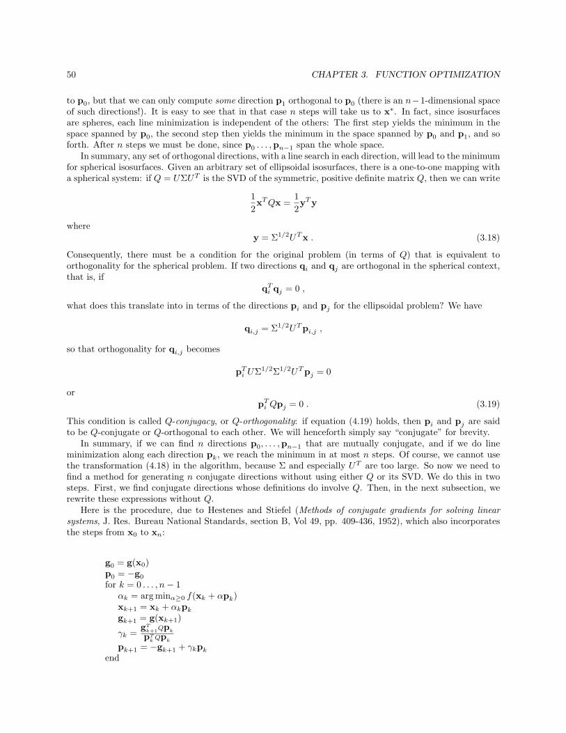
50 CHAPTER 3. FUNCTION OPTIMIZATION
to p0, but that we can only compute some direction p1 orthogonal to p0 (there is an n−1-dimensional spaceof such directions!). It is easy to see that in that case n steps will take us to x∗. In fact, since isosurfacesare spheres, each line minimization is independent of the others: The first step yields the minimum in thespace spanned by p0, the second step then yields the minimum in the space spanned by p0 and p1, and soforth. After n steps we must be done, since p0 . . . ,pn−1 span the whole space.
In summary, any set of orthogonal directions, with a line search in each direction, will lead to the minimumfor spherical isosurfaces. Given an arbitrary set of ellipsoidal isosurfaces, there is a one-to-one mapping witha spherical system: if Q = UΣUT is the SVD of the symmetric, positive definite matrix Q, then we can write
12xT Qx =
12yT y
wherey = Σ1/2UT x . (3.18)
Consequently, there must be a condition for the original problem (in terms of Q) that is equivalent toorthogonality for the spherical problem. If two directions qi and qj are orthogonal in the spherical context,that is, if
qTi qj = 0 ,
what does this translate into in terms of the directions pi and pj for the ellipsoidal problem? We have
qi,j = Σ1/2UT pi,j ,
so that orthogonality for qi,j becomes
pTi UΣ1/2Σ1/2UT pj = 0
orpT
i Qpj = 0 . (3.19)
This condition is called Q-conjugacy, or Q-orthogonality: if equation (4.19) holds, then pi and pj are saidto be Q-conjugate or Q-orthogonal to each other. We will henceforth simply say “conjugate” for brevity.
In summary, if we can find n directions p0, . . . ,pn−1 that are mutually conjugate, and if we do lineminimization along each direction pk, we reach the minimum in at most n steps. Of course, we cannot usethe transformation (4.18) in the algorithm, because Σ and especially UT are too large. So now we need tofind a method for generating n conjugate directions without using either Q or its SVD. We do this in twosteps. First, we find conjugate directions whose definitions do involve Q. Then, in the next subsection, werewrite these expressions without Q.
Here is the procedure, due to Hestenes and Stiefel (Methods of conjugate gradients for solving linearsystems, J. Res. Bureau National Standards, section B, Vol 49, pp. 409-436, 1952), which also incorporatesthe steps from x0 to xn:
g0 = g(x0)p0 = −g0
for k = 0 . . . , n− 1αk = arg minα≥0 f(xk + αpk)xk+1 = xk + αkpk
gk+1 = g(xk+1)
γk =gT
k+1Qpk
pTk
Qpk
pk+1 = −gk+1 + γkpk
end

3.3. CONJUGATE GRADIENTS 51
where
gk = g(xk) =∂f
∂x
∣∣∣∣x=xk
is the gradient of f at xk.It is simple to see that pk and pk+1 are conjugate. In fact,
pTk Qpk+1 = pT
k Q(−gk+1 + γkpk)
= −pTk Qgk+1 +
gTk+1Qpk
pTk Qpk
pTk Qpk
= −pTk Qgk+1 + gT
k+1Qpk = 0 .
It is somewhat more cumbersome to show that pi and pk+1 for i = 0, . . . , k are also conjugate. This can bedone by induction. The proof is based on the observation that the vectors pk are found by a generalizationof Gram-Schmidt (theorem 2.4.2) to produce conjugate rather than orthogonal vectors. Details can be foundin Polak’s book mentioned earlier.
3.3.2 Removing the Hessian
The algorithm shown in the previous subsection is a correct conjugate gradients algorithm. However, it iscomputationally inadequate because the expression for γk contains the Hessian Q, which is too large. Wenow show that γk can be rewritten in terms of the gradient values gk and gk+1 only. To this end, we noticethat
gk+1 = gk + αkQpk ,
orαkQpk = gk+1 − gk .
In fact,g(x) = a + Qx
so thatgk+1 = g(xk+1) = g(xk + αkpk) = a + Q(xk + αkpk) = gk + αkQpk .
We can therefore write
γk =gT
k+1Qpk
pTk Qpk
=gT
k+1αkQpk
pTk αkQpk
=gT
k+1(gk+1 − gk)pT
k (gk+1 − gk),
and Q has disappeared.This expression for γk can be further simplified by noticing that
pTk gk+1 = 0
because the line along pk is tangent to an isosurface at xk+1, while the gradient gk+1 is orthogonal to theisosurface at xk+1. Similarly,
pTk−1gk = 0 .
Then, the denominator of γk becomes
pTk (gk+1 − gk) = −pT
k gk = (gk − γk−1pk−1)T gk = gT
k gk .
In conclusion, we obtain the Polak-Ribiere formula
γk =gT
k+1(gk+1 − gk)gT
k gk
.

52 CHAPTER 3. FUNCTION OPTIMIZATION
3.3.3 Extension to General Functions
We now know how to minimize the quadratic function (4.16) in n steps, without ever constructing theHessian explicitly. When the function f(x) is arbitrary, the same algorithm can be used.
However, n iterations will not suffice. In fact, the Hessian, which was constant for the quadratic case,now is a function of xk. Strictly speaking, we then lose conjugacy, since pk and pk+1 are associated todifferent Hessians. However, as the algorithm approaches the minimum x∗, the quadratic approximationbecomes more and more valid, and a few cycles of n iterations each will achieve convergence.

CS 296.4
Mathematical Modelling of Continuous Systems
Carlo TomasiDuke University
Fall 2002

Chapter 5
Eigenvalues and Eigenvectors
Given a linear transformationb = Ax ,
the singular value decomposition A = UΣV T of A transforms the domain of the transformation via thematrix V T and its range via the matrix UT so that the transformed system is diagonal. In fact, the equationb = UΣV T x can be written as follows
UT b = ΣV T x ,
that is,c = Σy
where
y = V T x and c = UT b ,
and where Σ is diagonal. This is a fundamental transformation to use whenever the domain and the rangeof A are separate spaces. Often, however, domain and range are intimately related to one another evenindependently of the transformation A. The most important example is perhaps that of a system of lineardifferential equations, of the form
x = Ax
where A is n× n. For this equation, the fact that A is square is not a coincidence. In fact, x is assumed tobe a function of some real scalar variable t (often time), and x is the derivative of x with respect to t:
x =dxdt
.
In other words, there is an intimate, pre-existing relation between x and x, and one cannot change coordinatesfor x without also changing those for x accordingly. In fact, if V is an orthogonal matrix and we define
y = V T x ,
then the definition of x forces us to transform x by V T as well:
d V T xdt
= V T dxdt
= V T x .
In brief, the SVD does nothing useful for systems of linear differential equations, because it diagonalizesA by two different transformations, one for the domain and one for the range, while we need a singletransformation. Ideally, we would like to find an orthogonal matrix S and a diagonal matrix Λ such that
A = SΛST (5.1)
53

54 CHAPTER 5. EIGENVALUES AND EIGENVECTORS
so that if we definey = ST x
we can write the equivalent but diagonal differential system
y = Λy .
This is now much easier to handle, because it is a system of n independent, scalar differential equations,which can be solved separately. The solutions can then be recombined through
x = Sy .
We will see all of this in greater detail soon.Unfortunately, writing A in the form (5.1) is not always possible. This stands to reason, because now we
are imposing stronger constraints on the terms of the decomposition. It is like doing an SVD but with theadditional constraint U = V . If we refer back to figure 3.1, now the circle and the ellipse live in the samespace, and the constraint U = V implies that the vectors vi on the circle that map into the axes σiui of theellipse are parallel to the axes themselves. This will only occur for very special matrices.
In order to make a decomposition like (5.1) possible, we weaken the constraints in several ways:
• the elements of S and Λ are allowed to be complex, rather than real;
• the elements on the diagonal of Λ are allowed to be negative; in fact, they can be even non-real;
• S is required to be only invertible, rather than orthogonal.
To distinguish invertible from orthogonal matrices we use the symbol Q for invertible and S for orthogonal.In some cases, it will be possible to diagonalize A by orthogonal transformations S and ST . Finally, forcomplex matrices we generalize the notion of transpose by introducing the Hermitian operator: The matrixQH (pronounced “Q Hermitian”) is defined to be the complex conjugate of the transpose of Q. If Q happensto be real, conjugate transposition becomes simply transposition, so the Hermitian is a generalization of thetranspose. A matrix S is said to be unitary if
SHS = SSH = I ,
so unitary generalizes orthogonal for complex matrices. Unitary matrices merely rotate or flip vectors, inthe sense that they do not alter the vectors’ norms. For complex vectors, the norm squared is defined as
‖x‖2 = xHx ,
and if S is unitary we have‖Sx‖2 = xHSHSx = xHx = ‖x‖2 .
Furthermore, if x1 and x2 are mutually orthogonal, in the sense that
xH1 x2 = 0 ,
then Sx1 and Sx2 are orthogonal as well:
xH1 SHSx2 = xH
1 x2 = 0 .
In contrast, a nonunitary transformation Q can change the norms of vectors, as well as the inner productsbetween vectors. A matrix that is equal to its Hermitian is called a Hermitian matrix.
In summary, in order to diagonalize a square matrix A from a system of linear differential equations wegenerally look for a decomposition of A of the form
A = QΛQ−1 (5.2)

55
where Q and Λ are complex, Q is invertible, and Λ is diagonal. For some special matrices, this may specializeto
A = SΛSH
with unitary S.Whenever two matrices A and B, diagonal or not, are related by
A = QBQ−1 ,
they are said to be similar to each other, and the transformation of B into A (and vice versa) is called asimilarity transformation.
The equation A = QΛQ−1 can be rewritten as follows:
AQ = QΛ
or separately for every column of Q as follows:
Aqi = λiqi (5.3)
where
Q =[
q1 · · · qn
]and Λ = diag(λ1, . . . , λn) .
Thus, the columns of qi of Q and the diagonal entries λi of Λ are solutions of the eigenvalue/eigenvectorequation
Ax = λx , (5.4)
which is how eigenvalues and eigenvectors are usually introduced. In contrast, we have derived this equationfrom the requirement of diagonalizing a matrix by a similarity transformation. The columns of Q are calledeigenvectors, and the diagonal entries of Λ are called eigenvalues.
−2 −1 0 1 2−2
−1.5
−1
−0.5
0
0.5
1
1.5
2
Figure 5.1: Effect of the transformation (5.5) on a sample of points on the unit circle. The dashed lines arevectors that do not change direction under the transformation.
That real eigenvectors and eigenvalues do not always exist can be clarified by considering the eigenvalueproblem from a geometrical point of view in the n = 2 case. As we know, an invertible linear transformationtransforms the unit circle into an ellipse. Each point on the unit circle is transformed into some point onthe ellipse. Figure 5.1 shows the effect of the transformation represented by the matrix
A =[
2/3 4/√
30 2
](5.5)

56 CHAPTER 5. EIGENVALUES AND EIGENVECTORS
for a sample of points on the unit circle. Notice that there are many transformations that map the unitcircle into the same ellipse. In fact, the circle in figure 5.1 can be rotated, pulling the solid lines along.Each rotation yields another matrix A, but the resulting ellipse is unchanged. In other words, the curve-to-curve transformation from circle to ellipse is unique, but the point-to-point transformation is not. Matricesrepresent point-to-point transformations.
The eigenvalue problem amounts to finding axes q1,q2 that are mapped into themselves by the originaltransformation A (see equation (5.3)). In figure 5.1, the two eigenvectors are shown as dashed lines. Noticethat they do not correspond to the axes of the ellipse, and that they are not orthogonal. Equation (5.4) ishomogeneous in x, so x can be assumed to be a unit vector without loss of generality.
Given that the directions of the input vectors are generally changed by the transformation A, as evidentfrom figure 5.1, it is not obvious whether the eigenvalue problem admits a solution at all. We will see thatthe answer depends on the matrix A, and that a rather diverse array of situations may arise. In some cases,the eigenvalues and their eigenvectors exist, but they are complex. The geometric intuition is hidden, andthe problem is best treated as an algebraic one. In other cases, all eigenvalues exist, perhaps all real, butnot enough eigenvectors can be found, and the matrix A cannot be diagonalized. In particularly good cases,there are n real, orthonormal eigenvectors. In bad cases, we have to give up the idea of diagonalizing A, andwe can only triangularize it. This turns out to be good enough for solving linear differential systems, just astriangularization was sufficient for solving linear algebraic systems.
5.1 Computing Eigenvalues and Eigenvectors Algebraically
Let us rewrite the eigenvalue equationAx = λx
as follows:(A− λI)x = 0 . (5.6)
This is a homogeneous, square system of equations, which admits nontrivial solutions iff the matrix A− λIis rank-deficient. A square matrix B is rank-deficient iff its determinant,
det(B) ={
b11 if B is 1× 1∑ni=1(−1)i+1bi1 det(Bi1) otherwise
is zero. In this expression, Bij is the algebraic complement of entry bij , defined as the (n − 1) × (n − 1)matrix obtained by removing row i and column j from B.
Volumes have been written about the properties of the determinant. For our purposes, it is sufficient torecall the following properties from linear algebra:
• det(B) = det(BT );
• det([
b1 · · · bn
]) = 0 iff b1, . . . ,bn are linearly dependent;
• det([
b1 · · · bi · · · bj · · · bn
]) = − det(
[b1 · · · bj · · · bi · · · bn
]);
• det(BC) = det(B) det(C).
Thus, for system (5.6) to admit nontrivial solutions, we need
det(A− λI) = 0 . (5.7)
From the definition of determinant, it follows, by very simple induction, that the left-hand side of equation(5.7) is a polynomial of degree n in λ, and that the coefficient of λn is 1. Therefore, equation (5.7), whichis called the characteristic equation of A, has n complex solutions, in the sense that
det(A− λI) = (−1)n(λ− λ1) · . . . · (λ− λn)

5.1. COMPUTING EIGENVALUES AND EIGENVECTORS ALGEBRAICALLY 57
where some of the λi may coincide. In other words, an n×n matrix has at most n distinct eigenvalues. Thecase of exactly n distinct eigenvalues is of particular interest, because of the following results.
Theorem 5.1.1 Eigenvectors x1, . . . ,xk corresponding to distinct eigenvalues λ1, . . . , λk are linearly inde-pendent.
Proof. Suppose that c1x1 + . . .+ ckxk = 0 where the xi are eigenvectors of a matrix A. We need to showthat then c1 = . . . = ck = 0. By multiplying by A we obtain
c1Ax1 + . . . + ckAxk = 0
and because x1, . . . ,xk are eigenvectors corresponding to eigenvalues λ1, . . . , λk, we have
c1λ1x1 + . . . + ckλkxk = 0 . (5.8)
However, fromc1x1 + . . . + ckxk = 0
we also havec1λkx1 + . . . + ckλkxk = 0
and subtracting this equation from equation (5.8) we have
c1(λ1 − λk)x1 + . . . + ck−1(λk−1 − λk)xk−1 = 0 .
Thus, we have reduced the summation to one containing k−1 terms. Since all λi are distinct, the differencesin parentheses are all nonzero, and we can replace each xi by x′i = (λi − λk)xi, which is still an eigenvectorof A:
c1x′1 + . . . + ck−1x′k−1 = 0 .
We can repeat this procedure until only one term remains, and this forces c1 = 0, so that
c2x2 + . . . + ckxk = 0
This entire argument can be repeated for the last equation, therefore forcing c2 = 0, and so forth.In summary, the equation c1x1 + . . . + ckxk = 0 implies that c1 = . . . = ck = 0, that is, that the vectors
x1, . . . ,xk are linearly independent. ∆
For Hermitian matrices (and therefore for real symmetric matrices as well), the situation is even better.
Theorem 5.1.2 A Hermitian matrix has real eigenvalues.
Proof. A matrix A is Hermitian iff A = AH . Let λ and x be an eigenvalue of A and a correspondingeigenvector:
Ax = λx . (5.9)
By taking the Hermitian we obtainxHAH = λ∗xH .
Since A = AH , the last equation can be rewritten as follows:
xHA = λ∗xH . (5.10)
If we multiply equation (5.9) from the left by xH and equation (5.10) from the right by x, we obtain
xHAx = λxHx
xHAx = λ∗xHx

58 CHAPTER 5. EIGENVALUES AND EIGENVECTORS
which implies thatλxHx = λ∗xHx
Since x is an eigenvector, the scalar xHx is nonzero, so that we have
λ = λ∗
as promised. ∆
Corollary 5.1.3 A real and symmetric matrix has real eigenvalues.
Proof. A real and symmetric matrix is Hermitian. ∆
Theorem 5.1.4 Eigenvectors corresponding to distinct eigenvalues of a Hermitian matrix are mutuallyorthogonal.
Proof. Let λ and µ be two distinct eigenvalues of A, and let x and y be corresponding eigenvectors:
Ax = λx
Ay = µy ⇒ yHA = µyH
because A = AH and from theorem 5.1.2 µ = µ∗. If we multiply these two equations by yH from the leftand x from the right, respectively, we obtain
yHAx = λyHx
yHAx = µyHx ,
which impliesλyHx = µyHx
or(λ− µ)yHx = 0 .
Since the two eigenvalues are distinct, λ− µ is nonzero, and we must have yHx = 0. ∆
Corollary 5.1.5 An n×n Hermitian matrix with n distinct eigenvalues admits n orthonormal eigenvectors.
Proof. From theorem 5.1.4, the eigenvectors of an n×n Hermitian matrix with n distinct eigenvalues areall mutually orthogonal. Since the eigenvalue equation Ax = λx is homogeneous in x, the vector x can benormalized without violating the equation. Consequently, the eigenvectors can be made to be orthonormal.
∆
In summary, any square matrix with n distinct eigenvalues can be diagonalized by a similarity trans-formation, and any square Hermitian matrix with n distinct eigenvalues can be diagonalized by a unitarysimilarity transformation.
Notice that the converse is not true: a matrix can have coincident eigenvalues and still admit n indepen-dent, and even orthonormal, eigenvectors. For instance, the n × n identity matrix has n equal eigenvaluesbut n orthonormal eigenvectors (which can be chosen in infinitely many ways).
The examples in section 5.2 show that when some eigenvalues coincide, rather diverse situations canarise concerning the eigenvectors. First, however, we point out a simple but fundamental fact about theeigenvalues of a triangular matrix.

5.2. GOOD AND BAD MATRICES 59
Theorem 5.1.6 The determinant of a triangular matrix is the product of the elements on its diagonal.
Proof. This follows immediately from the definition of determinant. Without loss of generality, we canassume a triangular matrix B to be upper-triangular, for otherwise we can repeat the argument for thetranspose, which because of the properties above has the same eigenvalues. Then, the only possibly nonzerobi1 of the matrix B is b11, and the summation in the definition of determinant given above reduces to asingle term:
det(B) ={
b11 if B is 1× 1b11 det(B11) otherwise .
By repeating the argument for B11 and so forth until we are left with a single scalar, we obtain
det(B) = b11 · . . . · bnn .
∆
Corollary 5.1.7 The eigenvalues of a triangular matrix are the elements on its diagonal.
Proof. The eigenvalues of a matrix A are the solutions of the equation
det(A− λI) = 0 .
If A is triangular, so is B = A− λI, and from the previous theorem we obtain
det(A− λI) = (a11 − λ) · . . . · (ann − λ)
which is equal to zero forλ = a11, . . . , ann .
∆
Note that diagonal matrices are triangular, so this result holds for diagonal matrices as well.
5.2 Good and Bad Matrices
Solving differential equations becomes much easier when matrices have a full set of orthonormal eigenvectors.For instance, the matrix
A =[
2 00 1
](5.11)
has eigenvalues 2 and 1 and eigenvectors
s1 =[
10
]s2 =
[01
].
Matrices with n orthonormal eigenvectors are called normal. Normal matrices are good news, becausethen the n× n system of differential equations
x = Ax
has solution
x(t) =n∑
i=1
cisi eλit = S
eλ1t
. . .eλnt
c

60 CHAPTER 5. EIGENVALUES AND EIGENVECTORS
where S = [s1 · · · sn] are the eigenvectors, λi are the eigenvalues, and the vector c of constants ci is
c = SHx(0) .
More compactly,
x(t) = S
eλ1t
. . .eλnt
SHx(0) .
Fortunately these matrices occur frequently in practice. However, not all matrices are as good as these.First, there may still be a complete set of n eigenvectors, but they may not be orthonormal. An example ofsuch a matrix is [
2 −10 1
]
which has eigenvalues 2 and 1 and nonorthogonal eigenvectors
q1 =[
10
]q2 =
√2
2
[11
].
This is conceptually only a slight problem, because the unitary matrix S is replaced by an invertible matrixQ, and the solution becomes
x(t) = Q
eλ1t
. . .eλnt
Q−1x(0) .
Computationally this is more expensive, because a computation of a Hermitian is replaced by a matrixinversion.
However, things can be worse yet, and a full set of eigenvectors may fail to exist, as we now show.A necessary condition for an n×n matrix to be defective, that is, to have fewer than n eigenvectors, is that
it have repeated eigenvalues. In fact, we have seen (theorem 5.1.1) that a matrix with distinct eigenvalues(zero or nonzero does not matter) has a full set of eigenvectors (perhaps nonorthogonal, but independent).The simplest example of a defective matrix is
[0 10 0
]
which has double eigenvalue 0 and only eigenvector [1 0]T , while[
3 10 3
]
has double eigenvalue 3 and only eigenvector [1 0]T , so zero eigenvalues are not the problem.However, repeated eigenvalues are not a sufficient condition for defectiveness, as the identity matrix
proves.How bad can a matrix be? Here is a matrix that is singular, has fewer than n eigenvectors, and the
eigenvectors it has are not orthogonal. It belongs to the scum of all matrices:
A =
0 2 −10 2 10 0 2
.
Its eigenvalues are 0, because the matrix is singular, and 2, repeated twice. A has to have a repeatedeigenvalue if it is to be defective. Its two eigenvectors are
q1 =
100
, q2 =
√2
2
110

5.3. COMPUTING EIGENVALUES AND EIGENVECTORS NUMERICALLY 61
corresponding to eigenvalues 0 and 2 in this order, and there is no q3. Furthermore, q1 and q2 are notorthogonal to each other.
5.3 Computing Eigenvalues and Eigenvectors Numerically
The examples above have shown that not every n × n matrix admits n independent eigenvectors, so somematrices cannot be diagonalized by similarity transformations. Fortunately, these matrices can be triangu-larized by similarity transformations, as we now show. We will show later on that this allows solving systemsof linear differential equations regardless of the structure of the system’s matrix of coefficients.
It is important to notice that if a matrix A is triangularized by similarity transformations,
T = Q−1AQ ,
then the eigenvalues of the triangular matrix T are equal to those of the original matrix A. In fact, if
Ax = λx ,
thenQTQ−1x = λx ,
that is,Ty = λy
wherey = Q−1x ,
so λ is also an eigenvalue for T . The eigenvectors, however, are changed according to the last equation.The Schur decomposition does even better, since it triangularizes any square matrix A by a unitary
(possibly complex) transformation:T = SHAS .
This transformation is equivalent to factoring A into the product
A = STSH ,
and this product is called the Schur decomposition of A. Numerically stable and efficient algorithms existfor the Schur decomposition. In this note, we will not study these algorithms, but only show that all squarematrices admit a Schur decomposition.
5.3.1 Rotations into the x1 Axis
An important preliminary fact concerns vector rotations. Let e1 be the first column of the identity matrix.It is intuitively obvious that any nonzero real vector x can be rotated into a vector parallel to e1. Formally,take any orthogonal matrix S whose first column is
s1 =x‖x‖ .
Since sT1 x = xT x/‖x‖ = ‖x‖, and since all the other sj are orthogonal to s1, we have
ST x =
sT1...
sTn
x =
sT1 x...
sTnx
=
‖x‖0...0

62 CHAPTER 5. EIGENVALUES AND EIGENVECTORS
which is parallel to e1 as desired. It may be less obvious that a complex vector x can be transformed into areal vector parallel to e1 by a unitary transformation. But the trick is the same: let
s1 =x‖x‖ .
Now s1 may be complex. We have sH1 x = xHx/‖x‖ = ‖x‖, and
SHx =
sH1...
sHn
x =
sH1 x...
sHn x
=
‖x‖0...0
,
just about like before. We are now ready to triangularize an arbitrary square matrix A.
5.3.2 The Schur Decomposition
The Schur decomposition theorem is the cornerstone of eigenvalue computations. It states that any squarematrix can be triangularized by unitary transformations. The diagonal elements of a triangular matrix areits eigenvalues, and unitary transformations preserve eigenvalues. Consequently, if the Schur decompositionof a matrix can be computed, its eigenvalues can be determined. Moreover, as we will see later, a system oflinear differential equations can be solved regardless of the structure of the matrix of its coefficients.
Lemma 5.3.1 If A is an n×n matrix and λ and x are an eigenvalue of A and its corresponding eigenvector,
Ax = λx (5.12)
then there is a transformationT = UHAU
where U is a unitary, n× n matrix, such that
T =
λ0...0
C
.
Proof. Let U be a unitary transformation that transforms the (possibly complex) eigenvector x of A intoa real vector on the x1 axis:
x = U
r0...0
where r is the nonzero norm of x. By substituting this into (5.12) and rearranging we have
AU
r0...0
= λU
r0...0
UHAU
r0...0
= λ
r0...0

5.3. COMPUTING EIGENVALUES AND EIGENVECTORS NUMERICALLY 63
UHAU
10...0
= λ
10...0
T
10...0
=
λ0...0
.
The last left-hand side is the first column of T , and the corresponding right-hand side is of the form requiredby the lemma. ∆
Theorem 5.3.2 (Schur) If A is any n× n matrix then there exists a unitary n× n matrix S such that
SHAS = T
where T is triangular. Furthermore, S can be chosen so that the eigenvalues λi of A appear in any orderalong the diagonal of T .
Proof. By induction. The theorem obviously holds for n = 1:
1 A 1 = A .
Suppose it holds for all matrices of order n− 1. Then from the lemma there exists a unitary U such that
UHAU =
λ0...0
C
where λ is any eigenvalue of A. Partition C into a row vector and an (n− 1)× (n− 1) matrix G:
C =[
wH
G
].
By the inductive hypothesis, there is a unitary matrix V such that V HGV is a Schur decomposition of G.Let
S = U
1 0 · · · 00...0
V
.
Clearly, S is a unitary matrix, and SHAS is upper-triangular. Since the elements on the diagonal of atriangular matrix are the eigenvalues, SHAS is the Schur decomposition of A. Because we can pick anyeigenvalue as λ, the order of eigenvalues can be chosen arbitrarily. ∆
This theorem does not say how to compute the Schur decomposition, only that it exists. Fortunately,there is a stable and efficient algorithm to compute the Schur decomposition. This is the preferred way tocompute eigenvalues numerically.

64 CHAPTER 5. EIGENVALUES AND EIGENVECTORS
5.4 Eigenvalues/Vectors and Singular Values/Vectors
In this section we prove a few additional important properties of eigenvalues and eigenvectors. In the process,we also establish a link between singular values/vectors and eigenvalues/vectors. While this link is veryimportant, it is useful to remember that eigenvalues/vectors and singular values/vectors are conceptuallyand factually very distinct entities (recall figure 5.1).
First, a general relation between determinant and eigenvalues.
Theorem 5.4.1 The determinant of a matrix is equal to the product of its eigenvalues.
Proof. The proof is very simple, given the Schur decomposition. In fact, we know that the eigenvalues ofa matrix A are equal to those of the triangular matrix in the Schur decomposition of A. Furthermore, weknow from theorem 5.1.6 that the determinant of a triangular matrix is the product of the elements on itsdiagonal. If we recall that a unitary matrix has determinant 1 or -1, that the determinants of S and SH arethe same, and that the determinant of a product of matrices is equal to the product of the determinants,the proof is complete. ∆
We saw that an n × n Hermitian matrix with n distinct eigenvalues admits n orthonormal eigenvectors(corollary 5.1.5). The assumption of distinct eigenvalues made the proof simple, but is otherwise unnecessary.In fact, now that we have the Schur decomposition, we can state the following stronger result.
Theorem 5.4.2 (Spectral theorem) Every Hermitian matrix can be diagonalized by a unitary matrix,and every real symmetric matrix can be diagonalized by an orthogonal matrix:
A = AH ⇒ A = SΛSH
A real, A = AT ⇒ A = SΛST , S real .
In either case, Λ is real and diagonal.
Proof. We already know that Hermitian matrices (and therefore real and symmetric ones) have realeigenvalues (theorem 5.1.2), so Λ is real. Let now
A = STSH
be the Schur decomposition of A. Since A is Hermitian, so is T . In fact, T = SHAS, and
TH = (SHAS)H = SHAHS = SHAS = T .
But the only way that T can be both triangular and Hermitian is for it to be diagonal, because 0∗ = 0. Thus,the Schur decomposition of a Hermitian matrix is in fact a diagonalization, and this is the first equation ofthe theorem (the diagonal of a Hermitian matrix must be real).
Let now A be real and symmetric. All that is left to prove is that then its eigenvectors are real. Buteigenvectors are the solution of the homogeneous system (5.6), which is both real and rank-deficient, andtherefore admits nontrivial real solutions. Thus, S is real, and SH = ST . ∆
In other words, a Hermitian matrix, real or not, with distinct eigenvalues or not, has real eigenvalues andn orthonormal eigenvectors. If in addition the matrix is real, so are its eigenvectors.
We recall that a real matrix A such that for every nonzero x we have xT Ax > 0 is said to be positivedefinite. It is positive semidefinite if for every nonzero x we have xT Ax ≥ 0. Notice that a positivedefinite matrix is also positive semidefinite. Positive definite or semidefinite matrices arise in the solution of

5.4. EIGENVALUES/VECTORS AND SINGULAR VALUES/VECTORS 65
overconstrained linear systems, because AT A is positive semidefinite for every A (lemma 5.4.5). They alsooccur in geometry through the equation of an ellipsoid,
xT Qx = 1
in which Q is positive definite. In physics, positive definite matrices are associated to quadratic forms xT Qxthat represent energies or second-order moments of mass or force distributions. Their physical meaningmakes them positive definite, or at least positive semidefinite (for instance, energies cannot be negative). Thefollowing result relates eigenvalues/vectors with singular values/vectors for positive semidefinite matrices.
Theorem 5.4.3 The eigenvalues of a real, symmetric, positive semidefinite matrix A are equal to its singularvalues. The eigenvectors of A are also its singular vectors, both left and right.
Proof. From the previous theorem, A = SΛST , where both Λ and S are real. Furthermore, the entriesin Λ are nonnegative. In fact, from
Asi = λsi
we obtainsTi Asi = sT
i λsi = λsTi si = λ‖si‖2 = λ .
If A is positive semidefinite, then xT Ax ≥ 0 for any nonzero x, and in particular sTi Asi ≥ 0, so that λ ≥ 0.
ButA = SΛST
with nonnegative diagonal entries in Λ is the singular value decomposition A = UΣV T of A with Σ = Λ andU = V = S. Recall that the eigenvalues in the Schur decomposition can be arranged in any desired orderalong the diagonal. ∆
Theorem 5.4.4 A real, symmetric matrix is positive semidefinite iff all its eigenvalues are nonnegative. Itis positive definite iff all its eigenvalues are positive.
Proof. Theorem 5.4.3 implies one of the two directions: If A is real, symmetric, and positive semidefinite,then its eigenvalues are nonnegative. If the proof of that theorem is repeated with the strict inequality, wealso obtain that if A is real, symmetric, and positive definite, then its eigenvalues are positive.
Conversely, we show that if all eigenvalues λ of a real and symmetric matrix A are positive (nonnegative)then A is positive definite (semidefinite). To this end, let x be any nonzero vector. Since real and symmetricmatrices have n orthonormal eigenvectors (theorem 5.4.2), we can use these eigenvectors s1, . . . , sn as anorthonormal basis for Rn, and write
x = c1s1 + . . . + cnsn
withci = xT si .
But then
xT Ax = xT A(c1s1 + . . . + cnsn) = xT (c1As1 + . . . + cnAsn)= xT (c1λ1s1 + . . . + cnλnsn) = c1λ1xT s1 + . . . + cnλnxT sn
= λ1c21 + . . . + λnc2
n > 0 (or ≥ 0)
because the λi are positive (nonnegative) and not all ci can be zero. Since xT Ax > 0 (or ≥ 0) for everynonzero x, A is positive definite (semidefinite). ∆
Theorem 5.4.3 establishes one connection between eigenvalues/vectors and singular values/vectors: forsymmetric, positive definite matrices, the concepts coincide. This result can be used to introduce a lessdirect link, but for arbitrary matrices.

66 CHAPTER 5. EIGENVALUES AND EIGENVECTORS
Lemma 5.4.5 AT A is positive semidefinite.
Proof. For any nonzero x we can write xT AT Ax = ‖Ax‖2 ≥ 0. ∆
Theorem 5.4.6 The eigenvalues of AT A with m ≥ n are the squares of the singular values of A; theeigenvectors of AT A are the right singular vectors of A. Similarly, for m ≤ n, the eigenvalues of AAT arethe squares of the singular values of A, and the eigenvectors of AAT are the left singular vectors of A.
Proof. If m ≥ n and A = UΣV T is the SVD of A, we have
AT A = V ΣUT UΣV T = V Σ2V T
which is in the required format to be a (diagonal) Schur decomposition with S = V and T = Λ = Σ2.Similarly, for m ≤ n,
AAT = UΣV T V ΣUT = UΣ2UT
is a Schur decomposition with S = U and T = Λ = Σ2. ∆
We have seen that important classes of matrices admit a full set of orthonormal eigenvectors. The theorembelow characterizes the class of all matrices with this property, that is, the class of all normal matrices. Toprove the theorem, we first need a lemma.
Lemma 5.4.7 If for an n × n matrix B we have BBH = BHB, then for every i = 1, . . . , n, the norm ofthe i-th row of B equals the norm of its i-th column.
Proof. From BBH = BHB we deduce
‖Bx‖2 = xHBHBx = xHBBHx = ‖BHx‖2 . (5.13)
If x = ei, the i-th column of the n × n identity matrix, Bei is the i-th column of B, and BHei is the i-thcolumn of BH , which is the conjugate of the i-th row of B. Since conjugation does not change the norm ofa vector, the equality (5.13) implies that the i-th column of B has the same norm as the i-th row of B. ∆
Theorem 5.4.8 An n× n matrix is normal if an only if it commutes with its Hermitian:
AAH = AHA .
Proof. Let A = STSH be the Schur decomposition of A. Then,
AAH = STSHSTHSH = STTHSH and AHA = STHSHSTSH = STHTSH .
Because S is invertible (even unitary), we have AAH = AHA if and only if TTH = THT .However, a triangular matrix T for which TTH = THT must be diagonal. In fact, from the lemma, the
norm of the i-th row of T is equal to the norm of its i-th column. Let i = 1. Then, the first column of Thas norm |t11|. The first row has first entry t11, so the only way that its norm can be |t11| is for all otherentries in the first row to be zero. We now proceed through i = 2, . . . , n, and reason similarly to concludethat T must be diagonal.
The converse is also obviously true: if T is diagonal, then TTH = THT . Thus, AAH = AHA if and onlyif T is diagonal, that is, if and only if A can be diagonalized by a unitary similarity transformation. This isthe definition of a normal matrix. ∆

5.4. EIGENVALUES/VECTORS AND SINGULAR VALUES/VECTORS 67
Corollary 5.4.9 A triangular, normal matrix must be diagonal.
Proof. We proved this in the proof of theorem 5.4.8. ∆
Checking that AHA = AAH is much easier than computing eigenvectors, so theorem 5.4.8 is a very usefulcharacterization of normal matrices. Notice that Hermitian (and therefore also real symmetric) matricescommute trivially with their Hermitians, but so do, for instance, unitary (and therefore also real orthogonal)matrices:
UUH = UHU = I .
Thus, Hermitian, real symmetric, unitary, and orthogonal matrices are all normal.

CS 296.4
Mathematical Modelling of Continuous Systems
Carlo TomasiDuke University
Fall 2002

68

Chapter 6
Ordinary Differential Systems
In this chapter we use the theory developed in chapter 5 in order to solve systems of first-order lineardifferential equations with constant coefficients. These systems have the following form:
x = Ax + b(t) (6.1)x(0) = x0 (6.2)
where x = x(t) is an n-dimensional vector function of time t, the dot denotes differentiation, the coefficientsaij in the n × n matrix A are constant, and the vector function b(t) is a function of time. The equation(6.2), in which x0 is a known vector, defines the initial value of the solution.
First, we show that scalar differential equations of order greater than one can be reduced to systems offirst-order differential equations. Then, in section 6.2, we recall a general result for the solution of first-orderdifferential systems from the elementary theory of differential equations. In section 6.3, we make this resultmore specific by showing that the solution to a homogeneous system is a linear combination of exponentialsmultiplied by polynomials in t. This result is based on the Schur decomposition introduced in chapter 5,which is numerically preferable to the more commonly used Jordan canonical form. Finally, in sections 6.4and 6.5, we set up and solve a particular differential system as an illustrative example.
6.1 Scalar Differential Equations of Order Higher than One
The first-order system (6.1) subsumes also the case of a scalar differential equation of order n, possiblygreater than 1,
dny
dtn+ cn−1
dn−1y
dtn−1+ . . . + c1
dy
dt+ c0y = b(t) . (6.3)
In fact, such an equation can be reduced to a first-order system of the form (6.1) by introducing the n-dimensional vector
x =
x1
...xn
=
ydydt...
dn−1ydtn−1
.
With this definition, we have
diy
dti= xi+1 for i = 0, . . . , n− 1
dny
dtn=
dxn
dt,
69

70 CHAPTER 6. ORDINARY DIFFERENTIAL SYSTEMS
and x satisfies the additional n− 1 equations
xi+1 =dxi
dt(6.4)
for i = 1, . . . , n− 1. If we write the original system (6.3) together with the n− 1 differential equations (6.4),we obtain the first-order system
x = Ax + b(t)
where
A =
0 1 0 · · · 00 0 1 · · · 0...
......
. . ....
0 0 0 · · · 1−c0 −c1 −c2 · · · −cn−1
is the so-called companion matrix of (6.3) and
b(t) =
00...0
b(t)
.
6.2 General Solution of a Linear Differential System
We know from the general theory of differential equations that a general solution of system (6.1) with initialcondition (6.2) is given by
x(t) = xh(t) + xp(t)
where xh(t) is the solution of the homogeneous system
x = Ax
x(0) = x0
and xp(t) is a particular solution of
x = Ax + b(t)x(0) = 0 .
The two solution components xh and xp can be written by means of the matrix exponential, introduced inthe following.
For the scalar exponential eλt we can write a Taylor series expansion
eλt = 1 +λt
1!+
λ2t2
2!+ · · · =
∞∑
j=0
λjtj
j!.
Usually1, in calculus classes, the exponential is introduced by other means, and the Taylor series expansionabove is proven as a property.
For matrices, the exponential eZ of a matrix Z ∈ Rn×n is instead defined by the infinite series expansion
eZ = I +Z
1!+
Z2
2!+ · · · =
∞∑
j=0
Zj
j!.
1Not always. In some treatments, the exponential is defined through its Taylor series.

6.2. GENERAL SOLUTION OF A LINEAR DIFFERENTIAL SYSTEM 71
Here I is the n × n identity matrix, and the general term Zj/j! is simply the matrix Z raised to the jthpower divided by the scalar j!. It turns out that this infinite sum converges (to an n × n matrix which wewrite as eZ) for every matrix Z. Substituting Z = At gives
eAt = I +At
1!+
A2t2
2!+
A3t3
3!+ · · · =
∞∑
j=0
Ajtj
j!. (6.5)
Differentiating both sides of (6.5) gives
deAt
dt= A +
A2t
1!+
A3t2
2!+ · · ·
= A
(I +
At
1!+
A2t2
2!+ · · ·
)
deAt
dt= AeAt.
Thus, for any vector w, the function xh(t) = eAtw satisfies the homogeneous differential system
xh = Axh .
By using the initial values (6.2) we obtain v = x0, and
xh(t) = eAtx(0) (6.6)
is a solution to the differential system (6.1) with b(t) = 0 and initial values (6.2). It can be shown that thissolution is unique.
From the elementary theory of differential equations, we also know that a particular solution to thenonhomogeneous (b(t) 6= 0) equation (6.1) is given by
xp(t) =∫ t
0
eA(t−s) b(s) ds .
This is easily verified, since by differentiating this expression for xp we obtain
xp = AeAt
∫ t
0
e−As b(s) ds + eAt e−At b(t) = Axp + b(t) ,
so xp satisfies equation (6.1).In summary, we have the following result.
The solution tox = Ax + b(t) (6.7)
with initial valuex(0) = x0 (6.8)
isx(t) = xh(t) + xp(t) (6.9)
wherexh(t) = eAtx(0) (6.10)
and
xp(t) =∫ t
0
eA(t−s) b(s) ds . (6.11)

72 CHAPTER 6. ORDINARY DIFFERENTIAL SYSTEMS
Since we now have a formula for the general solution to a linear differential system, we seem to have allwe need. However, we do not know how to compute the matrix exponential. The naive solution to use thedefinition (6.5) requires too many terms for a good approximation. As we have done for the SVD and theSchur decomposition, we will only point out that several methods exist for computing a matrix exponential,but we will not discuss how this is done2. In a fundamental paper on the subject, Nineteen dubious ways tocompute the exponential of a matrix (SIAM Review, vol. 20, no. 4, pp. 801-36), Cleve Moler and CharlesVan Loan discuss a large number of different methods, pointing out that no one of them is appropriate forall situations. A full discussion of this matter is beyond the scope of these notes.
When the matrix A is constant, as we currently assume, we can be much more specific about the structureof the solution (6.9) of system (6.7), and particularly so about the solution xh(t) to the homogeneous part.Specifically, the matrix exponential (6.10) can be written as a linear combination, with constant vectorcoefficients, of scalar exponentials multiplied by polynomials. In the general theory of linear differentialsystems, this is shown via the Jordan canonical form. However, in the paper cited above, Moler and VanLoan point out that the Jordan form cannot be computed reliably, and small perturbations in the data canchange the results dramatically. Fortunately, a similar result can be found through the Schur decompositionintroduced in chapter 5. The next section shows how to do this.
6.3 Structure of the Solution
For the homogeneous case b(t) = 0, consider the first order system of linear differential equations
x = Ax (6.12)x(0) = x0 . (6.13)
Two cases arise: either A admits n distinct eigenvalues, or is does not. In chapter 5, we have seen thatif (but not only if) A has n distinct eigenvalues then it has n linearly independent eigenvectors (theorem5.1.1), and we have shown how to find xh(t) by solving an eigenvalue problem. In section 6.3.1, we brieflyreview this solution. Then, in section 6.3.2, we show how to compute the homogeneous solution xh(t) in theextreme case of an n× n matrix A with n coincident eigenvalues.
To be sure, we have seen that matrices with coincident eigenvalues can still have a full set of linearlyindependent eigenvectors (see for instance the identity matrix). However, the solution procedure we introducein section 6.3.2 for the case of n coincident eigenvalues can be applied regardless to how many linearlyindependent eigenvectors exist. If the matrix has a full complement of eigenvectors, the solution obtained insection 6.3.2 is the same as would be obtained with the method of section 6.3.1.
Once these two extreme cases (nondefective matrix or all-coincident eigenvalues) have been handled, weshow a general procedure in section 6.3.3 for solving a homogeneous or nonhomogeneous differential systemfor any, square, constant matrix A, defective or not. This procedure is based on backsubstitution, andproduces a result analogous to that obtained via Jordan decomposition for the homogeneous part xh(t) ofthe solution. However, since it is based on the numerically sound Schur decomposition, the method of section6.3.3 is superior in practice. For a nonhomogeneous system, the procedure can be carried out analytically ifthe functions in the right-hand side vector b(t) can be integrated.
6.3.1 A is Not Defective
In chapter 5 we saw how to find the homogeneous part xh(t) of the solution when A has a full set of nlinearly independent eigenvectors. This result is briefly reviewed in this section for convenience.3
If A is not defective, then it has n linearly independent eigenvectors q1, . . . ,qn with correspondingeigenvalues λ1, . . . , λn. Let
Q =[
q1 · · · qn
].
2In Matlab, expm(A) is the matrix exponential of A.3Parts of this subsection and of the following one are based on notes written by Scott Cohen.

6.3. STRUCTURE OF THE SOLUTION 73
This square matrix is invertible because its columns are linearly independent. Since Aqi = λiqi, we have
AQ = QΛ, (6.14)
where Λ = diag(λ1, . . . , λn) is a square diagonal matrix with the eigenvalues of A on its diagonal. Multiplyingboth sides of (6.14) by Q−1 on the right, we obtain
A = QΛQ−1. (6.15)
Then, system (6.12) can be rewritten as follows:
x = Ax
x = QΛQ−1x
Q−1x = ΛQ−1x
y = Λy, (6.16)
where y = Q−1x. The last equation (6.16) represents n uncoupled, homogeneous, differential equationsyi = λiyi. The solution is
yh(t) = eΛty(0),
whereeΛt = diag(eλ1t, . . . , eλnt).
Using the relation x = Qy, and the consequent relation y(0) = Q−1x(0), we see that the solution to thehomogeneous system (6.12) is
xh(t) = QeΛtQ−1x(0).
If A is normal, that is, if it has n orthonormal eigenvectors q1, . . . qn, then Q is replaced by the Hermitianmatrix S =
[s1 · · · sn
], Q−1 is replaced by SH , and the solution to (6.12) becomes
xh(t) = SeΛtSHx(0).
6.3.2 A Has n Coincident Eigenvalues
When A = QΛQ−1, we derived that the solution to (6.12) is xh(t) = QeΛtQ−1x(0). Comparing with (6.6),it should be the case that
eQ(Λt)Q−1= QeΛtQ−1.
This follows easily from the definition of eZ and the fact that (Q(Λt)Q−1)j = Q(Λt)jQ−1. Similarly, ifA = SΛSH , where S is Hermitian, then the solution to (6.12) is xh(t) = SeΛtSHx(0), and
eS(Λt)SH
= SeΛtSH .
How can we compute the matrix exponential in the extreme case in which A has n coincident eigen-values, regardless of the number of its linearly independent eigenvectors? In any case, A admits a Schurdecomposition
A = STSH
(theorem 5.3.2). We recall that S is a unitary matrix and T is upper triangular with the eigenvalues of Aon its diagonal. Thus we can write T as
T = Λ + N,
where Λ is diagonal and N is strictly upper triangular. The solution (6.6) in this case becomes
xh(t) = eS(Tt)SH
x(0) = SeTtSHx(0) = SeΛt+NtSHx(0).

74 CHAPTER 6. ORDINARY DIFFERENTIAL SYSTEMS
Thus we can compute (6.6) if we can compute eTt = eΛt+Nt. This turns out to be almost as easy ascomputing eΛt when the diagonal matrix Λ is a multiple of the identity matrix:
Λ = λ I
that is, when all the eigenvalues of A coincide. In fact, in this case, Λt and Nt commute:
Λt Nt = λ It Nt = λtNt = Nt λt = Ntλ It = Nt Λt .
It can be shown that if two matrices Z1 and Z2 commute, that is if
Z1Z2 = Z2Z1 ,
theneZ1+Z2 = eZ1eZ2 = eZ2eZ1 .
Thus, in our case, we can writeeΛt+Nt = eΛteNt.
We already know how to compute eΛt, so it remains to show how to compute eNt. The fact that Nt isstrictly upper triangular makes the computation of this matrix exponential much simpler than for a generalmatrix Z.
Suppose, for example, that N is 4 × 4. Then N has three nonzero superdiagonals, N2 has two nonzerosuperdiagonals, N3 has one nonzero superdiagonal, and N4 is the zero matrix:
N =
0 ∗ ∗ ∗0 0 ∗ ∗0 0 0 ∗0 0 0 0
→ N2 =
0 0 ∗ ∗0 0 0 ∗0 0 0 00 0 0 0
→
N3 =
0 0 0 ∗0 0 0 00 0 0 00 0 0 0
→ N4 =
0 0 0 00 0 0 00 0 0 00 0 0 0
.
In general, for a strictly upper triangular n× n matrix, we have N j = 0 for all j ≥ n (i.e., N is nilpotent oforder n). Therefore,
eNt =∞∑
j=0
N jtj
j!=
n−1∑
j=0
N jtj
j!
is simply a finite sum, and the exponential reduces to a matrix polynomial.In summary, the general solution to the homogeneous differential system (6.12) with initial value (6.13)
when the n× n matrix A has n coincident eigenvalues is given by
xh(t) = SeΛtn−1∑
j=0
N jtj
j!SHx0 (6.17)
whereA = S(Λ + N)SH
is the Schur decomposition of A,Λ = λ I
is a multiple of the identity matrix containing the coincident eigenvalues of A on its diagonal, and N isstrictly upper triangular.

6.3. STRUCTURE OF THE SOLUTION 75
6.3.3 The General Case
We are now ready to solve the linear differential system
x = Ax + b(t) (6.18)x(0) = x0 (6.19)
in the general case of a constant matrix A, defective or not, with arbitrary b(t). In fact, let A = STSH bethe Schur decomposition of A, and consider the transformed system
y(t) = Ty(t) + c(t) (6.20)
where
y(t) = SHx(t) and c(t) = SHb(t) . (6.21)
The triangular matrix T can always be written in the following form:
T =
T11 · · · · · · T1k
0 T22 · · · T2k
.... . .
...0 · · · 0 Tkk
where the diagonal blocks Tii for i = 1, . . . , k are of size ni × ni (possibly 1 × 1) and contain all-coincidenteigenvalues. The remaining nonzero blocks Tij with i < j can be in turn bundled into matrices
Ri =[
Ti,i+1 · · · Ti,k
]
that contain everything to the right of the corresponding Tii. The vector c(t) can be partitioned correspond-ingly as follows
c(t) =
c1(t)...
ck(t)
where ci has ni entries, and the same can be done for
y(t) =
y1(t)...
yk(t)
and for the initial values
y(0) =
y1(0)...
yk(0)
.
The triangular system (6.20) can then be solved by backsubstitution as follows:
for i = k down to 1if i < k
di(t) = Ri[yi+1(t), . . . ,yk(t)]T
elsedi(t) = 0 (an nk-dimensional vector of zeros)
endTii = λi I + Ni (diagonal and strictly upper-triangular part of Tii)
yi(t) = eλiIt∑ni−1
j=0Nj
itj
j! yi(0) +∫ t
0
(eλiI(t−s)
∑ni−1j=0
Nji(t−s)j
j!
)(ci(s) + di(s)) ds
end.

76 CHAPTER 6. ORDINARY DIFFERENTIAL SYSTEMS
In this procedure, the expression for yi(t) is a direct application of equations (6.9), (6.10), (6.11), and(6.17) with S = I. In the general case, the applicability of this routine depends on whether the integral inthe expression for yi(t) can be computed analytically. This is certainly the case when b(t) is a constantvector b, because then the integrand is a linear combination of exponentials multiplied by polynomials int− s, which can be integrated by parts.
The solution x(t) for the original system (6.18) is then
x(t) = Sy(t) .
As an illustration, we consider a very small example, the 2× 2 homogeneous, triangular case,[
y1
y2
]=
[t11 t120 t22
] [y1
y2
]. (6.22)
When t11 = t22 = λ, we obtain
y(t) = eλIt
[1 t12t0 1
]y(0) .
In scalar form, this becomes
y1(t) = (y1(0) + t12y2(0) t) eλt
y2(t) = y2(0) eλt ,
and it is easy to verify that this solution satisfies the differential system (6.22).When t11 = λ1 6= t22 = λ2, we could solve the system by finding the eigenvectors of T , since we
know that in this case two linearly independent eigenvectors exist (theorem 5.1.1). Instead, we apply thebacksubstitution procedure introduced in this section. The second equation of the system,
y2(t) = t22y2
has solutiony2(t) = y2(0) eλ2t .
We then haved1(t) = t12y2(t) = t12y2(0) eλ2t
and
y1(t) = y1(0)eλ1t +∫ t
0
eλ1(t−s)d1(s) ds
= y1(0)eλ1t + t12y2(0) eλ1t
∫ t
0
e−λ1seλ2s ds
= y1(0)eλ1t + t12y2(0) eλ1t
∫ t
0
e(λ2−λ1)s ds
= y1(0)eλ1t +t12y2(0)λ2 − λ1
eλ1t(e(λ2−λ1)t − 1)
= y1(0)eλ1t +t12y2(0)λ2 − λ1
(eλ2t − eλ1t)
Exercise: verify that this solution satisfies both the differential equation (6.22) and the initial value equationy(0) = y0.
Thus, the solutions to system (6.22) for t11 = t22 and for t11 6= t22 have different forms. While y2(t) isthe same in both cases, we have
y1(t) = y1(0) eλt + t12y2(0) t eλt if t11 = t22
y1(t) = y1(0)eλ1t +t12y2(0)λ2 − λ1
(eλ2t − eλ1t) if t11 6= t22 .
6.4. A CONCRETE EXAMPLE 77
rest positionof mass 1
rest positionof mass 2
2v
1v
1
2
2
1
3
Figure 6.1: A system of masses and springs. In the absence of external forces, the two masses would assumethe positions indicated by the dashed lines.
This would seem to present numerical difficulties when t11 ≈ t22, because the solution would suddenlyswitch from one form to the other as the difference between t11 and t22 changes from about zero to exactlyzero or viceversa. This, however, is not a problem. In fact,
limλ1→λ
eλt − eλ1t
λ− λ1= t eλt ,
and the transition between the two cases is smooth.
6.4 A Concrete Example
In this section we set up and solve a more concrete example of a system of differential equations. The initialsystem has two second-order equations, and is transformed into a first-order system with four equations.The 4× 4 matrix of the resulting system has an interesting structure, which allows finding eigenvalues andeigenvectors analytically with a little trick. The point of this section is to show how to transform the complexformal solution of the differential system, computed with any of the methods described above, into a realsolution in a form appropriate to the problem at hand.
Consider the mechanical system in figure 6.1. Suppose that we want to study the evolution of the systemover time. Since forces are proportional to accelerations, because of Newton’s law, and since accelerationsare second derivatives of position, the new equations are differential. Because differentiation occurs onlywith respect to one variable, time, these are ordinary differential equations, as opposed to partial.
In the following we write the differential equations that describe this system. Two linear differentialequations of the second order4 result. We will then transform these into four linear differential equations ofthe first order.
4Recall that the order of a differential equation is the highest degree of derivative that appears in it.
78 CHAPTER 6. ORDINARY DIFFERENTIAL SYSTEMS
By Hooke’s law, the three springs exert forces that are proportional to the springs’ elongations:
f1 = c1v1
f2 = c2(v2 − v1)f3 = −c3v2
where the ci are the positive spring constants (in newtons per meter).The accelerations of masses 1 and 2 (springs are assumed to be massless) are proportional to their
accelerations, according to Newton’s second law:
m1v1 = −f1 + f2 = −c1v1 + c2(v2 − v1) = −(c1 + c2)v1 + c2v2
m2v2 = −f2 + f3 = −c2(v2 − v1)− c3v2 = c2v1 − (c2 + c3)v2
or, in matrix form,v = Bv (6.23)
where
v =[
v1
v2
]and B =
[ − c1+c2m1
c2m1
c2m2
− c2+c3m2
].
We also assume that initial conditions
v(0) and v(0) (6.24)
are given, which specify positions and velocities of the two masses at time t = 0.To solve the second-order system (6.23), we will first transform it to a system of four first-order equations.
As shown in the introduction to this chapter, the trick is to introduce variables to denote the first-orderderivatives of v, so that second-order derivatives of v are first-order derivatives of the new variables. Foruniformity, we define four new variables
u =
u1
u2
u3
u4
=
v1
v2
v1
v2
(6.25)
so that
u3 = v1 and u4 = v2 ,
while the original system (6.23) becomes[
u3
u4
]= B
[u1
u2
].
We can now gather these four first-order differential equations into a single system as follows:
u = Au (6.26)
where
A =
0 00 0
1 00 1
B0 00 0
.
Likewise, the initial conditions (6.24) are replaced by the (known) vector
u(0) =[
v(0)v(0)
].
In the next section we solve equation (6.26).

6.5. SOLUTION OF THE EXAMPLE 79
6.5 Solution of the Example
Not all matrices have a full set of linearly independent eigenvectors. With the system of springs in figure6.1, however, we are lucky. The eigenvalues of A are solutions to the equation
Ax = λx , (6.27)
where we recall that
A =[
0 IB 0
]and B =
[ − c1+c2m1
c2m1
c2m2
− c2+c3m2
].
Here, the zeros in A are 2× 2 matrices of zeros, and I is the 2× 2 identity matrix. If we partition the vectorx into its upper and lower halves y and z,
x =[
yz
],
we can write
Ax =[
0 IB 0
] [yz
]=
[z
By
]
so that the eigenvalue equation (6.27) can be written as the following pair of equations:
z = λy (6.28)By = λz ,
which yields
By = µy with µ = λ2 .
In other words, the eigenvalues of A are the square roots of the eigenvalues of B: if we denote the twoeigenvalues of B as µ1 and µ2, then the eigenvalues of A are
λ1 =√
µ1 λ2 = −√µ1 λ3 =√
µ2 λ4 = −√µ2 .
The eigenvalues µ1 and µ2 of B are the solutions of
det(B − µI) =(
c1 + c2
m1+ µ
)(c2 + c3
m2+ µ
)− c2
2
m1m2= µ2 + 2αµ + β = 0
where
α =12
(c1 + c2
m1+
c2 + c3
m2
)and β =
c1c2 + c1c3 + c2c3
m1m2
are positive constants that depend on the elastic properties of the springs and on the masses. We then obtain
µ1,2 = −α± γ ,
where
γ =√
α2 − β =
√14
(c1 + c2
m1− c2 + c3
m2
)2
+c22
m1m2.
The constant γ is real because the radicand is nonnegative. We also have that α ≥ γ, so that the twosolutions µ1,2 are real and negative, and the four eigenvalues of A,
λ1 =√−α + γ , λ2 = −√−α + γ , (6.29)
λ3 =√−α− γ , λ4 = −√−α− γ (6.30)

80 CHAPTER 6. ORDINARY DIFFERENTIAL SYSTEMS
come in nonreal, complex-conjugate pairs. This is to be expected, since our system of springs obviouslyexhibits an oscillatory behavior.
Also the eigenvectors of A can be derived from those of B. In fact, from equation (6.28) we see that ify is an eigenvector of B corresponding to eigenvalue µ = λ2, then there are two corresponding eigenvectorsfor A of the form
x =[
y±λy
]. (6.31)
The eigenvectors of B are the solutions of
(B − (−α± γ)I)y = 0 . (6.32)
Since ±(−α± γ) are eigenvalues of B, the determinant of this equation is zero, and the two scalar equationsin (6.32) must be linearly dependent. The first equation reads
−(
c1 + c2
m1− α± γ
)y1 +
c2
m1y2 = 0
and is obviously satisfied by any vector of the form
y = k
[ c2m1
c1+c2m1
− α± γ
]
where k is an arbitrary constant. For k 6= 0, y denotes the two eigenvectors of B, and from equation (6.31)the four eigenvectors of A are proportional to the four columns of the following matrix:
Q =
c2m1
c2m1
c2m1
c2m1
a + λ21 a + λ2
2 a + λ23 a + λ2
4
λ1c2m1
λ2c2m1
λ3c2m1
λ4c2m1
λ1
(a + λ2
1
)λ2
(a + λ2
2
)λ3
(a + λ2
3
)λ4
(a + λ2
4
)
(6.33)
wherea =
c1 + c2
m1.
The general solution to the first-order differential system (6.26) is then given by equation (6.17). Since wejust found four distinct eigenvectors, however, we can write more simply
u(t) = QeΛtQ−1u(0) (6.34)
where
Λ =
λ1 0 0 00 λ2 0 00 0 λ3 00 0 0 λ4
.
In these expressions, the values of λi are given in equations (6.30), and Q is in equation (6.33).Finally, the solution to the original, second-order system (6.23) can be obtained from equation (6.25) by
noticing that v is equal to the first two components of u.This completes the solution of our system of differential equations. However, it may be useful to add some
algebraic manipulation in order to show that the solution is indeed oscillatory. As we see in the following,the masses’ motions can be described by the superposition of two sinusoids whose frequencies depend on thephysical constants involved (masses and spring constants). The amplitudes and phases of the sinusoids, onthe other hand, depend on the initial conditions.
To simplify our manipulation, we note that
u(t) = QeΛtw ,
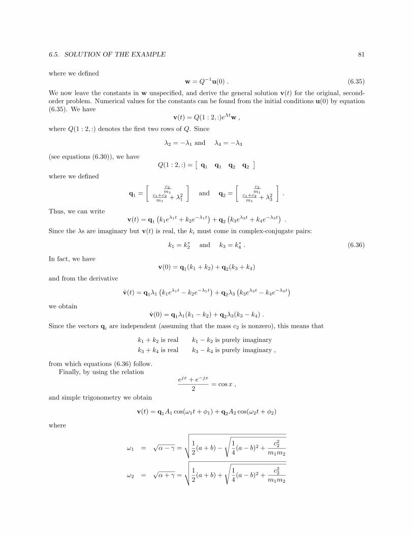
6.5. SOLUTION OF THE EXAMPLE 81
where we definedw = Q−1u(0) . (6.35)
We now leave the constants in w unspecified, and derive the general solution v(t) for the original, second-order problem. Numerical values for the constants can be found from the initial conditions u(0) by equation(6.35). We have
v(t) = Q(1 : 2, :)eΛtw ,
where Q(1 : 2, :) denotes the first two rows of Q. Since
λ2 = −λ1 and λ4 = −λ3
(see equations (6.30)), we haveQ(1 : 2, :) =
[q1 q1 q2 q2
]
where we defined
q1 =[ c2
m1c1+c2
m1+ λ2
1
]and q2 =
[ c2m1
c1+c2m1
+ λ23
].
Thus, we can writev(t) = q1
(k1e
λ1t + k2e−λ1t
)+ q2
(k3e
λ3t + k4e−λ3t
).
Since the λs are imaginary but v(t) is real, the ki must come in complex-conjugate pairs:
k1 = k∗2 and k3 = k∗4 . (6.36)
In fact, we havev(0) = q1(k1 + k2) + q2(k3 + k4)
and from the derivative
v(t) = q1λ1
(k1e
λ1t − k2e−λ1t
)+ q2λ3
(k3e
λ3t − k4e−λ3t
)
we obtainv(0) = q1λ1(k1 − k2) + q2λ3(k3 − k4) .
Since the vectors qi are independent (assuming that the mass c2 is nonzero), this means that
k1 + k2 is real k1 − k2 is purely imaginaryk3 + k4 is real k3 − k4 is purely imaginary ,
from which equations (6.36) follow.Finally, by using the relation
ejx + e−jx
2= cos x ,
and simple trigonometry we obtain
v(t) = q1A1 cos(ω1t + φ1) + q2A2 cos(ω2t + φ2)
where
ω1 =√
α− γ =
√√√√12(a + b)−
√14(a− b)2 +
c22
m1m2
ω2 =√
α + γ =
√√√√12(a + b) +
√14(a− b)2 +
c22
m1m2

82 CHAPTER 6. ORDINARY DIFFERENTIAL SYSTEMS
and
a =c1 + c2
m1, b =
c2 + c3
m2.
Notice that these two frequencies depend only on the configuration of the system, and not on the initialconditions.
The amplitudes Ai and phases φi, on the other hand, depend on the constants ki as follows:
A1 = 2|k1| , A2 = 2|k3|φ1 = arctan2(Im(k1),Re(k1)) φ2 = arctan2(Im(k3), Re(k3))
where Re, Im denote the real and imaginary part and where the two-argument function arctan2 is defined asfollows for (x, y) 6= (0, 0)
arctan2(y, x) =
arctan( yx ) if x > 0
π + arctan( yx ) if x < 0
π2 if x = 0 and y > 0−π
2 if x = 0 and y < 0
and is undefined for (x, y) = (0, 0). This function returns the arctangent of y/x (notice the order of thearguments) in the proper quadrant, and extends the function by continuity along the y axis.
The two constants k1 and k3 can be found from the given initial conditions v(0) and v(0) from equations(6.35) and (6.25).

CS 296.4
Mathematical Modelling of Continuous Systems
Carlo TomasiDuke University
Fall 2002

Chapter 7
Stochastic State Estimation
Perhaps the most important part of studying a problem in robotics or vision, as well as in most othersciences, is to determine a good model for the phenomena and events that are involved. For instance,studying manipulation requires defining models for how a robot arm can move and for how it interactswith the world. Analyzing image motion implies defining models for how points move in space and howthis motion projects onto the image. When motion is involved, as is very often the case, models take onfrequently the form of dynamic systems. A dynamic system is a mathematical description of a quantity thatevolves over time. The theory of dynamic systems is both rich and fascinating. Although in this chapterwe will barely scratch its surface, we will consider one of its most popular and useful aspects, the theoryof state estimation, in the particular form of Kalman filtering. To this purpose, an informal definition of adynamic system is given in the next section. The definition is then illustrated by setting up the dynamicsystem equations for a simple but realistic application, that of modeling the trajectory of an enemy mortarshell. In sections 7.3 through 7.5, we will develop the theory of the Kalman filter, and in section 7.6 wewill see that the shell can be shot down before it hits us. As discussed in section 7.7, Kalman filtering hasintimate connections with the theory of algebraic linear systems we have developed in chapters 2 and 3.
7.1 Dynamic Systems
In its most general meaning, the term system refers to some physical entity on which some action is performedby means of an input u. The system reacts to this input and produces an output y (see figure 7.1).
A dynamic system is a system whose phenomena occur over time. One often says that a system evolvesover time. Simple examples of a dynamic system are the following:
• An electric circuit, whose input is the current in a given branch and whose output is a voltage acrossa pair of nodes.
• A chemical reactor, whose inputs are the external temperature, the temperature of the gas beingsupplied, and the supply rate of the gas. The output can be the temperature of the reaction product.
input outputsystem
Su y
Figure 7.1: A general system.
83

84 CHAPTER 7. STOCHASTIC STATE ESTIMATION
• A mass suspended from a spring. The input is the force applied to the mass and the output is theposition of the mass.
In all these examples, what is input and what is output is a choice that depends on the application. Also,all the quantities in the examples vary continuously with time. In other cases, as for instance for switchingnetworks and computers, it is more natural to consider time as a discrete variable. If time varies continuously,the system is said to be continuous; if time varies discretely, the system is said to be discrete.
7.1.1 State
Given a dynamic system, continuous or discrete, the modeling problem is to somehow correlate inputs(causes) with outputs (effects). The examples above suggest that the output at time t cannot be determinedin general by the value assumed by the input quantity at the same point in time. Rather, the output isthe result of the entire history of the system. An effort of abstraction is therefore required, which leads topostulating a new quantity, called the state, which summarizes information about the past and the presentof the system. Specifically, the value x(t) taken by the state at time t must be sufficient to determine theoutput at the same point in time. Also, knowledge of both x(t1) and u[t1,t2), that is, of the state at time t1and the input over the interval t1 ≤ t < t2, must allow computing the state (and hence the output) at timet2. For the mass attached to a spring, for instance, the state could be the position and velocity of the mass.In fact, the laws of classical mechanics allow computing the new position and velocity of the mass at timet2 given its position and velocity at time t1 and the forces applied over the interval [t1, t2). Furthermore,in this example, the output y of the system happens to coincide with one of the two state variables, and istherefore always deducible from the latter.
Thus, in a dynamic system the input affects the state, and the output is a function of the state. For adiscrete system, the way that the input changes the state at time instant number k into the new state attime instant k + 1 can be represented by a simple equation:
xk+1 = f(xk,uk, k)
where f is some function that represents the change, and uk is the input at time k. Similarly, the relationbetween state and output can be expressed by another function:
yk = h(xk, k) .
A discrete dynamic system is completely described by these two equations and an initial state x0. In general,all quantities are vectors.
For continuous systems, time does not come in quanta, so one cannot compute xk+1 as a function ofxk, uk, and k, but rather compute x(t2) as a functional φ of x(t1) and the entire input u over the interval[t1, t2):
x(t2) = φ(x(t1),u(·), t1, t2)where u(·) represents the entire function u, not just one of its values. A description of the system in termsof functions, rather than functionals, can be given in the case of a regular system, for which the functionalφ is continuous, differentiable, and with continuous first derivative. In that case, one can show that thereexists a function f such that the state x(t) of the system satisfies the differential equation
x(t) = f(x(t),u(t), t)
where the dot denotes differentiation with respect to time. The relation from state to output, on the otherhand, is essentially the same as for the discrete case:
y(t) = h(x(t), t) .
Specifying the initial state x0 completes the definition of a continuous dynamic system.

7.2. AN EXAMPLE: THE MORTAR SHELL 85
7.1.2 Uncertainty
The systems defined in the previous section are called deterministic, since the evolution is exactly determinedonce the initial state x at time 0 is known. Determinism implies that both the evolution function f and theoutput function h are known exactly. This is, however, an unrealistic state of affairs. In practice, the lawsthat govern a given physical system are known up to some uncertainty. In fact, the equations themselvesare simple abstractions of a complex reality. The coefficients that appear in the equations are known onlyapproximately, and can change over time as a result of temperature changes, component wear, and so forth.A more realistic model then allows for some inherent, unresolvable uncertainty in both f and h. Thisuncertainty can be represented as noise that perturbs the equations we have presented so far. A discretesystem then takes on the following form:
xk+1 = f(xk,uk, k) + ηk
yk = h(xk, k) + ξk
and for a continuous system
x(t) = f(x(t),u(t), t) + η(t)y(t) = h(x(t), t) + ξ(t) .
Without loss of generality, the noise distributions can be assumed to have zero mean, for otherwise the meancan be incorporated into the deterministic part, that is, in either f or h. The mean may not be known,but this is a different story: in general the parameters that enter into the definitions of f and h must beestimated by some method, and the mean perturbations are no different.
A common assumption, which is sometimes valid and always simplifies the mathematics, is that η and ξare zero-mean Gaussian random variables with known covariance matrices Q and R, respectively.
7.1.3 Linearity
The mathematics becomes particularly simple when both the evolution function f and the output functionh are linear. Then, the system equations become
xk+1 = Fkxk + Gkuk + ηk
yk = Hkxk + ξk
for the discrete case, and
x(t) = F (t)x(t) + G(t)u(t) + η(t)y(t) = H(t)x(t) + ξ(t)
for the continuous one. It is useful to specify the sizes of the matrices involved. We assume that the inputu is a vector in Rp, the state x is in Rn, and the output y is in Rm. Then, the state propagation matrix Fis n × n, the input matrix G is n × p, and the output matrix H is m × n. The covariance matrix Q of thesystem noise η is n× n, and the covariance matrix of the output noise ξ is m×m.
7.2 An Example: the Mortar Shell
In this section, the example of the mortar shell will be discussed in order to see some of the technical issuesinvolved in setting up the equations of a dynamic system. In particular, we consider discretization issuesbecause the physical system is itself continuous, but we choose to model it as a discrete system for easierimplementation on a computer.

86 CHAPTER 7. STOCHASTIC STATE ESTIMATION
In sections 7.3 through 7.5, we consider the state estimation problem: given observations of the outputy over an interval of time, we want to determine the state x of the system. This is a very important task.For instance, in the case of the mortar shell, the state is the (initially unknown) position and velocity of theshell, while the output is a set of observations made by a tracking system. Estimating the state then leads toenough knowledge about the shell to allow driving an antiaircraft gun to shoot the shell down in mid-flight.
You spotted an enemy mortar installation about thirty kilometers away, on a hill that looks about 0.5kilometers higher than your own position. You want to track incoming projectiles with a Kalman filter soyou can aim your guns accurately. You do not know the initial velocity of the projectiles, so you just guesssome values: 0.6 kilometers/second for the horizontal component, 0.1 kilometers/second for the verticalcomponent. Thus, your estimate of the initial state of the projectile is
x0 =
ddzz
=
−0.6300.10.5
where d is the horizontal coordinate, z is the vertical, you are at (0, 0), and dots denote derivatives withrespect to time.
From your high-school physics, you remember that the laws of motion for a ballistic trajectory are thefollowing:
d(t) = d(0) + d(0)t (7.1)
z(t) = z(0) + z(0)t− 12gt2 (7.2)
where g is the gravitational acceleration, equal to 9.8 × 10⁻³ kilometers per second squared. Since you donot trust your physics much, and you have little time to get ready, you decide to ignore air drag. Becauseof this, you introduce a state update covariance matrix Q = 0.1I4, where I4 is the 4× 4 identity matrix.
All you have to track the shells is a camera pointed at the mortar that will rotate so as to keep theprojectile at the center of the image, where you see a blob that increases in size as the projectile gets closer.Thus, the aiming angle of the camera gives you elevation information about the projectile’s position, and thesize of the blob tells you something about the distance, given that you know the actual size of the projectilesused and all the camera parameters. The projectile’s elevation is
e = 1000z
d(7.3)
when the projectile is at (d, z). Similarly, the size of the blob in pixels is
s =1000√d2 + z2
. (7.4)
You do not have very precise estimates of the noise that corrupts e and s, so you guess measurementcovariances Re = Rs = 1000, which you put along the diagonal of a 2× 2 diagonal measurement covariancematrix R.
7.2.1 The Dynamic System Equation
Equations (7.1) and (7.2) are continuous. Since you are taking measurements every dt = 0.2 seconds, youwant to discretize these equations. For the z component, equation (7.2) yields
z(t + dt)− z(t) = z(0) + z(0)(t + dt)− 12g(t + dt)2 −
[z(0) + z(0)t− 1
2gt2
]
= (z(0)− gt)dt− 12g(dt)2
= z(t)dt− 12g(dt)2 ,

7.2. AN EXAMPLE: THE MORTAR SHELL 87
since z(0)− gt = z(t).Consequently, if t + dt is time instant k + 1 and t is time instant k, you have
zk+1 = zk + zkdt− 12g(dt)2 . (7.5)
The reasoning for the horizontal component d is the same, except that there is no acceleration:
dk+1 = dk + dkdt . (7.6)
Equations (7.5) and (7.6) can be rewritten as a single system update equation
xk+1 = Fxk + Gu
where
xk =
dk
dk
zk
zk
is the state, the 4 × 4 matrix F depends on dt, the control scalar u is equal to −g, and the 4 × 1 controlmatrix G depends on dt. The two matrices F and G are as follows:
F =
1 0 0 0dt 1 0 00 0 1 00 0 dt 1
G =
00dt−dt2
2
.
7.2.2 The Measurement Equation
The two nonlinear equations (7.3) and (7.4) express the available measurements as a function of the truevalues of the projectile coordinates d and z. We want to replace these equations with linear approximations.To this end, we develop both equations as Taylor series around the current estimate and truncate them afterthe linear term. From the elevation equation (7.3), we have
ek = 1000zk
dk≈ 1000
[zk
dk
+zk − zk
dk
− zk
d2k
(dk − dk)
],
so that after simplifying we can redefine the measurement to be the discrepancy from the estimated value:
e′k = ek − 1000zk
dk
≈ 1000(zk
dk
− zk
d2k
dk) . (7.7)
We can proceed similarly for equation (7.4):
sk =1000√d2
k + z2k
≈ 1000√d2
k + z2k
− 1000dk
(d2k + z2
k)3/2(dk − dk)− 1000zk
(d2k + z2
k)3/2(zk − zk)
and after simplifying:
s′k = sk − 2000√d2 + z2
≈ −1000
[dk
(d2k + z2
k)3/2dk +
zk
(d2k + z2
k)3/2zk
]. (7.8)

88 CHAPTER 7. STOCHASTIC STATE ESTIMATION
The two measurements s′k and e′k just defined can be collected into a single measurement vector
yk =[
s′ke′k
],
and the two approximate measurement equations (7.7) and (7.8) can be written in the matrix form
yk = Hkxk (7.9)
where the measurement matrix Hk depends on the current state estimate xk:
Hk = −1000
0 dk
(d2k+z2
k)3/2 0 zk
(d2k+z2
k)3/2
0 zk
d2k
0 − 1dk
As the shell approaches us, we frantically start studying state estimation, and in particular Kalmanfiltering, in the hope to build a system that lets us shoot down the shell before it hits us. The next fewsections will be read under this impending threat.
Knowing the model for the mortar shell amounts to knowing the laws by which the object moves andthose that relate the position of the projectile to our observations. So what else is there left to do? From theobservations, we would like to know where the mortar shell is right now, and perhaps predict where it willbe in a few seconds, so we can direct an antiaircraft gun to shoot down the target. In other words, we wantto know xk, the state of the dynamic system. Clearly, knowing x0 instead is equivalent, at least when thedynamics of the system are known exactly (the system noise ηk is zero). In fact, from x0 we can simulatethe system up until time t, thereby determining xk as well. Most importantly, we do not want to have allthe observations before we shoot: we would be dead by then. A scheme that refines an initial estimation ofthe state as new observations are acquired is called a recursive1 state estimation system. The Kalman filteris one of the most versatile schemes for recursive state estimations. The original paper by Kalman (R. E.Kalman, “A new approach to linear filtering and prediction problems,” Transactions of the ASME JournalBasic Engineering, 82:34–45, 1960) is still one of the most readable treatments of this subject from the pointof view of stochastic estimation.
Even without noise, a single observation yk may not be sufficient to determine the state xk (in theexample, one observation happens to be sufficient). This is a very interesting aspect of state estimation. Itis really the ensemble of all observations that let one estimate the state, and yet observations are processedone at a time, as they become available. A classical example of this situation in computer vision is thereconstruction of three-dimensional shape from a sequence of images. A single image is two-dimensional, soby itself it conveys no three-dimensional information. Kalman filters exist that recover shape informationfrom a sequence of images. See for instance L. Matthies, T. Kanade, and R. Szeliski, “Kalman filter-based algorithms for estimating depth from image sequences,” International Journal of Computer Vision,3(3):209-236, September 1989; and T.J. Broida, S. Chandrashekhar, and R. Chellappa, “Recursive 3-Dmotion estimation from a monocular image sequence,” IEEE Transactions on Aerospace and ElectronicSystems, 26(4):639–656, July 1990.
Here, we introduce the Kalman filter from the simpler point of view of least squares estimation, sincewe have developed all the necessary tools in the first part of this course. The next section defines the stateestimation problem for a discrete dynamic system in more detail. Then, section 7.4 defines the essentialnotions of estimation theory that are necessary to understand the quantitative aspects of Kalman filtering.Section 7.5 develops the equation of the Kalman filter, and section 7.6 reconsiders the example of the mortarshell. Finally, section 7.7 establishes a connection between the Kalman filter and the solution of a linearsystem.
1The term “recursive” in the systems theory literature corresponds loosely to “incremental” or “iterative” in computerscience.

7.3. STATE ESTIMATION 89
7.3 State Estimation
In this section, the estimation problem is defined in some more detail. Given a discrete dynamic system
xk+1 = Fkxk + Gkuk + ηk (7.10)yk = Hkxk + ξk (7.11)
where the system noise ηk and the measurement noise ξk are Gaussian variables,
ηk ∼ N (0, Qk)ξk ∼ N (0, Rk) ,
as well as a (possibly completely wrong) estimate x0 of the initial state and an initial covariance matrix P0
of the estimate x0, the Kalman filter computes the optimal estimate xk|k at time k given the measurementsy0, . . . ,yk. The filter also computes an estimate Pk|k of the covariance of xk|k given those measurements.In these expressions, the hat means that the quantity is an estimate. Also, the first k in the subscript refersto which variable is being estimated, the second to which measurements are being used for the estimate.Thus, in general, xi|j is the estimate of the value that x assumes at time i given the first j +1 measurementsy0, . . . ,yj .
7.3.1 Update
The covariance matrix Pk|k must be computed in order to keep the Kalman filter running, in the followingsense. At time k, just before the new measurement yk comes in, we have an estimate xk|k−1 of the statevector xk based on the previous measurements y0, . . . ,yk−1. Now we face the problem of incorporatingthe new measurement yk into our estimate, that is, of transforming xk|k−1 into xk|k. If xk|k−1 were exact,we could compute the new measurement yk without even looking at it, through the measurement equation(7.11). Even if xk|k−1 is not exact, the estimate
yk|k−1 = Hkxk|k−1
is still our best bet. Now yk becomes available, and we can consider the residue
rk = yk − yk|k−1 = yk −Hkxk|k−1 .
If this residue is nonzero, we probably need to correct our estimate of the state xk, so that the new prediction
yk|k = Hkxk|k
of the measurement value is closer to the measurement yk than the old prediction
yk|k−1 = Hkxk|k−1
that we made just before the new measurement yk was available.The question however is, by how much should we correct our estimate of the state? We do not want to
make yk|k coincide with yk. That would mean that we trust the new measurement completely, but that we donot trust our state estimate xk|k−1 at all, even if the latter was obtained through a large number of previousmeasurements. Thus, we need some criterion for comparing the quality of the new measurement yk withthat of our old estimate xk|k−1 of the state. The uncertainty about the former is Rk, the covariance of theobservation error. The uncertainty about the state just before the new measurement yk becomes available isPk|k−1. The update stage of the Kalman filter uses Rk and Pk|k−1 to weigh past evidence (xk|k−1) and newobservations (yk). This stage is represented graphically in the middle of figure 7.2. At the same time, alsothe uncertainty measure Pk|k−1 must be updated, so that it becomes available for the next step. Because anew measurement has been read, this uncertainty becomes usually smaller: Pk|k < Pk|k−1.
The idea is that as time goes by the uncertainty on the state decreases, while that about the measurementsmay remain the same. Then, measurements count less and less as the estimate approaches its true value.

90 CHAPTER 7. STOCHASTIC STATE ESTIMATION
k | k-1y
Hk
xk | k-1^ xk | k
k | kP
x
Pk+1 | k
k+1 | k
propagatepropagatex
Pk-1 | k-1
k-1 | k-1
ykyk-1 yk+1
k
updatek | k-1P
k-1 k+1
time
Figure 7.2: The update stage of the Kalman filter changes the estimate of the current system state xk tomake the prediction of the measurement closer to the actual measurement yk. Propagation then accountsfor the evolution of the system state, as well as the consequent growing uncertainty.
7.3.2 Propagation
Just after arrival of the measurement yk, both state estimate and state covariance matrix have been updatedas described above. But between time k and time k + 1 both state and covariance may change. The statechanges according to the system equation (7.10), so our estimate xk+1|k of xk+1 given y0, . . . ,yk shouldreflect this change as well. Similarly, because of the system noise ηk, our uncertainty about this estimatemay be somewhat greater than one time epoch ago. The system equation (7.10) essentially “dead reckons”the new state from the old, and inaccuracies in our model of how this happens lead to greater uncertainty.This increase in uncertainty depends on the system noise covariance Qk. Thus, both state estimate andcovariance must be propagated to the new time k + 1 to yield the new state estimate xk+1|k and the newcovariance Pk+1|k. Both these changes are shown on the right in figure 7.2.
In summary, just as the state vector xk represents all the information necessary to describe the evolutionof a deterministic system, the covariance matrix Pk|k contains all the necessary information about theprobabilistic part of the system, that is, about how both the system noise ηk and the measurement noise ξk
corrupt the quality of the state estimate xk|k.Hopefully, this intuitive introduction to Kalman filtering gives you an idea of what the filter does, and
what information it needs to keep working. To turn these concepts into a quantitative algorithm we needsome preliminaries on optimal estimation, which are discussed in the next section. The Kalman filter itselfis derived in section 7.5.
7.4 BLUE Estimators
In what sense does the Kalman filter use covariance information to produce better estimates of the state?As we will se later, the Kalman filter computes the Best Linear Unbiased Estimate (BLUE) of the state. Inthis section, we see what this means, starting with the definition of a linear estimation problem, and thenconsidering the attributes “best” and “unbiased” in turn.
7.4.1 Linear Estimation
Given a quantity y (the observation) that is a known function of another (deterministic but unknown)quantity x (the state) plus some amount of noise,
y = h(x) + n , (7.12)

7.4. BLUE ESTIMATORS 91
the estimation problem amounts to finding a function
x = L(y)
such that x is as close as possible to x. The function L is called an estimator, and its value x given theobservations y is called an estimate. Inverting a function is an example of estimation. If the function h isinvertible and the noise term n is zero, then L is the inverse of h, no matter how the phrase “as close aspossible” is interpreted. In fact, in that case x is equal to x, and any distance between x and x must bezero. In particular, solving a square, nonsingular system
y = Hx (7.13)
is, in this somewhat trivial sense, a problem of estimation. The optimal estimator is then represented by thematrix
L = H−1
and the optimal estimate isx = Ly .
A less trivial example occurs, for a linear observation function, when the matrix H has more rows thancolumns, so that the system (7.13) is overconstrained. In this case, there is usually no inverse to H, andagain one must say in what sense x is required to be “as close as possible” to x. For linear systems, wehave so far considered the criterion that prefers a particular x if it makes the Euclidean norm of the vectory − Hx as small as possible. This is the (unweighted) least squares criterion. In section 7.4.2, we will seethat in a very precise sense ordinary least squares solve a particular type of estimation problem, namely, theestimation problem for the observation equation (7.12) with h a linear function and n Gaussian zero-meannoise with the indentity matrix for covariance.
An estimator is said to be linear if the function L is linear. Notice that the observation function h canstill be nonlinear. If L is required to be linear but h is not, we will probably have an estimator that producesa worse estimate than a nonlinear one. However, it still makes sense to look for the best possible linearestimator. The best estimator for a linear observation function happens to be a linear estimator.
7.4.2 Best
In order to define what is meant by a “best” estimator, one needs to define a measure of goodness of anestimate. In the least squares approach to solving a linear system like (7.13), this distance is defined as theEuclidean norm of the residue vector
y−Hx
between the left and the right-hand sides of equation (7.13), evaluated at the solution x. Replacing (7.13)by a “noisy equation”,
y = Hx + n (7.14)
does not change the nature of the problem. Even equation (7.13) has no exact solution when there are moreindependent equations than unknowns, so requiring equality is hopeless. What the least squares approachis really saying is that even at the solution x there is some residue
n = y−Hx (7.15)
and we would like to make that residue as small as possible in the sense of the Euclidean norm. Thus, anoverconstrained system of the form (7.13) and its “noisy” version (7.14) are really the same problem. Infact, (7.14) is the correct version, if the equality sign is to be taken literally.
The noise term, however, can be used to generalize the problem. In fact, the Euclidean norm of theresidue (7.15) treats all components (all equations in (7.14)) equally. In other words, each equation countsthe same when computing the norm of the residue. However, different equations can have noise terms of

92 CHAPTER 7. STOCHASTIC STATE ESTIMATION
different variance. This amounts to saying that we have reasons to prefer the quality of some equations overothers or, alternatively, that we want to enforce different equations to different degrees. From the pointof view of least squares, this can be enforced by some scaling of the entries of n or, even, by some lineartransformation of them:
n → Wn
so instead of minimizing ‖n‖2 = nT n (the square is of course irrelevant when it comes to minimization), wenow minimize
‖Wn‖2 = nT R−1n
whereR−1 = WT W
is a symmetric, nonnegative-definite matrix. This minimization problem, called weighted least squares, isonly slightly different from its unweighted version. In fact, we have
Wn = W (y−Hx) = Wy−WHx
so we are simply solving the systemWy = WHx
in the traditional, “unweighted” sense. We know the solution from normal equations:
x = ((WH)T WH)−1(WH)T Wy = (HT R−1H)−1HT R−1y .
Interestingly, this same solution is obtained from a completely different criterion of goodness of a solutionx. This criterion is a probabilistic one. We consider this different approach because it will let us show thatthe Kalman filter is optimal in a very useful sense.
The new criterion is the so-called minimum-covariance criterion. The estimate x of x is some functionof the measurements y, which in turn are corrupted by noise. Thus, x is a function of a random vector(noise), and is therefore a random vector itself. Intuitively, if we estimate the same quantity many times,from measurements corrupted by different noise samples from the same distribution, we obtain differentestimates. In this sense, the estimates are random.
It makes therefore sense to measure the quality of an estimator by requiring that its variance be as smallas possible: the fluctuations of the estimate x with respect to the true (unknown) value x from one estimationexperiment to the next should be as small as possible. Formally, we want to choose a linear estimator Lsuch that the estimates x = Ly it produces minimize the following covariance matrix:
P = E[(x− x)(x− x)T ] .
Minimizing a matrix, however, requires a notion of “size” for matrices: how large is P? Fortunately, mostinteresting matrix norms are equivalent, in the sense that given two different definitions ‖P‖1 and ‖P‖2 ofmatrix norm there exist two positive scalars α, β such that
α‖P‖1 < ‖P‖2 < β‖P‖1 .
Thus, we can pick any norm we like. In fact, in the derivations that follow, we only use properties shared byall norms, so which norm we actually use is irrelevant. Some matrix norms were mentioned in section 3.2.
7.4.3 Unbiased
In additionto requiring our estimator to be linear and with minimum covariance, we also want it to beunbiased, in the sense that if repeat the same estimation experiment many times we neither consistentlyoverestimate nor consistently underestimate x. Mathematically, this translates into the following require-ment:
E[x− x] = 0 and E[x] = E[x] .

7.4. BLUE ESTIMATORS 93
7.4.4 The BLUE
We now address the problem of finding the Best Linear Unbiased Estimator (BLUE)
x = Ly
of x given that y depends on x according to the model (7.14), which is repeated here for convenience:
y = Hx + n . (7.16)
First, we give a necessary and sufficient condition for L to be unbiased.
Lemma 7.4.1 Let n in equation (7.16) be zero mean. Then the linear estimator L is unbiased if an only if
LH = I ,
the identity matrix.
Proof.
E[x− x] = E[x− Ly] = E[x− L(Hx + n)]= E[(I − LH)x]− E[Ln] = (I −HL)E[x]
since E[Ln] = LE[n] and E[n] = 0. For this to hold for all x we need I − LH = 0. ∆
And now the main result.
Theorem 7.4.2 The Best Linear Unbiased Estimator (BLUE)
x = Ly
for the measurement modely = Hx + n
where the noise vector n has zero mean and covariance R is given by
L = (HT R−1H)−1HT R−1
and the covariance of the estimate x is
P = E[(x− x)(x− x)T ] = (HT R−1H)−1 . (7.17)
Proof. We can write
P = E[(x− x)(x− x)T ] = E[(x− Ly)(x− Ly)T ]= E[(x− LHx− Ln)(x− LHx− Ln)T ] = E[((I − LH)x− Ln)((I − LH)x− Ln)T ]= E[LnnT LT ] = LE[nnT ] LT = LRLT
because L is unbiased, so that LH = I.To show that
L0 = (HT R−1H)−1HT R−1 (7.18)
is the best choice, let L be any (other) linear unbiased estimator. We can trivially write
L = L0 + (L− L0)

94 CHAPTER 7. STOCHASTIC STATE ESTIMATION
and
P = LRLT = [L0 + (L− L0)]R[L0 + (L− L0)]T
= L0RLT0 + (L− L0)RLT
0 + L0R(L− L0)T + (L− L0)R(L− L0)T .
From (7.18) we obtain
RLT0 = RR−1H(HT R−1H)−1 = H(HT R−1H)−1
so that(L− L0)RLT
0 = (L− L0)H(HT R−1H)−1 = (LH − L0H)(HT R−1H)−1 .
But L and L0 are unbiased, so LH = L0H = I, and
(L− L0)RLT0 = 0 .
The term L0R(L− L0)T is the transpose of this, so it is zero as well. In conclusion,
P = L0RLT0 + (L− L0)R(L− L0)T ,
the sum of two positive definite or at least semidefinite matrices. For such matrices, the norm of the sumis greater or equal to either norm, so this expression is minimized when the second term vanishes, that is,when L = L0.
This proves that the estimator given by (7.18) is the best, that is, that it has minimum covariance. Toprove that the covariance P of x is given by equation (7.17), we simply substitute L0 for L in P = LRLT :
P = L0RLT0 = (HT R−1H)−1HT R−1RR−1H(HT R−1H)−1
= (HT R−1H)−1HT R−1H(HT R−1H)−1 = (HT R−1H)−1
as promised. ∆
7.5 The Kalman Filter: Derivation
We now have all the components necessary to write the equations for the Kalman filter. To summarize,given a linear measurement equation
y = Hx + n
where n is a Gaussian random vector with zero mean and covariance matrix R,
n ∼ N (0, R) ,
the best linear unbiased estimate x of x is
x = PHT R−1y
where the matrixP
∆= E[(x− x)(x− x)T ] = (HT R−1H)−1
is the covariance of the estimation error.Given a dynamic system with system and measurement equations
xk+1 = Fkxk + Gkuk + ηk (7.19)yk = Hkxk + ξk

7.5. THE KALMAN FILTER: DERIVATION 95
where the system noise ηk and the measurement noise ξk are Gaussian random vectors,
ηk ∼ N (0, Qk)ξk ∼ N (0, Rk) ,
as well as the best, linear, unbiased estimate x0 of the initial state with an error covariance matrix P0, theKalman filter computes the best, linear, unbiased estimate xk|k at time k given the measurements y0, . . . ,yk.The filter also computes the covariance Pk|k of the error xk|k − xk given those measurements. Computationoccurs according to the phases of update and propagation illustrated in figure 7.2. We now apply the resultsfrom optimal estimation to the problem of updating and propagating the state estimates and their errorcovariances.
7.5.1 Update
At time k, two pieces of data are available. One is the estimate xk|k−1 of the state xk given measurementsup to but not including yk. This estimate comes with its covariance matrix Pk|k−1. Another way of sayingthis is that the estimate xk|k−1 differs from the true state xk by an error term ek whose covariance is Pk|k−1:
xk|k−1 = xk + ek (7.20)
withE[ekeT
k ] = Pk|k−1 .
The other piece of data is the new measurement yk itself, which is related to the state xk by the equation
yk = Hkxk + ξk (7.21)
with error covarianceE[ξkξT
k ] = Rk .
We can summarize this available information by grouping equations 7.20 and 7.21 into one, and packagingthe error covariances into a single, block-diagonal matrix. Thus, we have
y = Hxk + n
where
y =[
xk|k−1
yk
], H =
[I
Hk
], n =
[ek
ξk
],
and where n has covariance
R =[
Pk|k−1 00 Rk
].
As we know, the solution to this classical estimation problem is
xk|k = Pk|kHT R−1y
Pk|k = (HT R−1H)−1 .
This pair of equations represents the update stage of the Kalman filter. These expressions are somewhatwasteful, because the matrices H and R contain many zeros. For this reason, these two update equationsare now rewritten in a more efficient and more familiar form. We have
P−1k|k = HT R−1H
=[
I HTk
] [P−1
k|k−1 00 R−1
k
] [I
Hk
]
= P−1k|k−1 + HT
k R−1k Hk

96 CHAPTER 7. STOCHASTIC STATE ESTIMATION
and
xk|k = Pk|kHT R−1y
= Pk|k[
P−1k|k−1 HT
k R−1k
] [xk|k−1
yk
]
= Pk|k(P−1k|k−1xk|k−1 + HT
k R−1k yk)
= Pk|k((P−1k|k −HT
k R−1k Hk)xk|k−1 + HT
k R−1k yk)
= xk|k−1 + Pk|kHTk R−1
k (yk −Hkxk|k−1) .
In the last line, the differencerk
∆= yk −Hkxk|k−1
is the residue between the actual measurement yk and its best estimate based on xk|k−1, and the matrix
Kk∆= Pk|kHT
k R−1k
is usually referred to as the Kalman gain matrix, because it specifies the amount by which the residue mustbe multiplied (or amplified) to obtain the correction term that transforms the old estimate xk|k−1 of thestate xk into its new estimate xk|k.
7.5.2 Propagation
Propagation is even simpler. Since the new state is related to the old through the system equation 7.19, andthe noise term ηk is zero mean, unbiasedness requires
xk+1|k = Fkxk|k + Gkuk ,
which is the state estimate propagation equation of the Kalman filter. The error covariance matrix is easilypropagated thanks to the linearity of the expectation operator:
Pk+1|k = E[(xk+1|k − xk+1)(xk+1|k − xk+1)T ]
= E[(Fk(xk|k − xk)− ηk)(Fk(xk|k − xk)− ηk)T ]
= FkE[(xk|k − xk)(xk|k − xk)T ]FTk + E[ηkηT
k ]
= FkPk|kFTk + Qk
where the system noise ηk and the previous estimation error xk|k − xk were assumed to be uncorrelated.
7.5.3 Kalman Filter Equations
In summary, the Kalman filter evolves an initial estimate and an initial error covariance matrix,
x0|−1∆= x0 and P0|−1
∆= P0 ,
both assumed to be given, by the update equations
xk|k = xk|k−1 + Kk(yk −Hkxk|k−1)
P−1k|k = P−1
k|k−1 + HTk R−1
k Hk
where the Kalman gain is defined asKk = Pk|kHT
k R−1k
and by the propagation equations
xk+1|k = Fkxk|k + Gkuk
Pk+1|k = FkPk|kFTk + Qk .

7.6. RESULTS OF THE MORTAR SHELL EXPERIMENT 97
5 10 15 20 25 30 35−0.2
0
0.2
0.4
0.6
0.8
1
1.2
1.4true (dashed) and estimated (solid) missile trajectory
Figure 7.3: The true and estimated trajectories get closer to one another. Trajectories start on the right.
7.6 Results of the Mortar Shell Experiment
In section 7.2, the dynamic system equations for a mortar shell were set up. Matlab routines available throughthe class Web page implement a Kalman filter (with naive numerics) to estimate the state of that systemfrom simulated observations. Figure 7.3 shows the true and estimated trajectories. Notice that coincidenceof the trajectories does not imply that the state estimate is up-to-date. For this it is also necessary that anygiven point of the trajectory is reached by the estimate at the same time instant. Figure 7.4 shows that thedistance between estimated and true target position does indeed converge to zero, and this occurs in timefor the shell to be shot down. Figure 7.5 shows the 2-norm of the covariance matrix over time. Notice thatthe covariance goes to zero only asymptotically.
7.7 Linear Systems and the Kalman Filter
In order to connect the theory of state estimation with what we have learned so far about linear systems,we now show that estimating the initial state x0 from the first k + 1 measurements, that is, obtaining x0|k,amounts to solving a linear system of equations with suitable weights for its rows.
The basic recurrence equations (7.10) and (7.11) can be expanded as follows:
yk = Hkxk + ξk = Hk(Fk−1xk−1 + Gk−1uk−1 + ηk−1) + ξk
= HkFk−1xk−1 + HkGk−1uk−1 + Hkηk−1 + ξk
= HkFk−1(Fk−2xk−2 + Gk−2uk−2 + ηk−2) + HkGk−1uk−1 + Hkηk−1 + ξk
= HkFk−1Fk−2xk−2 + Hk(Fk−1Gk−2uk−2 + Gk−1uk−1) +Hk(Fk−1ηk−2 + ηk−1) + ξk
...= HkFk−1 . . . F0x0 + Hk(Fk−1 . . . F1G0u0 + . . . + Gk−1uk−1) +
Hk(Fk−1 . . . F1η0 + . . . + ηk−1) + ξk

98 CHAPTER 7. STOCHASTIC STATE ESTIMATION
0 5 10 15 20 25 300
0.2
0.4
0.6
0.8
1
1.2
1.4
1.6
1.8
2distance between true and estimated missile position vs. time
Figure 7.4: The estimate actually closes in towards the target.
0 5 10 15 20 25 300
5
10
15
20
25
30
35
40norm of the state covariance matrix vs time
Figure 7.5: After an initial increase in uncertainty, the norm of the state covariance matrix converges tozero. Upwards segments correspond to state propagation, downwards ones to state update.

7.7. LINEAR SYSTEMS AND THE KALMAN FILTER 99
or in a more compact form,
yk = HkΦ(k − 1, 0)x0 + Hk
k∑
j=1
Φ(k − 1, j)Gj−1uj−1 + νk (7.22)
where
Φ(l, j) ={
Fl . . . Fj for l ≥ j1 for l < j
and the term
νk = Hk
k∑
j=1
Φ(k − 1, j)ηj−1 + ξk
is noise.The key thing to notice about this somewhat intimidating expression is that for any k it is a linear system
in x0, the initial state of the system. We can write one system like the one in equation (7.22) for every valueof k = 0, . . . , K, where K is the last time instant considered, and we obtain a large system of the form
zK = ΨKx0 + gK + nK (7.23)
where
zK =
y0...
yK
ΨK =
H0
H1F0
...HKΦ(K − 1, 0)
gK =
0H1G0u0
...HK(Φ(K − 1, 1)G0u0 + . . . + Φ(K − 1,K)GK−1uK−1)
nK =
ν0
...νK
.
Without knowing anything about the statistics of the noise vector nK in equation (7.23), the best wecan do is to solve the system
zK = ΨKx0 + gK
in the sense of least squares, to obtain an estimate of x0 from the measurements y0, . . . ,yK :
x0|K = Ψ†K(zK − gK)
where Ψ†K is the pseudoinverse of ΨK . We know that if ΨK has full rank, the result with the pseudoinverseis the same as we would obtain by solving the normal equations, so that
Ψ†K = (ΨTKΨK)−1ΨT
K .
The least square solution to system (7.23) minimizes the residue between the left and the right-hand sideunder the assumption that all equations are to be treated the same way. This is equivalent to assuming

100 CHAPTER 7. STOCHASTIC STATE ESTIMATION
that all the noise terms in nK are equally important. However, we know the covariance matrices of all thesenoise terms, so we ought to be able to do better, and weigh each equation to keep these covariances intoaccount. Intuitively, a small covariance means that we believe in that measurement, and therefore in thatequation, which should consequently be weighed more heavily than others. The quantitative embodiment ofthis intuitive idea is at the core of the Kalman filter.
In summary, the Kalman filter for a linear system has been shown to be equivalent to a linear equationsolver, under the assumption that the noise that affects each of the equations has the same probabilitydistribution, that is, that all the noise terms in nK in equation 7.23 are equally important. However, theKalman filter differs from a linear solver in the following important respects:
1. The noise terms in nK in equation 7.23 are not equally important. Measurements come with covariancematrices, and the Kalman filter makes optimal use of this information for a proper weighting of eachof the scalar equations in (7.23). Better information ought to yield more accurate results, and this isin fact the case.
2. The system (7.23) is not solved all at once. Rather, an initial solution is refined over time as newmeasurements become available. The final solution can be proven to be exactly equal to solvingsystem (7.23) all at once. However, having better and better approximations to the solution as newdata come in is much preferable in a dynamic setting, where one cannot in general wait for all the datato be collected. In some applications, data my never stop arriving.
3. A solution for the estimate xk|k of the current state is given, and not only for the estimate x0|k of theinitial state. As time goes by, knowledge of the initial state may obsolesce and become less and lessuseful. The Kalman filter computes up-to-date information about the current state.