Gauging spatial symmetries and the classification of topological crystalline phases

Ryan Thorngren1, 2 and Dominic V. Else3

1Department of Mathematics, University of California, Berkeley, CA 94720, USA2Kavli Institute for Theoretical Physics, University of California, Santa Barbara, CA 93106, USA

3Department of Physics, University of California, Santa Barbara, CA 93106, USA

We put the theory of interacting topological crystalline phases on a systematic footing. These aretopological phases protected by space-group symmetries. Our central tool is an elucidation of whatit means to “gauge” such symmetries. We introduce the notion of a crystalline topological liquid,and argue that most (and perhaps all) phases of interest are likely to satisfy this criterion. We provea Crystalline Equivalence Principle, which states that in Euclidean space, crystalline topologicalliquids with symmetry group G are in one-to-one correspondence with topological phases protectedby the same symmetry G, but acting internally, where if an element of G is orientation-reversing,it is realized as an anti-unitary symmetry in the internal symmetry group. As an example, weexplicitly compute, using group cohomology, a partial classification of bosonic symmetry-protectedtopological (SPT) phases protected by crystalline symmetries in (3+1)-D for 227 of the 230 spacegroups. For the 65 space groups not containing orientation-reversing elements (Sohncke groups),there are no cobordism invariants which may contribute phases beyond group cohomology, and sowe conjecture our classification is complete.

Symmetry is an important feature of many physicalsystems. Many phases of matter can be characterized inpart by the way the symmetry is implemented. For exam-ple, liquids and solids are distinguished by whether or notthey spontaneously break spatial symmetries. In fact, itwas once thought that all known phases could be dis-tinguished by their symmetries and that all continuousphase transitions were spontaneous symmetry breakingtransitions. The discovery of topological order [1] showedthat, at zero temperature, there are quantum phases ofmatter that can be distinguished by patterns of long-range entanglement without the need to invoke symme-try. However, even for topological phases symmetry isimportant. Any symmetry that is not spontaneouslybroken in a topological phase must have some action onthe topological structure of the phase, and different suchpatterns can distinguish different phases. Even a phaseof matter that is trivial without symmetry can becomenon-trivial when considering how symmetry is imple-mented. Topological phases distinguished by symmetryare known as symmetry-enriched topological (SET)[2–8]or symmetry-protected topological (SPT)[9–26] dependingon whether they are nontrivial or trivial without symme-try, respectively.

For internal symmetries, which do not move pointsin space around, very general and powerful ways ofunderstanding SPT and SET phases have been formu-lated in terms of mathematical notions such as groupcohomology[17], category theory[7], and cobordisms[21,27]. On the other hand, such techniques have not, so far,been extended to the case of space group symmetries. Werefer to these topological phases enriched by space-groupsymmetries as topological crystalline phases. This is asignificant omission because any system which arrangesitself into a regular crystal lattice is invariant underone of 230 space groups in three dimensions. Fermionicphases of matter protected by space-group symmetriesare called topological crystalline insulators or topological

crystalline superconductors depending on whether chargeis conserved [28–33]. Progress towards a general classi-fication in free-fermion systems has been made [34–40]and some understanding of the effect of interactions beenachieved [41–45]. Meanwhile, intrinsically strongly inter-acting phases protected by spatial symmetries have alsobeen found [3, 7, 46–54]. In particular Ref. [55] gave anapproach for deriving the general classification of inter-acting SPT phases protected by a group of spatial sym-metries that leave a given point invariant. However, forSETs and/or general space groups, there is so far no sys-tematic theory analogous to the one that exists for inter-nal symmetries, except in one dimension [56]. Our goalin this paper is to fill this gap.

We will adopt two complementary and related view-points to the classification. The first viewpoint is in termsof topological quantum field theories (TQFTs), which arebelieved to describe the low-energy physics of topologi-cal phases. We state and motivate a proposal for how toimplement a spatial symmetry in a TQFT.

Our second, more concrete, viewpoint is based on theidea of understanding the SPT or SET order of a systemby studying its response to a gauge field. For example,SPTs in (2+1)-D protected by an internal U(1) symme-try can be identified by the topological response to a U(1)gauge field. All such possible responses are described bythe Chern-Simons action

S =k

4π

∫A ∧ dA. (0.1)

The coefficient k has a physical interpretation as thequantized Hall conductance. Because it is quantized, theonly way to get between systems with different values of kis if U(1) symmetry is broken or the gap closes. Further,since this is the only term that may appear, we learn thatthe different U(1) SPTs in 2+1D are labelled by this in-teger. We call this procedure of coupling a G-symmetricsystem to a background G gauge field “gauging” the G

arX

iv:1

612.

0084

6v6

[co

nd-m

at.s

tr-e

l] 1

2 Se

p 20

17

2

symmetry, though strictly speaking we do not considermaking the gauge field dynamical. Stricter terminologywould call the dynamical gauge theory the result of gaug-ing and our procedure the first step, called equivarianti-zation, a mouthful, or pregauging. Many of the generalapproaches to SPT and SET phases can be formulatedin terms of gauging[6, 7, 57, 58].

We want to apply similar approaches to the study ofsystems with spatial symmetry. So we will ask the ques-tion

Question 1. What does it mean to gauge a spatial sym-metry?

We will give what we believe to be the definitive answerto this question, motivated by the intuition of “gaugefluxes” which for spatial symmetries are crystallographicdefects such as dislocations and disclinations. Thereseems to be a natural generalization of this to symmetrieswhich act on spacetime as well, such as time reversal sym-metry or time translation. We will mention briefly thisgeneralization and how the classification extends to thesespacetime symmetries, where it agrees with known groupcohomology classifications of time reversal-invariant andFloquet SPTs, respectively.

Using the two viewpoints mentioned above, we willelucidate the general theory of crystalline topologicalphases. Our results are based on a key physical assump-tion, namely that the phases of matter under consid-eration are crystalline topological liquid, which roughlymeans that, although crystalline, they preserve a cer-tain degree of “fluidity” in the low-energy limit. Theidea is motivated by the notion of “topological liquids”which have an IR limit that is described by a topolog-ical quantum field theory (TQFT), i.e. the long-rangephysics is only sensitive to the topology of the back-ground manifold. This is in contrast to “fracton” topo-logical phases[59–62] where no such topological IR limitexists1. Crystalline topological liquids are a generaliza-tion of topological liquids to systems with crystal sym-metries.

The main result of this paper is the following.

Crystalline Equivalence Principle: The clas-sification of crystalline topological liquids with spa-tial symmetry group G is the same as the classifi-cation of topological phases with internal symmetryG.

Compare Ref. 63, where a similar principle was con-jectured for symmetry groups containing time translationsymmetry. This result holds for systems living on a con-tractible space, ie. Euclidean space in d dimensions. Onother manifolds, for example Euclidean space with some

1 Although see Section VII.

Number Name Classification1 p1 02 p2 Z×4

2

3 pm Z×22

4 pg 05 cm Z2

6 p2mm Z×82

7 p2mg Z×32

8 p2gg Z×22

9 c2mm Z×52

10 p4 Z2 × Z×24

11 p4mm Z×62

12 p4gm Z×22 × Z4

13 p3 Z×33

14 p3m1 Z2

15 p31m Z2 × Z3

16 p6 Z×22 × Z×2

3

17 p6mm Z×42

TABLE I. The classification of bosonic SPT phases in (2+1)-D protected by space group symmetries, for each of the 172-D space groups (sometimes known as “wallpaper groups”).

holes, some new things happen. We note for this corre-spondence, orientation-reversing symmetries in the spacegroup must correspond to anti-unitary symmetries in theinternal group.

We emphasize that the Crystalline Equivalence Prin-ciple is expected to hold for both bosonic and fermionic2

systems, and for both SPT and SET phases. As an ex-ample of results that one can deduce from this generalprinciple, we find that bosonic SPT phases protected byorientation-preserving unitary spatial symmetry G areclassified by the group cohomology Hd+1(G,U(1)), sincethat is the classification of internal SPTs with symmetryG (See Appendix A for more details on the definition ofH.) This agrees with a recent classification of a class oftensor networks with spatial symmetries[54]. In (3+1)-D,for space groups containing orientation-reversing trans-formations, this classification is expected to be incom-plete, just as it is for internal symmetry groups contain-ing anti-unitary symmetries[21]. Applying the principleto fermionic systems, one obtains a partial classificationof fermionic SPT’s protected by space-group symmetriesfrom “group supercohomology” [22] and a complete clas-sification of fermionic crystalline SPT’s from cobordismtheory [27], with some caveats. We attempt this in sec-tion VII B for crystalline topological superconductors andinsulators.

Our results allow for the classification to be explicitlycomputed in many cases. For example, Table I shows theclassification of bosonic SPT phases protected by space-group symmetry in (2+1)-D as obtained from group co-

2 There are some caveats for fermionic systems: systems with R2 =+1, where R is a reflection, are in correspondence with systemswith T 2 = (−1)F , where T is time-reversal, and vice versa.

3

homology. For more details of how Table I was computed,and the (3+1)-D version of the table, see Appendix B.

The outline of our paper is as follows. In Section I, weintroduce the notion of a crystalline topological liquid.Then, in Section II we introduce the key ideas involved ingauging a spatial symmetry. Specifically, in section II Awe discuss our definition of crystalline gauge field. Thenin II B we argue that crystalline topological liquids nat-urally couple to such crystalline gauge fields. In II C weuse the gauging picture to derive the Crystalline Equiv-alence Principle, which applies to the physically relevantcase of phases of matter in contractible space Rd. In II Dwe discuss extensions to non-contractible spaces and ageneral classification result for crystalline gauge fields.

In Section III we give a construction of many crys-talline topological liquids from ordinary topological liq-uids by considering systems which carry both a spatialG symmetry and an internal G symmetry.

In Section IV we describe our approach towards classi-fying crystalline topological liquids using topological re-sponse. In IV A, this is defined in terms of fusion andbraiding of symmetry fluxes. In IV B it is described interms of effective topological actions. Finally, in IV C,we give many examples of crystalline gauge backgroundsand compute the resulting partition functions in exactlysolvable models. This section is particularly important,as it elucidates where some of the familiar features ofordinary SPT phases appear in crystalline SPT phases.

In Section V, we describe how our methods canbe placed into a general context of position-dependenttopological limit, and discuss implications of emergentLorentz invariance or lack thereof.

In Section VI, we derive several general structural re-sults about the classification of crystalline SPTs (invert-ible crystalline topological liquids).

We give generalizations of our methods in SectionVII, including Floquet phases in VII A and phases be-yond ordinary equivariant cohomology in VII B includingfermions. In VII C we discuss how our methods apply totopological terms of sigma models.

In Section VIII, we describe some ways in which ourcrystalline topological liquid assumption can fail and in-clude some comments about fracton phases.

In Section IX we discuss questions for future work.We hope this paper will inspire the discovery of many

curious quantum crystals.

I. THE TOPOLOGICAL LIMIT OF ACRYSTALLINE TOPOLOGICAL PHASE

In this section, we will briefly outline the argumentsbased on topological quantum field theory (TQFT) whichlead to the Crystalline Equivalence Principle. The math-ematical details are left to Section V. The underlyingphysical concept is that of a smooth state. A smoothstate is a ground state of a lattice Hamiltonian that isdefined on a lattice which is much finer than the unit

cell with respect to the translation symmetry, such thatthe lattice spacing l and the correlation length ξ are muchsmaller than the minimum radius R of spatial variationwithin the unit cell. The condition ξ, l a (where a isthe unit cell size) was discussed as an assumption for clas-sifying crystalline phases in Ref. [64]; our “smooth state”assumption is slightly stronger since we require ξ, l R.This implies the condition of Ref. [64] since R < a, butthe converse need not be true if there are regions in theunit cell where spatial variation happens rapidly (so thatR a).

A smooth state might not seem like the kind of systemone would normally consider; a physical example wouldbe a graphene heterostructure in which a lattice mis-match between two layers results in a Moire pattern withvery large unit cell [65]. Nevertheless, it is reasonable toexpect that the classification of smooth states would bethe same as the classification of states in general. Wewill leave a rigorous proof for future work; presently, wemerely state it as a conjecture and examine the conse-quences.

A very important property of a smooth state is that itcan be coarse-grained while preserving the spatial sym-metries. This is allowed only so long as the coarse-grainedlattice is still small compared to the unit cell size, butgiven the assumption ξ a this still allows us to reacha “topological limit”, by which we mean that ξ becomesmuch smaller than the coarse-grained lattice spacing. Im-portantly, since the RG can take place in the neighbor-hood of any given point in the unit cell, the effective fieldtheory that we obtain in this topological limit will stillbe spatially-dependent. (For this reason, we will avoidreferring to the topological limit as an “IR limit”, whichwould be misleading since the unit cell size – but not thelattice spacing! – is still an important length scale).

We expect that this topological limit will, as in thecase of systems without spatial symmetries, be describedby a topological quantum field theory (TQFT). In fact,given the afore-mentioned spatial dependence, it shouldbe described by a spatially-dependent TQFT. We give theprecise mathematical definition of this concept in SectionV.

Hence, we can define

Definition 1. A crystalline topological liquid is a phaseof matter that is characterized by a spatially-dependentTQFT acted upon by spatial symmetries.

We expect that this class of systems is quite large. Cer-tainly, it includes ordinary topological liquids (which, bydefinition, have no explicit spatial symmetries and can becharacterized by a spatially-constant TQFT). Moreover,spatially-dependent TQFTs can capture a wide range ofother topological crystalline phenomena, as we shall see.

In Section V, we sketch a proof that on contractiblespaces, spatially-dependent TQFTs with spatial symme-tries are in one to one correspondence with spatially con-stant TQFTs with internal symmetries. Since the latterare expected to characterize topological phases with in-

4

(a) Smooth state (b) Topological limit

FIG. 1. (a) In a smooth state, the lattice spacing and the correlation length ξ are much less than the unit cell size a and theradius of spatial variation. (b) The topological response of a crystalline topological liquid is captured by a spatially-dependentTQFT that captures the spatial dependence within each unit cell but “forgets” about the lattice.

ternal symmetries, the Crystalline Equivalence Principlefollows. In the following sections, we we will discuss howto understand this result in more concrete ways withoutresorting to the highly abstract formalism of TQFTs.

II. CRYSTALLINE GAUGE FIELDS

A. Gauge fluxes and crystal defects

In order to understand crystalline topological phases,we want to study what it might mean to couple to abackground gauge field for a symmetry group G involv-ing some transformation of space itself. More generally,we believe a framework exists where one can also con-sider symmetries that transform space-time. However,for simplicity and to maintain contact with Hamiltonianmodels we will focus on purely spatial symmetries. Wecall our object of study the crystalline gauge field.

A special case of a background gauge field is an isolatedgauge flux. Isolated gauge fluxes are familiar objects forinternal symmetries. They are objects in space of codi-mension 2 (i.e. points in 2-D, curves in 3-D) which arelabelled by a group element g ∈ G, and a particle mov-ing all the way around one is acted upon by g. Actually,for a non-Abelian group only the conjugacy class of g isgauge-invariant.

Gauge fluxes for spatial symmetries are also labelledby conjugacy classes of G. They are also well-known,but not under that name; they are more commonly re-ferred to as crystal defects. For example, a gauge fluxfor translational symmetry is a dislocation and a gaugeflux for a rotational symmetry is a disclination (Fig 2).In 3d, the direction of dislocation does not have to bein the plane perpendicular to the defect, as in a screwdislocation. A defect for reflection symmetry is like theMobius band (a cross cap). For a glide reflection we alsoinsert a shift in the lattice as we go around the band. Wewill see how this zoo of defect configurations is tamed bytopology.

Generalizing these examples, we can give a systematicdefinition of crystalline gauge flux, and more generally ofa crystalline gauge field. For motivation, one can lookagain at Fig 2. The original lattice Λ is a regular squareor kagome lattice. The crucial property the defect latticeΣ is that away from the singular point in the middle,it looks locally the same as Λ, meaning that in a neigh-borhood of every face except the central one there is aninvertible map sending Σ to Λ. However, there is noglobal map sending Σ to Λ. Indeed, if we try to extendthe domain of our map, we will eventually create a dis-continuity after encircling the singularity. This is shownin Fig 3. For the 90 degree angular defect, the disconti-nuity is a branch cut such that the limits on either side

5

FIG. 2. An angular defect of 90 degrees in a vertex-centeredsquare lattice and an angular excess of 120 degrees in a face-centered kagome lattice.

are related by a 90 degree rotation. For a crystal defect,this discontinuity is always by a G transformation andlabels the symmetry flux of the defect.

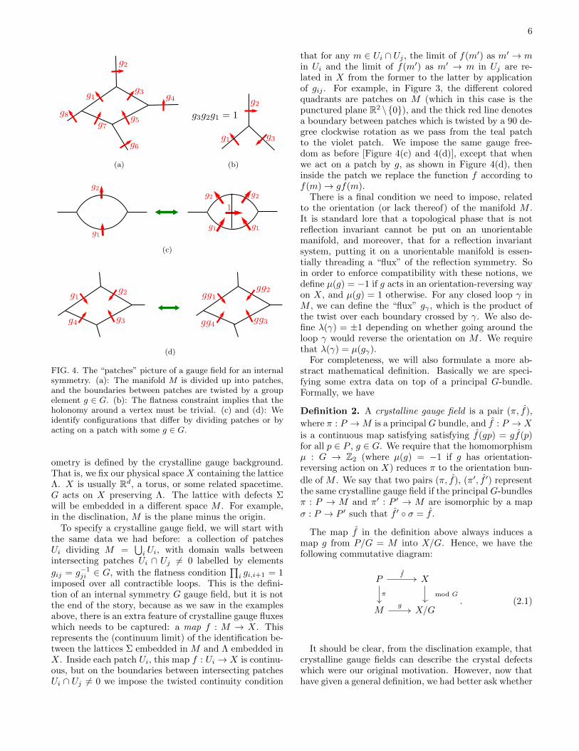
To further motivate the definition, let us recall the def-inition of a gauge field for an internal (discrete) sym-metry. Gauge fields for discrete symmetries are some-what more esoteric than gauge fields for continuousgroups (like the familiar electromagnetic vector potentialAµ). One way to think about them is that they encode“twisted boundary conditions”. For example, threadinga non-trivial gauge flux for an Ising symmetry through asystem living on a circle means that we make a cut andidentify spin-up on one side of the cut with spin-down onthe other side of the cut (“anti-periodic boundary condi-tions”). In general, to specify a gauge field on a manifoldM we can build M up out of “patches”. The boundariesbetween patches (“domain walls”) are “twisted” by anelement g ∈ G of the symmetry group (“transition func-tions”), which tells us how to identify the patches. Adiscrete gauge field must be “flat”, which is to say therecan be no non-trivial holonomy around a vertex whereseveral patches intersect, as shown in Figure 4. This is tosay there is no G-flux through the vertices (or along suchline-like junctions in a 3d picture). There is some inher-ent gauge freedom: firstly, we can merge or split patches,provided that the boundaries thus created or destroyedare twisted by the trivial element 1 ∈ G; secondly, wecan apply an element gp ∈ G of the symmetry group toa given patch p, which has the effect of multiplying the

FIG. 3. A 90 degree disclination maps discontinuously to thesquare lattice, as indicated with the colored quadrants. Thered line is the branch cut across which the image rotates by90 degrees. Because the discontinuity is by a rotation in G,this map descends to a continuous map from the disclinationto the quotient of the square lattice by G.

twist carried by the boundaries of this patch by gp. Thisgauge freedom relates two different representations of thesame gauge field. More abstractly (but equivalently), wecan define a gauge field as a principal G-bundle over M[66].

As an example, we can consider a g-flux at the ori-gin of the plane. This g-flux is defined as a G gaugefield on the plane minus the origin. It may be definedusing a single (simply-connected) patch which meets it-self along a domain wall extending from the origin toinfinity. This domain wall is labeled with the transitionfunction g, indicating that a point charge taking along apath encircling the origin will return to its original po-sition with any internal degrees of freedom transformedby the symmetry g. The similarity between the internalsymmetry flux and the crystal defect is striking. It leadsus to identify the role of the branch cut in the latter withthe domain wall of the former.

With this identification in hand, we are ready to stateour definition of crystalline gauge field, by directly gen-eralizing the patches picture of internal symmetry gaugefields. An important novelty will be that the lattice ge-

6

(a) (b)

(c)

(d)

FIG. 4. The “patches” picture of a gauge field for an internalsymmetry. (a): The manifold M is divided up into patches,and the boundaries between patches are twisted by a groupelement g ∈ G. (b): The flatness constraint implies that theholonomy around a vertex must be trivial. (c) and (d): Weidentify configurations that differ by dividing patches or byacting on a patch with some g ∈ G.

ometry is defined by the crystalline gauge background.That is, we fix our physical space X containing the latticeΛ. X is usually Rd, a torus, or some related spacetime.G acts on X preserving Λ. The lattice with defects Σwill be embedded in a different space M . For example,in the disclination, M is the plane minus the origin.

To specify a crystalline gauge field, we will start withthe same data we had before: a collection of patchesUi dividing M =

⋃i Ui, with domain walls between

intersecting patches Ui ∩ Uj 6= 0 labelled by elements

gij = g−1ji ∈ G, with the flatness condition

∏i gi,i+1 = 1

imposed over all contractible loops. This is the defini-tion of an internal symmetry G gauge field, but it is notthe end of the story, because as we saw in the examplesabove, there is an extra feature of crystalline gauge fluxeswhich needs to be captured: a map f : M → X. Thisrepresents the (continuum limit) of the identification be-tween the lattices Σ embedded in M and Λ embedded inX. Inside each patch Ui, this map f : Ui → X is continu-ous, but on the boundaries between intersecting patchesUi ∩ Uj 6= 0 we impose the twisted continuity condition

that for any m ∈ Ui ∩ Uj , the limit of f(m′) as m′ → min Ui and the limit of f(m′) as m′ → m in Uj are re-lated in X from the former to the latter by applicationof gij . For example, in Figure 3, the different coloredquadrants are patches on M (which in this case is thepunctured plane R2 \0), and the thick red line denotesa boundary between patches which is twisted by a 90 de-gree clockwise rotation as we pass from the teal patchto the violet patch. We impose the same gauge free-dom as before [Figure 4(c) and 4(d)], except that whenwe act on a patch by g, as shown in Figure 4(d), theninside the patch we replace the function f according tof(m)→ gf(m).

There is a final condition we need to impose, relatedto the orientation (or lack thereof) of the manifold M .It is standard lore that a topological phase that is notreflection invariant cannot be put on an unorientablemanifold, and moreover, that for a reflection invariantsystem, putting it on a unorientable manifold is essen-tially threading a “flux” of the reflection symmetry. Soin order to enforce compatibility with these notions, wedefine µ(g) = −1 if g acts in an orientation-reversing wayon X, and µ(g) = 1 otherwise. For any closed loop γ inM , we can define the “flux” gγ , which is the product ofthe twist over each boundary crossed by γ. We also de-fine λ(γ) = ±1 depending on whether going around theloop γ would reverse the orientation on M . We requirethat λ(γ) = µ(gγ).

For completeness, we will also formulate a more ab-stract mathematical definition. Basically we are speci-fying some extra data on top of a principal G-bundle.Formally, we have

Definition 2. A crystalline gauge field is a pair (π, f),

where π : P →M is a principal G bundle, and f : P → X

is a continuous map satisfying satisfying f(gp) = gf(p)for all p ∈ P , g ∈ G. We require that the homomorphismµ : G → Z2 (where µ(g) = −1 if g has orientation-reversing action on X) reduces π to the orientation bun-

dle of M . We say that two pairs (π, f), (π′, f ′) representthe same crystalline gauge field if the principal G-bundlesπ : P → M and π′ : P ′ → M are isomorphic by a map

σ : P → P ′ such that f ′ σ = f .

The map f in the definition above always induces amap g from P/G = M into X/G. Hence, we have thefollowing commutative diagram:

P X

M X/G

f

π mod G

g . (2.1)

It should be clear, from the disclination example, thatcrystalline gauge fields can describe the crystal defectswhich were our original motivation. However, now thathave given a general definition, we had better ask whether

7

all crystalline gauge fields admit such a physical inter-pretation. In particular, there ought to be a well-definedsense of what it means to couple to a general crystallinegauge field.

For internal symmetries it is familiar how to coupleto a gauge field, at least when that gauge field lives onM = X. Given a gauge field A for a (discrete) inter-nal symmetry G, described using patches and transitionfunctions, and given a Hamiltonian H that commuteswith the symmetry, we can define a Hamiltonian H[A]that describes the system coupled to the gauge field. Todo this, we assume that H can be written as a sum oflocal terms. Then, H[A] contains a local term for eachlocal term in H. The terms in H which act only within apatch carry over to H[A] without change, while for termsin H which act in multiple patches, we must first performa gauge transformation so that the term acts in a singlepatch, add it to the Hamiltonian, and then reverse thatgauge transformation. See, for example [7].

Now suppose that we want to do the same thing forcrystalline gauge fields. For crystal defects (for example,the disclination in Figure 3) it should be clear how todo this; locally, the defect lattice looks the same as theoriginal lattice, so we just pull local terms in X backinto M . On the other hand, this construction doesn’tnecessarily work for a general crystalline gauge field. Wehave to impose a condition which we call rigidity.

Definition 3. A crystalline gauge field (expressed interms of patches, twisted boundary conditions, and amap f : M → X) is rigid if near any point m ∈ M thatmaps into a lattice point in X under f , there exists a lo-cal neighborhood U containing m such that, after makinga gauge transformation such that U is contained in a sin-gle patch, f is injective (one-to-one) when restricted toU ; and, moreover, the image of U under f contains alllattice points that are coupled to f(m) by a term in theHamiltonian.3

This somewhat technical definition is best understoodby considering examples of crystalline gauge fields whichare not rigid. An extreme example is the case wheref : M → X is the constant function: there is somex∗ ∈ X such that f(m) = x∗ for all m ∈ M . In otherwords, every point in M gets identified with a single pointin X. If the Hamiltonian in X has terms coupling x∗ withsome other nearby point, then there is no way to definecorresponding terms acting in M , since the nearby pointdoes not correspond to any point in M . More generally,rigidity fails when there are points at which f is not lo-cally invertible; if f is a smooth map between manifolds,this is equivalent to saying that there are points at whichits Jacobian vanishes.

3 For certain applications, this last condition may be relaxed neara boundary of M . Terms in the Hamiltonian which fall of theedge may need to be discarded or modified in some arbitrarymanner.

For a rigid crystalline gauge field, on the other hand,there is always a well-defined procedure to couple it to theHamiltonian. The idea is that rigidity guarantees thatthe local neighborhood is always sufficiently well-behavedthat it makes sense to pull terms in the Hamiltonian fromX back into M . This is illustrated in Appendix C

Finally, let us remark on a interesting property of thethe definition of crystalline gauge field: in the case thatthe whole symmetry group acts internally (that is, theaction of G on X is trivial), we might have expected thedefinition to reduce to the usual notion of a gauge field foran internal symmetry. However, this is evidently not thecase, because there is still the map f : M → X (which inthis case must be globally continuous). We believe that,in fact, this may be a more complete formulation of agauge field for an internal symmetry.

B. Crystalline topological liquids

From the discussion in the preceding discussion, itmight seem that we should only consider rigid crystallinegauge fields. Now, however, we want to argue that thisis too restrictive. One indeed should require a crys-talline gauge field A to be rigid if one wants to go froma Hamiltonian H to a Hamiltonian H[A] coupled to A.But such a microscopic lattice Hamiltonian is a prop-erty of the system in the ultra-violet (UV). On the otherhand, when classifying topological phases, what we actu-ally care about is the low-energy limit. The central con-jecture of this work is that it is well-defined to discuss thelow-energy topological response to any crystalline gaugefield (not just a rigid one).

One reason for this is that a spatially-dependent TQFTthat is invariant under a spatial symmetry can be ex-pressed as a single TQFT coupled to a background fieldwhich is precisely our crystalline gauge background of Def2 (with no rigidiy constraints)! This should be comparedwith the result for internal G symmetry which says thata G action on a (single) TQFT is equivalent to a TQFTwith an ordinary background G gauge field. In otherwords, topological field theories can be gauged and theresulting topological gauge theory retains all the informa-tion of the original theory and its symmetry action[67]4.We discuss this further in section V.

Such considerations provide the mathematical basis forour conjecture about the gauge response. Nevertheless,since these arguments are very abstract and potentiallyunappealing to readers not familiar with TQFTs, wewill also give a more concrete prescription for couplingsmooth states (recall that we introduced this concept inSection I) to a general crystalline gauge field. For sim-plicity, we will only consider the case where there are

4 In the mathematics literature, this is often stated “equivarianti-zation is an equivalence”.

8

no orientation-reversing symmetries, although we expectthat this restriction can be lifted.

The idea is that there is a simple set of data whichone can use to specify a smooth state. Firstly, in theneighborhood of every point in space, we need to spec-ify the orientation of the fine lattice; this can be spec-ified through a framing of the manifold M (i.e. a con-tinuous choice of basis for the tangent space at everypoint). Moreover, in the neighborhood of every point inspace, the state looks like it respects the (orientation-preserving) spatial symmetries of the fine lattice (glob-ally, of course, this is not the case). Hence, there is amap ψ : M → Ω, where Ω is the space of all groundstates invariant under the spatial symmetries of the finelattice. (For our arguments, it won’t be important tocharacterize Ω precisely). For a smooth state, we requirethis map to be continuous.

As a warm-up, we will first show how to define couplingto a gauge field for an internal discrete unitary symmetryG in terms of smooth states. Let Ω be a space of groundstates, with G acting on Ω as a tensor product over everysite, with the action at a given site described by the rep-resentation u(g). Let ψ ∈ Ω be a G-invariant state. Now,given a framed manifold M and a G gauge field A (i.e.collection of patches on M with G-twisted boundary con-dition; alternatively, a principal G-bundle over M), wewill show how to define a smooth state ψ[A] : M → Ω.For each g we define a continuous path u(g; t), t ∈ [0, 1]such that u(g; 0) = I and u(g; 1) = u(g). Given thatψ is G-invariant, acting with [u(g; t)]⊗N on ψ defines aloop ψg(t) ∈ Ω, such that ψg(0) = ψg(1) = ψ. Then,inside each patch we just set ψ[A](m) = ψ. But we deco-rate patch boundaries twisted by a group element g ∈ Gby the corresponding loop. That is, we require that, asm crosses such a boundary, ψ[A](m) goes through theloop described by ψg(m; t). One might wonder whetherthis procedure is well-defined at the intersections betweenpatch boundaries. For example, an obstruction would oc-cur if the composition of the paths ψg1 , ψg2 and ψ(g1g2)−1

defines a non-contractible loop, i.e. a non-trivial elementin the fundamental group π1(Ω). In Appendix D, weshow that such obstructions can never arise, providedthat we sufficiently enlarge the on-site Hilbert space di-mension. We also give a more rigorous formulation interms of the classifying space BG.

Now we return to the case of a crystalline gauge field,but by way of simplification we first consider the casewhere there is no symmetry. Then a crystalline gaugefield A on a manifold M is simply a continuous mapf : M → X. In general, there is no way to define theHamiltonian H[A]. But for a smooth state ψ : X →Ω there is a well-defined way to define a correspondingsmooth state ψ[A] : M → Ω which describes ψ coupledto A. Indeed, we just define ψ[A](m) = ψ(f(m)). (Tocompletely specify the state, we also have to choose aframing on M). This should be compared with Kitaev’s“weak symmetry breaking” paradigm[68], where our Ωplays the role of Kitaev’s Y .

Finally, we can combine the ideas from the previoustwo paragraphs to give a prescription for coupling asmooth state to a crystalline gauge field for a symmetryG acting on X, living on a manifold M . The crystallinegauge field is specified (according to the discussion in Sec-tion II A) by a collection of patches on M with twistedboundaries, and a function f : M → X respecting thetwisted boundary conditions. We assume the symmetryaction takes the form U(g) = S(g)[u(g)]⊗N , where S(g)is a unitary operator that simply permutes lattice sitesaround according to the spatial action, and [u(g)]⊗N is anon-site action. Then we define a path u(g; t) for t ∈ [0, 1]such that u(g, 0) = I, u(g, 1) = u(g). By acting with[u(g; t)]⊗N we obtain a path ψg(x; t) in M . It’s not aloop this time, though; instead G-invariance of ψ impliesthat ψg(x; 0) = ψ(x), ψg(x; 1) = ψ(gx). Now we can de-fine the coupled state ψ[A] as follows. Inside each patch,we have ψ[A](m) = ψ(f(m)). Then, for patches con-nected by boundaries twisted by g ∈ G, we connect upthe ψ[A] in the respective patches by means of the pathsψg(x; t). The previously noted endpoints of these pathsare consistent with the fact that f(m) jumps to gf(m)as one crosses the boundary. Again, we defer the proofthat this procedure is well-defined at the intersection ofboundaries to Appendix D.

At this point, the careful reader might raise an objec-tion. In our statement of the conjecture about couplingto a crystalline gauge field, we did not require the man-ifold M to be framed, only orientable (the orientabilitycondition comes from our stipulation that there are noorientation-reversing symmetries, and from the compati-bility condition between the orientation bundle of M andthe crystalline gauge field discussed in Section II A andagain in Section V). But so far, our smooth state argu-ments only showed how to couple to crystalline gaugefields on framed manifolds. There are two questions thatstill need to be addressed:

• Question 1. Does the topological response dependon the choice of framing?

• Question 2. Can the topological response be de-fined on oriented manifolds that do not admit aframing?

These questions need to be addressed in any formula-tion of continuum limit. For bosonic systems we expectthat the continuum limit, if it exists, can be defined onany oriented manifold and doesn’t depend on any extrastructure. For fermionic systems it also can depend ona spin or spinc structure. There are of course systemswhich, while gapped, still exhibit some metric or fram-ing dependence in the IR, eg. Witten’s famous framinganomaly of Chern-Simons theory [69]. We will later ap-proach these questions in the TQFT framework of sectionV. For now let us think about these questions from theperspective of smooth states.

For Question 1, we observe that that changing theframing corresponds to changing the fine lattice, and

9

generally speaking, most topological phases have a “liq-uidity” property that ensures that the ground states ondifferent lattices can be related by local unitaries. Sincethe states live on different lattices, this requires bring-ing in and/or removing additional ancilla spins that arenot entangled with anything else, as is standard protocolwhen defining local equivalence of quantum states. Sucha liquidity property will be necessary for the crystallinetopological liquid condition to be satisfied. There aresome notable exceptions, such as fracton phases [61], ofwhich a simple example is a stack of toric codes. We donot expect such fracton phases to be crystalline topolog-ical liquids.

As for Question 2, we believe that the answer is prob-ably yes. To illustrate the issues at play, consider the 2-sphere. This is an orientable 2-manifold which does notadmit a framing. As a consequence, there is no way toput a regular square lattice on a 2-sphere; there must beat least a singular face which is not a square or a singularvertex which is not 4-valent. So one cannot strictly de-fine a smooth state. But we expect that there are ways to“patch up” such singular points so that they don’t affectthe long-range topological response. For example, thetoric code is usually defined on a square lattice, whichcannot be placed onto the sphere, but it is easy to puta toric-code-like state on the sphere by allowing a fewnon-square faces.f

We emphasize that coupling to non-rigid crystallinegauge fields is what allows us to establish the crystallineequivalence principle. For example, for internal symme-tries one could consider braiding symmetry fluxes aroundeach other. Does this make sense in the case of, for ex-ample, disclination defects? If the disclinations were in-terpreted strictly as lattice defects this would not be pos-sible, since there is no continuous deformation of a latticecontaining two disclinations such that the two disclina-tions move around each other with the lattice returningto its original configuration. But if we interpret discli-nation defects as special cases of (generally non-rigid)crystalline gauge fields, then this braiding process is al-lowed. The physical interpretation is that in the course ofthe braiding process, additional sites get coupled to, andsuperfluous sites decoupled from, the system by meansof local unitaries (as discussed above in the context ofthe framing dependence). That is, the lattice geometrychanges along the path.

In conclusion, this discussion motivates our terminol-ogy of “crystalline topological liquid”: although such sys-tems are “crystalline” in the sense that they have spa-tial symmetries, they are also “topological liquids” inthe sense that the lattice is not fixed but can be trans-formed into other geometries by means of local unitaries(with ancillas). This is also consistent with our picturefrom Section I that the topological response of crystallinetopological liquids “forgets” about the lattice.

C. The Crystalline Equivalence Principle

Most of the time, we will be interested in topologicalcrystalline phases in Euclidean space X = Rd. Moreover,the topological response should only depend on the de-formation class of the crystalline gauge field. It turns outthat for X = Rd there is a very simple characterizationof the collapsible homotopy classes of crystalline gaugefields:

Theorem 1. If X is contractible (e.g. X = Rd), thenthe deformation classes of crystalline gauge fields are inone-to-one correspondence with internal gauge fields.

That is, in the “patches” formulation of crystallinegauge fields, the deformation classes remember only thetwisted boundary conditions and not the function f :M → X. This theorem is a corollary of the more generalclassification theorem for crystalline gauge fields. SeeThm 6. However, here we remark on an elementary wayto see one part of Thm 1: namely, that homotopy classescan only depend on the twisted boundary conditions.(For the moment we will not attempt to prove the otherpart, namely that any configuration of twisted bound-ary conditions has at least one function f respecting it).Although the proposition holds more generally, for sim-plicity we consider the case where X = Rd and where theG action on X is affine linear:

gx = Agx+ bg, (2.2)

where Ag is a (d × d) matrix and bg is a length d vec-tor. We then observe that given a patch configurationon M with twisted boundary conditions, and two mapsf0 : M → X and f1 : M → X respecting the sametwisted boundary conditions, then there is a continuousinterpolation

fs = (1− s)f0 + sf1, (2.3)

which respects the same twisted boundary conditions allthe way along the path.

Thm 1 allows us to deduce the most important resultof this paper. Thm 1 shows that deformation classes ofcrystalline gauge fields are in one-to-one correspondencewith principle G-bundles. On the other hand, deforma-tion classes of gauge fields for an internal symmetry alsocorrespond to principal G-bundles. Topological phasesare distinguished by their response to background gaugefields. Therefore we conclude the

Crystalline Equivalence Principle: The clas-sification of crystalline topological liquids on a con-tractible space with spatial symmetry group G is thesame as the classification of topological phases withinternal symmetry G.

To be precise, the orientation-reversing symmetries onthe spatial side are identified with the anti-unitary sym-metries on the internal side. Further, in fermionic sys-tems, reflections with R2 = 1 correspond to time reversal

10

with T 2 = (−1)F and vice versa. (These statements arenot clear from the above treatment since we haven’t dis-cussed gauging anti-unitary symmetries. However, theyfollow from the general TQFT picture, as discussed inV A).

D. Beyond Euclidean space

Before we delve into the details of how to classify crys-talline topological liquids by their topological responseto gauge fields, we recall that the above considerationsrefer to topological phases that exist in Euclidean spaceRd. In principle one can consider the more exotic prob-lem of classifying topological phases on non-contractiblespaces; for example, the d-sphere, the d-torus, or a Eu-clidean space with holes5. The practical relevance of thisproblem may be a bit obscure, but from a theoreticalpoint of view we find it more enlightening to formulatethe problem we are interested in – Euclidean space – asa special case of the more general problem. It also il-lustrates an important conceptual point, because, as weshall see, the Crystalline Equivalence Principle does nothold on non-contractible spaces (see, for example, Sec-tion VI). Thus, the Crystalline Equivalence Principle isnot something that a priori had to be true. Rather, it isa consequence of the fact that systems of physical interestlive in Euclidean space.

On contractible spaces, we had the classification The-orem 1 for crystalline gauge fields. This classificationtheorem is a special case of the more general result (seeAppendix E and Theorem 6) that deformation classes ofcrystalline gauge fields M → X are classified by homo-topy classes of maps from M into the “homotopy quo-tient” X//G, pronounced “X mod mod G”. For X con-tractible, X//G is homotopic to the “classifying space”BG, so we recover Theorem 1 if we invoke the well-knownfact that principal G-bundles over M are classified by ho-motopy classes of maps M → BG.

III. EXACTLY SOLVABLE MODELS

It is of course important to show that we can explicitlyconstruct Hamiltonians realizing topological crystallinephases classified in this work. We do this using a “boot-strap” construction. This is really a meta-construction,in the sense that it is a prescription for going from aconstruction for an SPT or SET phase with internalsymmetry to a construction for a topological crystallinephase. A similar idea was used by one of us to construct

5 We emphasize that, in the absence of translation symmetry, itdoes not make sense to relate a topological phase defined on onecompact space to one defined on another space with differenttopology. That is, the classification can depend on the back-ground space.

phases of matter protected by time-translation symmetryin Ref. 63.

For simplicity we consider the case where the entiresymmetry group G acts spatially, i.e. the internal sub-group is trivial. We will also consider the case where Gdoes not contain any orientation-reversing transforma-tions, and we work in Euclidean space, X = Rd. First ofall, let ϕ be a surjective homomorphism from the sym-metry group G to a finite group Gf . We use one of manyapproaches to construct a topological liquid with an in-ternal symmetry Gf . In most of these approaches, thereis no obstacle to construct the Hamiltonian to also havea spatial symmetry G, which commutes with Gf so that

the full symmetry group is G = G × Gf (for example,in the case of bosonic SPTs, this can be shown explicitlyusing the construction of Ref. [17], as detailed in Ap-pendix F). We then can imagine deforming Hamiltonian

to break the full symmetry group G down to the diagonalsubgroup

G′ = (g, ϕ(g)) ∈ G ∼= G. (3.1)

We expect that this model will be in the topological crys-talline phase that corresponds to the internal symmetry-protected phase we started with via the crystalline equiv-alence principle. Indeed, we can do this construction ona lattice with lattice spacing much less than the unit cellsize (thus giving a smooth state), and verify that, for the

original model (without the G-breaking perturbation),following the prescription given in Section II A to coupleto a crystalline gauge field for the diagonal subgroup G′

gives the same result as coupling to an internal gaugefield for the internal subgroup G. (A similar argumentcan be given in the spatially-dependent TQFT picture ofSection V).

Let us briefly sketch how to extend the above con-struction to symmetry groups G containing orientation-reversing transformations. A general topological phaseis not reflection-invariant, so the above argument needsto be modified. We expect that a topological liquidcan always be made invariant under a spatial symme-try G if we make the orientation-reversing elements ofG act anti-unitarily ; we can call this suggestively the“CPT princple”6 We prove this explicitly for bosonicSPT phases in Appendix F. We then proceed as be-fore, starting from a (G × Gf )-symmetric topologicalphase, where the internal symmetry ϕ(g) ∈ Gf actsanti-unitarily if g was orientation-reversing. Then even-tually the symmetry gets broken down to the diagonalsubgroup G′, which contains spatial symmetries, possi-bly orientation-reversing, but all acting unitarily (since

6 This is related to, but not a consequence of, the CPT theorem,because here we are talking about lattice models, not relativisticquantum field theories. The CPT principle doesn’t claim thatevery lattice model is CPT invariant, which would be demon-strably false; rather, it posits that in any topological phase thereis at least one CPT-invariant point.

11

the orientation-reversing elements of G, which we havetaken to act anti-unitarily, get paired with anti-unitaryelements of Gf ). We expect that this gives the topologi-cal crystalline phase corresponding to the original inter-nal symmetry-protected phase via the crystalline equiva-lence principle, but explicitly determining the topologicalresponse would involve explaining what it means to gaugean anti-unitary symmetry, which we will not attempt todo (but see Ref. 70.)

IV. TOPOLOGICAL RESPONSE ANDCLASSIFICATION

In this section, we will discuss how our understand-ing of what it means to gauge a spatial symmetry al-lows us to classify topological phases by their topolog-ical responses. Basically, any approach to understand-ing topological phases with internal symmetries whichrelies on gauging the symmetry, can be applied equallywell to space-group symmetries by coupling to crystallinegauge fields. Moreover, in Euclidean space, Theorem 6should imply that we obtain the same classification as forinternal symmetries, in accordance with the CrystallineEquivalence Principle. In non-contractible spaces we mayobtain a different classification.

There are two main approaches to thinking about topo-logical response. The first is a bottom-up approach whereone starts with a Hamiltonian in a lattice model and oneattempts to work out all the topological excitations. Forexample in 2+1D, one has anyons and symmetry fluxesand one can ask about how they interact. This is tabu-lated mathematically in a G-crossed braided fusion cate-gory [7, 71] and one can try to work out a classification ofthese objects or at least find some interesting examplesand then look for lattice realizations.

The second approach is a top-down one where one firstassumes the existence of a low energy and large systemsize (”IR”) limit of the gapped system. This is a topolog-ical quantum field theory (TQFT) of some sort and onecan just try to guess what it is from the microscopic sym-metries, entanglement structure (short-range vs. long-range), and so on. One can make a bold statement thatall possible IR limits are of a certain type of TQFT andthen try to classify all of those. Despite its obvious lackof rigor, this approach has proven successful.

One reason for this is that it is often possible tobridge the two perspectives. For example, a G-SPTcan be understood in terms of an effective action ω ∈HD+1(BG,Z)[17, 57] leading ultimately to a TQFT. Butconsidering the fusion of symmetry fluxes also leads to anelement of HD(G,U(1)) through a higher associator ofsymmetry fluxes (in 2 + 1-D, it is the F symbol). Theseare equivalent under the isomorphism HD+1(BG,Z) =HD(G,U(1)) (see Appendix A for more explanation ofthis isomorphism). In general, defects such as anyons andsymmetry fluxes can be described in the TQFT frame-work through the language of “extended TQFT”.

Let us now discuss how these methods can be extendedto the case of spatial symmetries.

A. Flux fusion and braiding for SET phases in(2+1)-D with spatial symmetry

If we want to classify symmetry-enriched phases in(2+1)-D phases we can consider the “bottom-up” ap-proach of Ref. 7. There, one has a topological phasewith an internal symmetry G, and one envisages cou-pling to a classical background gauge field. In particu-lar, one can consider gauge-field configurations in whichthe gauge fluxes are localized to a discrete set of points.One can then consider the algebraic structure of braid-ing and fusion of such gauge fluxes, which is an exten-sion of the braiding and fusion of the intrinsic excitations(anyons) that exist without symmetry. This structure isargued to be described by a mathematical object calleda “G-crossed braided tensor category”. For a crystallinetopological liquid on Euclidean space, we expect thatthe equivalence between crystalline gauge fields and G-connections allows the arguments to carry over withoutsignificant change. (We will leave a detailed derivationfor future work.) On non-contractible spaces, presum-ably a generalization of the arguments of Ref. 7 shouldbe possible, but we will not explore this.

B. Topological Response as Effective Action

Another way to compute topological response, whichdoes not involve braiding or fusing fluxes is by computingtwisted partition functions. That is, given a backgroundgauge field (ordinary or crystalline) A on a spacetime M ,we can compute the partition function of Z(M,A) andcompare it to the untwisted partition function Z(M).The assumption is that

Z(M,A)/Z(M)

tends to a complex number of modulus 1 in the limitthat M becomes very large compared to the correlationlength. In favorable situations, such as a crystalline topo-logical liquid, the limiting phase is a topological invari-ant of M and its gauge background A. We call this thetopological response of our system to A and its log theeffective action for the gauge background A. In somecases, like M = Y × S1, Z(M,A) can be interpreted assome kind of “twisted trace” of symmetry operators, aswe soon discuss. In general there is such an interpre-tation but it involves topology-changing operators [72].7. What is most important for classification of phasesis that it is a number that captures some (or all) of the

7 Indeed, on a general spacetime, a generic choice of time directiondefines a Morse function and a foliation of spacetime by spatial

12

data in a “spatially-dependent TQFT”, which we intro-duce in Section V as the mathematical way to describe a“crystalline topological liquid” phase of matter.

For internal symmetries of bosonic systems, we knowthat in this case, the limiting ratio can be written

Z(M,A)/Z(M)→ exp

(2πi

∫M

ω(A)

), (4.1)

where ω(A) is a gauge-invariant top form made out ofthe gauge field. In the case of a crystalline gauge field

A = (P,M, π, f), we will also assume that the topologicalresponse is an exponentiated integral:

Z(X,A)/Z(X)→ exp

(2πi

∫M

ω(α, f)

), (4.2)

where ω(α, f) is a top form on M made of the twistingfield α ∈ H1(M,G) which classifies the cover P and the

map f , used to pull back densities from X. In the casethat G is purely internal, α plays the role of A in (4.1).

As discussed in Ref 57, responses of the form (4.1) arethe same thing as cocycles in group cohomology, definedas cohomology of the classifying space HD(BG,U(1))8,where D is the dimension of spacetime X. This re-produces the classification of internal symmetry bosonicSPTs in Ref 17. To construct the effective action of A,we use the fact that the gauge field A itself is the sameas a map A : X → BG, and given a D-cocycle on BG,we can pull it back along this map to get ω(A) over X.

Analogously, we can think of our crystalline gauge fieldas a map A : M → X//G (see Appendix E) and take anyform in HD(X//G,U(1)), pull it back along this map

to M to get a ω(α, f) and integrate it (see AppendixG). We just need to be a little careful with coefficients.We intend to integrate ω(α) over M , but if G containsorientation-reversing elements like mirror and glide re-flections (or time reversal), then M may likely be un-orientable. Integration on an unorientable M is doneby choosing a local orientation: orienting M away fromsome hypersurface N and performing the integration onM −N with its orientation. To ensure the integral doesnot depend on this local orientation, we need our topform ω(α) to switch sign with the local orientation isreversed. Mathwise, this means that ω(α) should livein cohomology HD(M,U(1)or) with twisted coefficientsU(1)or. Luckily, if X is orientable, then the unorientabil-ity of M is entirely due to orientation-reversing elementsof G, so if we use twisted cohomology HD(X//G,U(1)or)

slices. At critical points of this Morse function, the spatial sliceis singular and we have a topology changing operator that getsus from the Hilbert space just before the critical point to theHilbert space just after. These are all handle attachments andcan be thought of as generalized flux fusion processes.

8 Actually we should use only measurable cohomology or use differ-ent coefficients in a different degree: HD+1(BG,Z). We discussthis subtlety in Appendix A.

where orientation-reversing elements of G act on U(1)by θ 7→ −θ, then the coefficients will pull back properly.This cohomology group is well known in algebraic topol-ogy as the equivariant cohomology of X, and is written

HDG (X,U(1)or) := HD(X//G,U(1)or).

Another subtlety comes from considering the identitymap M = X → X as a crystalline gauge field. Anynon-trivial topological response to the identity cover isequivalent to a shift of all the partition functions by aphase. We may as well consider only the subgroup of allequivariant cohomology classes which pulled back alongthe identity map are trivial. This is called reduced coho-mology and is denoted with a tilde H.

Summarizing (and recalling the subtlety about replac-ing U(1)→ Z increasing the degree by 1, as discussed inAppendix A ), we find:

Theorem 2. Homotopy-invariant effective actions inD = d + 1 spacetime dimensions for crystalline gaugefields A : M → X//G which may be written as inte-grals over M are in correspondence with “twisted reducedequivariant cohomology”:

HD+1G (X,Zor).

In the following section, we will give examples of crys-talline SPT states and how to compute the topologicalresponse as a class in equivariant cohomology.

Finally, even though these are all the effective actions,from what we’ve learned in the case with time rever-sal symmetry[21] and consideration of thermal Hall re-sponse, we know these are very unlikely to be all thephases. There are some criteria, like homotopy invari-ance, that pick out these phases based on their effectiveaction, but we don’t know a microscopic characterizationof which phases come from group cohomology and whichphases are from the beyond. We say “bosonic” becausewe have learned the importance of including spin struc-ture in a careful way [27]. We discuss the relationshipbetween topological actions and phases in Appendix A.

C. Examples of Topological Response

Let us explain in some examples how the topologicalresponse (4.2) manifests itself physically and how it canbe computed starting from an SPT state. These exam-ples were constructed using the techniques in AppendixF.

1. Reflection SPT in 1+1D

We consider a system of spin-1/2’s lying along the x-axis at integer coordinates x = j. We will use the Xbasis for these spins and consider the state

· · · | ←〉 ⊗ | ←〉 ⊗ (| →〉 − | ←〉)⊗ | →〉 ⊗ | →〉 · · · .

13

There is no reflection-symmetric perturbation (keepingthe gap) which can take that central minus sign to a plus.This is because it can be understood as an odd chargefor an internal Z2 symmetry induced by reflection at thereflection center. This odd charge is the signature of thisSPT phase. Let us see how to compute it as a topologicalresponse.

Observe that this odd charge can be detected using atrace

charge at reflection center = limβ→∞

Tr R e−βH′

= −1,

(4.3)where H is a gapped Hamiltonian with ground state asabove and R is the reflection operator. Traces are com-puted by path integrals with a periodic time coordinate.The insertion of R means that as we traverse this peri-odic time, we come home reflected. This means that thegeometry of the spacetime whose path integral computesthis trace is a Mobius strip.

We can represent this geometry as a crystalline gaugefield over

X = Rx × S1t = (x, t)|x ∈ R, t ∈ [0, 1], (x, 0) = (x, 1),

the usual domain for background gauge fields used tocompute twisted traces. We write the Mobius strip

M = (m, s)|m ∈ R, s ∈ [0, 1], (m, 0) = (−m, 1).

We get a continuous map

f(m, s) = (|m|, s) : M → X/R,

where

X/R = (x, t)|x ∈ R, t ∈ [0, 1], (x, 0)

= (x, 1), (x, t) = (−x, t).

There is no continuous lift of this map to X, so we inserta branch cut along s = 0 in M . This defines a coveringspace

P = (m, s′)|m ∈ R, s′ ∈ [0, 2], (m, 0) = (m, 2)

with covering map π : P →M defined by

π(m, s′) =

(m, s′) 0 ≤ s′ ≤ 1

(−m, s′ − 1) 1 ≤ s′ ≤ 2

This has a map f : P → X defined by

f(m, s′) =

(m, s′) 0 ≤ s′ ≤ 1

(m, s′ − 1) 1 ≤ s′ ≤ 2

We summarize with a diagram (cf. Defn (2.1))

P X

M X/R

f

π (|x|,t)

f . (4.4)

The trace (4.3) is therefore interpreted as a topologicalresponse −1 to this crystalline gauge field is −1 a la (4.2)and we would like to write it in the form

∫ω(α) for some

ω ∈ H2(BZ2, U(1)or), where α is our double cover π :P → M interpreted as a Z2 gauge field which tells uswhere the branch cuts are. It turns out there is a uniquenon-trivial class ω(α) = 1

2α2 and indeed if we compute

(with particular boundary conditions)

exp

(2πi

1

2

∫M

α2

)= −1

we reproduce the trace (4.3).Before we move on to richer examples, let us make

some comments for the mathematically inclined on theevaluation of this integral. To get the claimed answer,we used the one-point-compactification of M , where weadd a single point at infinity, collapsing the boundaryto a point. The one-point-compactification of M is theprojective plane RP2 and the usual integral

∫RP2 α2 = 1.

There is, however, no rigid crystalline gauge field overX with M = RP2 since X is noncompact. However,if we impose R-symmetric, time independent boundaryconditions on our crystal, then our cylindrical spacetimeRx × S1

t gets each end collapsed to a point and becomesa sphere. The reflection group continues to act on thissphere and there is a rigid crystalline gauge field withM = RP2 over S2.

In computing more complicated examples of this sameSPT phase (examples which are not already disentan-gled), indeed one finds it necessary to choose someboundary conditions in (4.3) to get a nonzero trace.What if we use periodic boundary conditions? In thatcase, there is always a reflection center at ∞, and peri-odicity implies that the reflection center will also carry anodd charge. Therefore, the trace with periodic boundaryconditions will receive a contribution from both reflec-tion centers and be (−1)2 = 1. We can see this with ourcrystalline gauge fields. Indeed, with periodic boundaryconditions spacetime becomes a torus S1

x × S1t and if we

insert a reflection twist in the time direction we obtainM as a Klein bottle. We identify α with the orientationclass in H1(M,Z2) = Z2⊕Z2 and for this class α2 = 0, asexpected! On the other hand, one can use Mobius bandscentered at either reflection center to see the odd chargeat each one. Gluing them along their overlap gives us theKlein bottle again and the partition functions multiply9.We will see this in more detail in the following example.

2. Reflection and Translation in 1+1D

Next we consider a one-dimensional system with atranslation and a reflection symmetry. In particular, the

9 This is a form of cobordism invariance.

14

state ⊗j∈Z

(| ←〉+ (−1)j | →〉).

This state is symmetric under reflection around 0:R0(x) = −x, and also under reflection around 1:R1(x) = 2− x. The product R1R0 = T2 is a translationby two units. In the language of the previous example,even sites carry even charges and odd sites carry oddcharges. These charges are detected by computing traces

limβ→∞

Tr Rj e−βH = (−1)j .

The spacetime geometries of the two traces correspondto two different crystalline gauge backgrounds over X =Rx × S1

t . Depending on whether we twist by R0 or R1,our test manifoldM is a Mobius band centered over x = 0or x = 1.

Because we have a translation symmetry, we can alsoconsider a trace in periodic space. If the length of thespatial circle is an odd number of unit cells (for a totallength 4N + 2), then every reflection symmetry passesthrough an odd and an even site, so all the traces

limβ→∞

TrS1Rje−βH = −1. (4.5)

The spacetime geometry M of this trace is a torus witha reflection twist as we go around the time circle, ie. aKlein bottle.

We can describe this trace as topological response toa crystalline gauge background over X = Rx × S1

t . Wewill need to insert branch cuts along both cycles of theKlein bottle M . Along the spatial direction, this becausewe are trying to map S1 → Rx. If we coordinatize S1

using y ∈ [−2N − 1, 2N + 1], we can consider the mapf(y) = y with a branch cut from 2N + 1 to −2N − 1

where we translate by T 2N+12 . Denoting the compatible

twisting for translations by τ , a Z gauge field on M , wetherefore have

∫τ = 2N +1 around the spatial cycle. As

before, we also have to twist around the time direction bya reflection, sayR0. If we denote by α0 the correspondingcompatible twisting, a Z2 gauge field on M , then we have∫α0 = 1 (mod 2) around the time cycle. Summarizing,

we have

P = cylinder X = cylinder

M = Klein bottle X/R0 × T2

f

π (|x| mod 2, t)

f. (4.6)

We wish to write the trace (4.5) as a topological re-sponse (4.2) of the form

exp 2πi

∫M

ω(α0, τ) = −1.

There are two choices that work, namely

ω1(τ, α0) =1

2τα0 ω2(τ, α0) =

1

2(τα0 + α2

0).

On the other hand, because of the α20 term in ω2, the

second describes a non-trivial response to a Mobius bandcentered over 0. We have argued that the partitionfunction in this background computes the sign of thetrace of R0, which for our SPT state above is posi-tive. Therefore, our state must correspond to the classω1 ∈ H2

G(R, U(1)or) = Z2 ⊕ Z2.Let us show as a consistency check that this cocycle

correctly produces the negative trace over R1. Using theformula R1 = T2R0, we see that the Mobius strip over 1has the twisting

∫tα0 =

∫tτ = 1 (mod 2). Then adding

the proper boundary conditions we indeed find

exp

(2πi

1

2

∫M

τα0

)= −1 = lim

β→∞TrR1e

−βH .

Note that the same caveats about this integral andboundary conditions on the trace we discussed in theprevious example apply.

From what we have computed so far, we see that ω2

corresponds to having odd charges on even sites and evencharges on odd sites and ω0 = 1

2α20 corresponds to having

an odd charge on every site, the simplest translation-symmetric extension of our state in the previous example.

3. Rotation SPT in 2+1D

Now we consider another simple system, this time onthe square lattice with a C2 rotation symmetry Rπ. Thissystem has an odd C2 charge, eg. | ←〉 − | →〉 at therotation center and is a symmetric product state else-where. As with the reflection examples, we can see theodd charge at the rotation center using a trace:

limβ→∞

Tr Rπ e−βH = −1.

The geometry of this trace is a mapping cylinder M =R2x,y×S1

π where we transform by Rπ(x, y) = (−x,−y) aswe go around the circle. The unique non-trivial effectiveaction ω(α) = 1

2αdα2 indeed has

exp

(2πi

∫M

1

2αdα

2

)= −1,

so this is our phase.10

The equivalent internal Z2-symmetry SPT is wellknown to be characterized by flux fusion: two π fluxes

10 If we use C2-symmetric, time independent boundary conditionsin our trace, corresponding to the one point compactification ofM , we get real projective 3-space RP3.

15

FIG. 5. An example of a C4 disclination is shown undergoinga full rotation. Our Hilbert space is a product of C4 spins oneach site and depicted is the transformation of a particularbasis element. The star indicates the “missing quadrant” ofsection II A, across which spins (green) away from the rotationcenter (red) are glued by a 90 degree rotation (see also Ap-pendix C). For convenience, we have used an orange “domainwall” to indicate the boundaries between regions of homoge-neous spin (compare Fig 6). The rotation itself is a two stepprocess which must be performed three times. The first step(black arrows) is to simply rotate the picture around the rota-tion center counterclockwise by 90 degrees. The second step(white arrows) is a “gauge transformation” (compare Fig 7)that moves the missing quadrant to its original position. Atthe end of the process, all green spins have returned to theiroriginal configuration while the spin at the rotation centerhas been rotated one unit. If there is a charge at the rotationcenter, the disclination thus picks up that charge as a phaseafter a full rotation.

fuse to an odd charge. This can be easily read off from theChern-Simons form of its effective action 1

2AdA2 , where

A is the (ordinary) background Z2 gauge field. Indeed,if we read dA/2 as the density of 2π fluxes, we can readthe effective action as a source term for A saying preciselythat 2π fluxes carry odd charge.

The crystalline equivalent 12α

dα2 has the same form, so

can we read it in the same way? It turns out we can ifwe identify a gauge flux with the C2 disclination and usethe careful definition we gave in II A. We expect to finda half C2 charge of the disclination, so we will rotate ittwice by 180 degrees and see if we pick up a minus sign.As shown in Fig 5, indeed we do.

Note that for an internal Z2 symmetry (it’s less clearhow it would work for a spatial symmetry), we can pro-mote the gauge field to a dynamical quantum variableand then the gauge fluxes become deconfined excitationswith semionic statistics [58]. A semion has a topologicalspin (phase picked up under 2π rotation) of i, One mightask how this is consistent with the above statement thatthe symmetry defect picks up a phase of of −1 under two180 degree rotations. However, we note that this is a ro-tation in X, whereas the rotation that defines topologicalspin does not take place in X but rather in M .

4. Crystalline Topological Insulators

Now let us discuss 3+1D phases protected by time re-versal symmetry or reflection symmetry and a Cm ro-tation symmetry (typically m = 2, 4, or 6, odd m hasno nontrivial phase). For bosons, these have a Z2 clas-sification, with topological response resembling a θ = πtopological term

ω(α) =1

2

(dα

m

)2

,

where α is the Cm twist of the crystalline gauge back-ground. These phases are interesting because this topo-logical term is only non-zero on non-orientable mani-folds.11 This is where time reversal or reflection symme-try comes in. We will consider the reflection symmetryexample, which acts across the x-y plane: z 7→ −z. Wewill combine this with a C2 subgroup of Cm, which wemay write x, y 7→ −x,−y, while z 7→ z. The combinedsymmetry is a “parity” symmetry:

P : x, y, z 7→ −x,−y,−z.

Our topological response will be a trace of P . To de-scribe this as a path integral, we begin with a cube[−L,L]3x,y,z × [−T, T ]t and glue t = −T to t = T witha P -twist. Then we choose P -symmetric, t-independentboundary conditions at x, y, z = −L,L. The resultingpath integral is over a spacetime RP4, with α the gen-erator of H1(RP4,Zm). We therefore expect for thesespecial states the topological response

limβ→∞

TrPe−βH = exp

(2πi

∫RP4

ω(α)

)= −1.

11 Indeed, the term may be written 12w2Sq1α = 1

2w3α, and w3 = 0

for all orientable 4-manifolds.

16

Let us give an example of a state with this topologicalresponse. We can actually obtain it from dimensional in-duction from our C2 symmetric state we discussed above.We place this state along the x-y plane. It is pinnedthere by the reflection symmetry across that plane. Theabove trace reduces to a trace of the rotation symmetryx, y 7→ −x,−y on this state, which we have computedsees an odd charge at the rotation center, yielding −1.

5. Sewing Together a Pair of Pants and Internal SymmetrySPT

So far we have discussed how to consider 1+1D twistedtraces as crystalline backgrounds over either X = S1

x ×Rt or X = Rx × Rt in the case that translation is anexplicit symmetry. Other partition functions of interestmust be computed on higher genus surfaces and a basicbuilding block of these is the pair of pants. Indeed, everyorientable closed surface is glued together from discs andpairs of pants. Physically, the path integral over the pairof pants computes a sort of fusion process from H(S1)⊗H(S1) to H(S1). Let us discuss how the pair of pantsis realized as a crystalline gauge background over X =Rx × Rt in a system with a unit translation symmetryTx.

We construct M starting with [−L,L]x×[−T, T ]t map-ping by inclusion into X with a cut along the negative taxis from t = −T to t = 0 which doubles the t axis into(0±, t) for t < 0. We glue the x → 0− side to x = −Land the x → 0+ side of the branch cut to x = L alsowith TLx . For t ≥ 0, we glue x = −L to x = L. Thisgives M the topology of the pair of pants. We build acrystalline gauge field M → X//G by mapping the opendomain (−L,L)x × (−T, 0) ∪ (0, T ) ⊂ M into X = R2

x,t

by inclusion. We extend this to a Tx-twisted map on allof M by inserting branch cuts so that x = ±L, t < 0 isglued to x = 0±, t < 0 with a twist TLx and x = −L,t > 0 is glued to x = L, t > 0 with a twist T 2L

x . In termsof the translation twisting field τ , we thus have

∫τ = L

on the two “incoming” circles at t = −T and∫τ = 2L

on the “outgoing” circle at t = T .The path integral over the pair of pants is computed

by stitching together propagators from the two legs intothe waist. These propagators are computed on the cylin-der with translation-twisted boundary conditions. Forexample, on the incoming circle from x = −L to x = 0,we restrict the Hamiltonian from Rx12, and use boundaryconditions so that in the product state basis of the on-siteHilbert space H−L⊗H−L+1⊗· · ·⊗H0, we restrict to thesubspace spanned by product states such that the stateat H0 is the same as TLx applied to the state at H−L.

12 We assume this Hamiltonian is ultralocal to the lattice. In 1Dthis means it only couples neighbouring sites. Any finite-rangeHamiltonian may be coarse-grained until it satisfies this.

x=-L x=+L

t =-T

t = 0

t = T

x=0

FIG. 6. The pair of pants as a crystalline gauge background.The branch cuts gluings are indicated with colored arrows.(x, t) = (0, 0) is a singularity of the smooth structure but notthe continuous structure. It can be smoothed out into a highcurvature region but does not affect our calculations.

Translation symmetry ensures that the Hamiltonian pre-serves this subspace. We compute e−TH as an operatorfrom this subspace to H−L ⊗ · · · ⊗ H0. We do the samefor the other incoming circle, as an operator landing inH0 ⊗ · · · ⊗HL. Then we concatenate the two states andproject so that the H0 parts agree. Then we are in thesubspace of H−L ⊗ · · · ⊗ HL where the −L part agreeswith T−2L

x applied to the +L part. This is the Hilbertspace of the outgoing circle and we can apply e−TH onthis subspace to obtain the complete pair-of-pants oper-ator from the Hilbert space of the two incoming circlesto the Hilbert space of the big outgoing circle.

If we also have an internal symmetry G with associ-ated background gauge field A, then we can also have Gtwists around these circles encoded in the G × Tx crys-talline gauge background. We denote the twists aroundthe two incoming circles as

∫1,2A = g1, g2 and around

the outgoing circle as∫

3A = g3. We find that for conti-

nuity they must satisfy g1g2 = g3. We can imagine thisis describing a G-flux fusion process occurring inside thepair of pants (see FIG. 6. If we choose representativeground states |g〉 in each sector g ∈ G, the path inte-gral over M (topological response (4.2) with boundaryconditions) will be some phase c(g1, g2). The crystallinetopological liquid assumption implies that if we glue twosuch pairs of pants together in two different ways, we getequal response, at least in the large M limit. This impliesthat c(g1, g2) is a group 2-cocycle, encoding the possibil-ity of projective flux fusion. On the other hand, since thephases of our states are unphysical, if we rephase themeach |g〉 7→ eiφ(g)|g〉, then c 7→ c+ δφ changes at most byan exact cocycle, so c ∈ H2(G,U(1)) is well defined ingroup cohomology.

Let us show how this is computed in an example. Weconsider a very simple G = Z2 × Z2 symmetric SPT.There are two associated on-site Z2 degrees of freedom

17

we denote φ1,2. We consider the state

|0〉 =∑

φ1,φ2∈C0(Rx,Z)

(−1)σ(φ1,φ2)|φ1, φ2〉

The sum is over all labelings of vertices j ∈ Z ⊂ Rx bya pair (φj1, φ

j2) ∈ Z2 × Z2 and the relative phase factor

σ(φ1, φ2) is the number of edges j → j + 1 where φj1 = 1

(mod 2) and φj+12 −φj2 = 1 (mod 2). The unit translation

symmetry Tx : j 7→ j + 1 is manifest. Less manifest butstill a symmetry is the G = Z2×Z2 which acts by shiftingthe respective Z2 variables φ1,2 by a global constant. Itcan be seen by writing

σ(φ1, φ2) =

∫Rx

φ1dφ2,

which is invariant under a constant shift φ2 7→ φ2 +1 andinvariant up to boundary terms under φ1 7→ φ1 + 1.

We must determine the propagator for which this stateis the unique ground state. This can be done using ten-sor network techniques or in this case merely by inspec-tion. We find this state is computed by the path integralover a strip Rx× [−T, 0]t with fixed boundary conditionsφ1,2(x,−T ) = 0 and free boundary conditions at t = 0,using the path integral weight eiS which is −1 to thenumber of intersection points between φ1 and φ2 domainwalls.

Now for each g ∈ G = Z2×Z2, we choose a gauge-fixedreference state for the twisted ground state on S1

g . Thisjust means we have to decide where the domain walls go.Let’s agree there is at most one domain wall for φ1 atx = −L/2 and one for φ2 at x = L/2, where the circle iscoordinatized by x ∈ [−L,L]. Then we see all the pairs ofpants have trivial phase factor except for the one wherethe left incoming circle has φ2 twist and the right has φ1

twist. In this case, the domain walls have to cross (seeFIG. 7) so we get a phase −1. This gives us a functionc : G×G→ Z2 which turns out to be a group 2-cocycleand classifies the nonabelian extension

Z2 → D4 → Z2 × Z2,

where D4 is the dihedral group of the square. Extendingcoefficients to U(1) we get the corresponding SPT cocyclec ∈ H2(G,U(1)). A similar construction of a translation-symmetric state can be made for any G-SPT phase.

6. Weak SPTs and Lieb-Schultz-Mattis

Now we consider a 2+1D system with internal sym-metry G and unit translation symmetry in one direction,say Tx. We fix a 1+1D G SPT c(A) ∈ H2(BG,U(1)) andconsider infinitely many copies of this SPT laid side-by-side along x ∈ Z. The edge of this system has a projectiveG symmetry c per unit cell. We would like to assemble acrystalline gauge background that distinguishes the bulk

FIG. 7. A φ2 flux and a φ1 flux fuse with a minus sign,computed as a path integral over the pair of pants with anunavoidable domain wall crossing.

from the trivial phase. This way, we derive the Lieb-Schultz-Mattis (LSM) theorem as the anomalous edgeconstraint of this crystalline SPT.

As we discussed, any 1+1D SPT cocycle c(A) is de-tected using the pair of pants (FIG. 6), interpreted as aprojective fusion of fluxes. In our case, this flux threadsa circle in the y-direction, so we must assume there isalso a Ty symmetry or at least an emergent one that wecan use to roll up the system in that direction. Thereare various ways to make such a construction. Given aG-SPT state

|c〉single layer =∑

φ∈C0(Ry,G)

exp

(2πi

∫Ry

c1(φ)

)|φ〉,

where c1(φ) is some 1-form density depending on φ (com-pare previous example)13, we can write the layered SPTstate as

|c〉many layered =∑

φ∈C0(R2x,y,G)

exp

(2πi

∫dxc1(φ)

)|φ〉,

where dx integrates to 1 across the x-direction of anyunit cell. This is equivalent to

|c〉many layered =⊗x∈Z|c〉single layer.

We can use this to write a state on a torus S1x × S1

y as

|g, c1〉 =∑

φ∈C0(S1x×S1

y,G)

exp

(2πi

∫S1x×S1

y

τx c1(A, φ)

)|φ〉,

where τx is the Tx twisting around S1x with

∫τx = L the

length of S1x and

∫S1yA = g is the G twisting around S1

y ,

13 This state is in SPT phase c iff c(dφ) = dc1(φ) for all φ. It iscalled the first descendant of c. See [73]

18

and c1(A, φ) is a 1-form density encoding c1(φ) and itscoupling to the background G gauge field A14. There isa gauge where

∫τx = 1 across each unit cell in the x

direction. This most closely matches our |c〉many layered

above, with L copies of |c〉single layer arranged around thecircle S1

x. In a gauge with a single branch cut, all L copiesare piled up at the branch cut.

We see that the proper crystalline gauge backgroundfor computing c(A) is given by taking

∫τx (the size of

S1x) coprime to the order of c and assembling the pair of

pants using the remaining coordinates y, t. With incom-ing twists

∫1,2A = g1,2, one can compute using the state

above the topological response c(g1, g2). Essentially thiscrystalline gauge background is a kind of compactifica-tion along S1

x. Of course, since we are already in thetopological limit, this S1

x need not be small. Its size needonly be coprime to the order of c. If G is finite, then itsuffices to be coprime to the order of G.

Generalizing to the case where the d-dimensional unitcell carries the projective G representation with 2-cocyclec, the topological response is∫

M

τ1 · · · τd c(A),

where τj are the twists corresponding to the unit trans-lation Tj in the jth lattice coordinate. To check for thistopological response, we can take our test spacetime Mto be a d-torus (of size coprime to the order of c or G)times a pair of pants with G-twists.

V. SPATIALLY-DEPENDENT TQFTS

Here, we will explain our proposal for the descriptionof the low-energy limit of a crystalline topological phasein terms of a TQFT. In this setting, our results, suchas the crystalline equivalence principle, and the fact thatthe low-energy limit can be coupled to an arbitrary crys-talline gauge field, can be proven mathematically. Wewill focus here on the physical motivations; however, wegive enough detail that the full mathematically rigoroustreatment should be apparent to TQFT experts.

Recall that the starting point is that a phase of mat-ter should have a spatially-dependent “topological limit”,which we expect to be described by a spatially-dependentTQFT. Indeed, we define

Definition 4. A (d+1)-dimensional spatially-dependentTQFT on a space X is a continuous map σ : X → Θ,where Θ is the space of all (d+ 1)-dimensional TQFTs.

Now, what exactly do we mean by “space of allTQFTs”? Familiar notions of TQFTs (at least in 2+1D)look quite rigid, suggesting that any such space would

14 This density will satisfy c(A+ dφ)− c(A) = dc1(A, φ).

(a)

(b)

FIG. 8. (a) Specifying the homotopy type of the space Θof all TQFTs involves specifying points in this space, pathsbetween arrows (single arrows), deformations between paths(double arrow), and so on. We want these to capture featuresof the space of quantum ground states. (b) These featurescan also be interpreted as interfaces. Depicted is a spatialconfiguration of interfaces in a 2-dimensional system, with two1-dimensional interfaces separated by a junction of dimension0. We can imagine that these interfaces are “smoothed out”such that the spatial variation occurs on scales large comparedto the lattice spacing (thus, we have a a “smooth state” asdiscussed in Sections I and II B). Traversing a path in R2 fromthe left half-plane to the right half-plane, the local quantumstate goes through the path γ0 or γ1 depending on whetherthe path in R2 goes through the upper 1-dimensional interfaceor the lower one. As one deforms the path in R2 through the0-dimensional junction (black dot), the corresponding pathin the space of quantum states goes through the deformationdescribed by d.

be discrete. However, we want to argue that there is anatural way to think about TQFTs as living in a richertopological space Θ. First of all, we note that for classify-ing phases of matter it will not be necessary to specify Θexactly, only up to homotopy equivalence. Let us discussa physical motivation for the homotopy type of Θ.

Generally, specifying the homotopy type of a topo-logical space involves identifying points, paths betweenpoints, deformations between paths, and so on. The

19

idea is that the structure of Θ should represent featuresof ground states of quantum lattice models. Thus, thepoints in Θ should correspond to ground states of quan-tum lattice models; the paths in Θ should correspondto continuous paths of ground states of quantum latticemodels; and so on. There is another way to interpretthese statements. A path in the space of ground statesof quantum lattice models can also be implemented spa-tially, giving rise to an interface of codimension 1. Sim-ilarly, deformations between paths give rise to interfacesof codimension 2 between interfaces of codimension 1,and so on. (See Figure 8).

Roughly, therefore, the idea is that Θ should havethe homotopy type of a cell complex with vertices vlabeled by (d + 1)-dimensional TQFTs T (v). Edgese : v → w are labeled by invertible d-dimensional topo-logical defects D(e) between T (v) and T (w). 2-Cells

f with ∂f = v1e12−−→ · · · vn

en1−−→ v1 are labeled by in-vertible d− 1-dimensional junctions between the defectsD(e12) · · ·D(en1). This continues all the way down to0-dimensional defects, which for topological field theo-ries with a unique ground state on a sphere is a copy ofthe complex numbers. 15 In [71], this space was consid-ered for d = 3 in the tensor category framework and wasreferred to as the Brauer-Picard 3-groupoid.

A version of the bulk-boundary correspondence saysthat the set of boundary conditions and boundary op-erators determines the bulk topological field theory (see[74] for some perspective on this in general dimensionsand [75–77] in 2+1D especially). For theories admittinggapped (therefore topological in the IR) boundary con-ditions, this is the Baez-Dolan-Lurie cobordism theorem(sometimes “hypothesis”) [72, 78], which characterizespossible boundary data as special objects in a d + 1-category C. This characterization can be used to con-struct Θ in a mathematically precise way. (Specifically,it is a space whose homotopy type is described by thecore of the category C).

Let us now consider the effect of symmetries. Thereis a natural way to define a G-action on a TQFT. Fromthe Baez-Dolan-Lurie framework, one can show that aTQFT with symmetry G is equivalent to TQFT cou-pled to a background G gauge field. What we mean bythe latter is the following. A (d+ 1)-dimensional TQFTassigns topological invariants to manifolds; for exam-ple, it assigns complex numbers (the partition function)to (d+ 1)-dimensional manifolds, and finite-dimensionalHilbert spaces (the state space) to d-dimensional mani-folds. A (d + 1)-dimensional TQFT coupled to a back-

15 Note that if two topological theories share an invertible topolog-ical defect, it means they are isomorphic, so in a formulation ofTQFT up to isomorphism, eg. modular tensor category, eachcomponent of Θ will have a single vertex, perhaps with manyother cells attached to it. In a state sum or tensor network for-mulation, on the other hand, there could be lots of state sumsgiving rise to the same TQFT with invertible MPO defects be-tween them[62].

ground G gauge field assigns invariants to G-manifolds:manifolds decorated with G gauge fields. Physically, thisis supposed to describe response the topological responseof the system to background gauge fields. We want toextend this result to systems with spatial symmetries.

Let us first review the case of a TQFT θ ∈ Θ with aninternal unitary G-action. Indeed, we define:

Definition 5. A G action on a TQFT is a collection ofisomorphisms φg : θ → θ for each g ∈ G, with consistencydata.

In fact, in the Baez-Dolan-Lurie framework discussedabove, isomorphisms are just paths in the space Θ. Thesehave the interpretation of defects of codimension 1. Infact, these are just symmetry twist branch cuts (e.g. seeRef. [7]), such that particles moving through them getacted upon by the symmetry G. What we mean by “con-sistency data” is that the implementation of the relationsof G are also data in the G-action (see for instance [79]).This data describes the codimension 2 junctions wheredomain walls fuse, the codimension 3 singularities wheretwo junctions slide past each other, and so on. In fact,a more succinct way to formulate this definition is thata (anomaly-free, see below) TQFT with G symmetry isa continuous map φ : BG → Θ. The statement aboutequivalence between TQFTs with G-action and TQFTscoupled to background gauge field then follows from thefollowing general consequence of the Baez-Dolan-Lurieframework (see Thm 2.4.18 of [78]):

Lemma 1. For any space W , a continuous map f : W →Θ is equivalent to a TQFT for manifolds equipped withmaps into W .

Indeed, we set W = BG and note that maps into BGare the same as G gauge fields.

Finally, we are ready to consider the general case of aspatially-dependent TQFT with a spatial symmetry G.We define:

Definition 6. A (d+1)-dimensional spatially-dependentTQFT with symmetry G on a space X is an action ofthe group G on X along with a G-equivariant map σ :X → Θ, meaning for all x and g we have a choice ofisomorphism

φg,x : σ(g · x) ' σ(x). (5.1)

(with consistency data).

Note that the isomorphisms should be taken to beunitary or anti-unitary for orientation-preserving ororientation-reversing symmetries respectively.

Once all the appropriate consistency data has beentaken into account, we find that a spatially-dependentTQFT with an orientation-preserving spatial symmetryG corresponds to a map from the homotopy quotientX//G (discussed in section II D and appendix E) intoΘ. (We will discuss the orientation-reversing case later).Applying Lemma 1, we find

20

Theorem 3. A (d+ 1)-dimensional spatially-dependentTQFT on X with symmetry G is equivalent to a TQFTfor (d+ 1)-manifolds M equipped with a (homotopy classof) map M → X//G, where X//G is the homotopy quo-tient we have discussed in section II D.

This statement suggests that we can consider anymap M → X//G as a crystalline gauge background,whereas in section II A we only showed how to couplea Hamiltonian to a rigid crystalline gauge background.Indeed, spatially-dependent TQFT mathematically for-malizes our notion of smooth states in section II B andappendix D. Further, restricting to the case that X iscontractible, X//G is homotopy equivalent to BG, so wefind the same classification whether G acts internally oron X.

A. Spatially-dependent TQFTs fororientation-reversing symmetries and fermions

Let us now discuss how to extend the above resultsto systems with orientation-reversing symmetries and/orfermions. First we need to be more specific about thenature of the TQFTs we are discussing. TQFTs comein different flavors (framed TQFTs, spin TQFTs, andso on), depending on what structures we impose on themanifolds to which it assigns invariants. For bosonic sys-tems with orientation-preserving symmetries, the natu-ral choices are TQFTs for either framed manifolds ororiented manifolds. Choosing the latter amounts to as-suming that the low-energy limit of our physical systemhas an emergent Lorentz symmetry, which becomes anSO(d + 1) Euclidean symmetry after Wick rotating toEuclidean spacetime)16. Henceforth, we will always as-sume that such an emergent Lorentz symmetry is present,though we do not know how to justify this microscopi-cally.

The situation gets interesting when there is also themicroscopic G symmetry. Indeed, besides the simplestpossibility of a total SO(d + 1) × G symmetry, there isalso the possibility that G acts on SO(d+ 1) or there issome kind of extension. The former happens especiallywhen G contains orientation-reversing symmetries. Letus suppose X is orientable. Whether G preserves or re-verses the orientation of X describes a group homomor-phism G → Z2. We expect this Z2 to act non-triviallyon any emergent SO(d+ 1) symmetry generators so thatthe total symmetry algebra contains O(d+ 1).

Let us see this in a simple example, a glide reflectionacting on X = R2 × Rt, G = Z. We assume that theinfrared limit of such a system will be a field theory of amap M → X//G. As we have discussed, in the case of

16 This is because, in the Baez-Dolan-Lurie framework, one canshow that oriented TQFTs arise from an action of SO(d+ 1) onthe space of framed TQFTs. See Corollary 2.4.10 of [78].

group actions without special Wyckoff positions (ie. freeactions), the homotopy quotient X//G is equivalent tothe ordinary quotient X/G, which in this case is a Mobiusband (cross the time coordinate). Our claim is that thecontinuum limit of this system is a “sigma model”, a2+1D field theory whose only field is a map φ : M →X/G. What does it take to write an action for this fieldtheory? The usual sigma model action is the volume ofthe image of φ, or

S(φ) =

∫M

φ∗vol(X/G),

where vol(X/G) is a volume form on X/G. The issueis that X/G is not orientable, so the volume form can-not be globally defined. Rather it is a 3-form valued inthe orientation line bundle Lor, a real line bundle whosesections switch sign when one follows them around theMobius band. When we pull back the volume form usingφ, the result is a 3-form valued in φ∗Lor. In order to in-tegrate this over M , the fundamental class [M ] ∈ H3(M)must be also valued in φ∗Lor. This occurs iff φ∗Lor isisomorphic to the orientation line of M . This means thatif a 1-cycle of M encircles the Mobius band, M must beunorientable around that cycle. In the gauge theory de-scription, these are the cycles with odd G = Z holonomy,which have non-trivial image under the map G → Z2

we have just discussed. We discuss more about sigmamodels in Section VII C.

Another way of saying this, which makes sense in gen-eral, is that the tangent bundle of X gives rise to a bundleTGX overX//G, and rather than TM being oriented, theorientation is on TM⊕A∗TGX. This sort of phenomenonis familiar also in the internal symmetry case, and is espe-cially crucial once fermions are considered [27]. For thisreason, we expect this to be the form emergent Lorentzsymmetry takes in crystalline topological liquids. 17

To proceed, let us recall more from the case where Gacts trivially on X [27]. The data that specifies the groupof fermionic SPT phases is a map w1 : G → Z2 encod-ing which elements of G are time-reversing elements, andalso a group extension w2 ∈ H2(G,Z2) encoding how therelations of G may be extended by fermion parity (−1)F .As the notation suggests, both may be encoded in a bun-dle ξ over BG, with w1 = w1(ξ) and w2 = w2(ξ). Wecall this the characteristic bundle. It may be interpretedin field theory as the G representation of the fermion bi-linears. The low energy limit of a gapped theory withsuch a symmetry is expected to be a theory defined onmanifolds M with a gauge field A : M → BG and a spinstructure on TM ⊕ A∗ξ. The cobordism group of suchmanifolds only depends on ξ through w1(ξ) and w2(ξ).

17 In the case that there is no emergent Lorentz symmetry and Mmust be framed, the orientation-reversing elements will act onthe framing, and so it must be considered a framing not of TMbut rather TM ⊕A∗TGX.

21

Since X//G is itself a bundle over BG, any characteristicbundle ξ also defines a bundle over X//G. This leads usto:

Theorem 4. A bosonic (fermionic) crystalline topo-logical liquid with microscopic symmetry G, character-istic bundle ξ, and emergent Lorentz symmetry has atopological limit defined on manifolds M with a mapA : M → X//G and an orientation (spin structure) onTM ⊕A∗TGX ⊕A∗ξ.

As an example, if G = C2 acts on X = R2 × Rt byπ rotation of space, TGX is a plane bundle over BZ2.In terms of the tautological line bundle λ (correspondingto the sign representation), this bundle is λ ⊕ λ. Onecomputes w1(λ⊕λ) = w1(λ)+w1(λ) = 0 and w2(λ⊕λ) =w1(λ)2, which generates H2(BZ2,Z2), corresponding tothe extension Z4 of Z2. In the absence of any nontrivialξ, this means that the π rotation squares to the fermionparity. This is what we typically expect of rotations offermions.

On the other hand, if there is an internal symmetrysquaring to the fermion parity, such as a charge conjuga-tion (unitary) symmetry, C2 = (−1)F , then we can com-bine this with the rotation symmetry to obtain a unitaryZ2 symmetry squaring to 1. By the crystalline equiv-alence principle, or by Thm 3, we expect such phasesto give rise to topological field theories for manifoldsM with a spin structure on TM and a Z2 gauge fieldA : M → BZ2. Let’s see how the conjecture aboveencodes this. As explained in [27], a unitary Z2 rep-resentation with C2 = (−1)F corresponds to the char-acteristic bundle ξ = λ ⊕ λ over BZ2 (recall λ is thebundle of the sign representation Z2 R). Since ξof the C2 rotation symmetry was trivial, this is also ξof the composite symmetry. The conjecture above saysthat we will obtain in the infrared a theory of mani-folds M with A : M → BZ2 and a spin structure onTM ⊕ A∗TGX ⊕ A∗ξ = TM ⊕ A∗(λ ⊕ λ ⊕ λ ⊕ λ). Itturns out TGX ⊕ ξ = λ⊕ λ⊕ λ⊕ λ has both w1 = 0 andw2 = 0. This means that we may choose a spin struc-ture on this bundle and thereby form an isomorphismbetween spin structures on TM and spin structures onTM ⊕A∗(TGX ⊕ ξ) and there is no contradiction.

Given this conjecture, we can state the crystallineequivalence principle more precisely:

Theorem 5. If X = Rd, then any G action on X definesa vector bundle TGX over X//G = BG. The G actionon internal degrees of freedom defines another bundle ξover BG. SETs with this sort of crystalline symmetryare isomorphic to SETs with internal symmetry G andcharacteristic bundle TGX ⊕ ξ.

The most important aspect of this theorem is theidentification of orientation-reversing symmetries like re-flection with anti-unitary symmetries like time-reversalin the classification of topological phases. Indeed, forbosonic systems with G = Z2, all that matters of TGX⊕ξis the determinant of the G representation (ie. w1),

which is multiplicative over direct sum. Thus, a timereversal symmetry, which has det(ξ) = λ and TGX triv-ial, is equivalent to a reflection symmetry, which hasdet(TGX) = λ and ξ trivial.

An important caveat about this in fermionic systems isthat reflection with R2 = 1 corresponds to T 2 = (−1)F .Indeed, the former leads us to consider TQFTs for man-ifolds M with A : M → BZ2 and a spin structure onTM ⊕A∗λ. This is equivalent to a Pin+ structure on M ,which in [27, 80] is what needs to be considered for theclassification of T 2 = (−1)F phases. This is because ourspacetimes M are Euclidean, and Wick rotation changesthe behavior of orientation reversing symmetries.

B. Comments on Anomalies

In the beginning of this section, we made an identifi-cation between TQFTs with a G symmetry and TQFTsparametrized by BG. This identification is actually onlypossible when the G symmetry is anomaly free.

0+1D is an instructive example. Such TQFTs de-scribe the ground states of quantum mechanical parti-cles and so the space of 0+1D TQFTs Θ can be de-scribed as the space of finite dimensional Hilbert spacesΘ =

⊔nBU(n) (here n is the dimension of the ground

state degeneracy). The ground states of a quantum me-chanical particle with symmetry G are characterized bya unitary representation of G. This representation de-fines a vector bundle over BG whose fibers can be con-sidered different 0+1D TQFTs, and has a classifying mapBG→ Θ =

⊔nBU(n).

In quantum mechanics, however, there is the possibil-ity that the G action on the space of ground states isprojective. In 0+1D this counts as an anomaly. In thiscase, we don’t get a vector bundle over BG but rather aprojective vector bundle. Such a bundle does not havea classifying map BG → Θ. Rather, the anomaly αis characterized by a bundle Θ(α) over BG with fiberΘ, and the anomalous theory can be described as a sec-tion of this bundle. For group cohomology anomalies,α ∈ H2(BG,U(1)) classifies bundles over BG with fiberBU(1). This defines a bundle Θ(α) by the diagonal mapBU(1)→ Θ. The story in all dimensions is a direct gen-eralization with no new ingredients, though in practice itis difficult to work out the details [81, 82].

We expect that there could be an analogous phe-nomenon for the spatially-dependent TQFTs. That is,we defined a crystalline topological liquid as a systemwith a topological limit described by a map X → Θ.However, it could be that there are “anomalous” crys-talline topological liquids, characterized by a section of abundle Θ(α) over X with fiber Θ. With symmetries thiswould become a section of such a bundle over X//G.

The anomaly itself would be characterized by the bun-dle Θ(α). The simplest examples would come from ordi-nary equivariant cohomology HD+1(X//G,U(1)), whereD is the spacetime dimension of the anomalous theory.

22

This suggests a kind of crystalline anomaly in-flow mech-anism which would be interesting to study. We leave thisto future work.

VI. CLASSIFICATION OF PHASES INNON-CONTRACTIBLE SPACE

As mentioned above in Section II D, our framework inprinciple can be applied to the classification of topologi-cal phases with spatial symmetries on any space X, notjust X = Rd. In this section we discuss a few exam-ples of this classification to indicate the general flavor,and state some general properties. We emphasize that,although our classification can be applied to any spaceX (for example, a compact manifold), our results areonly expected to be physically valid when the size of thismanifold is much greater than the lattice spacing andthe correlation length; otherwise, we cannot define the“topological limit” discussed in Section I which underliesour arguments.

A. Properties of the classification

All these statements are derived from properties of thehomotopy quotient X//G discussed in Appendix E.

1. Properties that hold in general

The following statements are valid for the classificationof crystalline phases in full generality. We let CG(X)denote the classification of crystalline topological phaseswith symmetry G acting on a space X. We let CG(∗)denote the classification of crystalline topological phaseswith internal symmetry G.

• Crystalline Equivalence Principle If X = RD,then CG(Rd) ∼= CG(∗). For orientation-preservingsymmetries, we find an isomorphic classificationwith those phases protected by an internal uni-tary symmetry. For orientation-reversing symme-tries, we find for example that inversion-symmetricphases have the same classification as time-reversal-symmetric phases.

• Rolling and Unrolling If G contains a normalsubgroup H which acts freely on X, then we canquotient X by H and obtain an equivalent rolled upphase: CG(X) ∼= CG/H(X/H). We can also unrolla phase along any circular coordinates to get anequivalent phase with a translation symmetry inthe unrolled direction, so these classifications areisomorphic. In particular, if G is the space groupof a crystal, then the translations are a normal sub-group which act freely and we may instead studythe point group acting on the quotient torus. This

works even for non-symmorphic symmetries, as ob-served in Ref 83: even if there is no symmetry cen-ter, the point group will act on the fundamentaltorus. However, this residual group G/H can stillcontain things like glide reflections (and certainlywill if we are in a non-symmorphic situation).

2. Properties that hold for “in-cohomology” bosonic SPTs

. The following statements hold for the “in-cohomology” bosonic SPTs discussed in Section IV B,which are classified by the equivariant cohomologyCG(X) = HD+2

G (X,Zor).

• No Translation SPTs If G acts freely on X, eg.translations on Rd, then by rolling up along allthe translations we get an equivalent phase on atorus without any symmetries: HD+1

G (X,Zor) =HD+1(X/G,Zor). In particular, since X/G is amanifold, the reduced cohomology in the top degreeis always zero, so there are no non-trivial phases.

• New Internal SPTs Protected by Topol-ogy On the other hand, if G is an internalsymmetry, meaning it doesn’t act on X, thenX//G = X × BG. This means HD+1

G (X,Zor) =⊕j+k=D+1H

j(BG,Hk(X,Z)). If we require thatω has no dependence on X, we find the usualgroup cohomology classification for internal sym-metry SPTs[17]. We see however the possibility fornew equivariant cohomology SPT phases which areprotected by the topology of X as well as G sym-metry. These all look like lower dimensional G SPTphases wrapped perpendicular to non-contractiblecycles of X.

• Finitely Many Phases in Each SymmetryClass (X,G) In fact, all phases originate in someelement of E2 = ⊕j+k=D+1H

j(BG,Hk(X,Zor)).We discuss how this works in Appendix G. Be-cause we can roll up our phases to equivalent oneswith finite symmetry G, the only piece of E2 whichcan contribute infinite order elements is the j = 0piece H0(BG,HD+1(X,Zor)). Happily, since X isD-dimensional, this piece always vanishes, so E2

is finite and therefore there are only finitely manyphases in each symmetry class (X,G).

B. Examples of Phases on Non-contractible Spaces

1. Reflection Acting on a Circle and Unrolling

Consider a system on a circle with a reflection symme-try θ 7→ −θ. By arguments of Ref 55, there should bea Z2 ⊕ Z2 classification corresponding to the residual Z2

charges at the two fixed points (see Figure 9). For our

classification, these phases live in H2Z2

(S1, U(1)or). The

23

FIG. 9. A reflection acting on a circle. The reflection axisis shown in red and the fixed points are marked with bluecircles. SPT phases of this symmetry set up are classified bya Z2 charge at each fixed point. There are more phases inthis geometry than on a line with a single reflection center!

cohomology groups in the descent sequence (AppendixG) which contribute are

H2(BZ2, U(1)or) = Z2, generated by1

2α2,

H1(BZ2, H1(S1, U(1))or) = Z2, generated by α

dθ

π,

where α is the (degree one) generator of cohomology ofBZ2 and dθ/π is the element of H1(S1, U(1)) = U(1)which integrates to 1/2 over the circle. It is the uniquefixed element under the Z2 action.

We observe the similarity with 12α

20 and 1

2τα0 in Sec-tion IV C 2, where we considered a system with a reflec-tion (corresponding to α0) and translation (correspond-ing to τ) symmetry. Indeed, taking the quotient of thatsystem by the translation symmetry, we obtain the circlewith reflection action. The translation part of the crys-talline gauge field τ becomes the volume form dθ/2π ofthe quotient S1. Identifying the topological response, wefind that 1

2α2 has an odd reflection charge at both fixed

points, while αdθπ has a single odd reflection charge at afixed point. Which fixed point in particular depends onthe choice of cocycle representing dθ

π and can be tracedto the choice of preferred reflection center of the unrolledsystem. The state with the odd reflection charge at theother fixed point will correspond to the topological re-sponse 1

2α2 + αdθπ .

2. Orientable G Actions on Spheres

Another interesting case is when space is a sphereSd with G acting via ρ : G → SO(d + 1). The de-scent tells us that all such phases are a combination ofthose in Hd+1(BG,U(1)), the ordinary G SPT phases,

and H1(BG,Hd(Sd, U(1))) = H1(BG,U(1)), which cor-respond to a system whose ground state on Sd has a(abelian) G charge with character χ ∈ H1(BG,U(1)).These phases are not independent, but are related bythe Gysin sequence [84]. If we write V for the volumeform on Sd with unit volume

∫Sd V = 1, then the classes

in H1(BG,Hd(Sd, U(1))) may be written χV . Theseclasses are not necessarily well-defined on Sd//G. Thisis because dV is no longer necessarily zero, but insteadcan be

dV = wd+1 ∈ Hd+1(BG,Z).

This is the top Stiefel-Whitney class (or often “Eulerclass”) of the associated Rd+1 bundle over BG of whichSd//G is the unit sphere bundle. Physically, this equa-tion says that the “Skyrmion number”

∫ΣA(t)∗V is not

conserved in the presence of instantons A∗wd+1, whereΣ is a (2d) time slice and A : Σ × Rt → Sd//G is thecrystalline gauge field. The topological response χV tellsus that Skyrmions carry G charge χ so for G charge tobe conserved we need to satisfy the anomaly vanishingformula d(χV ) = χwd+1 = 0 ∈ Hd+2(BG,U(1)). Onthe other hand one can show that Hd+1(BG,U(1)) →Hd+1(Sd//G,U(1)) is always injective. We believe thisto be related to the fact that one can obtain all SPTphases from sigma models on the sphere [85] (see alsoSection VII C below). To summarize, the group of phaseson Sd sits in an exact sequence

0→ Hd+1(BG,U(1))→ Hd+1(Sd//G,U(1))∫Sd −−−−−→ H1(BG,U(1))

−∪wd+1−−−−−→ Hd+2(BG,U(1)). (6.1)

The first map is the inclusion of ordinary SPT phases,the second measures the G charge of the ground state onSd, and the third is the anomaly map.

VII. GENERALIZATIONS

A. Floquet SPTs and gauged Floquet SPTs

The TQFTs defined by our topological actions do nothave a preferred axis of time. In a sense there is no differ-ence between a discrete space translation and a discretetime translation. This suggests that all of the crystallinetopological phases we have discussed with a discrete spa-tial translation symmetry can be thought of as Floquetcrystalline topological phases [63, 86–92] which appearin a driven system with time-periodic Hamiltonian H(t),with H(t+T ) = H(t). (To make sense of this, we shouldtake the space X on which the symmetry G acts to bespace-time rather than just space). We will not, how-ever, attempt to explain how precisely one arrives at atopological action describing such a driven system, noreven what it actually means to “gauge” a discrete time-translation symmetry.

24

For example, in 1+1D the H3(BG × Z,Z) =H3(BG,Z) ⊕ H2(BG,Z) phases can be interpreted asFloquet phases with internal G symmetry. For finite G,this is H2(BG,U(1)) ⊕ H1(BG,U(1)) and agrees withthe classification in Ref. 87. The first group representsbulk SPT order and the second group represents a chargebeing pumped each time step.

We mention that H2(BU(1),Z) = Z and so thereseems to be a topological response analogous to thesecharge pumping phases but with symmetry U(1).Though it is possible to construct finely tuned modelswhich do this, they all seem to transport some non-trivialquantum information, so we remain skeptical that theyexist in real systems.

There are also phases that mix Floquet and crystallinesymmetry, for example in 2+1D on X = Rx,y×Rt with atranslation symmetry x 7→ x+1 and a Floquet symmetryt 7→ t+1 there is a phase in H2(BG,H2(BZ×BZ,Z)) =H2(BG,Z). The interpretation is that the system pumpsa G charge per unit cell per time step on the boundary.This can be rolled up into a Floquet system on a cylinderwhich pumps a G charge per time step to the boundarycircle.

It is possible to also pump higher dimensional SPTphases to the boundary. In a sense this is becauseSPT phases are themselves generalized abelian charges.These phases live in HD(BG,H1(BZ,Z)), which isHD−1(BG,U(1)) for finite G. For example, in 3+1D weare talking about H4(BG,Z). For connected Lie groupsG these classify Chern-Simons actions. These correspondto 3+1D phases which pump a G Chern-Simons theoryto the boundary each time step. For G = U(1) these areinteger quantum Hall states.

We pause here to appreciate that if we can build aFloquet system which pumps (internal) G SPT phasesto the boundary, then we can think about coupling to adynamical G gauge field. Generically, this makes the GSPT phase no longer invertible. For example, a trivialZ2 SPT in 2+1D becomes the toric code, which is topo-logically ordered. This does not mean, however, that wepump any non-trivial degrees of freedom to the boundaryevery time step. Rather, we have a G gauge theory at theboundary and at each time step we pump a topologicalterm. For example, the 3+1D Floquet phase with inter-nal Z2 which pumps the Z2 group cohomology SPT tothe boundary each time step has in the gauged picture aZ2 gauge theory on the boundary which at one time stepis a toric code and at the next is a double semion andthen toric code again. It is as though half a Z2 charge ispumped to the fluxes and they become semions. If onemodels this with a Walker-Wang model, then the fluxeson the boundary are themselves the boundaries of stringsthat reach into the bulk. It is as though these strings aredecorated with half (!) the non-trivial 1+1D Z2 FloquetSPT, something that pumps half a Z2 charge each timestep.

Finally, let us note that, according to the “unrolling”principle in Section VI, a TQFT in a space-time with dis-

crete time-translation symmetry is formally equivalent toa TQFT in a space-time with a compactified time dimen-sion. One might wonder how this differs from a system atfinite temperature, which also can be interpreted in termsof a compactified time dimension. The difference is thatthe latter system still has a continuous time-translationsymmetry, whereas Floquet systems do not.

B. Fermions and Beyond Group Cohomology

Although we have mainly been talking about bosonicsystems, the general framework of our paper is applicableto fermionic systems as well. Indeed, the notion of crys-talline gauge field is independent of whether the systemis bosonic or fermionic, and in Section V A we explainedhow to define fermionic versions of “spatially dependentTQFTs”. Here we will think some more about fermioniccrystalline SPT phases.

We note that this section is not really a “generaliza-tion”, since it falls within our general framework. It is,however, a generalization of the equivariant cohomologyformulation of bosonic SPT phases discussed in SectionIV B. We can go beyond equivariant cohomology by con-sidering equivariant cobordism. This is where the in-variants discussed in Ref 93 live. The definition of themost general equivariant cobordism is delicate, but bythe Crystalline Equivalence Principle, we can assumethat fermion phases for spacetime symmetries are likefermion phases for internal symmetries. By what we’velearned from Ref 27, the data we need to define spincobordism is a homomorphism w1 : G → Z/2 tellingus which elements of G are orientation-reversing and agroup extension w2 ∈ H2(G,Z) telling us how G is ex-tended by fermion parity. Then there is a correspond-ing equivariant spin cobordism group Ωdspin(G,w1, w2).These two classes can be nicely encoded in a single G-representation ξ called the characteristic bundle (see Sec-tion V). Then we write Ωdspin(G, ξ). These are equivari-ant cobordism invariants of d-manifolds X with a spinstructure on TX ⊕ A∗ξ, where A is the G gauge field.For example, the ordinary topological insulator in 3+1Dlives in Ω4

spin(U(1) o Z2, ξ) where ξ is the fundamental

2d representation of U(1) o Z2 = O(2) on R2 plus two

copies of the sign representation O(2)det−−→ Z2 = O(1) on

R. This corresponds to the Z2 being orientation revers-ing and squaring to (−1)F . Details are in Ref 27. It sohappens Ω4

spin(U(1) o Z2, ξ) = Z2.Let us give a concrete example of a 2+1D fermionic

crystalline SPT with C4 symmetry (not extended byfermion parity), which is related to an internal Z4

fermionic SPT which carries a Majorana zero mode ata symmetry flux [27, 94–96]. This model is very simple.It exists on a square lattice with p4 symmetric Kastelynorientation and four Majorana operators per site, eachassociated with one of the 4 edges incident there (seefigures). The Kastelyn orientation is used to define aKitaev-wire type Hamiltonian that dimerizes the Majo-

25

FIG. 10. A p4 (actually p4m!) symmetric Majorana Hamil-tonian. At each site there are four Majorana operators (bluedots) which are hybridized along the teal bonds. An arrowfrom Majorana ci to Majorana cj is a term − i

2cicj in the

Hamiltonian. The arrows are chosen to be a p4 symmetricKastelyn orientation, which is necessary for the ground stateto be free of fermion parity π-fluxes. See [94, 97]. The C4

rotation centers are highlighted in beige. The other sites areC2 rotation centers.

ranas and will be at least p4 symmetric. One sees thatat a disclination, there is a vertex with just three bondsincident, so one Majorana is left unpaired, so in a sense,the disclinations will carry nonabelian statistics.

If we add to the ordinary TI a reflection symmetry R,then the new cobordism group we need to compute isΩ4

spin(U(1) o ZT2 × ZR2 , ξ ⊗ σ), where σ is the sign rep of

ZR2 acting on R. This group contains at least a Z2 ⊕ Z8,with the first being the ordinary TI invariant and thesecond being the η invariant of the Pinc+ structure madeout of the reflection symmetry. Indeed, a system with aU(1) symmetry and a reflection symmetry is a lot like theU(1)× ZCT2 TI. Indeed, for our classification there is nodifference in the group data. As is well known, this has aZ8 invariant. So we know these are cobordism invariants,we just have to determine whether they’re non-trivial.From Ref 98, we know that in Pinc+ bordism, CP2 andRP4 are independent. Further, they each also have aPinc+ structure, so they define independent classes inΩ4

spin(U(1)oZT2 ×ZR2 , ξ⊗σ). We know from, eg. Ref 27

that the U(1) o T invariant is order 2 on both CP2 andRP4 and the U(1) × CT invariant is order 2 and order8 on them respectively. This proves that Ω4

spin(U(1) oZT2 × ZR2 , ξ ⊗ σ) ⊃ Z2 ⊕ Z8. In particular, since all thefree fermion phases are classified by cyclic groups (seeRef. 45), some of these must be inherently interactingfermionic phases.

We can of course also consider situations where thespace group G is a non-trivial extension of time rever-sal (there are 1651 magnetic space groups in 3d[99]) andcharge symmetries. This gives the possibility of an end-

2

310

FIG. 11. A 90 degree disclination defect in the Majoranalattice above. The green curves denote Majoranas that areequivalent in the projected Hilbert space (see Appendix C).In particular, c2 = c3 = c′ on the defect Hilbert space. Thismeans that the rightward and downward bond from the sin-gular vertex combine into a single term − i

2(c0 + c1)c′ in the

Hamiltonian, meaning c0 − c1 is an unpaired Majorana zeromode. Likewise one can show a 180 degree disclination carriestwo unpaired Majorana zero modes. These can’t be paired ina symmetric way. However, we expect that a fusion of four90 degree disclinations will have four unpaired Majorana zeromodes which can be paired in a C4 symmetric way.

less zoo of topological superconductors and insulators,most of which will likely be beyond free fermions!

We can also go beyond cohomology in just bosonicphases. For phases with orientation-reversing symme-tries this is very important. As we learned from Ref21, we need to consider the unoriented bordism group.If K denotes the subgroup of G whose symmetries areorientation-preserving, then by the Crystalline Equiva-lence Principle the most general bosonic phases on space-time RD will be classified by ΩDO (K). For these we areallowed to use the Stiefel-Whitney classes in our topolog-ical terms [21, 100].

C. Coupling a QFT to TQFT and sigma models

One very important use of (invertible) topologicalfield theories besides classifying (short-range-entangled)gapped Hamiltonians is in forming twisted versions ofdynamical theories. Indeed, the partition function of aquantum field theory often splits into a sum over topo-logical sectors

Z =∑α

Z(α).

A usual example is when Z is a gauge theory and α is thetopological class of the gauge bundle. In this situation,the theory may be twisted by an SPT ω to obtain a new

26

theory

Z 7→∑α

Z(α) exp

∫ω(α).

In [101–103] it was described how these twists change thecategories of line and surface operators in the gauge the-ory. In [104] this technique was employed to symmetrybreaking critical points to define interesting CFTs.

Another example of a class of theories with topologicalsectors are the “sigma models.” A sigma model on a D-dimensional spacetime MD has an n-dimensional targetspace Xn and counts among its degrees of freedom a mapσ : M → X. The partition function splits as a sum overhomotopy classes of this map. When n > 0, such modelsare typically gapless and depend on a choice of metric onX. Indeed, a typical Lagrangian is proportional to thevolume of σ(M). However, it is also possible to studytopological sigma models, which depend only on the ho-motopy class of σ. An invertible such theory, ie. onewhose partition function is just a phase Ω([σ]) ∈ U(1)can be used to define the twisted sigma model partitionfunction

Z 7→∑[σ]

Ω([σ])

∫σ∈[σ]

Dσ exp iS,

where [σ] denotes a homotopy class of map σ : M → Xand S is the action of the dynamical sigma model (andwe have suppressed other degrees of freedom).

The theories Ω([σ]) are among the ones we have al-ready studied in the case G = 1. We have describedhow those Ω([σ]) which can be writted as an exponenti-ated integral of a local density exp

(∫Mσ∗ω

)come from

ω ∈ HD(X,U(1)). However, in light of the previous sec-tion, we should expect that to account for all possibletwists, we should use the cobordism of X instead: eitherΩDSO(X) in the bosonic case or ΩDSpin(X) in the fermioniccase.

For example, if X = S2 and D = 3, there is a Z2

possibility of topological terms for a fermionic system,classified by Ω3

spin(S2) = H2(S2,Ω1spin) = H2(S2,Z2) =

Z2, while for bosons there is no non-trivial topologicalterm. This topological term was discussed in [105, 106]and references therein. When M = S3, it equals minusone to the Hopf index of the map σ : S3 → S2.

It is interesting to include G symmetry in the pictureas well. Suppose first that G is an internal symmetry, inthat it doesn’t act on the spacetime M , but does act onthe target space X. When we couple to a backgroundG-gauge field, σ becomes a map to X//G. Recall thisis a fiber bundle over BG with fiber X. The gaugedmodel will be topological in the BG directions but maybe dynamical in the fiber direction. Anyway, it can betwisted by a topological sigma model with target X//G.These are the theories we have studied, and are classifiedby ΩDSO(X//G) in the bosonic case and ΩDspin(X//G) in

the fermionic case.18

For example, if X = S2, and D = 2, with G = Z2

acting by the antipodal map of S2, S2//Z2 = RP2 andH2(RP2, U(1)) = Z2. This can be understood beginningfrom the ungauged model, which has an integer topo-logical invariant, the degree of the map M → S2. Theonly G-symmetric values of the corresponding θ angleare θ = 0, π, corresponding to this Z2 cohomology. Thespecial point θ = π coincides with the spin-1/2 Haldanechain[107].

VIII. BEYOND CRYSTALLINE TOPOLOGICALLIQUIDS

In section V, we discussed a picture of a limit of crys-talline topological liquids which looks like cells occupiedby topological orders and boundaries between cells car-rying invertible topological defects. It is interesting toconsider the generalization where these domain defectsare not necessarily invertible. For instance, a chiralChern-Simons theory forms a topological defect betweena Walker-Wang model and a trivial vacuum. The ground-state degeneracy prevents this defect from being invert-ible, indeed, its tensor product with its parity-inverseis a non-chiral Chern-Simons theory which carries someground state degeneracy and therefore is not isomorphicto the trivial defect.

In order to account for the non-invertible of these de-fects, we will need to co-orient the boundaries betweencells of X (as well the higher codimension junctions).Along with an orientation of the ambient space(time) X,this defines an orientation of all the domain walls, allow-ing them to support parity-sensitive theories like Chern-Simons. We call a space X with a cellular decomposi-tion and co-orientations of all cell junctions a directedspace. One can study spatially-dependent TQFTs over adirected space X.

A directed space can be most concisely discussed asa sort of category, although this involves passing to thedual cellulation with orientations. For example, a circlewith a directed edge can be thought of as a category withone object and an endomorphism for every nonnegativeinteger. This integer tells how many times one windsaround the circle but we can only go one way. For exam-ple, if X = S1

t ×R2 with a preferred time direction, thenit would be possible to describe a family of TQFTs whichsays the system pumps a toric code every time step, sincenow time evolution need not be invertible. Perhaps sucha thing is possible in a system with an emergent arrow oftime! We could also have the circular direction be a di-rection of space and this is a quotient of the stack of toriccodes we’ve talked about before. So this exotic phase is

18 There is also the possibility of adding a characteristic bundle ξto modify the tangent structures involved, a la Section V A.

27

not beyond TQFT afterall, but the directed space struc-ture is very important. This tells whether we stack toriccodes or the CPT conjugate of toric codes. These edgedirections in space might be used to describe “fracton”excitations [59, 61] that can only move in certain direc-tions. Whether more general fracton phases can be en-coded this way, we don’t know, but while we suspect itis possible, it is probably not enlightening.

There are some sorts of directed space structures whichhave already appeared in physics. An important one isthe Kastelyn orientation of a surface. These are (rela-tive to a dimer configuration) equivalent to a choice ofspin structure. Perhaps spatially-dependent TQFTs onKastelyn oriented surfaces have something to do withspin TQFTs. One can think about the maximum sortof this structure: a branching structure. It seems thata branching structure plays the role of a framing in theBaez-Dolan-Lurie cobordism theorem. Indeed, it givesone all the proper orientations to decorate the cell struc-ture of X with line operators, surface operators, ... andco-orient them properly so that they can be consistentlyfused.

IX. OPEN PROBLEMS

In this work we have presented a general framework forunderstanding the classification of interacting topologicalcrystalline phases, for both bosons and fermions. Animportant question for future work is to understand thephysical signatures of these phases.

The classic signature of an SPT phase is the protectedgapless modes on the boundary (though in strongly in-teracting systems the boundary can also spontaneouslybreak the symmetry or be topologically ordered). Onewould expect similar statements to hold for crystallineSPT phases, but there are some caveats. Firstly, ofcourse, a boundary will in general explicitly break thespatial symmetry down to a subgroup, and one only ex-pects protected modes when the phase is still non-trivialwith respect to this subgroup. But even then there areexceptions. For example, an SPT protected in 1-D byinversion symmetry about x = 0 does not have a pro-tected degeneracy when placed on the interval [−L,L],even though the entire boundary (comprising two points)is in fact invariant under the symmetry [10]. Anotherexample is a phase in 2-D with a C4 rotation symme-try, which can be constructed using the techniques ofRef. [55]. A ground state in this phase is equivalent by alocal unitary to a product state, with a C4 charge pinnedto the origin; therefore, there will not be any non-trivialedge states for any choice of boundary. Thus, it is still anopen question to determine what is the criterion whichensures protected boundary modes. A way to answer thiswould be to extend our spatial symmetry gauging proce-dure to systems with boundary. This is, however, beyondthe scope of the present work.

Another question is the robustness of the topological

crystalline phases that we have found to disorder, whichexplicitly breaks the spatial symmetries. There are sometopological crystalline phases which have been argued tobe robust to disorder, so long as the spatial symmetry isrespected on average [40]. It would be interesting to de-termine the general circumstances under which this hap-pens.

ACKNOWLEDGMENTS

We thank M. Barkeshli, P. Bonderson, N. Bultnick, X.Chen, L. Fidkowski, M. Hermele, M. Metlitski, C. Nayak,S. Galatius, B. Ware, D. Williamson and C. von Key-serlingk for helpful discussions. We also thank M. Her-mele for drawing our attention to a mistake in a previousversion of Table I. RT is supported by an NSF GRFPgrant. DVE is supported by the Microsoft Corporation.This work was conducted in part at the Boulder Sum-mer School for Condensed Matter and Material Physics,which is supported by the NSF and the University of Col-orado; and at the Kavli Institute for Theoretical Physics,which is supported by NSF grant no. NSF PHY-1125915.

AppendicesA. TOPOLOGICAL TERMS VS.

TOPOLOGICAL PHASES

Let us discuss Dijkgraaf and Witten’s constructionof the topological action in more detail. The impor-tant observation is the existence of a classifying spaceBG: homotopy classes of gauge fields for discrete in-ternal symmetry group G are in one-to-one correspon-dence with continuous maps from M → BG. BG maybe constructed as a quotient EG/G where EG is any con-tractible space on which G acts freely, ie. by translations.EG and hence BG are often infinite dimensional, in factnecessarily so if G has any torsion. This allows there tobe nontrivial SPT phases in infinitely many dimensions.From this definition, one easily verifies that the homotopyclass of BG is determined only by the group G. More-over, the cohomology of the group can be defined to bethe cohomology of the classifying space (but see belowfor some subtleties for non-finite groups) H∗(BG). 19

19 This correspondence can be used to connect many algebraic factsabout groups to topological properties of the classifying spaceand vice versa. For example, a representation G → O(n) corre-sponds to a Rn vector bundle over BG. The characteristic classw1 of this bundle determines whether it is an orientable bundle.The characteristic class w2 determines whether it lifts to a spinrepresentation G→ Spin(n). Furthermore, computing the coho-mology of BG is often easier than attempting a direct calculationof the group cohomology of G.

28

Given ω ∈ HD(BG,U(1)) on BG, we write the action

S[A] = 2π

∫M

A∗ω, (1.1)

where A is a gauge field on M considered as a map A :M → BG and A∗ω is the pullback of forms. Because ωhas coefficients defined only mod integers, S[A] is definedmodulo 2π times integers. This is because the physicalquantity is really eiS .

For infinite discrete groups, one cannot subsequentlysum over the gauge field in the path integral to obtaina gauge theory because there are infinitely many gaugeequivalence classes of gauge field. However, it still makessense to consider these gauge fields as backgrounds, ifnot dynamical, in which case again the topological termswhich can be written as local integrals of just the gaugefield are classified by HD(BG,U(1)).

An important caveat is that the topological terms inHD(BG,U(1)) do not necessarily correspond to topolog-ical phases. For example, with U(1) symmetry in 3+1done can have a theta angle for the U(1) gauge field, butthis does not mean there is an entire circle of differenttopological phases. Instead, the existence of the thetaterm descends to the existence of the Chern-Simons termin 2+1d, whose coefficients are quantized, as phases of

matter should be. The famous relationship is

dCS(A) = F ∧ F, (1.2)

where CS(A) is the Chern-Simons form of A.For connected symmetry group G like U(1) or SU(2)

(and indeed for any group) the proper cohomology toconsider actually lives one dimension higher than space-time and over the integers: HD+1(BG,Z). Let us remarkthat physicists often prefer[17] to write the classificationas HD(G,U(1)), where H∗ denotes the “measurable” or“Borel” group cohomology. This can be proven to beisomorphic to HD+1(BG,Z).

For finite G, HD(BG,Z) coincides withHD(BG,U(1)). The problem is infinite order ele-ments in the homology of BG with which one can definetheta angles. These were encountered in Refs 21 and 27and the solution there was to use only the torsion partof homology: HD(BG)tors and consider maps from thatgroup to U(1): Hom(HD(BG)tors, U(1)). Since abeliangroups always split between their torsion and free part,there is an inclusion of this into HD(BG,U(1)) but moreimportantly also into HD+1(BG,Z) by measuring thewinding number of the form, much like in Eq 1.2. Theseare the sort of gappable-edge SPT phases encounteredin studying finite symmetries. The non-torsion pieces inhomology define things like Chern-Simons terms, whichare descended from 4d integer characteristic classes likethe first Pontryagin class p1 or second Chern class c2and their corresponding theta terms θp1, θc2. Our beliefis that the universal coefficient sequence [84]

HD+1(BG,Z) Hom(HD+1(BG),Z) ' HD+1(BG)free

Hom(HD(BG)tors, U(1)) = Ext(HD(BG),Z)

(1.3)

encodes a physical short exact sequence with the same functorial and splitting properties

torsion phases → topological phases → non− torsion response.

This is discussed also in Ref 27 where the inclusion ofinfinite order homology elements in shifted degree corre-sponds to thermal Hall-type gravitational response andRef 80 where it is related to the Baez-Dolan-Lurie cobor-dism theorem and the Anderson dual of the sphere spec-trum, which in topology plays the role of U(1), the Pon-tryagin dual of Z.

B. COMPUTING THE BOSONICCLASSIFICATION

A nice feature of our results, at least in the case ofbosonic crystalline SPTs (in Euclidean space) is that the

classification is readily computable. According to thegeneral discussion of Section IV B, we see that the classi-fication in d space dimensions for a given space group Gis given by Hd+2(BG,Zor). Computing this object turnsout to be within the capabilities of the GAP computeralgebra program [108]. We show the results in Table I (inthe introduction) for the (2+1)-D case and in Table II forthe (3+1)-D case. There were 3 space groups in (3+1)-Dfor which the classification took too long to compute andis not shown.

We recall that this classification is expected to be com-plete in (2+1)-D, and for the Sohncke groups (those notcontaining any orientation-reversing elements) in (3+1)-D. What about explicit constructions of these phases?

29

Number Name Classification1 P1 0

2 P1 Z×82

3 P2 Z×42

4 P21 0

5 C2 Z×22

6 Pm Z×42

7 Pc 0

8 Cm Z×22

9 Cc 0

10 P2/m Z×182

11 P21/m Z×62

12 C2/m Z×112

13 P2/c Z×62

14 P21/c Z×42

15 C2/c Z×52

16 P222 Z×162

17 P2221 Z×42

18 P21212 Z×22

19 P212121 0

20 C2221 Z×22

21 C222 Z×92

22 F222 Z×82

23 I222 Z×82

24 I212121 Z×32

25 Pmm2 Z×162

26 Pmc21 Z×42

27 Pcc2 Z×42

28 Pma2 Z×42

29 Pca21 0

30 Pnc2 Z×22

31 Pmn21 Z×22

32 Pba2 Z×22

33 Pna21 0

34 Pnn2 Z×22

35 Cmm2 Z×92

36 Cmc21 Z×22

37 Ccc2 Z×32

38 Amm2 Z×92

39 Aem2 Z×42

Number Name Classification

40 Ama2 Z×32

41 Aea2 Z2

42 Fmm2 Z×62

43 Fdd2 Z2

44 Imm2 Z×82

45 Iba2 Z×22

46 Ima2 Z×32

47 Pmmm Z×422

48 Pnnn Z×102

49 Pccm Z×172

50 Pban Z×102

51 Pmma Z×172

52 Pnna Z×42

53 Pmna Z×102

54 Pcca Z×52

55 Pbam Z×102

56 Pccn Z×42

57 Pbcm Z×52

58 Pnnm Z×92

59 Pmmn Z×102

60 Pbcn Z×32

61 Pbca Z×22

62 Pnma Z×42

63 Cmcm Z×102

64 Cmce Z×72

65 Cmmm Z×262

66 Cccm Z×132

67 Cmme Z×172

68 Ccce Z×72

69 Fmmm Z×202

70 Fddd Z×62

71 Immm Z×222

72 Ibam Z×102

73 Ibca Z×52

74 Imma Z×132

75 P4 Z2 × Z×24

76 P41 0

77 P42 Z×32

78 P43 0

Number Name Classification79 I4 Z2 × Z4

80 I41 Z2

81 P4 Z×32 × Z×2

4

82 I4 Z×22 × Z×2

4

83 P4/m Z×122 × Z×2

4

84 P42/m Z×112

85 P4/n Z×32 × Z×2

4

86 P42/n Z×42 × Z4

87 I4/m Z×82 × Z4

88 I41/a Z×32 × Z4

89 P422 Z×122

90 P4212 Z×42 × Z4

91 P4122 Z×32

92 P41212 Z2

93 P4222 Z×122

94 P42212 Z×52

95 P4322 Z×32

96 P43212 Z2

97 I422 Z×82

98 I4122 Z×52

99 P4mm Z×122

100 P4bm Z×42 × Z4

101 P42cm Z×62

102 P42nm Z×52

103 P4cc Z×32

104 P4nc Z2 × Z4

105 P42mc Z×92

106 P42bc Z×22

107 I4mm Z×72

108 I4cm Z×42

109 I41md Z×42

110 I41cd Z2

111 P42m Z×132

112 P42c Z×102

113 P421m Z×52 × Z4

114 P421c Z×22 × Z4

115 P4m2 Z×132

116 P4c2 Z×72

117 P4b2 Z×52 × Z4

TABLE II. The “230-fold way”. This table shows the classification of bosonic crystalline SPT phases in (3+1)-D for each ofthe 3-D space groups. For space groups 227, 228 and 230 the classification has not been computed.

Let us fix some element ω ∈ Hd+2(BG,Zor). Supposethat there exists a finite group Gf and a group homomor-phism ϕ : G→ Gf such that ω is in the image of the mapHd+1(Gf ,U(1)or) ∼= Hd+2(BGf ,Zor) → Hd+2(BG,Zor)induced by ϕ. Then indeed we have an explicit construc-tion of the crystalline SPT correponding to ω, using thebootstrap argument of Section III (leveraging, for exam-ple, the construction of Ref. 17 for the SPT protected byGf acting internally). We conjecture that there will al-ways be some such Gf for any element of Hd+2(BG,Zor).

C. COUPLING A HAMILTONIAN TO A RIGIDCRYSTALLINE GAUGE FIELD

In this appendix, we explain how to couple a finiterange Hamiltonian to a crystalline gauge field. To fixnotation, X will be the physical space with G action, Λ

the crystalline lattice therein, M the test space, dividedinto patches

⋃i Ui = M with local homeomorphisms f :

Ui → X and transition functions gij ∈ G such that for allx ∈ Ui ∩Uj , fi(x) = gijfj(x). We will use the shorthandA to denote the whole crystalline gauge field.

We begin by defining the Hilbert space on M , as-suming that the Hilbert space of X is local to the lat-tice Λ, that is, there is a space Hx for every x ∈ Λand HX =

⊗x∈ΛHx. We define the pulled-back lattice

Σ =⋃j f−1j Λ and assign to each m ∈ f−1

j Λ the Hilbert

space Hm(A) := Hfj(m). The total Hilbert space may bewritten H(A) =

⊗m∈ΣHm(A).

Next we discuss (rigid) gauge transformations. Thesecome in three sorts. The first are homotopies of the mapsfj (fixing the boundary). We suppose that the patchesare transverse to the lattice (this is generic) so that eachm ∈ Σ lies in a unique Uj =: Uj(m). In the rigid case,these are simply continuous deformations of the lattice

30

Number Name Classification

118 P4n2 Z×52 × Z4

119 I4m2 Z×92

120 I4c2 Z×62

121 I42m Z×82

122 I42d Z×22 × Z4

123 P4/mmm Z×322

124 P4/mcc Z×132

125 P4/nbm Z×132

126 P4/nnc Z×82

127 P4/mbm Z×152 × Z4

128 P4/mnc Z×82 × Z4

129 P4/nmm Z×132

130 P4/ncc Z×52

131 P42/mmc Z×242

132 P42/mcm Z×182

133 P42/nbc Z×82

134 P42/nnm Z×132

135 P42/mbc Z×82

136 P42/mnm Z×142

137 P42/nmc Z×82

138 P42/ncm Z×102

139 I4/mmm Z×202

140 I4/mcm Z×142

141 I41/amd Z×92

142 I41/acd Z×52

143 P3 Z×33

144 P31 0145 P32 0146 R3 Z3

147 P3 Z×42 × Z×2

3

148 R3 Z×42 × Z3

149 P312 Z×22

150 P321 Z×22 × Z3

151 P3112 Z×22

152 P3121 Z×22

153 P3212 Z×22

154 P3221 Z×22

155 R32 Z×22

156 P3m1 Z×22

Number Name Classification

157 P31m Z×22 × Z3

158 P3c1 0159 P31c Z3

160 R3m Z×22

161 R3c 0

162 P31m Z×92

163 P31c Z×32

164 P3m1 Z×92

165 P3c1 Z×32

166 R3m Z×92

167 R3c Z×32

168 P6 Z×22 × Z×2

3169 P61 0170 P65 0

171 P62 Z×22

172 P64 Z×22

173 P63 Z×23

174 P6 Z×42 × Z×3

3

175 P6/m Z×102 × Z×2

3

176 P63/m Z×42 × Z×2

3

177 P622 Z×82

178 P6122 Z×22

179 P6522 Z×22

180 P6222 Z×82

181 P6422 Z×82

182 P6322 Z×22

183 P6mm Z×82

184 P6cc Z×22

185 P63cm Z×22

186 P63mc Z×22

187 P6m2 Z×92

188 P6c2 Z×32

189 P62m Z×92 × Z3

190 P62c Z×32 × Z3

191 P6/mmm Z×222

192 P6/mcc Z×92

193 P63/mcm Z×92

194 P63/mmc Z×92

195 P23 Z×42 × Z3

Number Name Classification196 F23 Z3

197 I23 Z×22 × Z3

198 P213 Z3

199 I213 Z2 × Z3

200 Pm3 Z×142 × Z3

201 Pn3 Z×42 × Z3

202 Fm3 Z×62 × Z3

203 Fd3 Z×22 × Z3

204 Im3 Z×82 × Z3

205 Pa3 Z×22 × Z3

206 Ia3 Z×32 × Z3

207 P432 Z×62

208 P4232 Z×62

209 F432 Z×42

210 F4132 Z2

211 I432 Z×52

212 P4332 Z2

213 P4132 Z2

214 I4132 Z×42

215 P43m Z×72

216 F43m Z×52

217 I43m Z×52

218 P43n Z×42

219 F43c Z×22

220 I43d Z2 × Z4

221 Pm3m Z×182

222 Pn3n Z×52

223 Pm3n Z×102

224 Pn3m Z×102

225 Fm3m Z×132

226 Fm3c Z×72

227 Fd3m ???228 Fd3c ???

229 Im3m Z×132

230 Ia3d ???

TABLE II. (continued)

in M20.The second type are given by the action of a group ele-

ment gj ∈ G on a Uj and are analogous to ordinary gaugetransformations. To define these, we need to assume thesymmetry action on HX is “ultralocal”, meaning that itis a tensor product operator U(g) =

⊗x∈Λ U(g)x where

U(g) : Hx → Hgx. Then we can isolate the part act-ing on fj(Uj), U(gj)j =

⊗x∈Λ∩fj(Uj) U(g)x and apply

this to H(A). This takes us to a different Hilbert spaceH(Agj ), where Agj is the crystalline gauge field obtainedfrom A by replacing fj with gjfj and gij with gijg

−1j for

all adjacent Ui to Uj .The third type involve moving the patches themselves.

This is actually a combination of the previous type

20 In the non-rigid case, new lattice sites could appear or disappearin conjugate pairs by creating “folds” of fj .

of gauge transformation as well as splitting or joiningpatches. A patch U becomes split into U1∪U2 with f1, f2

defined by restricting f and g12 = 1. Likewise, if thereare every any adjacent patches Ui,j with gij = 1, thenfi and fj can be joined to a continuous function acrossboth patches which can then be considered a single patchUi∪Uj . In both cases the adjacent transition functions donot change. Moving a domain wall can then be achievedby first splitting a patch, applying a G element to thenew patch, and joining patches again.

Now we discuss how to couple a Hamiltonian to thiscrystalline gauge field. For each m ∈ Σ and each termh in the Hamiltonian H acting on fj(m), we will have acorresponding term in the Hamiltonian H(A) acting onH(A). If the support of h lies entirely inside fj(Uj), thenit acts on

⊗x∈fj(Uj)∩ΛHx =

⊗m∈Uj∩ΣHm, which is a

tensor factor of H(A) so we can include h in H(A) withno issue.

Difficulty comes when the support of h is not contained

31

inside any one fj(Uj). This is where we have to use therigidity assumption. We assume that it is possible tomove the patch Uj by a gauge transformation so that his contained in fj(Uj) (the Hamiltonian built so far comesalong for the ride according to our gauge transformationoperator). Then we add h to the Hamiltonian and per-form the inverse gauge transformation to return to theoriginal gauge field configuration. Compare Appendix E,especially Fig 15.

As a simple example of this technique, consider a 1+1Dspin-1/2 Ising model, focusing on a specific edge 12 withHamiltonian term X1X2 and global Z2 symmetry

⊗j Zj ,

where X,Z denote Pauli spin operators. Suppose that1 and 2 belong to different patches with a non-trivialtransition function. Then rather than adding X1X2 tothe Hamiltonian, we first perform a gauge transformationZ2, which pushes the domain wall off to the right and weget the term −X1X2. Note because Z2 is a symmetry, itdoesn’t matter which way we push the domain wall off.Using Z1 would result in the same term.

We end this appendix with a second method for de-scribing the Hamiltonian coupled to a crystalline gaugefield, which is equivalent but does not require one to per-form gauge transformations to obtain all the terms in theHamiltonian. In this version, the patches Uj are takento be an open covering of M and are allowed to overlap.Then a lattice (hence a Hilbert space) is first defined

on the disjoint union⊔j Uj by Σ :=

⊔j f−1j Λ. We de-

note the associated Hilbert space HM =⊗

j HUj, where

HUj =⊗

m∈Σ∩UjHm. Note that the map

⊔j Uj →⋃

j Uj = M sends Σ to Σ. Then rigidity means that for

each m ∈ Σ, and for each term h acting on f(m), there issome Uj 3 m such that the support of h is contained infj(Uj). We choose h to act on the Uj part of the Hilbertspace HM . Then we project everything to HM by identi-fying duplicated vertices m ∈ Uj ,m′ ∈ Uk in the disjointunion by the transition maps U(gij) : HUj

→ HUk. A

simple example is shown in Fig 12.This method is particularly convenient for describing

crystal defects. In the case of a single defect in Rd sup-ported along ∂H, where H is a d− 1-dimensional branchcut (which, fixing ∂H, is a choice of gauge), the defectspace M = Rd − ∂H can be covered with a single patchU given by a thickening of Rd−H, which intersects itselfin M along a neighborhood of H. In other words, thedegrees of freedom near the branch cut are doubled (seeFigs 3, 5, and 11), coupled to either side of the branchcut, and then reglued by a projection map twisted by thecrystal symmetry.

D. COUPLING SMOOTH STATES TO GAUGEFIELDS

Here we prove the claims made in Section II B aboutthe well-definedness of the construction to couple smoothstates to gauge fields. We first consider the case of an

1 2

2' 3

U_leftU_right

g

FIG. 12. In this approach to defining the Hamiltonian coupledto crystalline gauge field, patches are allowed to overlap toinclude some vertices. In this particular example, Uleft ∩Uright includes vertex 2, which gets duplicated. Hamiltonianterms (denoted by solid edges) lying entirely inside Uleft orUright are taken to act on those Hilbert spaces. Then spuriousdegrees of freedom are eliminated by applying a projectionoperator which in a product state basis identifies the state at2 with g applied to the state at 2’. This is indicated by thegreen curve labelled by g cutting the dashed vertical line from2 to 2’.

internal symmetry G. We adapt an argument due toKitaev (Appendix F of Ref. 68). We assume that ouroriginal ground state ψ lives on a lattice with a spin ofHilbert space dimension d at each site. However, we willdefine the space Ω which our smooth states target to bethe space of states with Hilbert space dimension m > dper site. Of course, given a choice of isometric embeddinge : Cd → Cm, we could think of our original state ψ asliving in Ω too. The resulting state depends on e and wecall it e(ψ).

Recall that the symmetry is assumed to act on-site,with the action on each site described by a represen-tation u(g) ∈ U(d). For each g ∈ G, we also consid-ered a path u(g; t), t ∈ [0, 1] such that u(g; 0) = I andu(g; 1) = u(g). Then, (at least locally) we can refor-mulate the prescription in Section II B for defining thesmooth state ψ[A] : M → Ω as follows in terms of aspatially-dependent isometric embedding em : Cd → Cm,according to ψ[A](m) = em(Ψ). We then require thatwhen passing over a patch boundary twisted by g ∈ G,em goes through the continuous path obtained by actingwith u(g; t). But now we see that there will not be anyobstructions to making this process well-defined due tonon-contractible loops (or higher non-trivial homotopygroups) at intersections between patch boundaries, pro-vided that we take m sufficiently large. This is becausein the limit m→∞ the space Emb(d,m) of all isometricembeddings Cd → Cm is contractible, i.e. all its homo-topy groups are trivial.

A more rigorous (and succinct) way to think aboutthe above construction is obtained by thinking aboutthe classifying space BG. Indeed, since EG :=

32

limm→∞Emb(d,m) is a contractible space with a free ac-tion of G, it follows that EG/G is a model for BG, andwe find that there is a continuous map BG → Ω. A Ggauge field over M is the same as a principal G-bundleover M , which can be represented by a a continuous mapM → BG. Hence, composing these two maps gives asmooth state ψ[A] : M → Ω.

The “patch” version of the argument for a crystallinegauge field proceeds similarly to above and we will notwrite it out again. Let us simply note that a rigorousversion of the construction can be formulated in terms ofthe homotopy quotient X//G. Indeed, given a smoothstate ψ : X → Ωd (where Ωd is the space of ground stateswith Hilbert space dimension d per site), there is a mapfrom X × Emb(d,m) → Ω defined by (x, e) 7→ e(ψ(x)).This map is invariant under the diagional action of G.Therefore, taking the limit m→∞, we find a map from(X × EG)/G = X//G → Ω. A crystalline gauge fieldon M can be represented by a map from M → X//G.By composing these two maps we obtain a smooth stateψ[A] : M → Ω.

E. LATTICE CRYSTALLINE GAUGE FIELDS

The cellular description we give in this section is dualto the patch picture we gave in Section II A, where gelements labelled codimension 1 walls between volumesin the crystal. Here in order to compare with the usualdefinition of a lattice gauge field, we label edges with gelements.

Recall for a discrete group G a lattice gauge field has avery nice description where each edge e gets a group labelge ∈ G and any 2-face τ imposes a flatness constraint∏

e∈∂τ

ge = 1, (5.1)

where the multiplication is performed in the order theedges are encountered in a circular traversal of the bound-ary. This conservation law allows us to express these la-bels as a configuration of domain walls running about ourmanifold. The conservation law says that a g1 and a g2

fuse to a g1g2. The domain walls are codimension one sofusion can be non-commutative in this way.

Let’s imagine drawing a configuration like this on Xwhere the G elements act non-trivially on X. Does thismake sense? Let’s look at a particular edge, Fig 13. Itlooks like an edge from x → y, but if we push the do-main wall out of the way, we see the actual data thereis an edge (actually path; see below) from x to gy! Thismeans that while our underlying manifold has points la-belled by points in X, it is perhaps a different space M !To see what data is assigned to a face or higher facet,one performs a similar procedure, pushing all the domainwalls off and collecting g labels. The flatness conditionon G implies that this is always unambiguous. At a sym-metry defect like the core of a disclination, the flatness

gx

y g

x

y

g

FIG. 13. When the g domain wall is pulled off of this edge,it is revealed to be an edge from x→ gy. Note the similaritywith the Hamiltonian coupling procedure in Appendix C.

condition is violated and it is impossible to unambigu-ously assign a face of X to the core of the defect. Whenthis happens, the underlying space M may have differenttopology from X! In fact, we may end up with a spaceM whose labels don’t even close up unto a map to X! Insuch a case, we end up with only a map P → X, where Pis the G-cover corresponding to the g labels (equivalentlythe G gauge bundle).

Note that if X is contractible the extra informationbeyond the G gauge field, the X labels, contributes nonon-trivial data up to homotopies of this map. Indeedthis is basically another proof of the Crystalline Equiva-lence Principle.

Let us try to be more systematic about the construc-tion. We start with a warm-up, just describing cellular

maps f : M → X in a lattice gauge theoryish way. Acellular map means the n-skeleton of M gets sent to then-skeleton of X for every n. This means every vertex

m ∈ M gets a vertex f(m) ∈ X, every edge e : m1 →m2 ∈ M gets a path f(e) : f(m1) f(m2) ∈ M , ev-

ery plaquette τ gets a chain f(τ) with ∂f(τ) = f(∂τ),every volume gets a 3-chain with prescribed boundaryand so on. This data describes a general partial coveringM → X (i.e. a map which gives a rigid crystalline gaugefield with trivial transition functions).

To account for maps which are not locally homeomor-phisms, we need to include in this definition the degener-ate facets of X. For example, if we had the constant mapM 7→ x ∈ X, this definition only makes sense if there isa hidden edge id : x → x, hidden faces x → x → x,x → x → y, and so on. All higher degenerate facetsshould be included as well.

This means that any map f : M → X is homotopic toone given first by refinement of the lattice in M and thenby labelling vertices, edges, faces, ... of the refinementwith vertices, edges, faces, ... (possibly degenerate ones)of X. This should be intuitive, since the cell structure inM is not really physical. It’s just a way to encode thetopology of M combinatorially.

33

1 2

2

3

4 1

2

4

3

5

FIG. 14. Here we depict of a piece of M (northwest) mappingto a piece of X (southeast). We have given the vertices ofX unique labels and labelled the vertices of M with theirimage vertices in X. Note that vertex 2 has two adjacentpreimages. This edge of M is mapped to a degenerate edgeand the triangle it lies on (grey) is mapped to a degenerateface 122 in X. Note also that vertex 5 ∈ X has no preimageand to map faces to faces we must refine the lattice of M ,depicted by the dotted blue lines.

Now let us consider maps with G-twisted continuityconditions. As before we assign vertices of X to verticesof M . Before to an edge in M we would assign a pathx y connecting the X labels x and y of the endpoints.For G-fs, these paths can pass through domain walls,resulting in something we call a G-path:

x1 y1g1−→ x2 · · ·

gk−→ yk.

Around the boundary of a face τ ∈ M , we get a G-path by concatenating the G-paths on each edge. Ourconservation law ∏

j

gj = 1

must be supplemented by the condition that the bound-ary G-path forms a G-loop:

yk = x1.

If this is the case, then we can push all the g’s to theright, acting on the paths as we do to obtain an honestpath x1 g−1

k · · · g−11 x1. If the G conservation law holds

then this path is a loop in X. This is just like pushingthe domain walls off τ towards vertex 1. We ask that τbe assigned a chain with boundary equal to this loop. Apicture of this is depicted in Fig 15.

Now we discuss homotopies of this data (collapsiblecrystalline gauge transformations). Such a homotopyA(0) 7→ A(1) is itself a crystalline gauge field A(t) buton the prism M × [0, 1] with boundary conditions equalto A(0) and A(1) on each copy of M .

g3g1*1 g3g2g1*2

g3g2g1*2

g2g1*3

4 1

2

4

3

5

g1

g2g3

g1*4

FIG. 15. The conservation law for G labels allows us to drawthem as G domain walls in X. Then in any contractible patchof M we can describe our local map M → X by “pushing offthe domain walls”. Then we look at the northwest picture ofour patch in M . See how the vertices have been transformed;so have the edges. Then we fill in the transformed picturewith faces of X as we would in describing an ordinary mapM → X. This always requires a choice of basepoint. Here ourbasepoint is 4 and we have pushed all the domain walls (green)straight to the east. The choice of basepoint is like a localchoice of gauge. It should be compared with the constructionfor coupling to Hamiltonians in Appendix C.

As a first warm-up, let’s just consider ordinaryG gaugefields. See Fig 16. There is a cell complex of M × [0, 1]with one inner p + 1-cell for every p cell of M . Theseinner cells are the only ones where the boundary condi-tions do not fix the data. For an ordinary G gauge fieldwe must specify the G labels on the inner edges. Thesecorrespond to vertices of M , so the data is like an ele-ment of G for each vertex of M . The flatness conditionon the inner faces determines how these must act on theedge variables.

A second warm-up, really getting going this time, is toconsider homotopies of a map M → X. This is the casewith no symmetry, G = 1. This gets quite complicatedbut it is possible to divide homotopies into elementarypieces, where all the inner p-cells but one are degeneratebut one: τp, meaning the map M → X does not changeaway from τp. The map h : M × [0, 1] → X identifiesτp with a p-chain h(τp) and because all other inner cellsin M × [0, 1] are degenerate, ∂h(τp) is divided into twop − 1-chains in the image of the boundaries: ∂h(τp) =h(N0) t h(N1), where Nj ⊂M × j are p− 1-chains inM . In fact these are the same p − 1-chains and h(τp) istelling us how they move inside X during the homotopyh. A general gauge transformation of A is essentially acombination of these two ingredients.

Just as the cellular description of G gauge fields reflectsa convenient cellular structure of BG, what we have de-scribed above amounts to a cellular structure on the ho-

34

g1

g2

g2g1

1

FIG. 16. A prism M× [0, 1] mapping to BG means an assign-ing of G labels also to the interior edges. These correspondwith the vertices of M so we can think of them as a functiong : M0 → G where M0 is the set of vertices of M . Thenthe conservation law on the internal faces of the prism forcesa constraint between corresponding edge labels in each M .The constraint reads that the top labels are the gauge trans-formation of the bottom labels by g. The direction is fixed byan orientation of the internal prism edges. If we reverse all ofthem, it takes g 7→ g−1 (and locally as well).

motopy quotient X//G. One can see what we’ve writtenas a simultaneous construction of X//G and a proof of

Theorem 6. A crystalline gauge field is the same asa cellular map A : M → X//G with the cell structureinduced by the action of G on a compatible cell struc-ture of X. Thus, gauge equivalence classes of crystallinegauge fields are the same as homotopy classes of mapsA : M → X//G.

There is a nice way to get a handle on the homotopytype of X//G. Recall from, eg. Ref. 84, that BG, theclassifying space for ordinary G-gauge fields and the spe-cial case of our construction when X is a point, is itselfconstructed as an ordinary quotient EG/G, where EG issome (usually very large) contractible space on which Gacts freely. For discrete groups, EG can be constructedas a simplicial complex where vertices are group elementsg ∈ G, edges are pairs, triangles are triples, and so on.The gluing maps use the G multiplication. For exam-ple, an edge (g0, g1) is glued to g1 and to g0g1; a triangle(g0, g1, g2) is glued to (g1, g2), (g0, g1g2); and (g0g1, g2),and so on. This space has a G action which acts onall the labels simultaneously. It’s also contractible. Thequotient structure is the usual structure on BG. Like-wise, we can invent a cell structure on the space EG×Xso that the quotient structure is the one we’ve describedon X//G. This proves X//G = EG × X/G where Gacts diagonally. In fact, to preserve the homotopy typeof X//G, we just need any space EX which is homotopyequivalent to X and on which G acts freely. EG×X is an

example, but if G already acts freely on X, then X itselfis an example and the homotopy quotient reduces to theordinary quotient X//G = X/G. In the other extreme,which G is a purely internal symmetry, X//G = BG×X.

F. EXPLICIT CONSTRUCTIONS FORBOSONIC SPTS

In Ref. 17, a prescription was given to construct aground-state wavefunction for an SPT phase protectedby a finite internal symmetry group Gint. As stated inthe main text, we want to leverage this construction ina “bootstrap” procedure to construct a wavefunction foran SPT phase protected by a spatial symmetry, as out-lined in Section III. For our current discussion, the im-portant requirement is that we must be able to choosethe wavefunction to be invariant under both an inter-nal symmetry Gint and a spatial symmetry Gspatial. Ul-timately, the symmetry protecting the crystalline SPTphase will be the diagonal subgroup Gphys. Recall thatwe take orientation-reversing elements of Gspatial to alsoact anti-unitarily, in accordance with the CPT principle.(Thus, the orientation-reversing symmetries in Gphys area composition of two anti-unitary operators, and so endup being unitary.)

Let us briefly review the construction of Ref. 17. Thisconstruction starts from an element of the group coho-mology group Hd+1(Gint,U(1)). This cohomology classis represented by a (d+ 1)-cocycle in homogeneous form,

which is a function ν : G×d+1int → U(1) satisfying

g · ν(g1, · · · , gd+1) = ν(gg1, · · · , ggd+1) ∀g ∈ Gint

(6.1)

d+2∏i=0

ν(−1)i(g0, · · · , gi−1, gi+1, · · · , gd+2) = 1,

(6.2)

where g · ν denotes the action of Gint on U(1), i.e. anti-unitary elements of Gint act by inversion.

To construct the wavefunction on some d-dimensionalspatial manifold, one first chooses a triangulation of themanifold. The spins will live on the vertices of thistriangulation, and they will each carry a Hilbert spacewith basis |g〉 : g ∈ Gint, on which Gint acts by left-

multiplication: |h〉 g−→ |gh〉. Then one chooses a branch-ing structure, which is a choice of direction on the edgesof the triangulation, such that there are no directed cy-cles on any d simplex. A branching structure allows us todefine an ordering of the vertices on any d-simplex. Thewavefunction of Ref. 17 is then defined as a superposition

|Ψ〉 =∑gi

(∏∆

α∆ (g∆)

)|gi〉, (6.3)

where the sum is over all configurations gi of groupelements g ∈ Gint for every vertex, and the product is

35

over all d-simplices. The phase factor α∆ associated to ad-simplex ∆ is defined by

α∆(g∆) = νs(∆)(g∗, g1, · · · , gd), (6.4)

where g1, · · · , gd are the group elements living on the ver-tices of the simplex (ordered according to the branchingstructure), g∗ ∈ Gint is some fixed group element whichis chosen to be the same for every d-simplex (the result-ing wavefunction turns out not to depend on g∗ on anyclosed manifold); and s(∆) = ±1 is the orientation ofthe d-simplex (see Ref. [17] for further details). It canbe verified that the wavefunction |Ψ〉 so defined is indeedinvariant under the action of Gint.

Now it remains to show that |Ψ〉 can also be takento be invariant under the action of a spatial symmetryGspatial. We take the action of Gspatial on the Hilbertspace of the spins to be inherited from its action on thespace manifold; that is, it simply permutes the spins.(For orientation-reversing elements of Gspatial, this is fol-lowed by complex conjugation, in accordance with ourstipulation that orientation-reversing elements of Gspatial

should act anti-unitarily). This will evidently be the caseprovided that the locations of the vertices, the triangu-lation, and the branching structure are all invariant un-der the action of Gspatial. (For orientation-revering ele-ments, note that the effect of the complex conjugationis cancelled by the reversal of the orientation of the sim-plices). To achieve this, we can start from a Gspatial-invariant cellulation of the spatial manifold (which canbe obtained, for example, via the Wigner-Seitz construc-tion), then take its barycentric subdivision, which gives aGspatial-invariant triangulation. Moreover, one can showthat there is always a Gspatial-invariant branching struc-ture on this triangulation. The resulting triangulationand branching structure is illustrated in Figure 17 forthe case d = 2 and Gspatial = p4m (the symmetry groupof the simple square lattice).

G. COCYCLES

In this appendix, we delve a little deeper into whatthe equivariant cocycles mean. We will find they nicelyformulate what it means for the cocycle (and hence thetopological response) to be spatially-dependent. One cansee this as another derivation of the equivariant coho-mology classification. Importantly, we will learn how tointegrate these cocycles.

A. Derivatives

We consider spacetime X with its lattice it as a CWspace. We want to define a “cocycle which depends onposition”:

ω0(x, g1, ..., gd) ∈ CD(BG,C0(X,U(1)or)).

FIG. 17. A p4m-invariant triangulation and branchingstructure. The block dots are the vertices of the originalp4m-invariant cellulation (the simple square lattice) and thered dots are the vertices that had to be added (through thebarycentric subdivision) to get a p4m-invariant triangulationand branching structure.

vHere D is the dimension of X. The local coefficientsU(1)or are there because we want our cocycle to be apseudoscalar function, so that orientation reversing ele-ments of G conjugate the phase. This is important forgetting the correct action of G on C0 and the correctclassification in the case of time reversal symmetry andother orientation-reversing spacetime symmetries. In therest of the section, we will take this coefficient system tobe understood, just writing Cj(X). Note that we cannotexchange the order of X and BG in the above and getthe right answers. In a sense, what we have is a groupcochain valued in pseudoscalar functions on X, ie. vol-ume forms on X.

We can define two differentials for such an object. Thefirst measures a change in ω0 under a gauge transforma-tion:

dGω0(x, g1, ..., gD+1)

= ω0(x · g1, g2, ..., gD+1)− ω0(x, g1g2, g3, ..., gD+1)

+ ω0(x, g1, g2g3, ..., gD+1) + (−1)d+2ω0(x, g1, ..., gd),

where in the first term we have used the action of G on Xwhich we write as a right action. This reflects that whenwe write CD(BG,C0(X)) we are considering C0(X) as alocal coefficient system on BG induced by the action ofG on X. To have a gauge invariant cocycle, we need

dGω0 = 0.

When this is true, we have a group cocycle valued involume forms on X.

There is another differential that measures whether theintegral of this volume form defines a topological invari-ant of X:

dXω0(x, y, g1, ..., gd) = ω0(y, g1, ..., gd)− ω0(x, g1, ..., gd).

36

For ω0, dXω0 = 0 means that our cocycle is constant.However, it makes more sense to say that it is constantup to a gauge transformation. Thus, we should insteadrequire

dXω0 = −dGω1

for some

ω1 ∈ CD−1(BG,C1(X)).

It might not be possible to solve this equation. Indeed,we are asking that

d1ω0 := [dXω0] ∈ Hd(BG,H1(X,U(1)or))

be zero. If it is, then we can find ω1 and make a redefi-nition of our cocycle

ω = ω0 + ω1.

To say that a homotopy of X with its G action can becompensated by a gauge transformation (and vice versa)we need to say (dG+dX)ω = 0. Inspecting what we haveso far, we find

(dG + dX)ω = dXω1,

so we would like to find an ω2 ∈ Cd−2(BG,C2(X)) with

dXω1 = −dGω2.

The obstruction is

d2ω0 := [dXω1] ∈ Hd−1(BG,H2(X,U(1)or)).

The pattern continues until the last obstruction

dd ∈ H0(BG,HD+1(X,U(1)or)).

If we can solve all these descent equations, then we obtaina cocycle for both dX and dG, ie. both topological andgauge invariant:

ω = ω0 + ...+ ωD.

Such a thing is called an equivariant cocycle and definesa class in ordinary equivariant cohomology HD

G (X).Note we didn’t have to start with ω0 ∈

CD(BG,C0(X)) but could’ve instead started witha class in any of these groups:

ω0 ∈ Cp(BG,Cq(X))

with p + q = D. Indeed, given any class [ω0] ∈Hp(BG,Hq(X,U(1)or)), we can compute these differen-tials. If they all vanish, ω0 defines a class in equivari-ant cohomology HD

G (X,U(1)or). All classes in equiv-ariant cohomology arise this way, but there may benew relations between classes and the group struc-ture of HD

G (X) may be some extension, with classesin Hp(BG,Hq(X,U(1)or)) combining into a class thatcomes from Hp+1(BG,Hq−1(X,U(1)or)). The extensionalways goes in that direction and is always abelian.

The groups

Ep,q2 := Hp(BG,Hq(X,U(1)or))

have a very nice interpretation by decorating domainwalls. It describes how codimension p symmetry defectsare decorated with q forms.

B. Integrals

In this section we discuss how one computes the topo-logical response Eq. 4.2 of Section IV B

∫M

A∗ω

for A : M → X//G and ω ∈ HDG (X) a cocycle described

using the descent sequence of the previous section.

The integral is a sum over integrals for each D-facetof M . In order to evaluate the pullback A∗ω on a D-facet in M , we decompose ω = ω0 +ω1 + ...+ωD, whereωj ∈ CD−j(BG,Cj(X)) and evaluate each ωj and sum.The evaluation of ωj works just like the cup product [84].This is simplest to describe in a simplical refinement ofthe cell structure on M . All simplicies in M are assumedto have ordered vertices. The first D−j+1 vertices withthe G labels on edges between them form a D−j-simplexin BG on which we evaluate ωj to obtain an element ofCj(X). The last j+ 1 vertices with their edges and facesas above are

xD−j yD−jgD−j−−−→ xD−j+1 · · ·

gD−−→ yD

to which we can push all the g’s to the right to obtain a j-chain in X on which we evaluate that cochain, obtaininga number. The sum of these numbers is the value of A∗ωon this D-simplex of M .

[1] X.-G. Wen, Int. J. Mod. Phys. B 04, 239 (1990).[2] J. Maciejko, X.-L. Qi, A. Karch, and S.-C. Zhang, Phys.

Rev. Lett. 105, 246809 (2010), arXiv:1004.3628.[3] A. M. Essin and M. Hermele, Phys. Rev. B 87, 104406

(2013), arXiv:1212.0593.[4] Y.-M. Lu and A. Vishwanath, “Classification and Prop-

erties of Symmetry Enriched Topological Phases: AChern-Simons approach with applications to Z2 spin liq-

37

uids,” (2013), arXiv:1302.2634.[5] A. Mesaros and Y. Ran, Phys. Rev. B 87, 155115 (2013),

arXiv:1212.0835.[6] L.-Y. Hung and X.-G. Wen, Phys. Rev. B 87, 165107

(2013), arXiv:1212.1827.[7] M. Barkeshli, P. Bonderson, M. Cheng, and Z. Wang,

“Symmetry, Defects, and Gauging of TopologicalPhases,” (2014), arXiv:1410.4540.

[8] M. Cheng, M. Zaletel, M. Barkeshli, A. Vishwanath,and P. Bonderson, “Translational symmetry and mi-croscopic constraints on symmetry-enriched topolog-ical phases: a view from the surface,” (2015),arXiv:1511.02263.

[9] Z.-C. Gu and X.-G. Wen, Phys. Rev. B 80, 155131(2009), arXiv:0903.1069.

[10] F. Pollmann, A. M. Turner, E. Berg, and M. Oshikawa,Phys. Rev. B 81, 064439 (2010), arXiv:0910.1811.

[11] F. Pollmann, E. Berg, A. M. Turner, and M. Oshikawa,Phys. Rev. B 85, 075125 (2012), arXiv:0909.4059.

[12] L. Fidkowski and A. Kitaev, Phys. Rev. B 81, 134509(2010), arXiv:0904.2197.

[13] X. Chen, Z.-C. Gu, and X.-G. Wen, Phys. Rev. B 82,155138 (2010), arXiv:1004.3835.

[14] X. Chen, Z.-C. Gu, and X.-G. Wen, Phys. Rev. B 83,035107 (2011), arXiv:1008.3745.

[15] N. Schuch, D. Perez-Garcıa, and I. Cirac, Phys. Rev.B 84, 165139 (2011), arXiv:1010.3732.

[16] L. Fidkowski and A. Kitaev, Phys. Rev. B 83, 075103(2011), arXiv:1008.4138.

[17] X. Chen, Z.-C. Gu, Z.-X. Liu, and X.-G. Wen, Phys.Rev. B 87, 155114 (2013), arXiv:1106.4772.

[18] X. Chen, Z.-X. Liu, and X.-G. Wen, Phys. Rev. B 84,235141 (2011), arXiv:1106.4752.

[19] A. Vishwanath and T. Senthil, Phys. Rev. X 3, 011016(2013), arXiv:1209.3058.

[20] C. Wang, A. C. Potter, and T. Senthil, Science 343,629 (2014), arXiv:1306.3238.

[21] A. Kapustin, “Symmetry Protected Topological Phases,Anomalies, and Cobordisms: Beyond Group Cohomol-ogy,” (2014), arXiv:1403.1467.

[22] Z.-C. Gu and X.-G. Wen, Phys. Rev. B 90, 115141(2014), arXiv:1201.2648.

[23] D. V. Else and C. Nayak, Phys. Rev. B 90, 235137(2014), arXiv:1409.5436.

[24] F. J. Burnell, X. Chen, L. Fidkowski, andA. Vishwanath, Phys. Rev. B 90, 245122 (2014),arXiv:1302.7072.

[25] J. C. Wang, Z.-C. Gu, and X.-G. Wen, Phys. Rev. Lett.114, 031601 (2015), arXiv:1405.7689.

[26] M. Cheng, Z. Bi, Y.-Z. You, and Z.-C. Gu, “Towards aComplete Classification of Symmetry-Protected Phasesfor Interacting Fermions in Two Dimensions,” (2015),arXiv:1501.01313.

[27] A. Kapustin, R. Thorngren, A. Turzillo, and Z. Wang,J. High Energy Phys. 2015, 1 (2015), arXiv:1406.7329.

[28] L. Fu, Phys. Rev. Lett. 106, 106802 (2011),arXiv:1010.1802.

[29] T. H. Hsieh, H. Lin, J. Liu, W. Duan, A. Bansi, andL. Fu, Nat. Commun. 3, 982 (2012), arXiv:1202.1003.

[30] P. Dziawa, B. J. Kowalski, K. Dybko, R. Buczko,A. Szczerbakow, M. Szot, E. Lusakowska, T. Balasub-ramanian, B. M. Wojek, M. H. Berntsen, O. Tjern-berg, and T. Story, Nat. Mater. 11, 1023 (2012),arXiv:1206.1705.

[31] Y. Tanaka, Z. Ren, T. Sato, K. Nakayama, S. Souma,T. Takahashi, K. Segawa, and Y. Ando, Nat. Phys. 8,800 (2012), arXiv:arXiv:1304.0430.

[32] S.-Y. Xu, C. Liu, N. Alidoust, M. Neupane, D. Qian,I. Belopolski, J. D. Denlinger, Y. J. Wang, H. Lin, L. a.Wray, G. Landolt, B. Slomski, J. H. Dil, a. Marcinkova,E. Morosan, Q. Gibson, R. Sankar, F. C. Chou, R. J.Cava, a. Bansil, and M. Z. Hasan, Nat. Commun. 3,1192 (2012), arXiv:arXiv:1210.2917v1.

[33] F. Zhang, C. L. Kane, and E. J. Mele, Phys. Rev. Lett.111, 056403 (2013), arXiv:1303.4144.

[34] C. Fang, M. J. Gilbert, and B. A. Bernevig, Phys. Rev.B 86, 115112 (2012), arXiv:1207.5767.

[35] C. Fang, M. J. Gilbert, and B. A. Bernevig, Phys. Rev.B 87, 035119 (2013), arXiv:1208.4603.

[36] C.-K. Chiu, H. Yao, and S. Ryu, Phys. Rev. B 88,075142 (2013), arXiv:1303.1843.

[37] T. Morimoto and A. Furusaki, Phys. Rev. B 88, 125129(2013), arXiv:1306.2505.

[38] R.-J. Slager, A. Mesaros, V. Juricic, and J. Zaanen,Nat. Phys. 9, 98 (2013), arXiv:arXiv:1209.2610v2.

[39] K. Shiozaki and M. Sato, Phys. Rev. B 90, 165114(2014), arXiv:1403.3331.

[40] C.-K. Chiu, J. C. Y. Teo, A. P. Schnyder, and S. Ryu,Rev. Mod. Phys. 88, 035005 (2016), arXiv:1505.03535.

[41] H. Isobe and L. Fu, Phys. Rev. B 92, 081304 (2015),arXiv:1502.06962.

[42] C.-T. Hsieh, T. Morimoto, and S. Ryu, Phys. Rev. B90, 245111 (2014), arXiv:1406.0307.

[43] Y. Qi and L. Fu, Phys. Rev. Lett. 115, 236801 (2015),arXiv:1505.06201.

[44] T. Yoshida and A. Furusaki, Phys. Rev. B 92, 085114(2015), arXiv:arXiv:1505.06598v1.

[45] X.-Y. Song and A. P. Schnyder, “Interaction effectson the classification of crystalline topological insulatorsand superconductors,” (2016), arXiv:1609.07469.

[46] X.-G. Wen, Phys. Rev. B 65, 165113 (2002),arXiv:cond-mat/0107071.

[47] C.-T. Hsieh, O. M. Sule, G. Y. Cho, S. Ryu, and R. G.Leigh, Phys. Rev. B 90, 165134 (2014), arXiv:1403.6902.

[48] G. Y. Cho, C.-T. Hsieh, T. Morimoto, and S. Ryu,Phys. Rev. B 91, 195142 (2015), arXiv:1501.07285.

[49] T. Yoshida, T. Morimoto, and A. Furusaki, Phys. Rev.B 92, 245122 (2015), arXiv:1509.04395.

[50] M. F. Lapa, J. C. Y. Teo, and T. L. Hughes, Phys. Rev.B 93, 115131 (2016), arXiv:1409.1234.

[51] Y.-Z. You and C. Xu, Phys. Rev. B 90, 245120 (2014),arXiv:arXiv:1409.0168v1.

[52] M. Hermele and X. Chen, Phys. Rev. X 6, 041006(2016), arXiv:1508.00573.

[53] M. Cheng, M. Zaletel, M. Barkeshli, A. Vishwanath,and P. Bonderson, “Translational symmetry and mi-croscopic constraints on symmetry-enriched topolog-ical phases: a view from the surface,” (2015),arXiv:1511.02263.

[54] S. Jiang and Y. Ran, (2016), arXiv:1611.07652.[55] H. Song, S.-J. Huang, L. Fu, and M. Hermele, “Topo-

logical phases protected by point group symmetry,”(2016), arXiv:1604.08151.

[56] X. Chen, Z.-C. Gu, and X.-G. Wen, Phys. Rev. B 84,235128 (2011), arXiv:1103.3323.

[57] R. Dijkgraaf and E. Witten, Commun. Math. Phys. 129,393 (1990).

[58] M. Levin and Z.-C. Gu, Phys. Rev. B 86, 115109 (2012),

38

arXiv:1202.3120.[59] J. Haah, Phys. Rev. A 83, 042330 (2011),

arXiv:1101.1962.[60] B. Yoshida, Phys. Rev. B 88, 125122 (2013),

arXiv:1302.6248.[61] S. Vijay, J. Haah, and L. Fu, “Fracton Topological Or-

der, Generalized Lattice Gauge Theory and Duality,”(2016), arXiv:1603.04442.

[62] D. J. Williamson, Phys. Rev. B 94, 155128 (2016),arXiv:1603.05182.

[63] D. V. Else and C. Nayak, Phys. Rev. B 93, 201103(2016), arXiv:1602.04804.

[64] “Building crystalline topological phases from lower-dimensional states,” (2017), 1705.09243.

[65] B. Hunt, J. D. Sanchez-Yamagishi, A. F. Young,M. Yankowitz, B. J. LeRoy, K. Watanabe, T. Taniguchi,P. Moon, M. Koshino, P. Jarillo-Herrero, and R. C.Ashoori, Science 340, 1427 (2013), arXiv:1303.6942.

[66] M. Nakahara, Geometry, Topology and Physics, SecondEdition, Graduate student series in physics (Taylor &Francis, 2003).

[67] V. Drinfeld, S. Gelaki, D. Nikshych, and V. Ostrik,ArXiv e-prints (2009), arXiv:0906.0620 [math.QA].

[68] A. Kitaev, Ann. Phys. (N. Y). 321, 2 (2006),arXiv:cond-mat/0506438.

[69] E. Witten, Comm. Math. Phys. 121, 351 (1989).[70] X. Chen and A. Vishwanath, Phys. Rev. X 5, 041034

(2015), arXiv:1401.3736.[71] P. Etingof, D. Nikshych, V. Ostrik, and w. a. a. b.

Ehud Meir, ArXiv e-prints (2009), arXiv:0909.3140[math.QA].

[72] J. C. Baez and J. Dolan, J. Math. Phys. 36, 6073 (1995),arXiv:q-alg/9503002.

[73] A. Kapustin and R. Thorngren, “Higher symme-try and gapped phases of gauge theories,” (2013),arXiv:1309.4721.

[74] A. Kapustin, “Topological Field Theory, HigherCategories, and Their Applications,” (2010),arXiv:1004.2307.

[75] A. Kapustin and N. Saulina, Nucl. Phys. B 845, 393(2011), arXiv:1008.0654.

[76] J. Fuchs, C. Schweigert, and A. Valentino, Communi-cations in Mathematical Physics 321, 543 (2013).

[77] A. Henriques, (2015), arXiv:1503.06254.[78] J. Lurie, “On the Classification of Topological Field

Theories,” (2009), arXiv:0905.0465.[79] A. Kapustin and R. Thorngren, (2014),

arXiv:1404.3230 [hep-th].[80] D. S. Freed and M. J. Hopkins, “Reflection pos-

itivity and invertible topological phases,” (2016),arXiv:1604.06527.

[81] T. Nikolaus, U. Schreiber, and D. Stevenson, J. Homo-topy Relat. Struct. 10, 749 (2015), arXiv:1207.0248.

[82] D. S. Freed and C. Teleman, ArXiv e-prints (2012),arXiv:1212.1692 [hep-th].

[83] H. Hiller, Am. Math. Mon. 93, 765 (1986).[84] A. Hatcher, Algebraic Topology (Cambridge University

Press, 2002).[85] Z. Bi, A. Rasmussen, K. Slagle, and C. Xu, Phys. Rev.

B 91, 134404 (2015), arXiv:1309.0515 [cond-mat.str-el].[86] V. Khemani, A. Lazarides, R. Moessner, and

S. L. Sondhi, Phys. Rev. Lett. 116, 250401 (2016),arXiv:1508.03344.

[87] C. W. von Keyserlingk and S. L. Sondhi, Phys. Rev. B

93, 245145 (2016), arXiv:1602.02157.[88] A. C. Potter, T. Morimoto, and A. Vishwanath, Phys.

Rev. X 6, 041001 (2016), arXiv:1602.05194.[89] R. Roy and F. Harper, Phys. Rev. B 94, 125105 (2016),

arXiv:1602.08089.[90] H. C. Po, L. Fidkowski, T. Morimoto, A. C. Potter, and

A. Vishwanath, “Chiral Floquet Phases of Many-bodyLocalized Bosons,” (2016), arXiv:1609.00006.

[91] A. C. Potter and T. Morimoto, (2016),arXiv:1610.03485.

[92] R. Roy and F. Harper, “Floquet topological phases withsymmetry in all dimensions,” (2016), arXiv:1610.06899.

[93] K. Shiozaki, H. Shapourian, and S. Ryu, “Many-bodytopological invariants in fermionic symmetry protectedtopological phases,” (2016), arXiv:1609.05970.

[94] N. Tarantino and L. Fidkowski, Phys. Rev. B 94, 115115(2016), arXiv:1604.02145.

[95] D. Gaiotto and A. Kapustin, Int. J. Mod. Phys. A 31,1645044 (2016), arXiv:1505.05856.

[96] L. Bhardwaj, D. Gaiotto, and A. Kapustin, “Statesum constructions of spin-TFTs and string net con-structions of fermionic phases of matter,” (2016),arXiv:1605.01640.

[97] B. Ware, J. H. Son, M. Cheng, R. V. Mishmash, J. Al-icea, and B. Bauer, Phys. Rev. B 94, 115127 (2016),arXiv:1605.06125 [cond-mat.str-el].

[98] A. Bahri and P. Gilkey, Pac. J. Math. 128, 1 (1987).[99] D. B. Litvin, Magnetic Group Tables (International

Union of Crystallography, 2013).[100] R. Thorngren, J. High Energy Phys. 2015, 1 (2015),

arXiv:1404.4385.[101] O. Aharony, N. Seiberg, and Y. Tachikawa, JHEP 08,

115 (2013), arXiv:1305.0318 [hep-th].[102] A. Kapustin and R. Thorngren, Adv. Theor. Math.

Phys. 18, 1233 (2014), arXiv:1308.2926 [hep-th].[103] A. Kapustin and N. Seiberg, JHEP 04, 001 (2014),

arXiv:1401.0740 [hep-th].[104] T. Scaffidi, D. E. Parker, and R. Vasseur, ArXiv e-

prints (2017), arXiv:1705.01557 [cond-mat.str-el].[105] A. G. Abanov and P. B. Wiegmann, Nucl. Phys. B570,

685 (2000), arXiv:hep-th/9911025 [hep-th].[106] D. S. Freed, Z. Komargodski, and N. Seiberg, (2017),

arXiv:1707.05448 [cond-mat.str-el].[107] F. Haldane, Physics Letters A 93, 464 (1983).[108] “GAP – Groups, Algorithms, and Programming, Ver-

sion 4.8.4,” http://www.gap-system.org (2016).