Embed Size (px)
Citation preview

Cross-entropy Temporal Logic Motion Planning
Scott C. Livingston
Department of Control and
Dynamical Systems
California Institute of
Technology
Pasadena, CA, USA
Eric M. Wolff
nuTonomy LLC
Cambridge, MA, USA
Richard M. Murray
Department of Control and
Dynamical Systems
California Institute of
Technology
Pasadena, CA, USA
ABSTRACTThis paper presents a method for optimal trajectory genera-tion for discrete-time nonlinear systems with linear temporallogic (LTL) task specifications. Our approach is based onrecent advances in stochastic optimization algorithms for op-timal trajectory generation. These methods rely on estima-tion of the rare event of sampling optimal trajectories, whichis achieved by incrementally improving a sampling distribu-tion so as to minimize the cross-entropy. A key componentof these stochastic optimization algorithms is determiningwhether or not a trajectory is collision-free. We generalizethis collision checking to e�ciently verify whether or not atrajectory satisfies a LTL formula. Interestingly, this verifi-cation can be done in time polynomial in the length of theLTL formula and the trajectory. We also propose a methodfor e�ciently re-using parts of trajectories that only par-tially satisfy the specification, instead of simply discardingthe entire sample. Our approach is demonstrated throughnumerical experiments involving Dubins car and a genericpoint-mass model subject to complex temporal logic taskspecifications.
1. INTRODUCTIONThis paper presents a method for computing optimal tra-jectories for discrete-time nonlinear systems subject to tem-poral logic specifications. We are motivated by the need forautonomous robots to e�ciently execute tasks with com-plex temporal constraints. Such robots often have nonlineardynamics and configuration spaces that are di�cult to rep-resent analytically. Examples include robotic manipulatorsthat must repeatedly perform intricate assembly tasks, orautonomous cars that must navigate tra�c. In these typesof demanding settings, near-optimal control policies are typ-ically required.
To concisely and precisely specify a wide range of complextasks, we use linear temporal logic (LTL). LTL is an expres-sive task-specification language that can be used to spec-ify safety requirements, acceptable response to the environ-
ment, desired goal visitation, periodic motions, and stabil-ity [2]. These properties generalize classical robotic motionplanning [15].
Informally, traditional methods for motion planning withLTL specifications rely on first constructing a labeled graph(i.e., a finite abstraction) that represents possible behaviorsof the dynamical system (see [1, 4, 12, 24]). Given a fi-nite abstraction and an LTL specification, controllers canbe automatically constructed using an automata-based ap-proach [2, 7, 12] inspired by techniques developed for dis-crete systems [2]. However, this approach is limited to low-dimensional systems (less than 6 continuous dimensions) asthe time to compute a discrete abstraction is exponential inthe number of dimensions. Additionally, the size of an ap-propriate automaton may be exponential (or worse) in thelength of the LTL formula [2].
To avoid the expensive computations of a discrete abstrac-tion and an automaton, we directly sample trajectories froma distribution over trajectories. Each sampled trajectoryis then checked to determine if it satisfies a given tempo-ral logic specification. Surprisingly, this check can be donetime polynomial in the length of the specification and tra-jectory. The sampling distribution is then updated basedon the quality of the sampled trajectories, and this proce-dure repeats until convergence. Our approach generalizesthe cross-entropy motion planning method [13] by incorpo-rating LTL task constraints.
The contributions of this paper are twofold. First, we presenta stochastic optimization technique for optimal trajectorygeneration of nonlinear systems operating in complex con-figuration spaces with linear temporal logic specifications.Each iteration of this algorithm runs in time polynomial inthe size of the system and specification, and does not requirethe costly computation of a discrete abstraction or automa-ton. Furthermore, the approach is straightforward to imple-ment in a parallel manner. Second, we provide a methodfor re-sampling parts of trajectories that are promising, inthe sense that they satisfy a relaxed specification. We em-pirically demonstrate that this reuse improves convergencerates, improving on state-of-the-art techniques. The lattercontribution of incremental trajectory construction is im-portant for the types of highly-constrained problems thatare common in robotics, where sampling-based methods areexpected to generate many infeasible points.
Submitted, 2015 International Conference on Hybrid Systems: Computation and Control (HSCC)http://www.cds.caltech.edu/~murray/papers/lwm15-hscc.html

Related work
Some recent work avoids the computationally expensive con-struction of an abstraction and an automaton by directlyencoding a temporal logic formula as mixed-integer linearconstraints on the system [10, 14, 22, 23]. However, theseapproaches assume that the free configuration space can berepresented as a union of polytopes, which is not the casefor many robotic systems.
Our work is closely related to sampling-based motion plan-ning techniques for temporal logic planning [5, 9, 18]. Theseapproaches iteratively build a finite abstraction of the sys-tem using sampling- based motion planners, which can han-dle nonlinear dynamics and complicated configuration spaces.Our approach is di↵erent in that we iteratively refine a sam-pling distribution over “good” trajectories, instead of itera-tively building and model checking a graph of feasible tra-jectories.
Statistical approaches have previously been used for modelchecking of hybrid systems. Monte Carlo algorithms havebeen developed for verifying finite-state systems [8], discreteevent systems [25], and linear hybrid systems [17]. Addi-tionally, cross-entropy approaches have been used to falsifymetric temporal logic properties for hybrid systems [20], andfinite-time properties for black-box hybrid models [6]. In-stead, we consider synthesizing optimal plans with infinite-time temporal properties, leverage e�cient LTL satisfactionalgorithms, and exploit more detailed knowledge of the sys-tem dynamics.
2. PRELIMINARIESIn this section we give background on dynamical systems andlinear temporal logic. Our treatment is brief and intendedprimarily to fix notation.
Notation: An atomic proposition is an indivisible statementthat is either True or False. The cardinality of a set X isdenoted by |X|.
2.1 System modelWe consider discrete-time nonlinear systems of the form
xt+1 = f(xt, ut), (1)
with time indices t = 0, 1, . . ., states x 2 X , control inputsu 2 U , and initial state x0 2 X . As will be shown later,our method applies to any system that admits sampling oftrajectories based on a parameterization, and in particularX and U can have the structure of Rn, SE(2), or countablespaces like Z.
Let AP be a finite set of atomic propositions, which indicatebasic properties, such as occupancy of a goal region. Thelabeling function L : X ! 2AP maps states to subsets ofatomic propositions that are True.
A trajectory (run) x = x0x1x2 . . . of system (1) is an infinitesequence of its states, where xt 2 X is the state of thesystem at index t, and for each t = 0, 1, . . ., there exists acontrol input ut 2 U such that xt+1 = f(xt, ut). Given aninitial state x0 and a control input sequence u, the resultingtrajectory x = x(x0,u) is unique. A word is an infinite
sequence of labels L(x) = L(x0)L(x1)L(x2) . . . where x isa trajectory. Let xi = xixi+1xi+2 . . . denote the trajectoryx from index i, and let L(xi) = L(xi)L(xi+1)L(xi+2) . . .denote the word from index i.
2.2 Linear temporal logicWe use linear temporal logic (LTL) to concisely and pre-cisely specify permitted system behavior. LTL is powerfullanguage that can be used to specify a wide range of impor-tant system behaviors for robots and other cyberphysicalsystems. We briefly state the syntax and semantics of LTL;see [2] for a detailed treatment.
Syntax: LTL syntax consists of (a) a set of atomic propo-sitions AP , (b) Boolean operators: ^ (and) and ¬ (not),and (c) temporal operators: # (next) and U (until). AnLTL formula is defined by the following grammar:
' ::= p | ¬' | '1 ^ '2 | #' | '1 U '2,
where p 2 AP is an atomic proposition.
Semantics: The semantics of LTL are defined inductivelyover a word L(x) as follows:
L(xi) |= p if and only if p 2 L(xi)
L(xi) |= ¬' if and only if L(xi) 6|= '
L(xi) |= '1 _ '2 if and only if L(xi) |= '1 _ L(xi) |= '2
L(xi) |= '1 ^ '2 if and only if L(xi) |= '1 ^ L(xi) |= '2
L(xi) |= #' if and only if L(xi+1) |= '
L(xi) |= '1 U '2 if and only if 9j � i such that (2)
L(xj) |= '2 and L(xn) |= '1 8i n < j
Definition 1. A word L(x) satisfies ', denoted by L(x) |=', if L(x0) |= '. A trajectory x satisfies ' if L(x) |= '.
Remark 1. The Boolean operators _ (or) and =) (im-plies) can be defined in the usual way. Informally, the no-tation #' means that ' is true at the next step, '1 U '2
means that '1 is true until '2 is true, ⇤' means that ' isalways true, 3' means that ' is eventually true, and ⇤3'means that ' is true repeatedly [2].
3. PROBLEM STATEMENTIn this section, we formally state the main problem treatedin this paper.
Let the generic cost function J(x,u) map from trajectoriesand control input sequences to nonnegative real numbers.
Problem 1. Given a dynamical system of the form (1),an initial state x0 2 X , and an LTL formula ', compute acontrol input sequence u that minimizes J(x(x0,u)) subjectto L(x(x0,u)) |= '.
Problem 1 is a challenging nonconvex optimization problemdue to the nonlinear dynamic constraints, and the combina-torial temporal logic constraints. The core of our solutionto Problem 1 is the cross-entropy method, a stochastic opti-mization algorithm that has been used to successfully solvechallenging point-to-point motion planning problems [13].
The remainder of this paper details how to extend the cross-entropy method to handle complex LTL specifications. We

present our approach in two parts: a basic algorithm in Sec-tion 4, and a more e�cient version in Section 5. The latteralgorithm reuses infeasible trajectories to significantly in-crease the computational e�ciency of the method.
Remark 2. While we give a discrete-time formulation ofthe problem, continuous-time systems can be handled usingthe same cross-entropy framework by defining appropriatesemantics for LTL over continuous trajectories, e.g., [12].
4. CROSS-ENTROPY LTL PLANNINGIn this section we present our first main contribution: amethod for stochastic optimization of trajectories subject toLTL constraints. Our solution is based on the cross-entropymotion planning framework introduced in [13].
The basic idea behind applying the cross-entropy approachto motion planning [13] is to repeat the following two steps:1) generate sample trajectories from a distribution and com-pute their costs, and 2) update the distribution using a sub-set of “good” samples, until the sampling distribution con-verges to a delta function (hopefully) over an optimal trajec-tory. Although convergence to a globally optimal solutioncannot be guaranteed (as with nonconvex optimization ingeneral), the approach does explore the entire state space.
We first give a high-level overview of the cross-entropy methodin Section 4.1. In Section 4.2, we introduce a finite trajec-tory parameterization that is amenable to computation. Weextend the cross-entropy method to complex temporal logictasks in Section 4.3. Finally, we discuss e�cient methods fordetermining if a sampled trajectory satisfies an LTL formulain Section 4.4, and detail the complexity of our approach inSection 4.5.
4.1 Cross-entropy optimizationThe cross-entropy method estimates rare events (e.g., sam-pling an optimal trajectory) using importance sampling. LetZ denote a random variable defined over a space Z. The rareevent of interest is finding a parameter z with a real-valuedcost J(z) which is near the cost of an optimal parameter z⇤.This rare-event estimation is equivalent to the global opti-mization of J(z). Our development closely follows [13] andis based on [19].
Rare-event estimation
Consider the problem of estimating the probability that aparameter z 2 Z sampled from the probability density func-tion p(·; v) (with parameter v 2 V) has a cost J(z) smallerthan a given constant �. This probability is defined as
l = Pv(J(Z) �) = Ev
⇥I{J(Z)�}
⇤,
which can be approximated by
l =1N
NX
i=1
I{J(Zi)�}p(Zi; v)p(Zi; v)
,
where Z1, . . . , ZN are i.i.d. samples from the importancedensity p(·, v). The issue is that when {J(Z) �} is a rareevent, l will be incorrectly estimated as zero.
The idea behind the cross-entropy method is to employ amulti-level approach using a sequence of parameters {vj}j�0
(parameterizing the importance density) and levels {�j}j�1.The sequence converges to the optimal v⇤, which then canbe used to estimate the integral l.
The procedure starts by drawing N samples Z1, . . . , ZN us-ing a sampling distribution with an initial parameter v0,e.g., v0 = v. The value �1 is set to the ⇢th quantile ofI{J(Z)�}, where ⇢ is a small scalar, e.g., ⇢ 10�1. Thelevel �1 can be approximated by sorting the costs of thesamples J(Z1), . . . , J(ZN ) in an increasing order, and set-ting �1 = Jd⇢Ne.
The optimal sampling parameter v1 for level �1 is then ap-proximated numerically by
v1 = argmaxv2V
1N
NX
i=1
I{J(Zi)�1} ln p(Zi, v),
where Z1, . . . , ZN are i.i.d. samples from the previous dis-tribution p(·, v0).
The procedure then iterates to compute the next �i and vi,terminating when �i �. The probability of J(Z) � isthen computed using v = vi. In summary, each iteration ofthe algorithm performs two steps, starting with v0:
1. Sampling and updating of �j : Sample Z1, . . . , ZN
from p(·, vi�1) and compute the ⇢th quantile �t.
2. Adaptive updating of vj : Compute vj such that
vj = argminv2V
1|Ej |
X
Zk2Ej
ln p(Zk; v), (3)
where Ej is the set of samples for which J(Zk) �j .
Computing an optimal trajectory
An optimal trajectory can be computed by iterating thesteps above until the level �j approaches the optimal cost�⇤. Typically, p(·, vj) will approach a delta distribution,signifying that a local optimum has been found. Note thatalthough the method explores the state space globally it mayconverge to a local optimum if there were no samples nearthe global optimum.
4.2 A finite trajectory parameterizationAs LTL specifications are defined over infinite time, onemust encode an infinite trajectory using a finite represen-tation that is amenable for computation. We encode an in-finite trajectory using a “lasso,” i.e., a finite prefix followedby a finite su�x that is repeated. Precisely, we considertrajectories of the prefix-su�x form
x = x0x1 · · ·x⌧�1(x⌧ · · ·xT )! = xpre(xsuf)
!, (4)
where xpre = x0x1 · · ·x⌧�1 is the trajectory prefix, xsuf =x⌧ · · ·xT is the trajectory su�x, and ! denotes infinite repe-tition. Besides step-wise consistency with the dynamics (1),loop closure must be enforced, i.e., x⌧ = f(xT , uT ) for somecontrol input uT 2 U . If ⌧ = 0, then the prefix is empty,i.e., the trajectory is a loop.
Only considering trajectories in prefix-su�x form is restric-tive, as there may exist trajectories that satisfy the speci-fication, but are not eventually periodic. This behavior is

possible (unlike for finite, discrete systems [2]) due to thecontinuous state space. While this restriction is potentiallyan issue for analysis, it is of no practical limitation for tra-jectory synthesis like we are considering.
4.3 AlgorithmLet ⇥ = Rn denote the parameter space, and fix the scalarloop index l in the range 1, . . . , n+ 1. Given an initial statex0 and loop index l, we assume there exists a procedureGenTrajx0,l(✓) that takes as input parameter values ✓ 2 ⇥and returns a trajectory
x(✓) = x0x1 · · ·x⌧�1(x⌧ · · ·xT )! (5)
where ⌧ depends on p as follows. Intuitively, each of the ncomponents of ✓ = (✓1, ✓2, . . . , ✓n) determines a finite seg-ment of the trajectory obtained from GenTraj and more-over, there are n+1 such segments. The first segment is fromthe initial state x0 to some state that is obtained using ✓1.From this state, another sequence of states is obtained using✓2, and so on. The loop index l, which we fix before per-forming the stochastic optimization described below, is theend point of these fragments at which the loop of the su�xis closed, thereby forming the desired prefix-su�x structure.If l = 1, then there is no prefix. For l > 1, the su�x isobtained by connecting after the (l� 1)-th fragment, as ob-tained after using parameter component ✓l�1.
We now list some concrete realizations of the parameterspace ⇥. Parameter values ✓ 2 ⇥ could be control inputsu, in which case GenTraj would integrate (1) while ap-plying these inputs to obtain a trajectory. Alternatively,the parameters ✓ could define a sequence of waypoints inX and GenTraj could solve the corresponding boundary-value problems by using an appropriate local planner [15].For example, in Section 6, trajectories for Dubins car areparameterized using finite sequences of time durations andturning rates.
Besides trajectory parametrization, the other important partof our method is defining and updating the sampling distri-bution. Following the notation of Section 4.1, this distri-bution is assumed to be taken from a parametrized familyof probability density functions {p(·; v) | v 2 V}. In order tosimplify notation in the remainder of the paper, we introducea routine Update(v, ✓1, . . . ✓m) that returns parameters fora new distribution (see equation (3)) more appropriate fortrajectories with the parameters ✓1, . . . ✓m, given the distri-bution p(·; v).
We are now ready to express the CE-LTL method in Algo-rithm 1. Details for several lines are as follows:
• Line 7: Trajectories are obtained by sampling param-eter vectors. When a trajectory is infeasible (i.e., doesnot satisfy the LTL specification) as checked on Line 9,it is re-sampled. An extension for re-using promisingtrajectories is described in Section 5.
• Line 8: Control inputs u are obtained from ✓i. E.g.,✓i itself can be a sequence of control inputs, or it canbe a collection of waypoints in X , local planners forwhich yield control inputs.
Algorithm 1 CE-LTL
1: INPUT: LTL formula ', cost function J , initial state x0,initial sampling distribution p(·; v0), number of trajec-tories per iteration N , threshold cost ↵
2: OUTPUT: parameters ✓⇤ of best trajectory x✓⇤ found3: j := 0 //Iteration counter4: repeat5: for all i = 1, . . . , N do6: repeat7: ✓i ⇠ p(·; vj)8: x✓i = GenTraj(✓i) //Compute trajectory9: until L(x✓i) |= '10: end for11: Sort ✓1, . . . , ✓N according to cost, such that
J(x✓1) J(x✓2) · · · J(x✓N )12: j := j + 113: vj := Update(vj�1, ✓1, . . . , ✓d⇢Ne)14: until J(x✓1) < ↵15: return ✓1 //Parameters of trajectory with least cost
• Line 9: A thorough discussion about checking whethertraces of trajectories satisfy ' is in Section 4.4.
• Line 13: The probability density function according towhich trajectoriesare sampled is adjusted so as to ap-proach the (unknown) optimal distribution using theset of best trajectories x✓1 , . . . ,x✓d⇢Ne found on thecurrent iteration. We abbreviate this step using theroutine Update, which is implemented using equa-tion (3).
• Line 14: Any of several termination conditions maybe used, including a fixed number of iterations, or thesampling distribution approaching a delta distribution.
4.4 Model checking sampled trajectoriesAn important part of the method presented in Section 4.3 ischecking whether sampled trajectories satisfy the LTL for-mula ', as on Line 9 of Algorithm 1. Indeed, the timerequired to do this is a major contributor to the total execu-tion time, besides the time entailed by discarding the manyinfeasible trajectories and re-sampling (for which we presentan extension in Section 5). Here we outline three approachesto checking trajectories, which taken together demonstratethe modularity of our method.
The length of an LTL formula ' is the number of symbols,and is denoted by |'|. The length of a trajectory x in prefix-su�x form is |xpre|+ |xsuf|, and is denoted by |x|.
4.4.1 Polynomial-time checking
The first approach for determining if a sampled trajectorysatisfies an LTL formula exploits the fact that, the seman-tics of LTL and CTL (computational tree logic) coincide overpaths [16]. Thus, one can use e�cient CTL model checkingalgorithms to verify that a trajectory satisfies an LTL for-mula. The standard CTL model checking algorithm usesdynamic programming to solve this problem in time timebilinear in the length of the system and specification, i.e.,O(|x|⇥ |'|) [2].

Figure 1: A (simplified) Buchi automaton corre-sponding to the LTL formula ' = 3A ^ ⇤3B ^⇤3C ^ ⇤S. Informally, the system must visit A,repeatedly visit B and C, and always remain in S.Here Q = {q0, q1, q2, q3}, ⌃ = {A,B,C, S}, Q0 = {q0},F = {q3}, and transitions are represented by labeledarrows.
4.4.2 Automata-based checking
Another approach to determining if L(x) |= ' is to checkwhether L(x) is in the language of a finite automaton thatrecognizes '.
Nondeterministic Buchi automata: Any LTL formula 'can be automatically translated into a corresponding Buchiautomaton A' of size 2O(|'|) [2]. Figure 1 shows an exampleof a Buchi automaton.
Definition 2. A nondeterministic Buchi automaton is atuple A = (Q,⌃, �, Q0, F ) consisting of (i) a finite set ofstates Q, (ii) a finite alphabet ⌃, (iii) a transition relation� ✓ Q ⇥ ⌃ ⇥ Q, (iv) a set of initial states Q0 ✓ Q, (v) anda set of accepting states F ✓ Q.
Let ⌃! be the set of infinite words over ⌃. A word L(�) =⌃0⌃1⌃2 . . . 2 ⌃! induces an infinite sequence q0q1q2 . . . ofstates in A such that q0 2 Q0 and (qi,⌃i, qi+1) 2 � for i � 0.Run q0q1q2 . . . is accepting (accepted) if qi 2 F for infinitelymany indices i 2 N appearing in the run.
Deterministic Rabin automata: Similarly, any LTL formulacan be translated into a corresponding deterministic Rabin
automatonA' of size 22O(|'|)
[2]. Figure 2 shows an exampleof a deterministic Rabin automaton.
Definition 3. A deterministic Rabin automaton is a tupleA = (Q,⌃, �, q0,F) consisting of (i) a finite set of states Q,(ii) a finite alphabet ⌃, (iii) a transition function � : Q⇥⌃ !Q, (iv) an initial state q0 2 Q, (v) and a set of acceptingpairs F = {(L1, U1), . . . , (LJ , UJ)}.
Let ⌃! be the set of infinite words over ⌃. A word L(�) =⌃0⌃1⌃2 . . . 2 ⌃! is an infinite sequence q0q1q2 . . . of statesin A such that �(qi,⌃i) = qi+1 for i � 0. Run q0q1q2 . . . isaccepting (accepted) if there is a pair (Lj , Uj) 2 F such thatqi 2 Lj for infinitely many indices i 2 N0 appearing in therun and qi 2 Uj for only finitely many i (possibly none).
For either type of automaton, the set of words for whichthe corresponding run is accepting is denoted by L(A). Let
� ���������
�
������ �����
���
�
����
������ �����
�����
Figure 2: A deterministic Rabin automaton for theLTL formula 3G ^ ⇤S. States are shown in rect-angles numbered 0, 1, and 2. The initial state is 1and is shaded gray. Edges are labeled with the inputvalues that would cause the transition, written as aBoolean formula in terms of G and S (the inputs tothe automaton). There is one acceptance pair (L,U),where L = {0} and U = {1, 2}.
A' be an automaton (either deterministic Rabin or nonde-terministic Buchi) that recognizes '. Then, checking that atrajectory satisfies the LTL formula ' is equivalent to check-ing if L(x) 2 L(A').
For nondeterministic Buchi automata, this condition can bechecked in time bilinear in the size of A' and the trajectory,i.e., O(|x| ⇥ |A'|). Due to the nondeterminism in the au-tomaton, this check must use graph search to explore di↵er-ent branches. For deterministic Rabin automata, this con-dition can be checked in O(|x|) time, since the automatonis deterministic.
4.5 ComplexityWhile determining rates of convergence for cross-entropymethod is di�cult [19], it is possible to precisely state thecomplexity of generating each sample trajectory and deter-mining if it satisfies the LTL specification.
The complexity of generating each sample trajectory is highlydependent on the parameterization that is used. For exam-ple, if one parameterizes the trajectory by a sequence ofstates, and uses a local planner [15] to connect these states,the complexity is dependent on the local planner used. Note,that a simple parameterization consisting of a sequence ofcontrol inputs can be used to generate a dynamically feasi-ble trajectory in time linear in the length of the trajectory.However, a local planner might still be necessary, as loopclosure involves the solution of a two-point boundary valueproblem.
We now summarize the complexity of determining whetheror not a trajectory in prefix-su�x form satisfies an LTL for-

mula. The reduction to CTL model checking described inSection 4.4.1 gives an O(|x| ⇥ |'|) algorithm. Additionally,this does not require the initial construction of an automa-ton. The automaton-based approaches described in Sec-tion 4.4.2 require the initial construction of an automaton
of size 2O(|'|) (Buchi) or 22O(|'|)
(Rabin). However, thisworst-case behavior is rarely encountered in practice. Oncethe appropriate automaton has been constructed, the costto check each trajectory is O(|x|⇥ |A'|) (Buchi) and O(|x|)(Rabin). Thus, there is a problem-dependent trade-o↵ be-tween using the CTL model checking algorithm, construct-ing a non-deterministic Buchi automaton, or constructing adeterministic Rabin automaton.
5. RE-USING TRAJECTORIESIn this section we present our second main contribution: amethod for re-using sampled trajectories that satisfy a re-laxed specification, in a sense made precise below. For mo-tivation, consider the classical motion planning setting ofgoing to a goal region while avoiding collisions with obsta-cles. Incorporating information about the obstacle positionsand shapes into the sampling distribution over the parame-ter space may be relatively di�cult, i.e., not far from solv-ing the entire Problem 1. However, while it may be eas-ier to begin with a distribution that does not incorporateapplication-specific information, it comes at the practicalcost of sampling a large number of infeasible trajectories,which using the basic approach of Section 4 would be subse-quently rejected. For general LTL formulae, the problem offinding feasible trajectories is strictly more di�cult than theclassical setting, and so we are motivated to try to re-sampleparts of trajectories that appear to be nearly feasible.
To make the intuitive motivation above precise, let ' be thegiven LTL specification. Suppose that is another LTL for-mula such that L(') ⇢ L( ) (notice the subset relation isproper). Everything else being equal, any trajectory that isfeasible with respect to ' is also feasible with respect to .This implies a subset relation over the set of trajectories fora given dynamics (1), from which it follows that a sampledtrajectory satisfies with at least the probability of satisfy-ing '. Intuitively, sampling trajectories for is easier thanfor '. For a carefully chosen formula , the trajectories fea-sible for can be made feasible for ' by adjusting only someof the control inputs.
5.1 Trajectory re-use algorithmSuppose that the given LTL specification ' can be decom-posed into two LTL formulae and ⇣ such that ' ⌘ ^ ⇣.Furthermore suppose that words not in L( ) can be iden-tified after a finite number of steps. That is, certificates ofviolations of are finite. In the context of the present work,we can decide whether L(x) |= for a trajectory x with-out having to search for cycles (cf. procedures for checkingfeasibility in Section 4.4.). Furthermore, since ' =) ,a trajectory x is feasible with respect to ' only if it is alsofeasible with respect to . A trajectory x is called promisingif L(x) |= ⇣ but x is infeasible with respect to the desiredLTL formula ', in particular L(x) /2 L( ).
Recalling the notation and parameterization introduced inSection 4, let ✓ = (✓1, . . . , ✓n) be the parameter values used
Algorithm 2 Trajectory re-use
1: INPUT: x✓, ✓, such that ' =) , max attempts
2: OUTPUT: ✓ or invalid3: s := LastSafe (x✓, ✓)4: counter := 05: while counter < max attempts do6: Sample ✓s+1, . . . , ✓n from restricted p(·; vj)7: ✓ :=
⇣✓1, . . . , ✓s, ✓s+1, . . . , ✓n
⌘
8: Compute trajectory x✓ from ✓9: if L(x✓) |= ' then
10: return ✓11: end if12: counter := counter+ 113: end while14: return invalid
to construct x✓. Since admits finite violation certificates,it is possible to find a first state of the trajectory at whichstep it must be that L(x) /2 L( ). Because sampling isin terms of parameters ✓, we want to find a value s in{1, . . . , n} such that the trajectory fragment constructedfrom ✓1, . . . , ✓s is the largest such fragment not providinga certificate of violation of . It is assumed there is a rou-tine named LastSafe that finds s. E.g., LastSafe couldbe based on a runtime monitor for LTL as described in [3].
In the context of the (j+1)-th iteration of Algorithm 1, onces is found, the current probability density function p(·; vj) isrestricted to dimensions s+1, . . . , n of the parameter space⇥and sampling is attempted using this restricted distribution.Denoting this new sample by ✓s+1, . . . , ✓n, a new trajectoryis constructed using ✓1, . . . , ✓s, ✓s+1, . . . , ✓n and checked forfeasibility.
Algorithm 2 is intended to be inserted into Algorithm 1immediately following Line 8, together with an if-clause tocheck whether it returns invalid, in which case the trajec-tory is entirely discarded and a new one is sampled (Line 7).
5.2 Comparison with existing workIn classical motion planning, the basic problem is to movefrom an initial state to a set of goal states while avoidingobstacles. As an LTL formula in Problem 1, this may beexpressed by
' = ⇤¬Obs ^ 3G, (6)
where Obs and G are atomic propositions corresponding tounions of polygons in the state space X , known respectivelyas the obstacles and goal. However, as an LTL formula, anysolution trajectory is necessarily infinite, whereas classicallythe trajectory terminates upon reaching the set labeled G.In this paper we treat LTL specifications as appropriate forProblem 1 and as such, our methods produce trajectories ofinfinite duration. However, it is not di�cult to adjust theresults herein for other specification languages. In particu-lar we expect that the method introduced in this section forre-using promising trajectories (cf. Algorithm 2) could im-prove the original application of the cross-entropy methodto point-to-point motion planning, which we briefly demon-strate by numerical experiments.
0 5 10 15 200
2
4
6
8
10
12
14
16
18
20
1
Figure 3: The labeled workspace in which the reach-ability specification (6) is applied in our comparisonof prior work and our method for re-use in a classicalpoint-to-point problem.
Table 1: Run times for 7 trials of CE (prior work),10 trials of CE with re-use, each with 20 iterations,and 20 feasible trajectories per iteration
Method min (s) mean (s) max (s)
CE (prior work) 354.2 466.1 582.5CE with re-use 133.0 174.7 226.5
Using the specification (6) but allowing satisfying trajec-tories to have finite length, we compared the method de-scribed in [13] against a modified version in which our Algo-rithm 2 is applied to re-use parts of promising trajectories.The workspace providing labels is shown in Figure 3. Thetask specification (6) is decomposed by selecting the sub-formula := ⇤¬Obs, which clearly admits finite violationcertificates—these are just the part of the trajectory fromthe initial state x0 to the first state in collision with an obsta-cle. Hence a sampled trajectory x is promising if it reachesG (i.e., L(x) |= 3G) but there is some obstacle with whichit collides. The subroutine LastSafe is then implementedby finding the last parameter from which the promising tra-jectory was constructed before having the collision. In ourexperiment we used the dynamics of Dubins car, as treatedin a thorough example in Section 6 below. We also usedthe same trajectory parameters as described there, namelya finite sequence of time duration and control inputs. Themaximum number of re-use attempts before returning in-valid in Algorithm 2 is 10. Timing results after repeatedtrials are listed in Table 5.2. A substantial advantage fromapplying our method for trajectory re-use is apparent. Theconvergence time improves by approximately a factor of 3.
6. EXAMPLESIn this section we apply the presented methods to two ex-amples: Dubins car and a point-mass model. For both, the
0 5 10 15 200
2
4
6
8
10
12
14
16
18
20
1
2
3
4
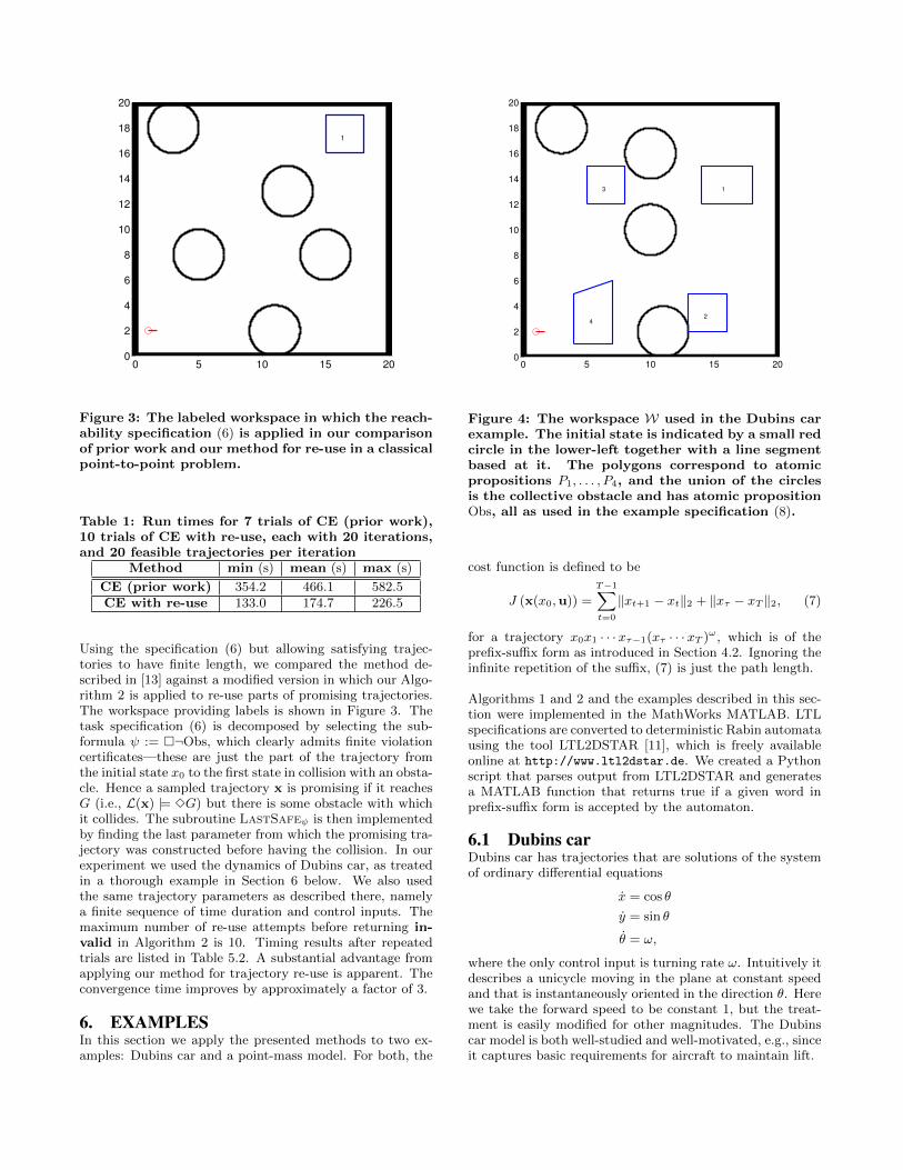
Figure 4: The workspace W used in the Dubins carexample. The initial state is indicated by a small redcircle in the lower-left together with a line segmentbased at it. The polygons correspond to atomicpropositions P1, . . . , P4, and the union of the circlesis the collective obstacle and has atomic propositionObs, all as used in the example specification (8).
cost function is defined to be
J (x(x0,u)) =T�1X
t=0
kxt+1 � xtk2 + kx⌧ � xT k2, (7)
for a trajectory x0x1 · · ·x⌧�1(x⌧ · · ·xT )!, which is of the
prefix-su�x form as introduced in Section 4.2. Ignoring theinfinite repetition of the su�x, (7) is just the path length.
Algorithms 1 and 2 and the examples described in this sec-tion were implemented in the MathWorks MATLAB. LTLspecifications are converted to deterministic Rabin automatausing the tool LTL2DSTAR [11], which is freely availableonline at http://www.ltl2dstar.de. We created a Pythonscript that parses output from LTL2DSTAR and generatesa MATLAB function that returns true if a given word inprefix-su�x form is accepted by the automaton.
6.1 Dubins carDubins car has trajectories that are solutions of the systemof ordinary di↵erential equations
x = cos ✓
y = sin ✓
✓ = !,
where the only control input is turning rate !. Intuitively itdescribes a unicycle moving in the plane at constant speedand that is instantaneously oriented in the direction ✓. Herewe take the forward speed to be constant 1, but the treat-ment is easily modified for other magnitudes. The Dubinscar model is both well-studied and well-motivated, e.g., sinceit captures basic requirements for aircraft to maintain lift.

The labeling function is defined according to the labelingshown in Figure 4, which we call the workspace. Noticethat this defines L only in terms of position (x, y) 2 R2,i.e., labels are independent of orientation. This matches ourintuitive description of tasks in terms of the vehicle visitingor avoiding certain locations. The specification is
⇤W ^⇤¬Obs ^⇤3P1 ^⇤3P2 ^⇤3P3 ^⇤3P4, (8)
where the labeled polygons in the figure have correspond-ing propositions P1, . . . , P4. The union of the circles in thefigure is the obstacle, collectively represented by the atomicproposition Obs. Occupancy of the workspace is enforced by⇤W where the atomic proposition is true only for positionsinside the range [0, 20]⇥ [0, 20].
We parameterize trajectories as sequences of 10 pairs of timedurations and turning rates. The loop index is 5. (Recall theterminology of Section 4.3.) E.g., the first three trajectoryparameter components (one per column)
✓1 1 0.50 ⇡/4 �⇡/4
◆
describe motion that proceeds by steering forward for 1 sec-ond, turning left by ⇡/4 radians (i.e., turning at a rate of⇡/4 radians per second for a total of 1 second), and finallyturning right by ⇡/8 radians.
The sampling distribution is a multivariate Gaussian. Whengenerating samples, we discard those in which the time du-ration is less than zero (because negative input durationsare not meaningful) or the absolute turning rate is greaterthan 1. Because control inputs are bounded, trajectoriesare of bounded curvature, which in addition to the constantforward speed renders the example nontrivial.
Providing some of the details for Line 8 of Algorithm 1 inthis example, sampled trajectories are constructed as fol-lows. First, sample a matrix of durations and turning rates.Then apply it as a piecwise constant steering input. Let x⌧be the state reached after applying the first four parametercomponents (i.e., first four columns of the sampled matrix),and let xT be the state reached after applying all of thesampled inputs. (Recall that p = 5 is the loop index inthis example.) The desired prefix-su�x is finally created bysteering from xT to x⌧ . While our current implementationalways makes this connection by a hard left turn, note thatanalytic solutions for optimal point-to-point steering ignor-ing obstacles is known for Dubins car [15].
Algorithms 1 and 2 were applied for 30 iterations. Exam-ple feasible trajectories found at various times during theoptimization are shown in Figure 5. A plot showing theminimum path length (recall the cost function (7)) trajec-tory found for each iteration is Figure 6. Notice the drasticimprovement following the first few iterations. Such jumpsmay arise from changes in the best homotopy class of trajec-tories found thus far. The plateau of minimum path lengthsbeginning at iteration 21 suggests that a local minimum wasfound.
6.2 Sampling waypointsThe example in this section demonstrates the case of sam-pling waypoints and then using local planners to create a full
0 5 10 15 200
2
4
6
8
10
12
14
16
18
20
1
2
3
4
0 5 10 15 200
2
4
6
8
10
12
14
16
18
20
1
2
3
4
0 5 10 15 200
2
4
6
8
10
12
14
16
18
20
1
2
3
4
Figure 5: Demonstration of the improvement of tra-jectories. From top to bottom, feasible trajectoriesare shown from iterations 1, 15, and 30, respectively.The small line segments drawn along the path indi-cate orientation of Dubins car.

5 10 15 20 25 3038
39
40
41
42
43
44
45
46
47P
ath l
ength
(co
st)
Iteration
Figure 6: For each iteration of Algorithm 1 appliedin the example of Section 6.1, the minimum path-length (cost) among feasible sampled trajectoriesis plotted. Compare with the sampled trajectoriesshown in Figure 5.
trajectory. This is distinct from the previous example be-cause, rather than apply a finite sequence of control inputsand obtain the resulting states, we must solve a collectionof boundary-value problems in order to obtain the trajec-tory. As apparent from Line 8 of Algorithm 1, this is acrucial step, and it has the advantage that manual designof the initial sampling distribution is more intuitive becausethe LTL specification in Problem 1 depends on a labelingfunction defined over states, not control inputs. (Recall thesystem model from Section 2.1.)
The workspace used here is the same as in the previous ex-ample, as shown in Figure 4. The same LTL specification(8) is also used.
We do not declare a particular dynamics (1) here. Instead,the crucial aspect is the manner of constructing trajecto-ries, which proceeds as follows. Samples are obtained froma multivariate gaussian distribution. Each sample is a 2⇥10matrix, where each column corresponds to a position in theworkspace, and the sample as whole is a sequence of 10 way-points. Means of the sampling distribution were initializedto locations selected manually as indicated by bold red as-terisks in the top plot of Figure 7.
The initial state x0 is (1, 2), and the tie index is 3. Forthis example, the tie index has the easy interpretation asthe second waypoint, i.e., the su�x of a trajectory is formedby connecting back to the second waypoint. Trajectories areconstructed by cubic spline interpolation between waypointsand the initial state.
7. CONCLUSIONS AND FUTURE DIREC-TIONS
0 5 10 15 200
2
4
6
8
10
12
14
16
18
20
1
2
3
4
0.0
2
0.0
2
0.020.020.0
2
0.02
0.02
0.0
4
0.04
0.0
4
0.04 0.04
0.06
0.06
0 5 10 15 200
2
4
6
8
10
12
14
16
18
20
1
2
3
4
2
24
Figure 7: Demonstration of the improvement of tra-jectories for the example of Section 6.2. Both plotsare displayed in the workspace from Figure 4, whichis used in both examples. The sampling distributionis multivariate Gaussian, and the means of the distri-bution used in the respective iteration are indicatedin each plot by bold red asterisks. Furthermore thecovariance sublevels are indicated by a iso-curveslike a topographic map. The top plot is from thefirst iteration. One of the feasible trajectories foundis shown as a magenta dashed curve. The bottomplot is from iteration 15, and it also includes a feasi-ble trajectory found at that iteration. The samplingdistribution is very tight and the covariance levelsare mostly occluded.

We presented a stochastic optimization algorithm for opti-mal trajectory generation for nonlinear systems operatingin complex configuration spaces with linear temporal logicspecifications. Importantly, each iteration of our algorithmruns in time polynomial in the size of the system and spec-ification, and does not require the computation of a dis-crete abstraction or automaton. However, it may be ben-eficial to pre-compute an appropriate automaton to practi-cally increase the e�ciency of the algorithm. Additionally,we demonstrated how re-sampling parts of partially infeasi-ble trajectories can result in empirically faster convergencecompared to a state-of-the-art method.
One promising avenue for future work is planning for stochas-tic systems. A chance-constrained approach could take intoaccount disturbances during the planning stage to computea “robust” or “risk- aware” open-loop trajectory. Addition-ally, feedback control policies could be computed by consid-ering a sampling distribution over value functions instead oftrajectories.
Another direction is to generalize the notion of trajectoryreuse. The notion of edit distance between strings, has beenused to compute minimal corrections to strings so that theybelong to a regular language [21]. Similar techniques foromega-regular languages could be used to develop a moreprincipled approach to trajectory reuse in stochastic opti-mization.
We are in the process of performing detailed experimentalcomparisons with similar state-of-the-art methods, e.g., [9].
AcknowledgementsThe authors thank Marin Kobilarov for providing sourcecode implementing the CE method in MATLAB. This workwas partially supported by United Technologies Corpora-tion and IBM, through the industrial cyberphysical systems(iCyPhy) consortium.
8. REFERENCES[1] R. Alur, T. A. Henzinger, G. La↵erriere, and G. J.
Pappas. Discrete abstractions of hybrid systems. Proc.IEEE, 88(7):971–984, 2000.
[2] C. Baier and J.-P. Katoen. Principles of ModelChecking. MIT Press, 2008.
[3] A. Bauer, M. Leucker, and C. Schallhart. Runtimeverification for LTL and TLTL. ACM Trans. Softw.Eng. Methodol, 40(4), September 2011.
[4] C. Belta and L. C. G. J. M. Habets. Controlling of aclass of nonlinear systems on rectangles. IEEE Trans.on Automatic Control, 51:1749–1759, 2006.
[5] A. Bhatia, M. R. Maly, L. E. Kavraki, and M. Y.Vardi. Motion planning with complex goals. IEEERobotics and Automation Magazine, 18:55–64, 2011.
[6] E. M. Clarke and P. Zuliani. Statistical modelchecking for cyber-physical systems. In Proc. ofAutomated Technology for Verification and Analysis,pages 1–12, 2011.
[7] G. E. Fainekos, A. Girard, H. Kress-Gazit, and G. J.Pappas. Temporal logic motion planning for dynamicrobots. Automatica, 45:343–352, 2009.
[8] R. Grosu and S. A. Smolka. Monte Carlo model
checking. In In Proc. of Tools and Algorithms forConstruction and Analysis of Systems, pages 271–286,2005.
[9] S. Karaman and E. Frazzoli. Sampling-basedalgorithms for optimal motion planning withdeterministic µ-calculus specifications. In Proc. ofAmerican Control Conf., 2012.
[10] S. Karaman, R. G. Sanfelice, and E. Frazzoli. Optimalcontrol of mixed logical dynamical systems with lineartemporal logic specifications. In Proc. of IEEE Conf.on Decision and Control, pages 2117–2122, 2008.
[11] J. Klein and C. Baier. Experiments with deterministic!-automata for formulas of linear temporal logic.Theoretical Computer Science, 363:182–195, 2006.
[12] M. Kloetzer and C. Belta. A fully automatedframework for control of linear systems from temporallogic specifications. IEEE Trans. on AutomaticControl, 53(1):287–297, 2008.
[13] M. Kobilarov. Cross-entropy motion planning. Int. J.of Robotics Research, 31:855–871, 2012.
[14] Y. Kwon and G. Agha. LTLC: Linear temporal logicfor control. In Proc. of HSCC, pages 316–329, 2008.
[15] S. M. LaValle. Planning Algorithms. Cambridge Univ.Press, 2006.
[16] N. Markey and P. Schnoebelen. Model checking apath. In Proc. of the Int. Conf. on ConcurrencyTheory, 2003.
[17] T. Nghiem, S. Sankaranarayanan, G. Fainekos,F. Ivancic, A. Gupta, and G. J. Pappas. Monte-Carlotechniques for falsification of temporal properties ofnon-linear hybrid systems. In Proc. of the 13th ACMInternational Conference on Hybrid Systems:Computation and Control, pages 211–220, 2010.
[18] E. Plaku. Planning in discrete and continuous spaces:from LTL tasks to robot motions. In Advances inAutonomous Robotics. Springer, 2012.
[19] R. Y. Rubinstein and D. P. Kroese. The Cross-entropyMethod: A Unified Approach to CombinatorialOptimization. Springer, 2004.
[20] S. Sankaranarayanan and G. Fainekos. Falsification oftemporal properties of hybrid systems using thecross-entropy method. In Proc. of the 15th ACMInternational Conference on Hybrid Systems:Computation and Control, pages 125–134, 2012.
[21] R. A. Wagner. Order-n correction for regularlanguages. Commun. ACM, 17(5):265–268, 1974.
[22] E. M. Wol↵ and R. M. Murray. Optimal control ofnonlinear systems with temporal logic specifications.In Proc. of Int. Symposium on Robotics Research,2013.
[23] E. M. Wol↵, U. Topcu, and R. M. Murray.Optimization-based control of nonlinear systems withlinear temporal logic specifications. In Proc. of Int.Conf. on Robotics and Automation, 2014.
[24] T. Wongpiromsarn, U. Topcu, and R. M. Murray.Receding horizon temporal logic planning. IEEETrans. on Automatic Control, 2012.
[25] H. L. S. Younes and R. G. Simmons. Probabilisticverification of discrete event systems using acceptancesampling. In In Proc. 14th International Conferenceon Computer Aided Verification, pages 223–235, 2002.