Embed Size (px)
Citation preview

Crop water parameters of irrigated wine and table grapes tosupport water productivity analysis in the Sao Francisco riverbasin, Brazil
A.H. de C. Teixeira a,b,*, W.G.M. Bastiaanssen c,d, L.H. Bassoi a
aEmbrapa Semi-Arido, P.O. Box 23, 56302-970 Petrolina, PE, BrazilbWageningen University and Research Centre, Centre for Water and Climate, Droevendaalsesteeg 4,
6708 PB Wageningen, The NetherlandscWaterWatch, Generaal Foulkesweg 28, 6703 BS Wageningen, The NetherlandsdDelft University of Technology, Stevinweg 1, 2600 GA Delft, The Netherlands
a g r i c u l t u r a l w a t e r m a n a g e m e n t 9 4 ( 2 0 0 7 ) 3 1 – 4 2
avai lab le at www.sc iencedi rec t .com
journal homepage: www.e lsev ier .com/ locate /agwat
a r t i c l e i n f o
Article history:
Received 26 January 2007
Accepted 9 August 2007
Published on line 14 September 2007
Keywords:
Vitis vinifera L.
Energy balance
Evapotranspiration
Crop coefficient
Water productivity
Bowen ratio
Evaporative fraction
a b s t r a c t
Energy and water balance parameters were measured in two commercial vineyards in the
semiarid region of the Sao Francisco river basin, Brazil. Actual evapotranspiration (ET) was
acquired with the Bowen ratio surface energy balance method. The ratio of the latent heat
flux to the available energy, or evaporative fraction (EF), was 81% on average for two growing
cycles in wine grape and 88% for two growing seasons in table grape. Energy partitioning in
this last vineyard was higher due to microsprinkler irrigation conditions and greater soil
cover promoted by the overhead horizontal trellis systems. The accumulated ET from
pruning to harvest in wine grape was 438 and 517 mm for the first and second growing
cycles, respectively. Table grape consumed less water than wine grape (393 and 352 mm for
the first and second growing seasons, respectively) due to shorter crop stages. Beneficial
transpiration (T) was 89 and 81% of total ET for wine and table grape, respectively. Brazilian
semiarid climate allows 2.5 production cycles per year for vineyards. The yield was in
average of 6183 kg ha�1 for two cycles of wine grape and 11,200 kg ha�1 for one short growing
season of table grape, corresponding to a bio-physical water productivity per unit ET of
1.06 kg m�3 (or 1.02 L wine m�3) and 3.18 kg m�3, respectively. Table grape showed a sig-
nificantly higher economic water productivity (US$ 6.51 m�3) than wine grape (US$
0.93 m�3). These values are much favorable than for staple crops.
# 2007 Elsevier B.V. All rights reserved.
1. Introduction
Irrigated crops in the semiarid region of Sao Francisco river
basin in Brazil consist mainly of fruit crops, such as grapes,
mangos, bananas and guavas. The average rainfall in this region
is 570 mm year�1, and the rainy period is concentrated from
January to April. The reference evapotranspiration (ETo) is
around 1600 mm year�1. The monthly average air temperature
varies between 24 and 30 8C only. Under such high evaporative
* Corresponding author at: Embrapa Semi-Arido, P.O. Box 23, 56302-97E-mail addresses: [email protected], heriberto.teixeira@
0378-3774/$ – see front matter # 2007 Elsevier B.V. All rights reservedoi:10.1016/j.agwat.2007.08.001
atmospheric demand and low and irregular rainfall, irrigation
becomes necessary for commercial agriculture.
The vineyards growing under these permanently warm
conditions exhibit an agronomic behaviour being different
from the temperate climates. While in these last climates, a
typical winter season induces dormancy in grapes, the
continuous physiological processes in the semiarid region of
Brazil are accelerated and the propagation is very fast allowing
the first production after 1.5 years.
0 Petrolina, PE, Brazil. Tel.: +55 87 38621711; fax: +55 87 38621744.wur.nl (A.H. de C. Teixeira).
d.

a g r i c u l t u r a l w a t e r m a n a g e m e n t 9 4 ( 2 0 0 7 ) 3 1 – 4 232
With proper irrigation and cultural management practices,
the farmers in Sao Francisco valley can produce grapes and
wine in any time of the year, allowing on average 2.5
production cycles per year and the harvests in periods with
higher prices, although for seedless table grapes, the rainy
period is avoided due to the direct damage to the fruits and the
high occurrence of diseases.
Crop water productivity (CPW) – or its equivalent water use
efficiency for irrigated crops – represents the fresh fruit or
wine production per unit of water applied or consumed. It is
preferred to analyse CPW in terms of consumptive use
because it includes also non-irrigation sources of water, such
as rainfall, seepage and soil moisture changes.
The amount of applied water is partitioned into evapo-
transpiration and deep percolation. Actual evapotranspiration
(ET) represents the water that is vapourized and not longer
available to downstream users of a river basin. Percolated
water can be recycled, and should therefore not be ascribed to
the production of a certain irrigated crop.
The term ‘‘water productivity’’ reflects the link between
production of an intended good and its resource input (Molden
and Satkhivadivel, 1999; Kijne et al., 2003; Bos et al., 2005;
Molden et al., 2007), having a more general basis than the term
‘‘water use efficiency’’, and makes it suitable to compare the
economic performance with other water use sectors.
It is deemed necessary to study the energy and water
balances of vineyards for understanding and predicting CPW
(Bastiaanssen et al., in press). As wine and table grapes are
cultivated in different trellis and irrigation systems in the Sao
Francisco river basin, it is important to quantify various grape
water parameters under these differences, being ET the most
important of them.
ET from vineyards can be obtained accurately using
weighing lysimeters (Evans et al., 1993; Williams et al., 2003;
Williams and Ayars, 2005b), eddy correlation techniques (Oliver
and Sene, 1992; Sene, 1994; Trambouze et al., 1998; Ortega-
Farias et al., 2007) and the Bowen ratio energy balance method
(Heilman et al., 1994, 1996; Rana et al., 2004; Yunusa et al., 2004).
These studies reveal a significant variation in water
consumption due to different irrigation strategies and cultural
practices. While certain farmers prefer the production of high
quantities of berries, others like a high quality product
introducing significant water stress levels by partial root zone
drying and deficit irrigation.
The extrapolation of field measurements to irrigation
schemes, regions and river basins are, therefore, cumbersome
(Williams and Ayars, 2005b). With simultaneous measure-
ments of ET and ETo, it is possible to determine the crop
coefficient (kc) that normalizes ET for climatic influences. This
coefficient reflects the canopy development and vineyard
water status as the crop stages progress (Snyder et al., 1989).
As Brazil is a developing country on fast track with a growing
export of fresh fruits and wines, on-farm water management in
vineyards is the cornerstone for a productive use of scarcewater
resources at the basin scale. The objective of this study was the
determination of water parameters related to ET such as crop
coefficients, evaporative fraction, soil evaporation and canopy
transpiration, bulk surface and canopy resistances and crop
water productivity for wine and table grapes growing under
different trellis and irrigation systems. Upscaling of these data
sets is a good bio-physical basis for appraising the options for
increasing total CPW at the regional scale.
2. Vineyards investigated
2.1. Wine grapes with drip irrigation and vertical trellis
The wine grape investigated stands at Vitivinıcola Santa Maria
farm near the town of Lagoa Grande in Pernambuco state
(latitude 098020S; longitude 408110W). The cultivar is Petite
Syrah, and the vineyard was 11 years old during the field
investigation in 2002.
The plants are spaced at 1.20 m � 3.50 m, trained vertically
to a bilateral cordon and spur pruned. The cordon wire was at a
height of 1.6 m with no foliage wires (a sprawl type canopy
developed). There was no cover crop between the rows, and
they are oriented in a north–south direction. The shoots are
allowed to grow freely over the wires. Vertical trellis systems
in wine grape are preferred instead the overhead horizontal
because it makes easier the mechanical practices.
The daily drip irrigated area of 4.13 ha was bordered on all
sides by other wine grapes. There was one drip emitter
between two plants in the rows at a discharge rate of 4 L h�1,
suspended on the wire. Although it is common in many wine
production areas not to irrigate vines at budbreak, or shortly
thereafter, the irrigation manager started the irrigation soon
after pruning with a fixed and large amount of water without
quantifying the water demand.
The soil is sandy with a water retention capacity that
increases with depth, presenting a cracked rock layer below
0.60 m evidenced by the time of installing the tensiometers.
Because the vineyard was pruned two times in 2002, the
study involved two growing cycles during this year. The
duration of the first growing cycle (GC1) was 132 days, elapsing
from 7 February to 19 June 2002, while the second growing
cycle (GC2) comprised 136 days, from 8 July to 22 November
2002. Grapes were picked to produce wine from both periods.
The Bowen ratio surface energy balance method was used to
measure the partition of net available energy into sensible and
latent heatfluxes.The sensorswere installed at the centre of the
plot. The gradients of air temperature and vapour pressure
above the crop were calculated by using wet and dry thermo-
couplesofcupper/constantanat0.5and1.5 mabovethecanopy.
The surface albedo (a = RR/RG) was measured through
incident (RG) and reflected (RR) global solar radiation acquired
with pyranometers faced up and down (model Eppley, Rhod
Island, USA). The net radiation (Rn) was measured at 1 m over
the canopy with two net radiometers (model NR-Lite, Kipp &
Zonnen, Delft, The Netherlands), each one installed above a
row of plants.
The soil heat flux (G) was obtained with four heat flux plates
(HFT3-L, REBS, Radiation and Energy Balance Systems, Seattle,
WA and Hukseflux, Delft, The Netherlands) at 0.02 m soil depth
and 0.50 m from the plants. Two plates were burried at the west
and the other two at the east side of two rows of plants.
Wind speed was measured with anemometers (03101, R.M.,
Young wind Sentry, Michigan, USA) at two levels, i.e. 1.0 and
2.0 m above the canopy. Air temperature and relative
humidity at 0.5 m above the canopy were obtained with a

a g r i c u l t u r a l w a t e r m a n a g e m e n t 9 4 ( 2 0 0 7 ) 3 1 – 4 2 33
probe from Vaisala (model HMP 35A, Helsinki, Finland), inside
the shelter at the first level of the thermocouples.
Soil moisture profiles were weekly monitored with tensi-
ometers located between the drip emitters and the vine
trunks. The sampling depths were 0.2, 0.4 and 0.6 m
considered to represent the effective root zone for vineyards
in local soil and cultural conditions (Bassoi et al., 2003).
Tensions were converted into soil moisture by using labora-
tory measurements of soil water retention curves. Applied
water by irrigation was obtained by simple weekly readings of
water meters attached to the drip pipes.
2.2. Table grapes with microsprinkler irrigation andoverhead horizontal trellis
The table grape plot is located at Vale das Uvas farm near the
town of Petrolina, Pernambuco state (latitude 098180S; longitude
408220W). The cultivar is the Superior Seedless and the vineyard
was only 2 years old at the start of the measurement campaign.
The plants are spaced at 3.5 m � 4.0 m, with the rows
oriented in the usual north–south direction. The vineyard has
an overhead horizontal trellis system at 1.80 m height. The
cover crop consists of a mixture of legumes and grasses, and
was incorporated into the soil after budbreak.
The plot investigated is 5.13 ha, surrounded by other table
grapes. The grapes were daily microsprinkler irrigated, with
one in-line microsprinkler between two vines on the ground at
a discharge rate of 44 L h�1 which wetted 70% of the soil
surface. As in wine grape, the farmer started the irrigation
soon after pruning with large amount of water, thereby
promoting high rates of direct soil evaporation and cover crop
transpiration at initial stages.
The soil is also sandy throughout the vertical profile, but its
water retention capacity does not increase with depth. Water
holding capacity is higher in the upper soil layer (0–20 cm) due
to high organic matter content.
The measurements involved two growing seasons (GS1 and
GS2), during the same period but in different years: both from 8
July to 7 October, in 2002 and in 2003. The duration of the
growing seasons were 90 days only, being extremely short as
compared to vineyards in California and Australia among
others. The grapes were brought to the export market at the
end of GS2 in 2003.
The crop was left resting between the two seasons to avoid
possible direct damage in fruits and high incidence of fungi
diseases due to rainfall. The plants were not girdled nor
sprayed with gibberellic acid and the leaves were not removed
from fruit zone. At the stage of vegetative growth, non-fruitful
shoots and lateral shoots growing in the fruiting zone were
removed and at fruit growth stage, the berries were protected
with a white cover from direct solar radiation.
The same method, measurement procedures and equip-
ment’s manufacturers as for wine grapes were set up for table
grapes with few differences. Two net radiometers were
installed, with one instrument at 1 m over the canopy and
the other at 1 m above the ground surface to measure
intercepted radiation by the canopy. Two heat flux plates
(model HFT3-L, REBS, Radiation and Energy Balance Systems,
Seattle, WA) were used, one at the east and the other at the
west side of two rows of plants.
Air temperature and relative humidity near the leaves was
measured by a probe (SKH 2013, Sky instruments LTD,
Llandrindod Wells, UK) installed in the arm of the datalogger’s
shelter at 0.5 m bellow the trellis system and only one level
anemometer was installed at 1.0 m above the canopy.
Soil moisture profiles and applied water by irrigation were
weekly monitored with tensiometers located between the
emitters and the vine trunks along two rows at same soil
depths as for wine grapes and with water meters in
microsprinkler pipes.
3. Methodology
The energy balance equation of a vineyard can be expressed by
means of bulk energy and heat fluxes:
Rn � lEv � G� Hv ¼ 0 (1)
where Rn is the net radiation, lEv the latent heat flux from the
vineyard, Hv the sensible heat flux from the vineyard and G is
the soil heat flux. lEv was obtained by a partitioning parameter:
lEv ¼Rn � G1þ b
(2)
where b is the Bowen ratio:
b ¼ gDTDe
� �(3)
and g (kPa 8C�1) is the psychrometric constant, DT (8C) the
temperature gradient measured by the dry thermocouples
and De (kPa) is the vapour pressure gradient measured by
the difference between dry and wet thermocouples over the
height interval above the canopy surface.
The actual evapotranspiration (ET) was derived from the
latent heat of vaporization (l), density of water and lEv. As a
first approximation, an ET of 1 mm day�1 is equivalent to lEv
of 28 W m�2. With measured values of Rn and G and
estimations of lEv, the sensible heat flux from the vineyards
(Hv) was obtained as a residual in Eq. (1).
The ETo was calculated in this study following FAO-56
standardized guidelines (Allen et al., 1998), using weather data
from an automatic agrometeorological station near the table
grape plot (at a distance of 200 m), also equipped with a
pluviometer to measure rainfall. The crop coefficient (Kc) was
obtained as ET/ETo. For the further separation of ET into
transpiration (T) and soil evaporation (E), the dual crop
coefficient approach of FAO-56 was used with the basal crop
coefficients (Kcb) and soil evaporation coefficients Ke
(Ke = Kc � Kcb):
T ¼ KcbETo (4)
E ¼ KeETo (5)
Initial and end values of Kcb were derived from the values at
the lower envelope of daily measured Kc at these stages when
foliage development is minimal. The mid-stage Kcb values

a g r i c u l t u r a l w a t e r m a n a g e m e n t 9 4 ( 2 0 0 7 ) 3 1 – 4 234
have been taken from Allen et al. (1998). Tabulated values for
mid-stage Kcb are 0.80 for table grape and 0.65 for wine grape
which were adjusted for the our specific weather conditions:
Kcb ¼ KcbðtabularÞ þ f0:04ðu2 � 2Þ � 0:004ðRHmin
� 45Þg hv
3
� �0:3
(6)
where u2 and RHmin are, respectively, the averaged wind speed
and minimum relative humidity at the agrometeorological
station (at a height of 2 m) and hv (m) is the mean plant height
for the mid-stage periods.
One key parameter in ET processes is the aerodynamic
resistance (ra) that describes the turbulence of the atmo-
sphere, and is related to the roughness of the land surface. The
surface roughness parameters of the vineyards were esti-
mated from the flux profile relationships.
The atmospheric surface-layer similarity theory was used
(Stull, 1988; Monteith and Unsworth, 1990) applying universal
integrated stability functions of temperature (Ch) and momen-
tum (Cm) for relating fluxes to atmospheric state profiles and
surface properties (Businger et al., 1971).
The friction velocity, u* (m s�1), which is a velocity scale
related to mechanically generated turbulence, was calculated
from two-level (z1, z2) wind speed measurements (u1, u2):
u� ¼kðu2 � u1Þ
ln½ðz2 � dÞ=ðz1 � dÞ� � cmððz2 � dÞ=LÞ þ cmððz1 � dÞ=LÞ (7)
The aerodynamic resistance, ra (s m�1), between the
surface roughness and the canopy level from where atmo-
spheric state variables are measured was calculated as:
ra ¼ln½ðz1 � dÞ=z0h�
ku�� ch (8)
The surface roughness length for moment transfer (z0m)
that together the roughness length for heat and vapour
transfer (z0h = 0.1 z0m) controls u* and ra was obtained from:
z0m ¼z1 � d
expððku1=u�Þ þ CmÞ(9)
In Eqs. (7)–(9), u1 and u2 are the wind speed values at heights
z1 and z2 (2.6 and 3.6 m for wine grapes and 2.8 and 3.8 m for
table grapes), d is the zero plane displacement height (2/3 of
the mean canopy height), k is the von Karman’s constant (0.41)
and L is the Obukhov length, which was obtained by an
iterative numerical method starting with a value of 106 m.
The wind speed in table grapes was measured only at 2.8 m.
The values at 3.8 m, necessary for solving u* in Eq. (7), were
estimated by means of Hv and field measurements of DT
considering initially neutral conditions solving ra in the
following equation:
Hv ¼ racpDTra
(10)
where ra and cp are the air density and air specific heat at
constant pressure.
The first values for u* were then calculated by Eq. (8) using
the height levels of 3.8 and 2.8 m. The resulted values of u*
were used in Eq. (7) to obtain the wind speed at 3.8 m (u2).
These calculations were performed first without using the
stability correction terms Ch and Cm.
The latent heat flux from the canopy (lEc) was acquired from
transpiration fluxes (T). The continuous measurement of net
radiation over and under the canopy made it possible to obtain
the energy available to the soil surface (Rns) for table grape, as
well to derive the amount absorbed by the canopy
(Rnc = Rn � Rns). With known values of lEv, lEc and ra, the bulk
surface (rs) and canopy (rc) resistances were estimated inverting
the general Penman–Monteith equation (Farah, 2001):
lEv;c ¼saðAEÞ þ racpðVPDÞ=ra
sa þ gð1þ ðrs;cÞ=raÞ(11)
where lEv,c is the latent heat flux from the vineyard (subscript
‘v’) or from the canopy (subscript ‘c’); sa (kPa 8C�1) is the slope
of the saturated vapour pressure curve, AE is the available
energy ((Rn � G) or (Rn – Rns)), ra (kg m�3) is the moist air den-
sity, cp (J kg�1 K�1) is the air specific heat at constant pressure,
VPD (kPa) is the vapour pressure deficit and g (kPa 8C�1) is the
psychrometric constant and rs,c (s m�1) is the bulk surface
(subscript ‘s’) or canopy (subscript ‘c’) resistance to water
vapour transport.
The leaf area index (LAI) was derived for table grape with
the values of intercepted radiation (Teixeira and Lima Filho,
1997) and consideration of the inversion of Beer’s law:
LAI ¼ 0:17� 1:24 lnRns
Rn
� �(12)
Crop water productivity (CWP) is commonly expressed in
yield per unit of applied water, including rainfall and irrigation
(Peacock et al., 1977; Araujo et al., 1995; Srinivas et al., 1999). In
this study, it was calculated as:
CWPET;T;IRR ¼Yact
WET;T;IRR(13)
where the subscripts ET and T denote the water fluxes by
evapotranspiration and transpiration, respectively; the sub-
script IRR denote the amount of water supplied by irrigation
andYact is the actual yield of wine or fruits. Following Droogers
et al. (2000) and Bos et al. (2005), the economic indicators used
were the standard gross value of production (wine and grapes)
over the irrigation supply (CPW$_IRR) and over evapotranspira-
tion (CPW$_ET) and transpiration (CPW$_T).
4. Results and discussion
4.1. Soil moisture and weather conditions
The values of soil moisture (SM) are shown in Fig. 1. SM at
20 cm depth showed more variations with time, than at deeper
soil layers in both vineyards. This is an expected result
because of the dynamics of infiltration and subsequent
depletion by root water uptake and soil evaporation.

Fig. 1 – Soil moisture (SM) at different depths (20, 40 and 60 cm), during the growing cycles of 2002 of wine grape and for the
growing seasons of 2002 and 2003 of table grape.
a g r i c u l t u r a l w a t e r m a n a g e m e n t 9 4 ( 2 0 0 7 ) 3 1 – 4 2 35
The maximum values of SM in the wine grape were found
at 60 cm depth pinpointing that moisture assembles in the
lower root zone and is not easily drained away. This could be
related to the increasing retention properties and reduced
permeability at this soil depth. For table grape, the values are
over against that maximal at 20 cm, which reveals typical free
drainage conditions. SM varied during most days between 0.19
and 0.29 cm3 cm�3 in both vineyards, which is similar to the
range those from Ortega-Farias et al. (2007) in Chile.
A regular soil moisture trend line reflects a constant supply
and removal of irrigation water. Water excess can arise if
supply exceeds removal by root water uptake, what in wine
grape, could adversely affect the production and quality of
wine. This excess not only enhances the loss of scarce water
resources but also valuable nutrients can be leached out from
the root zone.
July and October are the coldest and the warmest months
of the year, respectively. The difference between the values of
air temperature (Ta) near the canopies and at the routine
agrometeorological station was small (see Fig. 2a and b). The
seasonal average near-canopy Ta in wine grape was with
26.5 8C, slightly higher than the 25.2 8C for table grape. The
lower values in the last vineyard can be ascribed to the higher
soil cover caused by the overhead trellis system and micro-
sprinkler irrigation.
The higher values of wind speed (W) in the study region
normally happen during the driest period, between August
and October, with longer term values reaching 3.0 m s�1 in
September. The lowest values occur during the rainy period
with monthly average of 1.6 m s�1. The daily variations of W
over the vineyards and at agrometeorological station are
depicted in Fig. 2c and d. During 2002 and 2003, averaged daily
values were above 0.8 m s�1 and lower than 3.0 m s�1 for both
vineyards. The above-canopy wind speed measurements
accounted for 80% of those from the station, which can be
ascribed to differences in surface roughness.
The high values of Ta together with the dryness of the air
induce high vapour pressure deficit (VPD) conditions outside
the rainy period. The monthly averaged relative humidity in
the region ranges from 55 to 70%. The 24 h averaged values of
VPD for the study period are plotted in Fig. 2e and f. Moister air
near the canopy can be attributed to irrigation that raises the
air humidity. This effect was greater in microsprinkler
irrigation system of table grape than for the drip irrigation
in wine grape.
According to Fig. 2g and h, global solar radiation (RG)
decreased in the first half of the year of 2002 and increased
during the second halves of the years 2002 and 2003. ETo
followed RG. Higher values of RG in the second half of 2002
established a slightly higher value for Ta and ETo, in
comparison with the same period in 2003. ETo was 4.4 and
5.0 mm day�1 on average for the first and second halves of
2002, while it was 4.1 mm day�1 during the second half of
2003. The total rainfall during the first half of 2002 was
41.4 mm, and in the second half of the same year, it was
49.3 mm. It rained only 17.3 mm during the growing season of
table grape in 2003.
4.2. Energy partitioning
The values of the components of the energy balances – and
the latent heat flux from the vineyard (lEv) in particular –
varied according to RG. The diurnal variation of these
components for the period of measurements is depicted in
Fig. 3. Maximum midday lEv were around 400–500 W m�2 for
both vineyards.
The fluxes had a very smooth behaviour during daytime
hours, with an exception for G in wine grape, which presented

Fig. 2 – Daily values of weather variables during the study period in 2002 and 2003 from agrometeorological station (station)
and near the canopies of wine grape (wine) and table grape (table): (a and b) mean air temperature (Ta); (c and d) wind speed
(W); (e and f) vapour pressure deficit (VPD); (g and h) incident global solar radiation (RG), reference evapotranspiration (ETo)
and rainfall.
a g r i c u l t u r a l w a t e r m a n a g e m e n t 9 4 ( 2 0 0 7 ) 3 1 – 4 236
midmorning and midafternoon peaks and lower values at
midday due to the canopy architecture, what is in agreement
with Heilman et al. (1994).
Daily averages of energy balances components for
wine grape in 2002 are presented in Table 1. Rn was on
average 46% of RG for both growing cycles. A fraction
of approximately 50% is in agreement with earlier crop
science radiation studies (e.g. Makkink, 1957; Oliver and
Sene, 1992).
The sensible heat flux from the vineyard (Hv) accounted
for 18% of Rn for both growing cycles of wine grape, being
a modest heat flux. During the first cycle, the daily averaged
G was negative because heat was released from the
warm soil body. The opposite situation occurred during
the second cycle. The largest portion of Rn was converted
into lEv, which represented around 83 and 78% of Rn in
the first and second growing cycles, respectively, corre-
sponding to an evaporative fraction (EF = lEv/(Rn � G))
around 81%.
Daily averages of energy balance components for table
grape in 2002 and 2003 are presented in Table 2. Rn represented
a fraction of 55% of RG, being higher than for wine grape; the
overhead trellis and microsprinkler irrigation system promote
lower both, albedo and longwave emission, increasing Rn. The
measured albedo in wine grape in the actual study varied
between 0.19 and 0.24. These values are higher than for
microsprinkler irrigated table grape (0.18–0.23) reported by
Azevedo et al. (1997).
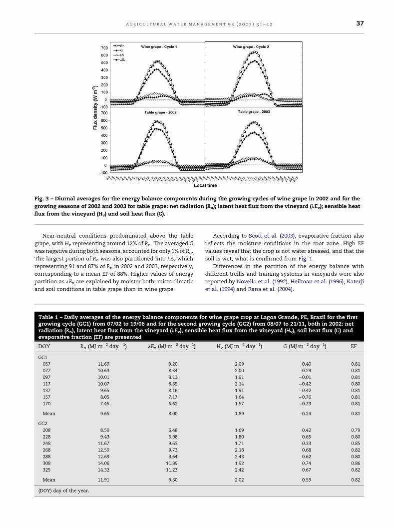
Fig. 3 – Diurnal averages for the energy balance components during the growing cycles of wine grape in 2002 and for the
growing seasons of 2002 and 2003 for table grape: net radiation (Rn); latent heat flux from the vineyard (lEv); sensible heat
flux from the vineyard (Hv) and soil heat flux (G).
a g r i c u l t u r a l w a t e r m a n a g e m e n t 9 4 ( 2 0 0 7 ) 3 1 – 4 2 37
Near-neutral conditions predominated above the table
grape, with Hv representing around 12% of Rn. The averaged G
was negative during both seasons, accounted for only 1% of Rn.
The largest portion of Rn was also partitioned into lEv which
representing 91 and 87% of Rn in 2002 and 2003, respectively,
corresponding to a mean EF of 88%. Higher values of energy
partition as lEv are explained by moister both, microclimatic
and soil conditions in table grape than in wine grape.
Table 1 – Daily averages of the energy balance components fogrowing cycle (GC1) from 07/02 to 19/06 and for the second grradiation (Rn), latent heat flux from the vineyard (lEv), sensiblevaporative fraction (EF) are presented
DOY Rn (MJ m�2 day �1) lEv (MJ m�2 day�1)
GC1
057 11.69 9.20
077 10.63 8.34
097 10.01 8.13
117 10.07 8.35
137 9.65 8.16
157 8.05 7.17
170 7.45 6.62
Mean 9.65 8.00
GC2
208 8.59 6.48
228 9.43 6.98
248 11.67 9.63
268 12.59 9.73
288 12.69 9.64
308 14.06 11.39
325 14.32 11.23
Mean 11.91 9.30
(DOY) day of the year.
According to Scott et al. (2003), evaporative fraction also
reflects the moisture conditions in the root zone. High EF
values reveal that the crop is not water stressed, and that the
soil is wet, what is confirmed from Fig. 1.
Differences in the partition of the energy balance with
different trellis and training systems in vineyards were also
reported by Novello et al. (1992), Heilman et al. (1996), Katerji
et al. (1994) and Rana et al. (2004).
r wine grape crop at Lagoa Grande, PE, Brazil for the firstowing cycle (GC2) from 08/07 to 21/11, both in 2002: nete heat flux from the vineyard (Hv), soil heat flux (G) and
Hv (MJ m�2 day�1) G (MJ m�2 day�1) EF
2.09 0.40 0.81
2.00 0.29 0.81
1.91 �0.01 0.81
2.14 �0.42 0.80
1.91 �0.42 0.81
1.64 �0.76 0.81
1.57 �0.73 0.81
1.89 �0.24 0.81
1.69 0.42 0.79
1.80 0.65 0.80
1.71 0.33 0.85
2.18 0.68 0.82
2.43 0.62 0.80
1.92 0.74 0.86
2.42 0.67 0.82
2.02 0.59 0.82
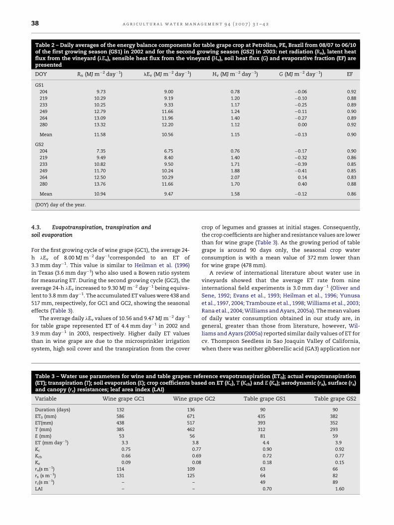
Table 2 – Daily averages of the energy balance components for table grape crop at Petrolina, PE, Brazil from 08/07 to 06/10of the first growing season (GS1) in 2002 and for the second growing season (GS2) in 2003: net radiation (Rn), latent heatflux from the vineyard (lEv), sensible heat flux from the vineyard (Hv), soil heat flux (G) and evaporative fraction (EF) arepresented
DOY Rn (MJ m�2 day�1) lEv (MJ m�2 day�1) Hv (MJ m�2 day�1) G (MJ m�2 day�1) EF
GS1
204 9.73 9.00 0.78 �0.06 0.92
219 10.29 9.19 1.20 �0.10 0.88
233 10.25 9.33 1.17 �0.25 0.89
249 12.79 11.66 1.24 �0.11 0.90
264 13.09 11.96 1.40 �0.27 0.89
280 13.32 12.20 1.12 0.00 0.92
Mean 11.58 10.56 1.15 �0.13 0.90
GS2
204 7.35 6.75 0.76 �0.17 0.90
219 9.49 8.40 1.40 �0.32 0.86
233 10.82 9.50 1.71 �0.39 0.85
249 11.70 10.24 1.88 �0.41 0.85
264 12.50 10.29 2.07 0.14 0.83
280 13.76 11.66 1.70 0.40 0.88
Mean 10.94 9.47 1.58 �0.12 0.86
(DOY) day of the year.
a g r i c u l t u r a l w a t e r m a n a g e m e n t 9 4 ( 2 0 0 7 ) 3 1 – 4 238
4.3. Evapotranspiration, transpiration andsoil evaporation
For the first growing cycle of wine grape (GC1), the average 24-
h lEv of 8.00 MJ m�2 day�1corresponded to an ET of
3.3 mm day�1. This value is similar to Heilman et al. (1996)
in Texas (3.6 mm day�1) who also used a Bowen ratio system
for measuring ET. During the second growing cycle (GC2), the
average 24-h lEv increased to 9.30 MJ m�2 day�1 being equiva-
lent to 3.8 mm day�1. The accumulated ET values were 438 and
517 mm, respectively, for GC1 and GC2, showing the seasonal
effects (Table 3).
The average daily lEv values of 10.56 and 9.47 MJ m�2 day�1
for table grape represented ET of 4.4 mm day�1 in 2002 and
3.9 mm day�1 in 2003, respectively. Higher daily ET values
than in wine grape are due to the microsprinkler irrigation
system, high soil cover and the transpiration from the cover
Table 3 – Water use parameters for wine and table grapes: ref(ET); transpiration (T); soil evaporation (E); crop coefficients basand canopy (rc) resistances; leaf area index (LAI)
Variable Wine grape GC1 Wine grap
Duration (days) 132 136
ET0 (mm) 586 671
ET(mm) 438 517
T (mm) 385 462
E (mm) 53 56
ET (mm day�1) 3.3 3.8
Kc 0.75 0.77
Kcb 0.66 0.69
Ke 0.09 0.08
ra(s m�1) 114 109
rs (s m�1) 131 125
rc(s m�1) – –
LAI – –
crop of legumes and grasses at initial stages. Consequently,
the crop coefficients are higher and resistance values are lower
than for wine grape (Table 3). As the growing period of table
grape is around 90 days only, the seasonal crop water
consumption is with a mean value of 372 mm lower than
for wine grape (478 mm).
A review of international literature about water use in
vineyards showed that the average ET rate from nine
international field experiments is 3.0 mm day�1 (Oliver and
Sene, 1992; Evans et al., 1993; Heilman et al., 1996; Yunusa
et al., 1997, 2004; Trambouze et al., 1998; Williams et al., 2003;
Rana et al., 2004; Williams and Ayars, 2005a). The mean values
of daily water consumption obtained in our study are, in
general, greater than those from literature, however, Wil-
liams and Ayars (2005a) reported similar daily values of ET for
cv. Thompson Seedless in Sao Joaquin Valley of California,
when there was neither gibberellic acid (GA3) application nor
erence evapotranspiration (ET0); actual evapotranspirationed on ET (Kc), T (Kcb) and E (Ke); aerodynamic (ra), surface (rs)
e GC2 Table grape GS1 Table grape GS2
90 90
435 382
393 352
312 293
81 59
4.4 3.9
0.90 0.92
0.72 0.77
0.18 0.15
63 66
64 82
49 89
0.70 1.60

Fig. 4 – Seasonal variation of crop coefficients in vineyards during the growing cycles of 2002 of wine grape and for the
growing seasons of table grape in 2002 and 2003: crop coefficients based on evapotranspiration (Kc), transpiration (Kcb) and
soil evaporation (Ke).
a g r i c u l t u r a l w a t e r m a n a g e m e n t 9 4 ( 2 0 0 7 ) 3 1 – 4 2 39
trunk girdling, comparing with our 3-years-old Superior
Seedless.
On the other hand, as the growing seasons in our study area
are shorter, the seasonal water consumption is lower. A recent
water balance study in vineyards in South Africa (Roux, 2007)
showed that the average value of seasonal ET for wine grape is
621 mm and for table grape is in the range from 519 to 827 mm.
The length of the growing seasons in South Africa is between 6
and 8 months with only one harvest per year.
Actual evapotranspiration (ET) can be corrected for climatic
influences by normalizing it with ETo, producing the crop
coefficients (Kc). The Kc values can be variable with the crop
properties and stress conditions caused by water deficit and
salinity. Under pristine conditions, maximum values can be
taken, and they are often published in tables (e.g. Snyder et al.,
1989; Consoli et al., 2006).
The behaviour of daily Kc is demonstrated in Fig. 4. Note
that our actual growing conditions also include few non-
pristine environmental circumstances. The Kc values at the
initial and the end stages are highly related to the cover crop
and irrigation. For wine grape, the mean weekly values in the
first growing cycle were in the range from 0.65 to 0.82, while for
the second they were from 0.63 to 0.87. For table grape, the
mean weekly averaged Kc values for both growing seasons
varied between 0.77 and 0.91.
The seasonal trend of crop coefficients Kcb and Ke are also
depicted in Fig. 4. After multiplying these coefficients by ETo,
the transpiration (T) and soil evaporation (E) were obtained.
On average, 89–90% of the total ET was used for T and 10–11%
for E in wine grape. For table grape, 79–83% of ET was used for
T and 17–19% for E (Table 3). Thus, microsprinklers have a
higher portion of non-beneficial evaporation than drip
systems.
4.4. Intercepted radiation, leaf area index and resistances
Data availability of Rn above and under the canopy for table
grape allowed the calculation of intercepted net radiation (Rni)
and the estimation of leaf area index (LAI) for the two growing
seasons following Eq. (12). The mean values of LAI were 0.70
during the first growing season and 1.60 for the second
(Table 3) pinpointing a situation of a young maturing vineyard.
The last value of LAI is close to that found by Rana et al. (2004)
for table grapes in Italy and by Yunusa et al. (2004) for mature
Sultana grapes, growing in a T-trellis system in Australia.
Klaasse et al. (2007) reported LAI values between 2.5 and 3.0
for the table grapes and around 1.0 for wine grapes, in Hex
River Valley, West Cape Province (South Africa). According to
Katerji et al. (1994), LAI for vineyards in rows with a dominant
vertical plant structure present value around 0.70–0.80. There
were no measurements of Rni to allow LAI estimations in wine
grapes in the actual study.
The seasonal variations of aerodynamic resistance (ra) and
the surface (rs) and canopy (rc) resistances are shown in Fig. 5.
Averaged values are found in Table 3. In wine grape, the values
of ra stayed in the range from 78 to 170 s m�1, while for table
grape, the range was from 30 to 160 s m�1. The lower ra values
in the last vineyard can be related to the aerodynamic
smoother horizontal trellis systems. A higher LAI and soil
cover cause a shelter effect (e.g. Verhoef et al., 1997).
The rs values in wine grape were between 35 and 240 s m�1.
For table grape, the range was from 10 to 140 s m�1. Heilman
et al. (1994) found maximum values of rs of 50 and 75 s m�1.
The canopy resistance (rc) for table grape in both years stayed
between 20 and 182 s m�1. Assuming that the stomatal
resistance (rst) can be roughly estimated by (0.5 � LAI � rs)
as reported in several handbooks (Allen et al., 1998), the mean

Fig. 5 – Seasonal trends of calculated aerodynamic (ra), surface (rs) and canopy resistances (rc), during the growing cycles of
wine grape and for the growing seasons of table grape in 2002 and 2003.
a g r i c u l t u r a l w a t e r m a n a g e m e n t 9 4 ( 2 0 0 7 ) 3 1 – 4 240
values of rst become 22 and 66 s m�1, for the first and second
growing seasons, respectively (Table 3).
Winkel and Rambal (1990) described the stomatal response
of different French vineyards. The minimum rst was 73 s m�1
for Carignane, 93 s m�1 for Merlot and 114 s m�1 for Shiraz.
According to them, the main reason for these differences
could be attributed to different conditions of VPD, soil cover,
soil moisture and evaporative demand. Ben-Asher et al. (2006)
measured recently the rst of grapes under saline irrigation
conditions in Israel, and they showed minimum values of
135 s m�1.
The low values of rs, rc and rst in irrigated vineyards of
semiarid conditions in Brazil are due to wet conditions for
both, soil and air near the canopies. The magnitude of the
differences between rs and rc in table grapes comparing the
two growing seasons can be explained because for the younger
vineyard in 2002, the lower intercepted radiation promoted the
soil component to represent a relative large fraction of rs
(Fig. 5).
The accumulated values of ETo and ET; T and E; together
with the mean values of Kc, Kcb and Ke; ra and rs are shown in
Table 3. For table grape, the averaged values of LAI and rc are
also presented. The different magnitudes of grape water
parameters between the two vineyards are due to differences
in crop stages, age and varieties, trellis and irrigation systems,
soil cover and cultural management.
4.5. Crop water productivity
Only a few studies relate yields of grapes and wine to ET that is
the true consumptive use of vineyards. Organizations
responsible for irrigation management are interested in yield
per unit applied irrigation water (CWPIRR), as it is their duty to
enhance yield through irrigation processes. The drawback is
that not all irrigation water is used for generating crop
production.
Large portion of applied irrigation water turns into
percolation losses (Table 4). The values of percolation were
computed as the differences between rainfall, irrigation and
ET, and there are no corrections made for soil storage changes.
It is worrisome to note that the percolation rates had the same
magnitude as ET.
A summary of all crop water productivity parameters for
both vineyards is presented in Table 4. Wine yield values
(3300–6600 L ha�1) are inside in what is expected to be normal
practices in this region. The differences in yield of bottled wine
between the first (3376 L ha�1) and the second growing cycles
(6514 L ha�1) pinpoint seasonal effects. The first cycle was
cloudier and duration of the days during the stages of flower
and maturation of fruits were shorter than the in the second
cycle.
Although the productivity for one cycle of wine grape is
lower than in regions where the climate is temperate, the total
production of two cycles in 1 year is in good agreement with
for instance South Africa (Roux, 2007). Whereas the first cycle
yielded an economical water productivity of 0.35, 0.70 and US$
0.80 m�3 based on irrigation, ET and T, respectively, these
values for the second growing cycle increased to US$ 0.62, US$
1.15 and US$ 1.28 m�3.
The yield in 2002 for table grape was not marketable. Only
the growing season in 2003 was analyzed for productivity
purposes. The yield of fresh table grapes (11,200 kg ha�1) is in
agreement with the public perception in the Sao Francisco
river basin. At a double cycle, the yield could increase to
22.4 tonnes ha�1. The CWPET values for marketable table grape
(3.18 kg m�3) were found to be lower than previous table grape
studies with drip and furrow irrigation (Yunusa et al., 1997).
Klaasse et al. (2007) reported a value of CWPET of 3.7 kg m�3 in
South Africa.
The economic water productivity performance for table
grape was US$ 2.77, US$ 6.51 and US$ 7.82 m�3, for CWP$_IRR,
CWP$_ET and CWP$_T, respectively. At an attractive market

Table 4 – Duration of growing seasons (d), market prices, gross return, yield (Yact), actual evapotranspiration (ET),transpiration (T), irrigation (IRR), rainfall, percolation, crop water productivity (CWP) based on irrigation (IRR),evapotranspiration (ET) and transpiration (T) for wine (liters of wine) and table (kilograms of fruits) grapes
Variable Wine grape GS1 Wine grape GS2 Table grape GS2
Period 7 February to 19 June 2002 8 July to 21 November 2002 8 July to 6 October 2003
Duration (days) 132 136 90
Market price US$ 0.91 L�1 US$ 0.91 L�1 US$ 4.5 kg�1
Gross return (US$ ha�1) 3070 5922 50,400
Yact (kg ha�1) 4222 8143 11,200
Yact (L ha�1) 3376 6514 na
ET (mm) 438 517 352
T (mm) 385 462 293
IRR (mm) 874 960 827
Rainfall (mm) 41 49 17
Percolation (mm) 477 492 492
CWPIRR (kg m�3) 0.48 0.85 1.35
CWPET (kg m�3) 0.96 1.16 3.18
CWPT (kg m�3) 1.10 1.76 3.82
CWPIRR (L m�3) 0.39 0.68 na
CWPET (L m�3) 0.77 1.26 na
CWPT (L m�3) 0.88 1.41 na
CWPIRR (US$ m�3) 0.35 0.62 2.77
CWPET (US$ m�3) 0.70 1.15 6.51
CWP (US$ m�3) 0.80 1.28 7.82
a g r i c u l t u r a l w a t e r m a n a g e m e n t 9 4 ( 2 0 0 7 ) 3 1 – 4 2 41
price of US$ 4.5 kg�1, the gross margin of production is in order
of magnitude higher than for wine grape, however, the overall
production costs for table grape are significantly higher; hence
the differences in net income between table and wine grapes
tend to be skimmed off. The difference between CWP$_ET and
CWP$_T is higher for table grape than for wine grape, showing
the better performance of drip system in comparison with
microsprinkler irrigation.
Sakthivadivel et al. (1999) compared standardized value of
production per unit of water consumed of various crops,
including vineyards from the Sarigol and Alasehim irrigation
schemes in Turkey. They reported economic water produc-
tivity of raisin grapes is with US$ 0.39 m�3 (Sarigol) and US$
0.47 m�3 (Alasehim) lower than for table and wine grapes.
A gross return of several dollars per cubic meter of water
depleted in vineyards of the semiarid region of Sao Francisco
river basin is extremely high, and among the highest values of
all crops in irrigated agriculture.
5. Conclusions
Albedo, evaporative fractions, beneficial/non-beneficial water
consumption, aerodynamic resistance, bulk surface resis-
tance and canopy resistance were derived from the field data
set and compared with the international literature. The results
allowed expressing water consumption from vineyards in
more specific bio-physical parameters, rather than in crop
coefficients that lump together other crop water parameters.
The seasonal evapotranspiration of table grape was less
(352–393 mm) than for wine grape (438–517 mm). Water fluxes
of grape crop in this semiarid region are essentially driven by
solar radiation. The partitioning of available energy into latent
heat flux in the two vineyards studied was found extremely
constant throughout the crop stages due to a systematic over-
irrigation that induces a continuous deep percolation flux.
Microsprinklers increase the moisture content in soil and
lower atmosphere, which turns the fraction of non-beneficial
ET to 18%, comparing to 10% in drip systems.
The water productivity of vineyards is extremely high, both
bio-physically with values exceeding 3 kg harvestable fresh
product per unit of water depleted, as well as economically.
The economic water productivity based on evapotranspiration
(CWP$_ET) exceed US$ 1 m�3 (for wine grape), up to US$
6.51 m�3 (for table grape). It is interesting to note that the
economic return of South African wine grapes and table
grapes shows the opposite behaviour, with high values of
CWP$_ET for wine grapes.
The crop water productivity analysis reveals that water is
wisely used and creates a boost for the rural economy. Indeed,
the Brazilian towns of Petrolina, PE and Juazeiro, BA, in low-
middle Sao Francisco river basin, have tripled in terms of
exports and job creation, and this is a good example of
converting marginal savannah land into a booming rural
development; however, the irrigation management requires
full attention as significant percolation adversely affects
environments in terms of rising water tables and return flow
of polluted water to the river.
Acknowledgements
The research herein was supported by CAPES (Ministry of
Education, Brazil), and Embrapa (Brazilian Agricultural
Research Corporation). CAPES is funding a Ph.D. grant for
the first author. EMBRAPA is acknowledged for the resources
to design and execute the field measurements.
r e f e r e n c e s
Allen, R.G., Pereira, L.S., Raes, D., Smith, M., 1998. Cropevapotranspiration. Guidelines for computing crop water
a g r i c u l t u r a l w a t e r m a n a g e m e n t 9 4 ( 2 0 0 7 ) 3 1 – 4 242
requirements. FAO Irrigation and Drainage Paper 56, Rome,Italy, 300 pp.
Araujo, F., Williams, L.E., Mattews, M.A., 1995. A comparativestudy of young ‘‘Thompson Seedless’’ grapevines (Vitisvinifera L.) under drip and furrow irrigation. II. Growth,water use efficiency, and nitrogen partioning. Sci. Hortic. 60,251–265.
Azevedo, P.V., de Castro Teixeira, A.H., Silva, B.B.da., Soares,J.M., Saraiva, F.A.M., 1997. Avaliacao da reflectancia e dosaldo de radiacao sobre um cultivo de videira europeia. Rev.Bras. de Agrometorol. 5, 1–7.
Bassoi, L.H., Hopmans, J.W., Jorge, L.A.C., Silva, J.A.M., Alencar,C.M., 2003. Grapevine root distribution in drip andmicrosprinkler irrigation. Sci. Agric. 60, 377–387.
Bastiaanssen, W.G.M., Allen, R.G., de Castro Teixeira, A.H.,Pelgrum, H., Soppe, R.W.O. Thermal infrared technology forlocal and regional scale irrigation analysis in horticulturalsystems. Acta Hortic., in press.
Ben-Asher, J., Tsuyuki, I., Bravdo, B.A., Sagih, M., 2006. Irrigationof grapevines with saline water. I. Leaf Area Index, stomatalconductance, transpiration and photosynthesis. Agric.Water Manage. 83, 13–21.
Bos, M.G., Burton, D.J., Molden, D.J., 2005. Irrigation andDrainage Performance Assessment: Practical Guidelines.CABI Publishing, Cambridge, USA, 158 pp.
Businger, J.A., Wyngaard, J.C., Izumi, Y., Bradley, E.F., 1971. Flux-profile relationships in the atmospheric surface layer. J.Atmos. Sci. 28, 189–191.
Consoli, S., O’Connel, N., Snyder, R., 2006. Estimation ofevapotranspiration of different-sized navel-orange treeorchard using energy balance. J. Irrig. Drain. Eng. 132 (1), 2–20.
Teixeira, A.H. de C., Lima Filho, J.M.P., 1997. Relacoes entre oındice de area foliar e radiacao solar na cultura da videira.Rev. Bras. de Agrometeorol. 5, 143–146.
Droogers, P., Kite, G.W., Murray-Rust, H., 2000. Use of simulationmodels to evaluate irrigation performance including waterproductivity, risk and system analysis. Irrig. Sci. 19, 139–145.
Evans, R.G., Spayd, S.E., Wample, R.L., Kroeger, M.W., Mahan,M.O., 1993. Water use of Vitis vinifera grapes in Washington.Agric. Water Manage. 23, 109–124.
Farah, H.O., 2001. Estimation of regional evaporation underdifferent weather conditions from satellite andmeteorological data. Ph.D. Thesis. Department of WaterResources, Wageningen University, 170 pp.
Heilman, J.L., Mcinnes, K.J., Savage, M.J., Gesh, R.W., Lascano,R.J., 1994. Soil and canopy energy balances in a west Texasvineyard. Agric. Forest Meteorol. 71, 99–114.
Heilman, J.L., Mcinnes, K.J., Gesh, R.W., Lascano, R.J., Savage,M.J., 1996. Effects of trellising on the energy balance of thevineyard. Agric. Forest Meteorol. 81, 79–93.
Katerji, N., Daudet, F.A., Carbonneau, A., Ollat, N., 1994. Etude al’echelle de la plante entiere du fonctionnement hydrique etphosynthetique de la vigne: comparaison des systemes deconduite traditionnel et an Lyre. Vitis 33, 197–203.
Kijne, J.W., Barker, R., Molden, D., 2003. Water Productivity inAgriculture: Limits and Opportunities for Improvement.CABI, Wallingford, UK.
Klaasse, A., Bastiaanssen, W.G.M., de Wit, M., 2007. Satelliteanalysis of water use efficiency in the winelands region ofWestern Cape, South Africa. WaterWatch Report for WestCape Department of Agriculture. Wageningen, TheNetherlands, 70 pp.
Makkink, G.F., 1957. Testing the Penman formula by means oflysimeters. J. Int. Water Eng. 11, 277–288.
Molden, D.J., Satkhivadivel, R., 1999. Water accounting to assessuse and productivity of water. Int. J. Water Res. Dev. 15 (1/2),55–72.
Molden, D.J., Steduto, P., Kijne, J.W., Hanjra, M.A., 2007.Pathways for increasing agricultural water productivity. In:
Comprehensive Assessment, International WaterManagement Institute, Colombo, Sri Lanka (Chapter 7).
Monteith, J.L., Unsworth, M.H., 1990. Principles ofEnvironmental Physics. Arnold, London.
Novello, V., Schubert, A., Antonietto, M., Boschi, A., 1992. Waterrelations of grapevine cv. Cortese with different trainingsystems. Vitis 31, 65–75.
Oliver, H.R., Sene, K.J., 1992. Energy and water balances ofdeveloping vines. Agric. Forest Meteorol. 61, 167–185.
Ortega-Farias, S., Carrasco, M., Olioso, A., Acevedo, C., Poblete,C., 2007. Latent heat flux over Cabernet Sauvignon vineyardusing the Shuttleworth and Wallace model. Irrig. Sci. 25,161–170 Springer Verlag.
Peacock, W.L., Rolston, D.E., Aljibury, F.K., Rauschkolb, R.S.,1977. Evaluating drip, flood, and sprinkler irrigation of winegrapes. Am. J. Enol. Vitic. 28, 193–195.
Rana, G., Katerji, N., Michele, I.M., Hammami, A., 2004.Microclimate and plant water relationship of the‘‘overhead’’ table grape vineyard managed with threedifferent covering techniques. Sci. Hortic. 102, 105–120.
Roux, A., 2007. Personal communication. Director West CapeDepartment of Agriculture, Elsenburg, Stellenbosch, SouthAfrica.
Sakthivadivel, R., de Fraiture, C., Molden, D.J., Perry, C., Kloezen,W., 1999. Indicators of land and water productivity inirrigated agriculture. Int. J. Water Res. Dev. 15, 161–180.
Scott, C.A., Bastiaanssen, W.G.M., Ahmad, M.D., 2003. Mappingroot zone soil moisture using remotely sensed opticalimagery. ASCE J. Irrig. Drain. Eng. 129, 326–335.
Sene, K.J., 1994. Parameterizations for energy transfers from asparse vine crop. Agric. Forest Meteorol. 71, 1–18.
Snyder, R.L., Lanini, B.J., Shaw, D.A., Pruitt, W.O., 1989. Usingreference evapotranspiration (ETo) and crop coeffiicients toestimate crop evapotranspiration (ETc) for trees and vines.Leaflet no. 21428. Cooperative extension, University ofCalifornia, Berkeley, California.
Srinivas, K., Shikhamany, S.D., Reddy, N.N., 1999. Yield andwater-use of ‘Anab-e Shahi’ grape (Vitis vinifera) vines underdrip and basin irrigation. Ind. J. Agric. Sci. 69, 21–23.
Stull, R.B., 1988. An Introduction to Boundary LayerMeteorology. Kluwer Academic Plublishers, Boston.
Trambouze, W., Bertuzzi, P., Voltz, M., 1998. Comparison ofmethods for estimating actual evapotranspiration in a row-cropped vineyard. Agric. Forest Meteorol. 81, 193–208.
Verhoef, A., De Bruin, H.A.R., Van Den Hurk, B.J.J.M., 1997. Somepractical notes on the parameter kB�1 for sparse vegetation.J. Appl. Meteorol. 36, 560–572.
Williams, L.E., Phene, C.J., Grimes, D.W., Trout, T.J., 2003. Wateruse of mature Thompson Seedless grapevines in California.Irrig. Sci. 22, 11–18.
Williams, L.E., Ayars, J.E., 2005a. Grapevine water use and thecrop coefficient are linear functions of the shaded areameasured beneath the canopy. Agric. Forest Meteorol. 132,201–211.
Williams, L.E., Ayars, J.E., 2005b. Water use of ThompsonSeedless grapevines as affected by the application ofgibberellic acid (GA3) and trunk girdling—practices toincrease berry size. Agric. Forest Meteorol. 129 (85–94), 01–211.
Winkel, T., Rambal, S., 1990. Stomatal conductance of somegrapevines growing in the field under a Mediterraneanenvironment. Agric. Forest Meteorol. 51, 107–121.
Yunusa, I.A.M., Walker, R.R., Guy, J.R., 1997. Partioning ofseasonal evapotranspiration from a commercial furrow-irrigated Sultana vineyard. Irrig. Sci. 18, 45–54.
Yunusa, I.A.M., Walker, R.R., Lu, P., 2004. Evapotranspirationcomponents from energy balance, sapflow andmicrolysimetry techniques for an irrigated vineyard ininland Australia. Agric. Forest Meteorol. 127, 93–107.