arX

iv:h

ep-t

h/05

1221

9v2

15

Jan

2006

Critical Boundary Sine-Gordon Revisited

M. Hasselfield1, Taejin Lee1,2,3, G.W. Semenoff1,4 and P.C.E. Stamp1

1 Pacific Institute for Theoretical Physicsand

Department of Physics and Astronomy, University of British Columbia6224 Agricultural Road, Vancouver, British Columbia V6T 1Z1, Canada

2 Department of Physics, Kangwon University, Chuncheon 200-701 Korea

3 Asia Pacific Center for Theoretical Physics, Pohang 790-784 Korea

4Institute des Hautes Etudes Scientifiques

Le Bois-Marie 35, F-91440 Bures-sur-Yvette, France

March 28, 2018

Abstract

We revisit the exact solution of the two space-time dimensional quantum field theory of afree massless boson with a periodic boundary interaction and self-dual period. We analyzethe model by using a mapping to free fermions with a boundary mass term originallysuggested in ref. [24]. We find that the entire SL(2,C) family of boundary states of a singleboson are boundary sine-Gordon states and we derive a simple explicit expression for theboundary state in fermion variables and as a function of sine-Gordon coupling constants.We use this expression to compute the partition function. We observe that the solutionof the model has a strong-weak coupling generalization of T-duality. We then examine aclass of recently discovered conformal boundary states for compact bosons with radii whichare rational numbers times the self-dual radius. These have simple expression in fermionvariables. We postulate sine-Gordon-like field theories with discrete gauge symmetries forwhich they are the appropriate boundary states.

1

1 Introduction and Summary

Boundary conformal field theory consisting of a single boson field is of interest in a widearray of contexts. In condensed matter physics it describes the dissipative quantum me-chanics of a particle in a one-dimensional periodic potential [1, 2, 3, 4] and elaborations ofit in Josephson junction arrays [5, 6, 7] and the dissipative Hofstadter problem [8, 9]. It alsoarises in analysis of the Kondo problem [10, 11], the study of one-dimensional conductors[12], tunneling between Hall edge states [13], and junctions of quantum wires [14]. In stringtheory, boundary conformal field theories are solutions of classical open string field theoryand those with boundary operators describe open strings in background fields [15, 16, 17]. Inparticular, a marginal, periodic boundary interaction which is termed the “rolling tachyon”gives a description of the process of tachyon condensation in string theories with unstableD-branes [18]. The relationships between all of these theories are not always trivial, andin this Paper we revisit the boundary Sine-Gordon model from a string theory perspective.We shall see that our results clearly have interesting implications for some of the relatedmodels (particularly the condensed matter ones), but to properly elaborate on these isbeyond the scope of the present work.

Recently, two of the authors have discussed the rolling tachyon boundary state byfermionizing the rolling tachyon boundary conformal field theory and then finding theboundary states using fermion variables [19]. Here we shall extend that work, which con-structed the boundary state for the half-brane, to study the full set of conformal boundarystates which can be constructed for a theory with a single free boson in the bulk. Thesestates are parameterized by SL(2,C) group elements and we find a simple mapping of theSL(2,C) matrices onto the coupling constants of the boundary sine-Gordon theory. Thefermion representation of this problem has some advantages which we exploit, particu-larly for constructing boundary states and computing partition functions. In addition, theSL(2,C) symmetry and Kac-Moody algebra which appear at the self-dual radius has a sim-ple linear representation in terms of fermion variables. In this language, different boundaryconditions are simply related by global SL(2,C) transformations of the boundary states. Inparticular, T-duality, which interchanges Neumann and Dirichlet coordinates, is a simplechiral rotation. We shall use this observation to show that a generalization of T-dualitypersists when the critical boundary sine-Gordon interaction is turned on and appears as astrong coupling-weak coupling duality of the critical theory.

We shall discuss conformal boundary states which have recently been shown to appearfor compact bosons with rational radii [20]. These also have a simple description in fermionvariables as projections of the SL(2,C) boundary states onto a sectors of the theory withsome fixed fermion charges. These projections can be viewed as Gauss’ law constraintsfor a discrete gauge symmetry. We use our mapping of boundary states onto boundarysine-Gordon models to suggest a gauged boundary sine-Gordon field theory for which theseare the appropriate boundary states.

Our central result is an improved understanding of how the three parameters (g, g, A)in the boundary sine-Gordon action of eq. (1) below correspond to the three marginalboundary deformations of c = 1 conformal field theories [21] and how they are encoded

2

in boundary states when the boundary states are written in fermion variables. We alsofind that the fermion representation gives a solution of the theory which has a differentdependence on the sine-Gordon coupling constants than the one which was found in thebosonic approach and which is used extensively in the literature on tachyon condensation.(See for example the scalar amplitude in eq.(10) below compared with appropriate Wickrotation with eq. (4.10) in ref. [18].) The dependence of the solution of a field theoryon its bare couplings is generally not universal, it is a matter of the detailed definitionof the theory, including cutoff and renormalization procedures. However, knowledge ofhow the solution of a theory depends on the bare coupling constants can be important incondensed matter applications where the physical input to the construction of a micro-electronic device, for example, are the bare parameters. Our solution presents one suchdefinition which is an alternative to the other known ones, and which we believe is natural.

1.1 Critical Boundary Sine-Gordon Theory

Consider the theory of a single boson field on a strip with time coordinate t ∈ (−∞,∞),space s ∈ (0, π) and with action

S =1

4π

∫ ∞

−∞dt

∫ π

0

ds(

∂tX2 − ∂sX

2)

−∫ ∞

−∞dt(g

2eiX(t,0) +

g

2e−iX(t,0) + A∂tX(t, 0)

)

(1)

This is a free field theory in the bulk of the strip, with equation of motion

(

∂2t − ∂2s)

X(t, s) = 0

and is an interacting field theory by virtue of the nonlinear boundary condition at s = 0,

−∂sX(t, 0) + ig

2eiX(t,0) − i

g

2e−iX(t,0) = 0 (2)

At the other boundary, s = π, we will consider an array of possible boundary conditions:the Dirichlet condition, ∂tX(t, π) = 0, the Neumann condition ∂sX(t, π) = 0 and theaddition of a periodic boundary operator leading to a condition of type (2), perhaps withdifferent parameters.

We will allow g and g to be independent complex numbers, not necessarily complexconjugates of each other. Of course, for the Hamiltonian to be Hermitian would requirethe special case g = g∗. The boundary interaction potential is known to be an exactlymarginal operator and (1) is a conformal field theory for all values of g and g.

This boundary conformal field theory is tuned to lie at the critical point which separatestwo distinct behaviors of a one-dimensional boson with a periodic boundary potential.In one regime, the boundary potential would be a relevant operator. Its effect wouldbe to localize the boundary value of X near the minima of the potential. There, thecoupling constant in the boundary interaction would have a non-zero beta function. Therenormalization group flow would be toward the conformal invariant Dirichlet boundarycondition which fixes the boundary X at a particular location.

3

In the other regime, the boundary potential would be an irrelevant operator. Theboundary value of X would be mobile and would fluctuate amongst the minima of theperiodic potential. In that case, the renormalization group flow of the coupling constantwould be toward the translation invariant and conformal invariant Neumann boundarycondition where complete translation invariance would be restored.

In the boundary conformal field theory (1), which sits between these two phases, theboundary potential is an exactly marginal operator. This exactly solvable theory describesa family of critical states which, as we vary the constants g, g, interpolate between the twokinds of behavior. X becomes delocalized when g ∼ 0 ∼ g, where the boundary conditionreverts to Neumann. It is completely localized when the coupling constant is increased toπ|g| = 1 = π|g| where the boundary state becomes Dirichlet and indeed pins the boundaryvalue of X at the minima of the potential. When π|g| > 1, π|g| > 1 the theory is apparentlynon-unitary.

The last, topological term in the action (1) does not influence the equations of motionor the boundary condition. 1 It does not destroy the conformal symmetry of the modelbut we shall see that the spectrum generally depends on it. (It was shown in refs. [22, 23]that the conformal dimensions of operators can depend on such a term.) For a non-compact boson, it can be interpreted as a Bloch wave-number. To see this, first considerthe case with A = 0 and the boson X(t, s) taking values on the entire real line. Thepotential is periodic. We assume that the boundary condition at s = π is also periodic.Then the translation X(t, s) → X(t, s) + 2π is a discrete symmetry. The eigenstates ofthe Hamiltonian must carry a representation of the symmetry group. Since the groupis Abelian, irreducible representations are one-dimensional. Therefore a wave-functionaleigenstate of the Hamiltonian must transform as

ΨE [X + 2π] = e−2πiAΨE[X ] (3)

where A takes values between zero and one. We can fix A, by considering all stateswhich transform by the same phase, e−2πiA. This is the content of Bloch’s theorem andthe phase is called the Bloch wave-number. In this sector of the theory, we can pass tostrictly periodic wave-functionals by a canonical transformation, which acts on the wave-functional by a unitary operator. The operator is formed by exponentiating the generatorof the transformation,

ΨE [X ] = e−iAX(0,0)ΨE [X ] , ΨE [X + 2π] = ΨE[X ] (4)

Under such a canonical transformation, the Lagrangian is replaced by itself plus the totaltime derivative of the generating function,

S =

∫

dtL→∫

dt{

L− ddt[AX(t, 0)]

}

(5)

This restores the topological parameter A in the action. In solid-sate physics the functionsΨE[X ] are known as Wannier functions. We see that the parameter A coincides with the

1The other possible simple boundary term which one might think of adding is∫

dt∂sX(t, 0). This termcould be eliminated by using the boundary condition (2), and re-defining the coupling constants g and g.

4

Bloch wave-number of the boson field on its target space. Once it appears explicitly in theaction, when we compute the partition function or the correlators of periodic operators,the boson field can be treated as if it were compact, that is, as if it were subject to theperiodic identification X(t, s) ∼ X(t, s) + 2π.

If the boson were indeed compact, no physical observable, including matrix elementsbetween different wave-functions can be changed by replacing X by X + 2π. In this case,all wave-functions must have the behavior (3) with the same parameter A. In this case, wewould simply leave A as a freely adjustable parameter of the theory.

For a non-compact boson, we would compute the partition function or the correlatorof periodic operators with A fixed as if we were computing the same object for a compactboson. Then we would integrate the partition function or correlator over the allowed valuesof A, from zero to one.

The periodicity of the potential is also compatible with a boson which is identified witha period larger than the basic one, say X ∼ X + 2πN . To obtain this case, rather thanintegrating over A, we would write A = n/N + a and sum over n = 0, 1, ..., N − 1. Thetheory would then be parameterized by another angle with a ∈ [ 0, 1/N). In this way onewould develop a ’multiple band’ theory for this periodic potential- this in principle is quitecomplicated because of transitions between the bands.

In string theory A is interpreted as a constant gauge potential on the target space, thisis the origin of the terminology “Wilson line”.

1.2 Boundary versus bulk operators

We will apply the boundary state technique to computation of the partition function.We will also find the boundary state in terms of fermion variables. A rough idea of theproblem at hand can be gotten by considering the scaling dimensions of the boundaryoperator. Consider a free scalar field X with Neumann boundary conditions. When : eiX :is an operator living in the bulk of a two-dimensional space it has conformal dimensions(1/4, 1/4), whereas, when it is an operator on the boundary it has dimensions (1/2, 1/2).The difference arises from the Neumann boundary condition which fuses the boundaryoperator to its image, thereby doubling its dimension.

We shall want to construct boundary states which are coherent states of the bulk opera-tors which satisfy the boundary condition. We shall therefore need the boundary potentialto be a fermion bilinear in the bulk as well as on the boundary. A fermion bilinear operatorlike ψ†

LψR has dimension (1/2, 1/2) both in the bulk and on the boundary. The boundarydimension (1/2, 1/2) of : eiX : is just right to be a fermion bilinear on the boundary, butits (1/4, 1/4) in the bulk is wrong for a fermion bilinear, it cannot be one in the bulk.

The trick for getting around this difficulty was originally applied to this model byPolchinski and Thorlacius [24] who introduced a second free boson Y with Dirichlet bound-ary conditions. Then : eiY : is a bulk operator of dimension (1/4, 1/4) and a boundaryoperator of dimension (0, 0). The composite : ei(X+Y ) : has precisely the property that wewant, it has dimension (1/2, 1/2) both in the bulk and on the boundary and can thereforebe a fermion bilinear in both environments. Because of the Dirichlet boundary condition,

5

Y = 0 on the boundary, therefore, up to a multiplicative constant, : ei(X+Y ) : coincideswith the operator of the boundary potential, : eiX :, at the boundary.

Because Y is a free boson with a simple boundary condition, its dynamics are exactlysolvable and its contribution can easily be identified and discarded when computing thepartition function or any correlators involving X alone. Using this trick will allow us tofermionize the boundary interaction and to construct boundary states. Most of the analysisof the present paper centers on applying this idea to the boundary sine-Gordon theory.

1.3 Summary of partition functions

1.3.1 Annulus amplitude

One of our main results is the general formula for the partition function. Consider thesituation where there is a boundary sine-Gordon interaction similar to the one in eqn.(1)on each of the two boundaries with parameters (gi, gi, Ai) and i = 1, 2. In the path integralrepresentation of the partition function, the time is Euclidean and is periodic, so the space-time has the topology of an annulus.

If H is the Hamiltonian of the field theory in (1), we shall show that the partitionfunction, defined as ZB1B2

[β] = Tre−βH is given by the expression

ZB1B2[β] =

∫ 1

0

dA eβ/24∑

n∈Ze−β(n+δ)

2

∞∏

k=1

1

1− e−βk(6)

where

δ[A, g, g] =1

2πcos−1

{

cos(2πA)√

1− π2g1g1√

1− π2g2g2 +π2

2(g1g2 + g1g2)

}

(7)

Here A = A1 − A2.The result in (6) is presented for a non-compact boson. If the boson were compact,

with the self-dual radius, we would omit the integral over A, which would then remain asa parameter of the theory. In that case, by letting the parameters (gi, gi, Ai) be complexnumbers, and by varying them we sweep over the full set of SL(2,C) conformal boundarystates, and therefore the full set of boundary conformal field theories with the periodicityX ∼ X + 2π.

From (6) and (7) we see that the ground state energy is

E0 = δ2 − 1

24(8)

where we choose the branch of delta with smallest absolute value. This energy is generallyreal when gi = g∗i and when A is real. For a compact boson it depends on the Wilson lineparameter A in a simple way. If the boson is non-compact, we should instead think of (8)as an energy band, which varies over the energies in the band as we vary A over its range.For an example, see Fig. 1.

6

The energies of excited states are

E = (n+ δ)2 +N − 1

24(9)

where n is any integer and N is a non-negative integer. The degeneracy of each state isgiven by p[N ], the number of partitions of N (where we define p[0] = 1).

Other partition functions are easily obtained as limits of (6). The boundary conditionreduces to a Neumann condition if we put g = 0 = g and a Dirichlet condition if we putg = g∗ and |g| = 1/π. In the second case, the partition function no longer depends on A andthe phase of −g gives the D-brane position on the circle, or if the theory is non-compact,the positions of an infinite periodic array of D-branes.

1.3.2 Disc amplitude

For some applications, for example the dissipative particle, path integral representation ofthe partition function has the field theory living on a Euclidean space with the geometrya disc [4]. The boundary interaction lies on the boundary of the disc. The most accessiblequantity in the boundary state formalism is the expectation value of a vertex operatorsuch as eikLXL+ikRXR which is inserted into the bulk of the disc. Expectation values ofthese operators are computed explicitly in Section 5 for all values of (kL, kR) and havea very simple expression. With them, we can find the inner product of the bulk bosonposition eigenstate |X0L, X0R > and the boundary state

|B >= |X0L, X0R >< X0L, X0R|B > + ( oscillators ) |X0L, X0R >

For a non-compact boson, the result is

214 < X0 = X0L +X0R|B >=

1

2π

[

1

1 + πgeiX0+

1

1 + πge−iX0− 1

]

(10)

For a compact boson, with the identification X ∼ X + 2π, the result is similar, but alsoretains a contribution of the wrapped states,

214 < X0L, X0R|B > =

1

2π

[

1

1 + πgeiX0+

1

1 + πge−iX0+

1

1−√

1− π2ggeiX0+2πiA

+1

1−√

1− π2gge−iX0−2πiA− 3

]

(11)

where X0 = X0L + X0R is position on the circle and X0 = X0L − X0R is position on thedual circle. Note that X0 is redundant with the Wilson line A. In Section 4, we will discusswhy this is expected.

7

For boundary states where the boson is compact with a rational radius, X ∼ X +2πM/N ,

214 < X0L, X0R|B >=

1

2π

[

1

1 + (πg)MeiMX0+

1

1 + (πg)Me−iMX0+

+1

1− (1− π2gg)N/2eiNX02πiNA+

1

1− (1− π2gg)N/2e−iNX0−2πiNA− 3

]

(12)

Here, the exponents M and N arise from the fact that these boundary states are verysimilar to the one which gives (11), the main difference being that states with unwantedmomentum and wrapping numbers have been eliminated. This cull of states leads to asimilar cull of powers of eiX0 and eiX0 leaving only multiples of M and N respectively.

1.3.3 Duality

Eqs. (11) and (12) have an interesting apparent symmetry. If we make the interchange ofcoordinate and dual coordinate,

X0 ↔ X0

that is normally made to implement T-duality, and we also make the replacements

πg ↔ −√

1− π2gge2πiA (13a)

πg ↔ −√

1− π2gge−2πiA (13b)

we see that the amplitudes in eqs. (11) and (12) retain the same form. In fact, theentire energy spectrum (9) is invariant. This replacement – which at the operator level is(XL, XR) → (XL,−XR) – is a symmetry of the field theory which can easily be seen in theboundary state formalism. It is a generalization of T-duality and it maps to each other theweak coupling and strong coupling regimes of the conformal field theory.

2 Boundary states

We shall apply the boundary state technique to the problem of computing the partitionfunction,

Z[β] = Tre−βH

where H is the Hamiltonian of the field theory in (1). When this partition function is com-puted using the path integral formulation, the action has periodically identified Euclideantime τ ∈ (0, β) so that the space-time geometry is a Euclidean cylinder.

The boundary state technique interchanges the space and time coordinates on the cylin-der to compute the same partition function as a matrix element of the Euclidean timeevolution operator for a free boson on a cylinder between boundary states which encodeall of the information about the boundary conditions,

Z[β] =< B1|e−2π2

βH |B2 > (14)

8

Now, the space variable is periodic, σ ∼ σ + β and the time variable goes between theboundaries of the cylinder 0 ≤ τ ≤ π. In the following we shall use conformal invarianceto re-scale the dimensions to match usual conventions for open and closed strings where0 ≤ σ < 2π. We have anticipated this re-scaling in the Euclidean time parameter, α = 2π2

β,

in (14). The Hamiltonian H in (14) is that of the free boson on a Euclidean cylinder, whichhas action

S =1

4π

∫ ∞

−∞dτ

∫ 2π

0

dσ(

∂τX2 + ∂σX

2)

(15)

with X(τ, 2π) = X(τ, 0). The conformal transformation z = eτ+iσ, z = eτ−iσ maps thecylinder to the complex plane with boundaries of the cylinder mapped to the origin andthe circle at infinity. Radial quantization of (15) has the equation of motion

∂

∂z

∂

∂zX(z, z) = 0 (16)

which is solved by X(z, z) = XL(z) +XR(z) with the mode expansion

XL(z) =1√2

(

xL − ipL ln z + i∑

n 6=0

αnnz−n

)

, XR(z) =1√2

(

xR − ipR ln z + i∑

n 6=0

αnnz−n

)

where the non-vanishing commutators [xL, pL] = i, [xR, pR] = i, [αm, αn] = mδm+n,[αm, αn] = mδm+n represent the canonical commutator in Euclidean time,

[X(0, σ), ∂τX(0, σ′)] = 2πδ(σ − σ′)

The Hamiltonian is

H =1

2p2L +

1

2p2R +

∞∑

n=1

(α−nαn + α−nαn)−1

12(17)

The vacuum |pL, pR > is an eigenstate of pL and pR and is annihilated by all positivelymoded oscillators αn and αn with n > 0. For a compact boson with the same period as thepotential, the momenta are quantized,

X ∼ X + 2π → 1√2(pL + pR) = integer ,

1√2(pL − pR) = integer (18)

The boundary states are squeezed states which are annihilated by the operator whichwould be the boundary condition for the field theory on the strip (with σ and τ inter-changed). Examples are the Neumann |N >and Dirichlet |D > states which obey theNeumann and Dirichlet boundary conditions 2

(∂τXL(0, σ) + ∂τXR(0, σ)) |N >= 0 (∂τXL(0, σ)− ∂τXR(0, σ)) |D >= 0 (20)2In the following, we shall sometimes use the Neuman and Dirichlet boundary conditions in the stronger

forms(XL(0, σ)−XR(0, σ)) |N >= 0 , (XL(0, σ) +XR(0, σ)) |D >= 0 (19)

These conditions are solved by the boundary states |N > and |D > in (21a) and (21b) with A = 0.

9

respectively. These are solved by3

|N > = 2−14

∏

n>0

e−1

nα−nα−n

∑

pL

e−2πiA√2pL|pL,−pL > (21a)

|D > = 2−14

∏

n>0

e1

nα−nα−n

∑

pL

e−2πiA√2pL|pL, pL > . (21b)

These states are related to each other by T-duality, (XL, XR) → (XL,−XR), which inter-changes Neuman and Dirichelt boundary conditions. A is a parameter of the solutions.It is the Wilson line for the Neuman state, analogous to the parameter in (1). For theDirichlet state, it is the position of the D-brane, X(0, σ)|D >= −2π(A mod n)|D >.

The boundary state which obeys(

−∂τX(0, σ) + ig

2eiX(0,σ) − i

g

2e−iX(0,σ)

)

|B >= 0 (22)

is also known explicitly. It has been constructed in ref. [25] using the level-1 SU(2) Kac-Moody algebra which appears at the self-dual radius (18).4 More recently, a large class ofcorrelation functions has been computed [26]. Almost simultaneously with the appearanceof ref. [25], the model (1) (with g = g∗) was also solved in ref. [24] by mapping it onto atheory of free fermions with a boundary mass operator. They did not construct boundarystates but did compute the partition function and boundary S-matrix and their resultsagreed with those of ref. [25]. A limit of this model where g = 0 was solved by constructionof the boundary state in fermion variables in ref. [19]. In the following, we will employ thetechniques of ref. [19] to find the boundary state |B > in terms of fermion variables andcompute the partition function Z[β] as a function of g, g and A for various combinationsof boundary conditions.

2.1 Fermionization at the self-dual radius

Let us re-write the problem of finding the boundary state |B > in terms of fermion variables.Following refs. [24] and [19], the first step is to double the degrees of freedom by introducinganother boson field Y which obeys a Dirichlet boundary condition on all boundaries. TheEuclidean action becomes

S =1

4π

∫ ∞

−∞dτ

∫ 2π

0

dσ(

∂τX2 + ∂σX

2 + ∂τY2 + ∂σY

2)

(23)

and the boundary condition is now the two equations[

− 1

2π∂τX(0, σ) + i

g

2eiX(0,σ) − i

g

2e−iX(0,σ)

]

|B,D〉 = 0 (24a)

Y (0, σ) |B,D〉 = 0. (24b)

3The awkward factor of 2−14 in the normalization of these states arises from the need to produce the

correct partition function for the boson theory on the strip.4The same current algebra is also the vertex operator algebra of the discrete states of special ‘primary

operators of non-compact bosons [27] which, if we do not compactify the boson, still play a special role.See ref. [25] for some discussion of this point.

10

The theory for Y is decoupled and is exactly solvable. Its contribution to quantities suchas the partition function is easily identified, factored out and discarded to return to thetheory withX alone. The presence of Y is needed to make the mapping to fermion variablesdescribed below. It allows us to form the variables

φ1 =1√2(X + Y ) , φ2 =

1√2(X − Y ) (25)

with which the mapping to fermions is defined:

ψ1L(z) = ζ1L : e−√2iφ1L(z) : , ψ†

1L(z) =: e√2iφ1L(z) : ζ†1L (26a)

ψ2L(z) = ζ2L : e√2iφ2L(z) : , ψ†

2L(z) =: e−√2iφ2L(z) : ζ†2L (26b)

ψ1R(z) = ζ1R : e√2iφ1R(z) : , ψ†

1R(z) =: e−√2iφ1R(z) : ζ†1R (26c)

ψ2R(z) = ζ2R : e−√2iφ2R(z) : , ψ†

2R(z) =: e√2iφ2R(z) : ζ†2R (26d)

where ζaL/R are co-cycles. Co-cycles must be introduced in order to make the fermion fieldsanti-commute with each other. An explicit representation of the co-cycles constructed fromthe zero modes of the bosons,

√2φaL/R = ϕaL/R − iπaL/R ln z + . . . is given in ref. [19],

ζ1L = ζ1R = exp(

−iπ2(π1L + π1R + 2π2L + 2π2R)

)

, ζ2L = ζ2R = exp(

−iπ2(π2L + π2R)

)

(27)

The fermion bilinear operators are

: ψ†1L(z)ψ1L(z) := i

√2∂τφ1L(z) , : ψ†

2L(z)ψ2L(z) := −i√2∂τφ2L(z) (28a)

: ψ†1R(z)ψ1R(z) := −i

√2∂τφ1R(z) , : ψ†

2R(z)ψ2R(z) := i√2∂τφ2R(z). (28b)

The fermion action on the infinite cylinder is

S =i

2π

∫ ∞

−∞dτ

∫ 2π

0

dσ(

ψ†aL(∂τ + i∂σ)ψaL + ψ†

aR(∂τ − i∂σ)ψaR

)

The fermion field theory has an explicit SU(2)L×SU(2)R chiral symmetry which, becausethe currents are holomorphic, extends to a linear representation of two copies of the level-1SU(2) Kac-Moody algebra generated by

JaL(z) =1

2: ψ†

L(z)σaψL(z) : σa = Pauli matrices (29)

J ′+L(z) = ψ†

L1(z)ψ†L2(z) , J ′−

L(z) = ψL2(z)ψL1(z) , J ′3L(z) =

1

2: ψ†

L(z)ψL(z) : (30)

The current algebras generated by JaL(z) and J′aL(z) are identical to the well-known bosonic

current algebras for the X- and Y -bosons, respectively. There are also anti-holomorphiccurrents, JaR(z) and J

′aR(z).

The mapping of fermion states to boson states is not generally 1-1. When the fermionsare quantized, the eigenvalues of the fermion number operators, which are identified with

11

boson momenta, are spaced by integers. This suggests that the fermions correspond tocompact bosons. Indeed, it was shown in ref. [19] that, to obtain the states of the bosonscompactified at the self-dual radius (18) and when Y is also identified in the same way,Y ∼ Y +2π, we must consider fermions in two sectors, the Ramond (R) sector where theyall have periodic boundary conditions on the cylinder and the Neveu-Schwarz (NS) sectorwhere all are anti-periodic. Then we must project onto states with even total fermionnumber. The latter is the analog of the GSO projection of the worldsheet fermions inthe Neveu-Schwarz-Ramond formulation of the superstring which obtains the type 0A and0B theories. Indeed, it is known to be the unique projection which produces a modularinvariant partition function in D=1 [28].

If the bosons are not compact, we shall first treat them as compact and solve for theirpartition function which will turn out to depend on the Wilson line variable A. Then, inaccord with our discussion in Sect. 1.1, we integrate the partition function over allowedvalues of A.

2.2 Boundary states in fermion variables

We shall write the boundary conditions in eqs. (24a) and (24b) in fermion variables. The

first term is ∂τX(0, σ) = 12i

[

: ψ†L(0, σ)σ

3ψL(0, σ) : − : ψ†R(0, σ)σ

3ψR(0, σ) :]

. Moreover, we

can also use the Dirichlet condition for Y (24b) in the boundary interaction,

eiX(0,σ) |B,D〉 = ei(X(0,σ)+Y (0,σ)) |B,D〉= e

√2iφ1L(0,σ)e

√2iφ1R(0,σ) |B,D〉

= Z2 : e√2iφ1L(0,σ) :: e

√2iφ1R(0,σ) : |B,D〉 (31)

= Z2ψ†1L(0, σ)ζ1Lζ

†1Rψ1R(0, σ) |B,D〉

= 12Z2ψ†

L(0, σ)(

1 + σ3)

ψR(0, σ). |B,D〉

Here, when we use the explicit representation of the co-cycles (27), they cancel. Z isan infinite constant which accounts for the difference between the operators and normalordered operators. We shall absorb Z2 by re-defining the coupling constant g. This providesthe correct power of the cutoff to make g a marginal coupling and is the only renormalizationthat is required in this model.

In addition, the last term in the boundary interaction is5

e−iX(0,σ) |B,D〉 = e−i(X(0,σ)−Y (0,σ)) |B,D〉 = 12Z2ψ†

L(0, σ)(

1− σ3)

ψR(0, σ) |B,D〉 (32)

The boundary state condition (24a) becomes

[

: ψ†Lσ

3ψL : − : ψ†Rσ

3ψR : +πgψ†L

(

1 + σ3)

ψR − πgψ†L

(

1− σ3)

ψR

]

|B,D〉 = 0 (33)

5Note that we could have also fermionized e−i(X+Y ) to get the operator ψ†R

12

(

1 + σ3)

ψL. Consistencyrequires that this operator, when acting on the boundary state, is equivalent to the one in (32). It ispossible to use the solution for |BD > that we shall find to demonstrate that this is indeed the case.

12

Our task is now to find a state in the fermion theory which solves (33) and retains theDirichlet boundary condition for the Y -boson. It is known that some boundary states arerelated to each other by global SU(2) rotations of the left-handed fields. For example, theDD and ND boundary conditions

(ψR(0, σ)− ψL(0, σ)) |DD >= 0 ,(

ψ†R(0, σ) + ψ†

L(0, σ))

|DD >= 0 (34a)

(

ψR(0, σ) + iσ1ψL(0, σ))

|ND >= 0 ,(

ψ†R(0, σ) + ψ†

L(0, σ)iσ1)

|ND >= 0 (34b)

can be found directly from the boson-fermion mapping in eqs. (26a)-(26d), the N andD conditions for X and Y in (19) and the co-cycles (27). Solving the simple equations(34a) and (34b) (see ref. [19]) obtains the boundary states in fermion variables, These areidentical to the states which would be obtained by the appropriate direct product of the Nand D boundary states which we have written in boson variables in eqs. (21a)-(21b).

The DD and ND boundary conditions in (34a) and (34b) are related by a global SU(2)rotation. With the appropriate choice of phases, the boundary states must also be relatedby the same transformation,

|DD >= e−iπJ1L|ND > (35)

where JaL =∮

dσ2πJaL(0, σ) are the generators of the SU(2) algebra. It was argued in ref. [25]

that |B > can also be obtained from |N > by a global rotation. To examine this possibilityin the present context, we begin with the ansatz

|BD >= e−iθ·JL|ND > (36)

We shall find that for the most general case, we shall require complex values of θa, and hencea transformation in SL(2, C). Since JaL operates on the X-boson only, the transformation ofthe |ND > state in (36) does not upset the Dirichlet boundary condition for the Y -boson.The transformation operates on the fermions by

e−iθ·JLψLeiθ·JL = UψL , e

−iθ·JLψ†Le

iθ·JL = ψ†LU

−1 , U = eiθ·σ/2 (37)

The fact that the transformation operates on the X-boson only and leaves the Y -bosonunchanged is encoded in det[U ] = 1. The postulate (36) is equivalent to the statementthat, like DD and ND boundary conditions which are presented in eqs. (34a) and (34b) asthe usual gluing conditions of boundary conformal field theory, the boundary state |BD >also obeys a gluing condition,

(

ψR(0, σ) + iσ1UψL(0, σ))

|BD >= 0 ,(

ψ†R(0, σ) + ψ†

L(0, σ)U−1iσ1

)

|BD >= 0 (38)

This class of boundary conditions automatically imply that |BD > is a conformal boundarystate, since the energy momentum tensor is an SU(2)×SU(2) invariant quadratic in fermionoperators,

(

Ln − L−n

)

|BD >= 0

13

It is easy to see that the boundary condition (38) solves eq. (33) when U is

U =

[

e−2πiA√

1− π2gg −iπg−iπg e2πiA

√

1− π2gg

]

(39)

The constant A is not determined by eq. (33). However, certain partition functionsconstructed using the boundary state depend on it. We will argue later that it is indeedthe topological parameter of the action (1) and we have anticipated this by the notation.U ∈SL(2,C) is a complex matrix with unit determinant. It is unitary (and the angles in(37) real – this is needed for unitarity of the conformal field theory) when A is real andwhen g = g∗ and |g| < 1/π. When the coupling exceeds a critical strength, |g| > 1/π, thematrix is not unitary.

Note, by comparing with (35), that the state |BD > becomes the state |DD > whenU = iσ1. By inspecting (39) we see that this happens at the critical coupling strength,when g = −1/π = g. This can be generalized to g = −eiφ/π and g = −e−iφ/π. Then, thephase φ corresponds to the D-brane position on the circle, or if the boson is not compact,the positions of an infinite array of equally spaced D-branes.

We can now construct the boundary state explicitly using the fermions. The quantiza-tion of fermions uses the mode expansion

ψLa(z) =∑

r

ψa,rz−r , ψRa(z) =

∑

r

ψa,rz−r (40a)

ψ†La(z) =

∑

r

ψ†a,rz

−r , ψ†Ra(z) =

∑

r

ψ†a,rz

−r (40b)

where r are half-odd integers in the NS sector and integers in the R sector. Non-vanishinganti-commutators are

{

ψa,r, ψ†b,s

}

= δabδrs ,{

ψa,r, ψ†b,s

}

= δabδrs (41)

The vacuum states are annihilated by all positively moded operators and care in handlingthe zero modes in the R sector is required.6 In the N-S sector the |BD > state is7

|BD >NS= 2−12

∞∏

r=12

exp[

ψ†−rU

−1iσ1ψ−r − ψ†−riσ

1Uψ−r

]

|0 > (42)

and in the R-sector it is

|BD >R= 2−12

∞∏

n=1

exp[

ψ†−nU

−1iσ1ψ−n − ψ†−niσ

1Uψ−n

]

exp[

ψ†0U

−1iσ1ψ0

]

| −+−+ >

(43)6We define the R sector state | − − − − > as the one which is annihilated by all positively moded

oscillators and the zero mode operators(

ψ1,0, ψ1,0, ψ2,0, ψ2,0

)

, respectively. Then ψ†a,0 or ψ†

a,0 operating

on this state flips a - to a + in the appropriate position. The phase is defined as having a plus sign when

the creation operators are ordered as(

ψ†1,0, ψ

†1,0, ψ

†2,0, ψ

†2,0

)

, In total there are 16 degenerate ground states

of the fermion system. For each species of fermion, the fermion number of |± > is ± 12 .

7Some of the phase conventions differ from ref. [19].

14

The factor of 2−12 has the same origin as the factor of 2−

14 in the boson boundary states

(21a)-(21b). The Hamiltonian in the NS and R sectors are

HNS =

∞∑

r= 1

2

r(

ψ†−rψr + ψ−rψ

†r + ψ†

−rψr + ψ−rψ†r

)

− 1

6(44a)

HR =

∞∑

n=1

n(

ψ†−nψn + ψ−nψ

†n + ψ†

−nψn + ψ−nψ†n

)

+1

3(44b)

respectively. In the NS sector,

e−αH |BD >= 2−12 e

α6

∞∏

r=12

exp[

e−2αrψ†−rU

−1iσ1ψ−r − e−2αrψ†−riσ

1Uψ−r

]

|0 > . (45)

As a concrete example, we will first compute the matrix element of this state with the|DD > boundary state. The |DD > state is gotten from |BD > simply by replacing U byiσ1, to get

NS < DD| = 2−12 < 0|

∞∏

r=12

exp[

−ψ†rψr + ψ†

rψr

]

. (46)

(To take the conjugate, we have to know that the conjugate of ψ−r is ψ†r , etc.) The partition

function of interest is

Z = < DD| e−αH |BD >

= 12eα6 < 0|

∞∏

r=12

e−ψ†rψr+ψ

†rψree

−2αrψ†−rU

−1iσ1ψ−r−e−2αrψ†−riσ

1Uψ−r |0 > . (47)

It is easy to find this matrix element by computing it for one value of r at a time. Tosimplify further, in Section 3, we shall show that it depends only on the eigenvalues of−iσ1U which, since the determinant is one, are a complex number ζ and its inverse 1/ζwhere

ζ =π(g + g)

2+ i

√

1−(

π(g + g)

2

)2

(48)

Note that these eigenvalues do not depend on the parameter A in (39). The NS sector

15

partition function is 8

< DD| e−αH |BD >∣

∣

∣

NS= 1

2eα6

∞∏

r= 1

2

(

1 + ζe−2αr)2 (

1 + ζ−1e−2αr)2

= 12e

α6

[

∑

n

ζne−αn2

∞∏

k=1

1

(1− e−2αk)

]2

(49)

Similarly, in the R sector, the partition function is

< DD| e−αH |BD >∣

∣

∣

R= 1

2e−

α3

∞∏

n=1

(

1 + ζe−2αn)2 (

1 + ζ−1e−2αn)2 · (1 + ζ)(1 + ζ−1)

= 12e

α6

[

∑

n

ζ

(

n+12

)

e−α(n+1

2)2

∞∏

k=1

1

(1− e−2αk)

]2

(50)

In the first line above, the product on the right-hand-side is the contribution of non-zeromodes and the last factors are the contribution of the zero modes.

We must still remember to project onto the states whose total fermion number is even.The boundary state |ND > has even fermion number and neither the operation of theHamiltonian nor the SL(2,C) transformation changes that. Therefore, no projection isneeded. The full partition function is obtained by combining the NS and R sectors,

Z = < DD| e−αH |BD >∣

∣

∣

NS+ < DD| e−αH |BD >

∣

∣

R

= 12e

α6

( ∞∏

k=1

1

(1− e−2αk)

)2

[

∑

n

ζne−αn2

]2

+

[

∑

n

ζ

(

n+12

)

e−α(n+1

2)2

]2

= 12e

α6

( ∞∏

k=1

1

(1− e−2αk)

)2∑

m,n

ζm−n(

e−α(m2+n2) + e−α(m+ 1

2)2−α(n+ 1

2)2)

(51)

= 12e

α6

( ∞∏

k=1

1

(1− e−2αk)

)2∑

m,n

e−1

2α(m−n)2ζm−n

(

e−1

2α(m+n)2 + e−

1

2α(m+n+1)2

)

When m and n run over all of the integers, m+n, m-n run over all pairs of integers whereboth are even or both are odd and m+n+1,m-n run over all pairs of integers where one iseven and the other is odd. Thus, the last expression is

Z =

(

1√2e

α12

∑

n

e−1

2αn2

∞∏

k=1

1

(1− e−2αk)

)

·(

1√2e

α12

∑

n

ζne−1

2αn2

∞∏

k=1

1

(1− e−2αk)

)

(52)

8We use the Jacobi triple product formula

∑

n∈Z

znqn2

=

∞∏

n=0

(

1− q2n+2) (

1 + zq2n+1) (

1 + z−1q2n+1)

16

The first factor on the right-hand-side is the partition function of the Y -boson which wediscard. The remaining partition function is

< D| e−αH |B >= 1√2e

α12

∑

n

ζne−1

2αn2

∞∏

k=1

1

(1− e−2αk)(53)

Now, we can recover the partition function of the field theory on a strip if, according to(14), we put α = 2π2/β. Then, a modular transformation, Poisson resummation 9 andusing (48) give

ZDB[β] = eβ

24

∑

n

e−β(n+δ)2

∞∏

k=1

1

(1− e−βk), δ =

1

2πcos−1 π

2(g + g) (54)

This coincides with the results quoted in [25] and [24] if we make a certain re-definition ofthe coupling constants (g, g). We shall discuss this re-definition in the next Section.

3 Partition functions and spectrum

In this section, we shall summarize some comments about what we have done so far.

1. Wilson line: The source of the parameter A in (39) is clear. The boundary condition(22) does not fix the dependence of |B > on the combination of zero modes xL− xR.It is easy to see that, if θa can be chosen so that |BD >= e−iθ·JL|ND > satisfies theboundary state equation, then

|BD >a= e−iaJ3Le−iθ·JLe−iaJ

3L |ND > (55)

also satisfies the same equation. This replaces 2πA by 2πA + a in the solution (39).To see that this amounts to a translation of xL − xR, we simply observe that we canuse the Neumann boundary condition to write this state as

|BD >a= e−iaJ3Le−iθ·JLe−iaJ

3R |ND >= e−ia(J

3L+J3

R)e−iθ·JL|ND > (56)

9The Dedekind eta-function which is defined by

η(τ) ≡ e2πiτ/24∞∏

n=1

(

1− e2πiτn)

has the modular transformations

η(τ + 1) = e2πi/24η(τ) , η(−1/τ) = (−iτ)12 η(τ)

The Poisson re-summation is

∑

p∈Z

e−ap2+ibp =√

πa

∑

n∈Z

e−π2

a (n+b/2π)2 .

17

and that J3L + J3

R generates a translation of xL− xR, leaving xL + xR, yL and yR andall other boson modes unchanged. If we write |BD >A= e−2πiA(J3

L+J3R)|BD >0, we

see that, indeed

e−2πiA(J3L+J3

R) = eA

∫

dσ(∂τXL−∂τXR) = e−iA∮

dσ∂σ(XL+XR) (57)

inserts the operator e−iA∮

dσ∂σ(XL+XR) at the boundary and produces the topologicalterm in the action (1).

2. Partition function with general boundary states: In ref. [29, 20] it has beenargued that the general conformal boundary state of a system which satisfies theconsistency conditions of boundary conformal field theory with a single free bosoncompactified at the self-dual radius is the one obtained by the SL(2,C) transformation|θ >= e−iθ·JL|N >.10 It is generally specified by three complex parameters, θa. Whenθa are complex, the conjugate of this state is defined as < θ| ≡< N |eiθ·JL. Thepartition function between two such states is

< θ1| e−2π2

βH |θ2 >= e

β

24

∑

n∈Ze−β(n+δ)

2

∞∏

k=1

1

(1− e−βk)(58)

where (e2πiδ, e−2πiδ) are eigenvalues of U2U−11 and Ui = eiθi·σ/2. The result is quoted

in eqs. (6) and (7).

Some interesting special cases can be found by taking limits of eqs. (6) and (7).

• The case where one of the boundaries has a Dirichlet condition, U1 = iσ1, agreeswith (54).

• When one of the boundaries has a Neumann boundary condition, U1 = 1,

ZNθ[β] = A1< N | e−

2π2

βH |B >A2

, is given by (58) with

δ =1

2πcos−1

(

√

1− π2gg cos 2π(A1 − A2))

(59)

• For the half-brane, g 6= 0 and g = 0, the partition function is given by eq. (6)with δ = (A1 − A2). This agrees with the known result that the open-stringpartition function for the half-brane is independent of g. See ref. [32, 33, 34] fora discussion of this point and a computation using the bosonic version of theboundary state.

3. Partition function depends only on eigenvalues: It is easy to see why thepartition function (58) should only depend on the eigenvalues of the matrix U2U

−11 .

The boundary state |ND > is strictly invariant under the simultaneous left- and right-

SL(2,C) rotation |ND >= eiθ·JRe−iθ·JL|ND > where (θ1, θ2, θ3) = (θ1,−θ2,−θ3) and10For a review of boundary conformal field theory in similar contexts, see [30] and one which discusses

the particular boundary states of interest here, see [31].

18

θa are real numbers. The reason for this is the fact that, for example in the NS sector,using fermi statistics, the boundary state can be written as

|ND >=

∞∏

r=12

exp(

ψ†−riσ

1ψ−r − ψ†−riσ

1ψ−r

)

|0 > (60)

It is easy to see that, for example[

J2L − J2

R, ψ†−riσ

1ψ−r − ψ†−riσ

1ψ−r

]

= 0 Another

way to see this is to note that the ND boundary condition for the fermions (34b),which is easily seen to be enforced when operating on the state in (60), is preservedby the simultaneous rotations

ψr → eiθ·σ/2ψr , ψ†r → ψ†

re−iθ·σ/2 , ψ−r → eiθ·σ/2ψ−r ψ†

−r → ψ†−re

−iθ·σ/2

since σ1eiθ·σ/2σ1 = eiθ·σ/2.

Then,

< ND| ... |ND > = < ND|e−iθ·JReiθ·JL ... eiθ·JRe−iθ·JL|ND >

Since JaR commutes with H and JaL, the contents of “...′′ in the above equation, wesee that

< ND| ... |ND > = < ND|eiθ·JL ... e−iθ·JL|ND >

This symmetry implies that the partition function depends only on equivalence classesof pairs of states, with the equivalence relation U2U

−11 ∼ gU2U

−11 g−1. Such a conju-

gation can always be chosen so as to bring the matrix to upper triangular form withdiagonal elements the eigenvalues. The equivalence classes are therefore parameter-ized by the eigenvalues which, since the determinant of U2U

−11 must be one, are of

the form (ζ, 1/ζ) where ζ is a non-zero complex number.

4. Relation to previous work: The formal expression for the boundary state is theexponential of the boundary potential acting on the Neumann state as

|B >= e−∫

V (φ)|N >

In the fermion variables, it is straightforward to show by direct substitution that

|BD >= e−∫

( g2ψ†L

1

2(1+σ3)ψR+ g

2ψ†L

1

2(1−σ3)ψR) |ND > (61)

is a solution of the boundary state equation (33). If we could then use the Neumannboundary condition directly in the operator in the exponent to convert ψR to ψLthere. The terms in the exponent it would become generators of the global SL(2,C)symmetry and it would then be manifestly clear that |BD > is an SL(2,C) rotationof |ND >. However, in order to do this, a difficulty with operator ordering must besolved. The authors of ref. [25] give an argument which shows that all of the effects of

19

operator ordering can be absorbed into the renormalization of the coupling constant.What this implies is that there exist re-defined coupling constants g′(g, g), g′(g, g)such that

e−∫

( g2ψ†L

1

2(1+σ3)ψR+ g

2ψ†L

1

2(1−σ3)ψR)|ND >= eχ(g

′,g′) ei∫

( g′

2ψ†Lσ+ψL+

¯g2ψ†Lσ−ψL)|ND > (62)

Our results confirm this. We have found that, by making the ansatz (36), the bound-ary state equation is indeed solved by such a state. Comparing (62) with our solutionleads to the conclusion that

U = exp(

iπg′σ+ + iπg′σ−) =

(

cosπ√g′g′ i g′√

g′g′sin π

√g′g′

i g′√g′g

sin π√g′g′ cosπ

√g′g′

)

(63)

Comparing this with (39) we see that the relationship between coupling constants is

sin2 π√

g′g′ = π2gg ,g′

g′=g

g(64)

As we would expect, since in the special case when either g = 0 or g = 0, operatorordering does not block the application of the Neuman boundary condition in theexponent, the relation becomes an identity for the other constant (g′ = g or g′ = g,respectively). (64) does not agree with the transformation of coupling constantsfound in ref. [35] or [21] and used in [18]. We attribute this to dependence onregularization scheme and regard it as a re-parameterization of coupling constantswhich should have no effect on the physical meaning of the theory. However, a clearunderstanding of how correlators are related to the bare coupling constants could beof value in condensed matter applications.

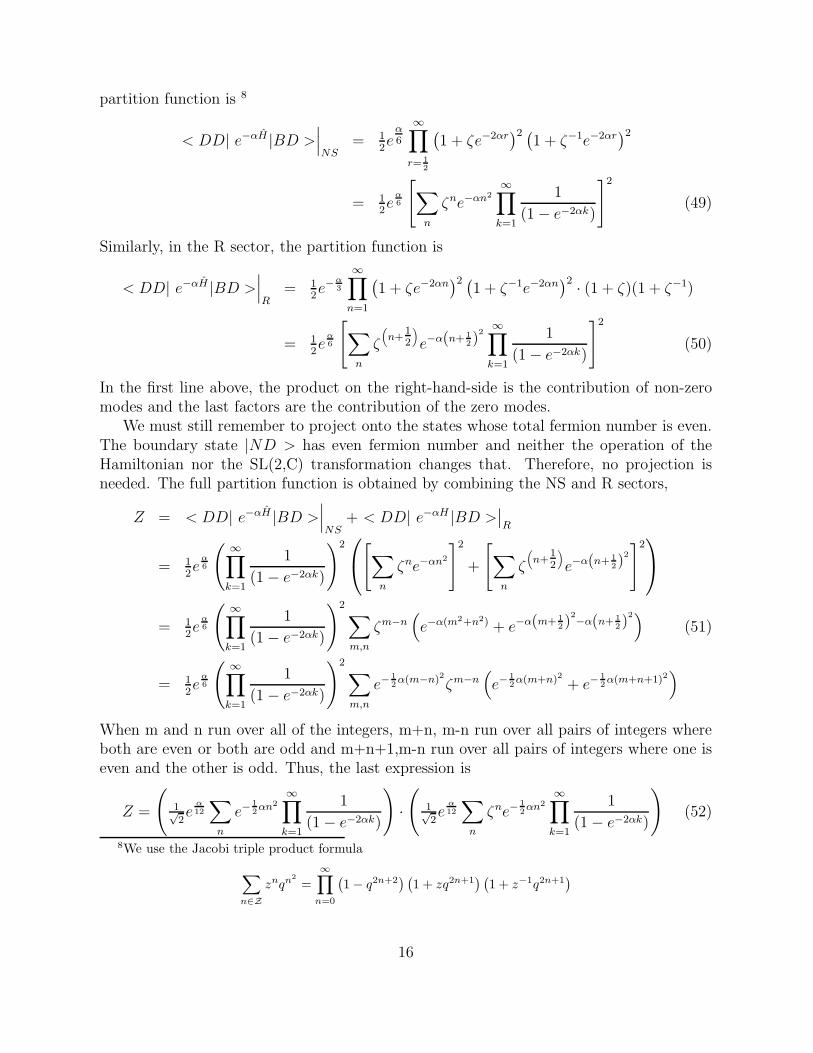
5. Band structure of the spectrum: In ref. [24] it was shown that, in some casesthe spectrum of a non-compact boson takes on an interesting band structure. Torecall what the band structure is, we begin with translation invariant theories witha free boson. If both boundary conditions are Neumann, for example, the bosonhas momentum p and energy E = p2

2. In our construction, we begin by treating it

as a compact boson, whose momenta are quantized, 1√2p = n. The presence of the

Wilson line term in the action shifts these momenta by a constant, 1√2p = n + A

and the energy is E = (n+ A)2. We see that the spectrum is split into “energybands”. The integer n labels the band and as we vary A over its range (say −1

2to

+12, we sweep through the energies in a given band. Of course, for the free boson

with Neumann boundary conditions, combining the bands just recovers the parabolicspectrum E = 1

2p2 with p varying over the real numbers.

Now, we have observed that the addition of a boundary interaction with discretetranslation symmetry changes the boson momenta and energies to 1√

2p = n+ δ(A, n)

and E(n,A) = (n+ δ(A, n))2, respectively. As we sweep A over its range of allowed

20

values, −12< A ≤ 1

2, 1√

2p = n + δ(A, n) varies over a range of momenta and E(n,A)

varies over the n’th energy band.

In eqs. (6) and (7) we see that δ(A, n) does not depend on n, reduces to δ0 = Afor a boson with Neumann boundary conditions at both boundaries, and otherwiseis a function of the coupling constants of the boundary sine-Gordon theory and Agiven in (7). The example of the system with a Neumann boundary condition plusboundary sine-Gordon with particular values of the coupling constants are shown infig. (1).

When the translation invariance is broken entirely, as in the case of a Dirichlet bound-ary condition, we can still think of the position of the D-brane as a parameter analo-gous to A. Translation invariance can be restored by integrating over this parameter.For example, in eq. (54), if the D-brane were placed at X = x0, rather than X = 0,the energy shift would be replaced by

δ =1

2πcos−1 π

2

(

geix0 + ge−ix0)

. (65)

This formula is obtained from (7) by putting (g1, g1, A1) → (g, g, A) and (g2, g2, A2) →(

− 1πeix0,− 1

πe−ix0 , 0

)

.

As x0 varies between −π and π, δ sweeps across an “energy band”.

0

0.2

0.4

0.6

0.8

1

1.2

1.4

1.6

1.8

-0.4 -0.2 0 0.2 0.4

p2

A

Band structure for g = g = 1√2π

n = 0

n = −1

n = 1

n = −2

Figure 1: The energy bands in the spectrum of a single boson on a strip with a Neumannboundary condition at one boundary and boundary sine-Gordon interaction on the other.

21

4 Rational radii

In the boson field theory quantized on the cylinder, the dependence on the compactificationradius of the boson resides entirely in the allowed momentum quantum numbers. The totalmomentum, 1√

2(pXL + pXR) must come in units of integer/R whereas the dual momentum

1√2(pXL − pXR) must be integers·R. So far, we have considered the case of self-dual radius,

R = 1. In this section, we will consider other radii, which are rational numbers R = MN

where M and N are co-prime integers.It has been shown [29, 20] that conformal boundary states at rational radii can be

found by simply choosing that subset of the states contained in the boundary state at theself-dual radius which have the correctly quantized momenta. They further argue that,together with the SL(2,C) boundary states that we have already discussed, these exhaustthe set of possible conformal boundary states of a system with one massless boson in thebulk.

Since, in the fermion description of the theory, the momenta are fermion numbers,this means that these states can be found by projecting the boundary states at the self-dual radius onto sectors with fixed fermion number. If we consider the X-boson with theidentification

X ∼ X + 2πM

Nwhere M and N are mutually prime, then the momentum and wrappings are quantized as

1√2pX =

1√2(pXL + pXR) = K

N

M,

1√2wX =

1√2(pXL − pXR) = L

M

N(66)

where K and L are integers. From these, we must choose states that are already in thespectrum at the self-dual radius, i.e. where the right-hand-sides of these equations areequal to integers. This means that we can only find states where K = QM and L = RNwith (Q,R) integers. That is,

1√2(pXL + pXR) = K

N

M= QN ,

1√2(pXL − pXR) = L

M

N= RM (67)

Now, using (25), (28a), (28b) and (29), we see that, in terms of the current algebracharges, these imply the constraints

J3L − J3

R = QN , J3L + J3

R = RM (68)

where Q and R are any integers. We can impose these as constraints on the boundary stateby operating with projection operators,

|BM/N , D >=1

MN

N−1∑

Q=0

M−1∑

R=0

e2πiQ

N(J3

L−J3R)e2πi

RM

(J3L+J

3R)|BD > (69)

Since this projection does not involve the current algebra Ja′ in (30), it does not disturbthe Dirichlet boundary condition for the Y-boson. We can also still take the Y-boson tobe compact with the self-dual radius.

22

The expression in (69) is a sum over the SL(2,C) boundary states. The state in eachterm in the sum is of the form

e2πiQ

N(J3

L−J3R)e2πi

RM

(J3L+J

3R)|BD > = e2πi(

Q

N+ R

M )J3Le−iθ·JLe2πi(−

Q

N+ R

M )J3R|ND >

= e2πi(Q

N+ R

M )J3Le−iθ·JLe2πi(−

Q

N+ R

M )J3L|ND > . (70)

This effectively replaces the matrix U by the transformed matrix

U → eπi(QN− R

M )σ3Ue−πi(QN+ R

M )σ3 =

(

e−2πi(A+R/M)√

1− π2gg −iπge2πiQ/N−iπge−2πiQ/N e−2πi(A+R/M)

√

1− π2gg

)

.(71)

Thus, each of the boundary states is the boundary state for a boundary sine-Gordon theorywith the replacement of parameters

g → ge2πiQ/N , A→ A+R/M. (72)

Then, a field theory of a boson on a strip for which |BM/ND > in (69) is the correctboundary state has the partition function

Z =1

MN

N−1∑

Q=0

M−1∑

R=0

∫

[dX ] e−S[X,M,N ;Q,R] (73)

where the Euclidean action is

S =1

4π

∫ β

0

dτ

∫ π

0

dσ(

∂τX(τ, σ)2 + ∂σX(τ, σ)2)

+ i

∫ β

0

dτ(A+R

M)∂τX(τ, 0)

+

∫ β

0

dτ(g

2eiX(τ,0)+2πiQ

N +g

2e−iX(τ,0)−2πiQ

N

)

(74)

Note that the potential term in the action is invariant under simultaneous translationsX → X + 2π·integer/N and Q → Q−integer mod N. Then, we use the prescription ofSect. 1.1 to sum over Bloch wave-number, elongating the period from X → X + 2π 1

Nto

X → X + 2πMN. The remaining parameter has the identification A ∼ A+ N

M.

The constraint on the boundary state in (69) is reminiscent of a Gauss’ law constraintin a gauge field theory, with the unusual feature that it requires invariance only underdiscrete subgroups of U(1). It is easy to imagine that such a theory could be an effectivefield theory for a discrete gauge theory. Such theories are known to arise when a continuousgauge symmetry is not fully spontaneously broken, but leaves a discrete residual gaugegroup [36].

5 Disc Amplitude

In this section, we will consider the disc correlation functions

< pXL, pXR|B >

23

These are called disc correlation functions because they should reproduce the Euclideanpath integral where the two dimensional space-time is a disc, rather than strip, with theboundary interaction living at the boundary of the disc, and the bulk vertex operator: eipXLXL+ipXRXR : inserted at the center. The result is

214 < pXL, pXR|B >=

[−iU12]√2pXL pXL = pXR > 0

[U11]√2pXL pXL = −pXR > 0

[U22]−√2pXL −pXL = pXR > 0

[−iU21]−√2pXL pXL = pXR < 0

0 |pXL| 6= |pXR|

(75)

This formula applies to both cases where either both of 1√2pXL and 1√

2pXR are integers or

both are half-odd-integers.We can use eq. (75) to compute the overlap of the boundary state with the state which

is a vacuum for all bulk boson oscillators and which is an eigenstate of the average positionof the X−boson. We define the variables

X0 =1√2(xL + xR) , X0 =

1√2(xL − xR)

and the position eigenstates of these operators as

|X0, X0 >=1

2π

∑

π

e−i 1√

2(pXL+pXR)X0−i

1√2(pXL−pXR)X0 |pXL, pXR > . (76)

Then, taking the matrix element and doing the geometric sums over momenta obtains

214 < X0, X0|B >= 1

2π

[

1

1− U11eiX0

+1

1− U22e−iX0

+1

1 + iU12eiX0+

1

1 + iU21e−iX0− 3

]

(77)

This formula can be applied to the case of a non-compact boson, and a compact bosonwith self-dual and fractional radii. The appropriate expressions are presented in eqs. (10)-(12).

In order to illustrate the simplicity of the computation, we spell it out in some detailbelow. We arrive at this result be computing the state< pXL, pXR, pY L = 0, pY R = 0|BD >.The overlap with the zero momentum states for the Y -boson with its Dirichlet state givesa factor of 2−1/4. Thus, the Y -boson contribution is trivial and we can later cancel it bymultiplying by 21/4.

Recall that pY L = 1√2(π1L − π2L) and pY R = 1√

2(π1R − π2R). For this reason, we need

to consider states whose momenta obey π1L = π2L ≡ πL = 1√2pXL and π1R = π2R ≡ πR =

1√2pXR.

Also, recall that, in the NS sector, (πL, πR) are both integers, whereas in the R sector(πL, πR) are both half-odd-integers. Both of these possibilities must be considered. Sincethe boundary states have even fermion number, no further GSO projection is needed.

24

The total boson momentum is related to total fermion number,

π1L =

∫

dσ2π

: ψ†1Lψ1L : , π1R = −

∫

dσ2π

: ψ†1Rψ1R : (78a)

π2L = −∫

dσ2π

: ψ†2Lψ2L : , π1R =

∫

dσ2π

: ψ†2Rψ2R : (78b)

In the NS sector, the fermion vacuum is unique and the fermion number is quantizedas integers. The above equations show that the boson momentum is equal to ± the totalfermion number of the states there.

In the R-sector, the vacuum is degenerate and the vacuum states | − − − − > havefermion numbers (−1/2,−1/2,−1/2,−1/2) and π1L = −1/2, π1R = 1/2, π2L = 1/2 andπ2R = −1/2. Operating fermion operators change these by integers, so that the wholespectrum of fermion numbers and momenta are half-odd-integers.

Then, following ref. [19], we observe that the boson momentum eigenstates which haveno boson oscillators excited correspond to fermion states where all fermion states are filledup to a Fermi level. The fermion number of each type of fermions is equal (up to signs) tothe momentum of the corresponding boson state.

5.1 NS Sector

In the NS-sector, the πL and πR are integers. We denote the states with these values of bosonmomentum (and vanishing Y -momenta) and no boson oscillators excited by |πL, πR >.

We shall require the fermion representation of the boson momentum state in bra-form.The following are the states of the NS sector,

πL > 0 , πR > 0 < πL, πR| = < 0|πL−

12

∏

r=12

(

ψ†2rψ1r

)

πR−12

∏

r=12

(

ψ2rψ†1r

)

(79a)

πL > 0 , πR < 0 < πL, πR| = < 0|πL−

12

∏

r=12

(

ψ†2rψ1r

)

−πR−12

∏

r=12

(

ψ1rψ†2r

)

(79b)

πL < 0 , πR > 0 < πL, πR| = < 0|−πL−

12

∏

r=12

(

ψ†1rψ2r

)

πR−12

∏

r=12

(

ψ2rψ†1r

)

(79c)

πL < 0 , πR < 0 < πL, πR| = < 0|−πL−

12

∏

r=12

(

ψ†1rψ2r

)

−πR−12

∏

r=12

(

ψ1rψ†2r

)

. (79d)

The phases of these states are fixed by their overlaps with |DD > and |ND > which,recalling the known forms of these states in boson variables, must all be either zero or one.

25

The boundary state in the NS sector is given in eq. (42) which we copy here for conve-nience of the reader:

|B,D >NS=1√2

∞∏

r=12

exp[

ψ†−rU

−1iσ1ψ−r − ψ†−riσ

1Uψ−r

]

|0 > . (80)

Then, we can take the matrix elements of the momentum states and the boundary stateto obtain:

πL > 0, πR > 0

< πL, πR|B,D >NS = 1√2< 0|

πL−12

∏

r=12

(

ψ†2r + ψ†

a,−r[iσ1U ]a2

)(

ψ1r + [U−1iσ1]1aψa,−r

)

·

πR−12

∏

r=12

(

ψ2r − [iσ1U ]2aψa,−r

)(

ψ†1r − ψ†

a,−r[U−1iσ1]a1

)

|0 >

= 1√2(−iU12)

2πL δ(πL − πR) (81)

πL > 0, πR < 0

< πL, πR|B,D >NS = 1√2< 0|

πL−12

∏

r=12

(

ψ†2r + ψ†

a,−r[iσ1U ]a2

)(

ψ1r + [U−1iσ1]1aψa,−r

)

·

−πR−12

∏

r=12

(

ψ1r − [iσ1U ]1aψa,−r

)(

ψ†2r − ψ†

a,−r[U−1iσ1]a2

)

|0 >

= 1√2(U11)

2πL δ(πL + πR) (82)

πL < 0, πR > 0

< πL, πR|B,D >NS = 1√2< 0|

−πL−12

∏

r=12

(

ψ†1r + ψ†

a,−r[iσ1U ]a1

)(

ψ2r + [U−1iσ1]2aψa,−r

)

·

πR−12

∏

r=12

(

ψ2r − [iσ1U ]2aψa,−r

)(

ψ†1r − ψ†

a,−r[U−1iσ1]a1

)

|0 >

= 1√2(U22)

−2πL δ(πL + πR) (83)

26

πL < 0, πR < 0

< πL, πR|B,D >NS = 1√2< 0|

−πL−12

∏

r=12

(

ψ†1r + ψ†

a,−r[iσ1U ]a1

)(

ψ2r + [U−1iσ1]2aψa,−r

)

·

−πR−12

∏

r=12

(

ψ1r − [iσ1U ]1aψa,−r

)(

ψ†2r − ψ†

a,−r[U−1iσ1]a2

)

|0 >

= 1√2(−iU21)

−2πL δ(πL − πR) (84)

This summarizes the overlap of momentum eigenstates with the boundary state in theNS sector.

5.2 R-sector

In the R-sector, the momenta are half-odd-integral and the momentum states of the X-boson are

πL > 0, πR > 0, < πL, πR| = < +−−+ |πL−

12

∏

n=1

(

ψ†2nψ1n

)

πR−12

∏

n=1

(

ψ2nψ†1n

)

(85a)

πL > 0, πR < 0, < πL, πR| = i < ++−− |πL−

12

∏

n=1

(

ψ†2nψ1n

)

−πR−12

∏

n=1

(

ψ1nψ†2n

)

(85b)

πL < 0, πR > 0, < πL, πR| = −i < −−++ |−πL−

12

∏

n=1

(

ψ†1nψ2n

)

πR−12

∏

n=1

(

ψ2nψ†1n

)

(85c)

πL < 0, πR < 0, < πL, πR| = < −++− |−πL−

12

∏

n=1

(

ψ†1nψ2n

)

−πR−12

∏

n=1

(

ψ1nψ†2n

)

. (85d)

Here, again, the phases have been adjusted so that the matrix elements of these stateswith the |DD > and |ND > are always either one or zero, just as the phases of the bosonstates (21a)-(21b) (with A = 0) with boson momentum states would be.

The R-sector boundary state is given in eq. (43) which we copy here for the reader’sconvenience:

|BD >R= 2−12

∞∏

n=1

exp[

ψ†−nU

−1iσ1ψ−n − ψ†−niσ

1Uψ−n

]

exp[

ψ†0U

−1iσ1ψ0

]

| −+−+ > .

(86)

27

Then, the matrix elements are taken as

πL > 0, πR > 0

< πL, πR|B,D >R =1√2< +−−+ |

πL−12

∏

n=1

(

ψ†2,n + ψ†

a,−n[iσ1U ]a2

)(

ψ1,n + [U−1iσ1]1aψa,−n

)

·

πR−12

∏

n=1

(

ψ2,n − [iσ1U ]2aψa,−n

)(

ψ†1,n − ψ†

a,−n[U−1iσ1]a1

)

exp[

ψ†0U

−1iσ1ψ0

]

| −+−+ >

=1√2(−iU12)

2πL δ(πL − πR), (87)

πL > 0, πR < 0

< πL, πR|B,D >R =i√2< ++−− |

πL−12

∏

n=1

(

ψ†2,n + ψ†

a,−n[iσ1U ]a2

)(

ψ1,n + [U−1iσ1]1aψa,−n

)

·

−πR−12

∏

n=1

(

ψ1,n − [iσ1U ]1aψa,−n

)(

ψ†2,n − ψ†

a,−n[U−1iσ1]a2

)

exp[

ψ†0U

−1iσ1ψ0

]

| −+−+ >

=1√2(U22)

2πL δ(πL + πR), (88)

πL < 0, πR > 0

< πL, πR|B,D >R = − i√2< −−++ |

−πL−12

∏

n=1

(

ψ†1,n + ψ†

a,−n[iσ1U ]a1

)(

ψ2r + [U−1iσ1]2aψa,−n

)

·

πR−12

∏

n=1

(

ψ2,n − [iσ1U ]2aψa,−n

)(

ψ†1,n − ψ†

a,−n[U−1iσ1]a1

)

exp[

ψ†0U

−1iσ1ψ0

]

| −+−+ >

=1√2(U11)

−2πL δ(πL + πR), (89)

28

πL < 0, πR < 0

< πL, πR|B,D >R =1√2< −++− |

−πL−12

∏

n=1

(

ψ†1,n + ψ†

a,−n[iσ1U ]a1

)(

ψ2r + [U−1iσ1]2aψa,−n

)

·

−πR−12

∏

n=1

(

ψ1,n − [iσ1U ]1aψa,−n

)(

ψ†2,n − ψ†

a,−n[U−1iσ1]a2

)

exp[

ψ†0U

−1iσ1ψ0

]

| −+−+ >

=1√2(−iU21)

−2πL δ(πL − πR). (90)

We see that the overlap of momentum states with R states has a very similar form tothe overlaps with NS states.

6 Conclusions

The critical theory which we have discussed in this Paper should be difficult to producein a realistic system. The reason for this is that, when the parameters are tuned so thatprecisely the exactly marginal boundary operator is allowed by the periodicity of the boson,a bulk operator with the same periodicity is allowed in the bulk. Moreover, : eiX : is arelevant perturbation in the bulk, it drives a Kosterlitz Thouless transition which gaps thespectrum there, nullifying our possibility of finding the critical theory on the boundary.

In string theory, this is the Hagedorn behavior. When a coordinate of the bosonic stringis compactified and the radius is lowered from infinity, we expect to see a phase transitionwhen R =

√2, before we arrive at the self-dual value R = 1. In the string theory, this is

fixed by going to the superstring where super-partners of the boson provide stability. Itwould be interesting to understand this better in the context of our present analysis.

Further, although the self-dual radius R = 1 lies in the unstable regime, a large numberof the fractional radii R =M/N do not. On general grounds, we expect that their criticalstates are less stable than the self-dual state – they contain fewer states, so should havesmaller entropy and therefore larger free energy – they would avoid the Kosterlitz-Thoulesstransition in the bulk.

The boundary sine-Gordon theories which have fractional periods are apparently non-local. We have presented them as theories at the dual radius with the addition of a discretegauge invariance. Such theories are indeed known to arise in models of Josephson-junctionarrays [37]-[39] and whether the conformal field theories with rational radii can be realizedthere is an interesting question.

The fermionic boundary states are simple and easy to work with. It should be straight-forward to use them to check some important previous computations which used othertechniques. One example is the closed string emission amplitudes for the rolling tachyonwhich were computed in [40], and should easily be accessible in the fermion picture.

29

Acknowledgement: The authors thank Volker Schomerus and Ian Affleck for extensiveand informative discussions. This work is supported in part by NSERC of Canada, bythe Pacific Institute for Theoretical Physics and by KOSEF of Korea through CQUeST(Center for Quantum Space Time). The work of TL is also supported by Kangwon NationalUniversity through the Research Fund for 2003 Faculty Research Abroad.

References

[1] A. Schmid, Phys.Rev.Lett. 51, 1506 (1983).

[2] F. Guinea, V. Hakim and A. Muramatsu, “Diffusion and localization of a particle ina periodic potential coupled to a dissipative environment,” Phys. Rev. Lett. 54, 263(1985).

[3] M.P.A. Fisher and W. Zwerger, “Quantum Brownian motion in a periodic potential,”Phys.Rev. B32, 4190 (1985).

[4] C. G. Callan and L. Thorlacius, “Open String Theory As Dissipative Quantum Me-chanics,” Nucl. Phys. B 329, 117 (1990).

[5] L.I. Glazman and A.I. Larkin, “New quantum phases in a one-dimensional junctionarray,” Phys.Rev.Lett. 79, 3736 (1997) [arXiv:cond-mat/9809118].

[6] R. Fazio and H. van der Zant, ”Quantum Phase transitions and Vortex dynamics inSuperconducting networks”, Phys. Rep. 355, 235 (2001)

[7] D. Giuliano and P. Sodano, “Effective boundary field theory for a Josephson junctionchain with a weak link”, Nucl. Phys. B711, 480-504, (2005) [arXiv:cond-mat/0501378].

[8] C. G. Callan and D. Freed, “Phase diagram of the dissipative Hofstadter model,” Nucl.Phys. B 374, 543 (1992) [arXiv:hep-th/9110046].

[9] C. G. Callan, A. G. Felce and D. E. Freed, “Critical theories of the dissipative Hofstadtermodel,” Nucl. Phys. B 392, 551 (1993) [arXiv:hep-th/9202085].

[10] I. Affleck and A. W. W. Ludwig, “Critical Theory Of Overscreened Kondo FixedPoints,” Nucl. Phys. B 360, 641 (1991).

[11] I. Affleck and A. W. W. Ludwig, “The Kondo Effect, Conformal Field Theory AndFusion Rules,” Nucl. Phys. B 352, 849 (1991).

[12] C. L. Kane and M. P. A. Fisher, “Transmission through barriers and resonant tunnelingin an interacting one-dimensional electron gas,” Phys.Rev. B46, 15233 (1992).

[13] C.L. Kane and M.P.A. Fisher, “Contacts and Edge State Equilibration in the Frac-tional Quantum Hall Effect” cond-mat/9506116

30

[14] M. Oshikawa, C. Chamon and I. Affleck, “Junctions of three quantum wires,” Phys.Rev. Lett. 91, 206403 (2003) [arXiv:cond-mat/0509675].

[15] E. Witten, “On background independent open string field theory,” Phys. Rev. D 46,5467 (1992) [arXiv:hep-th/9208027].

[16] S. L. Shatashvili, “Comment on the background independent open string theory,”Phys. Lett. B 311, 83 (1993) [arXiv:hep-th/9303143].

[17] S. L. Shatashvili, “On the problems with background independence in string theory,”Alg. Anal. 6, 215 (1994) [arXiv:hep-th/9311177].

[18] A. Sen, “Rolling tachyon,” JHEP 0204, 048 (2002) [arXiv:hep-th/0203211].

[19] T. Lee and G. W. Semenoff, “Fermion representation of the rolling tachyon boundaryconformal field theory,” JHEP 0505, 072 (2005) [arXiv:hep-th/0502236].

[20] M. R. Gaberdiel and A. Recknagel, “Conformal boundary states for free bosons andfermions,” JHEP 0111, 016 (2001) [arXiv:hep-th/0108238].

[21] A. Recknagel and V. Schomerus, “Boundary deformation theory and moduli spaces ofD-branes,” Nucl. Phys. B 545, 233 (1999) [arXiv:hep-th/9811237].

[22] C. Ahn and R. I. Nepomechie, “Finite size effects in the XXZ and sine-Gordon modelswith two boundaries,” Nucl. Phys. B 676 (2004) 637 [arXiv:hep-th/0309261].

[23] C. Ahn, Z. Bajnok, R. I. Nepomechie, L. Palla and G. Takacs, “NLIE for hole excitedstates in the sine-Gordon model with two boundaries,” Nucl. Phys. B 714, 307 (2005)[arXiv:hep-th/0501047].

[24] J. Polchinski and L. Thorlacius, “Free fermion representation of a boundary conformalfield theory,” Phys. Rev. D 50, 622 (1994) [arXiv:hep-th/9404008].

[25] C. G. . Callan, I. R. Klebanov, A. W. W. Ludwig and J. M. Maldacena, “Ex-act solution of a boundary conformal field theory,” Nucl. Phys. B 422, 417 (1994)[arXiv:hep-th/9402113].

[26] K. R. Kristjansson and L. Thorlacius, “Correlation functions in a c = 1 boundaryconformal field theory,” JHEP 0501, 047 (2005) [arXiv:hep-th/0412175].

[27] I. R. Klebanov and A. M. Polyakov, “Interaction of discrete states in two-dimensionalstring theory,” Mod. Phys. Lett. A 6, 3273 (1991) [arXiv:hep-th/9109032].

[28] N. Seiberg and E. Witten, “Spin Structures In String Theory,” Nucl. Phys. B 276,272 (1986).

[29] M. R. Gaberdiel, A. Recknagel and G. M. T. Watts, “The conformal boundary statesfor SU(2) at level 1,” Nucl. Phys. B 626, 344 (2002) [arXiv:hep-th/0108102].

31

[30] V. Schomerus, “Non-compact string backgrounds and non-rational CFT,”arXiv:hep-th/0509155.

[31] M. R. Gaberdiel, “2D conformal field theory and vertex operator algebras,”arXiv:hep-th/0509027.

[32] F. Larsen, A. Naqvi and S. Terashima, “Rolling tachyons and decaying branes,” JHEP0302, 039 (2003) [arXiv:hep-th/0212248].

[33] N. R. Constable and F. Larsen, “The rolling tachyon as a matrix model,” JHEP 0306,017 (2003) [arXiv:hep-th/0305177].

[34] M. R. Gaberdiel and M. Gutperle, “Remarks on the rolling tachyon BCFT,” JHEP0502, 051 (2005) [arXiv:hep-th/0410098].

[35] H. Kogetsu and S. Teraguchi, “Massless boundary sine-Gordon model coupled to ex-ternal fields,” JHEP 0501, 048 (2005) [arXiv:hep-th/0410197].

[36] L. M. Krauss and F. Wilczek, “Discrete gauge symmetry in continuum theories,” Phys.Rev. Lett. 62, 1221 (1989).

[37] B. Doucot, M.V. Feigel’man, L.B. Ioffe, “Topological order in the insulating Josephsonjunction array”, Phys. Rev. Lett. 90, 107003 (2003), cond-mat/0211146

[38] L.B. Ioffe, M.V. Feigel’man, “Possible realization of an ideal quantum computer inJosephson junction array”, Phys. Rev B66, 224503 (2002), cond-mat/0205186.

[39] B. Doucot, L. B. Ioffe and J. Vidal, “Discrete non-Abelian gauge theories in two-dimensional lattices and their realizations in Josephson-junction arrays,”, Phys. Rev.B69, 214501 (2004), arXiv:cond-mat/0302104.

[40] N. Lambert, H. Liu and J. Maldacena, “Closed strings from decaying D-branes,”arXiv:hep-th/0303139.

32