1

Credit Scoring Models: A Comparison between Crop and Livestock Farms

Seda Durguner, Peter J. Barry and Ani L. Katchova

May 2006

Contact Author: Seda Durguner University of Illinois 326 Mumford Hall, MC-710 1301 West Gregory Drive Urbana, IL 61801 Tel: (217) 244-2466 E-mail: sdurgun2@uiuc.edu

Selected paper prepared for presentation at the American Agricultural Economics Association Meeting, Long Beach, California, July 23-26, 2006

Copyright 2006 by Durguner, Barry, and Katchova. All rights reserved. Readers may make verbatim copies of this document for non-commercial purposes by any means, provided that this copyright notice appears on all such copies.

Seda Durguner is a graduate student, Peter J. Barry is professor emeritus, and Ani L. Katchova is an assistant professor in the Department of Agricultural and Consumer Economics at the University of Illinois at Urbana-Champaign.

2

Credit Scoring Models: A Comparison between Crop and Livestock Farms

Abstract

This paper uses FBFM (Illinois Farm Business Farm Management Association) data to

analyze several key factors in the decision to categorize borrowers into acceptable or problematic

and to classify borrowers across five classes. Net worth does not play significant role in the

decision process for livestock farms, whereas it is significantly important for crop farms. For

livestock farms, tenure ratio is not significant across classes and is generally not significant across

categories depending on the cut off point used to describe acceptable or problematic borrower.

However, it is significant for crop farms. Working capital to gross farm return, return on farm

assets, and asset turnover ratio are all significant for both farm types. The operating expense to

gross farm return is not an independent variable for livestock farms whereas an independent and

significant variable for crop farms.

Key words: acceptable borrower, classes, credit scoring, crop farms, cut off point, livestock farms,

and problematic borrower.

3

Credit Scoring Models: A Comparison between Crop and Livestock Farms

I) Introduction

Proposed in 1988, the Basel I Capital Accord, set guidelines for minimum capital

requirements for financial institutions based on their exposed credit risk. Even though it was

intended for G10 countries, it was adopted by 120 countries. One disadvantage of Basel I was that

it did not differentiate financial institutions’ credit risk by counterparty or loan. Banks with

different risk exposures and risk ratings could have the same capital requirements. Basel II is an

improvement over Basel I. It uses credit ratings from external rating agencies to define the

categories and weights, and these categories and weights are individualized for the assessment of

credit risks of each financial institution (Mendoza & Stephanou, 2005). Consequently, under Basel

II, there is not a single risk measurement and capital management approach. They are adjusted for

the characteristics of diverse financial institutions (Featherstone, Roessler, and Barry, 2006).

Hence, under Basel II we see more refined models for determining capital requirements and these

models change based on the different credit risk exposure and risk ratings of each financial

institution.

Basel II’s recognition of different loan types is consistent with the Farm Credit System’s

treatment of agricultural loan types. For instance, the Farm Credit System which is the major

lender for agricultural loan, has 5 aggregate loan types - commercial farm loan, farm real estate

loan, agribusiness loan, rural housing loan, and small loans. Each of these loan types uses its own

credit scoring model. Thus, this implies that in its credit evaluations, the Farm Credit System

recognizes the diversity in agriculture. However, this raises the question whether differences in

types of farms within the commercial farm category should be considered. Among farm types,

there are considerable differences in rates of return on assets, leverage ratios and liquidity. For

4

instance, Boessen, Featherstone, Langemeier, and Burton (1990) identify large differences

between the return on assets and leverage ratios for swine farms, and beef cow herd farms, with

swine farms having three times more return on assets rates than beef cow herd farms and a

leverage ratio of 0.25 compared to 0.16 for beef cow herd farms. Due to differences between farm

types, the Farm Credit System might need to extend their risk rating system by applying different

models for different farm types. These multiple credit scoring models can prevent costs of

misclassifying borrowers that might be caused by not differentiating between farm types.

The misclassification problem exists also for regional credit scoring models. Lenders

located in different regions typically have different credit scoring models. For instance, lenders in

Illinois use a different credit scoring model than a lender in another region. However, each lender

uses a single credit scoring model for all farm types and this credit scoring model is more

representative of the farm type dominant in that region. For instance, Miller and LaDue (1989)

developed a credit scoring model for a bank in New York and focused on dairy farms, while

Luftburrow, Barry and Dixon (1984) for pricing purposes developed only one credit scoring model

for five production credit associations in Illinois, with three of these associations focusing on grain

farms and two other associations having more diverse borrower types including hog, dairy and

beef farms. Even though separate models have been developed for separate regions, these models

do not take into consideration the variability in farm types that exist in the same region. Separate

models are needed for the same region across farm types to prevent misclassification of borrowers.

In the US, the development of different credit scoring models for a region has not been

examined, but such research has been done for Canada. Turvey and Brown (1990) found that for

Canada’s Farm Credit Corporation, farm type played an important role in the development of

credit scoring models.

5

The Illinois Farm Business Farm Management Association has analyzed farms’ financial

measures by farm types: hog, grain, dairy and beef. This analysis shows that financial

characteristics differ across hog, dairy, beef and grain farms in Illinois. Due to the differences in

financial characteristics across farm types, it is expected that the system reflects differences in

farm types in Illinois.

Based on the call by previous research for analyzing different farm types (Splett et

al.,1994; Phillips and Katchova, 2004; Lufburrow, Barry, and Dixon, 1984) and the expectation

that the system reflects differences in farm types in Illinois, the objective of this study is to: 1) to

examine the important factors that determine the overall creditworthiness of a borrower by logit

model, 2) to analyze whether credit scoring models differ across livestock farms (including hog,

dairy, beef) and crop farms (grain farms) in Illinois.

The results will be informative to lenders as they consider further extensions and

refinements of their risk rating systems in response to the new Basel Accord. Using models

specific to farm types will reduce the costs of misclassification, and provide more equitable

treatment of alternative farm types, risk-adjusted pricing across farm types, and greater efficiency

in credit valuation. Further, the costs for implementing and extension of multiple credit scoring

models to include farm types will be relatively low and subsequent operating costs will be minimal

given that data are available and the estimation procedure is in place.

II) Literature review

Nayak and Turvey (1997) argue that the misclassification arises due to asymmetric

information and adverse selection. Lenders use screening devices to prevent adverse selection. One

screening device lenders use is to offer high interest rates to all borrowers. The problem with this

6

approach is that borrowers may not fully understand the underlying risks associated with these

high interest rates. An alternative screening device is to use a credit scoring model which provides

an objective measure of borrower risk. Even though credit scoring models do not eliminate the

asymmetric information and adverse selection, they minimize it. Many lenders in US and Canada

have adopted formal credit evaluation models to minimize adverse selection and asymmetric

information.

Nayak and Turvey (1997) also state that misclassification errors can be categorized under

two types, type 1 and type 2 errors. Type 1 error occurs when a bad borrower is accepted as a good

borrower resulting in adverse selection of high-risk borrowers. The cost of this error are the loans

foreclosed or in default temporarily. Specifically, costs include lost principal, lost interest on

principal during the period of litigation and foreclosure, costs in administration, legal fees,

insurance coverage and property taxes. Type 2 error occurs when a low-risk borrower is adversely

rejected, and the loan is given to alternative borrower. Type 2 error has 3 components. The first is

the foregone interest income from adverse rejection of a good loan or low-risk borrower. The

second is the interest income obtained in case the alternative borrower is a good borrower, and the

third is the lost money in case the alternative borrower is a bad borrower. Losses include the

difference in expected profit foregone from the low-risk borrower and the expected profit from the

alternative borrower.

Since type 2 error is not observable, it can be argued that rejecting a good loan or low-risk

borrower is not very costly. However, under the assumption that the lender will lend the money to

an alternative borrower, the cost associated with type 2 error can be high if the alternative

borrower has high credit risk. In this situation, the lost revenue from an adversely rejected good

loan may not be recoverable and the possible type 1 error due to the alternative borrower being

7

high credit risk but being adversely accepted increases the cost of Type 2 error. In general, the

misclassification errors are costly to the lender and they influence the overall profitability of the

loan portfolio. Estimating separate credit scoring models for different farm types in the same

region will minimize these classification errors.

As mentioned, in general the credit scoring models of lenders do not reflect benchmarks

such as farm type. Instead lenders adjust their models to farm types subjectively. However,

previous research shows that bankers intend to use less subjective and more quantitative methods.

For instance, Featherstone, Roessler, and Barry (2006) state that lenders use statistical rating

systems and professional judgment and experience in their rating processes, because lenders

believe that professional judgment and experience provide greater accuracy, confidence and

flexibility in their rating systems. However, they also state that, with Basel II, lenders started using

more advanced rating systems. As lenders improve on their risk-rating systems, they focus more

on quantitative assessment rather than subjective methods since quantitative assessment shortens

the decision process and gives more standardized results. Hence, quantitative methods such as

credit scoring models, which are recently the focus of lenders, are an important tool for bankers.

Turvey and Brown (1990) looked at whether differences in farm types and regions should

be accounted for in credit scoring models, but they did not look at what explanatory factors

became important across different farm types and regions. The advantage of their study is that they

use national data base, resulting in a diverse set of farms. They found that for Canada’s Farm

Credit Corporation, farm type played an important role in the development of credit scoring

models. However, this has not been analyzed for the US. In US, the lenders service specific

regions and are not nationalized. Consequently, most of the credit scoring models are regional.

While credit scoring models differ from region to region, lenders tend to use a single credit scoring

8

model for all farm types in that region. For instance Miller and LaDue (1989) developed a credit

scoring model for a bank in New York and focused on dairy farms while Luftburrow, Barry and

Dixon (1984) developed one credit scoring model for five production credit associations in Illinois,

with three of production credit associations focusing on grain farms and the other two association

having diverse borrower type such as dairy, beef and hog farms.

Here we investigate the importance of developing different credit scoring models for a

specific region in US. This study differs from Turvey and Brown (1990) by determining whether

different explanatory factors become important for credit scoring models across livestock farms

and crop farms.

Previous research also states that the effect of different farm types on credit scoring

models, credit risk migration analysis should be analyzed, as well as on the effect of credit scoring

in pricing decisions. For instance, Splett et al. (1994) stated that lenders should develop credit

scoring models based on different structural characteristics such as loan structure, and farm type.

Phillips and Katchova (2004) stated that the migration analysis differences could also occur across

farm types. Lufburrow, Barry and Dixon (1984) stated that testing the usefulness of credit scoring

models in pricing decisions for different farm types might be a good future research.

III) Data

This paper uses FBFM (Illinois Farm Business Farm Management Association) data for

1995 to 2004, after screening for balance sheet, family living sources and uses, and economic

management analysis certifications. The farmdoc website lists debt-to-asset ratio for different

farm types, hog, dairy, beef, and grain farms. For example, for 2004 the median debt to asset ratio

for each farm type is 35.9%, 31.6%, 25.3%, and 28.5% sequentially. Based on this, it can be

9

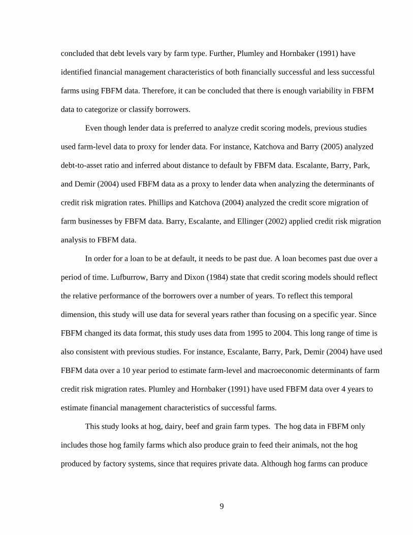
concluded that debt levels vary by farm type. Further, Plumley and Hornbaker (1991) have

identified financial management characteristics of both financially successful and less successful

farms using FBFM data. Therefore, it can be concluded that there is enough variability in FBFM

data to categorize or classify borrowers.

Even though lender data is preferred to analyze credit scoring models, previous studies

used farm-level data to proxy for lender data. For instance, Katchova and Barry (2005) analyzed

debt-to-asset ratio and inferred about distance to default by FBFM data. Escalante, Barry, Park,

and Demir (2004) used FBFM data as a proxy to lender data when analyzing the determinants of

credit risk migration rates. Phillips and Katchova (2004) analyzed the credit score migration of

farm businesses by FBFM data. Barry, Escalante, and Ellinger (2002) applied credit risk migration

analysis to FBFM data.

In order for a loan to be at default, it needs to be past due. A loan becomes past due over a

period of time. Lufburrow, Barry and Dixon (1984) state that credit scoring models should reflect

the relative performance of the borrowers over a number of years. To reflect this temporal

dimension, this study will use data for several years rather than focusing on a specific year. Since

FBFM changed its data format, this study uses data from 1995 to 2004. This long range of time is

also consistent with previous studies. For instance, Escalante, Barry, Park, Demir (2004) have used

FBFM data over a 10 year period to estimate farm-level and macroeconomic determinants of farm

credit risk migration rates. Plumley and Hornbaker (1991) have used FBFM data over 4 years to

estimate financial management characteristics of successful farms.

This study looks at hog, dairy, beef and grain farm types. The hog data in FBFM only

includes those hog family farms which also produce grain to feed their animals, not the hog

produced by factory systems, since that requires private data. Although hog farms can produce

10

grain to feed their animals, there is still considerable difference between hog and grain farms. That

is, they have different levels of leverage, equity, farm land etc. Due to that, this study considers

hog farms and grain farms as different farm types even though hog farms can as well produce

grain to feed their animals.

The ratios of return on farm assets and debt to farm operating income1 which are above or

below the mean plus or minus 3 standard deviations are deleted to resolve potential outlier

problems.

IV) Methodology and Model Specification

Theory

This section outlines the theory used. Lenders are interested in maximizing return on a loan

or minimizing the expected loss. Katchova and Barry (2005) define expected loss as:

EL= (PD) (LGD) (EAD)

Where EL is the dollar value for expected loss per farm, PD is probability of default (in

percentage), LGD is loss given default (in percentage), and EAD is the exposure at default (in

dollars). Probability of default (PD) is the frequency of loss and is determined by characteristics of

borrowers. Loss given default (LGD) is the severity of loss and is determined by characteristics of

transactions. Exposure at default (EAD) is the value of farm debt at the time of default.

Credit risk tries to identify probability of default (PD). Hence, for credit risk purposes,

lenders evaluate borrower characteristics which are defined by financial ratios. Therefore, the

credit scoring model in this study will look at financial ratios just like other previous studies

1 Farm operating income: net income from operations. For detailed calculation, please see page 55-56 in Barry, P.J., P.N. Ellinger, C.B. Baker, and J.A.Hopkin. 2000. Financial Management in Agriculture. Danville, Illinois: Interstate Publishers, Inc.

11

(Turvey and Brown, 1990; Turvey, 1991; Barry, Escalante, and Ellinger, 2002; Splett, Barry,

Dixon, and Ellinger, 1994).

Variables

Dependent variable:

The differentiation of the dependent variable across classes (lowest to highest risk class)

and categories (acceptable or problematic borrowers) will be made via loan repayment. Miller and

LaDue (1989) have emphasized that loan repayment is an objective measure. Therefore,

dependent variable (either as classes or categories) will be measured by the ability of borrowers to

repay the loan. In FBFM data, repayment capacity is defined either by capital replacement and

term debt repayment margin, or debt to farm operating income. Since this article deals with

different farm types and different farm types might have different sizes, ratios are more

appropriate than dollar measures. The ratio of debt to farm operating income, thus serves as the

dependent variable.

The dependent variable in this article is discrete rather than continuous. A discrete

dependent variable is used rather than continuous dependent variable for the following reason.

Lender is interested in which borrowers are likely to default and not default rather than ratios level.

Based on debt to farm operating income, borrowers are divided into two categories: acceptable

borrowers versus problematic borrowers. Further based on debt to farm operating income,

borrowers are assigned across classes; from 1 to 5. Class 1 represents the lowest risk, meaning

lowest debt to farm operating income while class 5 represents the highest debt to farm operating

income.

12

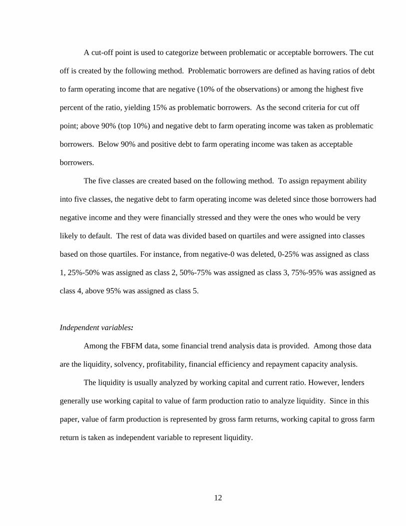
A cut-off point is used to categorize between problematic or acceptable borrowers. The cut

off is created by the following method. Problematic borrowers are defined as having ratios of debt

to farm operating income that are negative (10% of the observations) or among the highest five

percent of the ratio, yielding 15% as problematic borrowers. As the second criteria for cut off

point; above 90% (top 10%) and negative debt to farm operating income was taken as problematic

borrowers. Below 90% and positive debt to farm operating income was taken as acceptable

borrowers.

The five classes are created based on the following method. To assign repayment ability

into five classes, the negative debt to farm operating income was deleted since those borrowers had

negative income and they were financially stressed and they were the ones who would be very

likely to default. The rest of data was divided based on quartiles and were assigned into classes

based on those quartiles. For instance, from negative-0 was deleted, 0-25% was assigned as class

1, 25%-50% was assigned as class 2, 50%-75% was assigned as class 3, 75%-95% was assigned as

class 4, above 95% was assigned as class 5.

Independent variables:

Among the FBFM data, some financial trend analysis data is provided. Among those data

are the liquidity, solvency, profitability, financial efficiency and repayment capacity analysis.

The liquidity is usually analyzed by working capital and current ratio. However, lenders

generally use working capital to value of farm production ratio to analyze liquidity. Since in this

paper, value of farm production is represented by gross farm returns, working capital to gross farm

return is taken as independent variable to represent liquidity.

13

The solvency is analyzed by net worth (market), net worth (modified cost), debt/equity

(market), debt/total assets (market). Since each of them are nearly the same and the dependent

variable (debt to farm operating income) has debt concept, to prevent multi-colinearity issue, net

worth (market) is taken as independent variable rather than debt/equity or debt/total assets.

The profitability is analyzed by net farm income and net non-farm income. These are

different measurements for FBFM data because FBFM data involves large farms. Since, small

farms rely more on net non-farm income whereas large farms use net farm income, using these two

ratios together will not give multi-colinearity problem. Further profitability is analyzed by net

income less withdrawals. To calculate this ratio, net farm income and net non-farm income are

used together. If net income less withdrawals is used, net farm income and net non-farm income

cannot be used. Other than these, profitability is analyzed by return on farm assets (market) and

return on farm equity (market). This article will use return on farm assets as independent variable

to represent farm profitability.

The financial efficiency is analyzed by interest expense to gross farm returns, operating

expense to gross farm returns, depreciation expense to gross farm returns2, farm operating income

to gross farm returns, asset turnover ratio, and net withdrawals/net income. Since there might be

positive correlation between depreciation expense, interest expense and operating expense, to

prevent multi-colinearity, only one of those ratios will be used. Since farm operating income is

calculated from interest, operating and depreciation expense (1 – interest expense- operating

expense- depreciation expense), farm operating income to gross farm returns will not be used. To

measure financial efficiency, this article will use depreciation expense to gross farm returns for

2 Starting in 2003, FBFM used economic depreciation instead of tax depreciation. To the extent that different definitions are used for the same variable, the results may be affected.

14

livestock farms and operating expense to gross farm returns for crop farms. As a second

measurement of financial efficiency, this paper will take asset turnover ratio.

Therefore, as independent variables, the following categories are established: liquidity,

solvency, profitability, and financial efficiency. These categories are measured by working capital

to gross farm return(WCGFR), net worth (NW), return on farm assets (ROFA), operating expense

to gross farm return (OEGFR) or depreciation expense to gross farm return (DEGFR), and asset

turnover ratio (ATR). These measurements are chosen to minimize multi-colinearity between

them and to exclude debt since dependent variable (acceptable borrower or moving into a lower

risk class) includes debt in its measurement. Tables 1 and 2 give detailed information regarding

these independent variables. Further, detailed information is provided regarding how these

variables are measured and their expected signs with borrower being acceptable or borrower being

assigned into lower risk class.

In Table 1, it is seen that OEGFR is not considered for Livestock category, because of

multi-colinearity between ROFA and OEGFR. Since across categories and classes, borrowers have

different mean measures for ROFA and similar mean measures for OEGFR, this means OEGFR

variable does not differentiate between acceptable and problematic borrowers or borrowers across

classes, as well as ROFA does. Because of this ROFA was used and OEGFR was replaced with an

alternative measure DEGFR. OEGFR is not replaced with interest expense/gross farm return

because this is also related with dependent variable. There was no multi-colinearity between

ROFA and DEGFR even though higher depreciation ratio would be associated with lower ROFA.

The expected sign for WCGFR is positive. Working capital to gross farm returns, relates

the amount of working capital to the size of operation. The higher the ratio, the more liquidity the

15

farm operation has, to meet current obligations. As more liquidity the farm operation has, the more

acceptable it becomes as a borrower and the more probable it belongs to a lower risk class.

The expected sign for NW is positive. Net worth measures the solvency of the farm. As

net worth increases, the higher solvency the farm has and the more acceptable it becomes as a

borrower and the more probable it is in a lower risk class.

However, for crop farms when WCGFR, NW, ROFA, OEGFR, ATR are regressed without

tenure included; NW has negative sign under both 95% cut off and 90% cut off which is different

than what is expected, while across classes NW is not significant. For livestock farms, across

categories and classes, NW is not significant, as well. The reason, NW sign is different than what

is expected might be due to Tenure effect. As NW increases, the farmers tend to be wealthier and

they own more. As landownership increases, tenure increases. Therefore, high NW could be

associated with high tenure. With high net worth and tenure (increased landownership), there is

lower leverage, less liquidity, a lower current rate of return on assets, and a greater portion of the

borrower’s economic rate of return occurring as unrealized capital gains on farm land. Thus tenure

and net worth can combine to show a lower repayment capacity for the following reason. Since

rate of return on assets is: (current cash rate of return+ change in value of asset) / total assets; as

NW and tenure increase, the lower current rate of return on assets means the current cash rate of

return increases less compared to the increase in value of asset. Therefore, there is high capital

gains and low cash flow. There is not enough cash generated to pay back debt if debt relative to

farm income is high. That is why as NW and tenure increase, the farm owners become financially

infeasible and they are less likely to be assigned to lower risk class. Therefore, the expected sign

of NW becomes negative when level of net worth and level of leverage (debt to farm operating

income) interact with tenure (land ownership).

16

Tenure is added as independent variable to crop farms since it has effect on level of

leverage and the decision to categorize borrowers as acceptable or problematic and the decision to

assign borrowers across classes. The mean of tenure ratio for livestock farms is greater than crop

farms (36.3% and 23.9% respectively). The livestock farms still have extensive crop operations

and rely heavily on leasing with a tenure ratio of 36.3%, indicating that about 63.7% of their

acreage is leased. Not surprisingly, the mean tenure ratio for crop farms is as well low at 23.9%.

Since, livestock farms have higher tenure ratio than crop farms, it is reasonable to add tenure

variable into the livestock farms as well. Therefore, in conclusion, both farm types have tenure

variable included into independent variables.

The expected sign of tenure ratio is negative since as tenure increases, there is not enough

cash generated to pay back debt if high debt relative to farm income is taken. Therefore, borrowers

become less acceptable and less likely to be assigned into lower risk class, with an increase in

tenure ratio.

The expected sign of return on farm assets is positive. Return on farm assets, measures the

pretax rate of return on farm assets and can be used to measure the effective utilization of assets on

the profitability of the business. As this ratio is higher, the more effective utilization of assets and

the more acceptable the farmer becomes as a borrower and the more likely the borrower belong to

lower risk class.

The expected sign of operating expense to gross farm return is negative. Operating

expense to gross farm return; measures the farm’s efficiency of operating expense management.

As this ratio is higher, the higher the total operating expenses are and the lower the farm’s

efficiency is with respect to operating expense management. Therefore, the less acceptable the

farmer becomes as a borrower and the less likely the borrower belongs to lower risk class.

17

The expected sign of depreciation expense to gross farm return is negative. As this ratio is

higher, the higher the depreciation expense is and lower efficiency farm has in depreciation

expense management. Therefore, the less acceptable the farmer becomes as a borrower and the less

likely the borrower belongs to lower risk class.

The expected sign of asset turnover ratio is positive. Asset turnover ratio is a general

measure of farm’s efficiency of asset utilization. The higher this ratio is, the more effectively

assets are used to generate revenue. Therefore, the more acceptable the farmer becomes as a

borrower and the more likely the borrower belongs to lower risk class.

Statistical approach used to develop credit scoring model:

LOGIT is used for the following reason. According to Miller and LaDue (1989)

discriminant analysis is not proper for financial ratio measures since financial ratios are not

normally distributed and discriminant analysis assumes normal distribution. Further, according to

Turvey (1991), prediction accuracy of discriminant analysis is the highest. Following it are

LOGIT, PROBIT, linear probability model, in sequence. Since this article deals with financial

ratios and financial ratios are not normally distributed, LOGIT is used which has the next highest

prediction accuracy, after discriminant analysis.

Three types of regression are done for each farm type (livestock and crop farms). Two of

those regressions involve the case where dependent variable is determined across categories by

using 95% cut off and 90% cut off. The third regression involves the case where dependent

variable is determined across five credit risk classes.

18

Regression Results

Descriptive Statistics

Tables 3 and 4 indicate the following relationships in the mean analysis of independent

variables and dependent variable. For both farm types, debt to farm operating income is higher for

acceptable borrowers compared to problematic borrowers. This is logical considering how we

created the category of problematic borrowers. For problematic borrowers, negative DFOI is taken

as well as the highest DFOI ratios. Due to negative DFOI, the mean of this ratio is lower for

problematic borrowers compared to acceptable borrowers. Across classes, the mean of DFOI is

increasing as borrower risk increases. This is logical since low DFOI means low debt and low risk.

This is also consistent with how the classes are created since all positive DFOI was assigned into

five risk classes depending on the magnitude of DFOI.

For both farm types, the mean for WCGFR, ROFA, and ATR are greater for acceptable

borrowers compared to problematic borrowers and for lowest risk class compared to highest risk

class. For both farm types, the NW is higher for acceptable borrowers compared to problematic

borrowers. However, it is harder to say the same trend for changes of mean in NW across classes.

Both farm types have U-shaped patterns in the means of NW across five risk classes (ie: higher at

both ends and lower toward the middle risk class).

For both farm types; the mean for OEGFR, DEGFR, and Tenure ratio are lower for

acceptable borrowers compared to problematic borrowers. For livestock farms, DEGFR follows a

U-shaped pattern whereas tenure ratio increases with higher risk classes, as expected. For crop

farms, Tenure ratio follows a U-shaped pattern across classes, while OEGFR increases with higher

risk classes, as expected.

19

Regression Results

The results presented in Tables 5 and 6 are informative across the risk groups and farm

types. Mostly the significance or the lack of significance of the variables matches well with the

changes in means across classes and groups. Numerous variables are significant and have signs as

expected except for Tenure ratio for livestock farms for 90% cut off and NW for crop farms across

classes. Before adding tenure, for crop farms net worth was significant but without the expected

sign, while for livestock farms net worth was insignificant. Adding tenure made the sign of NW as

expected for 95% cut off and 90% cut off for crop farms whereas adding tenure did not have any

impact on the significance of NW for livestock farms.

For livestock farms; WCGFR, ROFA, DEGFR, ATR are all significant within 5% of

significance level for 95% cut off, 90% cut off, and across classes. These ratios, thus, can be used

to categorize borrowers into either acceptable or problematic. These results will be robust even if

different cut off points are used to describe borrowers as acceptable or problematic. Further these

ratios can be used as well to classify borrowers across classes. Further, their signs are as expected.

As WCGFR, ROFA, ATR increase, the borrower is more likely to be acceptable and more likely

to be assigned into a lower risk class. As DEGFR increases, the borrower is less likely to be

acceptable and less likely to be assigned into lower risk class.

NW is not significant for 95% cut off, 90% cut off, and across classes. That means NW

does not play significant role in livestock farms, to define borrowers as acceptable or problematic

and to assign borrowers into different risk classes.

Tenure ratio is significant for 90% cut off under 10% significance level and has sign

different than what is expected, whereas insignificant for 95% cut off, and across classes. The

reason for having sign different than expected might be that since livestock farms make

20

investments in the buildings, feed livestock and at the same time still have extensive crop

operations, ownership of land is more important for livestock farms. Further, as the mean of tenure

ratio shows, livestock farms (hog, dairy and beef) own relatively more land compared to crop

farms. This high ownership of land is viewed more favorably for livestock farms since it gives

them stability. However, this stability reduces the impact of the explanation given above for the

expected negative sign for tenure variable. Further, tenure ratio is sensitive to description of

acceptable or problematic borrowers based on cut off points. With different cut off points used,

tenure ratio might be significantly important or not important in determining the creditworthiness

of a borrower. However, if borrower is defined across classes, tenure ratio will have no significant

effect.

For crop farms; WCGFR, NW, ROFA, OEGFR, ATR, and Tenure ratios are all significant

across categories for 95% cut off, 90% cut off, and across classes. This shows that for crop farms,

all of these ratios play significant role in determining whether a borrower is acceptable or not and

it does not matter which cut off is taken to determine the dependent variable. The results are robust

with different cut off points such as 95% and 90%. Further all of these ratios play significant role

in assigning borrower across classes.

The signs of WCGFR, ROFA, and ATR are as expected. As these ratios increase, the

borrower is more likely to be acceptable and the borrower is more likely to be assigned into a

lower risk class. The signs of OEGFR and tenure are as expected as well. As they increase, the

borrower is less likely to be acceptable and borrower is less likely to be assigned into a lower risk

class.

The sign of NW is as expected for determining whether a borrower is acceptable or

problematic. As it increases, the borrower is less likely to be acceptable. However, for assigning

21

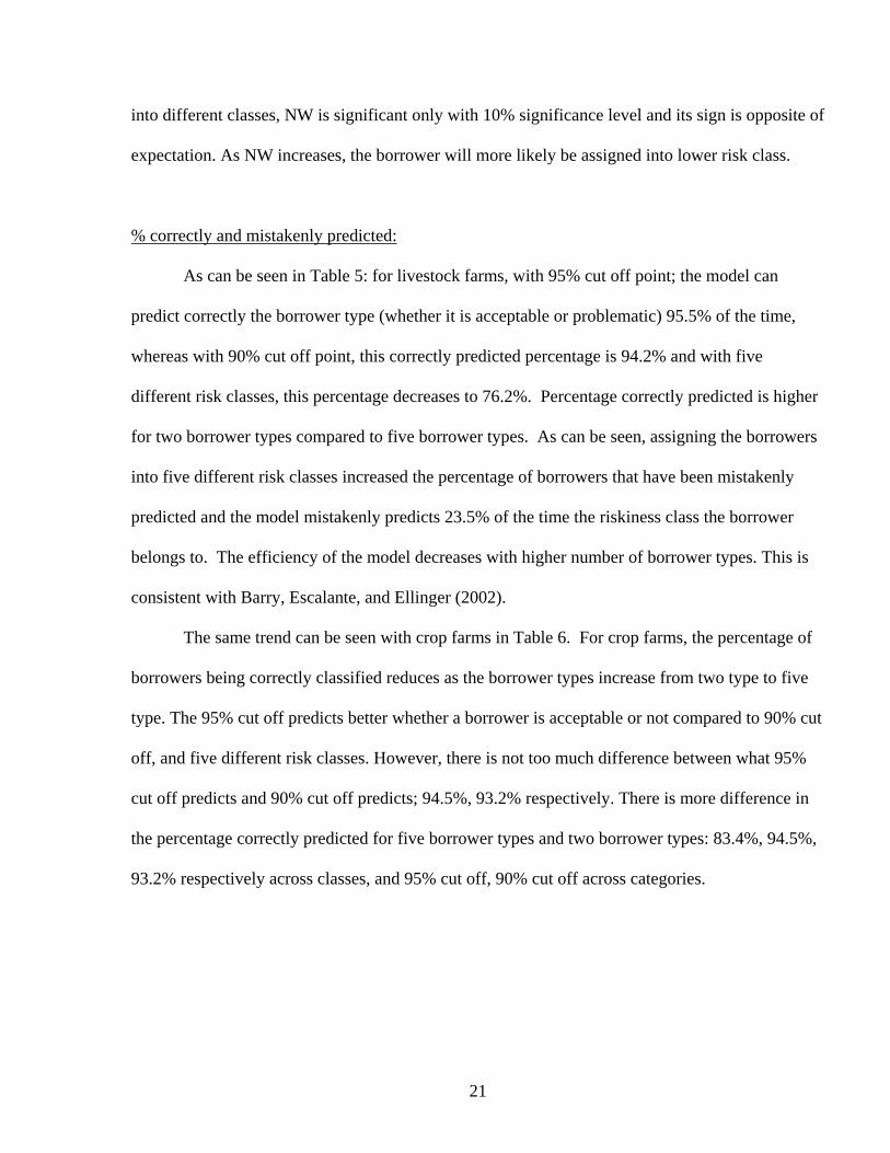
into different classes, NW is significant only with 10% significance level and its sign is opposite of

expectation. As NW increases, the borrower will more likely be assigned into lower risk class.

% correctly and mistakenly predicted:

As can be seen in Table 5: for livestock farms, with 95% cut off point; the model can

predict correctly the borrower type (whether it is acceptable or problematic) 95.5% of the time,

whereas with 90% cut off point, this correctly predicted percentage is 94.2% and with five

different risk classes, this percentage decreases to 76.2%. Percentage correctly predicted is higher

for two borrower types compared to five borrower types. As can be seen, assigning the borrowers

into five different risk classes increased the percentage of borrowers that have been mistakenly

predicted and the model mistakenly predicts 23.5% of the time the riskiness class the borrower

belongs to. The efficiency of the model decreases with higher number of borrower types. This is

consistent with Barry, Escalante, and Ellinger (2002).

The same trend can be seen with crop farms in Table 6. For crop farms, the percentage of

borrowers being correctly classified reduces as the borrower types increase from two type to five

type. The 95% cut off predicts better whether a borrower is acceptable or not compared to 90% cut

off, and five different risk classes. However, there is not too much difference between what 95%

cut off predicts and 90% cut off predicts; 94.5%, 93.2% respectively. There is more difference in

the percentage correctly predicted for five borrower types and two borrower types: 83.4%, 94.5%,

93.2% respectively across classes, and 95% cut off, 90% cut off across categories.

22

Significance of intercept:

For livestock farms; intercept is insignificant for 95% cut off across categories. This means

that there is no difference between borrower being acceptable or problematic with effects of

independent variable considered. The two categories are nearly the same. For 90% cut off across

categories, intercept is significant. Therefore, there is difference between borrowers being

acceptable or problematic even after controlling with several independent variables. The two

categories represent different borrower types. Across classes, all intercepts are significant. That

means lowest risk class is different than low risk class, low risk class is different than medium risk

class, medium risk class is different than high risk class and high risk class is different than highest

risk class. Different classes represent different borrower types.

For crop farms; 95% and 90% cut off across categories, intercept is significant. Therefore,

there is difference between borrower being acceptable or problematic. The two categories are not

the same. Across classes, all intercepts are significant. Different classes represent different

borrower types.

Summary and Conclusions

In conclusion, this article analyzed whether credit scoring models differ across livestock

farms and crop farms. As dependent variable, repayment capacity is used since it is an objective

way of measurement. Repayment capacity is measured by debt to farm operating income. This

dependent variable is categorized under 95% cut off, 90 % cut off, and across five credit risk

classes. The independent variables are tenure, liquidity, solvency, profitability, and financial

efficiency. These categories are measured by tenure, working capital to gross farm return

(WCGFR), net worth (NW), return on farm assets (ROFA), operating expense to gross farm return

23

(OEGFR) for crop farms or depreciation expense to gross farm return (DEGFR) for livestock

farms, and asset turnover ratio (ATR). Since, financial ratios are not normally distributed and

discriminant analysis assumes normal distribution; as statistical method LOGIT is used which has

the next highest prediction accuracy after discriminant analysis.

The following results are obtained for livestock farms and crop farms. For livestock farms;

liquidity, profitability, financial efficiency play significant role in assigning borrowers across

classes and categories, no matter what the cut off point is. However, solvency plays no significant

role to assign borrowers across categories or classes. The tenure ratio is sensitive to the cut off

point used for assigning borrowers into categories. With 90% cut off, tenure ratio is significant but

its sign is different than what is expected. Tenure ratio does not play any significant role to assign

borrowers into classes.

For crop farms; liquidity, profitability, financial efficiency, and tenure ratio all play

significant role in assigning borrowers across categories and classes. Solvency is also significantly

important while assigning borrowers across classes and categories.

When the borrower type is small (when borrower is categorized into two types either

acceptable or problematic), the model is predicted more accurately compared to higher number of

borrower type (five risk classes).

95% cut off better predicts the model compared to 90% cut off and five classes when we

look at percent concordant. However, for livestock farms; the 95% cut off fails in distinguishing

between acceptable borrower and problematic borrower when we look at the significance of

intercept.

24

A major conclusion drawn from these results is that multiple models are needed, separately

for livestock and crop farms, differing primarily in significance of the solvency and tenure

variables. Using the same model across multiple farm types would yield less accurate results.

To check for the robustness of this paper, the same model can be analyzed for different

number of classes such as three classes, seven classes etc. Further, this paper can be enhanced by

changing the way classes are created. Further, the same model can be applied to livestock farms

without including tenure while including tenure for crop farms, since tenure was added to see how

the sign of net worth changes for crop farms.

25

References

Barry P.J., C.L.Escalante, and P.N. Ellinger. “Credit Risk Migration Analysis of Farm

Businesses.” Agricultural Finance Review 62, (2002):1-11.

Boessen, C.R., A. Featherstone, L.N. Langemeier, and R.O. Burton. “Financial Performance of

Successful and Unsuccessful Farms.” Journal of the American Society of Farm Managers

and Rural Appraisers 54 (1990):6-15.

Escalante, C.L., P.J. Barry, T.A. Park, and E. Demir. “Farm-Level and Macroeconomic

Determinants of Farm Credit Risk Migration Rates.” Agricultural Finance Review 64

(2004): 135-149.

Featherstone, A.M., L.M. Roessler, and P.J. Barry. “Determining the Probability of Default and

Risk Rating Class for Loans in the Seventh Farm Credit District Portfolio.” Review of

Agricultural Economics 28 (2006):4-23.

Katchova, A.L., and P.J. Barry. “Credit Risk Models and Agricultural Lending.” American Journal

of Agricultural Economics 87 (2005): 194-205.

Lufburrow, J., P.J. Barry, and B.L. Dixon. “Credit Scoring for Farm Loan Pricing.” Agricultural

Finance Review 44 (1984): 8-14.

Miller, L.H., and E.L. LaDue. “Credit Assessment Models for Farm Borrowers: A Logit

Analysis.” Agricultural Finance Review 49 (1989): 22-36.

Nayak, G.N., and C.G. Turvey. “Credit Risk Assessment and the Opportunity Costs of Loan

Misclassification.” Canadian Journal of Agricultural Economics 45 (1997): 285-299.

Phillips, J.M., and A.L. Katchova. “Credit Score Migration Analysis of Farm Businesses:

Conditioning on Business Cycles and Migration Trends.” Agricultural Finance Review 64

(2004): 1-15.

26

Plumley, G.O., and R.H. Hornbaker. “Financial Management Characteristics of Successful Farm

Firms.” Agricultural Finance Review 51 (1991): 9-20.

Splett N.S., P.J.Barry, B.L.Dixon, and P.N.Ellinger. “A Joint Experience and Statistical Approach

to Credit Scoring.” Agricultural Finance Review 54 (1994):39-54.

Stephanou, C., and J.C. Mendoza. 2005. “Credit Risk Measurement Under Basel II: An Overview

and Implementation Issues for Developing Countries.” Policy Research Working Paper

Series 3556, The World Bank.

Turvey, C.G., and R. Brown. “Credit Scoring for a Federal Lending Institution: The Case of

Canada’s Farm Credit Corporation.” Agricultural Finance Review 50 (1990): 47-57.

Turvey, C.G. “Credit Scoring for Agricultural Loans: A Review with Applications.” Agricultural

Finance Review 51 (1991): 43-54.

27

Table 1. Variable Definitions and Expected Signs for Livestock Farms (Tenure Variable included)

Category Variable Definitions

Expected Sign in regards to Acceptable Borrower

Repayment Capacity

(DFOI) Debt to Farm Operating Income Debt / Farm Operating Income

Liquidity (WCGFR) Working Capital to Gross Farm Returns (Current Assets - Current Liabilities) / Gross Farm Returns (+)

Solvency (NW) Net Worth (market) Fair Market Value of Farm Assets - Fair Market Value of Farm Liabilities (-)

Profitability (ROFA) Return on Farm Assets (market)

(Net Farm Income from Operations + Farm Interest Payments - Unpaid Labor Charge for Operator and Family) / (Average Total Farm Assets in fair market value) (+)

Financial Efficiency

(DEGFR) Depreciation Expense to Gross Farm Return Total Farm Depreciation / Gross Farm Returns (-)

(ATR) Asset Turnover Ratio Value of Farm Production / Total Average Farm Assets (fair market value) (+)

Tenure (Tenure) Tenure Owned Acres / Total Acres Operated (-)

28

Table 2. Variable Definitions and Expected Signs for Crop Farms (Tenure Variable Included)

Category Variable Definitions

Expected Sign in regards to Acceptable Borrower

Repayment Capacity

(DFOI) Debt to Farm Operating Income Debt / Farm Operating Income

Liquidity (WCGFR) Working Capital to Gross Farm Returns (Current Assets - Current Liabilities) / Gross Farm Returns (+)

Solvency (NW) Net Worth (market) Fair Market Value of Farm Assets - Fair Market Value of Farm Liabilities (-)

Profitability (ROFA) Return on Farm Assets (market)

(Net Farm Income from Operations + Farm Interest Payments - Unpaid Labor Charge for Operator and Family) / (Average Total Farm Assets in fair market value) (+)

Financial Efficiency

(OEGFR) Operating Expense to Gross Farm Return (Total Operating Expenses - Depreciation) / Gross Farm Returns (-)

(ATR) Asset Turnover Ratio Value of Farm Production / Total Average Farm Assets (fair market value) (+)

Tenure (Tenure) Tenure Owned Acres / Total Acres Operated (-)

29

Table 3. Mean Values for Livestock Farms 95% cutoff in DFOI 90% cut off in DFOI Classes in DFOI

All Acceptable Borrower

Problematic Borrower

Acceptable Borrower

Problematic Borrower

Lowest Risk

Low Risk

Medium Risk

High Risk

Highest Risk

Debt to farm operating income 4.863 6.373 -0.199 5.149 4.100 0.692 2.839 6.080 16.674 99.343 Working capital to gross farm return 0.380 0.457 0.120 0.469 0.141 0.912 0.488 0.264 0.297 0.188 Net worth 820,670 844,171 741,907 842,240 763,239 1,047,591 846,256 722,267 838,141 802,864 Return on farm assets 0.054 0.080 -0.034 0.083 -0.024 0.092 0.102 0.080 0.037 0.017 Asset turnover ratio 0.318 0.340 0.243 0.346 0.242 0.345 0.368 0.370 0.254 0.290 Depreciation expense to gross farm return 0.093 0.075 0.155 0.073 0.146 0.083 0.060 0.068 0.098 0.136

Tenure ratio 0.363 0.357 0.381 0.358 0.376 0.345 0.350 0.352 0.387 0.393 Observations 879 677 202 639 240 122 210 200 145 49

Table 4. Mean Values for Crop Farms 95% Cut Off in DFOI 90% Cut Off in DFOI Classes in DFOI

All Acceptable Borrower

Problematic Borrower Acceptable

Borrower Problematic Borrower Lowest

Risk Low Risk

Medium Risk

High Risk

Highest Risk

Debt to farm operating income 4.126 6.730 -9.734 5.496 -1.053 0.770 2.844 6.187 16.226 128.292 Working capital to gross farm return 0.442 0.501 0.126 0.529 0.113 1.399 0.541 0.278 0.131 0.106 Net worth 821,714 832,391 764,887 838,904 756,721 1,097,219 839,635 738,984 762,718 813,630 Return on farm assets 0.052 0.066 -0.021 0.069 -0.012 0.075 0.093 0.063 0.031 0.007 Asset turnover ratio 0.345 0.355 0.288 0.359 0.290 0.323 0.394 0.363 0.318 0.279 Operating expense to gross farm return 0.631 0.601 0.788 0.596 0.762 0.554 0.569 0.611 0.660 0.710 Tenure ratio 0.239 0.234 0.263 0.232 0.265 0.274 0.214 0.212 0.260 0.306 Observations 7,530 6,339 1,191 5,955 1,575 1,019 1,893 1,902 1,526 374

30

Table 5. Logit Results for Livestock Farms Variables 95% Cut Offa 90% Cut Offb Classesc Intercept 1 -0.1289 -1.1167 -4.3495 (0.4676) (0.4302)** (0.3127)** Intercept 2 -2.4513 (0.2797)** Intercept 3 -0.8668 (0.2683)** Intercept 4 1.0918 (0.2875)** Working capital to gross farm return 2.022 1.96 2.0008 (0.2887)** (0.2632)** (0.1646)** Net worth -0.000000194 -0.000000225 -0.000000002 (2.377E-7) (2.11E-7) (1.247E-7) Return on farm assets 46.4815 40.8448 12.7758 (4.1478)** (3.4987)** (1.3781)** Depreciation expense to gross farm return -6.62 -4.8946 -2.6121 (1.7218)** (1.5705)** (1.0614)** Asset turnover ratio 2.617 3.1068 1.2412 (0.9203)** (0.8216)** (0.4507)** Tenure ratio 0.2543 0.7813 0.3906 (0.4919) (0.4511)* (0.2617) Number of observations 879 879 726 Log L (intercept only) -473.8185 -515.3195 -1,101.59 Likelihood Ratio (552.7853)** (556.7957)** (305.3367)** Score (382.9782)** (384.6812)** (238.5193)** Wald (148.9685)** (168.7452)** (260.1947)** Percent Concordant 95.5 94.2 76.2 Percent Discordant 4.4 5.7 23.5 Note: Standard errors are in parentheses and **, and * denote significance at 5% and 10%, respectively, and dependent variable is borrower being acceptable. Note:borrower=1 represents acceptable borrower, borrower=0 represents problematic borrower. aThe borrower is acceptable based on the 95% cut off. bThe borrower is acceptable based on the 90% cut off. cThe borrower is divided into 5 classes with 5 representing the highest risky class.

31

Table 6. Logit Results for Crop Farms Variables 95% Cut Offa 90% Cut Offb Classesc Intercept 1 6.8988 5.3721 -1.6195 (0.4023)** (0.3452)** (0.1849)** Intercept 2 0.7034 (0.1823)** Intercept 3 2.605 (0.1852)** Intercept 4 5.1362 (0.1959)** Working capital to gross farm return 1.4027 1.6755 2.3882 (0.0891)** (0.0860)** (0.0544)** Net worth -0.00000023 -0.000000137 6.762E-08 (6.957E-8)** (6.335E-8)** (4.026E-8)* Return on farm assets 36.2858 32.9085 13.871 (1.6264)** (1.3885)** (0.5650)** Operating expense to gross farm return -9.4895 -8.4501 -5.4182 (0.5440)** (0.4777)** (0.2736)** Asset turnover ratio 2.3441 2.1833 1.0752 (0.2703)** (0.2389)** (0.1296)** Tenure ratio -0.9159 -0.8432 -0.6009 (0.1898)** (0.1737)** (0.1134)** Number of observations 7,530 7,530 6,714 Log L (intercept only) -3,287.7365 -3,861.7310 -10,057.6005 Likelihood Ratio (3,468.3434)** (3,819.2782)** (4,527.8684)** Score (2,620.2321)** (2,771.5236)** (2,779.3175)** Wald (1,176.4132)** (1,376.3982)** (3,170.6801)** Percent Concordant 94.5 93.2 83.4 Percent Discordant 5.3 6.6 16.4 Note: Standard errors are in parentheses and **, and * denote significance at 5% and 10%, respectively, and dependent variable is borrower being acceptable. Note:borrower=1 represents acceptable borrower, borrower=0 represents problematic borrower. aThe borrower is acceptable based on the 95% cut off. bThe borrower is acceptable based on the 90% cut off. cThe borrower is divided into 5 classes with 5 representing the highest risky class.