General rights Copyright and moral rights for the publications made accessible in the public portal are retained by the authors and/or other copyright owners and it is a condition of accessing publications that users recognise and abide by the legal requirements associated with these rights.

Users may download and print one copy of any publication from the public portal for the purpose of private study or research.

You may not further distribute the material or use it for any profit-making activity or commercial gain

You may freely distribute the URL identifying the publication in the public portal If you believe that this document breaches copyright please contact us providing details, and we will remove access to the work immediately and investigate your claim.

Downloaded from orbit.dtu.dk on: Feb 15, 2022

Creating geometrically robust designs for highly sensitive problems using topologyoptimization: Acoustic cavity design

Christiansen, Rasmus E.; Lazarov, Boyan S.; Jensen, Jakob S.; Sigmund, Ole

Published in:Structural and Multidisciplinary Optimization

Link to article, DOI:10.1007/s00158-015-1265-5

Publication date:2015

Document VersionPeer reviewed version

Link back to DTU Orbit

Citation (APA):Christiansen, R. E., Lazarov, B. S., Jensen, J. S., & Sigmund, O. (2015). Creating geometrically robust designsfor highly sensitive problems using topology optimization: Acoustic cavity design. Structural and MultidisciplinaryOptimization, 52(4), 737-754. https://doi.org/10.1007/s00158-015-1265-5

Noname manuscript No.(will be inserted by the editor)

Creating Geometrically Robust Designs for Highly Sensitive Problemsusing Topology OptimizationAcoustic Cavity Design

Rasmus E. Christiansen, Boyan S. Lazarov, Jakob S. Jensen, Ole Sigmund.

Received: date / Accepted: date

Abstract Resonance and wave-propagation problems areknown to be highly sensitive towards parameter variations.This paper discusses topology optimization formulationsfor creating designs that perform robustly under spatialvariations for acoustic cavity problems. For several struc-tural problems, robust topology optimization methods havealready proven their worth. However, it is shown thatdirect application of such methods is not suitable for theacoustic problem under consideration. A new double filterapproach is suggested which makes robust optimizationfor spatial variations possible. Its effect and limitationsare discussed. In addition, a known explicit penalizationapproach is considered for comparison. For near-uniformspatial variations it is shown that highly robust designscan be obtained using the double filter approach. It isfinally demonstrated that taking non-uniform variations intoaccount further improves the robustness of the designs.

Keywords topology optimization· robust design· wavepropagation· acoustics· noise reduction· projectionfiltering · uniform design variations· non-uniform designvariations

1 Introduction

It is widely known that solutions to interior acousticproblems in the medium to high frequency range are highly

R. E. Christiansen (*)· B. S. Lazarov· O. SigmundDepartment of Mechanical Engineering, Solid Mechanics,Technical University of Denmark, Nils Koppels Alle, B. 404,DK-2800 Lyngby, DenmarkE-mail: (*) raelch@mek.dtu.dk

J. S. JensenDepartment of Electrical Engineering,Centre for Acoustic-Mechanical Micro SystemsTechnical University of Denmark, Ørsteds Plads, B. 352,DK-2800 Lyngby, Denmark.

sensitive to parameter variations (Jacobsen and Juhl, 2013).For high frequencies the problems are so sensitive thatonly statistical methods are viable, e.g. statistical energyanalysis (Lyon and DeJONG, 1998). In this paper we areinterested in deterministic solutions for the pressure fieldand thus restrict ourselves to the low/medium frequencyrange. We consider a 2D interior acoustics problem withreflecting boundaries for single frequencies. We seek tominimize the sound pressure in part of the domain utilizinginterference phenomena by placing material in the domainusing topology optimization (Bendsøe and Sigmund, 2003).We base our approach on the work by Duhring et al (2008)where the topology optimization formulation for interioracoustic problems was presented. It was shown to bepossible to significantly reduce the sound pressure in adesignated part of the domain by placing material elsewhere.We demonstrate that the pressure field is very sensitiveto variations in the geometry of the optimized designeven at medium frequencies. This is problematic from anapplication point of view since it is likely impossible tomanufacture or install the designs exactly to specifications,leaving the designs useless in real world applications.

We present a topology optimization based approach forcreating designs that maintain high performance undersubstantial near-uniform and small non-uniform geometricvariations. For problems in structural mechanics, heatconduction (Wang et al, 2011b), and optics (Wang et al,2011a; Elesin et al, 2012), it has been shown that usinga robust optimization approach leads to a significantimprovement in the robustness of the design’s perfor-mance under spatial variations. We base our approachon the work by Wang et al (2011b). Here the designis optimized for a nominal, an eroded and a dilatedrealization simultaneously using a min/max formulation.The realizations are obtained using continuous projectionof

2

smoothed design variables. We demonstrate that applyingthe robust scheme directly is insufficient for the presentacoustic problem due to unpredictable variations in theeroded and dilated designs, making it impossible to performmeaningful robust optimization. To alleviate the problemwe present a double filter which restricts design featuresto vary along their edges as the projection level changes.This allows for optimization of designs towards geometricvariations. Promising results for designs optimized underboth near-uniform and non-uniform geometric variationsare presented. A related double filter approach developedindependently of the approach presented in this paperis used in a structural mechanics topology optimizationformulation for creating coated structures (Clausen et al,Submitted). Other papers have treated and demonstratedthe usefulness of topology optimization for problems inacoustics e.g. Wadbro and Berggren (2006); Lee and Kim(2009); Kook et al (2012); Wadbro (2014) and acousticstructure interaction, e.g. Yoon et al (2007); Du and Olhoff(2007). The question of geometric robustness of thedesigns have, to our knowledge, not been investigatedelsewhere. As a final note it is stressed that the optimizationproblems considered here are highly non-convex. Hencesmall changes in problem or optimization parameters maylead the optimization procedure to converge to differentrobust designs.

2 Model Problem

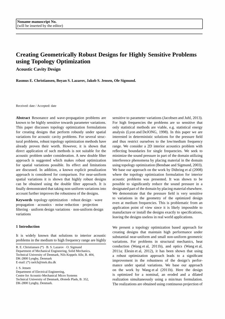
We seek to minimize the square of the average soundpressure amplitude,|p|2, in the sub-domainΩOP of themodel domainΩ ⊂ R

2. A small source domainP is usedto excite acoustic waves. The reduction in|p|2 is achievedby introducing solid material in a regionΩd replacing theacoustic medium.ΩOP, Ωd and P are sub-domains ofΩand are assumed to be non-intersecting. The boundary ofΩ, denotedδΩ, is taken to be perfectly reflecting. Figure1 shows the domain configuration used, unless otherwisenoted.

Fig. 1: Illustration of the domain configuration.Ω = [0, 18] × [0, 9]ΩOP = [15, 17]×[1, 3] is the optimization domain,Ωd = [0, 18]×[8, 9]is the design domain andP = [1.9, 2.1]× [1.9, 2.1] denotes the regionwhere an acoustic wave is exited.

3 Physics Model

Time-harmonic acoustic wave-propagation in an adiabaticmedium is governed by the Helmholtz equation,

∇ · (ρ(x)−1∇p(x)) + ω2κ(x)−1p(x) = 0, x ∈ Ω. (1)

Here ∇ denotes the spatial derivative,p is the complexsound pressure andρ andκ are the density and bulk modulusof the medium, respectively.ω = 2πf is the angularfrequency wheref is denoted the excitation frequency. Thespatial dependence in (1) is suppressed in the following forbrevity. The perfectly reflecting boundaries and the sourceare imposed using,

n · (ρ−1∇p) = 0, ∀ x ∈ δΩ, (2)

n · (ρ−1∇p) = −iωU, ∀ x ∈ δP. (3)

Here n is the outward pointing normal vector to theboundary in question andU is the vibrational velocity.

The material parameters of solid and air are chosen to have avery large contrast between them. This justifies disregardingthe structural problem of the solid material as it will simplyact as hard wall boundary conditions for the acoustic waves.The material parameters have been chosen to match thosefor atmospheric air and aluminum given by,

air: ρ1 = 1.204 kg m−3, κ1 = 141.921 · 103 N m−2. (4)

Al: ρ2 = 2643.0 kg m−3, κ2 = 6.87 · 1010 N m−2. (5)

We perform a rescaling of the parameters in the model,

3

(ρ, κ) =

(1, 1) air(

ρ2

ρ1

, κ2

κ1

)

solid, ω =

ω

c, c =

√

κ1

ρ1, (6)

wherec is the speed of sound in the gas (acoustic medium).By applying the rescaling (1), (2) and (3) becomes,

∇ · (ρ−1∇p) + ω2κ−1p = 0, x ∈ Ω, (7)

n · (ρ−1∇p) = 0, ∀ x ∈ δΩ, (8)

n · (ρ−1∇p) = −iωU√κ1ρ1, ∀ x ∈ δP. (9)

All results are reported using the sound pressure level,abbreviated SPL, for a given,p, which is calculated as,

Lp = 10 log10

( |p|2pref

2

)

, pref,air = 20 µPa. (10)

pref is the material dependent reference pressure for air,(Jacobsen and Juhl, 2013).

4 The Optimization Problem

Minimizing the average of|p|2 over ΩOP, is equivalentto minimizing the average ofLp over ΩOP, henceforthdenoted〈Lp〉ΩOP. The discrete problem of placing materialin Ωd is replaced by a continuous problem, see Duhring et al(2008). A design variable field,0 ≤ ξ(x) ≤ 1, ∀ x ∈Ωd, ξ(x) = 0 ∀ x ∈ Ω\Ωd, is introduced and a linearinterpolation of the inverse density and bulk modulus isused. This interpolation is given by,

ρ(ξ)−1 = 1 + ξ

(

(

ρ2ρ1

)−1

− 1

)

, (11)

κ(ξ)−1 = 1 + ξ

(

(

κ2

κ1

)−1

− 1

)

. (12)

The optimization problem may be stated as,

minξ

. : Φ =1

AOP

∫

|p(ξ)|2dΩOP, AOP =

∫

dΩOP, (13)

s.t. : 0 ≤ ξ(x) ≤ 1 ∀ x ∈ Ωd,

HereΦ denotes the objective.p(ξ) is obtained by solving(7)-(9) for a given design variable field,ξ(x). Solving (13)using the approach outlined in sections 4-6 is in the rest ofthe paper denoted asthe standard approach.

5 The Discrete Problem

The domainΩ, governing PDE (7) and correspondingboundary conditions (8)-(9) are discretized using the finiteelement method (FEM). For the discretization Q4 elementsof equal size are used throughoutΩ with a total ofN nodesin the mesh. The linear basis function connected to nodekis denotedNk. The discretization yields the linear system,

Sp = (K(ρ)− ω2M(κ))p = F. (14)

F stems from the boundary condition (9), and is given as,

Fk =∑

i∈Nb,k

∫

δΩi

n · (ρ−1∇p)NkdΩ (15)

HereNb,k denotes the boundary edges connected to nodek.K andM in (14) are given by,

Kij =

∫

ρ−1∇Ni∇NjdΩ, Mij =

∫

κ−1NiNjdΩ, (16)

wherei ∈ 1, 2, ...,N, j ∈ 1, 2, ...,N. NeitherM norK needs modifications to take the boundary conditions intoaccount. The solution to (7),p, is approximated by,

p ≈∑

k∈N

pkNk, (17)

wherepk is the k’th entry inp, the solution of (14).

The design variable field,ξ(x), is discretized in adiscontinuous manner using piecewise constant values ineach finite element.

5.1 Sensitivities

The sensitivities required for the topology optimizationprocedure are obtained using adjoint sensitivity analysis, seeDuhring et al (2008) and references therein. They are,

dΦdξi

=∂Φ

∂ξi+ ℜ

(

λT ∂S∂ξi

p)

. (18)

Hereℜ denotes the real part, T denotes the transpose andλ

is obtained by solving,

STλ = −(

∂Φ

∂pR

− i∂Φ

∂pI

)T

, p = pR + ipI , (19)

with thek’th entry in the right hand side given as,

(

∂Φ

∂pR

− i∂Φ

∂pI

)

k

=1

AOP

∫

2(pR − ipI)NkdΩOP. (20)

4

6 Filtering and Projection Strategy

A density filter is used for smoothing followed by aprojection to ensure a 0/1-design, (Guest et al, 2004;Xu et al, 2010; Wang et al, 2011b). In the following· isused to denote smoothed variables and· denotes projectedvariables. When multiple operations are applied to a variablethe symbols are ordered with the latest operation on top.Equation (21) presents the discretized version of the applieddensity filter (Bourdin, 2001; Bruns and Tortorelli, 2001),

ξi =

∑

j∈Be,iw(xi − xj)Ajξj

∑

j∈Be,iw(xi − xj)Aj

. (21)

Aj is the area of thej’th element,Be,i denotes the designvariables which are within a given filter radiusR of designvariablei. Herexj is taken to be the average of the nodalpositions in elementj. The filter functionw is given by,

w(x) =

R− |x| ∀ |x| ≤ R ∧ x ∈ Ωd

0 otherwise, (22)

whereR is the aforementioned filter radius. To allow thedesign to vary with projection level along the edge ofΩd

facing into the domain an extended filter area reachingoutside ofΩd was used. In the extended filter area thedesign variables are all identically zero. A dashed line isincluded on all designs presented in figures to denote theedge ofΩd.

The projection operator used is the one suggested byWang et al (2011b) and is given as,

ξi =tanh(βη) + tanh(β(ξi − η))

tanh(βη) + tanh(β(1 − η)), (23)

whereβ is a parameter used to control the sharpness ofthe projection andη ∈ [ξmin, ξmax] defines the projectionlevel. η = 0.5 has been used as the target for thefinal (nominal) designs in all cases. When applying thedensity filter and projection the pressure field will dependexplicitly on the filtered and projected variables,¯

ξ. Hencethe optimization problem (13) and the sensitivities shouldbe modified accordingly.

6.1 Modification of Sensitivities

Applying the smoothing (21) and projection (23) operationson ξ requires the following sensitivity modifications,

dΦdξi

=∑

h∈Be,i

∂ξh∂ξi

∂ ¯ξh

∂ξh

dΦ

d¯ξh, (24)

with,

∂ξh∂ξi

=w(xh − xi)Ai

∑

j∈Ne,hw(xh − xj)Aj

, (25)

∂¯ξh

∂ξh=

β sech2(β(ξh(x)− η))

tanh(βη) + tanh(β(1 − η)), (26)

and dΦd¯ξh

given by (18).

6.2 β-Continuation Scheme

The projection step is used together with a continuationscheme forβ, see Guest et al (2004), which graduallyincreases the projection strength during the optimizationprocess. This scheme prevents that the optimization getsstuck prematurely in a local minimum during the firstiterations due to the design being projected to 0/1immediately. A more conservative scheme than the onesuggested by Wang et al (2011b) is used here, see algorithm1. In the present schemeβ is only increased ifΦ has notchanged significantly fornsc iterations.

Algorithm 1 β continuation scheme.

1: Current objective:Φc, Previousnsc objectives:Φnsc.2: if (nsc or more iterations have occurred since lastβ increase.)then3: if |Φc −max(Φnsc)| < α|Φc| then4: β = 1.2 · β.5: end if6: end if7: return β

7 Implementation, Validation and Parameter Choices

MATLAB was used for the implementation and the mini-mization problems were solved using the Method of MovingAsymptotes, MMA (Svanberg, 1987). The MATLAB solverwas validated using the method of manufactured solutionsand through comparison with COMSOL MULTIPHYSICSVersion 4.3b’s acoustics module. COMSOL was also usedto validate the performance of selected final designs.Table 1 lists the parameter values which have been used inall numerical experiments unless stated otherwise.

8 Sample Solution

An example of the effect on the pressure field of placing anoptimized design inΩd is presented here. Figure 2i showstheLp-field for the excitation frequencyf = 51.32 Hz inan empty domain. Figure 2ii shows theLp-field in the samedomain after a design optimized for this frequency using thestandard approach is introduced. It is clearly seen that the

5

Table 1: Parameters used in simulations.Nx,Ny: numberof elements in thex− andy− direction.ξini : initial designvariable value.R: filter radius. U : vibrational velocity.βini , βmax: initial and finalβ-value.nsc: minimum iterationsbetween β increases.α: objective variation parameter.x•, y•: spatial extend of the domain•.

Parameter [Unit] Value

Nx [elements] 720

Ny [elements] 360

ξini ∀ x ∈ Ωd 0.15

R [elements] 20

U [ms ] 0.01

βinit 1

βmax 500

nsc 10

α 0.01

xΩ [m]× yΩ [m] [0, 18]× [0, 9]

xΩd [m]× yΩd [m] [0, 18]× [8, 9]

xΩOP [m]× yΩOP [m] [15, 17]× [1, 3]

xP [m]× yP [m] [1.9, 2.1]× [1.9, 2.1]

minimization ofLp in ΩOP is achieved by a combinationof two mechanisms. First a reduction of the overall soundpressure inΩ from a maximum of 112 dB to 95 dB hasoccurred and secondly nodal lines have been moved intoΩOP leading to a significant reduction of the average soundpressure level inΩOP, 〈Lp〉ΩOP.

x [m]

y[m

]

0 2 4 6 8 10 12 14 16 18

9876543210

0

20

40

60

80

100

(i) Lp in empty model domain.

x [m]

y[m

]

0 2 4 6 8 10 12 14 16 18

9876543210

−20

0

20

40

60

80

(ii) Lp in model domain where optimized design has been introduced.

Fig. 2: Pressure fields measured usingLp at the excitation frequencyf = 51.32 Hz. The acoustic source andΩOP are outlined using thinblack lines.

〈Lp〉ΩOP, has been reduced from approximately103 dBfor the empty domain to approximately38.8 dB whenthe optimized design is introduced. An important notehere is that the magnitude of the reduction in〈Lp〉ΩOP

clearly depends on how the nodal lines of the field in theempty room line up withΩOP. In the present examplea larger magnitude of the reduction could possibly havebeen obtained by movingΩOP to [13.5, 15.5] × [1.3]. Themagnitude of the reduction is not the main interest ofthis study however. The fact that a significant reduction insound pressure may be obtained by introducing the designis of course important. It is however the robustness of thisreduction towards variations in the design which is theconcern in the following.

9 Intermediate Design Variables

In order for the final designs to be meaningful for real worldapplication they must consist of design variables taking thevalues 0 or 1, corresponding to no material or material ateach position in space. The projection operator presentedin (23) enforces a 0/1 design by projecting at the thresholdvalueη ∈ [ηmin, ηmax], ηmin ∈ [0, ηmax[, ηmax ∈ ]ηmax, 1].As described in the introduction it is possible to use avarying projection level,η, to optimize the design towardsworst case spatial variations. However, as will be shownin the following there is no guarantee that this approachresults in an appropriately varying design. In this contextappropriately should be understood as follows: Firstly,

6

a)

b)

c)

d)

0

0.2

0.4

0.6

0.8

1

(i) Smoothed design variables,ξ(x).

a)

b)

c)

d)

(ii) Final designs. (Physical design variables,¯ξ(x) projected atη =

0.5).

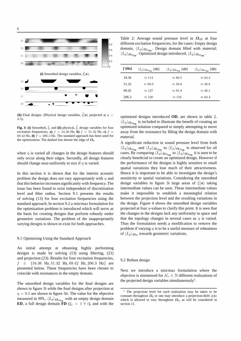
Fig. 3: (i) Smoothed,ξ, and(ii) physical, ¯ξ, design variables for fourexcitation frequencies,a) f = 34.36 Hz, b) f = 51.32 Hz, c) f =69.42 Hz, d) f = 206.3 Hz. The standard approach has been used forthe optimization. The dashed line denote the edge ofΩd.

whenη is varied all changes in the design features shouldonly occur along their edges. Secondly, all design featuresshould change near-uniformly in size ifη is varied.

In this section it is shown that for the interior acousticproblem the design does not vary appropriately withη andthat this behavior increases significantly with frequency.Theissue has been found to exist independent of discretizationlevel and filter radius. Section 9.1 presents the resultsof solving (13) for four excitation frequencies using thestandard approach. In section 9.2 a min/max formulation forthe optimization problem is introduced which will serve asthe basis for creating designs that perform robustly undergeometric variations. The problem of the inappropriatelyvarying designs is shown to exist for both approaches.

9.1 Optimizing Using the Standard Approach

An initial attempt at obtaining highly performingdesigns is made by solving (13) using filtering, (21)and projection (23). Results for four excitation frequencies,f ∈ 34.36 Hz, 51.32 Hz, 69.42 Hz, 206.3 Hz arepresented below. These frequencies have been chosen tocoincide with resonances in the empty domain.

The smoothed design variables for the final designs areshown in figure 3i while the final designs after projection atη = 0.5 are shown in figure 3ii. The value for the objectivemeasured in SPL,〈Lp〉ΩOPXX

with an empty design domainED, a full design domainFD (ξi = 1 ∀ i), and with the

Table 2: Average sound pressure level inΩOP at fourdifferent excitation frequencies, for the cases: Empty designdomain, 〈Lp〉ΩOPED

. Design domain filled with material;〈Lp〉ΩOPFD

. Optimized design introduced,〈Lp〉ΩOPOD.

f [Hz] 〈Lp〉ΩOPED[dB] 〈Lp〉ΩOPFD

[dB] 〈Lp〉ΩOPOD[dB]

34.36 ≈ 114 ≈ 80.5 ≈ 64.4

51.32 ≈ 99.0 ≈ 59.0 ≈ 38.8

69.42 ≈ 127 ≈ 91.8 ≈ 46.1

206.3 ≈ 120 ≈ 116 ≈ 64.4

optimized designs introducedOD, are shown in table 2.〈Lp〉ΩOPFD

is included to illustrate the benefit of creating anoptimized solution compared to simply attempting to moveaway from the resonance by filling the design domain withmaterial.

A significant reduction in sound pressure level from both〈Lp〉ΩOPED

and 〈Lp〉ΩOPFDto 〈Lp〉ΩOPOD

is observed for allcases. By comparing〈Lp〉ΩOPOD

to 〈Lp〉ΩOPFDit is seen to be

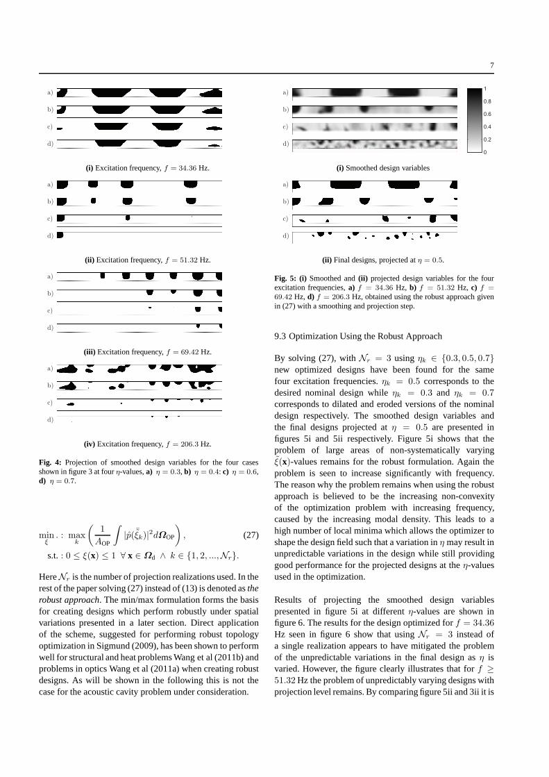
clearly beneficial to create an optimized design. However ifthe performance of the designs is highly sensitive to smallspatial variations they lose much of their attractiveness.Hence it is important to be able to investigate the design’ssensitivity to spatial variations. Considering the smootheddesign variables in figure 3i large areas ofξ(x) takingintermediate values can be seen. These intermediate valuesmake it impossible to establish a meaningful relationbetween the projection level and the resulting variations inthe design. Figure 4 shows the smoothed design variablesprojected at fourη-values to clarify this point. It is seen thatthe changes in the designs lack any uniformity in space andthat the topology changes in several cases asη is varied.Thus the formulation needs a modification to remove theproblem if varyingη is to be a useful measure of robustnessof 〈Lp〉ΩOP towards geometric variations.

9.2 Robust design

Next we introduce a min/max formulation where theobjective is minimized forNr ∈ N different realizations ofthe projected design variables simultaneously1.

1 The projection level for each realization may be taken to beconstant throughoutΩd or one may introduce a projection-fieldη(x)which is allowed to vary throughoutΩd, as will be considered insection 11.

7

a)

b)

c)

d)

(i) Excitation frequency,f = 34.36 Hz.

a)

b)

c)

d)

(ii) Excitation frequency,f = 51.32 Hz.

a)

b)

c)

d)

(iii) Excitation frequency,f = 69.42 Hz.

a)

b)

c)

d)

(iv) Excitation frequency,f = 206.3 Hz.

Fig. 4: Projection of smoothed design variables for the four casesshown in figure 3 at fourη-values,a) η = 0.3, b) η = 0.4: c) η = 0.6,d) η = 0.7.

minξ

. : maxk

(

1

AOP

∫

|p( ¯ξk)|2dΩOP

)

, (27)

s.t. : 0 ≤ ξ(x) ≤ 1 ∀ x ∈ Ωd ∧ k ∈ 1, 2, ...,Nr.

HereNr is the number of projection realizations used. In therest of the paper solving (27) instead of (13) is denoted astherobust approach. The min/max formulation forms the basisfor creating designs which perform robustly under spatialvariations presented in a later section. Direct applicationof the scheme, suggested for performing robust topologyoptimization in Sigmund (2009), has been shown to performwell for structural and heat problems Wang et al (2011b) andproblems in optics Wang et al (2011a) when creating robustdesigns. As will be shown in the following this is not thecase for the acoustic cavity problem under consideration.

a)

b)

c)

d)

0

0.2

0.4

0.6

0.8

1

(i) Smoothed design variables

a)

b)

c)

d)

(ii) Final designs, projected atη = 0.5.

Fig. 5: (i) Smoothed and(ii) projected design variables for the fourexcitation frequencies,a) f = 34.36 Hz, b) f = 51.32 Hz, c) f =69.42 Hz, d) f = 206.3 Hz, obtained using the robust approach givenin (27) with a smoothing and projection step.

9.3 Optimization Using the Robust Approach

By solving (27), withNr = 3 usingηk ∈ 0.3, 0.5, 0.7new optimized designs have been found for the samefour excitation frequencies.ηk = 0.5 corresponds to thedesired nominal design whileηk = 0.3 and ηk = 0.7corresponds to dilated and eroded versions of the nominaldesign respectively. The smoothed design variables andthe final designs projected atη = 0.5 are presented infigures 5i and 5ii respectively. Figure 5i shows that theproblem of large areas of non-systematically varyingξ(x)-values remains for the robust formulation. Again theproblem is seen to increase significantly with frequency.The reason why the problem remains when using the robustapproach is believed to be the increasing non-convexityof the optimization problem with increasing frequency,caused by the increasing modal density. This leads to ahigh number of local minima which allows the optimizer toshape the design field such that a variation inη may result inunpredictable variations in the design while still providinggood performance for the projected designs at theη-valuesused in the optimization.

Results of projecting the smoothed design variablespresented in figure 5i at differentη-values are shown infigure 6. The results for the design optimized forf = 34.36

Hz seen in figure 6 show that usingNr = 3 instead ofa single realization appears to have mitigated the problemof the unpredictable variations in the final design asη isvaried. However, the figure clearly illustrates that forf ≥51.32 Hz the problem of unpredictably varying designs withprojection level remains. By comparing figure 5ii and 3ii it is

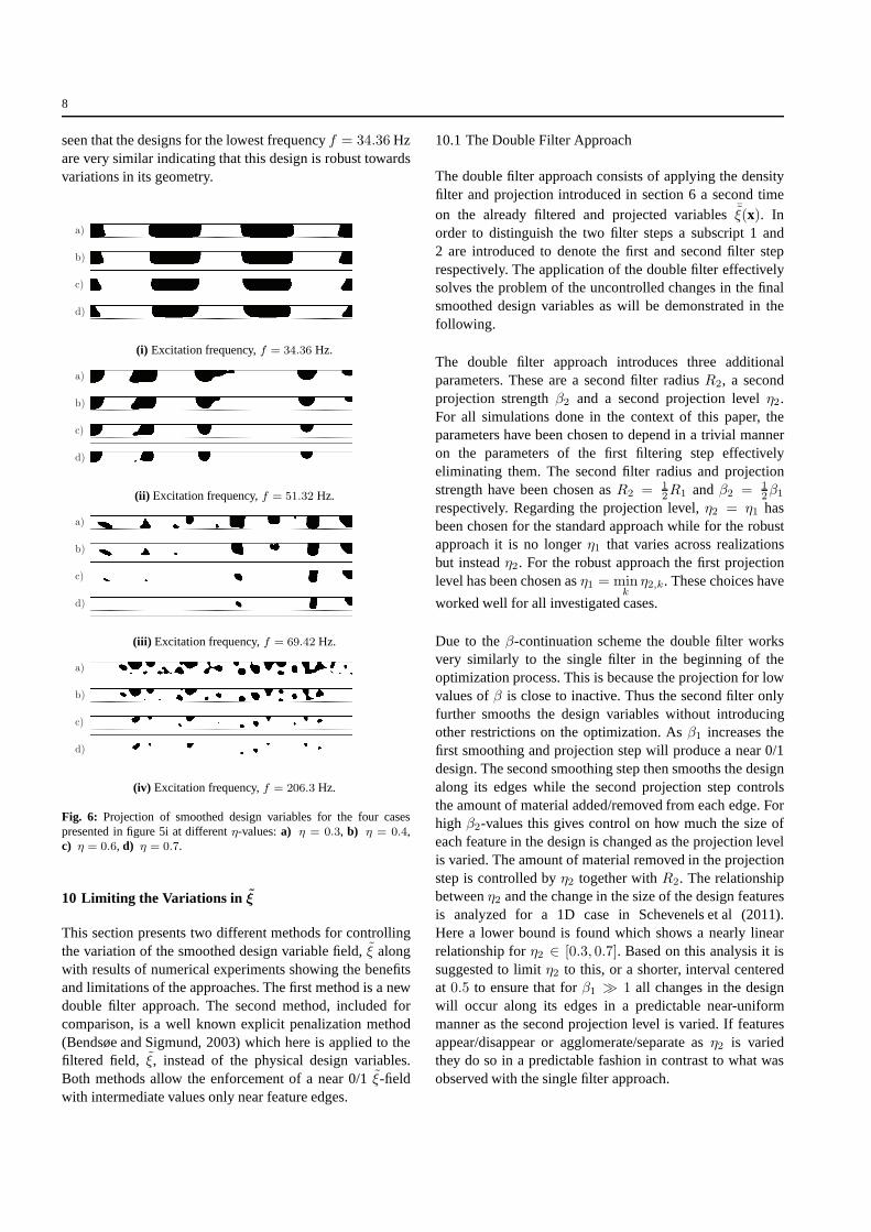
8

seen that the designs for the lowest frequencyf = 34.36 Hzare very similar indicating that this design is robust towardsvariations in its geometry.

a)

b)

c)

d)

(i) Excitation frequency,f = 34.36 Hz.

a)

b)

c)

d)

(ii) Excitation frequency,f = 51.32 Hz.

a)

b)

c)

d)

(iii) Excitation frequency,f = 69.42 Hz.

a)

b)

c)

d)

(iv) Excitation frequency,f = 206.3 Hz.

Fig. 6: Projection of smoothed design variables for the four casespresented in figure 5i at differentη-values:a) η = 0.3, b) η = 0.4,c) η = 0.6, d) η = 0.7.

10 Limiting the Variations in ξ

This section presents two different methods for controllingthe variation of the smoothed design variable field,ξ alongwith results of numerical experiments showing the benefitsand limitations of the approaches. The first method is a newdouble filter approach. The second method, included forcomparison, is a well known explicit penalization method(Bendsøe and Sigmund, 2003) which here is applied to thefiltered field, ξ, instead of the physical design variables.Both methods allow the enforcement of a near 0/1ξ-fieldwith intermediate values only near feature edges.

10.1 The Double Filter Approach

The double filter approach consists of applying the densityfilter and projection introduced in section 6 a second timeon the already filtered and projected variables¯ξ(x). Inorder to distinguish the two filter steps a subscript 1 and2 are introduced to denote the first and second filter steprespectively. The application of the double filter effectivelysolves the problem of the uncontrolled changes in the finalsmoothed design variables as will be demonstrated in thefollowing.

The double filter approach introduces three additionalparameters. These are a second filter radiusR2, a secondprojection strengthβ2 and a second projection levelη2.For all simulations done in the context of this paper, theparameters have been chosen to depend in a trivial manneron the parameters of the first filtering step effectivelyeliminating them. The second filter radius and projectionstrength have been chosen asR2 = 1

2R1 andβ2 = 1

2β1

respectively. Regarding the projection level,η2 = η1 hasbeen chosen for the standard approach while for the robustapproach it is no longerη1 that varies across realizationsbut insteadη2. For the robust approach the first projectionlevel has been chosen asη1 = min

kη2,k. These choices have

worked well for all investigated cases.

Due to theβ-continuation scheme the double filter worksvery similarly to the single filter in the beginning of theoptimization process. This is because the projection for lowvalues ofβ is close to inactive. Thus the second filter onlyfurther smooths the design variables without introducingother restrictions on the optimization. Asβ1 increases thefirst smoothing and projection step will produce a near 0/1design. The second smoothing step then smooths the designalong its edges while the second projection step controlsthe amount of material added/removed from each edge. Forhigh β2-values this gives control on how much the size ofeach feature in the design is changed as the projection levelis varied. The amount of material removed in the projectionstep is controlled byη2 together withR2. The relationshipbetweenη2 and the change in the size of the design featuresis analyzed for a 1D case in Schevenels et al (2011).Here a lower bound is found which shows a nearly linearrelationship forη2 ∈ [0.3, 0.7]. Based on this analysis it issuggested to limitη2 to this, or a shorter, interval centeredat 0.5 to ensure that forβ1 ≫ 1 all changes in the designwill occur along its edges in a predictable near-uniformmanner as the second projection level is varied. If featuresappear/disappear or agglomerate/separate asη2 is variedthey do so in a predictable fashion in contrast to what wasobserved with the single filter approach.

9

The choice ofR2 relative toR1 is important. IfR2 is chosentoo large compared toR1 the functionality of the doublefilter is lost for the following reason. The first smoothingoperation creates a functional dependence between designvariables which are less thanR1 apart. Thus the field¯ξmay in some sense be seen as a coarser version of theoriginal design field. Filtering a second time with a largeradiusR2 can therefore be seen as functionally equivalentto smoothing only a single time on the unfiltered designvariables. Thus unpredictable variations in the design withprojection level may be observed ifR2 is chosen to large.From our experimentation for the acoustic cavity problem ithas been found that choosingR2 such thatR2 ≤ R1

2works

well for all investigated cases. ChoosingR2 ≥ R1 has beenfound to destroy the effect of the double filter in severalcases.

The choice ofβ2 controls the sharpness of the secondprojection. Just as for the single filter, ifβ2 is chosen with tohigh initial value, it will force the optimizer to converge to asuboptimal local minimum since the design variable field isforced immediately towards 0/1.

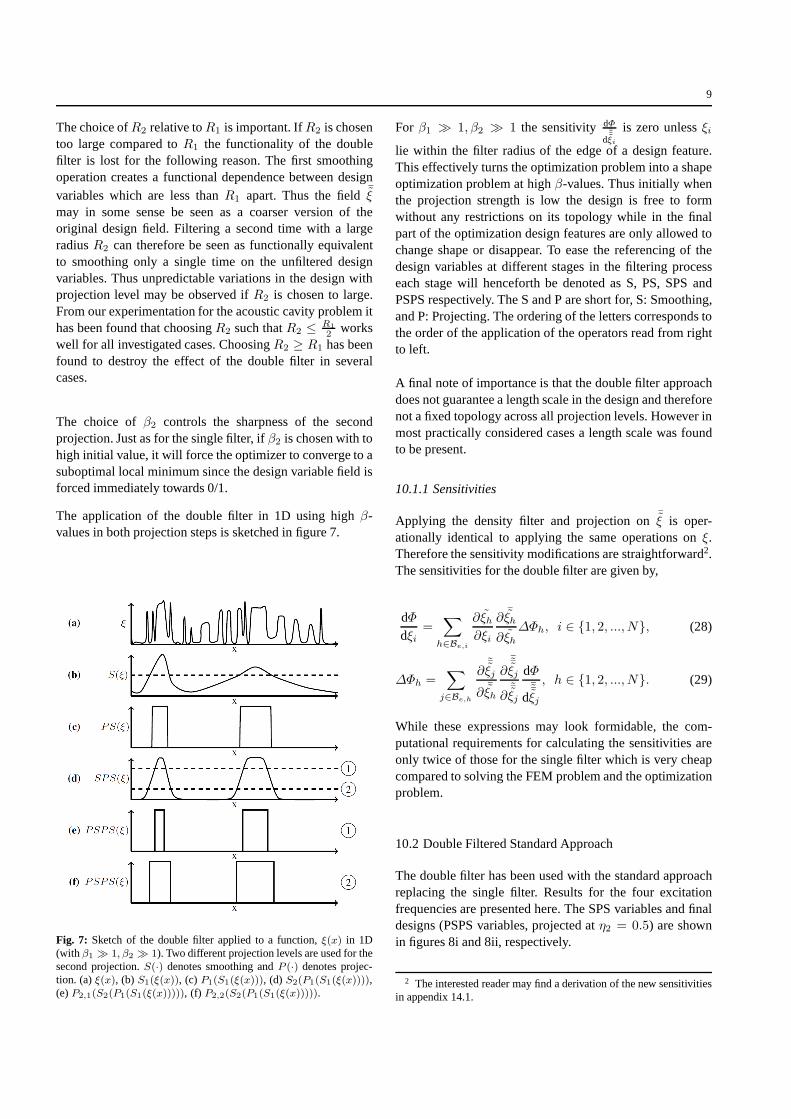
The application of the double filter in 1D using highβ-values in both projection steps is sketched in figure 7.

Fig. 7: Sketch of the double filter applied to a function,ξ(x) in 1D(with β1 ≫ 1, β2 ≫ 1). Two different projection levels are used for thesecond projection.S(·) denotes smoothing andP (·) denotes projec-tion. (a)ξ(x), (b) S1(ξ(x)), (c) P1(S1(ξ(x))), (d) S2(P1(S1(ξ(x)))),(e)P2,1(S2(P1(S1(ξ(x))))), (f) P2,2(S2(P1(S1(ξ(x))))).

For β1 ≫ 1, β2 ≫ 1 the sensitivity dΦ

d¯¯ξi

is zero unlessξi

lie within the filter radius of the edge of a design feature.This effectively turns the optimization problem into a shapeoptimization problem at highβ-values. Thus initially whenthe projection strength is low the design is free to formwithout any restrictions on its topology while in the finalpart of the optimization design features are only allowed tochange shape or disappear. To ease the referencing of thedesign variables at different stages in the filtering processeach stage will henceforth be denoted as S, PS, SPS andPSPS respectively. The S and P are short for, S: Smoothing,and P: Projecting. The ordering of the letters corresponds tothe order of the application of the operators read from rightto left.

A final note of importance is that the double filter approachdoes not guarantee a length scale in the design and thereforenot a fixed topology across all projection levels. However inmost practically considered cases a length scale was foundto be present.

10.1.1 Sensitivities

Applying the density filter and projection on¯ξ is oper-ationally identical to applying the same operations onξ.Therefore the sensitivity modifications are straightforward2.The sensitivities for the double filter are given by,

dΦdξi

=∑

h∈Be,i

∂ξh∂ξi

∂ ¯ξh

∂ξh∆Φh, i ∈ 1, 2, ..., N, (28)

∆Φh =∑

j∈Be,h

∂˜ξj

∂¯ξh

∂¯ξj

∂˜ξj

dΦ

d¯ξj

, h ∈ 1, 2, ..., N. (29)

While these expressions may look formidable, the com-putational requirements for calculating the sensitivities areonly twice of those for the single filter which is very cheapcompared to solving the FEM problem and the optimizationproblem.

10.2 Double Filtered Standard Approach

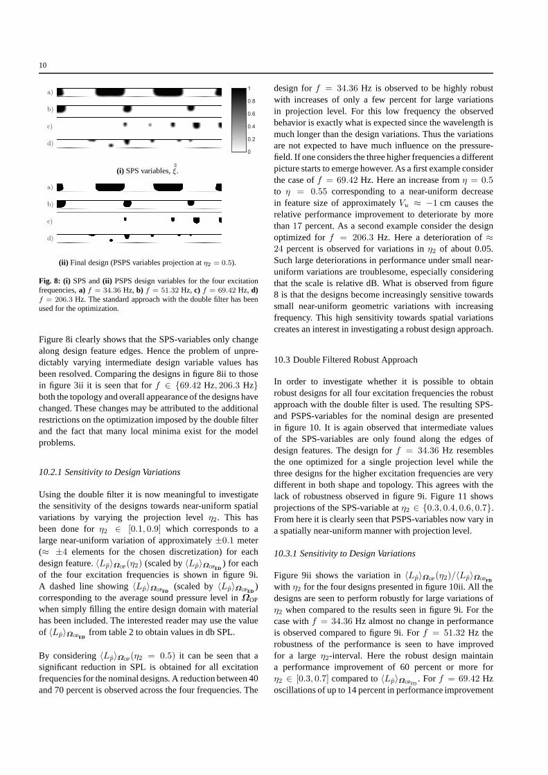
The double filter has been used with the standard approachreplacing the single filter. Results for the four excitationfrequencies are presented here. The SPS variables and finaldesigns (PSPS variables, projected atη2 = 0.5) are shownin figures 8i and 8ii, respectively.

2 The interested reader may find a derivation of the new sensitivitiesin appendix 14.1.

10

a)

b)

c)

d)

0

0.2

0.4

0.6

0.8

1

(i) SPS variables,˜ξ.

a)

b)

c)

d)

(ii) Final design (PSPS variables projection atη2 = 0.5).

Fig. 8: (i) SPS and(ii) PSPS design variables for the four excitationfrequencies,a) f = 34.36 Hz, b) f = 51.32 Hz, c) f = 69.42 Hz, d)f = 206.3 Hz. The standard approach with the double filter has beenused for the optimization.

Figure 8i clearly shows that the SPS-variables only changealong design feature edges. Hence the problem of unpre-dictably varying intermediate design variable values hasbeen resolved. Comparing the designs in figure 8ii to thosein figure 3ii it is seen that forf ∈ 69.42 Hz, 206.3 Hzboth the topology and overall appearance of the designs havechanged. These changes may be attributed to the additionalrestrictions on the optimization imposed by the double filterand the fact that many local minima exist for the modelproblems.

10.2.1 Sensitivity to Design Variations

Using the double filter it is now meaningful to investigatethe sensitivity of the designs towards near-uniform spatialvariations by varying the projection levelη2. This hasbeen done forη2 ∈ [0.1, 0.9] which corresponds to alarge near-uniform variation of approximately±0.1 meter(≈ ±4 elements for the chosen discretization) for eachdesign feature.〈Lp〉ΩOP(η2) (scaled by〈Lp〉ΩOPED

) for eachof the four excitation frequencies is shown in figure 9i.A dashed line showing〈Lp〉ΩOPFD

(scaled by〈Lp〉ΩOPED)

corresponding to the average sound pressure level inΩOP

when simply filling the entire design domain with materialhas been included. The interested reader may use the valueof 〈Lp〉ΩOPED

from table 2 to obtain values in db SPL.

By considering〈Lp〉ΩOP(η2 = 0.5) it can be seen that asignificant reduction in SPL is obtained for all excitationfrequencies for the nominal designs. A reduction between 40and 70 percent is observed across the four frequencies. The

design forf = 34.36 Hz is observed to be highly robustwith increases of only a few percent for large variationsin projection level. For this low frequency the observedbehavior is exactly what is expected since the wavelength ismuch longer than the design variations. Thus the variationsare not expected to have much influence on the pressure-field. If one considers the three higher frequencies a differentpicture starts to emerge however. As a first example considerthe case off = 69.42 Hz. Here an increase fromη = 0.5to η = 0.55 corresponding to a near-uniform decreasein feature size of approximatelyVu ≈ −1 cm causes therelative performance improvement to deteriorate by morethan17 percent. As a second example consider the designoptimized forf = 206.3 Hz. Here a deterioration of≈24 percent is observed for variations inη2 of about 0.05.Such large deteriorations in performance under small near-uniform variations are troublesome, especially consideringthat the scale is relative dB. What is observed from figure8 is that the designs become increasingly sensitive towardssmall near-uniform geometric variations with increasingfrequency. This high sensitivity towards spatial variationscreates an interest in investigating a robust design approach.

10.3 Double Filtered Robust Approach

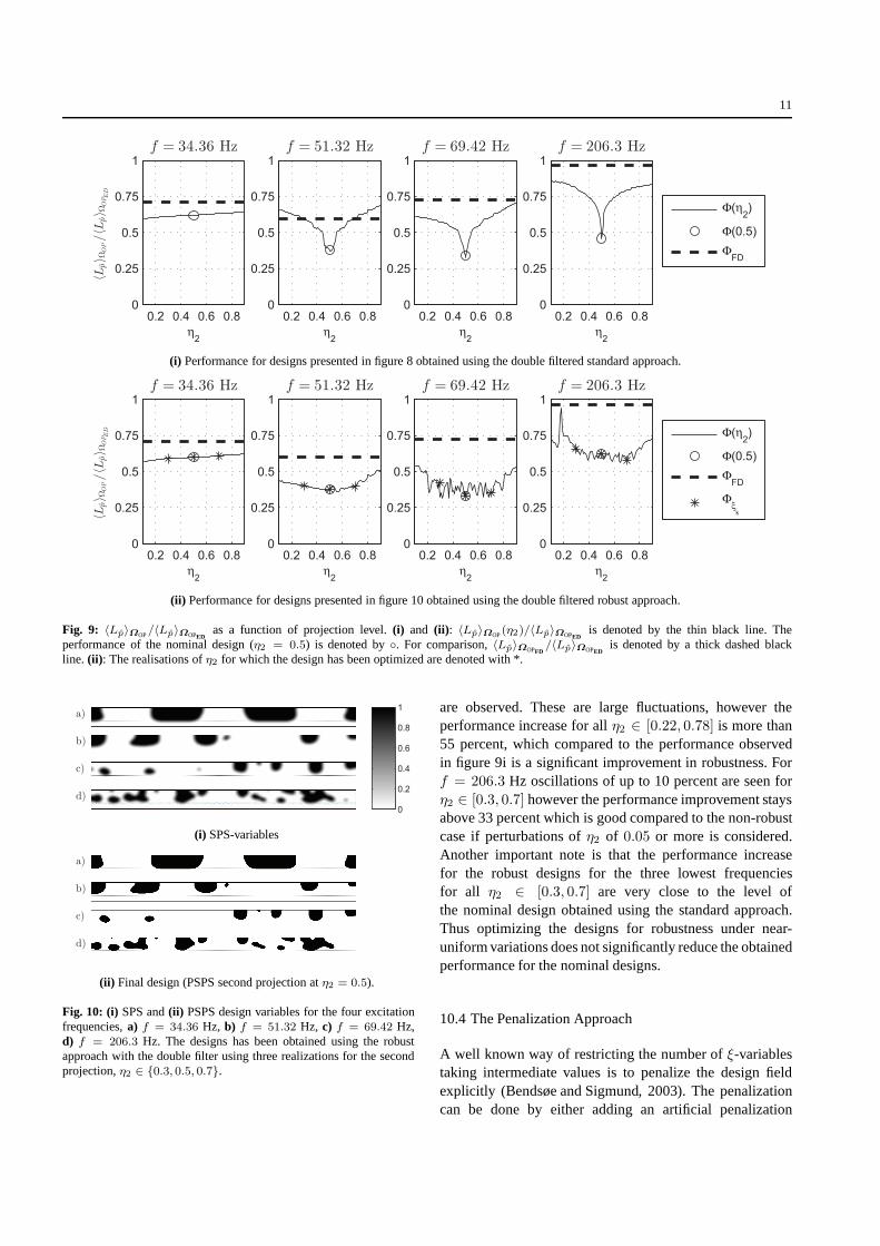
In order to investigate whether it is possible to obtainrobust designs for all four excitation frequencies the robustapproach with the double filter is used. The resulting SPS-and PSPS-variables for the nominal design are presentedin figure 10. It is again observed that intermediate valuesof the SPS-variables are only found along the edges ofdesign features. The design forf = 34.36 Hz resemblesthe one optimized for a single projection level while thethree designs for the higher excitation frequencies are verydifferent in both shape and topology. This agrees with thelack of robustness observed in figure 9i. Figure 11 showsprojections of the SPS-variable atη2 ∈ 0.3, 0.4, 0.6, 0.7.From here it is clearly seen that PSPS-variables now vary ina spatially near-uniform manner with projection level.

10.3.1 Sensitivity to Design Variations

Figure 9ii shows the variation in〈Lp〉ΩOP(η2)/〈Lp〉ΩOPFD

with η2 for the four designs presented in figure 10ii. All thedesigns are seen to perform robustly for large variations ofη2 when compared to the results seen in figure 9i. For thecase withf = 34.36 Hz almost no change in performanceis observed compared to figure 9i. Forf = 51.32 Hz therobustness of the performance is seen to have improvedfor a largeη2-interval. Here the robust design maintaina performance improvement of 60 percent or more forη2 ∈ [0.3, 0.7] compared to〈Lp〉ΩOPFD

. For f = 69.42 Hzoscillations of up to 14 percent in performance improvement

11

0.2 0.4 0.6 0.80

0.25

0.5

0.75

1f = 34.36 Hz

η2

〈Lp〉 Ω

OP/〈L

p〉 Ω

OPED

0.2 0.4 0.6 0.80

0.25

0.5

0.75

1f = 51.32 Hz

η2

0.2 0.4 0.6 0.80

0.25

0.5

0.75

1f = 69.42 Hz

η2

0.2 0.4 0.6 0.80

0.25

0.5

0.75

1f = 206.3 Hz

η2

Φ(η2)

Φ(0.5)

ΦFD

(i) Performance for designs presented in figure 8 obtained usingthe double filtered standard approach.

0.2 0.4 0.6 0.80

0.25

0.5

0.75

1f = 34.36 Hz

η2

〈Lp〉 Ω

OP/〈L

p〉 Ω

OPED

0.2 0.4 0.6 0.80

0.25

0.5

0.75

1f = 51.32 Hz

η2

0.2 0.4 0.6 0.80

0.25

0.5

0.75

1f = 69.42 Hz

η2

0.2 0.4 0.6 0.80

0.25

0.5

0.75

1f = 206.3 Hz

η2

Φ(η2)

Φ(0.5)

ΦFD

Φξ

k

(ii) Performance for designs presented in figure 10 obtained using the double filtered robust approach.

Fig. 9: 〈Lp〉ΩOP/〈Lp〉ΩOPEDas a function of projection level.(i) and (ii): 〈Lp〉ΩOP(η2)/〈Lp〉ΩOPED

is denoted by the thin black line. Theperformance of the nominal design (η2 = 0.5) is denoted by. For comparison,〈Lp〉ΩOPFD

/〈Lp〉ΩOPEDis denoted by a thick dashed black

line. (ii): The realisations ofη2 for which the design has been optimized are denoted with *.

a)

b)

c)

d)

0

0.2

0.4

0.6

0.8

1

(i) SPS-variables

a)

b)

c)

d)

(ii) Final design (PSPS second projection atη2 = 0.5).

Fig. 10: (i) SPS and(ii) PSPS design variables for the four excitationfrequencies,a) f = 34.36 Hz, b) f = 51.32 Hz, c) f = 69.42 Hz,d) f = 206.3 Hz. The designs has been obtained using the robustapproach with the double filter using three realizations forthe secondprojection,η2 ∈ 0.3, 0.5, 0.7.

are observed. These are large fluctuations, however theperformance increase for allη2 ∈ [0.22, 0.78] is more than55 percent, which compared to the performance observedin figure 9i is a significant improvement in robustness. Forf = 206.3 Hz oscillations of up to 10 percent are seen forη2 ∈ [0.3, 0.7] however the performance improvement staysabove 33 percent which is good compared to the non-robustcase if perturbations ofη2 of 0.05 or more is considered.Another important note is that the performance increasefor the robust designs for the three lowest frequenciesfor all η2 ∈ [0.3, 0.7] are very close to the level ofthe nominal design obtained using the standard approach.Thus optimizing the designs for robustness under near-uniform variations does not significantly reduce the obtainedperformance for the nominal designs.

10.4 The Penalization Approach

A well known way of restricting the number ofξ-variablestaking intermediate values is to penalize the design fieldexplicitly (Bendsøe and Sigmund, 2003). The penalizationcan be done by either adding an artificial penalization

12

a)

b)

c)

d)

(i) Excitation frequency,f = 34.36 Hz.

a)

b)

c)

d)

(ii) Excitation frequency,f = 51.32 Hz.

a)

b)

c)

d)

(iii) Excitation frequency,f = 69.42 Hz.

a)

b)

c)

d)

(iv) Excitation frequency,f = 206.3 Hz.

Fig. 11: Projection of SPS design variables at four differentη2-values,a) η2 = 0.3, b) η2 = 0.4, c) η2 = 0.6, d) η2 = 0.7 for the fourdesigns shown in figure 10i.

term, Φp, to the objective or introducing an additionalconstraint. Here we consider penalizing the filtered designvariables,ξ, as suggested by Borrvall and Petersson (2001).The penalization term given in (30) is used.

Φp(x) = αΦp

∫

ξ(x)(1− ξ(x))dΩd

/∫

dΩd, αΦp> 0.

(30)

The sensitivities of (30) with respect toξ are trivial tocalculate. The value ofΦp(x) is zero in areas withξ = 0

or ξ = 1 while it assumes its maximum value forξ = 1

2.

For sufficiently high values ofαΦpthe approach forces the

smoothed design variables towards 0/1 which will ensurenarrow ranges of intermediate values for the smootheddesign variables. This leads to near-uniform variations inthe design along the edges of design features when the

a)

b)

c)

d)

0

0.2

0.4

0.6

0.8

1

(i) Smoothed design variables

a)

b)

c)

d)

(ii) Projected final design atη = 0.5.

Fig. 12: (i) Smoothed and(ii) projected design variables for the fourexcitation frequencies,a) f = 34.36 Hz, b) f = 51.32 Hz, c) f =69.42 Hz, d) f = 206.3 Hz, obtained with the robust approach withthree realizations and the penalisation term added toΦ usingαΦp

=

6 · 10−3.

a)

b)

c)

d)

Fig. 13: Smoothed design variables presented in figure 12i for thefrequency,f = 206.3 Hz projected at,a) η = 0.3, b) η = 0.4,c) η = 0.6, d) η = 0.7.

projection level is varied. While this attribute is appealingone significant problem exists: The choice ofαΦp

. If αΦp

is chosen too large the penalization term will dominate theoptimization which will result in poorly performing designs.If αΦp

is chosen too small, however, the penalization willnot be effective and therefore the listed benefits are lost.

Designs obtained using the robust formulation where thepenalization term has been added to the objective usingαΦp

= 6 · 10−2 are presented here. This choice ofαΦp

illustrates both good and bad performance of the approachdistributed over the four excitation frequencies. A filterrange ofR = 20 has been used. The resulting designs arepresented in figure 12.

From the figure it is seen that at the three lower excitationfrequencies near 0/1ξ variables with smoothed edges alongdesign features are obtained. Meanwhile forf = 206.3 Hzthis property is seen to have disappeared. Figure 13 showsthe design obtained forf = 206.3 Hz projected at the four

13

different η-values. The design is seen to change topologyand vary non-uniformly. Hence the design has not beenoptimized for near-uniform spatial variations as intendeddue to a too weak penalization. Another worrying result isthe design obtained for the excitation frequencyf = 51.32Hz. Here the choice ofαΦp

= 6 · 10−2 turns out to betoo restrictive causing the optimization algorithm to getstuck in a local minimum with a poor performance. Theperformance obtained with this design is〈Lp〉ΩOP≈ 56 dBfor the nominal design which is more than 19 dB worse thanthe performance of the design obtained using the doublefilter approach, as may be deduced from figure 9ii combinedwith 〈Lp〉ΩOPED

from table 2.

These examples illustrate the main problem with thepenalization approach. That is, the correct choice ofαΦp

depends on the parameters of the problem in a non-obvious way which makes experimentation necessary foreach excitation frequency. On the other hand the examplesalso illustrate that ifαΦp is chosen correctly the approachmay work well. For the excitation frequencies studied hereresults similar to those obtained using the double filterapproach are obtained ifαΦp is chosen correctly.

11 Non-Uniform Design Variations

We have demonstrated that using the robust approachwith the double filter it is possible to create designswhich are highly robust towards near-uniform geometricvariations. In real applications however, during theproduction, installation and use of a given design it ismore likely that small non-uniform errors are introduced.An interesting question now becomes whether small non-uniform variations (NUVs) cause significant deteriorationsin performance for designs optimized for near-uniformvariations. A natural extension of this question is toinvestigate whether it is possible to create designs thatare more robust towards NUVs. In this section wedemonstrate that by using the robust approach withthe double filter it is possible to consider non-uniformvariations in the optimization. We present results showingthat the performance of designs optimized for near-uniformvariations may deteriorate significantly under small NUVs.Then we show that it is possible to obtain designs thatmaintain a more robust performance under both non-uniform and near-uniform variations by including samplesof the NUVs in the optimization process.

When taking NUVs into account during the optimizationprocess a high number of realizations is needed in order toassure that the space of possible perturbations is covered.In this case the computational resources required for thestandard FEM approach become a limiting factor. Therefore

a hybrid finite element and wave based method (FE-WBM)was implemented, in order to reduce the cost of modelingthe non-design domain, and used to obtain the resultspresented in the following. The wave based method wasproposed by Desmet (1998) and the hybrid FE-WBM byHal et al (2003). The hybrid FE-WBM has just recentlybeen applied to topology optimization by Goo et al (2014).The strength of the hybrid method is that it is possibleto significantly reduce the number of degrees of freedomused in the parts of the simulation domain where the modelparameters are homogeneous.

The hybrid method is applied by discretizing the non-design domainΩWBM = Ω\Ωd using a set of wave basisfunctions which are themselves solutions to the Helmholtzequation. This reduces the number of degrees of freedomneeded inΩWBM significantly. The design domainΩd isstill discretized exactly as described in section 5. Finally thetwo domains are coupled by introducing a set of couplingdegrees of freedom along the interface between theΩWBM

andΩd. SinceΩd is discretized as described in section 5 theparametrization ofξ(x), the formulation of the optimizationproblem, the application of the smoothing and projectionoperators and the interpretation of the design domain doesnot change in any way.

By applying the hybrid method to the present problemwhere the ratio of the full model domain to the designdomain is approximatelyΩd ≈ 0.1Ω the computationaltime was reduced by approximately a factor of ten. Weemphasize that other than a reduction in computational timethe application of the hybrid FE-WBM method does notchange the optimization problem in any way and as suchall results may be replicated using pure FEM if sufficientcomputational resources are available. The reportedperformance of all the designs obtained using the hybridmethod was acquired using a pure FEM discretization.

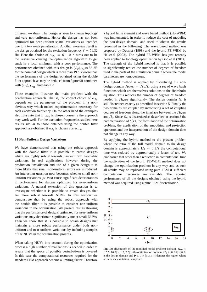
Fig. 14: Illustration of the modified model problem domain.ΩOP ∈[15.5, 16.5]×[1.5, 2.5] is the optimization domain,Ωd ∈ [0, 18]×[8, 9]is the design domain andP ∈ 0 × [1.3, 1.7] denotes the region wherean acoustic excitation is imposed.

14

a)

b)

c)

d)0.4

0.5

0.6

Fig. 15: Samples of the non-uniformly varying projection field fora)B = 2, C = 4

5π, b) B = 2, C = 6

5π, c) B = 4, C = 6

5π, d)

B = 8, C = 8

5π.

A slightly different model problem, illustrated in figure 14,was considered in the following. Here the vibrational sourcewas moved to one of the outer domain boundaries and wasimposed using (3) keepingU = 0.01, hence modeling avibrating piston set in the wall. The movement of the sourcewas done solely due to implementation choices made forthe WBM-FEM hybrid method which required placing thesource on the domain boundary.

It is possible to model NUVs in many ways. One way isto consider random non-uniform variations as was done forstructural and heat conduction problems by Schevenels et al(2011) and Lazarov et al (2012). In the present case weconsider only one type of non-random variation. Namelysinusoidal variations in one spatial direction and no variationin the other. This is only a small subset of all possible NUVsbut it works for illustrating the desired points. The NUVsare included in the optimization process by introducing avariable projection field,η(x), (Schevenels et al, 2011). Thisfield replaces the constant projection levelη, leading tovarying projection levels across the domain. When using thedouble filter approach it isη2 which is replaced with thevarying projection field. The NUVs in the projection levelhave been modeled as,

η2(x) = ηmin + (ηmax− ηmin) · P(A · cos(Bx+ C)). (31)

Here P is the normal cumulative distribution function withunit standard deviation and unit mean.ηmax ∈ ]ηmin, 1] andηmin ∈ [0, ηmax[ are the maximum and minimum projectionvalues, respectively.B andC were allowed to vary whileAwas kept fixed. Samples of the projection field for differentB andC are shown in figure 15.

For the results presented here the following values have beenused for the non-uniformly varying projection field:A = 6,B ∈ 2, 4, 8, C ∈ [0, 2π], ηmin = 0.4 andηmax = 0.6.The optimizations were initialized with the material fractionξini = 0.5 ∀ x ∈ Ωd and a filter radius ofR = 16 was used.

11.1 Imposing NUV on Robust Designs

In the following the two excitation frequencies,f ∈69.42, 206.3 Hz are considered. Optimized designs werecreated using the robust approach with the double filterand three realizations of the second projection atη2 ∈0.3, 0.5, 0.7. The designs are presented in figure 16.

a)

b)

Fig. 16: Nominal designs optimized using uniform variations for theexcitations frequenciesa) f = 69.42 Hz, andb) f = 206.3 Hz.

The designs were subjected to small non-uniform variationsgiven by (31). Figure 17 shows representative examplesof the non-uniform changes in the design optimized forf = 69.42 Hz when the variations are imposed. In the subfiguresb)-d) the white areas denote removed material whilethe black areas denote added material.

a)

b)

c)

d)

Fig. 17: Non-uniform variations in the design optimized forf = 69.42Hz. a) Design.b)-d) Difference between the nominal design and thenon-uniformly perturbed designs. White shows removed material andblack shows added material.

It is seen that the non-uniform variations are small (2.5-5 cm in terms of the model dimensions). Nevertheless asignificant reduction in performance is observed. Figure18 shows 〈Lp〉ΩOP(η2)/〈Lp〉ΩOPED

for varying projec-tion level, η ∈ [0.3, 0.7] overlaid with a graph of〈Lp〉ΩOP(η2,k(x))/〈Lp〉ΩOPED

for 80 different realizations ofthe non-uniform variations withA = 6, B ∈ 2, 4, 8, 16andC uniformly distributed at 20 points in[0, 2π[.

15

0.3 0.35 0.4 0.45 0.5 0.55 0.6 0.65 0.7

0.35

0.4

0.45

0.5

f = 69.42 Hz

η2

〈Lp〉 Ω

OP/〈Lp〉 Ω

OPED

0.3 0.35 0.4 0.45 0.5 0.55 0.6 0.65 0.7

0.6

0.65

0.7

f = 206.3 Hz

η2

〈Lp〉 Ω

OP/〈L

p〉 Ω

OPED

ΦUV

(η2) Φ

NUV(η

2,k(x)) Φ

ξk

Fig. 18: 〈Lp〉ΩOP/〈Lp〉ΩOPEDfor designs in figure 16 exposed to

near-uniform, ΦUV(η2), and non-uniform,ΦNUV(η2,k(x)), spatialvariations. The performance at the three realization for which thedesigns were optimized,Φξk

, are marked.

Figure 18 clearly shows the lack of robustness of the designstowards non-uniform variations. The observed performancedeteriorations are less significant than what was seen bycomparing designs optimized using the robust approach andusing the standard approach under near-uniform variations,however they are clearly still significant. Compared to thenominal designs (η2 = 0.5) a deterioration of up to 15% isseen for the design optimized atf = 69.42 Hz and up to9% for the design optimized atf = 206.3 Hz. Consideringcomparable near-uniform variations (η2 ∈ [0.4, 0.6]) weonly observe deteriorations of 5% and 1% respectively.

11.2 Optimizing for NUV

In order to reduce the observed deterioration in performanceunder non-uniform variations a new optimization wasperformed using the robust approach with the doublefilter. Here non-uniform variations were included in therealizations. A total of 18 realizations were used. Threeused the constant projection levelsη2 ∈ 0.3, 0.5, 0.7. Theremaining fifteen realizations used the variable projectionlevel given by (31) with all combinations ofB ∈ 2, 4, 8andC ∈ 2

5π, 4

5π, 6

5π, 8

5π, 2π. Figure 19 show the designs

resulting from the optimizations.

a)

b)

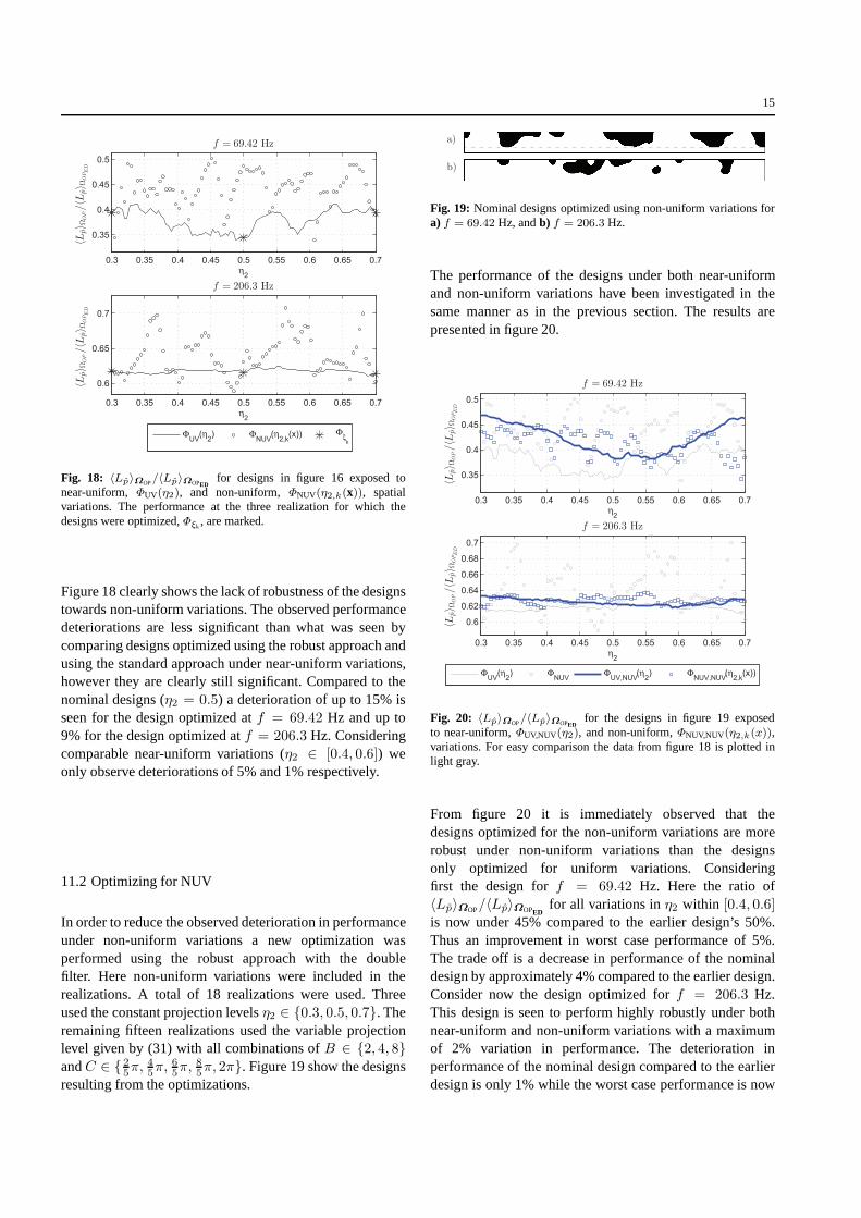
Fig. 19: Nominal designs optimized using non-uniform variations fora) f = 69.42 Hz, andb) f = 206.3 Hz.

The performance of the designs under both near-uniformand non-uniform variations have been investigated in thesame manner as in the previous section. The results arepresented in figure 20.

0.3 0.35 0.4 0.45 0.5 0.55 0.6 0.65 0.7

0.35

0.4

0.45

0.5

f = 69.42 Hz

η2

〈Lp〉 Ω

OP/〈L

p〉 Ω

OPED

0.3 0.35 0.4 0.45 0.5 0.55 0.6 0.65 0.7

0.6

0.62

0.64

0.66

0.68

0.7

f = 206.3 Hz

η2

〈Lp〉 Ω

OP/〈Lp〉 Ω

OPED

ΦUV

(η2) Φ

NUVΦ

UV,NUV(η

2) Φ

NUV,NUV(η

2,k(x))

Fig. 20: 〈Lp〉ΩOP/〈Lp〉ΩOPEDfor the designs in figure 19 exposed

to near-uniform,ΦUV,NUV(η2), and non-uniform,ΦNUV,NUV(η2,k(x)),variations. For easy comparison the data from figure 18 is plotted inlight gray.

From figure 20 it is immediately observed that thedesigns optimized for the non-uniform variations are morerobust under non-uniform variations than the designsonly optimized for uniform variations. Consideringfirst the design forf = 69.42 Hz. Here the ratio of〈Lp〉ΩOP/〈Lp〉ΩOPED

for all variations inη2 within [0.4, 0.6]

is now under 45% compared to the earlier design’s 50%.Thus an improvement in worst case performance of 5%.The trade off is a decrease in performance of the nominaldesign by approximately 4% compared to the earlier design.Consider now the design optimized forf = 206.3 Hz.This design is seen to perform highly robustly under bothnear-uniform and non-uniform variations with a maximumof 2% variation in performance. The deterioration inperformance of the nominal design compared to the earlierdesign is only 1% while the worst case performance is now

16

below 64% compared to the earlier 71%. Hence a 7% betterworst case performance.

A thorough study of the performance of the designs infigure 19 with more than 2500 realizations for uniformlydistributed value ofB ∈ [2, .., 16] and C ∈ [0, 2π]

was performed to assure the correctness of the conclusionsdrawn above. This test did not reveal any results thatcontradict our conclusions for the presented cases.

12 Varying the Filter Radius

This section investigates the behavior of the double filterapproach for varying filter radius. We consider the modelproblem in figure 14 and take the excitation frequencyto be, f = 69.42 Hz. We optimize using the doublyfiltered robust approach for four different filter radiiR1 ∈10, 20, 40, 60 elements,R2 = 1

2R1 and near-uniform

variations. We use six realizations for the projection level,η2,k ∈ 0.3, 0.38, 0.46, 0.54, 0.62, 0.7. The remainingparameters are set at the values given in table 1. The reasonfor using six realizations forη2,k instead of three as in theearlier cases is that it we found that forR1 ∈ 40, 60three realization for the second projection level are notenough to obtain a high performance across all values ofη2 ∈ [0.3, 0.7]. This finding is sensible since increasingR1

while keeping the variation inη2 fixed leads to an increasedspatial variation in the design. Figure 21 presents the finalSPS- and SPSP-variables for the four different cases.

a)

b)

c)

d)

0

0.2

0.4

0.6

0.8

1

(i) Final SPS-variables for four different filter radii .

a)

b)

c)

d)

(ii) Final SPSP-variables for four different filter radii projected atη2 = 0.5.

Fig. 21: (i) SPS and(ii) PSPS design variables obtained using therobust approach with different filter radii and six realizations of theuniform projection level atη2,k ∈ 0.3, 0.38, 0.46, 0.54, 0.62, 0.7 forthe excitation frequencyf = 69.42 Hz, discretized using(nx, ny) =(720, 360) finite elements. SPS-variables(i).a)R1 = 10 (i).b) R1 =20 (i).c) R1 = 40 (i).d) R1 = 60. (ii) PSPS-variables projected atη2 = 0.5 for designs in(i).

It is seen that the double filter performs as expected for allfilter radii, in the sense that it produces SPS-variables which

consists of areas of material (¯ξ(x) = 1) with smoothed

edges. Figure 22 shows the performance of each of the fourdesigns under near-uniform erosion/dilation performed byvarying η2 in the interval[0.1, 0.9]. It is observed that theperformance is similar in terms of the reduction in dB SPLfor all four cases inside the interval of optimization.

13 Conclusions

We considered the minimization of sound pressure in partof a 2D domain for an acoustic cavity problem by placingmaterial in another part of the domain using topologyoptimization. We showed that the direct application ofa standard technique for robust topology optimizationencounters a problem of uncontrollable intermediate designvariables making it unusable. A novel double filter wasintroduced and it was shown to alleviate the problem thusallowing for the application of the robust optimizationapproach. It was demonstrated that small near-uniformgeometric variations can cause significant deteriorationsinthe performance of designs optimized using the standardapproach. Applying the robust approach with the doublefilter and optimizing for near-uniform geometric variationswas shown to create highly robust designs under largenear-uniform variations for all investigated frequencies. Itwas then demonstrated that imposing small non-uniformvariations on designs optimized for near-uniform variationscould lead to smaller but still significant deteriorationsin performance. Finally it was shown to be possible toobtain designs which performed robustly under both near-uniform and selected non-uniform geometric variations bytaking both types of variations into account during theoptimization process. The proposed double filter approachis useful for highly shape sensitive optimization problemsas demonstrated here. For less sensitive problems standardsingle filter approaches may be sufficient. When solving theacoustic cavity problem considered in this paper for a widerfrequency band instead of for a single frequency (or narrowfrequency band) the extreme sensitivity disappears and theproblem may be solved using the single filter approach, seeappendix 14.2.

Acknowledgements This work was financially supported by VillumFonden through the research projectTopology Optimization - the NextGeneration NextTop.

17

0.2 0.4 0.6 0.80

0.25

0.5

0.75

1R1 = 0.25 m

η2

〈Lp〉 Ω

OP/〈L

p〉 Ω

OPED

0.2 0.4 0.6 0.80

0.25

0.5

0.75

1R1 = 0.50 m

η2

0.2 0.4 0.6 0.80

0.25

0.5

0.75

1R1 = 1 m

η2

0.2 0.4 0.6 0.80

0.25

0.5

0.75

1R1 = 1.5 m

η2

Φ(η2)

Φ(0.5)

ΦFD

Φξ

k

Fig. 22: 〈Lp〉ΩOP/〈Lp〉ΩOPEDas a function of projection level for designs presented in figure 21, obtained using the double filtered robust approach,

under uniform erosion/dilation.〈Lp〉ΩOP(η2)/〈Lp〉ΩOPEDis denoted by the thin black line. The performance of the nominal design (η2 = 0.5) is

denoted by. For comparison,〈Lp〉ΩOPFD/〈Lp〉ΩOPED

is denoted by a thick dashed black line. The realizations ofη2 for which the design has beenoptimized are denoted with *.

14 Appendix

14.1 Derivation of Sensitivities for the Double Filter

The sensitivities,dΦdξi, for the double filter may be derived as

follows:

1. Apply the chain rule for calculating the sensitivities.

dΦdξi

=∑

j,k,l,h

∂ξl∂ξi

∂¯ξh

∂ξl

∂˜ξk

∂¯ξh

∂¯ξj

∂˜ξk

dΦ

d¯ξj

. (32)

2. Eliminate two sums using the fact that∂¯ξh

∂ξl= 0 ∀ l 6= h

and that∂¯¯ξj

∂˜ξk

= 0 ∀ k 6= j due to the locality of (23).

dΦdξi

=∑

j

∑

h

∂ξh∂ξi

∂¯ξh

∂ξh

∂˜ξj

∂¯ξh

∂¯ξj

∂˜ξj

dΦ

d¯ξj

i ∈ 1, 2, ..., N.

(33)

3. Utilize that ξh only depends on the design variablesξi within the density filter radius reducing the sum

over h significantly. The same argument applied to˜ξj

and ¯ξh reduces the sum overj. The set of indices

for the dependent variables are denoted,Be,i andBe,h

respectively. The sensitivities now take the form,

dΦdξi

=∑

j∈Be,h

∑

h∈Be,i

∂ξh∂ξi

∂ ¯ξh

∂ξh

∂˜ξj

∂ ¯ξh

∂¯ξj

∂˜ξj

dΦ

d¯ξj

. (34)

4. Rewriting the expression gives,

dΦdξi

=∑

h∈Be,i

∂ξh∂ξi

∂ ¯ξh

∂ξh

∑

j∈Be,h

∂˜ξj

∂ ¯ξh

∂¯ξj

∂˜ξj

dΦ

d¯ξj

. (35)

5. For a givenh the expression in the bracket in (35) onlydepends onj. Thus we may define,

∆Φh =∑

j∈Be,h

∂˜ξj

∂ ¯ξh

∂¯ξj

∂˜ξj

dΦ

d¯ξj

, h ∈ 1, 2, ..., N. (36)

This illustrates that the application of the double filtersimply corresponds to applying the single filter twice.

14.2 Application of Robust Approach for Frequency Bands

Single frequency problems have been the focus of thepaper due to the high sensitivity in the performance ofthe optimized designs under geometric variations. In thissection we provide an example showing that it of courseis possible to apply the proposed method for a band offrequencies as well. However, as will be demonstrated,the case of minimizing the mean sound pressure across afrequency band is much less interesting in the context ofthis paper, since this quantity is far less sensitive towardsgeometric variations in the design. A requirement forconsidering optimization for a band of frequencies is thata small amount of damping is added to the model problemto avoid problems caused by resonances in the frequencyband of interest, which when undamped, leads to a nearsingular problem at the resonance and a sound pressuregoing towards infinity. The need for damping has nothingto do with the double filter or the robust approach andmust be added regardless of the optimization strategy. Massproportional damping is introduced by adding the term”αdamp i ωp” to equation (7) whereαdamp = 0.01 is thedamping factor.

In the following we consider the model problem presentedin figure 14 and seek to minimize the mean of the average

18

sound pressure inΩOP over a 1/3 octave frequency band,fb ≈ [61.85, 77.92] Hz, centered at,fc = 62.5 Hz. Theobjective function may thus be stated as,

Φ(ξ) =1

Ni

Ni∑

i=1

1

AOP

∫

|p(¯ξ, fi)|2dΩOP, (37)

wherefi are the frequencies optimized for andNi is thenumber of frequencies. An optimization is performed usingthe standard approach with the double filter and the secondprojection atη2 = 0.5. For comparison an optimization isperformed using the robust approach with double filteringand five realizations of the second projection level,η2 ∈0.3, 0.4, 0.5, 0.6, 0.7. For both cases we useNi = 20

and consider equidistant frequencies infb including bothendpoints. For the PDE problem we use a pure FEMdiscretization withNx = 216, Ny = 108 elements. Afilter range ofR1 = 5 elements is used. Figure 23 shows theresulting SPS and SPSP variables for the two optimizations.

a)

b)0.2

0.4

0.6

0.8

(i) Final SPS-variables for designs optimized for a frequency band.

a)

b)

(ii) Final SPSP-variables for designs optimized for a frequencyband.

Fig. 23: (i) SPS and(ii) PSPS design variables obtained using the a)standard and b) robust approach for the 1/3 octave frequencybandoptimization.

Figure 24 shows the mean of the average sound pressurelevel inΩOP over the 1/3 octave frequency band,〈Lp〉ΩOP,fb,scaled by the same quantity inΩOP for the empty cavity,〈Lp〉ΩOPED ,fb ≈ 89.79 dB, as a function of projectionlevel η2, for both the standard and the robust approach.The mean over the frequency is calculated using 100equidistant frequencies infb. This variation in projectionlevel corresponds to a near-uniform erosion/dilation of 1element or approximately 8 cm in the design. The presentedresults have been evaluated with the same amount ofdamping as the one used in the optimization.

0.3 0.35 0.4 0.45 0.5 0.55 0.6 0.65 0.70.7

0.75

0.8

0.85

0.9

0.95

1

η2

〈Lp〉 Ω

OP,fb/〈L

p〉 Ω

OPED,fb

ΦStandard

(η2) Φ

Robust(η

2)

Fig. 24: 〈Lp〉ΩOP,fb/〈Lp〉ΩOPED,fb

for the designs in figure 23 undernear-uniform variations imposed by varyingη2. The performance ofthe designs is seen to be almost constant under the prescribed uniformvariations.

From the figure it is clearly observed that both the standardand robust approach produce results which do not show anysignificant sensitivity towards uniform erosion or dilation ofthe design. It is noted that the robust approach producesa design with better performance. This is likely due tothe additional restrictions on the optimization when usingthe robust approach which eliminates the local minimumtrapping the optimization performed with the standardapproach.

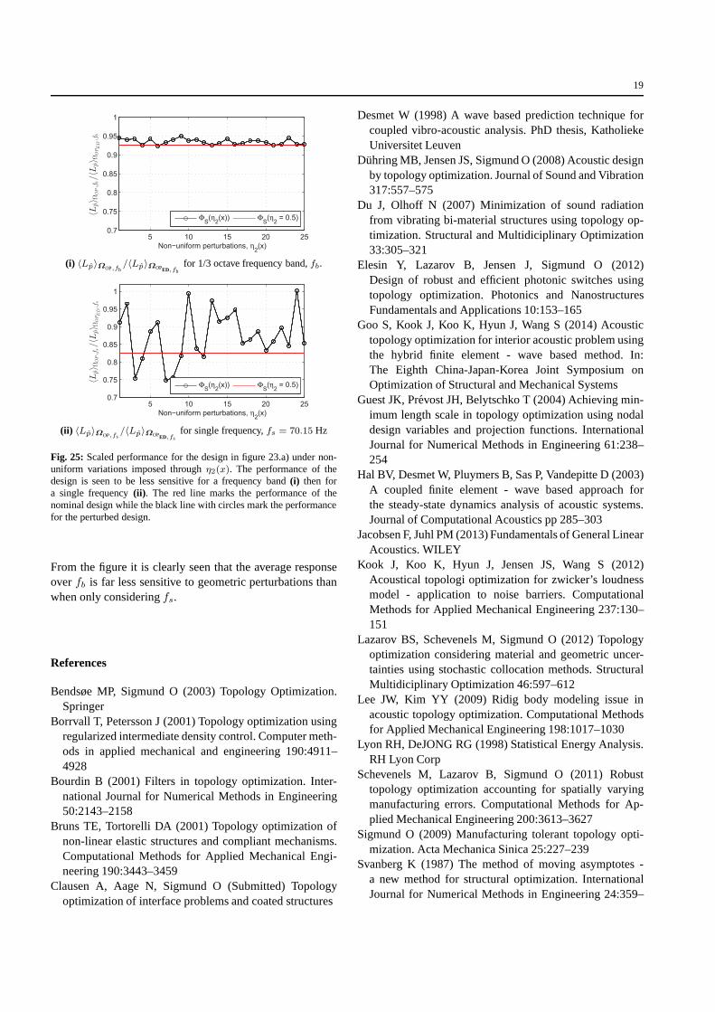
An investigation of the sensitivity of the performance undernon-uniform geometric variations for the design optimizedusing the standard approach is also performed. Here it isshown that, just as for the uniform geometric perturbations,the sensitivity drops significantly when considering a bandof frequencies compared to a single frequency. Twenty fivenon-uniform geometric variations are applied as describedin section 11 usingA = 6, B ∈ 2, 3.5, 5, 6.5, 8,C ∈ 2π · 1, 2, 3, 4, 5, ηmin = 0.3, ηmax = 0.7.Figure 25.(i) show the sensitivity of the performance underthe twenty five non-uniform geometric variations for theaverage response overfb while figure 25.(ii) show theperformance sensitivity under the same twenty five non-uniform geometric variations for the single frequencyfs =

70.15 Hz.

19

5 10 15 20 250.7

0.75

0.8

0.85

0.9

0.95

1

Non−uniform perturbations, η2(x)

〈Lp〉 Ω

OP,fb/〈L

p〉 Ω

OPED,fb

ΦS(η

2(x)) Φ

S(η

2 = 0.5)

(i) 〈Lp〉ΩOP,fb/〈Lp〉ΩOPED,fb

for 1/3 octave frequency band,fb.

5 10 15 20 250.7

0.75

0.8

0.85

0.9

0.95

1

Non−uniform perturbations, η2(x)

〈Lp〉 Ω

OP,fs/〈Lp〉 Ω

OPED,fs

ΦS(η

2(x)) Φ

S(η

2 = 0.5)

(ii) 〈Lp〉ΩOP,fs/〈Lp〉ΩOPED,fs

for single frequency,fs = 70.15 Hz

Fig. 25: Scaled performance for the design in figure 23.a) under non-uniform variations imposed throughη2(x). The performance of thedesign is seen to be less sensitive for a frequency band(i) then fora single frequency(ii). The red line marks the performance of thenominal design while the black line with circles mark the performancefor the perturbed design.

From the figure it is clearly seen that the average responseoverfb is far less sensitive to geometric perturbations thanwhen only consideringfs.

References

Bendsøe MP, Sigmund O (2003) Topology Optimization.Springer

Borrvall T, Petersson J (2001) Topology optimization usingregularized intermediate density control. Computer meth-ods in applied mechanical and engineering 190:4911–4928

Bourdin B (2001) Filters in topology optimization. Inter-national Journal for Numerical Methods in Engineering50:2143–2158

Bruns TE, Tortorelli DA (2001) Topology optimization ofnon-linear elastic structures and compliant mechanisms.Computational Methods for Applied Mechanical Engi-neering 190:3443–3459

Clausen A, Aage N, Sigmund O (Submitted) Topologyoptimization of interface problems and coated structures

Desmet W (1998) A wave based prediction technique forcoupled vibro-acoustic analysis. PhD thesis, KatholiekeUniversitet Leuven

Duhring MB, Jensen JS, Sigmund O (2008) Acoustic designby topology optimization. Journal of Sound and Vibration317:557–575

Du J, Olhoff N (2007) Minimization of sound radiationfrom vibrating bi-material structures using topology op-timization. Structural and Multidiciplinary Optimization33:305–321

Elesin Y, Lazarov B, Jensen J, Sigmund O (2012)Design of robust and efficient photonic switches usingtopology optimization. Photonics and NanostructuresFundamentals and Applications 10:153–165

Goo S, Kook J, Koo K, Hyun J, Wang S (2014) Acoustictopology optimization for interior acoustic problem usingthe hybrid finite element - wave based method. In:The Eighth China-Japan-Korea Joint Symposium onOptimization of Structural and Mechanical Systems

Guest JK, Prevost JH, Belytschko T (2004) Achieving min-imum length scale in topology optimization using nodaldesign variables and projection functions. InternationalJournal for Numerical Methods in Engineering 61:238–254

Hal BV, Desmet W, Pluymers B, Sas P, Vandepitte D (2003)A coupled finite element - wave based approach forthe steady-state dynamics analysis of acoustic systems.Journal of Computational Acoustics pp 285–303

Jacobsen F, Juhl PM (2013) Fundamentals of General LinearAcoustics. WILEY

Kook J, Koo K, Hyun J, Jensen JS, Wang S (2012)Acoustical topologi optimization for zwicker’s loudnessmodel - application to noise barriers. ComputationalMethods for Applied Mechanical Engineering 237:130–151

Lazarov BS, Schevenels M, Sigmund O (2012) Topologyoptimization considering material and geometric uncer-tainties using stochastic collocation methods. StructuralMultidiciplinary Optimization 46:597–612

Lee JW, Kim YY (2009) Ridig body modeling issue inacoustic topology optimization. Computational Methodsfor Applied Mechanical Engineering 198:1017–1030

Lyon RH, DeJONG RG (1998) Statistical Energy Analysis.RH Lyon Corp

Schevenels M, Lazarov B, Sigmund O (2011) Robusttopology optimization accounting for spatially varyingmanufacturing errors. Computational Methods for Ap-plied Mechanical Engineering 200:3613–3627

Sigmund O (2009) Manufacturing tolerant topology opti-mization. Acta Mechanica Sinica 25:227–239

Svanberg K (1987) The method of moving asymptotes -a new method for structural optimization. InternationalJournal for Numerical Methods in Engineering 24:359–

20

373Wadbro E (2014) Analysis and design of acoustic transition

sections for impedance matching and mode conversion.Structural and Multidiciplinary Optimization 50:395–408

Wadbro E, Berggren M (2006) Topology optimization ofan acoustic horn. Computational Methods for AppliedMechanical Engineering 196:420–436

Wang F, Jensen JS, Sigmund O (2011a) Robust topologyoptimization of photonic crystal waveguides with tai-lored dispersion properties. Optical Society of America28:387–397

Wang F, Lazarov BS, Sigmund O (2011b) On pro-jection methods, convergence and robust formulationsin topology optimization. Structural MultidiciplinaryOptimization 43:767–784

Xu S, Cai Y, Cheng G (2010) Volume preserving nonlineardensity filter based on heaviside projections. Structuraland Multidiciplinary Optimization 41:495–505

Yoon GH, Jensen JS, Sigmund O (2007) Topologyoptimization of acoustic-structure interaction problemsusing a mixed finite element formulation. InternationalJournal for Numerical Methods in Engineering 70:1049–1075