CPSC 340:Machine Learning and Data Mining

Feature Engineering

Fall 2019

Admin

• Assignment 3: grades posted soon.

• Assignment 4: due Friday of next week.

• Midterm: grades soon.

– Can view exams during my office hours next week or the week after.

• Projects: may get contacted by TA if there are concerns.

• We got a complaint about people entering classroom too early.

– Please wait until 1:50pm before entering classroom.

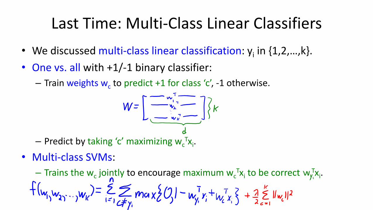
Last Time: Multi-Class Linear Classifiers

• We discussed multi-class linear classification: yi in {1,2,…,k}.

• One vs. all with +1/-1 binary classifier:

– Train weights wc to predict +1 for class ‘c’, -1 otherwise.

– Predict by taking ‘c’ maximizing wcTxi.

• Multi-class SVMs:

– Trains the wc jointly to encourage maximum wcTxi to be correct Txi.

Multi-Class Logistic Regression

• We derived binary logistic loss by smoothing a degenerate ‘max’.– A degenerate constraint in the multi-class case can be written as:

• We want the right side to be as small as possible.

• Let’s smooth the max with the log-sum-exp:

– This is no longer degenerate: with W=0 this gives a loss of log(k).

• Called the softmax loss, the loss for multi-class logistic regression.

Multi-Class Logistic Regression

• We sum the loss over examples and add regularization:

• This objective is convex (should be clear for 1st and 3rd terms).– It’s differentiable so you can use gradient descent.

• When k=2, equivalent to using binary logistic loss.– Not obvious at the moment.

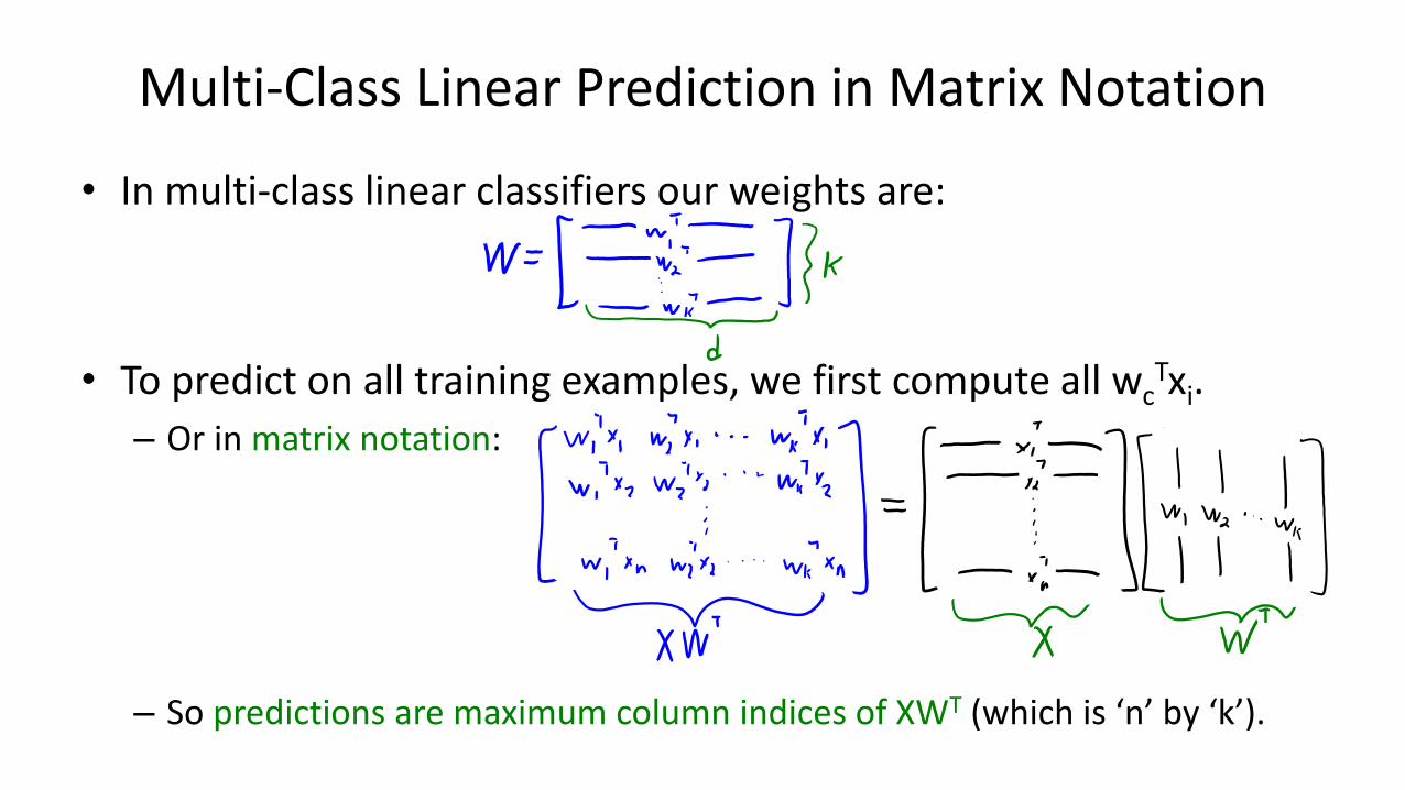
Multi-Class Linear Prediction in Matrix Notation

• In multi-class linear classifiers our weights are:

• To predict on all training examples, we first compute all wcTxi.

– Or in matrix notation:

– So predictions are maximum column indices of XWT (which is ‘n’ by ‘k’).

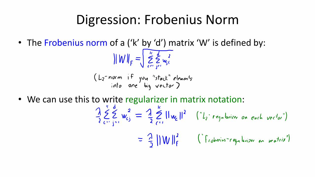
Digression: Frobenius Norm

• The Frobenius norm of a (‘k’ by ‘d’) matrix ‘W’ is defined by:

• We can use this to write regularizer in matrix notation:

(pause)

Feature Engineering

• “…some machine learning projects succeed and some fail. What makes the difference? Easily the most important factor is the features used.”

– Pedro Domingos

• “Coming up with features is difficult, time-consuming, requires expert knowledge. "Applied machine learning" is basically feature engineering.”

– Andrew Ng

Feature Engineering

• Better features usually help more than a better model.

• Good features would ideally:

– Allow learning with few examples, be hard to overfit with many examples.

– Capture most important aspects of problem.

– Reflects invariances (generalize to new scenarios).

• There is a trade-off between simple and expressive features:

– With simple features overfitting risk is low, but accuracy might be low.

– With complicated features accuracy can be high, but so is overfitting risk.

Feature Engineering

• The best features may be dependent on the model you use.

• For counting-based methods like naïve Bayes and decision trees:

– Need to address coupon collecting, but separate relevant “groups”.

• For distance-based methods like KNN:

– Want different class labels to be “far”.

• For regression-based methods like linear regression:

– Want labels to have a linear dependency on features.

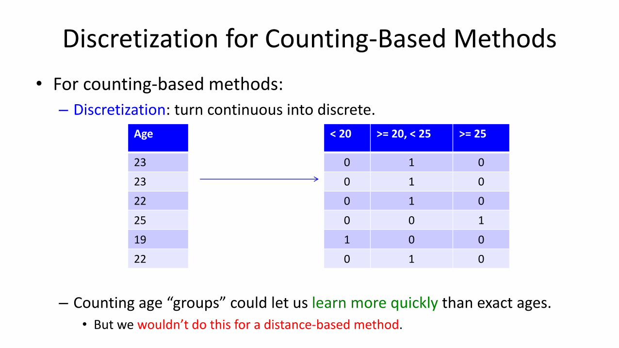
Discretization for Counting-Based Methods

• For counting-based methods:

– Discretization: turn continuous into discrete.

– Counting age “groups” could let us learn more quickly than exact ages.

• But we wouldn’t do this for a distance-based method.

Age

23

23

22

25

19

22

< 20 >= 20, < 25 >= 25

0 1 0

0 1 0

0 1 0

0 0 1

1 0 0

0 1 0

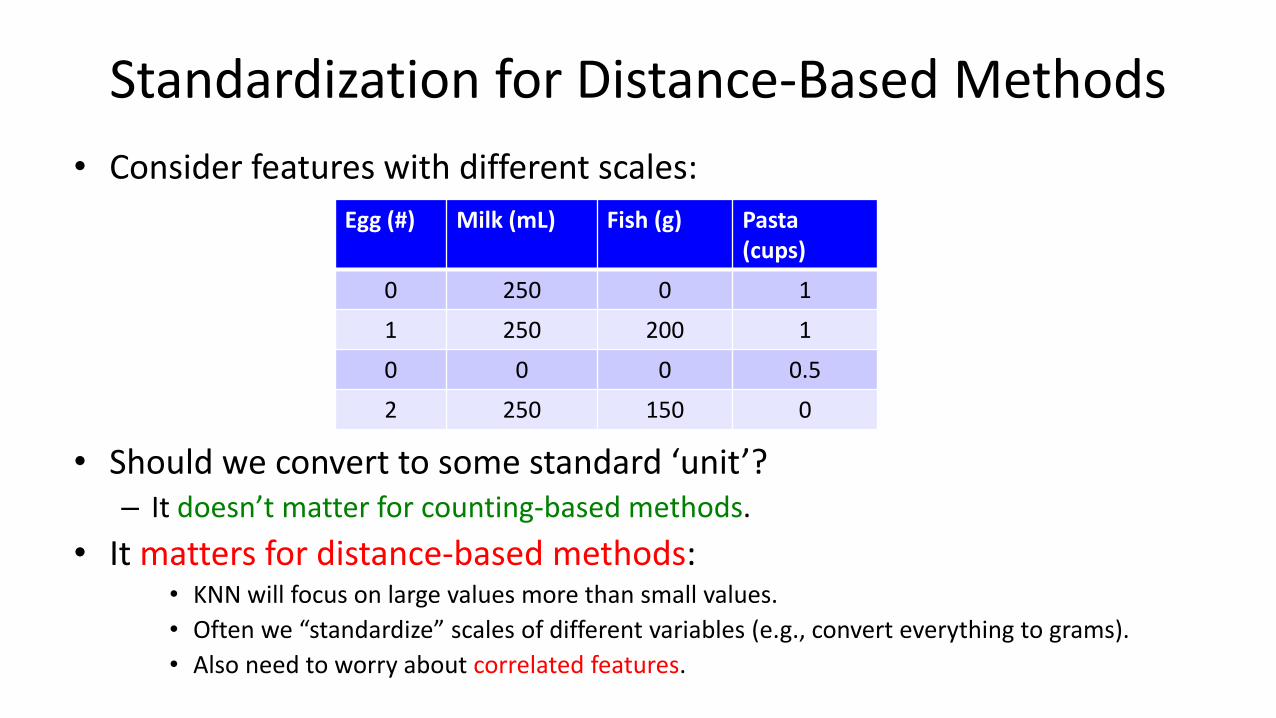
Standardization for Distance-Based Methods

• Consider features with different scales:

• Should we convert to some standard ‘unit’?– It doesn’t matter for counting-based methods.

• It matters for distance-based methods:• KNN will focus on large values more than small values.

• Often we “standardize” scales of different variables (e.g., convert everything to grams).

• Also need to worry about correlated features.

Egg (#) Milk (mL) Fish (g) Pasta(cups)

0 250 0 1

1 250 200 1

0 0 0 0.5

2 250 150 0

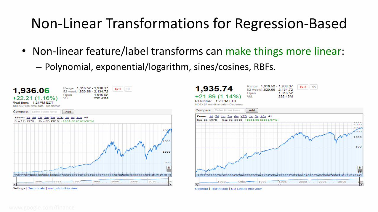
Non-Linear Transformations for Regression-Based

• Non-linear feature/label transforms can make things more linear:

– Polynomial, exponential/logarithm, sines/cosines, RBFs.

www.google.com/finance

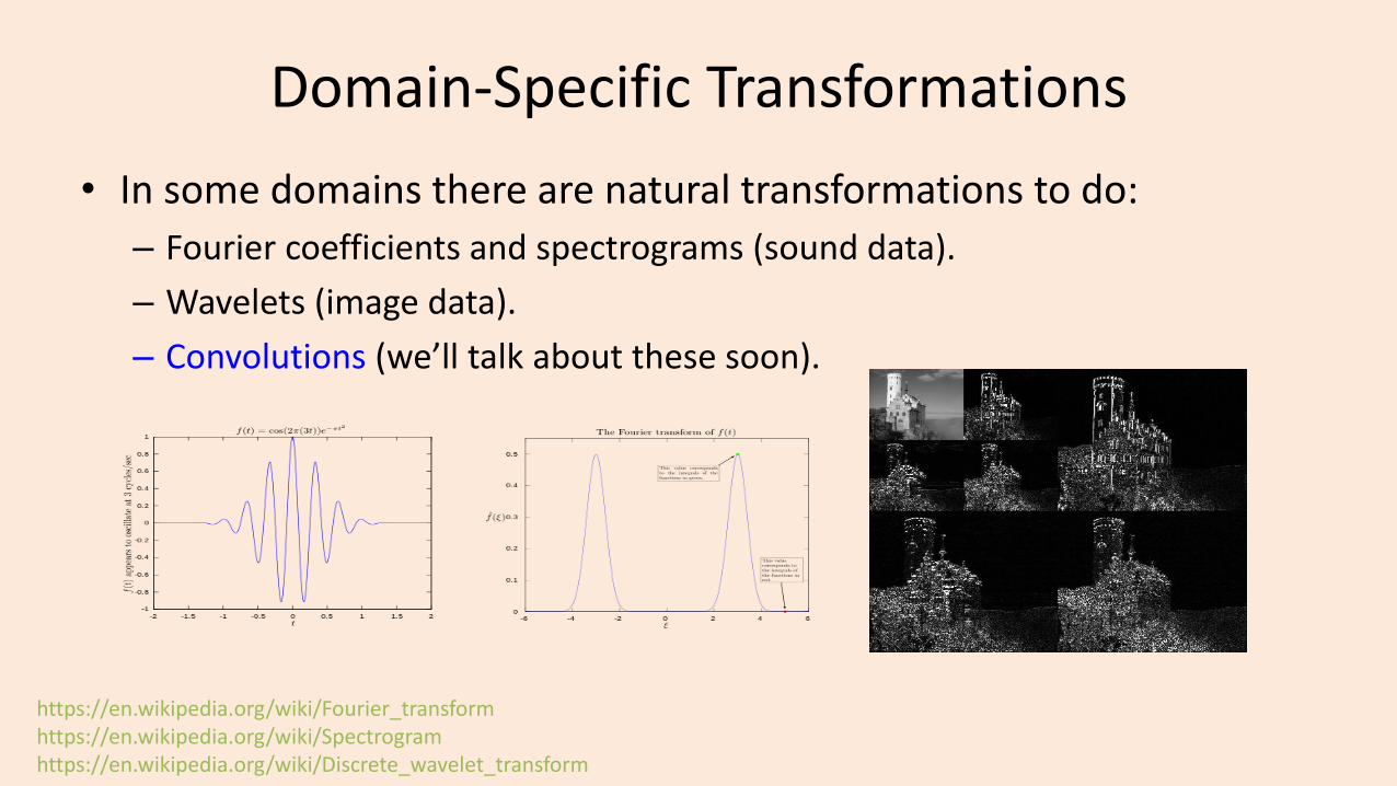
Domain-Specific Transformations

• In some domains there are natural transformations to do:

– Fourier coefficients and spectrograms (sound data).

– Wavelets (image data).

– Convolutions (we’ll talk about these soon).

https://en.wikipedia.org/wiki/Fourier_transformhttps://en.wikipedia.org/wiki/Spectrogramhttps://en.wikipedia.org/wiki/Discrete_wavelet_transform

Discussion of Feature Engineering

• The best feature transformations are application-dependent.

– It’s hard to give general advice.

• My advice: ask the domain experts.

– Often have idea of right discretization/standardization/transformation.

• If no domain expert, cross-validation will help.

– Or if you have lots of data, use deep learning methods from Part 5.

• Next: I’ll give some features used for text/image applications.

(pause)

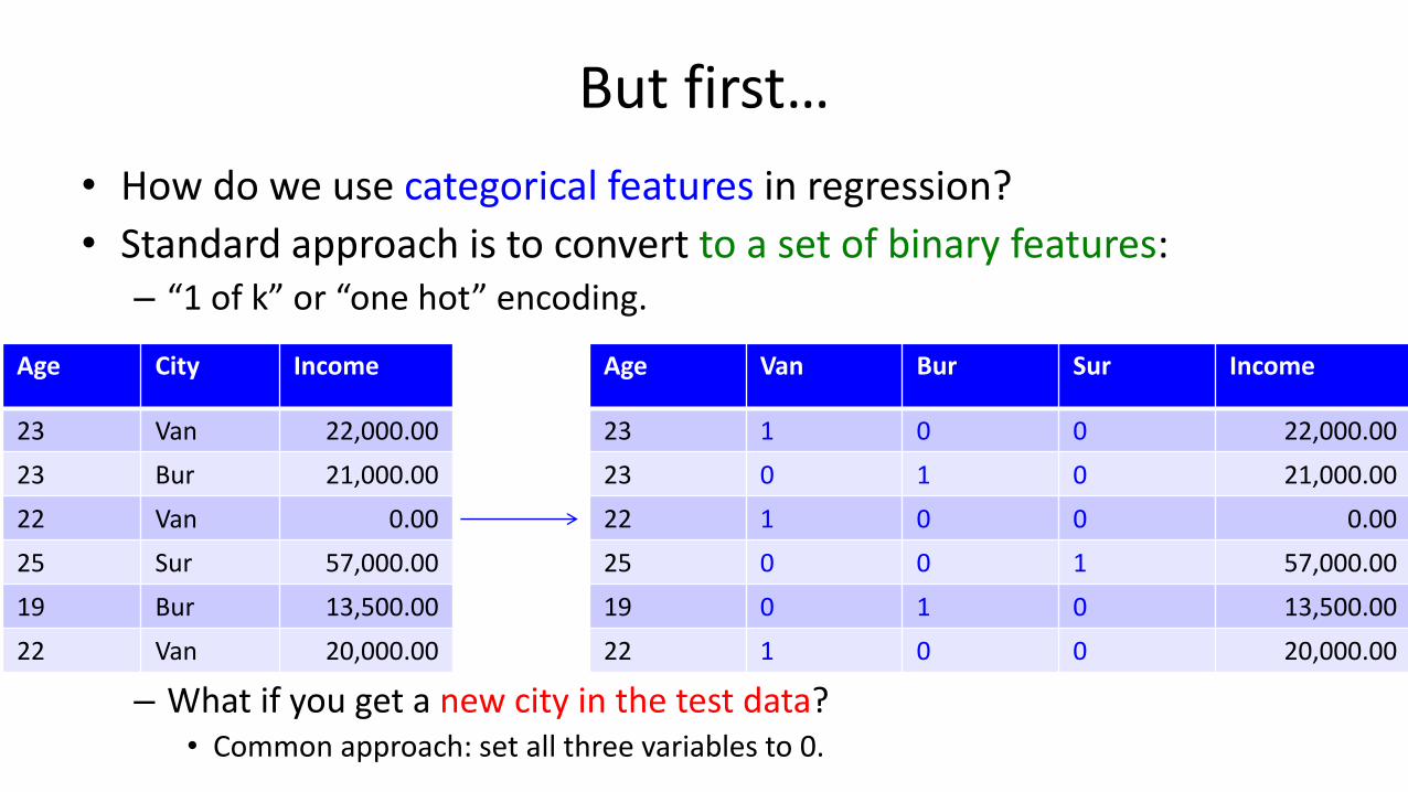
But first…

• How do we use categorical features in regression?

• Standard approach is to convert to a set of binary features:– “1 of k” or “one hot” encoding.

– What if you get a new city in the test data?• Common approach: set all three variables to 0.

Age City Income

23 Van 22,000.00

23 Bur 21,000.00

22 Van 0.00

25 Sur 57,000.00

19 Bur 13,500.00

22 Van 20,000.00

Age Van Bur Sur Income

23 1 0 0 22,000.00

23 0 1 0 21,000.00

22 1 0 0 0.00

25 0 0 1 57,000.00

19 0 1 0 13,500.00

22 1 0 0 20,000.00

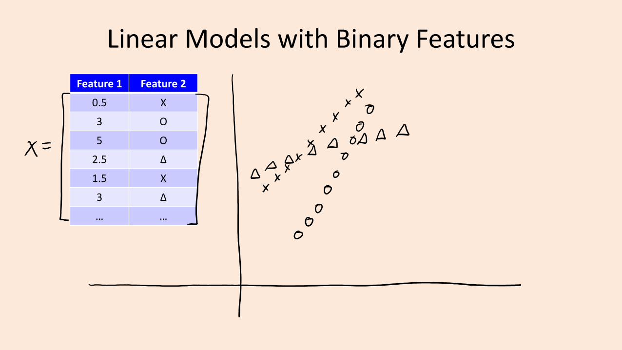
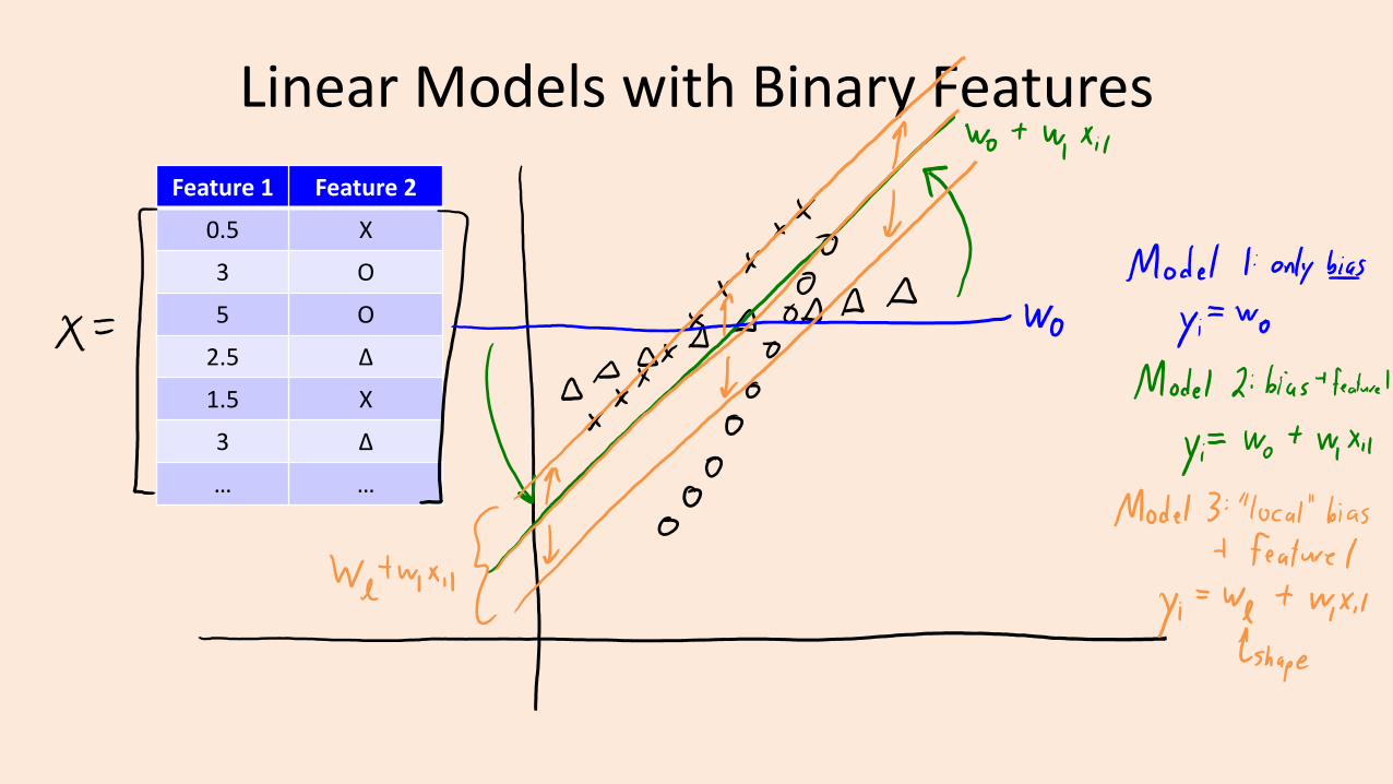
Digression: Linear Models with Binary Features

• What is the effect of a binary features on linear regression?

• Suppose we use a bag of words:– With 3 words {“hello”, “Vicodin”, “340“} our model would be:

– If e-mail only has “hello” and “340” our prediction is:

• So having the binary feature ‘j’ increases ො𝑦i by the fixed amount wj.– Predictions are a bit like naïve Bayes where we combine features independently.

– But now we’re learning all wj together so this tends to work better.

Text Example 1: Language Identification

• Consider data that doesn’t look like this:

• But instead looks like this:

• How should we represent sentences using features?

A (Bad) Universal Representation

• Treat character in position ‘j’ of the sentence as a categorical feature.• “fais ce que tu veux” => xi = [f a i s ‘’ c e ‘’ q u e ‘’ t u ‘’ v e u x .]

• “Pad” end of the sentence up to maximum #characters:• “fais ce que tu veux” => xi = [f a i s ‘’ c e ‘’ q u e ‘’ t u ‘’ v e u x . γ γ γ γ γ γ γ γ …]

• Advantage: – No information is lost, KNN can eventually solve the problem.

• Disadvantage: throws out everything we know about language.– Needs to learn that “veux” starting from any position indicates “French”.

• Doesn’t even use that sentences are made of words (this must be learned).

– High overfitting risk, you will need a lot of examples for this easy task.

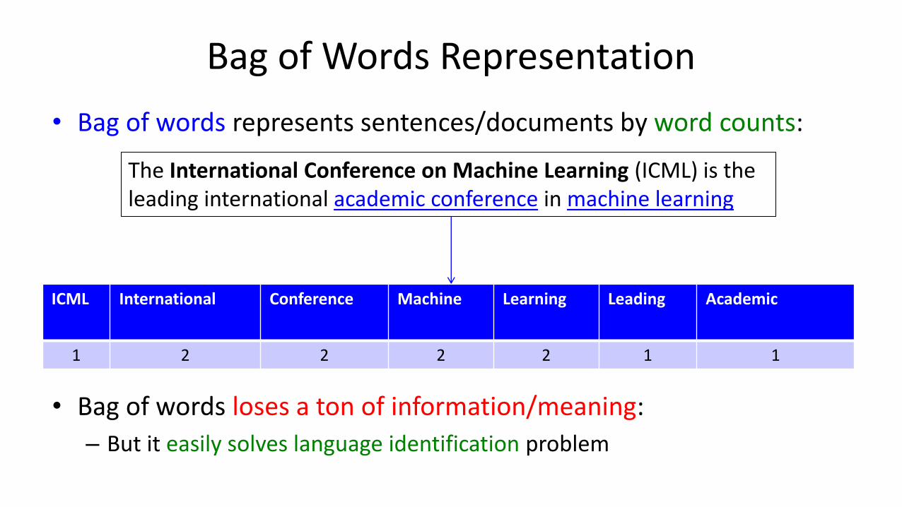
Bag of Words Representation

• Bag of words represents sentences/documents by word counts:

• Bag of words loses a ton of information/meaning:

– But it easily solves language identification problem

The International Conference on Machine Learning (ICML) is the leading international academic conference in machine learning

ICML International Conference Machine Learning Leading Academic

1 2 2 2 2 1 1

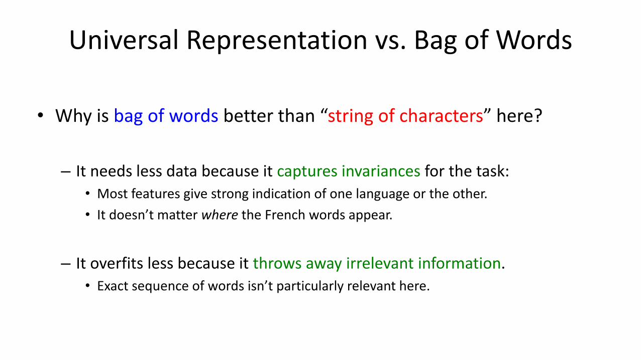
Universal Representation vs. Bag of Words

• Why is bag of words better than “string of characters” here?

– It needs less data because it captures invariances for the task:

• Most features give strong indication of one language or the other.

• It doesn’t matter where the French words appear.

– It overfits less because it throws away irrelevant information.

• Exact sequence of words isn’t particularly relevant here.

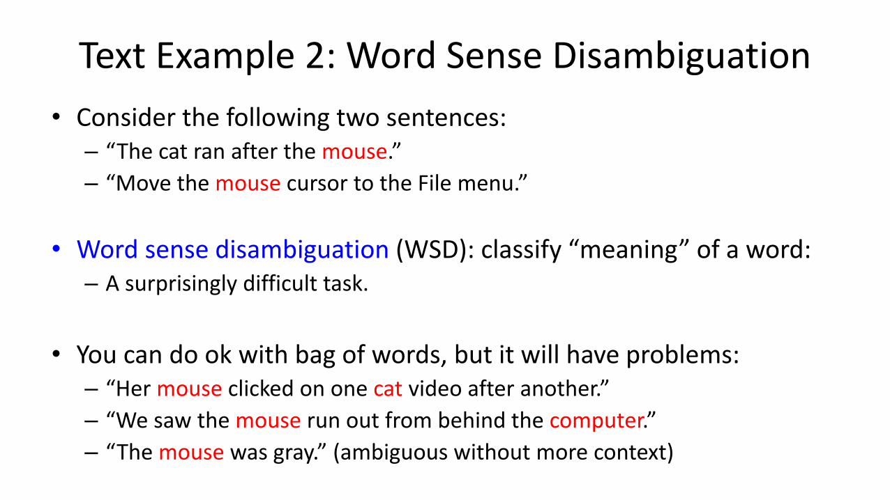
Text Example 2: Word Sense Disambiguation

• Consider the following two sentences:– “The cat ran after the mouse.”

– “Move the mouse cursor to the File menu.”

• Word sense disambiguation (WSD): classify “meaning” of a word:– A surprisingly difficult task.

• You can do ok with bag of words, but it will have problems:– “Her mouse clicked on one cat video after another.”

– “We saw the mouse run out from behind the computer.”

– “The mouse was gray.” (ambiguous without more context)

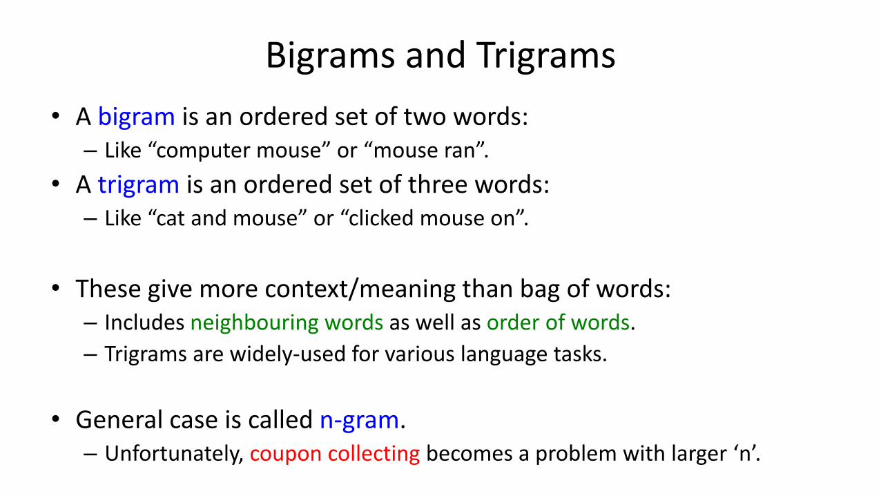
Bigrams and Trigrams

• A bigram is an ordered set of two words:– Like “computer mouse” or “mouse ran”.

• A trigram is an ordered set of three words:– Like “cat and mouse” or “clicked mouse on”.

• These give more context/meaning than bag of words:– Includes neighbouring words as well as order of words.

– Trigrams are widely-used for various language tasks.

• General case is called n-gram.– Unfortunately, coupon collecting becomes a problem with larger ‘n’.

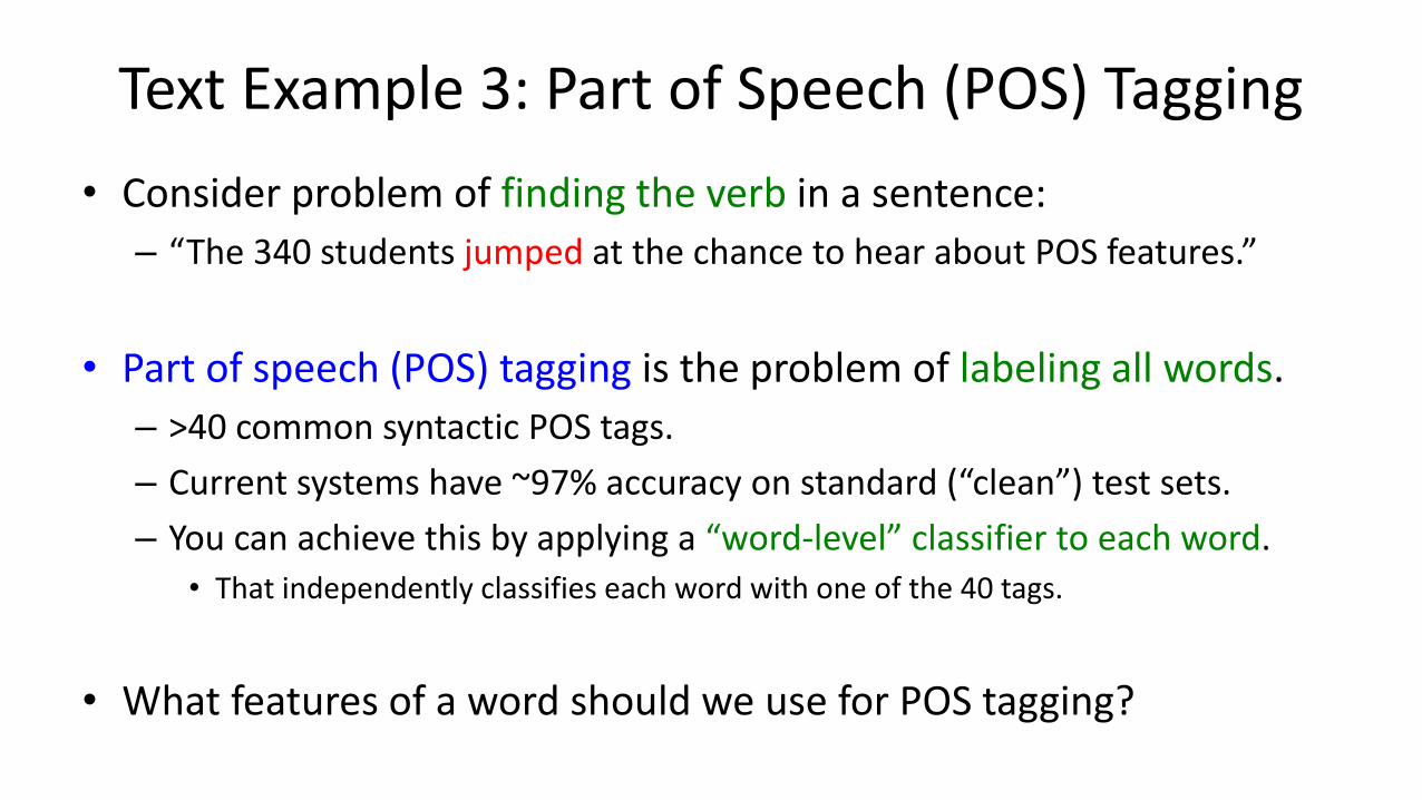
Text Example 3: Part of Speech (POS) Tagging

• Consider problem of finding the verb in a sentence:

– “The 340 students jumped at the chance to hear about POS features.”

• Part of speech (POS) tagging is the problem of labeling all words.

– >40 common syntactic POS tags.

– Current systems have ~97% accuracy on standard (“clean”) test sets.

– You can achieve this by applying a “word-level” classifier to each word.

• That independently classifies each word with one of the 40 tags.

• What features of a word should we use for POS tagging?

POS Features• Regularized multi-class logistic regression with these 19 features gives ~97% accuracy:

– Categorical features whose domain is all words (“lexical” features):• The word (e.g., “jumped” is usually a verb).• The previous word (e.g., “he” hit vs. “a” hit).• The previous previous word.• The next word.• The next next word.

– Categorical features whose domain is combinations of letters (“stem” features):• Prefix of length 1 (“what letter does the word start with?”)• Prefix of length 2.• Prefix of length 3.• Prefix of length 4 (“does it start with JUMP?”)• Suffix of length 1.• Suffix of length 2.• Suffix of length 3 (“does it end in ING?”)• Suffix of length 4.

– Binary features (“shape” features):• Does word contain a number?• Does word contain a capital?• Does word contain a hyphen?

Ordinal Features

• Categorical features with an ordering are called ordinal features.

• If using decision trees, makes sense to replace with numbers.– Captures ordering between the ratings.

– A rule like (rating ≥ 3) means (rating ≥ Good), which make sense.

Rating

Bad

Very Good

Good

Good

Very Bad

Good

Medium

Rating

2

5

4

4

1

4

3

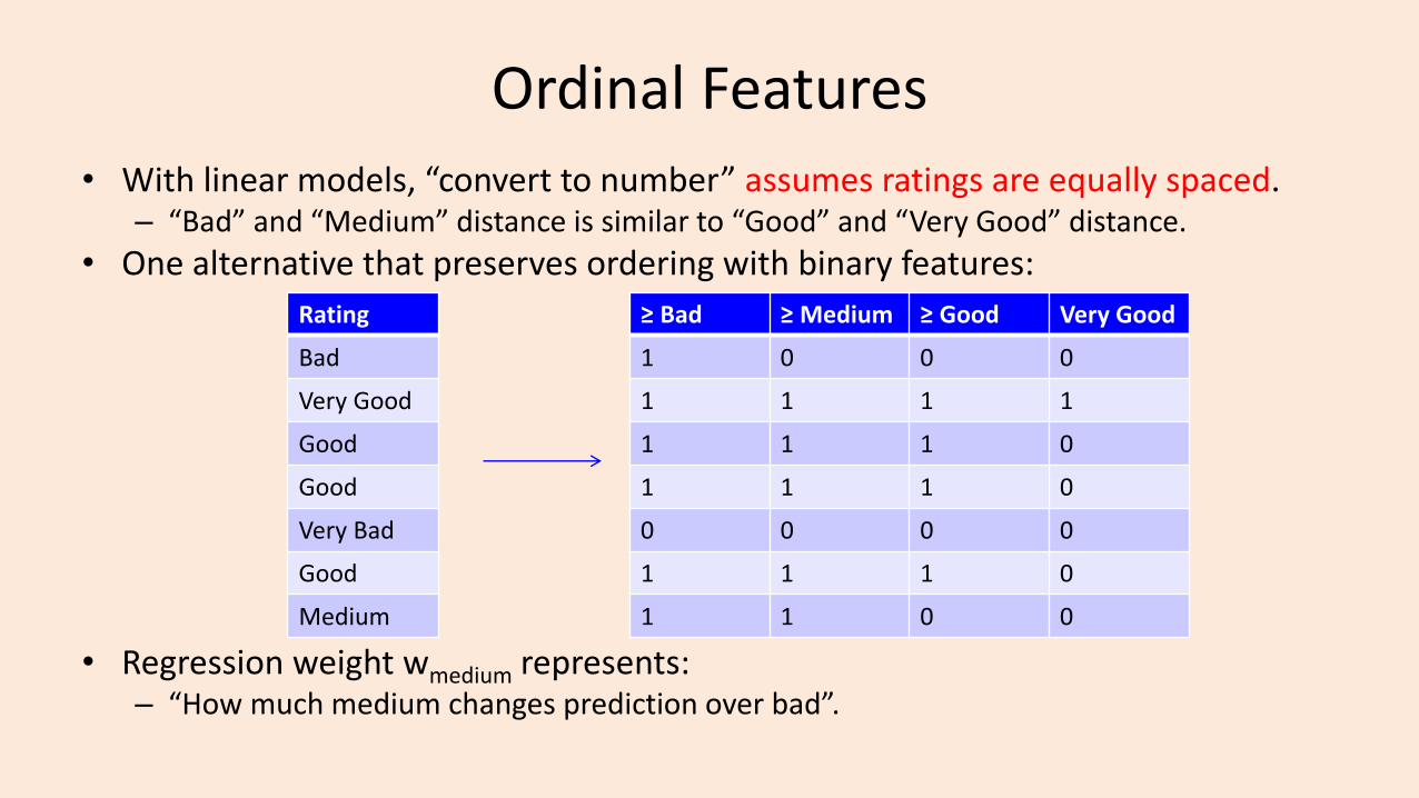
Ordinal Features

• With linear models, “convert to number” assumes ratings are equally spaced.– “Bad” and “Medium” distance is similar to “Good” and “Very Good” distance.

• One alternative that preserves ordering with binary features:

• Regression weight wmedium represents: – “How much medium changes prediction over bad”.

Rating

Bad

Very Good

Good

Good

Very Bad

Good

Medium

≥ Bad ≥ Medium ≥ Good Very Good

1 0 0 0

1 1 1 1

1 1 1 0

1 1 1 0

0 0 0 0

1 1 1 0

1 1 0 0

(pause)

Motivation: “Personalized” Important E-mails

• Features: bad of words, trigrams, regular expressions, and so on.

• There might be some “globally” important messages:

– “This is your mother, something terrible happened, give me a call ASAP.”

• But your “important” message may be unimportant to others.

– Similar for spam: “spam” for one user could be “not spam” for another.

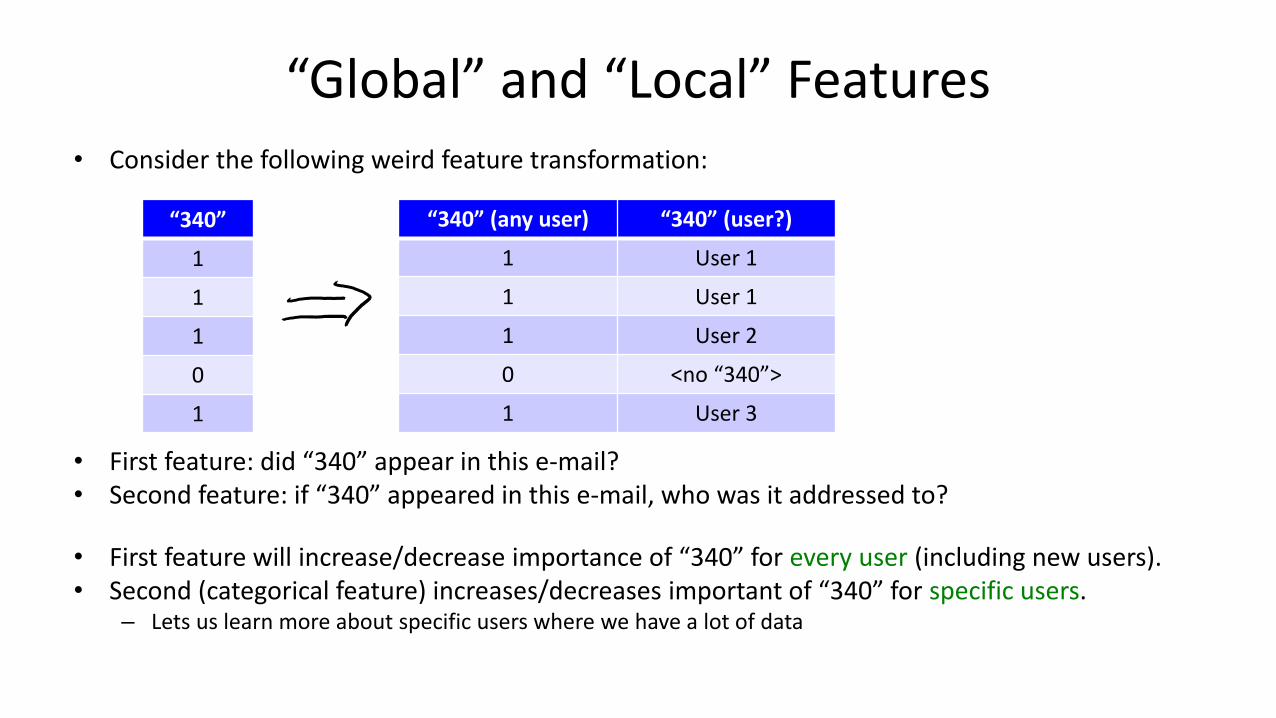
“Global” and “Local” Features• Consider the following weird feature transformation:

• First feature: did “340” appear in this e-mail?• Second feature: if “340” appeared in this e-mail, who was it addressed to?

• First feature will increase/decrease importance of “340” for every user (including new users).• Second (categorical feature) increases/decreases important of “340” for specific users.

– Lets us learn more about specific users where we have a lot of data

“340” (any user) “340” (user?)

1 User 1

1 User 1

1 User 2

0 <no “340”>

1 User 3

“340”

1

1

1

0

1

“Global” and “Local” Features

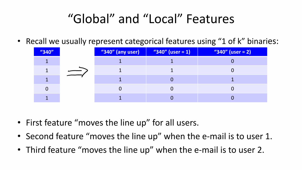
• Recall we usually represent categorical features using “1 of k” binaries:

• First feature “moves the line up” for all users.

• Second feature “moves the line up” when the e-mail is to user 1.

• Third feature “moves the line up” when the e-mail is to user 2.

“340” (any user) “340” (user = 1) “340” (user = 2)

1 1 0

1 1 0

1 0 1

0 0 0

1 0 0

“340”

1

1

1

0

1

The Big Global/Local Feature Table for E-mails

• Each row is one e-mail (there are lots of rows):

Summary

• Softmax loss is a multi-class version of logistic loss.

• Feature engineering can be a key factor affecting performance.

– Good features depend on the task and the model.

• Bag of words: not a good representation in general.

– But good features if word order isn’t needed to solve problem.

• Text features (beyond bag of words): trigrams, lexical, stem, shape.

– Try to capture important invariances in text data.

• Global vs. local features allow “personalized” predictions.

• Next time: feature engineering for image and sound data.

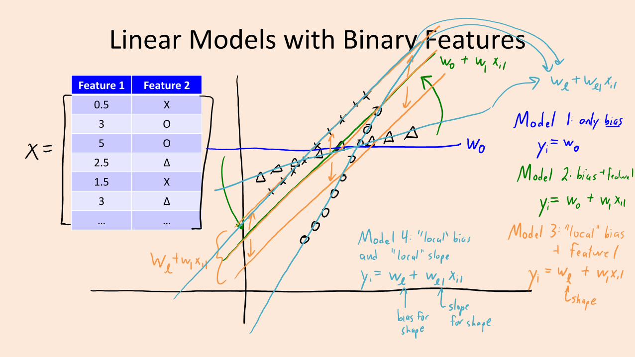
Linear Models with Binary Features

Feature 1 Feature 2

0.5 X

3 O

5 O

2.5 Δ

1.5 X

3 Δ

… …

Linear Models with Binary Features

Feature 1 Feature 2

0.5 X

3 O

5 O

2.5 Δ

1.5 X

3 Δ

… …

Linear Models with Binary Features

Feature 1 Feature 2

0.5 X

3 O

5 O

2.5 Δ

1.5 X

3 Δ

… …

Linear Models with Binary Features

Feature 1 Feature 2

0.5 X

3 O

5 O

2.5 Δ

1.5 X

3 Δ

… …

Linear Models with Binary Features

Feature 1 Feature 2

0.5 X

3 O

5 O

2.5 Δ

1.5 X

3 Δ

… …

Linear Models with Binary Features

Feature 1 Feature 2

0.5 X

3 O

5 O

2.5 Δ

1.5 X

3 Δ

… …