CPSC 340:Machine Learning and Data Mining

Principal Component Analysis

Fall 2015

Admin

• Midterm on Friday.

– Assignment 3 solutions posted after class.

– Practice midterm posted.

– List of topics posted.

– In class, 55 minutes, closed-book, cheat sheet: 2-pages each double-sided.

http://www.october212015.com/

Last time: Stochastic Gradient Methods

• We want to fit a regression model:

• If ‘g’ and ‘r’ are smooth, gradient descent allows huge ‘d’.

• When ‘n’ is huge/infinite, we can use stochastic gradient:

• For convergence, αt must go to zero.

• Amazing theoretical properties in terms of test error:– Even for non-IID data, but in practice often doesn’t live up to expectations.

• Nevertheless, widely-used because it allows enormous datasets.

The Story So Far…

• Supervised Learning Part 1:– Methods based on counting and distances.– Training vs. testing, parametric vs. non-parametric, ensemble methods.– Fundamental trade-off, no free lunch.

• Unsupervised Learning Part 1:– Methods based on counting and distances.– Clustering and association rules.

• Supervised Learning Part 2:– Methods based on linear models and gradient descent.– Continuity of predictions, suitability for high-dimensional problems. – Loss functions, change of basis, regularization, features selection, big problems.

• Unsupervised Learning Part 2:– Methods based on linear models and gradient descent.

Unsupervised Learning Part 2

• Unsupervised learning:

– We only have xi values, and want to do ‘something’ with them.

• Some unsupervised learning tasks:

– Clustering: What types of xi are there?

– Association rules: Which xij occur together?

– Outlier detection: Is this a ‘normal’ xi?

– Data visualization: What does the high-dimensional X look like?

– Ranking: Which are the most important xi?

– Latent-factors: What ‘parts’ are the xi made from?

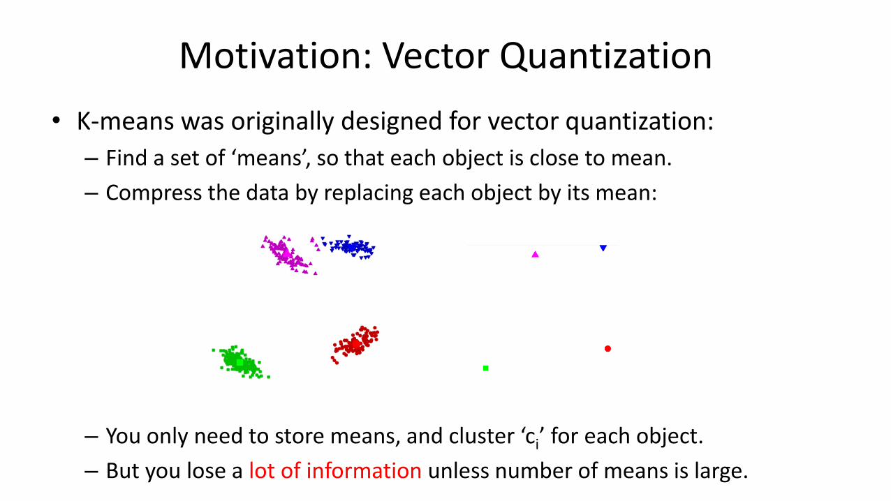
Motivation: Vector Quantization

• K-means was originally designed for vector quantization:

– Find a set of ‘means’, so that each object is close to mean.

– Compress the data by replacing each object by its mean:

– You only need to store means, and cluster ‘ci’ for each object.

– But you lose a lot of information unless number of means is large.

Latent-Factor Models

• Latent-factor models:– We don’t call them ‘means’ µc, we call them factors wc.– Approximate each object as a linear combination of factors:

– We still have ‘k’ by ‘d’ matrix ‘W’ of factors/means.– Instead of cluster ‘ci’, we have ‘k’ by ‘1’ weight vector ‘zi’ for each ‘I’.– K-means: special case where each (zi = 1) for ‘ci’ and (zi = 0) zero otherwise.

• Matrix inner factorization notation:

• Compresses if ‘k’ is much smaller than ‘d’.– Above assumes features have been standardized (otherwise, need bias).

Principal Component Analysis

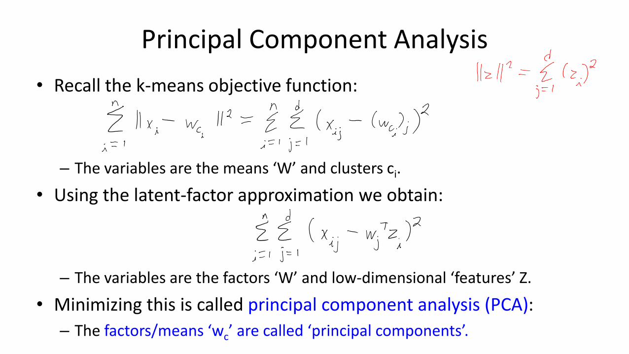
• Recall the k-means objective function:

– The variables are the means ‘W’ and clusters ci.

• Using the latent-factor approximation we obtain:

– The variables are the factors ‘W’ and low-dimensional ‘features’ Z.

• Minimizing this is called principal component analysis (PCA):

– The factors/means ‘wc’ are called ‘principal components’.

– Dimensionality reduction: replace ‘X’ with lower-dimensional ‘Z’.

– Outlier detection: if PCA gives poor approximation of xi, could be ‘outlier’.

– Basis for linear models: use ‘Z’ as features in regression models.

PCA Applications

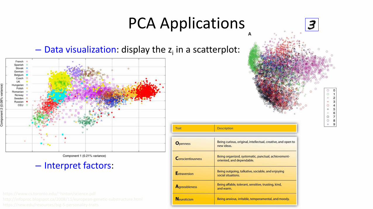
– Data visualization: display the zi in a scatterplot:

– Interpret factors:

https://www.cs.toronto.edu/~hinton/science.pdfhttp://infoproc.blogspot.ca/2008/11/european-genetic-substructure.htmlhttps://new.edu/resources/big-5-personality-traits

PCA Applications

Maximizing Variance vs. Minimizing Error

• PCA has been reinvented many times:

• There are many ways to arrive at the same model:– Classic ‘analysis’ view: PCA maximizes variance in compressed space.

• You pick the ‘wc’ to explain as much variance as possible.

– We take the ‘synthesis’ view: PCA minimizes error of approximation.• Makes connection to k-means and least squares.

• We can use tricks from linear regression to fix PCA’s many problems.

https://en.wikipedia.org/wiki/Principal_component_analysis

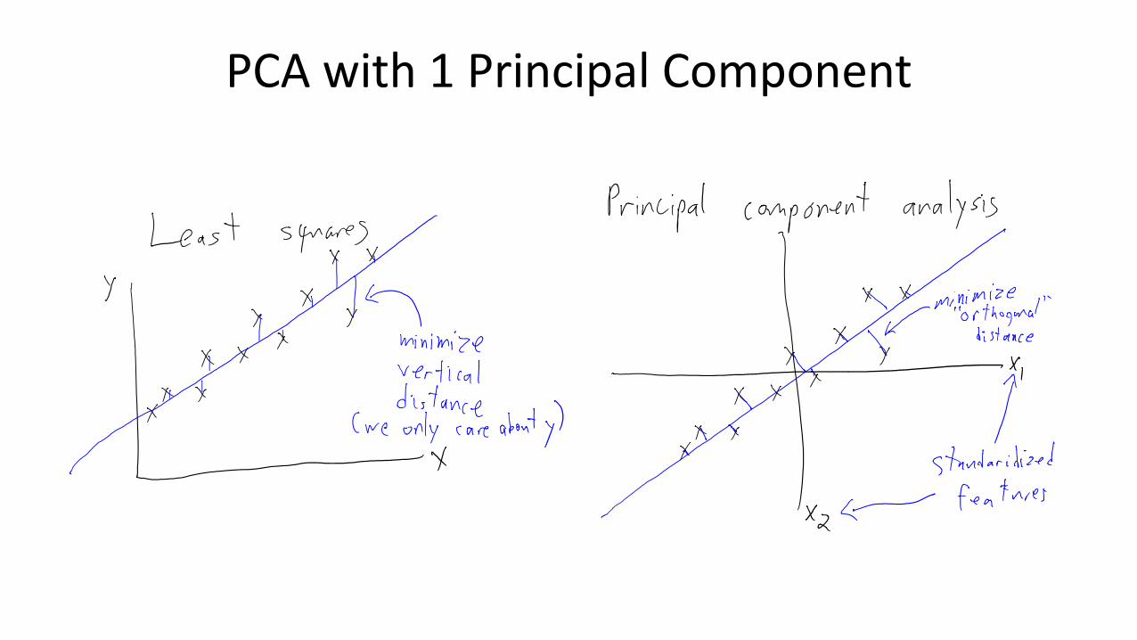
PCA with 1 Principal Component

• PCA with one principal component (PC) ‘w’:

• Very similar to a least squares problem, but note that:– We have no ‘yi’, we are trying to predict each vector feature xij from the zi.

– Latent feaures ‘zi’ are also variables, we are learning the zi too.(if you know the zi, equivalent to least squares)

PCA with 1 Principal Component

PCA with 1 Principal Component

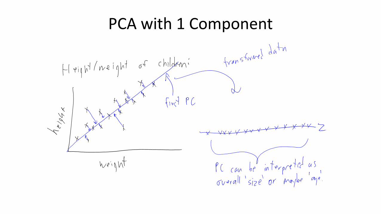
PCA with 1 Component

PCA with 1 Component

• Our PCA objective function with one PC:

• For small problems use closed-form solution:

– First ‘right singular vector’ of X is a solution.

– Equivalently, eigenvector of XTX with largest eigenvalue.

• For problems where ‘d’ is large, alternating minimization:

– Update w given the zi, then update the zi given w (similar to k-means)

– Convex in w, convex in zi, but not jointly convex.

– But, only stable local minimum is a global minimum.

• When ‘n’ is large, recent provably-correct stochastic gradient methods.

PCA with 1 Component

• Our PCA objective function with one PC:

• Even with 1 PC, solution is never unique:

• To address this issue, we usually put a constraint on ‘w’:

• For iterative methods, can do this afterwards (then update the zi).

General PCA

• Our general PCA framework:

• General objective function:

• Same solution methods (closed-form is top ‘k’ singular vectors).

• With multiple components, even directions are not unique.

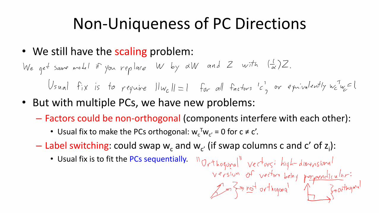
Non-Uniqueness of PC Directions

• We still have the scaling problem:

• But with multiple PCs, we have new problems:

– Factors could be non-orthogonal (components interfere with each other):

• Usual fix to make the PCs orthogonal: wcTwc’ = 0 for c ≠ c’.

– Label switching: could swap wc and wc’ (if swap columns c and c’ of zi):

• Usual fix is to fit the PCs sequentially.

Basis, Orthogonality, Sequential Fitting

Basis, Orthogonality, Sequential Fitting

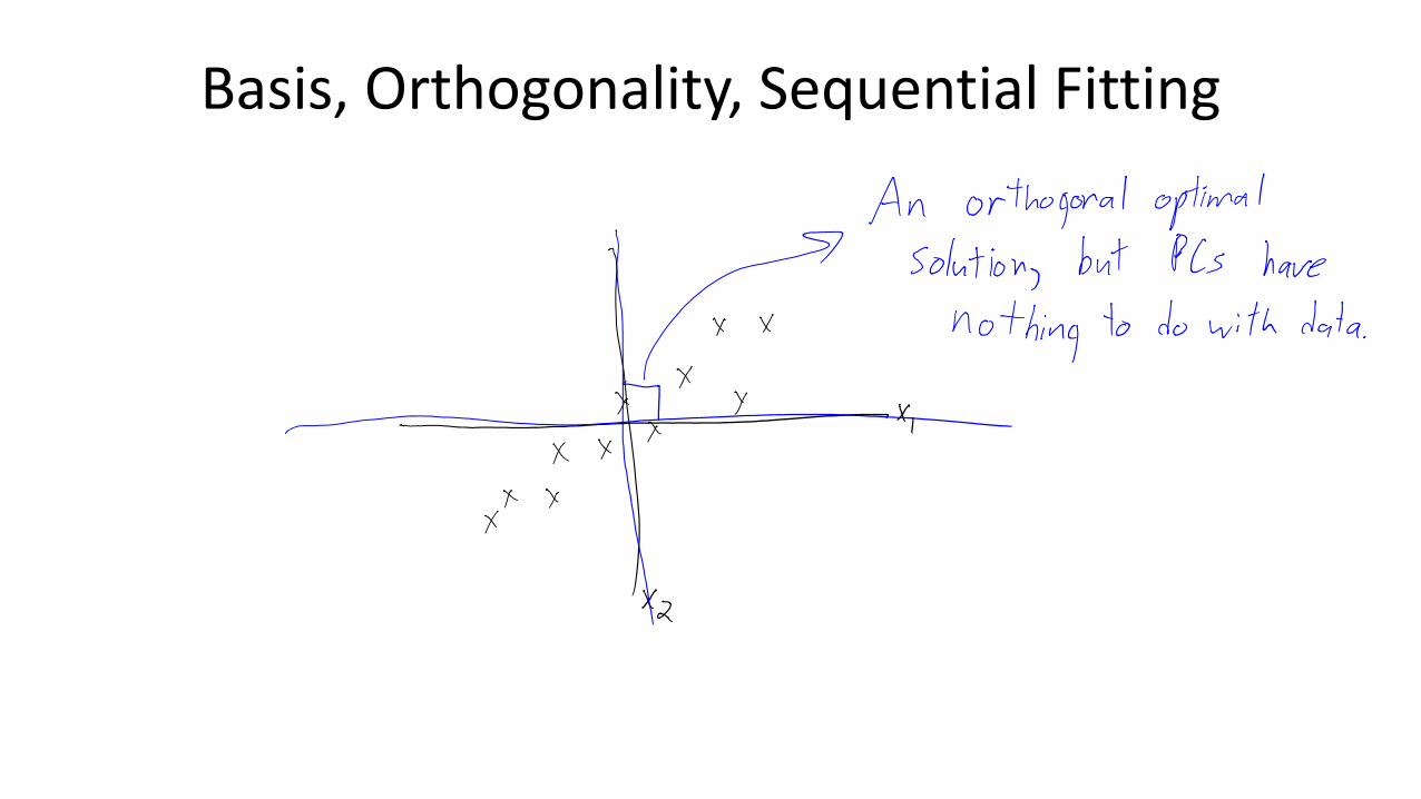
Basis, Orthogonality, Sequential Fitting

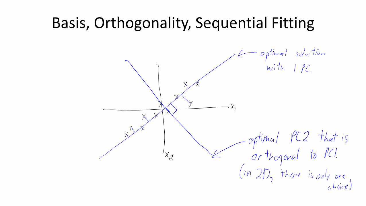
Basis, Orthogonality, Sequential Fitting

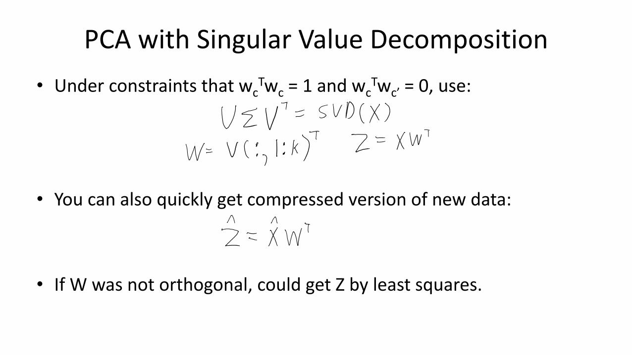
PCA with Singular Value Decomposition

• Under constraints that wcTwc = 1 and wc

Twc’ = 0, use:

• You can also quickly get compressed version of new data:

• If W was not orthogonal, could get Z by least squares.

Application: Face Detection

• ‘Eigenfaces’ classically used as basis for face detection:

http://mikedusenberry.com/on-eigenfaces/

Summary

• Latent-factor models compress data as linear combination of ‘factors’.

• Principal component analysis: most common variant based on squared reconstruction error.

• Orthogonal basis is useful for interpretation and identifying of PCs.

• Next time: the discovering a hole in the ozone layer.