Embed Size (px)
Citation preview

Covariance function estimation in Gaussian process regression
François Bachoc
Department of Statistics and Operations Research, University of Vienna
WU Research Seminar - May 2015
François Bachoc Gaussian process regression WU - May 2015 1 / 46

1 Gaussian process regression
2 Maximum Likelihood and Cross Validation for covariance function estimation
3 Asymptotic analysis of the well-specified case
4 Finite-sample and asymptotic analysis of the misspecified case
François Bachoc Gaussian process regression WU - May 2015 2 / 46
Gaussian process regression
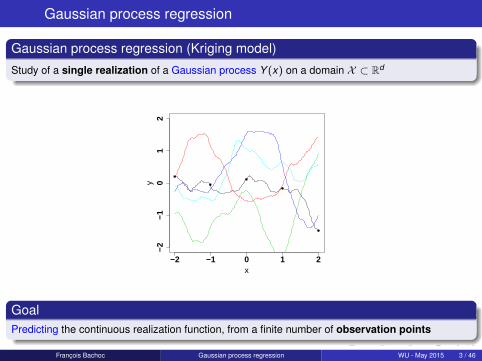
Gaussian process regression (Kriging model)
Study of a single realization of a Gaussian process Y (x) on a domain X ⊂ Rd
−2 −1 0 1 2
−2−1
01
2
x
y
GoalPredicting the continuous realization function, from a finite number of observation points
François Bachoc Gaussian process regression WU - May 2015 3 / 46
The Gaussian process
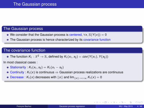
The Gaussian processWe consider that the Gaussian process is centered, ∀x ,E(Y (x)) = 0
The Gaussian process is hence characterized by its covariance function
The covariance functionThe function K1 : X 2 → R, defined by K1(x1, x2) = cov(Y (x1),Y (x2))
In most classical cases :
Stationarity : K1(x1, x2) = K1(x1 − x2)
Continuity : K1(x) is continuous⇒ Gaussian process realizations are continuous
Decrease : K1(x) decreases with ||x || and lim||x||→+∞ K1(x) = 0
François Bachoc Gaussian process regression WU - May 2015 4 / 46

Example of the Matérn 32 covariance function on R
The Matérn 32 covariance function, for a Gaussian
process on R is parameterized by
A variance parameter σ2 > 0
A correlation length parameter ` > 0
It is defined as
Kσ2,`(x1, x2) = σ2(
1 +√
6|x1 − x2|
`
)e−√
6|x1−x2|`
0 1 2 3 4
0.0
0.2
0.4
0.6
0.8
1.0
x
cov
l=0.5l=1l=2
InterpretationStationarity, continuity, decrease
σ2 corresponds to the order of magnitude of the functions that are realizations of theGaussian process
` corresponds to the speed of variation of the functions that are realizations of the Gaussianprocess
⇒ Natural generalization on Rd
François Bachoc Gaussian process regression WU - May 2015 5 / 46

Covariance function estimation
ParameterizationCovariance function model
{σ2Kθ, σ2 ≥ 0, θ ∈ Θ
}for the Gaussian process Y .
σ2 is the variance parameter
θ is the multidimensional correlation parameter. Kθ is a stationary correlation function
ObservationsY is observed at x1, ..., xn ∈ X , yielding the Gaussian vector y = (Y (x1), ...,Y (xn))
Estimation
Objective : build estimators σ2(y) and θ(y)
François Bachoc Gaussian process regression WU - May 2015 6 / 46

Prediction with estimated covariance function
Gaussian process Y observed at x1, ..., xn and predicted at xnewy = (Y (x1), ...,Y (xn))t
Once the covariance parameters have been estimated and fixed to σ and θ
Rθ is the correlation matrix of Y at x1, ..., xn under correlation function Kθrθ is the correlation vector of Y between x1, ..., xn and xnew under correlation function Kθ
Prediction
The prediction is Yθ(xnew ) := Eθ(Y (xnew )|Y (x1), ...,Y (xn)) = r tθR−1θ
y .
Predictive varianceThe predictive variance isvarσ,θ(Y (xnew )|Y (x1), ...,Y (xn)) = Eσ,θ
[(Y (xnew )− Yθ(xnew ))2
]= σ2
(1− r t
θR−1θ
rθ)
.
("Plug-in" approach)
François Bachoc Gaussian process regression WU - May 2015 7 / 46
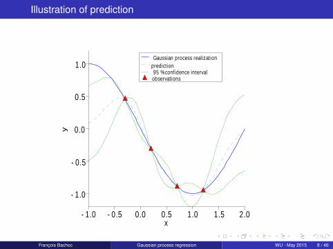
Illustration of prediction
- 1.0
- 0.5
0.0
0.5
1.0
- 1.0 - 0.5 0.0 0.5 1.0 1.5 2.0x
yGaussian process realizat ion
predict ion95 % confidence intervalobservat ions
François Bachoc Gaussian process regression WU - May 2015 8 / 46

Application to computer experiments
Computer modelA computer model, computing a given variable of interest, corresponds to a deterministic functionRd → R. Evaluations of this function are time consuming
Examples : Simulation of a nuclear fuel pin, of thermal-hydraulic systems, of components of acar, of a plane...
Gaussian process model for computer experimentsBasic idea : representing the code function by a realization of a Gaussian process
Bayesian framework on a fixed function
What we obtainMetamodel of the code : the Gaussian process prediction function approximates the codefunction, and its evaluation cost is negligible
Error indicator with the predictive variance
Full conditional Gaussian process⇒ possible goal-oriented iterative strategies foroptimization, failure domain estimation, small probability problems, code calibration...
François Bachoc Gaussian process regression WU - May 2015 9 / 46

Conclusion
Gaussian process regression :
The covariance function characterizes the Gaussian process
It is estimated first (main topic of the talk, cf below)
Then we can compute prediction and predictive variances with explicit matrix vector formulas
Widely used for computer experiments
François Bachoc Gaussian process regression WU - May 2015 10 / 46
1 Gaussian process regression
2 Maximum Likelihood and Cross Validation for covariance function estimation
3 Asymptotic analysis of the well-specified case
4 Finite-sample and asymptotic analysis of the misspecified case
François Bachoc Gaussian process regression WU - May 2015 11 / 46
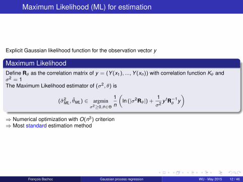
Maximum Likelihood (ML) for estimation
Explicit Gaussian likelihood function for the observation vector y
Maximum LikelihoodDefine Rθ as the correlation matrix of y = (Y (x1), ...,Y (xn)) with correlation function Kθ andσ2 = 1The Maximum Likelihood estimator of (σ2, θ) is
(σ2ML, θML) ∈ argmin
σ2≥0,θ∈Θ
1n
(ln (|σ2Rθ|) +
1σ2
y t R−1θ y
)
⇒ Numerical optimization with O(n3) criterion⇒ Most standard estimation method
François Bachoc Gaussian process regression WU - May 2015 12 / 46

Cross Validation (CV) for estimation
yθ,i,−i = Eθ(Y (xi )|y1, ..., yi−1, yi+1, ..., yn)
σ2c2θ,i,−i = varσ2,θ(Y (xi )|y1, ..., yi−1, yi+1, ..., yn)
Leave-One-Out criteria we study
θCV ∈ argminθ∈Θ
n∑i=1
(yi − yθ,i,−i )2
and1n
n∑i=1
(yi − yθCV ,i,−i )2
σ2CV c2
θCV ,i,−i
= 1⇔ σ2CV =
1n
n∑i=1
(yi − yθCV ,i,−i )2
c2θCV ,i,−i
=⇒ Alternative method used by some authors
François Bachoc Gaussian process regression WU - May 2015 13 / 46

Virtual Leave One Out formula
Let Rθ be the correlation matrix of y = (y1, ..., yn) with correlation function Kθ
Virtual Leave-One-Out
yi − yθ,i,−i =1
(R−1θ )i,i
(R−1θ y
)i
and c2θ,i,−i =
1
(R−1θ )i,i
O. Dubrule, Cross Validation of Kriging in a Unique Neighborhood, Mathematical Geology,1983.
Using the virtual Cross Validation formula :
θCV ∈ argminθ∈Θ
1n
y t R−1θ diag(R−1
θ )−2R−1θ y
andσ2
CV =1n
y t R−1θCV
diag(R−1θCV
)−1R−1θCV
y
⇒ Same computational cost as ML
François Bachoc Gaussian process regression WU - May 2015 14 / 46
1 Gaussian process regression
2 Maximum Likelihood and Cross Validation for covariance function estimation
3 Asymptotic analysis of the well-specified case
4 Finite-sample and asymptotic analysis of the misspecified case
François Bachoc Gaussian process regression WU - May 2015 15 / 46

Well-specified case
Estimation of θ only
For simplicity, we do not distinguish the estimations of σ2 and θ. Hence we use the set{Kθ, θ ∈ Θ} of stationary covariance functions for the estimation.
Well-specified modelThe true covariance function K1 of the Gaussian process belongs to the set {Kθ, θ ∈ Θ}. Hence
K1 = Kθ0 , θ0 ∈ Θ
=⇒ Most standard theoretical framework for estimation=⇒ ML and CV estimators can be analyzed and compared w.r.t. estimation error criteria ( basedon |θ − θ0|)
François Bachoc Gaussian process regression WU - May 2015 16 / 46
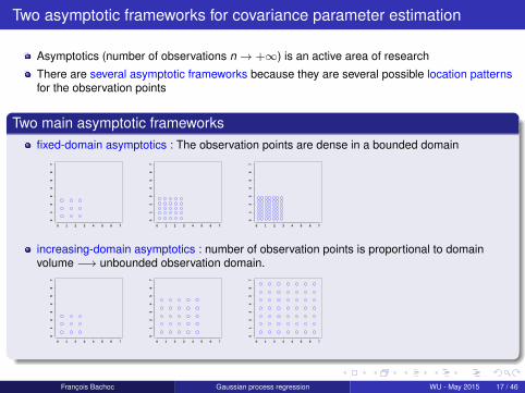
Two asymptotic frameworks for covariance parameter estimation
Asymptotics (number of observations n→ +∞) is an active area of research
There are several asymptotic frameworks because they are several possible location patternsfor the observation points
Two main asymptotic frameworksfixed-domain asymptotics : The observation points are dense in a bounded domain
0 1 2 3 4 5 6 7
01
23
45
67
0 1 2 3 4 5 6 7
01
23
45
67
0 1 2 3 4 5 6 7
01
23
45
67
increasing-domain asymptotics : number of observation points is proportional to domainvolume −→ unbounded observation domain.
0 1 2 3 4 5 6 7
01
23
45
67
0 1 2 3 4 5 6 7
01
23
45
67
0 1 2 3 4 5 6 7
01
23
45
67
François Bachoc Gaussian process regression WU - May 2015 17 / 46

Existing fixed-domain asymptotic results
From 80’-90’ and onward. Fruitful theory for interaction estimation-prediction.
Stein M, Interpolation of Spatial Data : Some Theory for Kriging, Springer, New York,1999.
Consistent estimation is impossible for some covariance parameters (identifiable infinite-sample), see e.g.
Zhang, H., Inconsistent Estimation and Asymptotically Equivalent Interpolations inModel-Based Geostatistics, Journal of the American Statistical Association (99),250-261, 2004.
Proofs (consistency, asymptotic distribution) are challenging in several waysThey are done on a case-by-case basis for the covariance modelsThey may assume gridded observation points
No impact of spatial sampling of observation points on asymptotic distribution
(No results for CV)
François Bachoc Gaussian process regression WU - May 2015 18 / 46

Existing increasing-domain asymptotic results
Consistent estimation is possible for all covariance parameters (that are identifiable infinite-sample). [More independence between observations]
Asymptotic normality proved for Maximum-Likelihood
Mardia K, Marshall R, Maximum likelihood estimation of models for residual covariancein spatial regression, Biometrika 71 (1984) 135-146.
N. Cressie and S.N Lahiri, The asymptotic distribution of REML estimators, Journal ofMultivariate Analysis 45 (1993) 217-233.
N. Cressie and S.N Lahiri, Asymptotics for REML estimation of spatial covarianceparameters, Journal of Statistical Planning and Inference 50 (1996) 327-341.
Under conditions that areGeneral for the covariance modelNot simple to check or specific for the spatial sampling
(No results for CV)
=⇒We study increasing-domain asymptotics for ML and CV
François Bachoc Gaussian process regression WU - May 2015 19 / 46
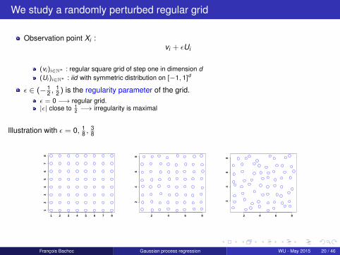
We study a randomly perturbed regular grid
Observation point Xi :vi + εUi
(vi )i∈N∗ : regular square grid of step one in dimension d(Ui )i∈N∗ : iid with symmetric distribution on [−1, 1]d
ε ∈ (− 12 ,
12 ) is the regularity parameter of the grid.
ε = 0 −→ regular grid.|ε| close to 1
2 −→ irregularity is maximal
Illustration with ε = 0, 18 ,
38
1 2 3 4 5 6 7 8
12
34
56
78
2 4 6 8
24
68
2 4 6 8
24
68
François Bachoc Gaussian process regression WU - May 2015 20 / 46
Why a randomly perturbed regular grid ?
Realizations car correspond to various sampling techniques for the observation points
In the corresponding paper, one main objective is to study the impact of the irregularity(regularity parameter ε) :
F. Bachoc, Asymptotic analysis of the role of spatial sampling for covariance parameterestimation of Gaussian processes, Journal of Multivariate Analysis 125 (2014) 1-35.
Note the condition |ε| < 1/2 =⇒ minimum distance between observation points =⇒technically convenient and appears in aforementioned publications
François Bachoc Gaussian process regression WU - May 2015 21 / 46
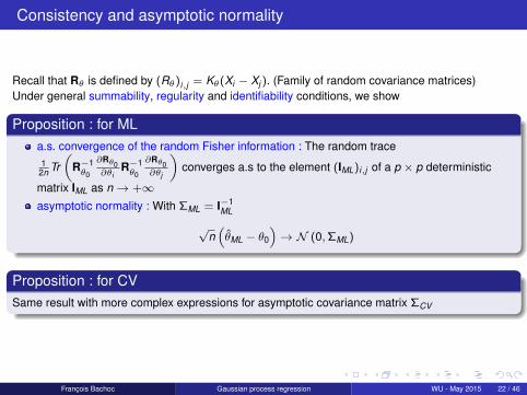
Consistency and asymptotic normality
Recall that Rθ is defined by (Rθ)i,j = Kθ(Xi − Xj ). (Family of random covariance matrices)Under general summability, regularity and identifiability conditions, we show
Proposition : for MLa.s. convergence of the random Fisher information : The random trace1
2n Tr(
R−1θ0
∂Rθ0∂θi
R−1θ0
∂Rθ0∂θj
)converges a.s to the element (IML)i,j of a p × p deterministic
matrix IML as n→ +∞asymptotic normality : With ΣML = I−1
ML
√n(θML − θ0
)→ N (0,ΣML)
Proposition : for CVSame result with more complex expressions for asymptotic covariance matrix ΣCV
François Bachoc Gaussian process regression WU - May 2015 22 / 46

Conclusion on well-specified case
In this expansion-domain asymptotic framework
ML and CV are consistent and have the standard rate of convergence√
n
(not presented here) in the corresponding paper we show, numerically, than CV has a largerasymptotic variance =⇒ could be expected since we address the well-specified case
(not presented here) in the paper we study numerically the impact of irregularity of spatialsampling on asymptotic variance =⇒ irregular sampling is beneficial to estimation
François Bachoc Gaussian process regression WU - May 2015 23 / 46

1 Gaussian process regression
2 Maximum Likelihood and Cross Validation for covariance function estimation
3 Asymptotic analysis of the well-specified case
4 Finite-sample and asymptotic analysis of the misspecified case
François Bachoc Gaussian process regression WU - May 2015 24 / 46
Misspecified case
The covariance function K1 of Y does not belong to{σ2Kθ, σ2 ≥ 0, θ ∈ Θ
}=⇒ There is no true covariance parameter but there may be optimal covariance parameters fordifference criteria :
prediction mean square error
confidence interval reliability
multidimensional Kullback-Leibler distance
...
=⇒ Cross Validation can be more appropriate than Maximum Likelihood for some of these criteria
François Bachoc Gaussian process regression WU - May 2015 25 / 46
Finite-sample analysis
We proceed in two steps
When covariance function model is{σ2K2, σ
2 ≥ 0}
, with K2 a fixed correlation function, andK1 is the true covariance function : explicit expressions and numerical tests
In the general case : numerical studies
Bachoc F, Cross Validation and Maximum Likelihood estimations of hyper-parameters ofGaussian processes with model misspecification, Computational Statistics and Data Analysis66 (2013) 55-69.
François Bachoc Gaussian process regression WU - May 2015 26 / 46

Case of variance parameter estimation
Ynew : prediction of Ynew := Y (xnew ) with fixed misspecified correlation function K2
E[
(Ynew − Ynew )2∣∣∣ y] : conditional mean square error of the prediction Ynew
One estimates σ2 by σ2. σ2 may be σ2ML or σ2
CV
Conditional mean square error of Ynew predicted by σ2c2xnew with c2
xnew fixed by K2
Definition : the RiskWe study the Risk criterion for an estimator σ2 of σ2
Rσ2,xnew= E
[(E[
(Ynew − Ynew )2∣∣∣ y]− σ2c2
xnew
)2]
François Bachoc Gaussian process regression WU - May 2015 27 / 46

Explicit expression of the Risk
Let, for i = 1, 2 :
ri be the covariance vector of Y between x1, ..., xn and xnew with covariance function Ki
Ri be the covariance matrix of Y at x1, ..., xn with covariance function Ki
Proposition : formula for quadratic estimators
When σ2 = y t My , we have
Rσ2,xnew= f (M0,M0) + 2c1tr(M0)− 2c2f (M0,M1)
+c21 − 2c1c2tr(M1) + c2
2 f (M1,M1)
with
f (A,B) = tr(A)tr(B) + 2tr(AB)
M0 = (R−12 r2 − R−1
1 r1)(r t2R−1
2 − r t1R−1
1 )R1
M1 = MR1
ci = 1− r ti R−1
i ri , i = 1, 2
Corollary : ML and CV are quadratic estimators =⇒ we can carry out an exhaustive numericalstudy of the Risk criterion
François Bachoc Gaussian process regression WU - May 2015 28 / 46

Two criteria for the numerical study
Definition : Risk on Target Ratio (RTR)
RTR(xnew ) =
√Rσ2,xnew
E[(Ynew − Ynew )2
] =
√√√√E
[(E[(
Ynew − Ynew
)2∣∣∣∣ y]− σ2c2
xnew
)2]
E[(Ynew − Ynew )2
]
Definition : Bias on Target Ratio (BTR)
BTR(xnew ) =
∣∣∣E [(Ynew − Ynew )2]− E
(σ2c2
xnew
)∣∣∣E[(Ynew − Ynew )2
]Integrated versions over the prediction domain X
IRTR =
√∫X
RTR2(xnew )dxnew
and
IBTR =
√∫X
BTR2(xnew )dxnew
François Bachoc Gaussian process regression WU - May 2015 29 / 46

For designs of observation points that are not too regular (1/6)
70 observation points on [0, 1]5. Mean over LHS-Maximin samplings.K1 and K2 are power-exponential covariance functions,
Ki (x , y) = exp
− 5∑j=1
( |xj − yj |`i
)pi
,with `1 = `2 = 1.2, p1 = 1.5, and p2 varying.
François Bachoc Gaussian process regression WU - May 2015 30 / 46

For designs of observation points that are not too regular (2/6)
70 observations on [0, 1]5. Mean over LHS-Maximin samplings.K1 and K2 are power-exponential covariance functions,
Ki (x , y) = exp
− 5∑j=1
( |xj − yj |`i
)pi
,with `1 = `2 = 1.2, p1 = 1.5, and p2 varying.
François Bachoc Gaussian process regression WU - May 2015 31 / 46

For designs of observation points that are not too regular (3/6)
70 observations on [0, 1]5. Mean over LHS-Maximin samplings.K1 and K2 are Matérn covariance functions,
Ki (x , y) =1
Γ(νi )2νi−1
(2√νi||x − y ||2
`i
)νiKνi
(2√νi||x − y ||2
`i
),
with Γ the Gamma function and Kνi the modified Bessel function of second order.We use `1 = `2 = 1.2, ν1 = 1.5, and ν2 varying.
François Bachoc Gaussian process regression WU - May 2015 32 / 46

For designs of observation points that are not too regular (4/6)
70 observations on [0, 1]5. Mean over LHS-Maximin samplings.K1 and K2 are Matérn covariance functions,
Ki (x , y) =1
Γ(νi )2νi−1
(2√νi||x − y ||2
`i
)νiKνi
(2√νi||x − y ||2
`i
),
with Γ the Gamma function and Kνi the modified Bessel function of second order.We use `1 = `2 = 1.2, ν1 = 1.5, and ν2 varying.
François Bachoc Gaussian process regression WU - May 2015 33 / 46
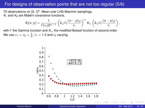
For designs of observation points that are not too regular (5/6)
70 observations on [0, 1]5. Mean over LHS-Maximin samplings.K1 and K2 are Matérn covariance functions,
Ki (x , y) =1
Γ(νi )2νi−1
(2√νi||x − y ||2
`i
)νiKνi
(2√νi||x − y ||2
`i
),
with Γ the Gamma function and Kνi the modified Bessel function of second order.We use ν1 = ν2 = 3
2 , `1 = 1.2 and `2 varying.
François Bachoc Gaussian process regression WU - May 2015 34 / 46

For designs of observation points that are not too regular (6/6)
70 observations on [0, 1]5. Mean over LHS-Maximin samplings.K1 and K2 are Matérn covariance functions,
Ki (x , y) =1
Γ(νi )2νi−1
(2√νi||x − y ||2
`i
)νiKνi
(2√νi||x − y ||2
`i
),
with Γ the Gamma function and Kνi the modified Bessel function of second order.We use ν1 = ν2 = 3
2 , `1 = 1.2 and `2 varying.
François Bachoc Gaussian process regression WU - May 2015 35 / 46

Case of a regular grid (Smolyak construction) (1/4)
Projections of the observations points on the first two base vectors :
0.1
0.2
0.3
0.4
0.5
0.6
0.7
0.8
0.9
0.1 0.2 0.3 0.4 0.5 0.6 0.7 0.8 0.9
François Bachoc Gaussian process regression WU - May 2015 36 / 46
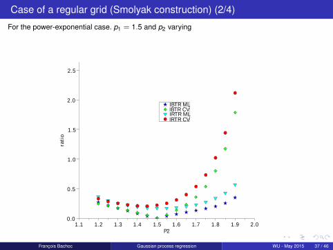
Case of a regular grid (Smolyak construction) (2/4)
For the power-exponential case. p1 = 1.5 and p2 varying
0.0
0.5
1.0
1.5
2.0
2.5
1.1 1.2 1.3 1.4 1.5 1.6 1.7 1.8 1.9 2.0P2
rati
o
IBTR MLIBTR CVIRTR MLIRTR CV
François Bachoc Gaussian process regression WU - May 2015 37 / 46

Case of a regular grid (Smolyak construction) (3/4)
For the Matérn case. ν1 = 1.5 and ν2 varying
0.0
0.5
1.0
1.5
2.0
2.5
3.0
0.5 1.0 1.5 2.0 2.5Nu2
rati
o
IBTR MLIBTR CVIRTR MLIRTR CV
François Bachoc Gaussian process regression WU - May 2015 38 / 46
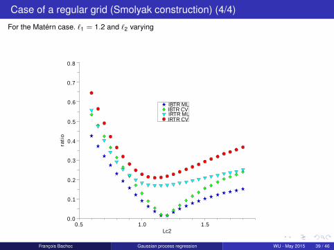
Case of a regular grid (Smolyak construction) (4/4)
For the Matérn case. `1 = 1.2 and `2 varying
0.0
0.1
0.2
0.3
0.4
0.5
0.6
0.7
0.8
0.5 1.0 1.5Lc2
rati
o
IBTR MLIBTR CVIRTR MLIRTR CV
François Bachoc Gaussian process regression WU - May 2015 39 / 46

Summary of finite-sample analysis
For variance parameter estimationFor not-too-regular designs : CV is more robust than ML to misspecification
Larger variance but smaller bias for CVThe bias term becomes dominant in the model misspecification case
For regular designs : CV is more biased than ML
=⇒ (not presented here) in the paper, a numerical study based on analytical functions confirmsthese findings for the estimation of correlation parameters as well
InterpretationFor irregular samplings of observations points, prediction for new points is similar toLeave-One-Out prediction =⇒ the Cross Validation criterion can be unbiased
For regular samplings of observations points, prediction for new points is different fromLeave-One-Out prediction =⇒ the Cross Validation criterion is biased
=⇒ we now support this interpretation in an asymptotic framework
François Bachoc Gaussian process regression WU - May 2015 40 / 46
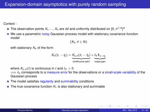
Expansion-domain asymptotics with purely random sampling
Context :
The observation points X1, ...,Xn are iid and uniformly distributed on [0, n1/d ]d
We use a parametric noisy Gaussian process model with stationary covariance functionmodel
{Kθ, θ ∈ Θ}
with stationary Kθ of the form
Kθ(t1 − t2) = Kc,θ(t1 − t2)︸ ︷︷ ︸continuous part
+ δθ1t1=t2︸ ︷︷ ︸noise part
where Kc,θ(t) is continuous in t and δθ > 0=⇒ δθ corresponds to a measure error for the observations or a small-scale variability of theGaussian process
The model satisfies regularity and summability conditions
The true covariance function K1 is also stationary and summable
François Bachoc Gaussian process regression WU - May 2015 41 / 46

Cross Validation asymptotically minimizes the integrated predictionerror (1/2)
Let Yθ(t) be the prediction of the Gaussian process Y at t , under correlation function Kθ , fromobservations Y (x1), ...,Y (xn)
Integrated prediction error :
En,θ :=1n
∫[0,n1/d ]d
(Yθ(t)− Y (t)
)2dt
Intuition :The variable t above plays the same role as a new observation point Xn+1, uniform on [0, n1/d ]d
and independent of X1, ...,Xn
So we haveE(En,θ
)= E
([Y (Xn+1)− Eθ|X (Y (Xn+1)|Y (X1), ...,Y (Xn))
]2)and so when n is large
E(En,θ
)≈ E
(1n
n∑i=1
(yi − yθ,i,−i )2
)=⇒ This is an indication that the Cross Validation estimator can be optimal for integratedprediction error
François Bachoc Gaussian process regression WU - May 2015 42 / 46

Cross Validation asymptotically minimizes the integrated predictionerror (2/2)
We show in
F. Bachoc, “Asymptotic analysis of covariance parameter estimation for Gaussian processesin the misspecified case”, ArXiv preprint http://arxiv.org/abs/1412.1926, Submitted.
TheoremWith
En,θ =
∫[0,n1/d ]d
(Yθ(t)− Y (t)
)2dt
we haveEn,θCV
= infθ∈Θ
En,θ + op(1).
Comments :
Same Gaussian process realization for both covariance parameter estimation and predictionerror
The optimal (unreachable) prediction error infθ∈Θ En,θ is lower-bounded =⇒ CV is indeedasymptotically optimal
François Bachoc Gaussian process regression WU - May 2015 43 / 46

Maximum Likelihood asymptotically minimizes the multidimensionalKullback-Leibler divergence
Let KLn,θ be 1/n times the Kullback-Leibler divergence dKL(K1||Kθ), between themultidimensional Gaussian distributions of y , given observation points X1, ...,Xn, under covariancefunctions Kθ and K1.We show
Theorem
KLn,θML= infθ∈Θ
KLn,θ + op(1).
Comments :
In increasing-domain asymptotics, when Kθ 6= K0, KLn,θ is usually lower-bounded =⇒ ML isindeed asymptotically optimal
Maximum Likelihood is optimal for a criterion that is not prediction oriented
François Bachoc Gaussian process regression WU - May 2015 44 / 46

Conclusion
The results shown support the following general picture
For well-specified models, ML would be optimal
For regular designs of observation points, the principle of CV does not really have ground
For more irregular designs of observation points, CV can be preferable for specificprediction-purposes (e.g. integrated prediction error). (But its variance can be problematic)
Some potential perspectives
Designing other CV procedures (LOO error weighting, decorrelation and penalty term) toreduce the variance
Start studying the fixed-domain asymptotics of CV, in the particular cases where this is donefor ML
François Bachoc Gaussian process regression WU - May 2015 45 / 46

Thank you for your attention !
François Bachoc Gaussian process regression WU - May 2015 46 / 46


![Gaussian Graphical Models and Graphical Lassoyc5/ele538b_sparsity/lectures/... · 2018-11-07 · [1]”Sparse inverse covariance estimation with the graphical lasso,” J. Friedman,](https://img.dokumen.tips/doc/110x75/5ecf277214450a5e2f099e28/gaussian-graphical-models-and-graphical-yc5ele538bsparsitylectures-2018-11-07.jpg)