Deep Inference for Covariance Estimation:Learning Gaussian Noise Models for State Estimation

Katherine Liu*, Kyel Ok*, William Vega-Brown, and Nicholas Roy

Abstract— We present a novel method of measurement co-variance estimation that models measurement uncertainty as afunction of the measurement itself. Existing work in predictivesensor modeling outperforms conventional fixed models, but re-quires domain knowledge of the sensors that heavily influencesthe accuracy and the computational cost of the models. In thiswork, we introduce Deep Inference for Covariance Estimation(DICE), which utilizes a deep neural network to predict thecovariance of a sensor measurement from raw sensor data. Weshow that given pairs of raw sensor measurement and ground-truth measurement error, we can learn a representation of themeasurement model via supervised regression on the predictionperformance of the model, eliminating the need for hand-coded features and parametric forms. Our approach is sensor-agnostic, and we demonstrate improved covariance predictionon both simulated and real data.

I. INTRODUCTION

We are interested in developing better models of sensor

uncertainty to improve the state estimation performance of

unmanned vehicles. Sensor noise characteristics are funda-

mental to applications such as the optimal fusion of mea-

surements from several noisy sensors into a single estimate

of the vehicle state. Even on vehicles with a single sensor,

noise characteristics are key to evaluating the uncertainty

in past estimates and reducing the accumulated error in the

presence of additional sources of information, e.g., loop-

closure detections added to visual odometry.

Sensor measurements are commonly modeled as Gaussian

random variables, conditioned upon the state from which the

measurement was taken. The covariance of these random

variables is often assumed to be a constant term either set by

hand or derived from empirical data. However, this approach

to noise specification is prone to error due to the sensor

performance being a function of the environment and the

assumptions of the measurement process. For example, a

visual odometry measurement relies on camera images and

a process (such as [1], [2]) that aligns the images of a static,

textured, and constantly-bright environment. Consequently,

the accuracy of the measurements in dynamic scenes such

as the one in Fig. 1, low texture environments, and poor

lighting conditions is often degraded.

Previous work in modeling sensor noise as a function of

the environment required significant domain knowledge and

could not easily generalize to an arbitrary high-dimensional

sensor. Vega-Brown et al. proposed a non-parametric kernel

*The first two authors contributed equally to this paper.All authors are with the Computer Science and Artificial Intelligence Lab-

oratory (CSAIL), Massachusetts Institute of Technology, Cambridge, MA02139, USA {katliu,kyelok,wrvb,nickroy}@mit.edu

−1.2 −1.0 −0.8 −0.6 −0.4 −0.2

−0.2

0.0

0.2

0.4

0.6

0.8

1.0

0

1

0

1

Fig. 1: Example measurement covariances (red) shown for

static and dynamic scenes. The visual odometry is corrupted

by a person walking through the scene (frame 0). DICE

correctly predicts an elongated covariance in the direction

of the person’s motion, where noise was added, and reduces

the covariance after the person has exited the scene (i.e.,

frame 1). The covariance is scaled here for visualization.

estimation technique for covariance estimation, CELLO [3],

which approximated sensor noise as the empirical covariance

of neighboring training data in a hand-coded feature space.

While this approach is effective for simple sensors, it is

challenging to hand-specify predictive features for complex

sensors such as a camera-based visual odometry sensor.

Furthermore, the approach required online kernel regression

on the training data, which scales poorly with the size of

the data and the complexity of the problem. Similarly, [4]

relied on hand-coded features, but addressed the scalability

problem by learning a parametric function of the features

offline. However, this approach required even more domain

knowledge, as both the parametric form of the sensor noise

and the predictive features must be specified.

We introduce Deep Inference for Covariance Estimation

(DICE), a constant time method for predicting the measure-

ment uncertainty of a highly complex sensor that does not

require any domain knowledge. We train a deep convolu-

tional neural network to learn the noise model of a sensor

measurement as a function of the pre-processed raw measure-

ment, while also constraining the covariance predictions to

be well-formed, i.e., positive definite. This novel approach

does not rely on specifying an exact parametric form for

the noise model or the predictive features in the model, and

scales well with the complexity of the problem, due to an

offline utilization of the training data.

In the following sections, we describe our approach and

show that we can learn the measurement uncertainty of

highly complex sensors, thereby improving the performance

of state estimation.

2018 IEEE International Conference on Robotics and Automation (ICRA)May 21-25, 2018, Brisbane, Australia

978-1-5386-3081-5/18/$31.00 ©2018 IEEE 1436

II. PRELIMINARIES

We consider a robot with state xi ∈ Rn, equipped with

a sensor providing a direct measurement zi ∈ Rp, where

p ≤ n, at each time step i. We assume that the measurement

process may consist of an initial stage to obtain a high di-

mensional raw measurement ξi ∈ Rm and a follow-up stage

to process the raw measurement into a direct measurement

zi of the state. For example, a GPS sensor first obtains a raw

measurement ξi of time-of-flight to satellites, then processes

it via multilateration to obtain a direct measurement zi of

the sensor position xi, i.e., zi = alg(ξi) where p = n.

We call zi a direct measurement for observing all or a part

of the state, as opposed to ξi, which is a high dimensional

measurement of the world such as images, laser scans, etc.

We assume Gaussian distributions for the conditional

probabilities of observation p(zi|xi) and state transition

p(xi|xi−1). Given appropriate functions for expected state

transition f(x) and observation h(x) along with their uncer-

tainties in the form of positive definite covariance matrices

Qi ∈ Rn×n and Ri ∈ R

p×p, we can write

xi ∼ N (f(xi−1),Qi)

zi ∼ N (h(xi),Ri).(1)

The measurement model h for processed direct measure-

ments can typically be written in the form h(xi) = Pxi,

where P ∈ Rp×n.

Most probabilistic state estimation methods utilize the

covariance terms Qi and Ri to determine the optimal weight-

ing of the different sources of information. For example,

optimizing the trajectory of a robot equipped with a single

sensor can be written as a least-squares problem [5]

arg minx0:N

{ N∑i

‖f(xi−1)−xi‖2Qi+

N∑i

‖h(xi)−zi‖2Ri

}, (2)

where ‖e‖2Σ is the Mahalanobis norm that directly scales the

modeling error e inversely proportional to the square root of

the covariance term Σ, i.e., ‖e‖2Σ Δ= eTΣ−1e = ‖Σ−T/2e‖22.

As such, the optimal values of the estimated states are

sensitive to the measurement covariances, and we aim to

better estimate the measurement covariances in order to

improve the overall performance of state estimation.

III. APPROACH

A. Problem Formulation

We would like to predict the distribution over sensor

measurement error ei ∈ Rp, conditioned on the raw mea-

surement ξi, i.e., predict the distribution p(ei|ξi). Assuming

the distribution to be a zero-mean Gaussian (assuming an

un-biased sensor), we focus on predicting the covariance Ri

of the distribution as a function of the raw measurement ξi,i.e., forming the predictive function g where

Ri ≈ g(ξi). (3)

The approximator function g must capture the highly com-

plex mapping between the raw sensor data to the covariance

matrix Ri. One way to predict a complex mapping is by

over-parameterizing the approximator function, then learning

the parameters using a labeled training dataset D. If an

ideal training dataset D = {ξi,N (0,Ri)|∀i ∈ [1, V ]} is

available (where ξi is a raw measurement and N (0,Ri)the distribution over measurement error), one could directly

minimize the distance between the predicted distribution

N (0, g(ξi)) and the true distribution N (0,Ri) by using a

distance metric between distributions.

However, there are two complications to this approach.

First, it is often difficult to obtain the true distribution over

measurement error N (0,Ri) during training time. Second,

the approximator function g must only produce positive defi-

nite covariance matrices, i.e., the optimization is constrained

subject to vTRiv > 0 for any non-zero v ∈ Rn.

To overcome these difficulties, we instead maximize the

likelihood of drawing each measurement error ei from a

predicted distribution N (0, g(ξi)), foregoing the need for the

true distribution, and add a decomposition to the approxima-

tor function g to relax the constraint for positive definiteness

in the optimization. In the following sections, we describe the

details of the function approximator and discuss the changes

needed to robustly predict measurement covariances without

requiring difficult-to-obtain training data.

B. Deep Convolutional Neural Network

In order to learn the complex mapping g between the raw

measurement ξi and the covariance matrix Ri, we utilize

an over-parametrized form of the approximator function. We

take a similar approach to that of recent successes [6], [7] and

choose a deep convolutional neural network (CNN), shown

in Fig. 2, as our parameterization.

Let fk(ξi;K1, ...,Kk,B1, ...,Bk) �→ Rr be a convo-

lutional neural network with k convolutional filters, where

the parameters being optimized are convolutional filters

K1:k ∈ Rq×s×t and bias matrices B1:k ∈ R

u×v . Cascaded

operations of strided multi-channel convolution and non-

linear activation function (with optional max-pooling) reduce

the high-dimensional raw measurement ξi ∈ Rm down to a

set of low-dimensional features, which are then vectorized

such that fk(ξi) ∈ Rr, i.e., r m. These feature responses

are analogous to the hand-coded features in [4], and as done

in previous work, we linearly combine them to produce a

vectorized form of the covariance matrix:

ri ≈ g(ξi) = W · fk(ξi) + b. (4)

Our method combines the optimization of feature repre-

sentation, i.e., the convolutional filters K1:k and the bias

matrices B1:k, as well as the weighting, i.e., the weight

matrix W ∈ Rn×r and the bias vector b ∈ R

n, of the fea-

tures fk(ξi) ∈ Rr to predict the final covariance parameters

ri ∈ Rn×n. The optimized features are therefore tailored

for accurate covariance prediction and do not require hand-

coding. Additionally, after the network parameters have been

optimized, covariance prediction is simply the evaluation of

the raw sensor data through the network, and is therefore

constant time, and real-time for moderate network sizes.

1437

Fig. 2: Neural network architecture used to approximate the covariance prediction function. The input to the network is the

raw measurement, e.g., a (possibly) down-scaled camera image, and the output is the vector of the free parameters of the

covariance. The narrowing architecture in the beginning reduces the raw measurement into low-dimensional features, and

the following fully-connected layer optimally combines the features for the covariance prediction task.

C. Likelihood Loss Function

Given a training dataset D = {ξi,N (0,Ri)|∀i ∈ [1, V ]}of pairs of raw measurement ξi and a distribution over

measurement error N (0,Ri), one could optimize for the

parameters G = {Kj ,Bj ,W , b|∀j ∈ [1, k]} of the neural

network by directly minimizing a distance metric such as

Kullback-Leibler divergence between the predicted and the

true distributions, i.e.,

arg minG

V∑i=1

KL(N (0, g(ξi))||N (0,Ri)). (5)

However, it is infeasible to obtain the true distribution

over sensor measurement errors. Instead, it is much easier to

obtain measurement errors ei (drawn from N (0,Ri)), given

a reliable sensor such as an indoor positioning system (IPS)

that can obtain the same measurement z∗i with higher pre-

cision and accuracy. Therefore, one can more conveniently

obtain a training dataset D = {ξi, ei|∀i ∈ [1, V ]} where eiis the error made by the sensor, i.e., ei =

∣∣z∗i − zi

∣∣.Given the training dataset D = {ξi, ei} of raw mea-

surements ξi and measurement errors ei, we can instead

maximize the likelihood of drawing the measurement errors

from the distribution over the errors

arg maxR1:V

V∑i=1

p(ei|Ri

), (6)

or minimize the negative log-likelihood

arg minR1:V

V∑i=1

− log(p(ei|Ri

)) (7)

= arg minR1:V

V∑i=1

log|Ri|+ eTi R−1i ei. (8)

≈ arg minG

V∑i=1

log|g(ξi)|+ eTi g(ξi)−1ei (9)

where G is the set of parameters of function g, i.e., the

parameters of the neural network being optimized.

D. Decomposition for Positive DefinitenessThe optimization in Eq. 9 is subject to all predictions

g(ξi) being positive definite matrices. We would like to

remove this constraint so that the function can be optimized

using standard Stochastic Gradient Descent. To do this, we

reformulate g to predict a decomposition of the covariance

matrix Ri, i.e., the free parameters αi ∈ Rq where q =

n(n+1)2 , instead of its vectorized form ri ∈ R

n×n. We then

add a known function gd that re-constructs the covariance

matrix, i.e., splitting Eq. 3 into Ri ≈ gd(gh(ξi)), where ghis the new predictor function for the free parameters αi:

αi ≈ gh(ξi) = W · fk(ξi) + b. (10)

We choose the LDL decomposition as in [4],

Ri ≈ gd(αi) = L(li)D(di)L(li)T (11)

where the free parameters αi =[li,di

]Tconsist of a sub-

vector di ∈ Rn for reconstructing the diagonal matrix, and a

sub-vector li ∈ R(n2−n)/2 for the lower unitriangular matrix.

This decomposition exists and is unique for all positive

definite matrices as long as the diagonal elements of D(di)are constrained to be positive. A simple way to enforce this

constraint is to add an element-wise exponential function to

the diagonal vector, i.e., update the diagonal matrix to be

D(exp(di)). While any decomposition that does not impose

difficult constraints on the free parameters αi would suffice,

the LDL decomposition is particularly attractive due to its

numeric stability in computing the log-determinant:

log |Ri| = log|L(li)D(exp(di))L(li)T|

= log(|(D(exp(di))|) = sum(di),(12)

where sum(v) denotes the summation of the elements of the

vector v. The final optimization problem is then

arg minG

V∑i=1

sum(di)

+ eTi (L(li)D(exp(di))L(li)T)−1ei,

(13)

where gh(ξi) ≈ αi =[li,di

]T. In the following section, we

evaluate the accuracy of the covariance prediction function

learned from solving the optimization problem.

1438

0 25 50 75 100 125 150 175

x

0

25

50

75

100

125

150

175

y

(a) Sample Covariances

0 5 10 15 20 25

epoch

0.0

0.2

0.4

0.6

0.8

1.0

1.2

1.4

kld

(b) KL divergence

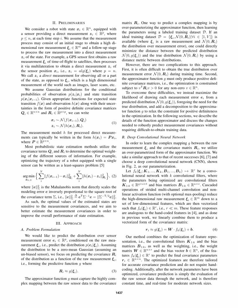
Fig. 3: Predicted covariance ellipses (red) and ground-truth

covariance ellipses (green) are shown for a few samples in

the simulated map. It can be seen that the Kullback-Leibler

divergence is quickly reduced in just 25 epochs.

IV. SIMULATION RESULTS

A. Simulation Setup

To validate our approach, we first picked a virtual en-

vironment where we could simulate a sensor with known

measurement covariances. Ground-truth covariances are nor-

mally difficult to obtain, but using a simulation environment

circumvented this difficulty. We picked a simulated position

sensor whose performance is correlated with the brightness

of the location xi ∈ R2 within a 2D map m ∈ R

k×k, i.e.,

Ri = f(xi,m). (14)

We designed the ground-truth sensor noise model f , con-

sisting of exponential and cosine functions, to introduce

complex non-linear noise characteristics. We then randomly

sampled 1000 locations xi within a known map m and for

each sample, computed the measurement covariance Ri from

which to draw an error label ei, i.e.,

ei ∼ N (xi, f(xi,m)). (15)

We chose the local region of the map m around the robot

position xi to be the raw measurement ξi, i.e.

ξi = h(xi,m), (16)

and obtained the training set D = {Ri, ei, ξi|∀i ∈ [1, V ]}.B. Simulation Results

We optimized the objective function g in Eq. 13 using

Stochastic Gradient Descent. Due to the simplicity of this

problem, we were able to reduce the complexity of the

function, removing convolution and reducing the network

size. After optimizing for 25 epochs, we obtained predicted

covariances g(ξi) for each raw measurement ξi. With access

to ground-truth covariance labels Ri, we evaluated the

Kullback-Leibler divergence (KLD) in Eq. 5 at each epoch.

As shown in Fig. 3, minimizing the negative log-likelihood

quickly reduced KLD, an evidence of the alternative opti-

mization in Eq. 6 reducing the direct distance metric. We

also compared a few representative covariance predictions

against the ground-truth for qualitative evaluation.

V. EXPERIMENT RESULTS

A. Experiment Setup

We evaluated the performance of DICE on predicting

the measurement covariances of the output of a 2D visual

odometry (VO) algorithm based on DVO [8]. The algorithm

densely aligns each RGB image to the previous image by

projecting the image into the world using known depth

information, then solving for the best back-projection into the

previous image that minimizes the photometric error between

the two. The difference between our 2D VO algorithm

and standard DVO is that back-projection is limited to 2D

motions, and no motion prior is used.

We chose the Microsoft Kinect as the raw measurement

sensor to pair with the algorithm, creating a Kinect-DVO

sensor that measures relative 2D motion. Based on the fact

that the odometry is computed by minimizing a metric in the

image-space (while the depth information is only used for

projections) and the similarity of consecutive RGB images

under moderate motion, we assumed that most predictive

features of uncertainty are in the latest RGB image. We

therefore chose only the latest RGB image as the input to

our predictor function g, although the VO algorithm required

both RGB images and a depth image to solve the alignment.

B. Training Data Collection

To generate training data, we collected RGB-D images

in an environment equipped with a Vicon motion capture

system. We obtained relative pose measurements using the

Kinect-DVO sensor, and computed the error in the mea-

surements as deviation from the Vicon measurements. We

collected approximately 42,500 pairs of images and error

labels as training data. In this experiment, we specifically

explored two common failure modes of VO algorithms: low

texture scenes and dynamic scenes. The environment was

set up to include varying degrees of texture, and a person

periodically walked in and out of the sensor frame during

data collection. The objects in the environments were also

moved around to prevent overfitting to the environment.

C. Network Structure and Training

While representing the covariance predictor as a CNN

removes the need to carefully specify a parametric form

of the covariance approximation function, high-level design

choices (width, depth, etc) are required for the network.

We used an eight layer deep CNN and the input RGB

images were down-sampled to 48x64 pixel greyscale images.

Each of the two convolutional layers consisted of 32 kernels

of size 5x5, followed by a 2x2 max pooling layer. Before

the output, there was one fully connected layer of 256 units,

and a dropout layer with a dropout rate of 50% to prevent

overfitting. The network, visualized in Fig. 2, was trained

using an Nvidia GeForce GTX 1080 for 6000 epochs, with

a learning rate of 0.0001, a Nesterov momentum of 0.9, and

a mini-batch size of 500. After experimenting with different

nonlinear activation functions, we found that a leaky rectify

activation [9] provided the most stable optimization.

1439

−1.0 −0.5 0.0 0.5 1.0

−0.5

0.0

0.5

1.0

1.5

2.0

2.5

012

3

4

5

0 1

2 3

4 5

−1.0 −0.5 0.0 0.5 1.0

−1.5

−1.0

−0.5

0.0

0.5

1.0

1.5

2.0

0

1

2

3

4

5

0 1

2 3

4 5

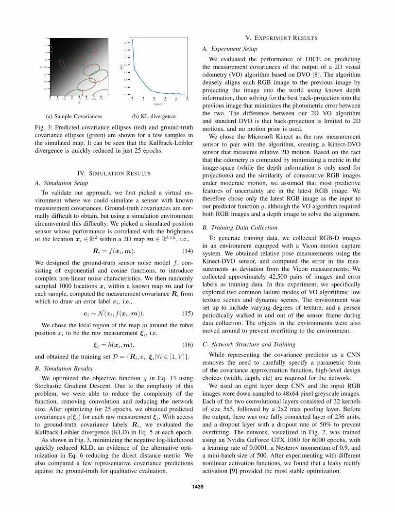
Fig. 4: Constant (blue) and DICE (red) measurement covariances are plotted for the Dynamic (left) and Unseen-Dynamic(right) datasets. The thumbnail images show the RGB frames at the correspondingly labeled points on the ground-truth

trajectories (black). The constant covariance, which is empirically fit to the training data and non-spherical, underestimates

the error in non-static scenes (i.e., 1 and 2 in Dynamic, 2 and 5 in Unseen-Dynamic) and overestimates in static scenes.

DICE covariances vary largely both in magnitude and shape (larger and elongated in non-static scenes, while small and

spherical in static scenes), more accurately representing the distribution of measurement error in different scenes. The major

and minor axes of the covariance were enlarged by a factor of 20 for visualization purposes.

D. Test Sets

We chose four test sets to benchmark DICE:

• Dynamic: A person present in the training dataset

walked across the camera frame once

• White-wall: The Kinect moved in a loop with two

separate low texture scenes

• Unseen-Dynamic: A person not present in the training

dataset walked across the camera frame twice

• TUM: This is the freiburg3 walking static dataset (from

the TUM [10] RGB-D SLAM benchmarks). The Kinect

was static and two people walked in and out of frame

The first three, Dynamic, White-wall and Unseen-Dynamic,

were drawn from the environments in the training data.

For reporting the likelihood metric, we removed data points

where Vicon measurements were measurably wrong (approx-

imately 2% of the measurements).

E. Measurement Likelihood Performance

In real environments, we do not have access to the true

distribution over measurement error to compare directly

against the predicted distributions as done in Section IV.

Instead, we could compare the likelihood of drawing true

measurement errors from predicted distributions as in Eq. 6.

We benchmarked the covariance prediction performance

of DICE against a constant covariance model, DVO’s in-

ternal prediction based on the Cramer-Rao bound [11], and

CELLO. To determine an appropriate constant covariance,

we calculated a single covariance over all of the training data.

The Cramer-Rao covariances were obtained by inverting

the Fisher information matrices of the dense photometric

alignment and multiplying by an empirically-determined

factor to compensate for the bounds being lower-bounds and

largely conservative. We used the empirical factor provided

TABLE I: Mean log-likelihood results are shown for each

prediction method and dataset pair. Values marked with

† were generated after the prediction method was further

trained with the augmented training dataset. On average,

DICE predicted covariances better modeled the errors over

all four test sets, and each DICE covariance prediction took

approximately 0.01 seconds, in Python using a modern i7.

Dynamic White-wall Unseen-Dynamic TUMConstant 9.20 8.84 9.27 8.62

Cramer-Rao -26.72 -2.92 -29.06 4.95

CELLO 10.61 9.52 10.36 9.15†DICE 11.80 10.38 11.13 9.63†

in the open-source implementation of DVO, noting that this

parameter can also be tuned to perform arbitrarily well on

any given dataset. The CELLO covariances were obtained

using 10 image-space features proposed in [12] (e.g. dynamic

range, pixel entropy, image gradients, etc) and the entire

training dataset for DICE was used as potential neighbors

in the kernel estimator. A few representative constant and

DICE measurement covariances are shown in Fig. 4.

Table I summarizes the performance of the four methods

on each test set described in Section V-D. We observed that

on average, the covariances estimated by DICE better ex-

plained the observations than those of the other approaches.

Fig. 6 illustrates the predictive performance of DICE on

Dynamic test set; regions of the trajectory characterized

by larger measurement error magnitudes were paired with

larger covariance estimates by DICE. In comparison, the

constant covariance method was unable to adapt, the Cramer-

Rao approach was still a severe underestimate, and CELLO

adapted but underestimated the magnitude of the covariance.

To test how well our method generalizes to new scenar-

ios and environments, we considered the Unseen-Dynamic

1440

0 100 200 300 400 500 600 700

0.000

0.025

0.050

0.075Error

magnitude

0 100 200 300 400 500 600 700

Time index

0.0000

0.0005

0.0010

0.0015

Trace 0

1

2Constant

Cramer-Rao

CELLO

DICE

0 1 2

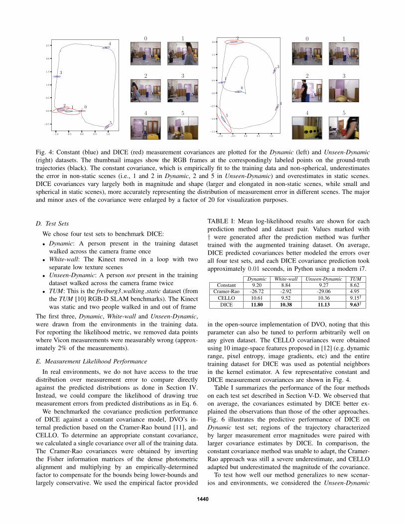
Fig. 5: The trace of the predicted measurement covariances

of all four methods on the TUM dataset are shown, with

representative images for small (1) and larger (0 and 2)

magnitude trace predictions. The grey shaded region indi-

cates the samples that were used to augment the existing

training dataset, while the unshaded portions were reserved

for testing. DICE outperforms the other three methods,

predicting larger covariances in regions of higher error.

dataset. Although this dataset was set in the same environ-

ment as was used to train DICE, the person in this test set was

not present in the training dataset. We observed that DICE

predicted more likely measurement models, on average, than

the other covariance prediction methods, indicating that the

low-level representation was general to some degree.

To test the adaptability of our approach, we considered the

TUM dataset, which has both an entirely new environment

and new people. We augmented the original training dataset

with the first 400 samples of the TUM dataset, and tuned

the pre-trained network with the augmented dataset (for

comparison purposes, we also augment the CELLO training

dataset). The average log-likelihood results over the entire

TUM dataset is reported in Table I. Fig. 5 illustrates that

given examples of a new environment, DICE can be re-

optimized to predict better measurement models than con-

stant, Cramer-Rao, and CELLO models, better distinguishing

the measurement error in static and dynamic scenes. This

example further illustrates a strength of data-driven feature

discovery, providing evidence that the predictions can be

further improved in new environments by taking pre-trained

models and resuming optimization on new data.

F. Trajectory Estimation Performance

We adapted the generic single-sensor trajectory optimiza-

tion in Eq. 2 to test the utility of accurately predicting

covariances of relative visual odometry measurements. Since

our VO measurements fully observe the robot state relative

to the previous state, the measurement model is simply

h(xi,xi−1) = xi − xi−1. We removed the state transition

model to best highlight the differences between covariance

prediction methods, and added a ground-truth loop-closure

0 200 400 600 800 1000

0.00

0.02

0.04

0.06

Error

magnitude

0 200 400 600 800 1000

Time index

0.000

0.001

0.002

0.003

Trace

Constant

Cramer-Rao

CELLO

DICE

Fig. 6: Raw measurement errors in Dynamic test set are

shown along with the trace of predicted covariances. The

trace of DICE covariance is highly correlated with the

error, demonstrating that DICE can accurately predict the

uncertainty of the measurements.

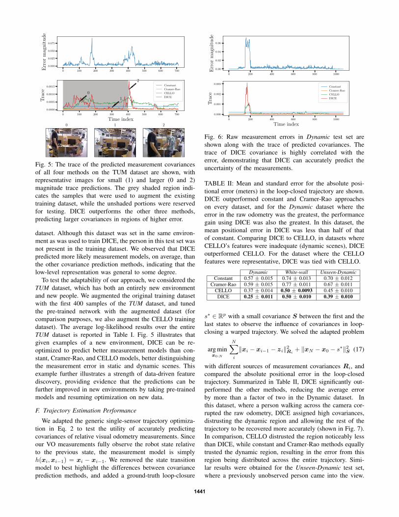
TABLE II: Mean and standard error for the absolute posi-

tional error (meters) in the loop-closed trajectory are shown.

DICE outperformed constant and Cramer-Rao approaches

on every dataset, and for the Dynamic dataset where the

error in the raw odometry was the greatest, the performance

gain using DICE was also the greatest. In this dataset, the

mean positional error in DICE was less than half of that

of constant. Comparing DICE to CELLO, in datasets where

CELLO’s features were inadequate (dynamic scenes), DICE

outperformed CELLO. For the dataset where the CELLO

features were representative, DICE was tied with CELLO.

Dynamic White-wall Unseen-DynamicConstant 0.57 ± 0.015 0.74 ± 0.013 0.70 ± 0.012

Cramer-Rao 0.59 ± 0.015 0.77 ± 0.011 0.67 ± 0.011CELLO 0.37 ± 0.014 0.50 ± 0.0093 0.45 ± 0.010DICE 0.25 ± 0.011 0.50 ± 0.010 0.39 ± 0.010

s∗ ∈ Rp with a small covariance S between the first and the

last states to observe the influence of covariances in loop-

closing a warped trajectory. We solved the adapted problem

arg minx0:N

N∑i

‖xi − xi−1 − zi‖2Ri+ ‖xN − x0 − s∗‖2S (17)

with different sources of measurement covariances Ri, and

compared the absolute positional error in the loop-closed

trajectory. Summarized in Table II, DICE significantly out-

performed the other methods, reducing the average error

by more than a factor of two in the Dynamic dataset. In

this dataset, where a person walking across the camera cor-

rupted the raw odometry, DICE assigned high covariances,

distrusting the dynamic region and allowing the rest of the

trajectory to be recovered more accurately (shown in Fig. 7).

In comparison, CELLO distrusted the region noticeably less

than DICE, while constant and Cramer-Rao methods equally

trusted the dynamic region, resulting in the error from this

region being distributed across the entire trajectory. Simi-

lar results were obtained for the Unseen-Dynamic test set,

where a previously unobserved person came into the view.

1441

−1 0 1 2

−1

0

1

2

3

−1 0 1 2

−1

0

1

2

3

−1 0 1 2

−1

0

1

2

3

−1 0 1 2

−1

0

1

2

3

−1 0 1 2

−1

0

1

2

3

Dyn

amic

−1 0 1 2 3

−1

0

1

2

3

−1 0 1 2 3

−1

0

1

2

3

−1 0 1 2 3

−1

0

1

2

3

−1 0 1 2 3

−1

0

1

2

3

−1 0 1 2 3

−1

0

1

2

3

Uns

een-

Dyn

amic

−3 −2 −1 0 1 2

−2

0

2

4

−3 −2 −1 0 1 2

−2

0

2

4

−3 −2 −1 0 1 2

−2

0

2

4

−3 −2 −1 0 1 2

−2

0

2

4

−3 −2 −1 0 1 2

−2

0

2

4

Whi

te-w

all

Ground-truth vicon trajectoryRaw trajectory (no loop closure)

Constant covariance optimized trajectoryCramer-Rao covariances optimized trajectory

CELLO covariances optimized trajectoryDICE optimized trajectory

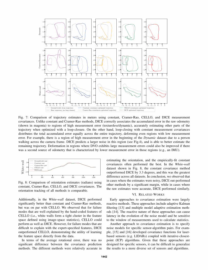
Fig. 7: Comparison of trajectory estimates in meters using constant, Cramer-Rao, CELLO, and DICE measurement

covariances. Unlike constant and Cramer-Rao methods, DICE correctly associates the accumulated error in the raw odometry

(shown in magenta) to regions of high measurement error (textureless/dynamic), accurately estimating other parts of the

trajectory when optimized with a loop-closure. On the other hand, loop-closing with constant measurement covariances

distributes the total accumulated error equally across the entire trajectory, deforming even regions with low measurement

error. For example, there is a region of high measurement error in the beginning of the Dynamic dataset due to a person

walking across the camera frame. DICE predicts a larger noise in this region (see Fig.4), and is able to better estimate the

remaining trajectory. Deformation in regions where DVO exhibits large measurement errors could also be improved if there

was a second source of odometry that is characterized by lower measurement error in those regions (e.g., an IMU).

0 200 400 600 800 1000 1200

−2

0

2

White-wall Groundtruth yaw

Constant yaw

Cramer-Rao yaw

CELLO yaw

DICE yaw

Fig. 8: Comparison of orientation estimates (radians) using

constant, Cramer-Rao, CELLO, and DICE covariances. The

orientation tracking of all methods is comparable.

Additionally, in the White-wall dataset, DICE performed

significantly better than constant and Cramer-Rao methods,

but was on par with CELLO. We observed that for failure

modes that are well explained by the hand-coded features of

CELLO (i.e., white walls form a tight cluster in the feature

space defined using image-space statistics), CELLO could

perform as well as DICE. However, for failure modes that are

difficult to explain with the expert-specified features, DICE

outperformed CELLO, demonstrating the utility of learning

the feature space directly from the data.

In terms of the average rotational error, there was no

significant difference between the covariance prediction

methods. The different methods were relatively accurate in

estimating the orientation, and the empirically-fit constant

covariances often performed the best. In the White-walldataset shown in Fig. 8, the constant covariance method

outperformed DICE by 3.3 degrees, and this was the greatest

difference across all datasets. In conclusion, we observed that

in cases where the estimates were noisy, DICE out-performed

other methods by a significant margin, while in cases where

the raw estimates were accurate, DICE performed similarly.

VI. RELATED WORKS

Early approaches to covariance estimation were largely

reactive methods. These approaches include adaptive Kalman

filtering [13] and multiple model adaptive estimation meth-

ods [14]. The reactive nature of these approaches can cause

latency in the evolution of the noise model and be sensitive

to the window of measurements used to calculate statistics.Another approach to covariance estimation is to specify

noise models for specific sensor-algorithm pairs. For exam-

ple, [15] and [16] developed covariance functions for laser-

based sensors (e.g. LIDARs) coupled with iterative-closest-

point (ICP) algorithms. Given that these approaches are

designed for specific sensors, it can be difficult to generalize

the results to a more diverse set of sensors and algorithms.

1442

There is a significant body of literature regarding non-

parametric approaches to predictive covariance estimation.

For example, Ko et. al. [17] described how to use Gaussian

Processes to estimate heteroscedastic Gaussian noise models,

and Tallavajhula et. al. [18] proposed generic non-parametric

noise models. However, these types of approaches also suffer

from scaling problems without a lower-dimensional feature

space. We note that feature specification is itself a topic of

research, as in [19], which experimentally designs expertly

hand-coded features for use in covariance estimation.

The neural network community has also previously esti-

mated arbitrary probability distributions for joint [20] and

conditional distributions [21], but proper backpropagation

proved to be computationally expensive. Williams described

how neural networks could be used to model conditional

multivariate densities [22], proposing special “dispersion”

nodes to learn the parameters of a Cholesky decomposition.

They demonstrate the approach on one and two dimensional

examples, and extend to time series financial data.

Recent work [23], [24] using neural networks to estimate

uncertainties adopt similar log-likelihood models to ours.

[23] assumes a diagonal covariance matrix and estimates

the mean as well as the covariance of a specific end-to-end

learned VO sensor. [24] combines heterodescedatic aleatoric

noise, which we model, with epistemic noise in a single

model, but is orders of magnitude slower due to the expensive

Monte Carlo sampling required for the epistemic noise.

VII. CONCLUSION

We have presented DICE – a novel method for predicting

measurement noise of complex sensors without using ex-

tensive domain knowledge. We demonstrated that DICE can

accurately predict the measurement covariance of a simulated

light sensor, and a visual odometry sensor. We have shown

that predicting accurate measurement covariances can help

improve trajectory estimates, and achieve accuracy signifi-

cantly better than conventional methods for difficult scenes.

ACKNOWLEDGMENT

This work was supported by NASA under Award No.

NNX15AQ50A and DARPA under Fast Lightweight Auton-

omy (FLA) program, Contract No. HR0011-15-C-0110.

REFERENCES

[1] J. Engel, T. Schops, and D. Cremers, “LSD-SLAM:

Large-scale direct monocular SLAM,” in ECCV 2014.

[2] K. Ok, W. N. Greene, and N. Roy, “Simultaneous

tracking and rendering: Real-time monocular localiza-

tion for MAVs,” in Proc. ICRA 2016.

[3] W. Vega-Brown, A. Bachrach, A. Bry, J. Kelly, and

N. Roy, “CELLO: A fast algorithm for covariance

estimation,” in Proc. ICRA 2013.

[4] H. Hu and G. Kantor, “Parametric covariance predic-

tion for heteroscedastic noise,” in Proc. IROS 2015.

[5] F. Dellaert and M. Kaess, “Square root sam: Si-

multaneous localization and mapping via square root

information smoothing,” IJRR, vol. 25, no. 12,

[6] Q. V. Le, “Building high-level features using large

scale unsupervised learning,” in Proc. ICASSP 2013.

[7] K. Simonyan and A. Zisserman, “Very deep convo-

lutional networks for large-scale image recognition,”

arXiv:1409.1556, 2014.

[8] C. Kerl, J. Sturm, and D. Cremers, “Robust odometry

estimation for RGB-D cameras,” in Proc. ICRA 2013.

[9] A. L. Maas, A. Y. Hannun, and A. Y. Ng, “Rectifier

nonlinearities improve neural network acoustic mod-

els,” in Proc. ICML, vol. 30, 2013.

[10] J. Sturm, N. Engelhard, F. Endres, W. Burgard, and

D. Cremers, “A benchmark for the evaluation of RGB-

D SLAM systems,” in Proc. IROS, 2012.

[11] C. R. Rao, “Information and the accuracy attainable in

the estimation of statistical parameters,” Bull. CalcuttaMath. Soc., vol. 37, pp. 81–89, 1945.

[12] W. Vega-Brown, “Predictive parameter estimation for

bayesian filtering,” Master’s thesis, Massachusetts In-

stitute of Technology, 2013.

[13] R. Mehra, “On the identification of variances and

adaptive Kalman filtering,” IEEE Transactions on Au-tomatic Control, vol. 15, no. 2, pp. 175–184, 1970.

[14] D Magill, “Optimal adaptive estimation of sampled

stochastic processes,” IEEE Transactions on Auto-matic Control, vol. 10, no. 4, pp. 434–439, 1965.

[15] A. Censi, “An accurate closed-form estimate of ICP’s

covariance,” in Proc. ICRA 2007.

[16] M. Barczyk and S. Bonnabel, “Towards realistic co-

variance estimation of ICP-based Kinect V1 scan

matching: The 1D case,” in Proc. ACC 2017.

[17] J. Ko and D. Fox, “GP-BayesFilters: Bayesian filtering

using Gaussian process prediction and observation

models,” Autonomous Robots, vol. 27, no. 1,

[18] A. Tallavajhula, B. Poczos, and A. Kelly, “Non-

parametric distribution regression applied to sensor

modeling,” in Proc. IROS 2016.

[19] V. Peretroukhin, L. Clement, M. Giamou, and J. Kelly,

“PROBE: Predictive robust estimation for visual-

inertial navigation,” in Proc. IROS 2015.

[20] D. S. Modha and Y. Fainman, “A learning law for

density estimation,” IEEE Transactions on NeuralNetworks, vol. 5, no. 3, pp. 519–523, 1994.

[21] A. Sarajedini, R. Hecht-Nielsen, and P. M. Chau,

“Conditional probability density function estimation

with sigmoidal neural networks,” IEEE Transactionson neural networks, vol. 10, no. 2, pp. 231–238, 1999.

[22] P. M. Williams, “Using neural networks to model con-

ditional multivariate densities,” Neural Computation,

vol. 8, no. 4, pp. 843–854, 1996.

[23] S. Wang, R. Clark, H. Wen, and N. Trigoni,

“End-to-end, sequence-to-sequence probabilistic vi-

sual odometry through deep neural networks,” IJRR,

p. 0 278 364 917 734 298, 2017.

[24] A. Kendall and Y. Gal, “What uncertainties do we

need in bayesian deep learning for computer vision?”

In Proc. NIPS, 2017.

1443