Embed Size (px)
Citation preview

Coupling and Simulation of Acoustic Fluid-Structure
Interaction Systems Using Localized Lagrange Multipliers
by
Mike R. Ross
B.S., Colorado School of Mines, 1998
M.S., University of Colorado, Boulder, 2004
A thesis submitted to the
Faculty of the Graduate School of the
University of Colorado in partial fulfillment
of the requirements for the degree of
Doctor of Philosophy
Department of Aerospace Engineering Science
2006

This thesis entitled:Coupling and Simulation of Acoustic Fluid-Structure Interaction Systems Using Localized Lagrange
Multiplierswritten by Mike R. Ross
has been approved for the Department of Aerospace Engineering Science
Carlos Felippa
K.C. Park
Date
The final copy of this thesis has been examined by the signatories, and we find that both the contentand the form meet acceptable presentation standards of scholarly work in the above mentioned
discipline.

iii
Ross, Mike R. (Ph.D., Aerospace Engineering Science)
Coupling and Simulation of Acoustic Fluid-Structure Interaction Systems Using Localized Lagrange
Multipliers
Thesis directed by Prof. Carlos Felippa
This thesis presents a new coupling method for treating the interaction of an acoustic fluid with
a flexible structure, with emphasis on handling spatially non-matching meshes. It is based on the
Localized Lagrange Multiplier (LLM) method. A frame is introduced as a ”mediator” or ”information
relay” device between the fluid and the structure at the interaction surface. The frame is discretized
in terms of kinematic variables. A Lagrange multiplier field is introduced between the frame and the
structure, and another one between the frame and the fluid. The function of the multiplier pair is
weak enforcement of kinematic continuity. This configuration completely decouples the structure and
fluid models, because each model communicates to the frame through node collocated multipliers and
not directly to each other.
In order to assure proper communication, energy formulations of the fluid and structure models
are in terms of displacements and associated time derivatives. A novel transformation of the fluid
displacement model into a fluid displacement potential model enforces the irrotational condition of
the acoustic fluid. This transformation reduces the number of degrees of freedom in two and three-
dimensions and is suitable for both vibration and transient analyses.
The LLM method facilitates the construction of separate discretizations using different mesh gen-
eration programs, as well as use of customized time integration methods. To advance the solution in
time, the LLM coupling method is combined with a partitioned solution procedure. The time-stepping
computations are organized in a way that eliminates the traditional prediction step characteristic of
staggered solution procedures. This is accomplished by solving for the interface variables: Lagrange
multipliers and frame states, and then feeding this solution back to the coupled components. This
sequence forestalls the well-known stability degradation caused by prediction, yet it retains the de-
sirable localization features of a partitioned analysis procedure. One consequence of this method is
that if two A-stable integration schemes, such as the trapezoidal rule, are chosen for the fluid and
structure, then the coupled system retains unconditional stability. Other time integration schemes,
such as central difference, for one or both components can be readily accommodated.
iv
Acknowledgements
Above all, I would like to thank my advisor, Prof. Carlos Felippa, for his patience and his
guidance. I express my thanks to my committee members: Prof. K.C. Park, Prof. Thomas Geers,
Prof. Kurt Maute, Prof. Stein Sture, and Prof. Michael Sprague, for their insight and amazing patience
with my constant interruptions. I am grateful to the Center for Aerospace Structures, particularly
Deborah Mellblom and my fellow graduate students for their assistances and entertainment. Special
thanks is given to Dr. Hiraku Sakamoto for his support with the vibration analysis, and to Christophe
Kassiotis for his assistances with the Bleich-Sandler plate problem. Finally, I thank all those intrepid
souls that went climbing with me and helped maintain my sanity. This research was funded by NSF
grant CMS 0219422.
Of course, I am deeply indebted to my wife for all her support, and willingness to put her dreams
on hold.

v
Contents
Chapter
1 Introduction 1
1.1 Thesis Overview . . . . . . . . . . . . . . . . . . . . . . . . . . . . . . . . . . . . . . . 2
1.2 Main Thesis Contributions . . . . . . . . . . . . . . . . . . . . . . . . . . . . . . . . . . 6
1.3 Manuscript Organization . . . . . . . . . . . . . . . . . . . . . . . . . . . . . . . . . . . 7
2 Localized Lagrange Multiplier Method for Acoustic FSI 9
2.1 Introduction . . . . . . . . . . . . . . . . . . . . . . . . . . . . . . . . . . . . . . . . . . 9
2.2 System’s Energy Functionals . . . . . . . . . . . . . . . . . . . . . . . . . . . . . . . . 11
2.3 Finite Element Implementation . . . . . . . . . . . . . . . . . . . . . . . . . . . . . . . 14
2.3.1 Discretization of the Partitioned Domains . . . . . . . . . . . . . . . . . . . . . 14
2.3.2 Lagrange Multiplier Boundary Discretization . . . . . . . . . . . . . . . . . . . 15
2.3.3 Interface Frame Discretization . . . . . . . . . . . . . . . . . . . . . . . . . . . 17
2.3.4 Lagrange Multiplier Shape Functions Revisited . . . . . . . . . . . . . . . . . . 22
2.3.5 Matrix Form of the Total System Functional . . . . . . . . . . . . . . . . . . . 23
2.4 Inclusion of Irrotational Assumption by the Displacement Potential . . . . . . . . . . . 25
2.4.1 Circulation Modes . . . . . . . . . . . . . . . . . . . . . . . . . . . . . . . . . . 25
2.4.2 Gradient Matrix . . . . . . . . . . . . . . . . . . . . . . . . . . . . . . . . . . . 26
2.5 The Variation of the Energy Functional . . . . . . . . . . . . . . . . . . . . . . . . . . 30
2.6 Summary . . . . . . . . . . . . . . . . . . . . . . . . . . . . . . . . . . . . . . . . . . . 31
3 Transient Concepts Using Localized Lagrange Multipliers 32
3.1 Introduction . . . . . . . . . . . . . . . . . . . . . . . . . . . . . . . . . . . . . . . . . . 32
3.2 Partitioned Transient Analysis . . . . . . . . . . . . . . . . . . . . . . . . . . . . . . . 33
3.2.1 Scaling the Interface Equation . . . . . . . . . . . . . . . . . . . . . . . . . . . 36
3.3 Inclusion of Concept for other FSI Methods (i.e. CASE) . . . . . . . . . . . . . . . . . 39

vi
3.3.1 Relation Between Fluid Pressure and Structure Force . . . . . . . . . . . . . . 39
3.3.2 Relation between Subsystems’ Boundary Displacements . . . . . . . . . . . . . 41
3.4 Error/ Accuracy . . . . . . . . . . . . . . . . . . . . . . . . . . . . . . . . . . . . . . . 42
3.4.1 Geer’s C-Error Method . . . . . . . . . . . . . . . . . . . . . . . . . . . . . . . 44
3.4.2 Energy Error . . . . . . . . . . . . . . . . . . . . . . . . . . . . . . . . . . . . . 44
3.5 Summary . . . . . . . . . . . . . . . . . . . . . . . . . . . . . . . . . . . . . . . . . . . 46
4 Validation of Fluid Code: Pressure on Dam Face 47
4.1 Introduction . . . . . . . . . . . . . . . . . . . . . . . . . . . . . . . . . . . . . . . . . . 47
4.2 Problem Description and Analytical Solution . . . . . . . . . . . . . . . . . . . . . . . 47
4.3 Fluid Code Validation . . . . . . . . . . . . . . . . . . . . . . . . . . . . . . . . . . . . 49
4.4 Incorporation of Silent Boundaries . . . . . . . . . . . . . . . . . . . . . . . . . . . . . 51
4.5 Silent Boundary Validation . . . . . . . . . . . . . . . . . . . . . . . . . . . . . . . . . 56
4.6 Inclusion of Surface Waves . . . . . . . . . . . . . . . . . . . . . . . . . . . . . . . . . . 57
4.7 Summary . . . . . . . . . . . . . . . . . . . . . . . . . . . . . . . . . . . . . . . . . . . 59
5 Validation of Concept: Infinite Piston Problem 61
5.1 Introduction . . . . . . . . . . . . . . . . . . . . . . . . . . . . . . . . . . . . . . . . . . 61
5.2 Problem Description . . . . . . . . . . . . . . . . . . . . . . . . . . . . . . . . . . . . . 62
5.3 Analytical Model for 1-D Problem . . . . . . . . . . . . . . . . . . . . . . . . . . . . . 62
5.4 Current Computational Models . . . . . . . . . . . . . . . . . . . . . . . . . . . . . . . 65
5.5 LLM Method Results in 3-D . . . . . . . . . . . . . . . . . . . . . . . . . . . . . . . . . 67
5.5.1 Matching Meshes Results . . . . . . . . . . . . . . . . . . . . . . . . . . . . . . 67
5.5.2 Non-matching Results . . . . . . . . . . . . . . . . . . . . . . . . . . . . . . . . 67
5.5.3 Stability Verification . . . . . . . . . . . . . . . . . . . . . . . . . . . . . . . . . 71
5.6 Summary . . . . . . . . . . . . . . . . . . . . . . . . . . . . . . . . . . . . . . . . . . . 71
6 Gravity Dam Benchmark Study: Vibration Analysis 73
6.1 Problem Description . . . . . . . . . . . . . . . . . . . . . . . . . . . . . . . . . . . . . 73
6.2 Linear Vibration Analysis . . . . . . . . . . . . . . . . . . . . . . . . . . . . . . . . . . 74
6.2.1 Modal Analysis . . . . . . . . . . . . . . . . . . . . . . . . . . . . . . . . . . . . 74
6.2.2 Kinematic Continuity Issues . . . . . . . . . . . . . . . . . . . . . . . . . . . . . 77
6.2.3 Frequency Content of Acceleration . . . . . . . . . . . . . . . . . . . . . . . . . 81
6.2.4 Frequency Response Function . . . . . . . . . . . . . . . . . . . . . . . . . . . . 81

vii
6.3 Examples of Passing the Patch Test . . . . . . . . . . . . . . . . . . . . . . . . . . . . 83
6.4 Summary . . . . . . . . . . . . . . . . . . . . . . . . . . . . . . . . . . . . . . . . . . . 85
7 Gravity Dam Benchmark Study: Transient Analysis, and Error 87
7.1 Introduction . . . . . . . . . . . . . . . . . . . . . . . . . . . . . . . . . . . . . . . . . . 87
7.2 Load Vector . . . . . . . . . . . . . . . . . . . . . . . . . . . . . . . . . . . . . . . . . . 87
7.2.1 Relative Displacement’s Load Vector . . . . . . . . . . . . . . . . . . . . . . . . 88
7.2.2 Total Displacement’s Load Vector . . . . . . . . . . . . . . . . . . . . . . . . . 89
7.3 Matching Mesh Comparison for CASE/CAFE and LLM . . . . . . . . . . . . . . . . . 90
7.4 Scaling the Interface Matrix Verification . . . . . . . . . . . . . . . . . . . . . . . . . . 90
7.5 Non-Matching Mesh Comparisons for both CASE and LLM . . . . . . . . . . . . . . . 93
7.6 Summary . . . . . . . . . . . . . . . . . . . . . . . . . . . . . . . . . . . . . . . . . . . 98
8 Reduced Order Modeling and Cavitation with the Transient LLM method 99
8.1 Reduced Order Modeling . . . . . . . . . . . . . . . . . . . . . . . . . . . . . . . . . . 99
8.1.1 Computational Results for ROM . . . . . . . . . . . . . . . . . . . . . . . . . . 100
8.2 Cavitation . . . . . . . . . . . . . . . . . . . . . . . . . . . . . . . . . . . . . . . . . . . 101
8.2.1 Modification of the Fluid Element Stiffness for Cavitation . . . . . . . . . . . . 104
8.2.2 Frothing: Spurious Oscillations . . . . . . . . . . . . . . . . . . . . . . . . . . . 106
8.2.3 Bleich-Sandler Plate Problem . . . . . . . . . . . . . . . . . . . . . . . . . . . . 107
8.2.4 Cavitation in Koyna Dam Analysis . . . . . . . . . . . . . . . . . . . . . . . . . 109
8.3 Operational Count . . . . . . . . . . . . . . . . . . . . . . . . . . . . . . . . . . . . . . 114
8.4 Summary . . . . . . . . . . . . . . . . . . . . . . . . . . . . . . . . . . . . . . . . . . . 115
9 Partitioned 3-D Problem with Curved Surface 116
9.1 Problem Description . . . . . . . . . . . . . . . . . . . . . . . . . . . . . . . . . . . . . 116
9.2 Creation of the Connection Matrices . . . . . . . . . . . . . . . . . . . . . . . . . . . . 118
9.3 Non-matching Mesh Results . . . . . . . . . . . . . . . . . . . . . . . . . . . . . . . . . 122
9.4 Summary . . . . . . . . . . . . . . . . . . . . . . . . . . . . . . . . . . . . . . . . . . . 124
10 Conclusion 125
10.1 Future Work . . . . . . . . . . . . . . . . . . . . . . . . . . . . . . . . . . . . . . . . . 127

viii
Bibliography 128
Appendix
A CASE/CAFE Method 137
A.1 Fluid Equations . . . . . . . . . . . . . . . . . . . . . . . . . . . . . . . . . . . . . . . . 137
A.1.1 Fluid Governing Equations . . . . . . . . . . . . . . . . . . . . . . . . . . . . . 137
A.1.2 Spectral Elements . . . . . . . . . . . . . . . . . . . . . . . . . . . . . . . . . . 139
A.1.3 Silent Boundary of the Fluid . . . . . . . . . . . . . . . . . . . . . . . . . . . . 141
A.1.4 Explicit Time Integration . . . . . . . . . . . . . . . . . . . . . . . . . . . . . . 141
A.1.5 Stability of Fluid Time Integration . . . . . . . . . . . . . . . . . . . . . . . . . 142
A.2 Structure, Fluid, and the Silent Boundary Coupling . . . . . . . . . . . . . . . . . . . 142
A.3 Staggered Integration . . . . . . . . . . . . . . . . . . . . . . . . . . . . . . . . . . . . 143
B Mortar Method and the Consistent Interpolation Based Method 144
B.1 Mortar Method . . . . . . . . . . . . . . . . . . . . . . . . . . . . . . . . . . . . . . . . 144
B.2 Consistent Method . . . . . . . . . . . . . . . . . . . . . . . . . . . . . . . . . . . . . . 146
B.3 Relationship between LLM, Mortar, and Consistent Interpolation . . . . . . . . . . . . 147
C Discretization Error Bound for Linear Interpolation of the Field Variables at the Interface in
the LLM Method 149

ix
Tables
Table
3.1 Properties of well-known members of the Newmark method . . . . . . . . . . . . . . . 33
4.1 Parameters for the pressure on the dam face problem. . . . . . . . . . . . . . . . . . . 49
5.1 Parameters for the infinite piston fluid-structure system. . . . . . . . . . . . . . . . . . 62
6.1 Parameters for Koyna dam model. . . . . . . . . . . . . . . . . . . . . . . . . . . . . . 76
8.1 Parameters for the Bleich-Sandler plate problem . . . . . . . . . . . . . . . . . . . . . 109
9.1 Parameters for Morrow Point dam model. . . . . . . . . . . . . . . . . . . . . . . . . . 119

x
Figures
Figure
2.1 LLM Concept: (a)Given a system. (b) Divide the system into subdomains. (c) Insert
an interface displacement frame that is linked by the Local Lagrange Multipliers. . . . 10
2.2 Comparison of the LLM method to the Mortar method. (a) Localized Lagrange multi-
pliers. (b) Classical Lagrange multiplier. . . . . . . . . . . . . . . . . . . . . . . . . . . 15
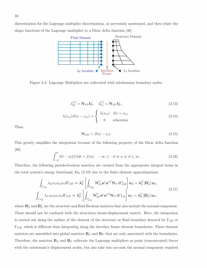
2.3 Lagrange Multipliers are collocated with subdomains boundary nodes. . . . . . . . . . 16
2.4 Graphical representation of the determination of the interface nodes in 2-D. . . . . . . 20
2.5 Integration over the straight line piece γi. . . . . . . . . . . . . . . . . . . . . . . . . . 24
2.6 Bilinear quadrilateral element . . . . . . . . . . . . . . . . . . . . . . . . . . . . . . . . 27
2.7 Two connected bilinear quadrilateral elements . . . . . . . . . . . . . . . . . . . . . . . 29
3.1 Graphical representation of the time stepping procedure for the LLM method. . . . . . 35
4.1 Rigid dam problem for fluid code verification. . . . . . . . . . . . . . . . . . . . . . . . 48
4.2 Analytical pressure on the rigid dam. . . . . . . . . . . . . . . . . . . . . . . . . . . . . 50
4.3 Fluid mesh with a characteristic length of 20 m. . . . . . . . . . . . . . . . . . . . . . 50
4.4 Pressure on dam face with a fluid characteristic length of 20 m. . . . . . . . . . . . . . 51
4.5 Pressure on dam face with a fluid characteristic length of 10 m. . . . . . . . . . . . . . 52
4.6 Pressure on dam face with a fluid characteristic length of 5 m. . . . . . . . . . . . . . 52
4.7 Viscous Damping Boundary concept [55]. . . . . . . . . . . . . . . . . . . . . . . . . . 55
4.8 Pressure on dam face with a fluid characteristic length of 10 m with and without a
silent boundary. . . . . . . . . . . . . . . . . . . . . . . . . . . . . . . . . . . . . . . . . 56
4.9 Pressure on dam face with a fluid characteristic length of 5 m with damping added to
the fluid. . . . . . . . . . . . . . . . . . . . . . . . . . . . . . . . . . . . . . . . . . . . . 57
4.10 Pressure on dam face with a fluid characteristic length of 5 m with damping added to
the fluid. . . . . . . . . . . . . . . . . . . . . . . . . . . . . . . . . . . . . . . . . . . . . 58

xi
4.11 Free surface wave . . . . . . . . . . . . . . . . . . . . . . . . . . . . . . . . . . . . . . . 59
5.1 Infinite piston fluid-structure system. . . . . . . . . . . . . . . . . . . . . . . . . . . . . 62
5.2 Free body diagram of a mass-spring system with water. . . . . . . . . . . . . . . . . . 63
5.3 Displacement of the mass in the infinite piston fluid-structure system by an analytical
method. . . . . . . . . . . . . . . . . . . . . . . . . . . . . . . . . . . . . . . . . . . . . 66
5.4 Displacement of the mass in the infinite piston fluid-structure system by existing com-
putational models. . . . . . . . . . . . . . . . . . . . . . . . . . . . . . . . . . . . . . . 67
5.5 Model with 3-D elements for the LLM method. . . . . . . . . . . . . . . . . . . . . . . 68
5.6 Comparison between analytical and LLM method with no visible error; C-error = 0.0007. 68
5.7 Model with non-matching meshes. . . . . . . . . . . . . . . . . . . . . . . . . . . . . . 69
5.8 Interface frame for the non-matching mesh. . . . . . . . . . . . . . . . . . . . . . . . . 70
5.9 C-error for the infinite piston system with non-matching meshes. . . . . . . . . . . . . 70
5.10 Time step values and the error associated with the time steps. . . . . . . . . . . . . . 71
6.1 Downstream views of the Koyna dam: (a)Present day. (b) After the earthquake of
Decemeber 1967. . . . . . . . . . . . . . . . . . . . . . . . . . . . . . . . . . . . . . . . 74
6.2 Koyna dam-reservoir system. . . . . . . . . . . . . . . . . . . . . . . . . . . . . . . . . 75
6.3 El Centro earthquake May 18, 1940, horizontal component. . . . . . . . . . . . . . . . 75
6.4 Koyna dam-reservoir system with non-matching meshes . . . . . . . . . . . . . . . . . 78
6.5 Mode frequencies and mode shapes of the system . . . . . . . . . . . . . . . . . . . . . 79
6.6 5th Mode shape of the system for the Mortar method with the interface discretized as
the coarse mesh. . . . . . . . . . . . . . . . . . . . . . . . . . . . . . . . . . . . . . . . 80
6.7 30th Mode shape of the system for the LLM method with the interface discretized as
the refined mesh. . . . . . . . . . . . . . . . . . . . . . . . . . . . . . . . . . . . . . . . 80
6.8 Frequency content of the seismic acceleration. . . . . . . . . . . . . . . . . . . . . . . . 81
6.9 Frequency response of the partitioned subsystems. . . . . . . . . . . . . . . . . . . . . 82
6.10 Frequency response of the assembled system. . . . . . . . . . . . . . . . . . . . . . . . 83
6.11 Frequency response of the assembled system with the dam face as the output DOF. . 84
6.12 Frequency response of the assembled system with the dam Lagrange multiplier as the
input DOF. . . . . . . . . . . . . . . . . . . . . . . . . . . . . . . . . . . . . . . . . . . 84
6.13 An example of a constant state of stress across the interface frame. . . . . . . . . . . . 84
6.14 An example of a constant state of stress across the interface frame, where ”x” is the
locations of the interface nodes. . . . . . . . . . . . . . . . . . . . . . . . . . . . . . . . 86

xii
7.1 Relative displacement concept. . . . . . . . . . . . . . . . . . . . . . . . . . . . . . . . 88
7.2 Total displacement concept. . . . . . . . . . . . . . . . . . . . . . . . . . . . . . . . . . 89
7.3 Portion of Koyna dam mesh used as benchmark mesh for C-error. . . . . . . . . . . . 91
7.4 C-error values with matching meshes. . . . . . . . . . . . . . . . . . . . . . . . . . . . 91
7.5 Crest Displacement of Koyna dam of converge results for the transient analysis by the
LLM method and the CASE method. . . . . . . . . . . . . . . . . . . . . . . . . . . . 91
7.6 Energy difference caused by scaling at the interface of matching meshes. Energy on one
side of the interface is of the magnitude of 106 Nm on average. . . . . . . . . . . . . . 92
7.7 Dam crest displacement values for different interface meshing with LLM for the transient
analysis and non-matching meshes. . . . . . . . . . . . . . . . . . . . . . . . . . . . . . 93
7.8 Transfer of forces with the LLM method. . . . . . . . . . . . . . . . . . . . . . . . . . 94
7.9 Energy difference across the interface frame. Average energy on structure side is
6.78x10⁶Nm. . . . . . . . . . . . . . . . . . . . . . . . . . . . . . . . . . . . . . . . . . 95
7.10 Dam crest displacement values for different interface meshing with CASE for the tran-
sient analysis and LLM for the non-matching meshes. . . . . . . . . . . . . . . . . . . 95
7.11 Dam crest displacement values for different interface meshing with CASE for the tran-
sient analysis and Mortar for the non-matching meshes. . . . . . . . . . . . . . . . . . 96
7.12 C-error for different Total DOF of non-matching meshes. . . . . . . . . . . . . . . . . . 97
8.1 Characteristic portion of the non-matching mesh used for the ROM test. . . . . . . . . 101
8.2 Reduction of system up to the frequency of the eigenvector. . . . . . . . . . . . . . . . 102
8.3 Dam crest displacement values for a reduced order model using 20% of the eigenvectors
of the structure and the fluid. . . . . . . . . . . . . . . . . . . . . . . . . . . . . . . . . 102
8.4 Density pressure relation for a bilinear fluid [114]. . . . . . . . . . . . . . . . . . . . . . 103
8.5 Schematic model of the Bleich-Sandler plate problem. . . . . . . . . . . . . . . . . . . 108
8.6 Bleich-Sandler plate problem results . . . . . . . . . . . . . . . . . . . . . . . . . . . . 110
8.7 Koyna dam mesh used for cavitation analysis. . . . . . . . . . . . . . . . . . . . . . . . 110
8.8 The effects of cavitation on the relative displacement of the dam crest. . . . . . . . . . 110
8.9 Cavitation zone during selective time intervals with the Dam’s face on the right side. . 111
8.10 Cavitation zone during selective time intervals with the Dam’s face on the right side
without suppressing frothing. . . . . . . . . . . . . . . . . . . . . . . . . . . . . . . . . 111
8.11 The effects of cavitation on the relative displacement of the dam crest with the maximum
acceleration equal to 1.5g. . . . . . . . . . . . . . . . . . . . . . . . . . . . . . . . . . . 112

xiii
8.12 The effects of cavitation on the relative displacement of the dam crest with the maximum
acceleration equal to 1.5g, but with the acceleration in the opposite direction than
previously. . . . . . . . . . . . . . . . . . . . . . . . . . . . . . . . . . . . . . . . . . . . 113
9.1 Morrow Point dam representation. . . . . . . . . . . . . . . . . . . . . . . . . . . . . . 117
9.2 Ground motion and frequency content of the seismic acceleration recorded at the 1952
Taft Lincoln School Tunnel, California earthquake. . . . . . . . . . . . . . . . . . . . . 118
9.3 Morrow Point dam model used for this study. The fluid is not shown and the foundation,
shown in brown, is rigid. . . . . . . . . . . . . . . . . . . . . . . . . . . . . . . . . . . . 119
9.4 Mapping of the subdomains nodes to an interface element for use in the zero-moment
rule. . . . . . . . . . . . . . . . . . . . . . . . . . . . . . . . . . . . . . . . . . . . . . . 120
9.5 Interface nodes ”x” determined by the zero-moment rule. . . . . . . . . . . . . . . . . 121
9.6 Structure Mesh that showed Convergence. . . . . . . . . . . . . . . . . . . . . . . . . . 123
9.7 Relative displacement comparison for non-matching mesh versus matched mesh with
63 structure interface nodes. . . . . . . . . . . . . . . . . . . . . . . . . . . . . . . . . . 123
9.8 The effects of cavitation on the relative displacement of the dam crest with the maximum
acceleration equal to 1 g. . . . . . . . . . . . . . . . . . . . . . . . . . . . . . . . . . . 124
B.1 An example of how the LLM method, the Mortar method, and the Consistent Interpo-
lation method can produce the same relation matrices. . . . . . . . . . . . . . . . . . . 148
C.1 Discretization error for the portion of the constraint functional∫
ΓiλF i(uF i − uBi)dΓi . 150

Chapter 1
Introduction
The dynamic interaction between a fluid and a structure is a significant concern in many engi-
neering problems. These problems include systems as diverse as offshore and submerged structures,
storage tanks, biomechanical systems, inkjet printers, aircrafts, and suspension bridges. The interac-
tion can drastically change the dynamic characteristics of the structure and consequently its response
to transient, cyclic, and stochastic excitation. Therefore, it is desired to accurately model these diverse
systems with the inclusion of the fluid-structure interaction (FSI).
In the FSI problem, the fluid behavior can vary greatly among problems. A broad class of FSI
problems involves a fluid model without significant flow, and the main concern in the fluid is the
propagation of a pressure wave. A classic example of this type of FSI problem is a model of a dam
during seismic excitation. Dam failures are of particular concern because of the destructive power of
the flood wave that would be released by the sudden collapse of a large dam. The failure of the St.
Francis dam in 1928 resulted in a flood that destroyed over 1000 homes, and more then 400 people
perished. Recently, the citizens of Tauton, Massachusetts were concerned about the possibility of a
small wooden dam failing. Finally, the failure of the earth embankment levees of New Orleans has
caused devastating effects that will be felt for decades.
These examples were built before the advances in predictive computational simulations, and one
can only hope that through the advances in modern technology, today’s engineer will foresee potential
failures and design accordingly. One of the best tools at the fingertips of today’s engineer is the use
of a computational model. In the past few decades, the desire to efficiently design many systems has
resulted in a great surge in the creation of models for multi-physics phenomena, especially FSI. As
can be expected, the fluid model will have different characteristics than the structural model; thus,
complicating the computational model.

2
1.1 Thesis Overview
The focus of this study is to provide the engineer with a set of tools to accurately and efficiently
model the fluid-structure interaction phenomena with particular reference to the classic acoustic FSI
problem of a dam experiencing seismic excitation. The model-based simulation of this class of coupled
multi-physics systems presents three challenges.
The first is discretization heterogeneity. Effective space and time discretization methods for the
two interacting components, the structure and fluid, are not necessarily the same. This dilemma is
particularly pressing when one would like to use available but separate computer codes for the fluid
and the structure treated as individual entities, and use them to solve the coupled problem.
The second challenge is effective treatment of the interaction when the discrete structure and
fluid models do not necessarily match over the interface. Non-matching meshes can arise for several
reasons: one of the physical systems may require a finer mesh than another for accurate results; teams
using different programs generate the meshes separately; the systems were previously modeled for other
problems (i.e. incremental simulation of the structure construction process); or ensuring conformity
between meshes would require too much valuable time and effort in mesh generation.
The third challenge is forestalling performance degradation. Even if the separate models are
satisfactory with regard to stability and accuracy, the introduction of the interaction can have a
damaging effect on the coupled response. Furthermore, if the coupled components have significantly
different physical characteristics (stiffness, mass density, etc.) the coupled system may be scale-
mismatched by orders of magnitude. A poorly scaled discrete model can be the source of unacceptable
errors, particularly under long-term periodic or cyclic loading.
This thesis presents a new coupling method for treating the interaction of an acoustic fluid
with a flexible structure, with emphasis on handling spatially non-matching meshes. It is based on
the Localized Lagrange Multiplier (LLM) method [103]. The LLM method maintains the kinematic
continuity at the interface of the fluid and the structure by enforcing the jump of the displacements
at the interface with Lagrange multipliers to a third field boundary displacement. With the use of
the LLM method, an algorithm is developed for the dynamic transient analysis that does not require
the traditional predictor step that is common in most partitioned staggered time integration methods.
This is referred to as the LLM transient method. The removal of the prediction step is advantageous,
because of the stability issues that are associated with the prediction step. By using the LLM transient
method, an implicit time integration method can be used in order to have accuracy imposing the time
step and not stability, yet the outstanding benefits of a partitioned system are still realized. However,

3
different time integration methods can be easily adopted and applied in the time integration scheme
presented in this study.
In essence, the LLM transient method for FSI has three main modules: a fluid module, a
structure module, and an interface module. The interface module determines the necessary traction
forces (Lagrange multipliers) to maintain the kinematic continuity between the fluid and the structure
given the input force and the previous known state variables of the two subsystems. This assures a
conservative system as the Lagrange multipliers on one side of the interface are set equal an opposite
to the tractions on the other side; thus, obeying Newton’s third law. After the interface module has
determined the Lagrange multipliers, they are then used in the structure and fluid modules to advance
the state variables of these two systems. The structure and fluid modules are solved separately with
the interaction being communicated through the Lagrange multipliers.
In order to use the LLM transient method, the fluid and structural equations need to be repre-
sented as energy functionals. Therefore, the fluid equations are originally derived in a displacement
formulation to assure that the fluid functional is in the form of energy. Thus, the Euler equation with
small compressibility effects for the pressure term and small displacement considerations is ultimately
used to derive the fluid formulation. However, to enforce the irrotational condition and reduce the
computational cost, the fluid displacement model is transformed into a displacement potential model
by a concept termed the gradient matrix. The gradient matrix is created based on the gradient of
the displacement potential. Park et al. [101] proposed a similar transformation concept, except that
the fluid model was transformed into a pressure based model. This appears a little more complicated
because of the creation of the transformation matrix based on the divergence of the displacement, the
need to include an irrotational constraint term, and an inversion of the overall matrix. In addition,
the formation of the gradient matrix is performed at an element level with finite element concepts,
which creates a straightforward process.
In addition to the fluid formulation, the LLM method has been extended for transient dynamic
analysis of an acoustic FSI by the following items. The assumption that the fluid is inviscid has
required the consideration of the normal component. The interface solver can become ill-conditioned
and requires a scaling methodology that not only provides a well conditioned system of equations but
also can account for the non-matching meshes at the interface. Energy difference across the interface is
provided to alert of any issues with the analysis. A method for including non-linear effects is provided.
Finally, a simple reduced order formulation is examined for the LLM transient method. A further
benefit of the LLM concept is the ease in which a vibration analysis can be conducted with the newly
derived fluid formulation based on the displacement potential.

4
There are several other transient concepts for an acoustic FSI. Monolithic approaches are abun-
dant [15, 29, 132], but are not efficient when solving large systems. Wandinger [121] used a Craig-
Bampton method for reduction of the system of equations for coupled fluid-structure systems. Walsh
et al. [120] also began with a monolithic set of equations and use standard domain decomposition
strategies for parallel computation. However, the problems in their study had long thin regions of alter-
nating fluid and solid domains, which decrease the convergence rate of the Finite Element Tearing and
Interconnection (FETI) methods that they used. Thus, they did not desire a partition based on the
heterogeneous systems. Felippa and Deruntz [45] provided a staggered partitioned integration method
termed Cavitating Acoustic Finite Elements to handle cavitation effects and partitioned the fluid and
the solid domains. This was enhanced by Sprague and Geers [114] with their Cavitating Acoustic
Spectral Element (CASE) formulation, which is also used in this study to compare and contrast the
LLM transient method. This procedure necessarily incorporates predictors and has to be carefully
designed to avoid stability degradation. A transient dynamic method that has similar characteristics
to the LLM transient method is the method proposed by Herry et al. [70]. However, this method uses
the Mortar method in conjunction with Schur’s dual formulation for the non-matching meshes and
has yet to be extended to FSI.
All of these methods can benefit from the LLM method in terms of dealing with non-matching
meshes. At the heart of the LLM concept is the ability to link displacements and related state variables
across the interface of distinct subdomains. Discrete, collocated Lagrange multipliers simplify the
numerical integration required to create the connection matrices. An intelligent, yet simple method
for discretizing the interface frame coined the zero-moment rule [108] satisfies an interface patch test
criterion for the LLM concept. Therefore, the LLM method for relating non-matching meshes can be
used to create the coupling matrices used in other transient methods. This is demonstrated with the
CASE method for the problems in this study as well.
Without a doubt, there are several concepts that have been proposed that are suitable for creat-
ing the coupling matrices for non-matching meshes that can be extended to fluid-structure interaction
problems. One of the more popular concepts are penalty like methods. The standard penalty method
either requires a very large penalty parameter, destroying the condition number of the resulting ma-
trix problem, or, in case the condition number is to be retained, is limited to first order energy-norm
accuracy [65]. Therefore, Hansbo and Hermansson [65] proposed a variation of the penalty concept
that incorporates Nitsche’s method. Here, the penalty parameter is chosen from a perspective of sta-
bility and the lower bound is recommended. The jump of the displacements at the interface in this
method is not enforced to be zero and thus can lead to a non-conservative system. However, in a
5
vibration analysis the modes that have large kinematic continuity discrepancies are in the upper part
of the spectrum. Thus, this can easily be used for a vibration analysis, but might suffer in a transient
analysis.
Another broad category for non-matching meshes is the master-slave concept. In the standard
master-slave technique, the nodes on the slave boundary are constrained to lie on the master boundary.
Dohrmann et al. [32] extend the master-slave concept by modifying the slave boundary to ensure
satisfaction of the patch test. This assured that a node on the master boundary would not penetrate
or pull away from the slave boundary, which is a common problem in the standard master-slave
concept. This did require a modification to the stiffness matrix on the slave boundary and has yet to
be extended to FSI problems.
Consistent interpolation [38] schemes are popular in aerodynamics. The original concept had
the draw back of not being strictly conservative. However, Farhat et al. [38] extended the concept
to satisfy that the interface is physically conservative. In this study, a tight relationship between
this concept, the Mortar method, and the LLM method is shown. The major concern with all of
these methods is assuring that the coupling matrices do not become singular or lose the conservative
property. In aeroelastic problems, this is not a concern because the fluid mesh is typically much finer
than the structure mesh. However, problems addressed in this study may have different mesh relations.
There are also weighted-residual methods that form conservative data transfer between different
meshes. Here, the residual of the state variables is minimized at the interface. The Common-refinement
Based method leads to set of integral equations that ultimately form a linear system of equations that
are solved at each iteration [69]. The linear system of equations is solved for the target state variables
given the source state variables. A difficult aspect in this method is the selection of the area to
integrated over to form the necessary matrices.
One of the fastest growing weighted-residual methods are the Lagrange multiplier methods. In
these methods, the weight functions used to enforce the residual of the state variables are the Lagrange
multipliers that have the physical meaning of tractions. One of the more prominent methods is the
Mortar method. Recently, the Mortar method is associated with the Lagrange multiplier enforcing the
residual of the displacements of the subdomains at the interface [4, 8, 16, 20, 38, 41, 72, 125]. In con-
trast, the LLM method uses two separate Lagrange multipliers to enforce the residual of the subdomain
displacements with an interface frame displacement; therefore, creating a three-field method.
One of the more difficult aspects of using any Lagrange multiplier method is the methodology for
doing the cumbersome integration of products of functions on unrelated meshes [66]. For instance, first
assume the boundary between two subdomains can be separated into disjoint segments and on each of
6
these segments the jump of the displacements across the interface is enforced by Lagrange multipliers.
For simplicity, assume the Lagrange multipliers inherit the approximation and discretization of the
trace of one of the two subdomain’s interface boundary. Also assume this does not match the trace
of the other subdomain. Eventually there will be a requirement of integrating piecewise polynomials
between the Lagrange mesh and the unrelated mesh.
Hansbo et al. [66] avoids this complicated issue of integrating piecewise polynomials on unrelated
meshes by incorporating global polynomial multipliers. This results in a global coupling of all the
variables on the interface boundary of the disjoint segment. In a contact problem, there is a small
zone of contact and the global coupling will not cause the problem to grow excessively in size [66].
However, this could be an issue for problems with large contact surfaces such as the fluid-structure
interaction in an earthquake analysis of a dam.
A simple method to avoid this arduous task of integrating piecewise polynomials is to choose
discrete multipliers where the shape function of the Lagrange multipliers is the Dirac delta function.
However, this requires an educated choice of the discretization of the interface frame to assure stability
in the transient analysis. By conducting a simple vibration analysis, kinematic continuity issues can
be assessed to determine when problems of this nature will arise. This is shown in this study for the
gravity dam example problem. Therefore, this study provides simple rules for the discretization of the
interface frame for the Mortar, the Localized Lagrange Multiplier, and the Consistent Interpolation
methods. The use of the LLM method in conjunction with the zero-moment rule for the discretization
of the interface frame prevails as the logical choice, for it does have the ability to pass an interface
patch test.
This thesis begins by developing the necessary components for FSI with the use of Localized
Lagrange Multipliers. Then, a partitioned transient algorithm is presented. In addition, the use of the
LLM for coupling fluid domain variables with structure domain variables is also provided. The use of
these concepts is then extended to problems in this study to verify the added contributions.
1.2 Main Thesis Contributions
The main contribution of this thesis is the extension of the LLM method to acoustic fluid-
structure interaction problems. This can provide an efficient, partitioned transient algorithm. A
method was originally proposed by Park et al. [101]. However, no problem was actually solved in this
publication. During the implementation stage of the concept, it was discovered that using a pressure-
based transformation for the fluid was more complicated than using a displacement potential based
transformation. Therefore, a methodology for using the displacement potential is created in this study

7
that produces a new fluid formulation. In addition, the scaling methodology for the interface solver is
modified to incorporate non-matching meshes. Furthermore, a method for including non-linear effects
in the LLM transient method is presented and tested by studying cavitation. In addition, normal
displacements are required in the constraint functional, because the fluid is assumed inviscid. Finally,
with the new fluid formulation, simple vibration analyses are conducted.
Given the above additions, the fundamental LLM concept for non-matching meshes is then used
to develop coupling matrices that can be used in other acoustic FSI codes. These relation matrices are
demonstrated in the CASE method and compared to similar matrices created by the Mortar and the
Consistent Interpolation methods. This also provided comparisons with the LLM transient method.
Finally, an analytical piston problem with a silent boundary has been developed that resembles
problems in this study. A piston problem is typically used in aerospace engineering for the simple
demonstration of aeroelastic codes. Replacing the closed end with a silent boundary condition as if
the piston went on infinitely, extended the main concept, and parameters for water were used instead
of air.
1.3 Manuscript Organization
This manuscript begins with the derivation of the LLM concept for an acoustic fluid-structure
interaction. During this derivation, the fluid displacement based model is transformed into a displace-
ment potential model. Chapter 2 concludes with a set of governing equations for the FSI system.
Chapter 3 then develops a transient method using the set of governing equations. Then, the use
of the LLM concept for coupling in other FSI codes is presented. Chapter 3 concludes with an er-
ror discussion and error measures used throughout this study. Chapter 4 is used to verify the new
fluid formulation. A rigid wall is moved against the fluid and computational determined pressure
is compared against analytical results. In addition, the plane-wave approximation for the radiating
boundary condition is evaluated and an implementation for surface waves is shown. Chapter 5 derives
the analytical solution for a piston problem with an infinite boundary. This is then used to evaluate
the transient partitioned method and the discretization method of the interface frame for 3-D brick
elements. Next, a vibration analysis is performed on a gravity dam problem in Chapter 6. A modal
analysis demonstrates kinematic continuity problems that can arise with the Mortar method and the
LLM method. A simple set of rules is provided when using either of these methods to assure kinematic
continuity across the interface. The chapter ends with a theoretical verification of the concept through
the use of frequency response functions. In Chapter 7, transient analyses are performed on the gravity
dam problem with matching and non-matching interfaces to verify the concept. Chapter 8 examines

8
the ability of the LLM transient method to include popular computational methods of reduced order
modeling and non-linear effects. Then, an operational cost of the LLM method is discussed. Chapter 9
is used to verify the coupling concept of the LLM method on curved surfaces by exploring the transient
analysis of an arch dam during seismic excitation. Finally, a summary and possible future work is
presented in Chapter 10.

Chapter 2
Localized Lagrange Multiplier Method for Acoustic FSI
2.1 Introduction
This chapter provides a new approach for the interface coupling of an acoustic fluid-structure
interaction (FSI) with the use of Localized Lagrange Multipliers (LLM). The LLM method was orig-
inally derived through a variational formulation [98], which entails partitioning the overall system
into non-overlapping subsystems. Then the interface (ΓB) between the two subsystems is treated by
an interface displacement frame and a localized version of the method of Lagrange multipliers, see
Fig. 2.1. The Lagrange multipliers (λk) enforce the state variables of the partition models to that
of the frame. Thus, the multiplier fields enforce directly the interface compatibility and equilibrium
conditions, without dissipation mechanisms [98]. The overall concept is depicted in Fig. 2.1, where
the benchmark dam problem of this study is partitioned into an acoustic fluid, a dam, and a rock
foundation the dam rests upon.
Therefore, the method begins by deriving and summing the energy expressions of the subsystems,
the structure and the fluid in this case. Then, an interface constraint is identified and constructed into
an interface energy functional. Instead of requiring the partitioned systems’ displacements to be the
same, the two partitioned systems’ displacements are constrained to be equal to the global reference
interface frame displacement [101]. Then the interface energy functional is summed with the energy
functional of the subsystems to obtain the total energy functional.
Πtotal = ΠF + ΠS + ΠB , (2.1)
where ΠF and ΠS are the governing space-time functionals for the isolated fluid and structure, and
ΠB is the interface constraint functional that generates the fluid-structure interface conditions as
stationary conditions.
The variation of the total energy functional yields the governing equations of the system. The
governing equations can be discretized spatially and temporally to ultimately approximate the state

10
ΩF
ΩS
ΩD
(a) System
ΩF
ΩS
ΩD
(b) Partitioned systems
λD2
λS2
λD1λF
λFλS1
ΓB , Interface frame
ΩF
ΩS
ΩD
(c) LLM Method
Figure 2.1: LLM Concept: (a)Given a system. (b) Divide the system into subdomains. (c) Insert aninterface displacement frame that is linked by the Local Lagrange Multipliers.
11
of the system throughout time. The Lagrange multiplier fields are represented by delta functions
collocated at nodes of the interacting systems. This has the benefit that multiplier node values become
simple interaction node forces and may be applied directly as such to the coupled model meshes. The
frame displacements are discretized by piecewise linear shape functions. The node locations of the
frame can be determined by the zero-moment rule to assure that a constant stress can be passed from
one subdomain to the other.
After the spatial discretization process, a simple transformation procedure is used to obtain the
governing equations of the fluid in terms of the displacement potential from the basic displacement
formulation. This has two distinct advantages. The first is the reduction of the degree of freedoms
at each node in a two-dimensional and three-dimensional analysis. The second is the enforcement of
the irrotational condition, which removes any circulation modes. The transformation procedure for
obtaining the governing equations for the fluid in terms of the displacement potential is based on the
fact that gradient of the displacement potential generates the displacement field.
2.2 System’s Energy Functionals
As previously mentioned, the LLM method begins by partitioning the overall system into sub-
systems and deriving the subsystems’ energy functionals. The fluid-structure system can naturally be
partitioned into a fluid system and a structure system.
By selecting the displacement of the structure system as the master variable, the energy func-
tional for the structure is the total potential energy functional (ΠTPE). This is written below in
d’Alembert form with the inertial and damping forces expressed as modified body forces.
ΠS = ΠTPE =1
2
∫
ΩS
σijǫijdΩS −∫
ΩS
uSi(bSi − ρS uSi − dS uSi)dΩS
−∫
ΓS
uSiTSidΓS,
(2.2)
where a subscript S refers to the structure, σij and ǫij are the stress and strain tensors, ρ represents
the density, dS is the structural damping parameter, ui represents the displacements, bi represents the
body forces, Ti is the surface traction, Ω represents the domain, Γ represents the physical boundary,
and the superscript dots designate time differentiation. The summation convention is used until the
domain is discretized for the finite element method.
”A functional is an integral expression that implicitly contains the governing differential equa-
tions for a particular problem” [29]. In order to maintain consistency for the LLM method the fluid
functional must be represented by the work of the system. Thus, the fluid derivation will begin with

12
the fluid displacement as the primary variable in order to assure that work is represented for the func-
tional. In addition, the fluid is assumed to be a linear acoustic fluid that is initially at rest; thus, the
fluid is compressible, irrotational, inviscid, constant density, and adiabatic. Finally, it is also assumed
that the displacements are so small that the acceleration is given by∂2ui∂t2
instead of∂2ui∂t2
+ uj∂ui∂xj
[54]. These assumptions are valid for the examples in this work.
In order to assure that the fluid functional is in the correct terms, the derivation of the fluid
begins by examining the rate of change of the total energy. The rate of change of the total energy is
equal to the rate at which work is being done, plus the rate at which heat is being added. The total
energy can be represented by the internal energy plus the kinetic energy. Therefore, the rate of change
of the total energy is equivalent to the rate of change of the principle of conservation of energy, and
may be written as [31]
D
Dt
∫
ΩF
(ρF e+1
2ρF uF iuF i)dΩF =
∫
ΓF
uF iTF idΓF+
∫
ΩF
uF ibF idΩF −∫
ΓF
qinidΓF ,
(2.3)
where a subscript F refers to the fluid, e is the internal energy per unit mass, qi is the conductive
heat flux leaving the control volume, and ni is the unit outward normal. Note that the fluid is
derived in a lagrangian coordinate system. This has the following advantages: the elements can be
incorporated with structural computer codes; the resulting global coefficient matrix is symmetric and
positive definite; and it is easier to implement the interaction with the structure [63]. In addition, the
use of the lagrangian coordinate system is employed because of the acoustic fluid used in this study.
In order to simplify the above rate of change of the conservation of energy equation, Eq. (2.3),
four steps are taken. First, it is assumed that a disturbance to a linear acoustic fluid travels at a
sufficiently fast speed such that the heat conduction term maybe neglected [31]. Second, the internal
energy term is represented by the energy equation [31] with the assumption that the fluid is inviscid,
constant density, and adiabatic.
D
Dt(ρF e) = ρF
∂e
∂t+ ρF uF i
∂e
∂xi= −p∂uF i
∂xi, (2.4)
where p is the fluid pressure. Third, using the constitutive equation that expresses the small com-
pressibility of a liquid, the pressure can be represented as [46]
p = −K∂uFk∂xk
= −ρF c2∂uFk∂xk
, (2.5)
where K represents the bulk modulus, and c is the fluid speed of sound. Finally, the kinetic energy
term with the assumption of small amplitude motions becomes
D
Dt(1
2ρF uF iuF i) =
1
2ρF uF iuF i +
1
2ρF uF iuF i = ρF uF iuF i. (2.6)

13
Inclusion of the above simplifications in the rate of change of the conservation of energy equation,
Eq. (2.3), produces
∫
ΩF
ρF c2
(
∂uFk∂xk
)(
∂uF i∂xi
)
dΩF +
∫
ΩF
ρF uF iuF idΩF =
∫
ΓF
uF iTF idΓF +
∫
ΩF
uF ibF idΩF .
(2.7)
Integrating the above rate of change equation with respect to time yields the energy functional for a
linear acoustic fluid.
ΠF =1
2ρF c
2
∫
ΩF
(
∂uF i∂xi
)(
∂uFk∂xk
)
dΩF +
∫
ΩF
ρFuF iuF idΩF
−∫
ΩF
uF ibF idΩF −∫
ΓF
uF iTF idΓF .
(2.8)
The final piece of the puzzle for the total system energy functional is to identify the interface
constraint and functional. Once this is obtained, then the total system energy functional can be
obtained by summing the interface functional, the fluid functional, and the structure functional. In
proceeding with the LLM method [98], an interface constraint is identified, and with it an interface
functional is formed that is in the form of energy, since the system’s functional is in terms of energy. To
form the interface constraint, the boundary between the two subsystems is separated and an interface
frame is inserted, see Fig. 2.1. In the original LLM method, compatibility of boundary displacements of
two connected frames is enforced by flux fields [98]. Alturi [2], Tong [116], and Felippa [43, 44] proposed
and studied variations of this functional concept for the construction of hybrid finite elements for which
the interior displacements and interface forces are eliminated at the element level [48].
However, at this point care must be taken because of the inviscid fluid system. In a typical
structure-structure interaction with the LLM method, the constraint would require that all displace-
ments of a subsystem at the boundary be equal to the frame’s boundary displacement (uBi). This
would also be the constraint for a viscous fluid [37]. However, due to the inviscid property of the fluid
in this study, the constraint is that the normal displacements of the systems must be equal to the
normal displacements at the boundary [122].
ΠB =
∫
ΓF B
λF ini(uF ini − uBini)dΓFB +
∫
ΓSB
λSini(uSini − uBini)dΓSB , (2.9)
where B refers to the global boundary, ΓFB is the boundary between the fluid and the frame, ΓSB is
the boundary between the structure and the frame, and ni is the normal vector at that boundary.
Finally, the total energy functional is the sum of the subsystems’ energy functionals plus the
14
constraint functional. Once again, this can be done because all functionals are in the form of energy.
ΠTotal =1
2
∫
ΩS
σijǫijdΩS +1
2ρF c
2
∫
ΩF
(
∂uF i∂xi
)(
∂uFk∂xk
)
dΩF
−∫
ΩS
uSi(bSi − ρS uSi − dS uSi)dΩS −∫
ΩF
uF i(bF i − ρF uF i)dΩF
−∫
ΓS
uSiTSidΓS −∫
ΓF
uF iTF idΓF
+
∫
ΓF B
λF ini(uF ini − uBini)dΓFB +
∫
ΓSB
λSini(uSini − uBini)dΓSB .
(2.10)
2.3 Finite Element Implementation
At this point, it is easier to continue if the domains and the boundaries are discretized into
elements in the standard finite element fashion. Thus, numerical techniques can be used to solve the
problems posed in this study. This section will begin with the discretization of the domains. Then
discretization and numerical integration methods will be discussed for the boundary and associated
terms. This section concludes with a matrix form of the total system’s energy functional.
2.3.1 Discretization of the Partitioned Domains
Both the geometry and the state variables of the elements in the partitioned domains are inter-
polated with standard shape functions, N (linear in this study), such as,
u(e)Si = NSu
eS , u
(e)F i = NFueF , (2.11)
where the superscript e represents an element in the discretized domain. This provides the following
domain element matrices:
KeS =
∫
ΩeS
BTEB dΩeS ,
CeS = dS
∫
ΩeS
NTSNS dΩ
eS ,
MeS = ρS
∫
ΩeS
NTSNS dΩ
eS ,
f eS =
∫
ΩeS
NTSbS dΩ
eS +
∫
ΓeS
NTSTS dΓ
eS ,
KeF = ρF c
2
∫
ΩeF
(∇ · NF )T (∇ ·NF ) dΩeF ,
MeF = ρF
∫
ΩeF
NTFNF dΩ
eF ,
f eF =
∫
ΩeF
NTFbF dΩ
eF +
∫
ΓeF
NTFTF dΓ
eF .
(2.12)

15
Thus, it is assumed that the structure for now behaves linear-elastic with a constitutive matrix (E),
and a strain displacement matrix (B). These elemental expressions can be assembled into a global
system in the standard finite element format. The fluid stiffness matrix is associated only with the
volumetric deformation of the fluid [74], not the bending type deformation which does not cause
volume change. Proper numerical integration is needed to assure that only volumetric deformation
is accounted for in the fluid. Therefore, reduced integration is used. The removal of the zero energy
modes associated with the use of reduced integration is discussed in Chapter 6.
2.3.2 Lagrange Multiplier Boundary Discretization
The association of the Lagrange multiplier boundary appears to be the main difference between
many Lagrange multiplier methods and variations of the methods. In the LLM method, the Lagrange
multipliers are associated with the distinct partitioned subdomain’s boundary. The LLM method
requires that the partitioned boundary displacements be the same as the interface frame displacements
[101]; thus, the localized Lagrange multipliers link the sub-domains to the interface frame. Therefore,
the Lagrange multiplier is localized, which produces two Lagrange multipliers at the interface. In
the popular Mortar method and similar variations, the Lagrange multipliers are associated at the
boundary and directly connect the two subdomains; thus, there is only one Lagrange multiplier at the
interface. In the Mortar method the constraint is that the subdomains boundary displacements be
made equal (uSB = uFB). The difference is illustrated in Fig. 2.2. Further discussion of the Mortar
method and its merits are discussed in Chapter 6 and Appendix B.
Interface Frame
λF λD
ΩF ΩD
(a) LLM MethodInterface Frame
λ
ΩF ΩD
(b) Mortar Method
Figure 2.2: Comparison of the LLM method to the Mortar method. (a) Localized Lagrange multipliers.(b) Classical Lagrange multiplier.
With the Lagrange multipliers associated with the distinct boundary domains, it is only logical
and simple to discretize the Lagrange boundary the same as the distinct domain boundary [98, 104],
as illustrated in Fig. 2.3. The simplest choice for multiplier interpolation is node-force collocation as
mentioned by Park et al. [97, 98, 48]. This is accomplished by selecting the distinct domain boundary
16
discretization for the Lagrange multiplier discretization, as previously mentioned, and then relate the
shape functions of the Lagrange multiplier to a Dirac delta function [48].
Fluid Domain Structure Domain
λF location λS locationInterfaceFrame
Figure 2.3: Lagrange Multipliers are collocated with subdomains boundary nodes.
λ(e)Si = NλSλ
eS , λ
(e)F i = NλFλ
eF , (2.13)
λ(xm)D(x− xm) =
λ(xm) ifx = xm
0 otherwise(2.14)
Thus,
NλSi = D(x− xi). (2.15)
This greatly simplifies the integration because of the following property of the Dirac delta function
[80].∫ d
−dδ(t− a)f(t)dt = f(a); −∞ ≤ −d≪ a≪ d ≤ ∞. (2.16)
Therefore, the following pseudo-boolean matrices are created from the appropriate integral terms in
the total system’s energy functional, Eq. (2.10) due to the finite element approximations,
∫
ΓSB
λSiniuSinidΓSB ⇒ λTS
[
∫
ΓeSB
NTλSn
eneTNS dΓeSB
]
uS = λTS [BeS ]uS,
∫
ΓF B
λF iniuF inidΓFB ⇒ λTF
[
∫
ΓeF B
NTλFneneTNF dΓ
eFB
]
uF = λTF [BeF ]uF ,
(2.17)
where BeS and Be
F are the structure and fluid Boolean matrices that also include the normal component.
These should not be confused with the structures strain-displacement matrix. Here, the integration
is carried out along the surface of the element of the structure or fluid boundary denoted by ΓSB or
ΓFB, which is different than integrating along the interface frame element boundaries. These element
matrices are assembled into global matrices BS and BF that are only associated with the boundaries.
Therefore, the matrices BS and BF collocate the Lagrange multipliers as point (concentrated) forces
with the subdomain’s displacement nodes, but also take into account the normal component required

17
because of the inviscid fluid assumption. It should be noted that if all elements of a column of the above
matrices are zero, then that column should be removed from the matrix for the following derivation.
A column may become zero due to the fact that we are only concerned with the normal displacements
at the boundary, because of the inviscid fluid assumption.
2.3.3 Interface Frame Discretization
The interface frame is also discretized into elements, where the interface frame elements are
one degree less then the domain elements, due to the surface nature of the boundary. The node
location of the elements on the interface frame is currently a field under study. Felippa, Park, and
Rebel [48] recommend determining the node locations by maintaining a constant stress state through
a method termed the zero-moment rule. Herry, DiValentine, and Combescure [70], and Combescure
and Faucher [28] recommend placing nodes at corresponding node locations for both the fluid domain
and the structure domain. Several authors recommend the discretization to be either with the fluid
domain discretization on the interface or the structure discretization on the interface, and generally,
the more refined mesh is chosen as the discretization. An analysis for the appropriate interface frame
discretization is performed in Chapters 5 and 6. At this current point, the zero-moment rule is the
only known method for passing the patch test. However, it is only useful for the LLM method and
not other Lagrange multiplier methods, such has the Mortar method. Therefore, a brief description is
provided at the end of this section, for further detailed analysis please see the following work of Rebel,
Park, and Felippa [108, 102, 103, 48].
Assuming an adequate discretization of the interface frame, the interface frame boundary dis-
placements are interpolated with standard shape functions (linear in this study).
u(e)Bi = NBueB. (2.18)
However, the elements of the boundary frame are once again one order lower than the elements of
the domain (structure or fluid), because the frame is a surface on the domain elements. In this
study, if the subdomain consists of three dimensional brick elements, then the boundary elements
are two dimensional, four-node quadrilateral elements. In addition, if the subdomain consists of two-
dimensional quadrilateral elements, then the boundary element is a two-node, piecewise linear frame
element.
With the approximations of the interface boundary displacements and the Lagrange multipliers,
the following connection matrices are created from the remaining appropriate integral terms in the

18
system’s energy functional, Eq. (2.10),
∫
ΓB
λSiniuBinidΓB ⇒ λTS
[
∫
ΓeB
NTλSn
eneTNB dΓeB
]
uB = λTS [LeS ]uB ,
∫
ΓB
λF iniuBinidΓB ⇒ λTF
[
∫
ΓeB
NTλFneneTNB dΓ
eB
]
uF = λTF [LeF ]uB ,
(2.19)
where LeS and LeF are the connection matrices that include the normal component. Here, the integra-
tion is carried out along the surface of the interface frame boundary elements, and is noted by ΓB .
This greatly simplifies and speeds up the integration, because of the integration property of the Dirac
delta function, which is used for the Lagrange multipliers’ shape functions. These element matrices
are assembled into global matrices LS and LF that are only associated with the boundaries. The Lk
matrix, where the subscript k refers to a partitioned system, serves to relate the interface frame degree
of freedoms to the particular subsystem’s boundary degree of freedoms with, once again, the effect of
the normal component. An example of computing the Lk matrix without the normal component can
be found in work by Park, Felippa, and Rebel [103]. It is the Lk matrix that handles the non-matching
mesh effect. It should be noted that if all elements of a row or a column of the above matrices are
zero, then that row or column should be removed from the matrix for the following derivation. A row
or column may become zero due to the fact that we are only concerned with the normal displacements
at the boundary, because of the inviscid fluid assumption.
Next, the node locations of the interface frame are determined by the zero-moment rule.
2.3.3.1 Zero-moment Rule for Interface Node Placement
The zero-moment rule originally emerged from work on contact-impact problems studied by
Rebel, Park, and Felippa [108, 102, 103]. Though, the majority of the work in this section on the zero-
moment rule is taken from their paper, A simple algorithm for localized construction of non-matching
structural interfaces [48]. The main concept of the zero-moment rule is to assure that the interface
forces (the Lagrange multipliers) can satisfy a constant stress state along the interface frame. This can
be thought of as assuring the patch test [131] at the interface boundary or an interface patch test. As
pointed out by Bergan and Nygard [10], the patch test was generally used for a posteriori evaluation;
however, here it is used a priori, which was also done by Bergan and Nygard.
Therefore, to begin the procedure, a computation of the interface frame’s forces that are asso-
ciated with a constant stress state σc along the interface is needed. In order to obtain these frame
forces, the following procedure is provided [48]:
(1) Select a layer of elements along the interface of each partitioned subdomain.

19
(2) Given a typical element (e), obtain the strain-displacement relation Be and evaluate this at
the element centroid to get Be(0).
(3) The contribution of the element to the constant stress node forces is
fe = V [Be(0)]Tσc, (2.20)
where V denotes the volume, area or length of the element depending on its dimensionality.
(4) The interface forces at each partitioned subdomain k to be used in the interface patch test
can be obtained as
λk(σc) = LTfb, fb = AT
b f , f = [(f (1))T (f (2))T . . . (f (n))T]T, (2.21)
where L is a boolean extractor of the interface nodal degrees of freedom, Ab is the assembly
matrix that maps the elemental contributions into boundary node forces, and n is the number
of interface forces.
Given the constant stress state forces from the subdomains, the interface frame nodes can be
determined in order to maintain a constant state of stress from one domain to another. This begins by
first examining the variation of the boundary functional in regards to the variation of the boundary
displacement.
δΠB(uBi) = −∫
ΓB
δuBiλBidΓB , (2.22)
where λBi refers to the boundary forces, which is a sum of the partitioned subdomains’ interface forces.
Upon discretization of the boundary displacements and collocating the subdomains’ boundary forces
at their respective boundary nodes, the following resultant force nj, moment mj , and corresponding
frame displacements acting at a frame point xBj = (xj , yj , zj) will arise.
λBj =
nj
mj
, uBj =
uxj
uθj
, (2.23)
where the moment is taken into account, because the subdomains’ interface forces create internal
rotation on the frame. The resulting force and moment are determined by mapping the individual
subdomain interface forces onto the frame and evaluating the force and moment at the frame point,
as depicted in Fig. 2.4 for a 2-D case. Thus, if there are M frame nodes, the stationary condition
requires the following:
δΠB(uB) =
M∑
j=1
λTBδuBj =
M∑
j=1
nTj δuxj +
M∑
j=1
mTj δuθj = 0 (2.24)

20
Fluid Domain
Structure Domain
λF
λS
Frame
(a) Interface constant stress forces
λF
λS
Frame
(b) Mapped forces onto frame line
shaded portion used for
computing the resultant
force and moment at
frame point j.
λF
λS
nj
mj
(c) Resultant force and moment deter-mined at frame point j
Figure 2.4: Graphical representation of the determination of the interface nodes in 2-D.

21
When the subdomains’ forces are mapped onto the frame, considered as a free body, the frame must
be in self-equilibrium. In addition, it should not experience any deformational energy. Thus, the only
admissible frame displacements that would not cause any deformation on the frame are the frame’s
self-equilibrium modes, which are also the rigid-body modes of the frame. Therefore, Eq. (2.24),
becomes
δΠB(uB) =
M∑
j=1
nTj
δαx +
M∑
j=1
mTj
δαθ = 0, (2.25)
where αx and αθ are the translation and rotational rigid-body amplitudes of the frame.
It is important to note that for the problems in this study, the normal force is the only force
acting. Therefore, the force nj and moment mj acting at the frame point j of coordinates xj, can be
expressed as
nj
mj
=∑
s
Is
χTs
nks, (2.26)
where nks refers to the particular subdomains’ (k) boundary force mapped onto the frame at point s,
Is =
ixs 0 0
0 iys 0
0 0 izs
, ixs =
1 if xj − xks ≥ 0
0 if xj − xks < 0and similarly for other expressions, (2.27)
and
χs =
0 −(zj − zks) (yj − yks)
(zj − zks) 0 −(xj − xks)
−(yj − yks) (xj − xks) 0
if (xj ≥ xks, yj ≥ yks, zj ≥ zks)
and χ = 0 otherwise(2.28)
where (xks, yks, zks) are the locations where the subdomains interface forces are mapped onto the
frame. Also the localized Lagrange multipliers of each domain mapped onto the frame are restacked
so that they are ordered from min(xB) to max(xB). Thus, for the 2-D case, the force nj and moment
mj are readily obtained from the contributions of the shaded area to the left of j, as shown in Fig. 2.4.
Consequently, Eq. (2.25) with the above Eqs. (2.26, 2.27, and 2.28) becomes
δΠB(uB) =
(
Ntotal∑
s=1
nTksIs
)
δαx +
M∑
j=1
(
N∑
s=1
nTksχs
)
j
δαθ = 0, (2.29)
where N is the number of mapped nodes contributing to the frame point j. Since, δαx and δαθ are
independent, the resulting conditions are:
Translational force equilibrium:
Ntotal∑
s=1
nTks = 0,
Moment equilibrium:
M∑
j=1
(
N∑
s=1
nTksχs
)
j
= 0.
(2.30)

22
Therefore, the locations of the frame nodes are those points j that satisfy the moment equilibrium
condition, Eq. (2.30). Clearly, this can be computationally expensive and challenging if all nodes are
searched for simultaneously. Hence, it is advised to incrementally sweep the frame area and identify
one frame node at a time. For instance, in a 2-D problem, one would begin at an end of the frame
and progress to the other end, as shown in Fig. 2.4. Thus, the moment equilibrium equation is solved
at each frame node.(
N∑
s=1
nTksχs
)
= 0, (2.31)
In summary, the frame nodes are located at the roots of the moment equilibrium equation. For
curved surfaces in this study, the physical surface and physical subdomain forces from a constant
stress, Eq. (2.21), are mapped into a reference coordinate system (ξ, η), similar to the finite element
method. Then, the frame node locations are determined and mapped back to the physical surface. It
is also important to note that if a frame area has a change in its configuration then each configuration
needs to be analyzed in this methodology. For instance, in a two dimensional analysis, assume that the
intersection of two subdomains (Γij = ∂Ωi ∩ ∂Ωj) can be decomposed into a set of disjoint straight-
line pieces (γi). Thus, each straight-line piece is analyzed in this method. Finally, it should be
noted that the zero moment rule has been proven for the assumption that the Lagrange multipliers
are collocated with the subdomains’ nodes with shape functions composed of a Dirac delta function,
Eq. 2.15. Once again, the description in this section on the zero-moment rule was taken from Rebel,
Park, and Felippa’s work [48].
2.3.4 Lagrange Multiplier Shape Functions Revisited
Given the above analysis, we take a moment to revisit the shape functions of the Lagrange
multipliers (λ(e)Si = NλSλ
eS , λ
(e)F i = NλFλ
eF ). In Section 3.4, it is noted that there is the potential for
mathematical optimality if the Lagrange multiplier’s shape functions are linear interpolations among
the frame elements. In other words, the interface error induced by the method on the solution of the
coupled subdomains’ model problem is not worse than the local subdomains’ discretization errors [38].
The difficult aspect of obtaining this mathematical optimality is in the integration of the term
L:∫
ΓB
λSiniuBinidΓB ⇒ λTS
[
∫
ΓeB
NTλSn
eneTNB dΓeB
]
uB = λTS [LeS]uB, (2.32)
and similar for the fluid equivalent term. In order to perform this integration with linear shape
functions for the Lagrange multipliers, one would first want to integrate over the area of the straight

23
line pieces, γi, of the interfaces rather than the boundary elements, see Fig. 2.5 for a 2-D example.
LS =
∫
γi
NTλSnnTNB dγi, ∀i = 1, ..., Nγ , (2.33)
where Nγ is the number of straight line pieces that make up the interface of the subdomains. In
Fig. 2.5, the integration is depicted for linear shape functions and Dirac delta shape functions, for
a straight line piece γi in 2-D with four Lagrange multiplier nodes and five subdomain nodes. The
subdomain could be thought of as either the structure or the fluid. Also, the figure assumes that the
integration is performed over the normal components; thus,
λk(x) =[
Nλ1 Nλ2 Nλ3 Nλ4
]
λ1
λ2
λ3
λ4
, uB(x) =[
NB1 NB2 NB3 NB4 NB5
]
uB1
uB2
uB3
uB4
uB5
. (2.34)
Also, in Fig. 2.5, only the components associated with the Lagrange multiplier shape function Nλ2 are
depicted.
One can easily see that using standard shape functions for the Lagrange multipliers will mean
integrating products of piecewise polynomials on unrelated meshes. As noted by Hansbo et al [66],
this is not easily done in practice for problems in R3. The complication of this integration is avoided
in this study by using the Dirac delta shape functions. However, this does come with a sacrifice in the
order of the discretization error as discussed in Section 3.4.
2.3.5 Matrix Form of the Total System Functional
Finally, given the finite element discretization of the domains and the interface frame, Eq. (2.10)
can be expressed in matrix form as
ΠTotal = uTS (1
2KSuS + CSuS + MSuS − fS)+
uTF (1
2KFuF + MF uF − fF )+
λTS (BTSuS − LSuB) + λTF (BT
FuF − LFuB).
(2.35)
The next step in the LLM method would be to take the variation of the system functional to obtain
the governing equations. However, before proceeding, it is advantageous to take into account the
irrotational assumption of the fluid by use of the displacement potential.

24
1 2 3 4 5
1 2 3 4
∫
γiNλ2NB1dγi
∫
γiNλ2NB2dγi
∫
γiNλ2NB3dγi
∫
γiNλ2NB4dγi
∫
γiNλ2NB5dγi
= 0
= 0
= 0= 0
= NB2(x)
= NB3(x)
Linear Nλ Dirac delta Nλ
Area for integration 6= 0
Boundary nodes
Subdomain nodes
Figure 2.5: Integration over the straight line piece γi.
25
2.4 Inclusion of Irrotational Assumption by the Displacement Potential
2.4.1 Circulation Modes
Up to this point, the fluid equations are in terms of fluid displacements. This choice, however,
brings on a serious computational difficulty: the appearance of spurious kinematic modes. Since an
acoustic fluid is irrotational and inviscid, its internal energy should respond only to volumetric changes.
As a result displacement-based elements can become highly rank deficient.
As previously mentioned, the fluid stiffness matrix uses reduced integration, only to account for
the volumetric deformation. Unfortunately, this leads to element stiffness matrices which are rank-
deficient and thus, produce extra zero-energy (spurious modes) [21]. It has been widely reported that
some of these spurious modes are due to circulation modes [11]. With the assumption that the fluid
is irrotational, one would want to remove these circulation modes.
Hamdi et al. [64] and Wilson et al. [124] proposed a penalty method in order to prescribe
irrotationality on the displacements to remove these circulation modes; this was successful for the
cases considered in those references. However, with the penalty method it reduces the zero frequency
spurious modes into higher frequency spurious modes with the hope that only the lower modes will be
excited. In addition, with a coarse mesh there may be spurious modes with nonzero frequencies due
to the fact that the mass matrix is fully integrated. To address these issues Chen et al. [21] and Kim
et al. [74] proposed the use of the penalty method and a projected mass matrix. This allowed for the
retention of low frequency modes while removing the spurious modes. In the cases studied by Kim
et al. [74], these low frequency modes were attributed to the effect of sloshing. Unfortunately, this
method is complex and requires iteration to determine an appropriate penalty value [124]. Bermudez
et al. [12] proposed the use of Raviart-Thomas elements to remove the circulation modes. Here,
the degrees of freedom for the fluid correspond to the mean fluxes of the displacements through the
element faces. This would require a modification to the standard structure finite element formulations,
if it were to be used with the LLM method.
Another method for removal of the circulation modes is to formulate the fluid governing equa-
tions in terms of the displacement potential as originally devised by Newton [90], [89], [91], [92]. As
demonstrated by Felippa and Deruntz [45], Zienkiewicz et al. [130], and Sprague and Geers [113], this
formulation enforces the irrotationality constraint, and can easily account for cavitation. By assuming
the fluid is irrotational, the fluid displacement can be described by the gradient of a scalar known as
the displacement potential.
uF i = ∇ψ. (2.36)

26
In the models developed by the above authors, the fluid equations were developed with the dis-
placement potential before the finite element discretization. However, during the formulation of the
governing equations with the use of the displacement potential, an equation was spatially integrated.
Thus, if one were to formulate a functional with these governing equations, it would not be in terms of
energy; hence, a problem with incorporating the LLM method in this energy variational formulation.
A method to include the LLM method with these formulations is included in Section 3.3.
2.4.2 Gradient Matrix
In order to utilize the benefits of both methods, where irrotational effects are constrained by
the use of the displacement potential, and the functional for the governing equations is in terms of
energy, the following method is performed. First, the fluid displacement, which is all ready discretized
at each node, is represented in terms of the displacement potential at each node by a gradient matrix,
D; thus,
uF i = ∇ψ =⇒ uF = Dψ. (2.37)
Here, the degree of freedoms are reduced at each node if the model is in two or three dimensions.
The gradient matrix, D, converts nodal displacement potentials into nodal displacement values. The
nodal displacement potentials correspond to the displacement potential values at the nodal locations
of the discretized fluid. Thus, the gradient matrix can be created by spatial numerical differentiation.
For instance, by knowing the displacement potential values at a node and the surrounding nodes,
various numerical differentiation techniques can be used to numerically differentiate the displacement
potentials in the corresponding directions to obtain the displacement values in those directions. Thus,
the gradient matrix can be formed.
The simplest method to create the gradient matrix is to take advantage of the Finite Element
method and previously existing software and matrices. This approach is best described by an example.
First, assume for simple clarification, that the fluid is in two dimensions and is discretized with bilinear
quadrilateral elements. A typical bilinear quadrilateral element would appear as depicted in Fig. 2.6.
At node 1, the nodal displacements, u1x and u1
y, are determined by using the nodal values of the
displacement potentials (ψ1, ψ2, ψ3, and ψ4); thus,
u1x =
∂ψ1
∂x, u1
y =∂ψ1
∂y. (2.38)
In order to solve this, we begin with the use of the chain rule with the element axes ξ and η,
∂ψ1
∂ξ=∂ψ1
∂x
∂x
∂ξ+∂ψ1
∂y
∂y
∂ξ,
∂ψ1
∂η=∂ψ1
∂x
∂x
∂η+∂ψ1
∂y
∂y
∂η. (2.39)
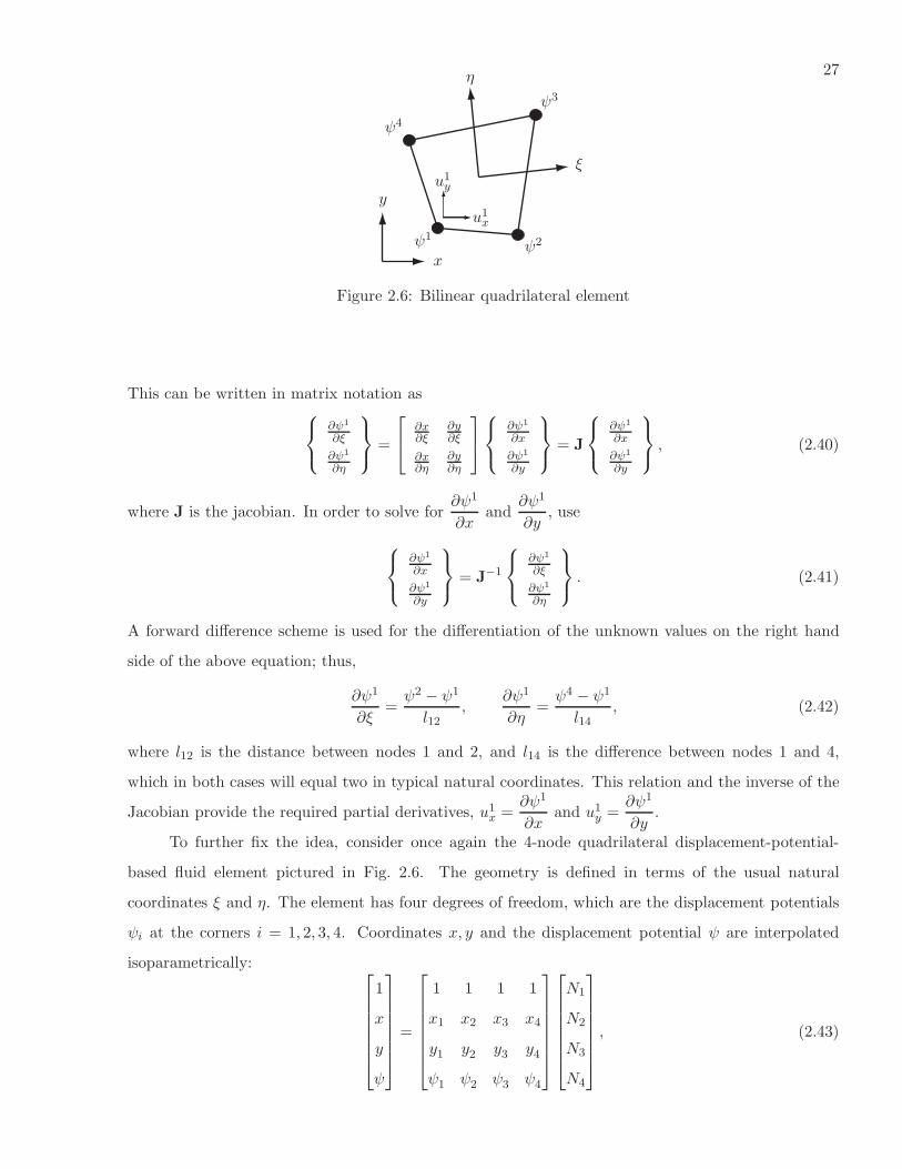
27
ψ1ψ2
ψ3
ψ4
x
yu1x
u1y
ξ
η
Figure 2.6: Bilinear quadrilateral element
This can be written in matrix notation as
∂ψ1
∂ξ
∂ψ1
∂η
=
∂x∂ξ
∂y∂ξ
∂x∂η
∂y∂η
∂ψ1
∂x
∂ψ1
∂y
= J
∂ψ1
∂x
∂ψ1
∂y
, (2.40)
where J is the jacobian. In order to solve for∂ψ1
∂xand
∂ψ1
∂y, use
∂ψ1
∂x
∂ψ1
∂y
= J−1
∂ψ1
∂ξ
∂ψ1
∂η
. (2.41)
A forward difference scheme is used for the differentiation of the unknown values on the right hand
side of the above equation; thus,
∂ψ1
∂ξ=ψ2 − ψ1
l12,
∂ψ1
∂η=ψ4 − ψ1
l14, (2.42)
where l12 is the distance between nodes 1 and 2, and l14 is the difference between nodes 1 and 4,
which in both cases will equal two in typical natural coordinates. This relation and the inverse of the
Jacobian provide the required partial derivatives, u1x =
∂ψ1
∂xand u1
y =∂ψ1
∂y.
To further fix the idea, consider once again the 4-node quadrilateral displacement-potential-
based fluid element pictured in Fig. 2.6. The geometry is defined in terms of the usual natural
coordinates ξ and η. The element has four degrees of freedom, which are the displacement potentials
ψi at the corners i = 1, 2, 3, 4. Coordinates x, y and the displacement potential ψ are interpolated
isoparametrically:
1
x
y
ψ
=
1 1 1 1
x1 x2 x3 x4
y1 y2 y3 y4
ψ1 ψ2 ψ3 ψ4
N1
N2
N3
N4
, (2.43)

28
with the bilinear shape functions N1 = 14(1− ξ)(1−η), N2 = 1
4 (1+ ξ)(1−η), N3 = 14(1+ ξ)(1+η) and
N4 = 14(1− ξ)(1+ η). Corner coordinate differences are abbreviated as xij = xi−xj and yij = yi− yj.
The Jacobian determinant is J = 14(A + A1ξ + A2η) with A = 1
2 (x31y42 − x42y31) is the area of the
quadrilateral, A1 = 12 (x34y12 − x12y34) and A2 = 1
2 (x23y14 − x14y23).
In terms of the node displacement 4-vector ψe = [ψ1 ψ2 ψ3 ψ4]T the Cartesian gradients ux =
∂ψ/∂x and uy = ∂ψ/∂y are given by
ux
uy
=1
8J
y24 y31 y42 y13
x42 x13 x24 x31
+
y43 y34 y12 y21
x34 x43 x21 x12
ξ +
y32 y14 y41 y23
x23 x41 x14 x32
η
ψe.
(2.44)
Evaluating (2.44) at the nodes yields
ueF =
ux1
uy1
ux2
uy2
ux3
uy3
ux4
uy4
=1
4
y24/J1 y41/J1 0 y12/J1
x42/J1 x14/J1 0 x21/J1
y23/J2 y31/J2 y12/J2 0
x32/J2 x13/J2 x21/J2 0
0 y34/J3 y42/J3 y23/J3
0 x43/J3 x24/J3 x32/J3
y34/J4 0 y41/J4 y13/J4
x43/J4 0 x14/J4 x31/J4
ψ1
ψ2
ψ3
ψ4
= DeF ψ
e, (2.45)
in which Ji are the corner Jacobians. These can be rapidly calculated from
4J1 = A−A1 −A2 = x14y21 − x21y14 = x42y14 − x14y42,
4J2 = A+A1 −A2 = x21y32 − x32y21 = x13y21 − x21y13,
4J3 = A+A1 +A2 = x32y43 − x43y32 = x24y32 − x32y24,
4J4 = A−A1 +A2 = x43y14 − x14y43 = x31y43 − x43y31.
(2.46)
The 8 × 4 gradient matrix DeF relates the Cartesian node displacement components to the node
displacement potentials. A similar transformation: ueF = DeF ψ
e can be constructed for any fluid
element based on the displacement potential element by appropriate differentiation and evaluation at
nodes.
Therefore, as the elements are assembled the global gradient matrix (D) can be created. How-
ever, instead of summing the contributions, an average must be taken. Once again, an example can
best explain. Assume the fluid is discretized with two bilinear quadrilateral elements as depicted in
Fig. 2.7. Notice for this example the element axes are aligned with the global axes.
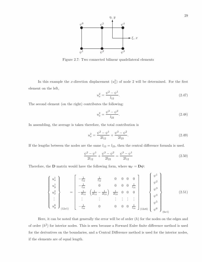
29
ψ1 ψ2 ψ3
ψ4ψ5ψ6
ξ, x
η, y
Figure 2.7: Two connected bilinear quadrilateral elements
In this example the x-direction displacement (u2x) of node 2 will be determined. For the first
element on the left,
u2x =
ψ2 − ψ1
l12. (2.47)
The second element (on the right) contributes the following:
u2x =
ψ3 − ψ2
l23. (2.48)
In assembling, the average is taken therefore, the total contribution is
u2x =
ψ2 − ψ1
2l12+ψ3 − ψ2
2l23. (2.49)
If the lengths between the nodes are the same l12 = l23, then the central difference formula is used.
ψ2 − ψ1
2l12+ψ3 − ψ2
2l23=ψ3 − ψ1
2l12(2.50)
Therefore, the D matrix would have the following form, where uF = Dψ:
u1x
u1y
u2x
...
u6y
(12x1)
=
− 1l12
1l12
0 0 0 0
− 1l16
0 0 0 0 1l16
− 12l12
(
12l12
− 12l23
)
12l23
0 0 0
......
......
......
− 1l16
0 0 0 0 1l16
(12x6)
ψ1
ψ2
ψ3
ψ4
ψ5
ψ6
(6x1)
(2.51)
Here, it can be noted that generally the error will be of order (h) for the nodes on the edges and
of order (h2) for interior nodes. This is seen because a Forward Euler finite difference method is used
for the derivatives on the boundaries, and a Central Difference method is used for the interior nodes,
if the elements are of equal length.

30
This representation of the fluid displacement, uF = Dψ, is then inserted into the total functional
equation, Eq. (2.35), to produce:
ΠTotal = uTS (1
2KSuS + CSuS + MSuS − fS)+
ψT (1
2DTKFDψ + DTMFDψ − DT fF )+
λTS (BTSuS − LSuB) + λTF (BT
FDψ − LFuB).
(2.52)
By applying it in this manner, the rotational modes that were associated with the mass matrix are
removed, because it did not use reduced integration. This concern was addressed with a projected
mass matrix by Chen et al. [21] and Kim et al. [74]. To simplify further derivations, the following
matrices are defined:
Mfd = DTMFD, Kfd = DTKFD. (2.53)
2.5 The Variation of the Energy Functional
The variation of the functional in Eq. (2.52) leads to the governing equations of the system.
δΠ(uS ,ψ,λS ,λF,uB) =
δuTS (MS uS + CSuS + KSuS + BSλS − fS)+
δψT (Mfdψ + Kfdψ + DTBFλF − DT fF )+
δλTS (BTSuS − LSuB) + δλTF (BT
FDψ − LFuB)+
δuTB(−LTSλS − LTFλF )
(2.54)
The sum of all the terms that are multiplied by the same differential are equated to zero, due to the
stationary condition. This leads to the following equation set:
KMS 0 BS 0 0
0 KMfd 0 DTBF 0
BTS 0 0 0 −LS
0 BTFD 0 0 −LF
0 0 −LTS −LTF 0
uS
ψ
λS
λF
uB
=
fS
DT fF
0
0
0
, (2.55)
where,
KMS = KS + CSd
dt+ MS
d2
dt2, KMfd = Kfd + Mfd
d2
dt2.
As noted by Park et al [101], we can make the following observations. First, the Lagrange multipliers
handle the interface interaction. Second, the partition subsystems’ boundary displacements (uS ,
uF = Dψ) are equated to the interface frame displacements (uB) as seen in row three and four of

31
Eq. (2.55). Finally, the Lagrange multipliers at a node obey Newton’s third law as seen in row five of
Eq. (2.55).
2.6 Summary
This chapter developed a set of governing equations for an acoustic fluid-structure interaction
system. The set of governing equations uses Localized Lagrange Multipliers for weak enforcement of
kinematic variables. The process begins by deriving energy functionals for the fluid, the structure, and
the interface of the two domains. The total functional of the system is the sum of the three energy
functionals. Components of the total functional are spatially discretized with finite element methods.
Standard linear shape functions are used for the displacement variables. However, a standard linear
shape function for the Lagrange multiplier field would lead to cumbersome integration of products of
functions on unrelated meshes. A simplification consists of taking multipliers as the conjugate forces
of the node displacements of nodes located on the interaction surface. If so, the multiplier shape
functions become simply node collocated delta functions.
Given the spatial discretization of the fluid, a gradient matrix is formed that allows for the
governing equations of the fluid to be transformed in terms of a displacement potential. This gradient
matrix is formed at the element level and assembled into a global matrix. However, the average
contribution of an element must be used for a specific displacement.

Chapter 3
Transient Concepts Using Localized Lagrange Multipliers
3.1 Introduction
This chapter presents transient methods using the previous developed coupling concept with Lo-
calized Lagrange Multipliers (LLM). First, a transient analysis is formed from the governing equations
developed with the use of the LLM. Then, other established transient methods are explored with the
use of LLM. Discretization errors and error measures for the transient analysis conclude this chapter.
The first section in this chapter develops a transient analysis method given the semi-discrete
governing equations, Eq. (2.55), with the LLM. The semi-discrete governing equations are integrated
in time using a partitioned analysis procedure. Direct time integration is used in preference to a
modal response analysis to preserve the ability to do nonlinear analysis, as in modeling cavitation.
The governing equations for the fluid, structure, and interface partitions are processed separately. At
each time step, the interface equations receive vector information from the interacting systems and
are algebraically solved for frame displacements and Lagrange multipliers. The multiplier results are
broadcast to the fluid and structure partitions, and used to update displacements and displacement
potentials for the next step. Any convenient solver for the fluid and structure partitions may be used,
and need not be the same. The interface set of equations have the potential to be ill-conditioned due
to scaling issues. This is resolved by scaling the interface system of equations.
The coupling concept of the LLM method can be used in other partitioned transient methods.
This is demonstrated in the next section of this chapter. The coupling equations for the LLM method
are used to develop relations from the fluid pressure to the structure force, and from the structure
displacements to the fluid displacements.
The chapter concludes with a section on error. Only the discretization error at the boundary
interface is discussed. Then, methods for measuring the transient error are discussed, which include
Geers’ comprehensive error factor [114] and energy differences at the interface.

33
3.2 Partitioned Transient Analysis
This section begins by developing a transient analysis of the system given the semi-discrete
governing equations, Eq. (2.55). This ultimately leads to an interface equation that is used for the
transient analysis. This interface equation solves for the Lagrange multiplier values at a certain time
step. These values are then used to update the structure and fluid variables (uS and ψ).
A time discretization of Eq. (2.55) is performed to begin the transient analysis. Thus, a numerical
time-stepping method for integration of the structure and fluid differential equations is used. The time
stepping method chosen for the problems in this study is the popular Newmark method [25], which
is heavily used in earthquake engineering. The Newmark method approximates the displacement and
velocity at the next time step (n+ 1) by
un+1 = un + ∆tun +1
2∆t2
[
2βun+1 + (1 − 2β)un]
,
un+1 = un + ∆t[
γun+1 + (1 − γ)un]
,
(3.1)
where ∆t is the time step value, n is the current time step, n + 1 is the next time step, β and
γ are parameters that determine the stability and accuracy characteristics of the algorithm under
consideration, see Table 3.2 [71].
Table 3.1: Properties of well-known members of the Newmark method
Method Type β γ Stability condition Order of accuracy
Trapezoidal Rule Implicit 14
12 Unconditionally 2
Linear Acceleration Implicit 16
12 Conditional 2
Fox-Goodwin Implicit 112
12 Conditional 2
Central Difference Explicit 0 12 Unconditional 2
Inserting the above approximations into the first and second rows of Eq. (2.55), and moving all
terms except the values of the structure displacement and the fluid displacement potential to the right
hand side yields
un+1S = FS(gn+1
S − BSλn+1S ), (3.2)
ψn+1
= FF (gn+1F − DTBFλ
n+1F ), (3.3)

34
where
FS =[
MS + ∆tγCS + ∆t2βKS
]
−1,
gn+1S = fn+1
S − CSunS + ∆t(1 − γ)unS − KSunS + ∆tunS +∆t2
2(1 − 2β)unS,
FF =[
Mfd + ∆t2βKfd
]
−1,
gn+1F = DT fn+1
F − Kfdψn + ∆tψn
+∆t2
2(1 − 2β)ψ
n.
(3.4)
Note that the values in gn+1F and gn+1
S are known, assuming that the forcing values are known.
Next, the second time derivative of rows three and four of Eq. (2.55) are evaluated at time step
(n+ 1). Then Eq. (3.2) and Eq. (3.3) are inserted for the values of un+1S and ψ
n+1to yield
BTSFSBSλ
n+1S + LSu
n+1B = BT
SFSgn+1S , (3.5)
BTFDFFDTBFλ
n+1F + LF un+1
B = BTFDFFgn+1
F , (3.6)
with unknown variables on the left hand side.
Finally, using the two above equations (3.5 and 3.6) and the remaining row of Eq. (2.55) at time
step (n + 1), the following equation set is obtained.
BTSFSBS 0 LS
0 BTFDFFDTBF LF
LTS LTF 0
λn+1S
λn+1F
un+1B
=
BTSFSg
n+1S
BTFDFFgn+1
F
0
(3.7)
This is referred to as the Interface Equation. Note that this equation set is only as large as the degrees
of freedom’s of the three state variables at the boundary; thus, the benefit in reducing the degrees of
freedom at the interface.
In order to solve the transient analysis, the Lagrange multipliers are determined by solving the
Interface equation, Eq. (3.7). These known values are then inserted into Eq. (3.2) and Eq. (3.3).
Therefore, the next time step values of the structure acceleration and the fluid second time derivative
of the displacement potential can now be determined. Then Eq. (3.1) can be used to obtain the
displacement and the displacement potential. With these values, the process can be repeated and
continued until the time period of the evaluation is completed. Notice that in this staggered procedure
there is no prediction step, which can cause loss of accuracy and instability. However, care must be
taken in solving the Interface equation, Eq. (3.7), because it can be ill-conditioned. Therefore, the
Interface equation set is scaled in a manner similar to the method by Yue [127] and discussed in
Section 3.2.1 to resolve the ill-conditioning. Finally, it is pointed out that this transient procedure
allows for the use of different solvers for the fluid system and the structural system. A diagram
illustrating the time stepping procedure for the Trapezoidal Rule is depicted in Fig. 3.1.

35
InterfaceInterfaceInterface
StructureStructure
FluidFluid
etc.
etc.
t0 t1 t2time steptime steptime step
f1 f2 f3
ψ1
= FF (g1F − DTBFλ
1F ) ψ
2= FF (g2
F − DTBFλ2F )
u1S = FS(g1
S − BSλ1S) u2
S = FS(g2S − BSλ
2S)
ψ1, ψ
1, ψ1 ψ
2, ψ
2, ψ2
u1S , u1
S, u1S u2
S , u2S, u2
S
λ1F , f1
λ2F , f2
λ1S , f1 λ2
S , f2
Figure 3.1: Graphical representation of the time stepping procedure for the LLM method.
36
If the nonlinear effect of cavitation is to be included, then it is recommended to use the Central
Difference method. This is recommended because of the removal of the stiffness matrix in the matrix to
be inverted, to be discussed in Section 8.2. Unfortunately, care must be taken if the Central Difference
method is used, because of the stability concerned with the size of the time step value. In the Central
Difference Method, which is an explicit direct integration method, the time step must be small enough
that information does not propagate more than the distance between adjacent nodes during a single
time step. This is referred to as the CFL condition [29]. A convenient measure to assure this for fluids
is the Courant number [51].
The transient analysis provides some clear benefits of the LLM method. First, the partitioned
analysis can be solved without the normal need for a prediction step. This is advantageous because
typically the prediction step in staggered integration procedures can cause instability. Second, the
fluid, structure, and the interface equation can be solved by separate solvers tailored to the particular
system. Third, the fluid and the structure can be solved in parallel. Finally, the interface equation
will generally be a smaller system set to solve and should be faster. It should also be noted that
the transient analysis is solved for the second time derivatives of the state variables, because of the
advantage of determining cavitation, which is discussed in Section 8.2
3.2.1 Scaling the Interface Equation
As previously mentioned, care must be taken when evaluating the Interface Equation, Eq. (3.7),
because it can be an ill-conditoned equation. The ill-conditioned nature is of great concern in solving
the linear algebra system given by the Interface Equation, because a small perturbation in the right
hand side vector can cause a large change in the solution vector [3]. The ill-conditioned nature arises
because the values of the interface equation matrix vary greatly in size, due to the heterogeneous
physical systems and the magnitude of the connection matrices (L). Large loss of significance errors
will be introduced and the propagation of rounding errors will be worse, due to the considerable
difference in values of the interface equation matrix [3]. Therefore, to avoid the problem, the interface
equation matrix is scaled so that the values are near one. Dongarra et al. [33], Forsythe and Moler
[53], Atkinson [3], and Golub and Van Loan [60] among others, have addressed the scaling issue of
matrices. In this subsection, a method for scaling the interface equation is shown that extends the
work of Yue and Park [127].
Yue mentions two approaches for scaling the ill-conditioned matrices [127]. The first approach
is to scale the interface force (Lagrange multipliers) along the partitioned boundaries [62, 100]. This

37
begins by modifying the constraint functional with normalization matrices DS , DF , such has:
Πconstraint = λTS DS(BTSuS − LSuB) + λTF DF (BT
FDψ − LFuB). (3.8)
This ultimately leads to a normalization of the interface equation as shown by Gumaste et al. [62] and
can be illustrated by inserting the above constraint function into Eq. (2.52) and following the steps in
Section 2.5.
The second approach is the displacement scaling method. The basic idea is to scale the mag-
nitude of the diagonal terms of matrices (BTSFSBS and BT
FDFFDTBF ) to the order of one. This
causes a special need for modifying the third equation (Newton’s third law) of the interface equation,
Eq (3.7), and here is the extension to Yue’s work. In modifying the third equation, the objective is
to either average the majority of the terms to near one, or to take the maximum term and scale it to
one and scale all others by the scaling factor. The interface equation is shown below again for clarity.
BTSFSBS 0 LS
0 BTFDFFDTBF LF
LTS LTF 0
λn+1S
λn+1F
un+1B
=
BTSFSg
n+1S
BTFDFFgn+1
F
0
.
First, the scaling of the matrices (BTSFSBS and BT
FDFFDTBF ) in the interface equation matrix
is done in the following manner. Define the following for clarity:
FS = BTSFSBS ,
FF = BTFDFFDTBF ,
GS = BTSFSg
n+1S ,
GF = BTFDFFgn+1
F .
(3.9)
Scaling matrices for the terms (BTSFSBS and BT
FDFFDTBF ) can be created as
SS =[
(diag(FS))12
]
−1,
SF =[
(diag(FF ))12
]
−1,
(3.10)
where diag() refers to using only the diagonal components of the matrices. Therefore, the matrix
multiplication STS FSSS will result in a matrix with ones on the diagonal, and similarly for STF FFSF .
Hence, the first and second equation of the interface equation matrix would have the form:
STS FSSS(S−1S λ
n+1S ) + STSLS(un+1
B ) = STSGS ,
STF FFSF (S−1F λ
n+1F ) + STFLF (un+1
B ) = STF GF ,(3.11)
38
where the equations are pre-multiplied by the transpose of their respective scaling matrices and the
inverse of the scaling matrices are used so that unity on the diagonals is obtained. Note that taking
the inverse of the scaling matrices is rather simple, since the matrices only consist of diagonal terms.
In the above equation, Eq. (3.11), the term STSLS and STFLF have now become orders of magni-
tude away from unity. For example, if the structure is made from standard concrete, then the values
in the matrix STSLS are of the order of 105. Thus, it is desirable to scale these values to one as
well. However, this can become complicated because of the non-matching meshes and the use of the
zero-moment rule. The use of the zero-moment rule can create a boundary discretization that has
a different number of degree of freedoms than either the structure interface boundary or the fluid
interface boundary, which precludes the use of the method by Yue [127]. Once again, the objective
is to scale the numbers of these matrices to the order of one. This can be accomplished by using the
following scaling parameter:
s =1
2
(
ni∑
1
nj∑
1
|(STSLS)ij |nsz
+
ni∑
1
nj∑
1
|(STFLF )ij|nfz
)
, (3.12)
where ni and nj are the rows and columns of the respective matrices, and nsz and nfz are the number
of nonzero values of the respective matrices. A square scaling matrix for the concerned matrices STSLS
and STFLF can be created with this parameter as:
(SB)ii =1
s. (3.13)
Thus, it only has values on the diagonal and its size is the size of the column of LF or LS, which is the
number of degree of freedoms accounted for on the interface boundary with the normal component
taken into account.
Therefore, the three equations of the interface equation are scaled to the order of one, and are
written as follows:
STS FSSS(S−1S λ
n+1S ) + STSLSSB(S−1
B un+1B ) = STSGS ,
STF FFSF (S−1F λ
n+1F ) + STFLFSB(S−1
B un+1B ) = STF GF ,
STBLTSSS(S−1S λ
n+1S ) + STBLTFSS(S−1
S λn+1F ) = 0.
(3.14)
In matrix form:
STS FSSS 0 STSLSSB
0 STF FFSF STFLFSB
STBLTSSS STBLTFSS 0
S−1S λ
n+1S
S−1S λ
n+1F
S−1B un+1
B
=
STSGS
STF GF
0
. (3.15)
The original interface equation, Eq. (3.7), will be used and referenced in the remainder of this
study to avoid clutter. However, it should be noted that this matrix has been scaled with success for

39
the problems in this study in the above manner. Some simple comparisons showing the advantage of
this scaling procedure are discussed in Chapter 6.
3.3 Inclusion of Concept for other FSI Methods (i.e. CASE)
It is sufficient to say that many organizations already have an acoustic fluid code and a structure
code that they are content with using, but want to be able to handle non-matching meshes. This can
be accomplished by using the salient features of the LLM method to develop a relationship between
the structure’s boundary displacements and the fluid’s boundary displacements as well as the systems
boundary forces. In most typical FSI codes, the structure displacement is passed to the fluid and the
fluid passes the pressure to the structure; thus, two relations are provided. The first is the relation
between the fluid’s pressure and the structure’s force at the interface boundary. By relating these to
the Lagrange multipliers and using the relation between the Lagrange multipliers the interface patch
test is satisfied. The second relation is between the subsystem’s interface displacements and can be
found from the relation of the subsystem’s forces.
3.3.1 Relation Between Fluid Pressure and Structure Force
In order to assure that the interface patch test is satisfied a relationship between the fluid
pressure at the boundary and the Lagrange multiplier needs to be determined. Given the fact that the
interface constraint functional is in terms of energy, the normal value of the fluid’s Lagrange multiplier
can be thought of as being equal to the opposite of the fluid’s pressure determined at the boundary
pFB, which is in accordance with Newton’s third law.
λnF = −pFB, (3.16)
where the superscript n refers to the normal value in this section, and should not be confused with
any time-stepping value. In addition, the structure’s normal value of the Lagrange multiplier can
be thought of as the normal value of the structure force being applied at the structures interface
boundary. Therefore, it is only necessary to determine the normal value of the structure’s Lagrange
multiplier in terms of the fluid normal value of the Lagrange multiplier. Once the normal value of
the structure’s Lagrange multiplier is known then the force acting on the structures wetface can be
determined by calculating the average normal at the structure’s node and multiplying this vector to
the relevant normal structural Lagrange multiplier value.
Therefore, the interface constraint energy functional is used to develop a relation between the
partitioned FSI subsystems’ Lagrange multipliers. The interface constraint energy functional is rewrit-

40
ten below for convenience.
ΠB =
∫
ΓF B
λF ini(uF ini − uBini)dΓFB +
∫
ΓSB
λSini(uSini − uBini)dΓSB .
As noted for an acoustic fluid structure interaction, it is desirable to have the Lagrange multipliers in
terms of the normal components. Hence, only the normal values are needed, and the boundaries can
use the normal values as their primary variables to be discretized.
ΠB =
∫
ΓF B
λnF i(unF i − unBi)dΓFB +
∫
ΓSB
λnSi(unSi − unBi)dΓSB. (3.17)
The primary variables (Lagrange multipliers and displacements) can be discretized as before except
with the realization that the normal vector is not needed and there is only one-degree of freedom at
each node due to the normal value being the variable component.
ΠB = (λnF )T
([
∫
ΓeF B
NTλFNFdΓFB
]
unF −[
∫
ΓeB
NTλFNBdΓB
]
unB
)
+
(λnS)T
([
∫
ΓeSB
NTλSNSdΓSB
]
unS −[
∫
ΓeB
NTλSNBdΓB
]
unB
)
,
(3.18)
where it assumed that the integrations on the elements are assembled into global matrices, which
produces:
ΠB = (λnF )T(
(BnF )TunF − LnFunB
)
+ (λnS)T(
(BnS)TunS − LnSu
nB
)
. (3.19)
The variation of the interface constraint energy functional leads to the following set of equations at
the interface,
δΠB = δ(λnF )T(
(BnF )TunF − LnFunB
)
+
δ(λnS)T(
(BnS)TunS − LnSu
nB
)
+
δ(unB)T(
−(LnF )TλnF − (LnS)TλnS)
+
δ(unF )T (BnFλ
nF )+
δ(unS)T (BnSλ
nS) .
(3.20)
The third equation in Eq. (3.20) can be used to find the relation between the two normal
Lagrange multipliers.
λnS = −[
LnS(LnS)T]−1
LnS(LnF )TλnF (3.21)
This then provides the relation between the fluids pressure and the acting normal force at the interface
boundary of the structure, fSB;
fnSB =[
LnS(LnS)T]−1
LnS(LnF )TpFB. (3.22)
41
By using this relationship, a constant stress can be passed from the fluid subsystem to the structure
subsystem. However, there is the possibility that the matrix[
LnS(LnS)T]
is singular. This can happen
when the structure mesh is refined within each fluid element. There are two methods to get around
this issue. The first is to obviously remesh. The second is to use a relationship between the fluid
displacements and the structure displacements from Eq. 3.20, then with the use of the virtual work at
the interface, a relation between the Lagrange multipliers can be determined as discussed in the next
section. However, using the displacements values relation does not assure that the interface patch test
is passed.
3.3.2 Relation between Subsystems’ Boundary Displacements
In many acoustic FSI methods, there is a need to know the discretized fluid’s boundaries nor-
mal displacement in terms of the discretized structures normal displacement. For instance, in the
CASE method [114] (see Appendix A) the normal displacement at the boundary effects the boundary-
interaction vector.
be =
∫
Γe
φ∇ψ · nidΓ =⇒∫
Γe
φuF i · nidΓ, (3.23)
where φ is a column vector composed of 1-D, N th-order-polynomial basis functions.
Therefore, the first and second equations of Eq. (3.20) can be used to develop a relationship
between the fluid’s normal boundary displacements and the structure’s normal boundary displacements
such as
unFB = LnF[
(LnS)TLnS]−1
(LnS)TunSB, (3.24)
where unFB and unSB refer to the normal displacements of the fluid and the structure respectively at
the boundary.
Therefore, given the structure’s normal displacements at the nodes of the structure boundary,
the fluid’s normal displacement at the nodes of the fluid boundary are determined. The structure’s
normal component can be determined by the known structure’s displacements of an element and
creating the normal components from these values. The normal value at a node is the average of the
normal values of the elements surrounding the node.
When maintaining the normal component in the integration of the connection matrices L, i.e.
for the structure,
LS =
∫
ΓeB
NTλSn
eneTNB dΓeB (3.25)
a problem can arise in the inversion of the matrix[
(LS)TLS]
−1, because it has the potential to become
singular. Therefore, it is imperative to use the normal values of the displacements for the derivation.

42
Another option to determine the relation between the subsystems boundary forces is to use
the relation between the susbsystems’ boundary displacements and the principle of virtual work.
This results in using the transpose of the matrix created by the relation between the normal fluid
displacement and the normal structure displacement [38] for the relation among the forces. This can
be seen by examining the virtual work on the boundaries.
δWFB = (λnF )TunFB, (3.26)
where W is the work and FB refers to the fluid boundary. Inserting
unFB = LnF[
(LnS)TLnS]−1
(LnS)TunSB = RnFSu
nSB ,
where RnFS is the relation from the structure normal displacements to the fluid normal displacements,
into Eq. (3.26) provides
δWFB = (λnF )TRnFSu
nSB. (3.27)
The virtual work along the structure boundary is given by
δW SB = (λnS)TunSB. (3.28)
Therefore, by equating Eq. (3.27) and Eq. (3.28) it can be seen that
λnS = (RnFS)TλnF . (3.29)
This relationship can be used for the forces, but it does not guarantee that the patch test will be
satisfied. Also, there is the issue where the matrix[
(LnS)TLnS]
can become singular. It can become
singular in the opposite case of the previous one used for the Lagrange multiplier’s relation for it would
be come singular if the fluid mesh is refined within a structure element.
In conclusion, the Lagrange multiplier relation should be used for the force relation in order to
pass the interface patch test. Unfortunately, this can become an issue if the structure is more refined
then the fluid. However, there is a method to get around the issue, but can result in non-conservative
forces at the interface.
3.4 Error/ Accuracy
This section begins with a discussion on the order of the discretization error in strain associated
with LLM method previously derived. Here, we concentrate on the error associated with spatial
discretization at the interface boundary, because the method is capable of being implemented with

43
any time integration, which would dictate the error due to the time discretization. Then posteriori
error estimates are mentioned that are used in the remaining chapters.
Fortunately, the Mortar method, discussed in Appendix B.1, has resulted in significant studies
on the error associated with the method [8, 112, 125, 126]. The Mortar method achieves coupling
between two non-overlapping domains, Ωi, Ωj, by using a Lagrange multiplier to weakly enforce the
constraint ui − uj = 0 along the interface boundary [4].
∫
Γλ(ui − uj)dΓ = 0. (3.30)
This method provides a discrete solution that satisfies optimal error estimates with respect to nat-
ural norms [8]. For instance, if the subdomains (Ωs) are discretized with linear finite elements on a
mesh with a characteristic size hs, then the global discretization error of the coupled problem grows
asymptotically as O(hs). This error was derived with the following assumptions.
• The domain Ω is partitioned into non-overlapping polygonal subdomains Ωs.
• The interface Γij of two subdomains intersection Ωi ∩ Ωj can be decomposed into a set of
disjoint straight line pieces γi.
• The triangulations over the different domains Ωs are assumed independent of each other, with
no compatibility enforced across interfaces.
• The mortar discretization is the trace of the triangulation from one of the domains Ωs, and it
uses the same piecewise polynomial interpolation over the element.
Given item four of the assumptions, where the discretization of the Lagrange space is equal to one of the
domains, it is determined that this is the same for the LLM method across the interface boundary to
each subdomain. Therefore, the global discretization error for the LLM method grows asymptotically
as O(hS) +O(hF ) +O(hB) with linear shape functions used for the Lagrange multipliers as described
in Section 2.3.4. In other words, the interface error induced by the LLM method on the solution is
not worse than the local fluid, structure, and boundary discretization errors.
However, the above error is associated with linear shape functions for the Lagrange multipliers
given the fluid and structure formulations in this study. The error for the formulation developed with
Dirac delta functions for the shape functions are assumed to be different. Farhat et al. [38] note
that using an interpolation method, where one subdomain’s interface Γi values are interpolated to the
interface of another Γj, gives a discretizatioin error of the coupled domains that grows asymptotically
as O(√hi). In essence, the LLM method with Dirac delta shape functions for the Lagrange multipliers,

44
ultimately interpolates the values of the subdomains to the interface frame, see Appendix B.2. Thus,
the discretization error of the LLM method with Dirac delta shape functions grows asymptotically as
O(√hF ) +O(
√hS) +O(
√hB) in strain.
The error is not mathematically optimal, but it will be shown to be sufficient for problems in
this study. In Appendix C, the discretization error for the two dimensional problems is shown to
be of order O(h2f + h2
s + h2b) in displacements, where the displacement variables at the interface are
interpolated with linear shape functions, and the intersection of the subdomains is composed of linear
disjoint segments. The remainder of the Chapter provides error measures used to evaluate the LLM
method in the problems of this study.
3.4.1 Geer’s C-Error Method
Geers’ comprehensive error factor [114] is used to quantify the error of a transient response
history relative to an accepted benchmark solution. The comprehensive error factor is given by C =√M2 + P 2, in which
M =√
ϑcc/ϑbb − 1, P =1
πarccos(ϑbc/
√
ϑbbϑcc),
ϑbb =1
t2 − t1
∫ t2
t1
b2(t)dt, ϑcc =1
t2 − t1
∫ t2
t1
c2(t)dt,
ϑbc =1
t2 − t1
∫ t2
t1
b(t)c(t)dt,
(3.31)
where c(t) is a candidate solution in the form of a response history, b(t) is the corresponding benchmark
history, and t1 ≤ t ≤ t2 is the time span of interest. The integrations are done numerically with the
composite Simpson’s rule [75], for this study. M is the magnitude error factor, which is insensitive to
phase discrepancies, and P is the phase error factor, which is insensitive to magnitude discrepancies.
3.4.2 Energy Error
Before moving to the numerical experiments, another type of error measurement that will be
used throughout the experiments should be discussed. This error is the energy or momentum difference
at the interface. If the interface is viewed as being a closed system, then the energy gained or released
on one side of the interface frame is equal to the energy lost or absorbed by the other side of the
interface. Thus, the difference in the energy on the two sides of the interface is used for an error
measurement. Two types of error can be examined for the LLM method. The first is the difference at
the interface frame.
W (n)interror = uTB(−LTSλS − LTFλF ), (3.32)

45
where n refers to the time step, and int is the for the interface frame. This will provide a graphical
representation of the error at the interface throughout the time span of interest. This difference
will be used to notice any error that is really introduced by the scaling of the interface equation,
see Section 3.2.1, for the Lagrange multipliers are specifically solved only at the interface equation.
According to the third equation of the Interface equation, Eq. 3.7, mathematically the system is
conservative at the boundary as the forces are equal and opposite in accordance with Newton’s third
law. However, when using the LLM transient method there is a minor error noticed with the above
equation that is not present when using the CASE method with the LLM concept for the non-matching
meshes. This indicates that the scaling is introducing a little error into the system. This is to be further
discussed in Chapter 6.
The next error is associated with the energy at the boundary of the different domains. In this
error, the energy at one subdomain’s boundary is compared with the energy at the other subdomain.
W (n)suberror = λTS (BTSuS) + λTF (BT
FDψ), (3.33)
where sub refers to the error associated with difference between energy on the different subdomains.
Once again, this is provided at each time step and will be used for visual purposes. This error is
associated more with the LLM method as it looks at the energy difference between the subdomains’
boundaries. Also, note that any error created by the gradient matrix, D, will be introduced into this
measurement. In addition, the plus sign is used because the Lagrange multipliers are theoretically
equal and opposite at the interface frame.
An energy difference can also be used with other FSI codes that incorporate the LLM method,
see Section 3.3. This is simply the same error as mentioned above for the energy difference at the
subdomains’ boundaries.
W (n)CASEerror = fTSB(uSB) − fTFB(uFB), (3.34)
where fSB is the force at the structures wet face produced from the fluid pressure converted to the
structure boundary DOF by some method, fFB is the force at the fluid dry face from the fluid pressures,
uSB is the structure displacements at the wet face, and uFB is the fluid displacements at the dry face.
In a staggered integration procedure the correct time step value of the uSB needs to be used, which is
the predicted value. This error measure is used to graphically compare different non-matching mesh
techniques.

46
3.5 Summary
In this chapter, the Localized Lagrange Multiplier (LLM) method is extended for use in an
acoustic fluid-structure interaction (FSI). The main feature was the transient analysis in the time
domain that was developed. Conveniently, this transient analysis allows for a partitioned method that
has the potential for an always stable method, if implicit transient analysis methods are chosen for
the time integration.
However, if a cavitation analysis is required, then it is more computationally efficient to use
the explicit time integration method known as the Central Difference method, to be discussed in
Chapter 8. Ultimately, this cavitation analysis leads to significant computational inefficiency when
compared to the Cavitating Acoustic Spectral Element (CASE) method [114], to be discussed in
Chapter 8. Therefore, the ability to couple non-matching meshes with the LLM method is extended
to the CASE method. However, this has limitations in that it may not always pass the interface patch
test.
Finally, it was noted that the LLM method has the potential for optimality in regards to the
discretization error. However, a simpler integration procedure was provided using Dirac delta shape
functions for the Lagrange multipliers that affected the discretization error. Nonetheless, this simpler
integration procedure is used throughout this study to help evaluate the method. The rest of the
chapters in this study are used for validation and comparison of the LLM method.

Chapter 4
Validation of Fluid Code: Pressure on Dam Face
4.1 Introduction
This chapter is intended to show that the fluid formulation derived for the LLM method with
the gradient matrix can provide accurate results. In the derivation of the fluid formula, Section 2.4, it
is shown that the discretization error of the fluid displacement is greatest at the edges of the domain
O(h), and the order of the discretization error is O(h2) for interior nodes. Therefore, the pressure on
the edge of the fluid is compared between an analytical model and the derived computational model.
In addition, this chapter provides an analysis with the use of silent boundaries. There is also a brief
section on the inclusion of surface waves.
4.2 Problem Description and Analytical Solution
The problem studied is a rigid dam excited by an earthquake, uq, as depicted in Fig. 4.1. This
problem was studied by Chopra [23], where an analytical solution was determined for the pressure on
the dam face. Chopra made the following assumptions during this study. The effect of the length of
the fluid is negligible for L/H > 3, where L is the length of the fluid and H is the depth of the fluid.
In addition, the effect of surface waves could be ignored with little loss of accuracy as long as the
depth is greater then 100 ft, for a typical ground motion period below three seconds.
Given the above assumptions, the following analytical form of the pressure was determined by
Chopra [23]:
p(0, y, t) =4ρc
π
∞∑
n=1
(−1)n−1
2n− 1cosλny
∫ t
0uq(τ)Joλnc(t− τ)dτ, (4.1)
where ρ is the fluid density, c is the velocity of sound in the fluid, λn = (2n − 1)π/(2H), y is the
vertical height on the dam face, H is the depth of the fluid, Jo is the Bessel function of the first kind
of order zero, t is time, and uq(τ) is the given earthquake acceleration. Parameters for these values are
shown in Table 4.1. The El Centro earthquake of May 18, 1940, was chosen as the excitation for this
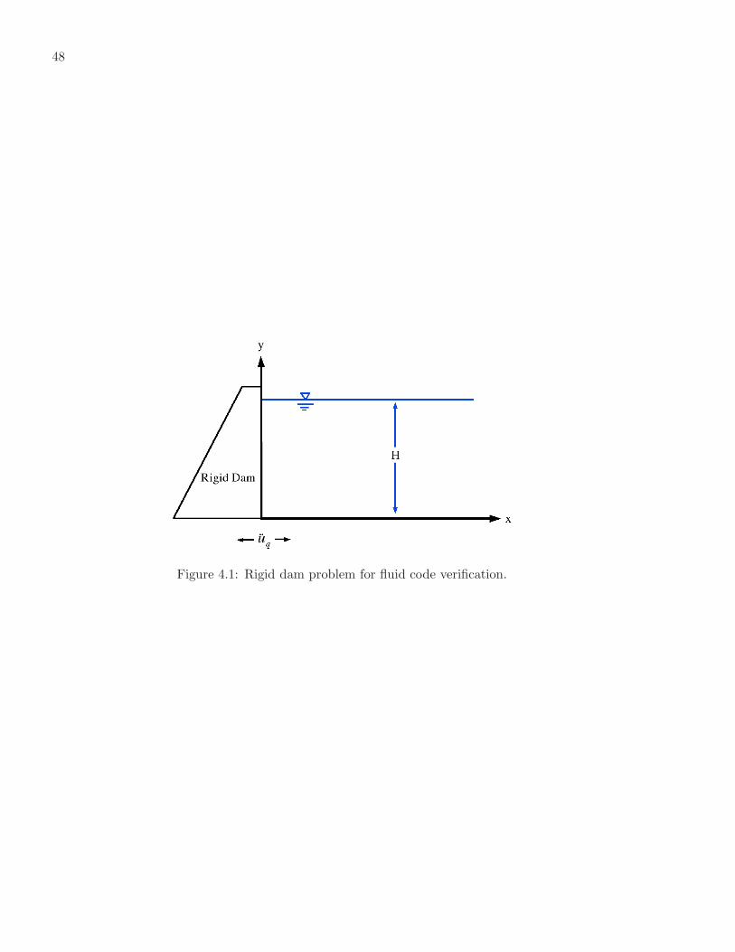
48
Figure 4.1: Rigid dam problem for fluid code verification.

49
problem, and only the x-direction of the acceleration was used. This provided the analytical solution
shown in Fig. 4.2 for the first eight seconds of the earthquake.
ρ 1000 kg/m3
c 1500 m/sH 80.0 my 40.0 m
time duration 8.0 s
Table 4.1: Parameters for the pressure on the dam face problem.
4.3 Fluid Code Validation
Given the analytical solution, a comparison with computational models can be conducted. In
these models, the pressure is computed in elemental gauss points surrounding the point of interest,
then interpolated to the point. The point of interest is on the dam face located forty meters from
the bottom of the fluid. The pressure in the element is determined with the use of the displacement
volume strain matrix and the fluid displacements. In the current finite element discretization scheme
the pressure inside an element, and at a certain location in the element, can be determined by the
following relation that is typically used for the computation of stress in structures.
p = −ρF c2BvsueF , (4.2)
where ueF is found from the global displacements (uF = Dψ), and Bvs is the displacement volume
strain matrix at a particular location in an element [36].
Bvs = ∇ ·NF (4.3)
This can be saved during the initial calculation of the stiffness matrix of the fluid. However, reduced
integration is used and thus, the pressure at the center of the element will be determined. As noted
by Dow [34], a smoothed solution of the pressure would more closely approximate the actual pressure
solution. Therefore, the pressure is found at gauss points for full integration. Given these values, the
element pressure at the desired location is interpolated from the gauss points. If the desired location
is on an edge of element, then the average from the neighboring elements is used. This method is
used, because it requires the gradient matrix (uf = Dψ) which is one of the new components of the
fluid formulation and needs to be verified.

50
0 1 2 3 4 5 6 7 8−2
−1.5
−1
−0.5
0
0.5
1
1.5
2
2.5x 10
5
Time (seconds)
Pressure
Figure 4.2: Analytical pressure on the rigid dam.
Figure 4.3: Fluid mesh with a characteristic length of 20 m.

51
The verification begins by examining three fluid meshes. The first fluid mesh is depicted in
Fig. 4.3, where the element length is twenty meters. The second mesh reduces the characteristic
length by half to ten meters, and the third mesh again reduces the length by half to five meters.
In order to evaluate the fluid formulation for the LLM method, three figures are provided for
visual comparison, please see Fig. 4.4, Fig. 4.5, and Fig. 4.6. In addition, on each figure is the C-error,
M-error, and P-error. These error measures are explained in Section 3.4. As can be seen, the error
is reduced for each refined mesh. The magnitude error is greater then the phase error, which could
be associated with the silent boundary and extending the period of analysis past three seconds as
recommended in Chopra’s study.
0 1 2 3 4 5 6 7 8−3
−2
−1
0
1
2
3
4x 10
5
Time (seconds)
Pre
ssur
e (P
a)
C−Error = 0.46; M−Error = −0.39; P−Error = 0.24
LLMAnalytical
Figure 4.4: Pressure on dam face with a fluid characteristic length of 20 m.
4.4 Incorporation of Silent Boundaries
An issue that needs to be considered for problems in this work is that of silent boundaries (non-
reflecting boundaries). Silent boundaries are needed to truncate the domain volume to a finite extent.
Thus, this section explains the incorporation of silent boundaries with the fluid formulation and the
structure formulation as depicted in Eq. (2.54). It is desirable for the boundary to perfectly radiate
outgoing waves (no spurious reflections). In addition, it is desired that the boundary be as close to

52
0 1 2 3 4 5 6 7 8−2.5
−2
−1.5
−1
−0.5
0
0.5
1
1.5
2
2.5x 10
5
Time (seconds)
Pre
ssur
e (P
a)
C−Error = 0.31; M−Error = −0.26; P−Error = 0.18
LLMAnalytical
Figure 4.5: Pressure on dam face with a fluid characteristic length of 10 m.
0 1 2 3 4 5 6 7 8−2.5
−2
−1.5
−1
−0.5
0
0.5
1
1.5
2
2.5x 10
5 C−Error = 0.26; M−Error = −0.20; P−Error = 0.17
Time (seconds)
Pre
ssur
e (P
a)
LLMAnalytical
Figure 4.6: Pressure on dam face with a fluid characteristic length of 5 m.

53
the finite structure as possible for computational efficiency.
The Perfectly Matched Layer (PML) method [9] would meet these requirements. This method
was developed in the frequency domain for electromagnetic wave absorption. It has been found that the
PML absorbing boundary condition provides much higher absorption than other previous absorbing
boundary conditions in finite-difference methods [82]. Hence, much work as been done to extend the
method to the finite difference time domain. Several authors, [22, 128, 82], have extended the method
for elastic waves with the finite difference method. Geers and Qi, [57] demonstrated the ability of the
PML to be used in acoustics with the finite difference method in the frequency and the time domain.
They also provided criteria for using the PML in acoustics. Extensions into the finite element method
have been performed for elastodynamics by several as well, [6, 7, 79, 81] in the frequency domain.
Basu et al., [7], were able to develop the PML method for finite elements in the time domain.
However, it has been found that the implementation burden of the PML would not be justified
in the problems of this study. Brahtz and Heilbron [17], and Calayir and Karaton [19], mention that
the effect of the radiating condition on the solution is generally negligible if the reservoir length is
taken three or more times then the depth of the reservoir. Since it is desired to capture the majority
of the cavitation region in the fluid computational domain, meeting the requirement for the length of
the reservoir is desirable. In regards to the structure, 5% Rayleigh damping is present in the domain
and this helps with the attenuation of the elastic wave.
However, a silent boundary is still provided for problems in this study. The plane wave approxi-
mation is provided for the fluid. The structure’s silent boundary uses the Viscous Damping Boundary
method (VDB) of Lysmer and Kuhlemeyer [83]. This was tested by comparing extended models that
would not effect the response in the time period of the two dimensional dam problems without fluid
to a truncated model with the VDB. Here it was found that a length of two times the height of the
dam provided negligible effects on the solution of displacements on the dam face. It has been noted
these absorbing boundary conditions are only approximated, and small reflections from the boundaries
should be expected. Komatitsch et al., [77] mentions that the amplitude of these reflections is of the
order of a few percent of the amplitude of the direct wave. Obviously, these conditions are optimal for
waves impinging normal to boundary and rapidly become less accurate when the angle of incidence
differs from the normal [26].
The simplest method to be incorporated into the above derived fluid formulations would be
the use of a plane wave approximation (PWA) for the silent boundary. It is valid for short acoustic
wavelengths (high frequencies) and is useful for modeling early stages of the transient interaction [58].
The PWA is chosen over the Doubly Asymptotic Approximation (DAA), [56, 59], because the waves

54
are assumed to behave as a plane wave and the extent of the fluid length previously mentioned. The
PWA relates the pressure to the velocity by the following:
p = ρF cun, (4.4)
where c is once again the fluid speed of sound, p is the pressure, and un is the normal component of
the velocity at the boundary [42]. In the energy functional of the fluid, there is a term that is related
to the surface traction. In this term, the PWA can be introduced through the relation between the
traction and the pressure
TF i = −pni. (4.5)
This ultimately can lead to a damping term that is added to the fluid equations as the following:
CeF =
∫
ΓFnrb
cρFNTneneTNdΓFnrb, (4.6)
where ΓFnrbis the silent boundary, n is the normal vector at that boundary, and N is a standard
linear shape function. In order to use the displacement potential as the fluid state variable, the fluid
damping matrix is modified by the gradient matrix (D), as was done to the fluid stiffness and mass
matrix, see section 2.4.
Cfd = DTCFD (4.7)
This then fits into the variation of the systems energy functional, Eq. (2.54), as
δΠ(uS ,ψ,λS ,λF ,uB) =
δuTS (MSuS + CSuS + KSuS + BSλS − fS)+
δψT (Mfdψ + Cfdψ + Kfdψ + DTBFλF − DT fF )+
δλTS (BTSuS − LSuB) + δλTF (BT
FDψ − LFuB)+
δuTB(−LTSλS − LTFλF ).
(4.8)
A partitioned transient analysis can then be performed as discussed in section 3.2.
A silent boundary for the structure is included by the simple Viscous Damping Boundary method
(VDB) of Lysmer and Kuhlemeyer [83]. The VDB is similar to the plane wave approximation method
in that the VDB uses the concept of applying viscous dampers to the DOF on the boundary element.
However, for an elastic media, such as soil, there are primary waves and secondary waves that travel
through the media. Thus, the speed of these waves is used instead of the speed of sound in the fluid,
which was used for the PWA. Primary waves are compression waves that travel through solids, liquids,
and gases. Secondary waves are shear waves that only travel through solids.

55
In order to develop a boundary condition that ensures that all energy arriving at the boundary
is absorbed, Lysmer and Kuhlemeyer [83] found that the most promising expression for the boundary
condition is expressed by the following equations.
σzz = aρVpuz Primary wave
τzx = bρVsux Secondary wave
τyz = bρVsuy Secondary wave
(4.9)
These equations are formulated for an incident wave consisting of a primary and secondary wave that
act at an angle θ from the z-axis as shown in figure (4.7) [55]. In the above equations, ρ is the density
of the media, ux, uy, uz represent the velocities in the x,y,z-direction, Vp and Vs are the velocities of the
primary and secondary waves, and a and b are dimensionless parameters. For small incident angles
(θ < 30), the most effective value for the dimensionless parameters (a and b) is one [83].
Figure 4.7: Viscous Damping Boundary concept [55].
The primary and secondary velocities can be computed as
Vp =
√
(1 − ν)E
(1 − 2ν)(1 + ν)ρ,
Vs =
√
E
2(1 + ν)ρ,
(4.10)
where E is the modulus of elasticity, and ν is the Poisson’s ratio.
Implementation of the method is fairly simple. It amounts to modifying the damping matrix.
This is accomplished by adding the following additional terms to the diagonal damping terms.
Cii =
∫
ΓaρVpdΓ Primary wave, z-direction,
Cii =
∫
ΓbρVsdΓ Secondary wave, x or y direction,
(4.11)
where Γ is the surface area of the element at the nonreflecting boundary.

56
4.5 Silent Boundary Validation
In the above pressure analysis, the fluid code was tested with a silent boundary. In Section 4.4
it was noted that the effect of the radiation condition had minimal effect on the response of the dam,
if the length of the fluid was three times the height of the fluid. In this section, these statements are
tested and evaluated. However, it should be noted that the authors that made the assertion about
the minimal effect of the radiation condition were evaluating the displacement of the dam. Here, the
pressure is examined. Figure 4.8 depicts the pressure at the face of the dam at forty meters for the
case with no silent boundary (shown in blue), for the mesh with a characteristic length of ten meters.
Here it is noted that there is a difference between the analysis with no silent boundary and one with
a silent boundary (shown in a dashed green line). The C-Error is in fact nearly, the value for the fluid
mesh with a characteristic length of twenty meters; hence, an improvement with the use of the silent
boundary.
0 1 2 3 4 5 6 7 8−4
−3
−2
−1
0
1
2
3x 10
5
Time (seconds)
Pre
ssur
e (P
a)
No Silent BoundaryAnalyticalWith Silent Boundary
C−Error = 0.43; M−Error = −0.35; P−Error = 0.25
Figure 4.8: Pressure on dam face with a fluid characteristic length of 10 m with and without a silentboundary.
Finally, the effect of including numerical damping is evaluated. Numerical damping in the fluid
domain is added to suppress the spurious oscillations (frothing) that can accompany the cavitation
analysis, which will be discussed in Section 8.2. It is recommended to use a stiffness proportional

57
Rayleigh damping ratio of 0.1%. In Fig. 4.9 it is noted that adding damping actually improves the
response of the system. The C-error was improved from 0.26 to 0.15, for a stiffness proportional
Rayleigh damping of 0.1%.
0 1 2 3 4 5 6 7 8−2
−1.5
−1
−0.5
0
0.5
1
1.5
2
2.5x 10
5 C−Error = 0.15; M−Error = −0.07; P−Error = 0.13
Time (seconds)
Pre
ssur
e (P
a)
LLMAnalytical
Figure 4.9: Pressure on dam face with a fluid characteristic length of 5 m with damping added to thefluid.
This is believed to be due to the fact that the plane wave approximation (PWA) for the silent
boundary is not exact; thus, adding a very minor amount of damping to the fluid helps to attenuate
waves reflecting from the PWA. As can be noticed it appears that adding this damping tends to
improve the results in the last few second of the analysis, see Fig. 4.9. Obviously, adding too much
damping can drastically change the results. Though, once again it has been found that adding a small
portion of damping to suppress frothing has very little effect on the response of the dam [36, 96].
In Fig. 4.10, damping is increased until the C-error is equivalent to the C-error associated with no
damping for the fluid mesh with a characteristic length of 5 meters. It was found that adding damping
improved the results until the damping reached 1.36%.
4.6 Inclusion of Surface Waves
Another issue that needs to be addressed is when an example problem contains a free surface,
as does the problem in this chapter. Here it is beneficial to include a term for the surface waves. By

58
0 0.5 1 1.5 20
0.05
0.1
0.15
0.2
0.25
0.3
0.35
Proportional Damping (%)
C-E
rror
Figure 4.10: Pressure on dam face with a fluid characteristic length of 5 m with damping added tothe fluid.

59
enforcing the irrotational condition of the fluid, several of the zero-energy modes of the fluid system
have been removed. Unfortunately, as pointed out by Wilson and Khalvati [124], there are still zero-
energy modes associated with the surface nodes. These can be converted to low frequency sloshing
modes by incorporating surface waves in the derivations. Typically, surface waves are included by
modifying the pressure at the surface, as the following:
psurface(x, t) = patm − ρgun(x, t), (4.12)
where patm is the atmospheric pressure, g is the gravitational constant, and un is the normal displace-
ment at the surface.
patm
un(t)still water
Figure 4.11: Free surface wave
In the current fluid derivation, the atmospheric pressure can be included by the surface traction
term of the fluid equations. Thus, the remaining term to be included is that of the surface waves.
This is added by including the following in the appropriate location of the Stiffness matrix.
Ks =
∫
Γsurface
ρF gNTFnnTNF dΓsurface (4.13)
It should be noted that in some systems this effect does not need to be included.
4.7 Summary
This chapter used an analytical model to verify the fluid code. The pressure on the dam face is
used for the comparison between the analytical model and the computational model. This parameter
was chosen over the displacement because in the computational models it would have a greater error
value. As can be expected, as the characteristic length of the element decreases, the C-error also
decreased. Note that the error is more significant in the last four seconds than in the first four
seconds. Two possible explanations are that the silent boundary can not truly attenuate the pressure
waves, or that after a period of three seconds the surface waves need to be accounted for in Chopra’s
analysis [23]. It was also shown that the addition of a silent boundary did improve the results; though,
the majority of the improvement was in the last four seconds. It was also demonstrated that adding a
modest amount of damping to the fluid domain actually improved the results up to a certain damping

60
ratio. Thus, it is recommended that the stiffness proportional Rayleigh damping ratio begin around
0.1%, but not exceed 1.0%. Finally, it is realized that a characteristic length of ten meters for the
fluid model begins to provide accurate results.

Chapter 5
Validation of Concept: Infinite Piston Problem
5.1 Introduction
This chapter has a three-fold purpose. First, this chapter is to again validate the fluid formulation
and the transient method. Second, this chapter is used to illustrate one of the major benefits of the
LLM method for transient analysis. This is accomplished by examining a spring-mass infinite piston
problem with an analytical solution. Third, the chapter examines the benefit of the zero-moment rule.
A piston problem has been studied by several authors, [15, 110, 40, 117, 86], mainly for the use
in aeroelastic problems with attention towards the stability and accuracy of the transient method used
for the fluid-structure interaction. In this chapter, a piston problem is proposed that more accurately
reflects the problems in this study. Therefore, a silent boundary is added to the end of the fluid instead
of the typical shut piston problem, and the fluid parameters are those of water instead of air. This is
then used to evaluate the partitioned transient method described in Section 3.2.
The constant debate always arises between monolithic and partitioned solution procedures. The
biggest complaint about the partitioned solution procedure is the typical instability associated with
the method [86], which is generally caused by the time lag between the integration of the fluid and the
structure [15]. In the typical partitioned method, the fluid and the structure equations are integrated
in time, and the interface conditions are enforced asynchronously [47]. Much work has been done to
improve the stability of the partitioned method. Farhat et al. [39], developed a partitioned procedure
for aeroelastic problems where the stability limit was governed only by the critical time step of the
explicit fluid solver. Also, prediction techniques have improved the accuracy of the partitioned scheme
and lead to better stability [107, 106].
In this study, a partitioned method has been provided that can be used with an implicit time
integration method; thus, accuracy can impose the time step, rather than stability. This is examined
with the test problem described below. In addition, the partitioned method in this study does not
require the use of a predictor or a corrector. This is beneficial, because most predictor-corrector

62
schemes are custom made for a specific combination of time integration schemes and not applicable
to higher order schemes [117].
5.2 Problem Description
The problem to be analyzed in this chapter consists of a spring-mass system that is restrained to
only move in the x-direction and is in contact with an infinite body of water, see Fig. 5.1. The left end
of the spring mass system is excited by a prescribed displacement; for simplicity, the excitation that
is chosen is a sine function with a given amplitude (Xo) and a given frequency (ω). The parameters
for the problem are defined in table (5.1). Note that this simple model is a crude approximation of a
dam under seismic excitation.
us(t)
∞
xprescribed = Xo sin(ωt)
k
m Fluid (ρ, c)
Figure 5.1: Infinite piston fluid-structure system.
ρ 1000 kg/m3
c 1500 m/sm 1.0 kgk 8000 N/mω 1 rad/sXo 0.01
Area 0.01 m2
Table 5.1: Parameters for the infinite piston fluid-structure system.
The objective is to analyze the system analytically, then computationally with already proven methods,
and finally to use the Localized Lagrange Multipliers (LLM) method previously derived in Ch.2.
5.3 Analytical Model for 1-D Problem
In order to analyze the fluid-structure system, the following assumptions are made. First, the
fluid is a linear acoustic fluid. The fluid is compressible, inviscid, and irrotational. Second, there
are no body forces acting on the fluid in this simple one-dimensional problem. Third, it is assumed
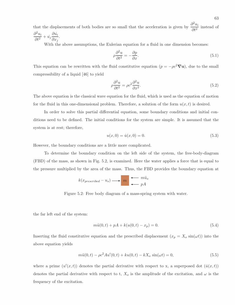
63
that the displacements of both bodies are so small that the acceleration is given by∂2ui∂t2
instead of
∂2ui∂t2
+ uj∂ui∂xj
.
With the above assumptions, the Eulerian equation for a fluid in one dimension becomes:
ρ∂2u
∂t2= −∂p
∂x. (5.1)
This equation can be rewritten with the fluid constitutive equation (p = −ρc2∇u), due to the small
compressibility of a liquid [46] to yield
ρ∂2u
∂t2= ρc2
∂2u
∂x2. (5.2)
The above equation is the classical wave equation for the fluid, which is used as the equation of motion
for the fluid in this one-dimensional problem. Therefore, a solution of the form u(x, t) is desired.
In order to solve this partial differential equation, some boundary conditions and initial con-
ditions need to be defined. The initial conditions for the system are simple. It is assumed that the
system is at rest; therefore,
u(x, 0) = u(x, 0) = 0. (5.3)
However, the boundary conditions are a little more complicated.
To determine the boundary condition on the left side of the system, the free-body-diagram
(FBD) of the mass, as shown in Fig. 5.2, is examined. Here the water applies a force that is equal to
the pressure multiplied by the area of the mass. Thus, the FBD provides the boundary equation at
mus
pAmk(xprescribed − us)
Figure 5.2: Free body diagram of a mass-spring system with water.
the far left end of the system:
mu(0, t) + pA+ k(u(0, t) − xp) = 0. (5.4)
Inserting the fluid constitutive equation and the prescribed displacement (xp = Xo sin(ωt)) into the
above equation yields
mu(0, t) − ρc2Au′(0, t) + ku(0, t) − kXo sin(ωt) = 0, (5.5)
where a prime (u′(x, t)) denotes the partial derivative with respect to x, a superposed dot (u(x, t))
denotes the partial derivative with respect to t, Xo is the amplitude of the excitation, and ω is the
frequency of the excitation.

64
In order to solve the wave equation, another boundary condition is required. To obtain this
boundary condition it is assumed that as the water goes to infinite, the displacement is zero.
limx→∞
u(x, t) = 0. (5.6)
This can be approximated with the plane wave approximation (PWA) [42] at a distance L.
p(L) = ρcu(L, t). (5.7)
Once again, the constitutive equation can be used for the pressure and after some simplification the
following boundary condition is found:
u(L, t) = −cu′(L, t). (5.8)
Therefore, the problem is to solve the partial differential equation,
∂2u
∂t2= c2
∂2u
∂x2, (5.9)
with the conditions
mu(0, t) − ρc2Au′(0, t) + ku(0, t) = kXo sin(ωt), (5.10)
u(L, t) = −cu′(L, t), (5.11)
u(x, 0) = 0, (5.12)
u(x, 0) = 0. (5.13)
To solve the equation, the Laplace transform is taken with respect to (t) of Eq. (5.9) [80].
L
∂2u(x, t)
∂t2
= s2L u(x, t) − su(x, 0) − u(x, 0) = c2L
∂2u(x, t)
∂x2
. (5.14)
Two terms drop out, due to the conditions (5.12) and (5.13). On the right, it is assumed that the
integration and differentiation can be interchanged as:
L
∂2u(x, t)
∂x2
=
∫
∞
0e−st
∂2u
∂x2dt =
∂2
∂x2
∫
∞
0e−stu(x, t)dt =
∂2
∂x2L u(x, t).
(5.15)
Writing U(x, s) = L u(x, t); the following is obtained
s2U(x, s) = c2∂2U(x, s)
∂x2,
or∂2U(x, s)
∂x2− s2
c2U(x, s) = 0. (5.16)
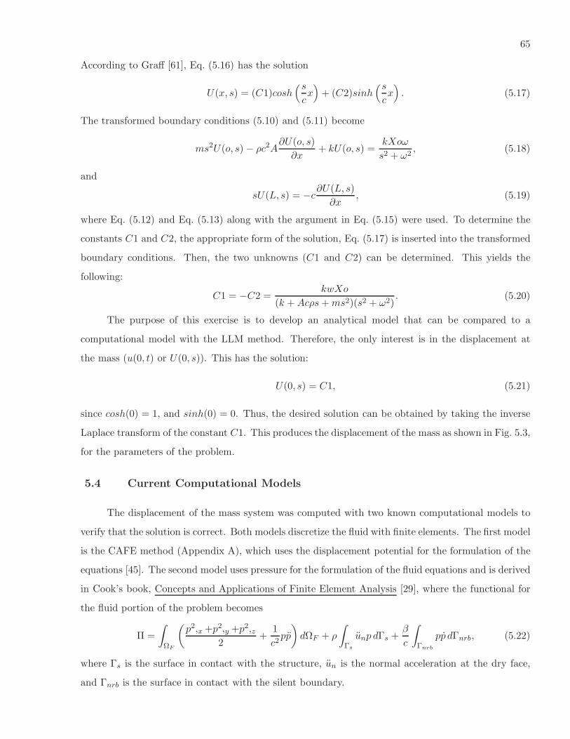
65
According to Graff [61], Eq. (5.16) has the solution
U(x, s) = (C1)cosh(s
cx)
+ (C2)sinh(s
cx)
. (5.17)
The transformed boundary conditions (5.10) and (5.11) become
ms2U(o, s) − ρc2A∂U(o, s)
∂x+ kU(o, s) =
kXoω
s2 + ω2, (5.18)
and
sU(L, s) = −c∂U(L, s)
∂x, (5.19)
where Eq. (5.12) and Eq. (5.13) along with the argument in Eq. (5.15) were used. To determine the
constants C1 and C2, the appropriate form of the solution, Eq. (5.17) is inserted into the transformed
boundary conditions. Then, the two unknowns (C1 and C2) can be determined. This yields the
following:
C1 = −C2 =kwXo
(k +Acρs+ms2)(s2 + ω2). (5.20)
The purpose of this exercise is to develop an analytical model that can be compared to a
computational model with the LLM method. Therefore, the only interest is in the displacement at
the mass (u(0, t) or U(0, s)). This has the solution:
U(0, s) = C1, (5.21)
since cosh(0) = 1, and sinh(0) = 0. Thus, the desired solution can be obtained by taking the inverse
Laplace transform of the constant C1. This produces the displacement of the mass as shown in Fig. 5.3,
for the parameters of the problem.
5.4 Current Computational Models
The displacement of the mass system was computed with two known computational models to
verify that the solution is correct. Both models discretize the fluid with finite elements. The first model
is the CAFE method (Appendix A), which uses the displacement potential for the formulation of the
equations [45]. The second model uses pressure for the formulation of the fluid equations and is derived
in Cook’s book, Concepts and Applications of Finite Element Analysis [29], where the functional for
the fluid portion of the problem becomes
Π =
∫
ΩF
(
p2,x +p2,y +p2,z2
+1
c2pp
)
dΩF + ρ
∫
Γs
unp dΓs +β
c
∫
Γnrb
pp dΓnrb, (5.22)
where Γs is the surface in contact with the structure, un is the normal acceleration at the dry face,
and Γnrb is the surface in contact with the silent boundary.

66
0 5 10 15 20−6
−4
−2
0
2
4
6x 10
−3
Time (s)
Dis
pla
cem
ent
(m)
Figure 5.3: Displacement of the mass in the infinite piston fluid-structure system by an analyticalmethod.
67
Figure 5.4 illustrates that all methods produce the same results; although, this did require that
each method use a prediction step and a time step that met the CFL condition. The blue line in the
figure is the analytical method; the black, dashed colored line is produced by the fluid formulation with
displacement potentials (CAFE); and the red line is produced by the fluid formulation with pressure.
Therefore, this solution will be used to verify the LLM method. In addition, the LLM method will be
compared to the CAFE method.
0 2 4 6 8 10−6
−4
−2
0
2
4
6x 10
−3
AnalyticalCAFEPressure
Time (s)
Dis
pla
cem
ent
(m)
Figure 5.4: Displacement of the mass in the infinite piston fluid-structure system by existing compu-tational models.
5.5 LLM Method Results in 3-D
5.5.1 Matching Meshes Results
The model used for the LLM method is a three dimensional spring, mass, and fluid column as
depicted in Fig. 5.5. This produces the results as shown in Fig. 5.6. As can be seen, the LLM method
produces almost identical results; in fact, the C-error associated with this figure is 0.0007, for a time
step of 0.01 seconds.
5.5.2 Non-matching Results
Given that the matching interface produced such accurate results, it was decided to attempt
non-matching meshes on this problem as well. Therefore, the mass was divided into four elements and
the fluid face was divided into nine elements as depicted in Fig. 5.7. First, the analysis was carried
out with the interface frame discretized as the structure. This also produced no visible errors in the

68
0.1 m
0.1 m
0.1 m
Fluid Silent Boundaryk4 Mass
Figure 5.5: Model with 3-D elements for the LLM method.
0 2 4 6 8 10−6
−4
−2
0
2
4
6x 10
−3
Time (s)
Dis
pla
cem
ent
(m)
LLM MethodAnalytical
Figure 5.6: Comparison between analytical and LLM method with no visible error; C-error = 0.0007.

69
graph, and the C-error was minimal at 0.00062. Then, the same problem was run with the interface
discretized by the zero-moment rule, which produced the interface nodes as depicted in Fig. 5.8. Once
again, the solution produced no visible results and the C-error was negligible at 0.00046. However,
these results are being compared to an analytical solution that was actually solved numerically in
Matlab with the Laplace transform performed in Mathematica.
m
0.1 m
0.1 m
Fluid Silent Boundaryk5 Mass
1
30
Figure 5.7: Model with non-matching meshes.
Therefore, to compare non-matching meshes, it was decided to contrast different meshes with one
that had 100 elements on the faces with a characteristic length of 1100 meters. For a non-matching mesh,
the mass of the structure was created with four elements with a characteristic length of 120 meters. The
fluid was then varied from a characteristic length of 120 to 1
90 . In this analysis, the interface frame was
discretized in the same manner as the structure. This produced the C-error results shown in Fig. 5.9.
At first glance, this looks as if no concrete conclusions can be drawn. However, the characteristic
lengths that appear to have a reduced error actually have the interface nodes at the zero-moment
locations. Coincidentally for these meshes, the zero-moment nodes correspond to the structure nodes.
The other values with a larger error do not meet the zero-moment rule requirement. It is noted that
the zero-moment rule improves the results for this analysis.
In comparing the LLM method with the CAFE method, both produced the same results for this
particular problem. A difference will be noticed in the two dimensional analysis. However, the most
notable item is the time required to run the analysis. The CAFE method requires a much smaller time
step to remain stable. This stability requirement is caused by the prediction step in the method, the
required prediction at the silent boundary, and the system of equations are numerically integrated with
an explicit central difference scheme. By discretizing the fluid into thirty elements and truncating the
fluid at three meters, the time step for the CAFE method was ∆t = 1x10⁻⁶ seconds. In comparison,
by use of the LLM method with an implicit trapezoidal method for the numerical integration, a time
step of ∆t = 1x10⁻¹ seconds was used to produce accurate results. Thus, much fewer time steps
were needed for the LLM method. This more than compensated for the increase in computational

70
Frame nodes
Fluid nodes
Structure nodes
2
45
1
18m
m
Figure 5.8: Interface frame for the non-matching mesh.
10−2
10−1
10−5
10−4
10−3
10−2
Characteristic Length (m)
C-e
rror
Zero Moment Matching
Figure 5.9: C-error for the infinite piston system with non-matching meshes.

71
cost per time step by the LLM method. For instance, by programming both methods in Matlab, the
CAFE method took a little under three hours. The LLM method took nine seconds. Obviously, this
is problem dependent; in some cases, the time step will naturally need to be small to accurately model
the physics.
5.5.3 Stability Verification
Finally, the main point of this chapter was to verify that the partitioned transient method
produced with the LLM method, see Section 3.2, does not have any stability issues if used with an
implicit integration method. Thus, accuracy is imposing the time step rather than stability. Therefore,
an analysis was run with varying time steps. The first time step was taken to be one second, which is
far above the CFL condition for the fluid. The error can visibly be noticed at a time step value of 0.4
seconds. Then, the analysis was run until convergence, which is around 0.01 seconds, see Fig. 5.10.
10−2
10−1
100
10−4
10−3
10−2
10−1
Time step (s)
C-e
rror
Figure 5.10: Time step values and the error associated with the time steps.
5.6 Summary
This chapter provided a problem with an analytical solution of a spring-mass infinite piston. This
was used to verify the ability of the LLM method for a simple fluid-structure interaction. Originally,
this was used to validate the concept of using the gradient matrix; thus, a one-dimensional problem
was studied. The problem was then used to demonstrate the ability of the LLM method with three-
dimensional elements. Given the use of three-dimensional elements, the effect of the zero-moment rule
was shown to be beneficial for non-matching meshes. Finally, the chapter concludes with the fact that
72
the partitioned transient method can be unconditionally stable, if two A-stable integration schemes
are chosen for the fluid and structure models.

Chapter 6
Gravity Dam Benchmark Study: Vibration Analysis
The Koyna dam in India is one of the most famous and studied cases of gravity dams under an
earthquake loading. The majority of the studies involve the non-linear response of the dam, because
during an earthquake in 1967 the dam experienced cracking on its down stream face. However, most
have realized the importance of including the fluid in the simulations. Some of the first work was done
by Zienkiewicz et al. [130] and Chopra et al. [24].
In this chapter, the Koyna dam is also used for FSI to compare different non-matching mesh
techniques. After a short introduction to the problem, this chapter begins with a modal analysis.
This modal analysis provides a good physical understanding of the problem. In addition, kinematic
continuity issues concerned with the discretization of the interface frame are discussed by examining
the mode shapes of the system. This provides some general rules for the discretization of the interface
frame in regards to the method chosen for managing the non-matching meshes. Then, a frequency
content of the acceleration is provided in order to know the dominant frequencies of the earthquake.
The linear vibration portion concludes by investigating a frequency response function of the system.
This illustrates that the LLM method theoretically works for non-matching meshes and gives another
perspective for the physical understanding of the system. The chapter finishes with an example of the
interface patch test to illustrate the benefit of the zero-moment rule, for it assures kinematic continuity
with the LLM method.
6.1 Problem Description
The problem studied in this chapter is a two dimensional dam under seismic excitation. The
dam modeled is the Koyna dam. In December of 1967 an earthquake shook the region and caused
cracking in the down stream direction, see Fig. 6.1. In this study, the dam and the rock foundation
are assumed linear, elastic, isotropic, and homogenous. The dimensions of the dam are shown in
Fig. 6.2 with a coarse mesh. The mesh is truncated at both ends and silent boundaries are applied at

74
those ends. The structures silent boundary was tested by moving the mesh until no visible error was
detected in the results for the dam crest displacement without the fluid. The fluid’s boundary was
discussed in Chapter 4. The parameters for the system are defined in Table 6.1. Several items have
been studied for this problem ranging from crack propagation [67] to the effect of reservoir bottom
absorption [129]. Although, all should be conducted in a true analysis of a gravity dam, in this study
the focus is on the FSI with non-matching meshes.
(a) View of the Koyna dam. (b) Leaks in downstream face.
Figure 6.1: Downstream views of the Koyna dam: (a)Present day. (b) After the earthquake ofDecemeber 1967.
The El Centro earthquake of May 18, 1940, was chosen as the excitation for this problem. The
El Centro earthquake is a low frequency earthquake with a predominant period of 0.55 seconds, see
Fig. 6.3 for the acceleration component in the horizontal direction.
6.2 Linear Vibration Analysis
Before the transient analysis is carried out, a vibration analysis is performed to help determine
the accuracy of the methods. This section begins with a method for deriving the eigenvalue analysis for
the use of Localized Lagrange Multipliers and one for Mortar like methods [8, 13]. The mode shapes
and corresponding frequency are then displayed with the frequency content of the seismic acceleration
so that the relevant modes are determined which will be useful for reduced order modeling. Frequency
Response Functions (FRF) are then examined to give a better physical understanding.
6.2.1 Modal Analysis
An eigenvalue analysis is carried out in a similar manner as that of Park, Felippa, and Ohayon
[99]. Here, it is assumed that the damping and forcing functions are zero for the analysis and that the

75
Dam
Fluid
InterfaceRock Foundation
50 m
0 m
131 m
157 m
Figure 6.2: Koyna dam-reservoir system.
Acc
eler
atio
n(G
)
Time (s)
0
0 5 10 15 20−0.4
−0.3
−0.2
−0.1
0.1
0.2
0.3
Figure 6.3: El Centro earthquake May 18, 1940, horizontal component.

76Econcrete 31.46x10⁹ Pa
ν 0.2ρconcrete 2690 kg/m3
Erock 18x109 Paν 0.2
ρrock 1830 kg/m3
cfluid 1439 m/sρfluid 1019 kg/m3
Table 6.1: Parameters for Koyna dam model.
structural displacements and the fluid displacement potentials are a linear combination of the mode
shapes.
uS = ΦSq, ψ = Φfdϕ, (6.1)
where
[KS − ωSiMS ]ΦSi = 0, [Kfd − ωfdiMfd]Φfdi = 0. (6.2)
Therefore, by replacing the displacement and displacement potential with Eq. (6.1) in the vari-
ational equation set, Eq. (2.55), and pre-multiplying the first two equations by the transpose of the
eigenvector matrices the following is obtained:
ΛS − ω2I 0 ΦTSBS 0 0
0 Λfd − ω2I 0 ΦTfdD
TBF 0
BTSΦS 0 0 0 −LS
0 BTFDΦfd 0 0 −LF
0 0 −LTS −LTF 0
q
ϕ
λS
λF
uB
=
0
0
0
0
0
, (6.3)
where ΛS and Λfd are matrices that contain the particular system’s eigenvalues on the diagonals, and
I is the identity matrix.
Thus, it can be noticed that the combined system’s eigenvectors (Φc) and eigenvalues (Λc) can
be determined from solving:
AcΦc = BcΦcΛc, (6.4)
where
Ac =
ΛS 0 ΦTSBS 0 0
0 Λfd 0 ΦTfdD
TBF 0
BTSΦS 0 0 0 −LS
0 BTFDΦfd 0 0 −LF
0 0 −LTS −LTF 0
; Bc =
I 0 0 0 0
0 I 0 0 0
0 0 0 0 0
0 0 0 0 0
0 0 0 0 0
. (6.5)

77
The eigenvectors (Φc) are currently in modal coordinates and need to be in physical coordinates.
This can be accomplished by the following:
Φ1c = ΦSΦcS (displacement coordinates),
Φ2cd = ΦfdΦcfd (displacement potential coordinates),(6.6)
where ΦcS is the eigenvector portion that is associated with the structure and Φcfd is the eigenvector
portion associated with the fluid. In addition, the system’s eigenvectors that are associated with the
fluid need to be modified from displacement potential coordinates to displacement coordinates. This
can be accomplished by multiplying by the gradient matrix:
Φ2c = DΦ2cd (displacement coordinates). (6.7)
A similar procedure can be carried out to obtain the eigenvalues and eigenvectors if using the
Mortar method, Appendix B. Beginning with the previous derived mode shapes of the subdomains
(ΦS , Φfd), and using Eq. B.2, the following system equation is developed for the Mortar method:
ΛS − ω2I 0 ΦTS BS
0 Λfd − ω2I ΦTfdD
T BF
BTSΦS BT
FDΦfd 0
q
ϕ
λ
=
0
0
0
. (6.8)
Again, the combined system’s eigenvectors (Φc) and eigenvalues (Λc) can be determined from solving:
AcΦc = BcΦcΛc, (6.9)
where
Ac =
ΛS 0 ΦTS BS
0 Λfd ΦTfdD
T BF
BTSΦS BT
FDΦfd 0
; Bc =
I 0 0
0 I 0
0 0 0
. (6.10)
As previously mentioned, the eigenvectors are currently in modal coordinates and would need to be
changed into physical coordinates.
6.2.2 Kinematic Continuity Issues
With the above derivations, the first item to be discussed is kinematic continuity with the
discretization of the interface frame. In order to evaluate the possibilities of non-matching meshes, the
mesh depicted in Fig. 6.4 is examined with the Mortar method and the LLM method. The interface
frame is then discretized as the structure mesh, because this satisfies the zero-moment condition to
pass a consistent stress. A selection of the mode shapes and frequencies for the LLM method are shown

78
0
0
100
100
200
200 300 400 500
50
150
x
y
Figure 6.4: Koyna dam-reservoir system with non-matching meshes
in Fig. 6.5. All of the mode shapes for the LLM method satisfied kinematic continuity at the interface.
Recall that due to the fluid inviscid assumption, only the normal components of the displacements are
constrained at the interface.
On the other hand, the Mortar method with the interface discretized according to the zero-
moment rule exhibits mode shapes where the fluid moves into the structure as illustrated in Fig. 6.6.
It should be noted that this is only caused when the following conditions exist: the interface frame
is discretized with the coarse mesh, the refined mesh is further discretized inside an element of the
coarse mesh, and the Lagrange multipliers shape functions are Dirac delta shape functions that provide
discrete values of the Lagrange multipliers at the nodes.
While the Mortar method produces undesirable results, the LLM method with the Lagrange
multiplier shape functions is not without faults as well. For instance, if the interface frame is discretized
as the refined mesh, and the refined mesh is further discretized inside an element of the coarse mesh,
then a similar problem can be noted for the LLM method, see Fig. 6.7. As discussed in Appendix B,
this formulation of the LLM method produces the same relationship for the boundary displacements
as the Consistent method if the interface frame is discretized as the boundary of the structure and the
structure is more refined then the fluid. Thus, the relevance of using the zero-moment rule is apparent.
Given the above analysis, the following rules need to be applied with discrete Lagrange multipli-
ers collocated at the nodes of the Lagrange boundary. If using the Mortar method, the discretization
of the frame cannot be the coarse mesh. If using the Consistent method, the refined mesh should
always be interpolated to the coarse mesh. This is generally not a problem in aeroelastic problems, for
the fluid is usually much more refined. If using the LLM method, then the interface frame should not
be discretized as the refined mesh. This is actually a positive asset, as using the refined mesh causes

79
(a) 6th mode: 0.54 Hz (b) 20th mode: 1.36 Hz
(c) 21st mode: 2.53 Hz (d) 27th mode: 4.94 Hz
(e) 34th mode: 6.69 Hz (f) 40th mode: 8.13 Hz
(g) 46th mode: 10.1 Hz (h) 49th mode: 11.3 Hz
(i) 55th mode: 12.4 Hz (j) 65th mode: 13.8 Hz
Figure 6.5: Mode frequencies and mode shapes of the system

80
Figure 6.6: 5th Mode shape of the system for the Mortar method with the interface discretized as thecoarse mesh.
Figure 6.7: 30th Mode shape of the system for the LLM method with the interface discretized as therefined mesh.

81
more equations to be solved in the interface equation, Eq. 3.7.
6.2.3 Frequency Content of Acceleration
Given the mode shapes, the frequency content of the acceleration is examined to note which
mode shapes of the system are important. Using the Fast Fourier Transform (FFT), the frequency
contents of the acceleration for the El Centro earthquake are obtained as shown in Fig. 6.8. Thus,
for the horizontal acceleration, the eigenvectors with a frequency up to 8Hz need to be included, and
the vertical acceleration needs the eigenvectors with a frequency up to 15Hz to capture the dominant
shapes. A portion of the dominant mode shapes are shown in Fig. 6.5 for the LLM method.
replacemen
Frequency (Hz)
Pow
ersp
ectr
um
00 10 15 20 25
0.5
1
1.5
2
3
2.5
4
3.5
5
5
4.5
(a) Horizontal accelerationFrequency (Hz)
Pow
ersp
ectr
um
00 10 15 20 255
0.05
0.1
0.15
0.2
0.25
0.3
0.35
0.4
0.45
(b) Vertical acceleration
Figure 6.8: Frequency content of the seismic acceleration.
6.2.4 Frequency Response Function
Next, a selected frequency response function is examined to give a better understanding of the
system. The frequency response plots describe the dynamic response due to a persistent harmonic
excitation with various excitation frequencies [119]. By comparing the vibration amplitude for various
excitation frequencies, the critical vibration frequency for the system can be determined. Here, a
partitioned analysis and an assembled analysis are performed to clarify the dynamic contribution of
each subsystem to the global dynamics.
First, the system is partitioned into two subsystems as was previously done for the LLM method.
Frequency response functions are computed for both subsystems. Figure 6.9 illustrates the frequency
response amplitude of each subsystem in the horizontal (x-direction). The input and output locations
for the frequency response plots are depicted in the top portion of the figure. All response magnitudes

82
are normalized by the static displacement of a unit force at the input degree of freedom (DOF). It
can be noticed that the fluid experiences a zero energy mode when there is no interaction from the
structure. There is only one non-physical zero-energy mode for the fluid when it is partitioned from
the system, which represents the constant displacement potential mode. This is expected, because
this zero-energy mode corresponds to a rigid body mode for the fluid that is formulated in terms of a
displacement potential. This also demonstrates that the fluid formulation only has zero-energy modes
associated with rigid body modes. However, a free surface condition must be applied to remove any
accompanying zero-energy modes with the free surface as noted by Wilson et al. [124].
Input DOF
Output DOF
(a) Input/ output for structure
Input DOF
Output DOF
(b) Input/ output for fluid
Frequency (Hz)
Nor
mal
ized
vib
ration
mag
nitude 103
102
101
100
10−1
10−20 5 10 15 20
(c) Frequency response of the structure
Frequency (Hz)
Nor
mal
ized
vib
ration
mag
nitude 1012
1010
108
106
104
102
100
10−2
10−4
0 5 10 15 20
(d) Frequency response of the fluid
Figure 6.9: Frequency response of the partitioned subsystems.
A couple of items can be noted for the assembled system. First, it is noted that for low frequencies
the system acts as the structure alone, see Fig. 6.10. However, after 3Hz, it is noted that the system
responds to more frequencies than the structure alone, but still responds to the dominate structure
frequencies. Clearly, the assembled system’s response is different than the two systems alone. This
justifies the need for the fluid-structure interaction. Second item to be noted is if the output DOF
is the dam face at the top of the water, and the input DOF is associated with the fluid Lagrange
multiplier at the bottom, then this will produce the same result if the input DOF is associated with
the structure Lagrange multiplier at the same location, as shown in Fig. 6.11. This demonstrates that
the fluid formulation with the LLM method is working. However, if the input DOF stays the same,
such as the one associated with the dam Lagrange multiplier, but the output DOF changes from the

83
structure to the fluid then different results are produced, as shown in Fig. 6.12. This is expected,
because the displacement constraint is that of the normal displacements.
Frequency (Hz)
Nor
mal
ized
vib
ration
mag
nitude 103
102
101
10−1
10−2
100
0 5 10 15 20
Structure AloneAssembled System
(a) Frequency response of the system comparedto the structure.
Frequency (Hz)
Nor
mal
ized
vib
ration
mag
nitude 104
103
102
101
10−1
10−2
10−3
100
0 5 10 15 20
Fluid AloneAssembled System
(b) Frequency response of the system comparedto the fluid.
Figure 6.10: Frequency response of the assembled system.
6.3 Examples of Passing the Patch Test
In this section, an example of the zero-moment rule used to pass the patch test is presented.
The advantage of a simple method used to preserve a constant state of stress is extremely useful. This
has been a recent field of study in contact problems [30, 88]. Crisfield [30] proposed the determination
method of the interpolation function of the contact force field based on the contact patch test, and
demonstrated that an appropriate choice of the function leads to an improvement in accuracy. Here,
Felippa, Park, and Rebel’s [48] work is utilized to maintain an energy-preserving frame. It is on the
frame where the interface equilibrium condition is enforced with the use of the localized Lagrange
multipliers as described in Section 2.3.3.1.
For simplicity, attention is focused on the interface frame with the nodal forces from the subdo-
mains. An example is the interface frame with subdomain forces as shown in Fig. 6.13(b), which is a
characteristic portion of the system with the mesh shown in Fig. 6.13(a). In Fig. 6.13(b), the desired
solution (the bottom forces) is provided, if a uniform stress is applied to the top surface. The top sur-
face constant stress is proportioned to the top nodes by conventional methods, such as node-by-node
lumping.
In this example, six cases are evaluated. The first three consist of the LLM method with
the interface frame discretized as the coarse structure mesh, Fig. 6.14(a); the refined fluid mesh,

84
Frequency (Hz)
Nor
mal
ized
vib
ration
mag
nitude
103
102
101
10−1
10−2
100
0 5 10 15 20
Input DOF = Structure λ
Input DOF = Fluid λ
Figure 6.11: Frequency response of the assembled system with the dam face as the output DOF.
Frequency (Hz)
Nor
mal
ized
vib
ration
mag
nitude
103
102
101
10−1
10−2
10−3
100
0 5 10 15 20
Output DOF = Structure uS
Output DOF = Fluid uF
Figure 6.12: Frequency response of the assembled system with the dam Lagrange multiplier as theinput DOF.
(a) A non-matching mesh for the dam system problem.
0.50.5
1.01.01.0 1.01.0
1.51.5 1.5
0.750.75
∑
f = 6.0
∑
f = 6.0
8
33
(b) A characteristic portion of thenon-matching mesh.
Figure 6.13: An example of a constant state of stress across the interface frame.

85
Fig. 6.14(c); and the use of the zero-moment rule, Fig. 6.14(e). The only discretization that produces
a constant stress state on the bottom is the discretization with the zero-moment rule. Once again, the
LLM method with the coarse mesh, Fig. 6.14(a) is the same as the Consistent Interpolation method,
see Appendix B. Note that with the LLM method, regardless of the interface frame discretization,
the sum of the forces on one side is equal to the other. The next three cases consist of the Mortar
method with the interface frame discretized as the coarse structure mesh, Fig. 6.14(b); the refined
fluid mesh, Fig. 6.14(d); and the use of the zero-moment rule, Fig. 6.14(f). Only the interface with the
coarse mesh, Fig. 6.14(b), has a constant stress on the bottom nodes. However, this interface frame
discretized with the coarse mesh is not conservative, because the sum of the forces on one side is not
equal to the sum of the forces on the other.
These examples are only relevant for the Lagrange multipliers that are interpolated with the use
of the Dirac delta function. However, this provides a very simple, efficient method with the use of the
zero-moment rule that can pass the interface patch test for the LLM method. With the information
from the linear vibration analysis and the zero-moment rule, the next logical step is to begin the
transient analysis.
6.4 Summary
This chapter provided a theoretical understanding of the LLM concept through the exploration
of a frequency response function for the FSI. Also, the linear vibration analysis and the frequency
content of the acceleration provide a physical understanding of the system. It was discovered that the
structure is the dominant subsystem, and would generally require a more refined mesh for a better
representation of the system. If a nonlinear analysis of the structure were performed, then the mesh
would most definitely be more refined than the fluid.
The linear vibration study demonstrated that kinematic continuity problems could develop if
the interface frame was poorly discretized. This produced a set of rules for the discretization of the
interface frame. However, the use of the zero-moment rule for the LLM method will always assure
kinematic continuity at the interface. An example of how the LLM method and the zero-moment rule
are capable of propagating a consistent stress across two domains, an interface patch test, is shown at
the conclusion of this chapter.

86
0.50.5
1.01.01.0 1.01.0
0.830.83
1.33 1.331.66
∑
f = 6.0
∑
f = 6.0
(a) LLM: coarse mesh at interface.
0.50.5
1.01.01.0 1.01.0
0.50.5
1.01.0 1.0
∑
f = 6.0
∑
f = 4.0
(b) Mortar: coarse mesh at interface.
0.50.5
1.01.01.0 1.01.0
0.50.5
2.0 2.01.0
∑
f = 6.0
∑
f = 6.0
(c) LLM: refined mesh at interface.
0.50.5
1.01.01.0 1.01.0
0.830.83
1.33 1.331.66
∑
f = 6.0
∑
f = 6.0
(d) Mortar: refined mesh at interface.
0.50.5
1.01.01.0 1.01.0
1.51.5 1.5
0.750.75
8
33
∑
f = 6.0
∑
f = 6.0
(e) LLM: zero-moment mesh at inter-face.
0.50.5
1.01.01.0 1.01.0
8
3 3
0.610.61
1.77 1.771.22
∑
f = 6.0
∑
f = 6.0
(f) Mortar: zero-moment mesh at in-terface.
Figure 6.14: An example of a constant state of stress across the interface frame, where ”x” is thelocations of the interface nodes.

Chapter 7
Gravity Dam Benchmark Study: Transient Analysis, and Error
7.1 Introduction
This chapter is concerned with the transient response of the Koyna dam subject to the earthquake
loading of the El Centro earthquake in 1940. This chapter begins with a description of the load vector
for the CASE method and the LLM method. Then an analysis with matching meshes is conducted for
both the CASE and the LLM transient methods. Before exploring non-matching meshes, the scaling of
the interface equation for the LLM method is examined with energy errors. Next, an investigation with
non-matching meshes is conducted. For the non-matching meshes, the LLM transient method is first
study. Then the CASE transient method with the inclusion of the LLM for the non-matching meshes
is compared with the CASE transient method with the non-matching handled by the Mortar method.
Once again, it is noted that the LLM method is capable of including the consistent interpolation
method and in locations where it does, it is noted in this chapter.
In this chapter, the acceleration data of the earthquake is amplified by a factor of 1.5. The
seismic excitation is modeled in both the horizontal direction and the vertical direction. It is assumed
that the entire base is excited at the same excitation rate at all nodes at a particular period in time.
Thus, the acceleration, velocity, and displacement are known at the base of the rock foundation at
each given time.
7.2 Load Vector
In many earthquake engineering analyses the load vector is determined from a relative dis-
placement concept [68], given below. In the CASE method the fluid code must receive the total
displacement. In the CASE method this is not a problem, because the total displacement to be sent to
the fluid code can be determined by adding the relative displacement to the given ground displacement.
However, in the LLM method the Interface equation, Eq. (3.7) also needs the total displacement, total
velocity, and the total acceleration. This can also be accomplished by adding the relative displace-

88
ment to the ground displacement and similar for the velocity and the acceleration. However, to avoid
confusion and to create simplicity, it is best to use the total displacement, total velocity, and total
acceleration in the equations. This load vector is described following the relative displacement concept
load vector.
7.2.1 Relative Displacement’s Load Vector
To illustrate the concept, consider the typical dynamic structure shown in Fig. 7.1, where ki
represents the lateral stiffness of a member, mi is the mass of the member, and lateral viscosity is
ignored for clarity. Here, the structure is subject to an earthquake induced displacement, velocity, and
acceleration (ug, ug, ug). Summation of the forces produces the following:
m1u1 − k2(u2 − u1) = 0,
m2u2 + k2(u2 − u1) − k3(u3 − u2) = 0,
m3u3 + k3(u3 − u2) = 0.
(7.1)
k3
2
k3
2
k2
2
k2
2
u3
u2
u1 = ugug
x2
x3
m3m3m3
m2m2m2
m1 m1m1
k3(u3 − u2)
k2(u2 − u1)k3(u3 − u2)
k2(u2 − u1)
m3u3
m2u2
m1u1
FBDRigid Body Motion
Figure 7.1: Relative displacement concept.
A relative displacement is defined as follows given the earthquake displacement (ug) and accel-
eration (ug).
x1 = u1 − ug; thus, x1 = u1 − ug.
x2 = u2 − ug; thus, x2 = u2 − ug.
x3 = u3 − ug; thus, x3 = u3 − ug.
(7.2)

89
Inserting Eq. (7.2) in Eq. (7.1) provides the following equation set in matrix form.
m1 0 0
0 m2 0
0 0 m3
x1
x2
x3
+
k2 −k2 0
−k2 k2 + k3 −k3
0 −k3 k3
x1
x2
x3
= −
m1 0 0
0 m2 0
0 0 m3
ug
ug
ug
. (7.3)
Note the boundary condition x1 = u1 − ug = 0, provides the reduced system
m2 0
0 m3
x2
x3
+
−k2 + k3 −k3
−k3 k3
x2
x3
= −
m2 0
0 m3
ug
ug
. (7.4)
Once again, it is important to remember that the total displacement is the sum of the relative dis-
placement plus the ground displacement. This formulation is used for the CASE method problems.
7.2.2 Total Displacement’s Load Vector
The total displacement’s load vector maintains the equations of motion of the system in terms of
the total state variables. If the structure is redrawn in a more intuitive motion, as shown in Fig. 7.2,
the summation of the forces will still be the same; however, in the below equation, Eq. (7.5), the
displacements have been reversed to reflect the situation in Fig. 7.2.
m1u1 + k2(u1 − u2) = 0.
m2u2 − k2(u1 − u2) + k3(u2 − u3) = 0.
m3u3 − k3(u2 − u3) = 0.
(7.5)
k3
2
k3
2
k2
2
k2
2
u3
u2
u1 = ugug
m3m3 m3
m2m2m2
m1m1m1
k3(u2 − u3)
k2(u1 − u2)
k3(u2 − u3)
k2(u1 − u2)
m3u3
m2u2
m1u1
FBDRigid Body Motion
Figure 7.2: Total displacement concept.

90
This provides the matrix form:
m1 0 0
0 m2 0
0 0 m3
u1
u2
u3
+
k2 −k2 0
−k2 k2 + k3 −k3
0 −k3 k3
u1
u2
u3
=
0
0
0
. (7.6)
Once again, the boundary condition needs to be applied u1 = ug and u1 = ug; thus, a nonzero
prescribed boundary is used. A simple method is to augment the force vector (f) by multiplying
the full mass and stiffness matrices by their respective state variable values with only the prescribed
values:
f = −
m1 0 0
0 m2 0
0 0 m3
u1 = ug
0
0
−
k2 −k2 0
−k2 k2 + k3 −k3
0 −k3 k3
u1 = ug
0
0
. (7.7)
Then, the set of equations associated with the prescribed boundaries are removed to yield the following
system of equations:
m2 0
0 m3
u2
u3
+
−k2 + k3 −k3
−k3 k3
u2
u3
=
k2ug
0
. (7.8)
7.3 Matching Mesh Comparison for CASE/CAFE and LLM
Before evaluating the non-matching capabilities of the proposed method, a set of benchmark
data is established for the matching mesh case for the transient analysis with the CASE and the LLM
methods. In both transient methods, the mesh is refined until convergence is observed for the relative
displacement at the crest of dam. Both methods showed great convergence with the mesh shown
below in Fig. 7.3. The C-error for both methods with varying meshes is shown in Fig. 7.4. Here, the
benchmark mesh contains 3598 DOF for the system. The displacements for both methods are shown
in Fig. 7.5, where they are remarkably similar. Thus, each solution will be used for the benchmark
results for the given method when evaluating non-matching meshes.
7.4 Scaling the Interface Matrix Verification
Before the non-matching analysis is discussed, a brief moment is taken to verify the benefit of
scaling the interface equation, Eq. 3.7, as described in Section 3.2.1. The interface equation has a
potential to be extremely ill-conditioned. The ill-conditioned nature arises because the values of the
interface equation matrix may vary greatly in size, due to the heterogeneous physical systems and
the magnitude of the connection matrices (L). For example, if the standard parameters are used for

91
Figure 7.3: Portion of Koyna dam mesh used as benchmark mesh for C-error.
Total System DOF
C-e
rror
0.1
0.01100 1000 10000
(a) LLM Transient method
Total System DOF
C-e
rror
0.1
0.01
100 1000 10000
(b) CASE Transient method
Figure 7.4: C-error values with matching meshes.
0 1 2 3 4 5 6 7 8−0.2
−0.15
−0.1
−0.05
0
0.05
0.1
0.15
Time (s)
Dis
pla
cem
ent
(m)
CASE
LLM
Figure 7.5: Crest Displacement of Koyna dam of converge results for the transient analysis by theLLM method and the CASE method.

92
the physical components of the system shown in Fig. 6.13(a), then the interface matrix will have a
condition number of 5.9845x10⁶ where the condition number was determined from the spectral norm.
However, if the matrix is scaled as discussed in Section 3.2.1, then the matrix is well conditioned with
a condition number of 38.5592. Clearly, the benefit of scaling is realized.
However, this scaling does introduce a small numerical rounding error. This is noticed by
examining the difference in energy at the interface frame, as discussed in Section 3.4 and written
below for convenience.
W (n)interror = uTB(−LTSλS − LTFλF )
The only contributor to this error is the difference in the Lagrange multipliers at the boundary. This
can be caused by the connection matrices, LS and LF , or the scaling matrices, SF , SS , and SB , used
for the interface equation. If matching meshes are examined, then the only cause of error would be
from the scaling matrices, which is noticed in Fig. 7.6. Here, it is noticed that the difference in energy
is extremely minimal. The maximum absolute value is 3.15x10⁻⁷ Nm when the work on one side of
the interface is equal to 2.2x10⁸ Nm at the maximum value. Thus, it appears that this is caused by
round-off error during the solutions of the systems with the scaling matrices. There is no interface
equation in matching meshes with the CASE transient method; however, the connection matrices LS
and LF are used. Thus, for the matching mesh case, there will be no round-off error and, as expected,
there is no energy difference at the interface. This was noticed for all of the matching meshes run
under the CASE method.
0 1 2 3 4 5 6 7 8−4
−3
−2
−1
0
1
2
3x 10
−7
Time (s)
Ener
gy(Nm
)
Maximum = −3.15x10⁻⁷Nm
Figure 7.6: Energy difference caused by scaling at the interface of matching meshes. Energy on oneside of the interface is of the magnitude of 106 Nm on average.

93
7.5 Non-Matching Mesh Comparisons for both CASE and LLM
In this section, the ability of the localized Lagrange multipliers for non-matching meshes of
different subdomains is evaluated with the transient method developed by the LLM method and
the CASE method. Some general trends will be discussed in regards to the different methods for
non-matching meshes. Before, discussing the pros and cons of each method an example problem is
provided.
As an example, the mesh shown in Fig. 6.13(a) is tested, and provides a discretization for a
portion of the interface as shown in Fig. 6.14. Here, the fluid length is characterized by the height
of the elements in contact with the dam (5.5 m in this problem). The structure length is the height
of elements at the same location (8.25 m in this problem). The interface is then discretized as either
matching the structure mesh, matching the fluid mesh, or by the zero-moment rule. In some other
simulations, the zero-moment rule is the same as the structure or the fluid.
The relative displacement at the crest of the dam is shown in Fig. 7.7 where the transient
method is provided by the LLM concept for this example problem. This figure depicts the three
different results for the different interface frame discretizations. As is typical for the majority of the
simulations, the difference in relative displacement is small. Here, it is noted that the zero-moment
rule does not provide the best results in terms of the C-error. However, it is very close.
0 1 2 3 4 5 6 7 8−0.2
−0.15
−0.1
−0.05
0
0.05
0.1
0.15
Time (s)
Dis
pla
cem
ent
(m)
Zero moment rule (C-error = 0.105)
Refined match (C-error = 0.168)
Coarse match (C-error = 0.104)
Figure 7.7: Dam crest displacement values for different interface meshing with LLM for the transientanalysis and non-matching meshes.
It should be noted that there is a situation in other simulations with the potential to become
problematic. If the interface is discretized as the refined mesh, and the refined mesh is discretized

94
within the coarse mesh, then the forces from the refined mesh inside the coarse mesh are not transferred
to the coarse mesh, this is depicted in Fig. 7.8. This can become a serious issue if it is difficult to
determine which is the refined mesh or if the meshes change from being the refined to the coarse along
the boundary. Fortunately, this can be detected by examining the energy error across the interface
as explained in Section 3.4. If this situation arises, the system will become non-conservative in terms
of energy at the subdomains’ interface boundaries. However, this will be avoided if the zero-moment
rule is used, as it assures that with the LLM method all forces are transferred to the other domain.
In addition, by matching the coarse mesh the forces are correctly transferred.
Fluid Boundary
Interface frame
λF
λS
Structure Boundary
(a) Interface meshmatching the refinedmesh
Fluid Boundary
Interface frame
λF
λS
Structure Boundary
(b) Interface meshmatching the coarsemesh
Figure 7.8: Transfer of forces with the LLM method.
The difference in the energy across the interface frame discretized by the zero-moment rule for the
example problem is shown in Fig. 7.9. The average absolute value of the energy difference is 1.16x10⁻⁷
Nm, which is incredibly insignificant compared to the average energy on the structural boundary at
the interface (6.78x10⁶ Nm). Thus, it is shown that using the localize Lagrange multipliers creates a
conservative system.
The same example problem is used with the CASE transient code with the use of the LLM
method for the non-matching meshes as described in Section 3.3. This provides the relative displace-
ment values as shown in Fig. 7.10. Once again, it is difficult to notice a great variance between the
different techniques for discretizing the interface frame. Also, there can be a serious issue if the frame
is discretized as the refined mesh and the refined mesh is significantly more refined than the coarse
mesh. This can result in a severely ill-conditioned matrix,[
LnS(LnS)T]
, which is to be inverted and
used for the relation between the subdomain’s forces. It is again pointed out that the zero-moment
rule will assure that this will not happen, or the coarse mesh should be used for the interface frame
discretization.
Now, the use of the Mortar method with the CASE transient analysis as explained in Ap-
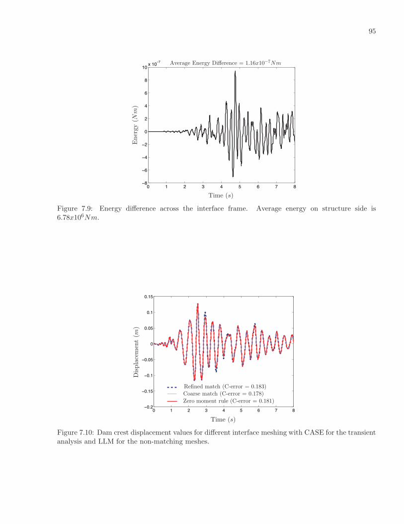
95
0 1 2 3 4 5 6 7 8−8
−6
−4
−2
0
2
4
6
8
10x 10
−7
Time (s)
Ener
gy(Nm
)
Average Energy Difference = 1.16x10⁻⁷Nm
Figure 7.9: Energy difference across the interface frame. Average energy on structure side is6.78x106Nm.
0 1 2 3 4 5 6 7 8−0.2
−0.15
−0.1
−0.05
0
0.05
0.1
0.15
Time (s)
Dis
pla
cem
ent
(m)
Zero moment rule (C-error = 0.181)
Refined match (C-error = 0.183)Coarse match (C-error = 0.178)
Figure 7.10: Dam crest displacement values for different interface meshing with CASE for the transientanalysis and LLM for the non-matching meshes.
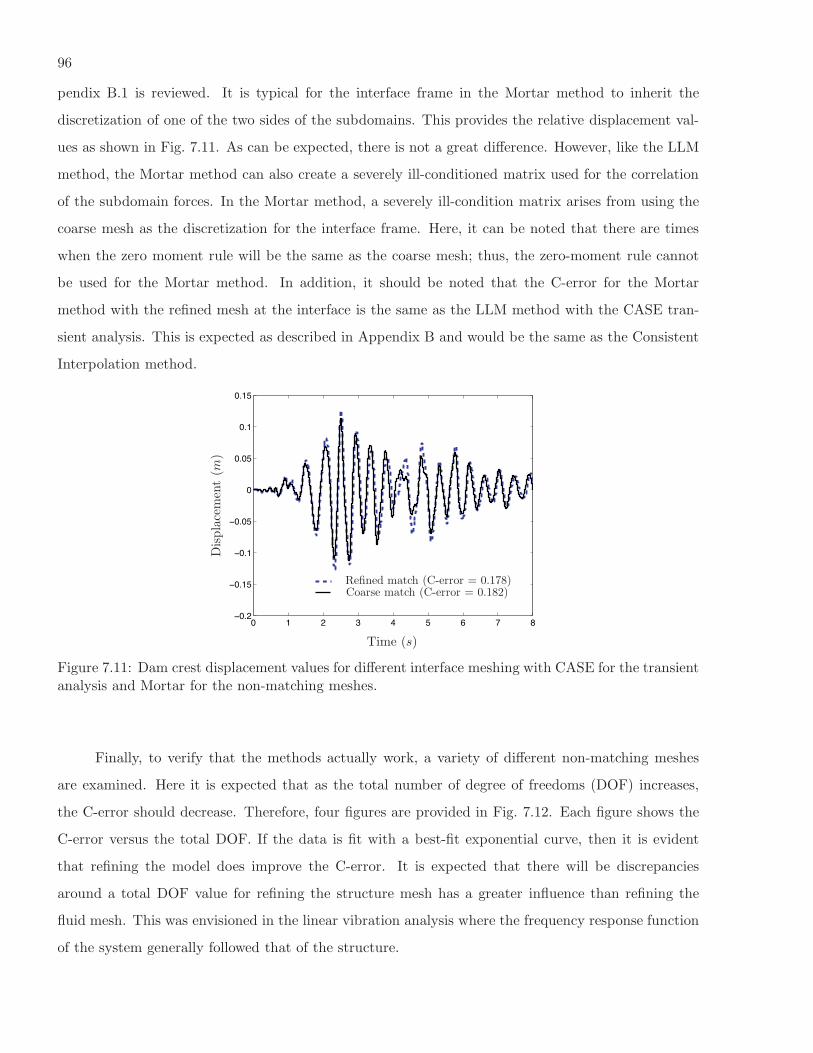
96
pendix B.1 is reviewed. It is typical for the interface frame in the Mortar method to inherit the
discretization of one of the two sides of the subdomains. This provides the relative displacement val-
ues as shown in Fig. 7.11. As can be expected, there is not a great difference. However, like the LLM
method, the Mortar method can also create a severely ill-conditioned matrix used for the correlation
of the subdomain forces. In the Mortar method, a severely ill-condition matrix arises from using the
coarse mesh as the discretization for the interface frame. Here, it can be noted that there are times
when the zero moment rule will be the same as the coarse mesh; thus, the zero-moment rule cannot
be used for the Mortar method. In addition, it should be noted that the C-error for the Mortar
method with the refined mesh at the interface is the same as the LLM method with the CASE tran-
sient analysis. This is expected as described in Appendix B and would be the same as the Consistent
Interpolation method.
0 1 2 3 4 5 6 7 8−0.2
−0.15
−0.1
−0.05
0
0.05
0.1
0.15
Time (s)
Dis
pla
cem
ent
(m)
Refined match (C-error = 0.178)Coarse match (C-error = 0.182)
Figure 7.11: Dam crest displacement values for different interface meshing with CASE for the transientanalysis and Mortar for the non-matching meshes.
Finally, to verify that the methods actually work, a variety of different non-matching meshes
are examined. Here it is expected that as the total number of degree of freedoms (DOF) increases,
the C-error should decrease. Therefore, four figures are provided in Fig. 7.12. Each figure shows the
C-error versus the total DOF. If the data is fit with a best-fit exponential curve, then it is evident
that refining the model does improve the C-error. It is expected that there will be discrepancies
around a total DOF value for refining the structure mesh has a greater influence than refining the
fluid mesh. This was envisioned in the linear vibration analysis where the frequency response function
of the system generally followed that of the structure.
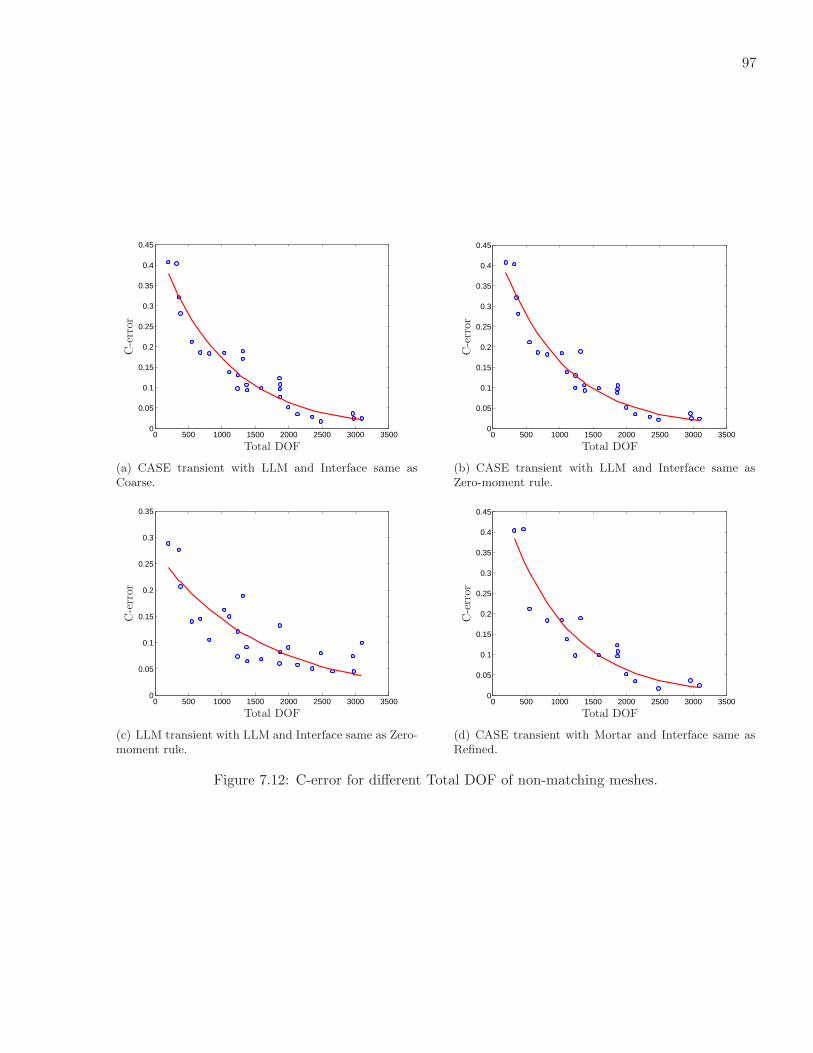
97
0 500 1000 1500 2000 2500 3000 35000
0.05
0.1
0.15
0.2
0.25
0.3
0.35
0.4
0.45
C-e
rror
Total DOF
(a) CASE transient with LLM and Interface same asCoarse.
0 500 1000 1500 2000 2500 3000 35000
0.05
0.1
0.15
0.2
0.25
0.3
0.35
0.4
0.45
C-e
rror
Total DOF
(b) CASE transient with LLM and Interface same asZero-moment rule.
0 500 1000 1500 2000 2500 3000 35000
0.05
0.1
0.15
0.2
0.25
0.3
0.35
C-e
rror
Total DOF
(c) LLM transient with LLM and Interface same as Zero-moment rule.
0 500 1000 1500 2000 2500 3000 35000
0.05
0.1
0.15
0.2
0.25
0.3
0.35
0.4
0.45
C-e
rror
Total DOF
(d) CASE transient with Mortar and Interface same asRefined.
Figure 7.12: C-error for different Total DOF of non-matching meshes.
98
7.6 Summary
The main findings of this chapter pertain to the discretization of the interface frame regardless
of the method used for non-matching meshes. The primary discovery was that if the zero-moment
rule is not used with the LLM method, then there is potential for concerns either with highly ill-
conditioned relation matrices or incredibly non-conservative energy systems. This observation was
first noted during the linear vibration analysis where kinematic continuity issues were examined with
the use of the system’s mode shapes. This was also discussed during the transient analysis for non-
matching meshes. In the transient analysis, the use of the zero-moment rule performed nearly as
well as any other interface discretization; thus, establishing that the zero-moment rule and the LLM
method should be the preferred procedure for non-matching meshes.
During the transient analysis, it is noted that running the LLM method given the implementation
presented in this study with the interface frame discretized as the coarse mesh produces the same results
as the Consistent Interpolation method discussed in Appendix B. Finally, it was also observed that
for problems in this study the structure required a greater refinement then the fluid for convergence.
Therefore, a need for non-matching meshes at the interface is justified.

Chapter 8
Reduced Order Modeling and Cavitation with the Transient LLM method
Any multi-physics system contains several difficult aspects for implementation. This study has
focused on the interaction of the heterogeneous systems. Now, the direction of study takes a slight turn
and looks at reduced order formulations and the nonlinear effect of cavitation for the transient analysis
developed in conjunction with the LLM method. This chapter then concludes with a discussion of
the operational cost of using the LLM transient method versus other explicit, staggered, partitioned
methods.
8.1 Reduced Order Modeling
This section discusses the possibility of using reduced order formulations for the problems in
this study. The objective of any reduced order model (ROM) is to reduce the size of the system; thus,
reducing the number of equations to be solved. For instance, suppose the size of uS and ψ are large
and of order ns and nf respectively. Then, a reduction to the number of degrees of freedom can be
achieved through a set of ks and kf basis vectors:
uS(t) =
ks∑
j
qj(t)φj = ΦSq(t),
ψ(t) =
kf∑
j
ϕj(t)φj = Φfdϕ(t),
(8.1)
where ks and kf are smaller than ns and nf , and ΦS and Φfd are the set of basis vectors. Here it can
be noticed that the fluid has already been reduced from a displacement to a displacement potential,
where the gradient matrix, D, was composed of the basis vectors. Hence, by forcing the irrotational
condition the fluid system is reduced by half.
uF = Dψ.
Therefore, in a similar manner, but including the structural equation, the systems energy func-
tional, Eq. 2.54, is modified. Thus, pre-multiplying the energy functional of the structure by the

100
structure set of basis vectors and doing the equivalent for the fluid, produces the following equation
set:
δΠ(q,ϕ,λS,λF ,uB) =
δqT (ΦTSMSΦSq + ΦT
SCSΦSq + ΦTSKSΦSq + ΦT
SBSλS −ΦTS fS)+
δϕT (ΦTfdMfdΦfdϕ+ ΦT
fdCfdΦfdϕ+ ΦTfdKfdΦfdϕ+ ΦT
fdDTBFλF − ΦT
fdDT fF )+
δλTS (BTSΦSq − LSuB) + δλTF (BT
FDΦfdϕ− LFuB)+
δuTB(−LTSλS − LTFλF ).
(8.2)
Given this reduced equation set the transient analysis can be performed in the same manner as in
Section 3.2.
One of the greatest difficulties in any multi-physics problem is the selection of the basis to use for
the reduction. Allen [1] recommends the use of proper orthogonal decomposition (POD) for coupled
multiphysics problems. Ohayon [95] uses Ritz vectors for situations with FSI, where the Ritz vector
for the fluid is determined by considering the response of the fluid to a prescribed displacement at
the fluid-structure interface. Despite all warnings, the set of basis vectors chosen for this study is the
physical eigenmodes, see Section 6.2.
With the coupled system, it was noticed that there are several low frequency sloshing modes that
have little effect on the structure. Thus, if these were chosen has a basis for reduction, the structure
system equations could potentially become severely ill-conditioned. An alternate method to address
this concern would be to use a reduced basis set for the structure that consists of eigenvectors from the
coupled system that visibly show effect on the structure. However, this can be tedious to determine.
Therefore, each subsystem’s eigenmodes are used for the reduction. However, has Ohayon notes [95]
that if the dry structure modes are used, very slow convergence can be expected. Nonetheless, using
the subsystem’s eigenmodes can demonstrate the ability of the method to incorporate reduced order
modeling.
8.1.1 Computational Results for ROM
In order to evaluate the ability of the LLM method to incorporate reduced order modeling, the
refined non-matching mesh as shown in Fig. 8.1 is used. First, all the eigenvectors of the fluid are used
while the structure’s use of eigenvectors for the basis are being decreased until a substantial error is
noticed. Then, the same procedure is repeated for the fluid. The results are shown in Fig. 8.2, where
the frequency associated with each eigenvector is displayed. As can be seen, the fluid can be reduced

101
to a frequency much closer to the excitation frequency, see Fig. 6.9, where a maximum value of 15Hz
should be considered. The ability of the fluid to be reduced further is expected for a couple of reasons.
First, as already noted, the dam has a greater influence on the system than that of the fluid. Second,
the fluid can include many low frequency modes in the first few sets of modes. Third, using the dry
modes of the structure has demonstrated the need to include more mode shapes, but this does not
limit the ability for this particular problem. However, there is a concern about how quickly the fluid
selection can become inaccurate. Given the above, if the maximum excitation frequency is around
15Hz then the fluid eigenvectors that are associated with two times that amount should be included
and the structure system should include its eigenvectors associated with six times that amount. When
performed in this problem, each system’s equations are reduced to 20% their original value with the
response as shown in Fig. 8.3. Here the response of the ROM is compared to the refined system that
originally showed convergence. It can be noticed that the ROM performs exceptionally well given the
fact that the meshes are non-matching.
Figure 8.1: Characteristic portion of the non-matching mesh used for the ROM test.
There are methods for improvement of the ROM; however, none are present in this portion of
the study so that the potential of the method can be substantiated. It has been demonstrated here
that it can be rather easy to include a reduced formulation for the LLM method. Next, the effect of
a non-linear analysis is examined through the physical concept of cavitation.
8.2 Cavitation
The main benchmark problem of this study is a dam under seismic excitation. During severe
ground motion, it is possible that the absolute water pressure may drop below the water vapor pressure,
producing the phenomenon known as cavitation [5, 85, 113]. The pressure of the water may drop to the

102
0 5 10 15 20 25 30 350.06
0.08
0.1
0.12
0.14
0.16
0.18
0.2
Frequency (Hz)
C-e
rror
(a) Reducing fluids system only.
20 40 60 80 100 120 140 1600.04
0.06
0.08
0.1
0.12
0.14
0.16
0.18
Frequency (Hz)
C-e
rror
(b) Reducing structure system only.
Figure 8.2: Reduction of system up to the frequency of the eigenvector.
0 1 2 3 4 5 6 7 8−0.2
−0.15
−0.1
−0.05
0
0.05
0.1
0.15
Time (s)
Dis
pla
cem
ent
(m)
ROM (C-error = 0.066)Refined matching mesh
Figure 8.3: Dam crest displacement values for a reduced order model using 20% of the eigenvectors ofthe structure and the fluid.

103
water vapor pressure during the period when the dam’s wetface is pulling away from the fluid, which
has been noted in numerous articles and in an experiment by Niwa and Clough [93]. This changes the
hydrodynamic forces on the dam and has the potential to effect the response of the dam. Clough and
Chu-han [27] have noted the possibility that the tensile stress can be increased by 20 − 40% during
the impact of the water against the dam face caused by the closure of the cavitation region. This is a
concern due to the fact that the increased tensile stress may cause crack growth.
When the dam face moves away from the fluid, the absolute water pressure falls below the
vapor pressure causing a micro bubble formulation known has cavitation [105]. In order to model
this phenomenon two models have been presented in the literature. Both models utilize a bilinear
relationship and note that during the process of cavitation the compressibility and the bulk modulus
of the water are reduced towards zero, see Fig. 8.4 [114], where p is the pressure, pv is the vapor
pressure, K is the bulk modulus of the fluid, ρ0 is the density of the saturated liquid, and ρ is
the instantaneous density. Thus, the first model utilizes the fact that the incipience of cavitation is
associated with a local sudden drop in the tangent water compressibility and thus modifies the fluid
stiffness [36, 96]. The second model utilizes the fact that the pressure of the cavitation region has
changed and makes appropriate corrections through the pressure term [45, 109, 114, 130].
p
(ρ − ρ0)/ρ00
Κ
−pv
Figure 8.4: Density pressure relation for a bilinear fluid [114].
The method of including cavitation by modifying the pressure is incredibly convenient, because
it simplifies the analysis. The absolute pressure is either the equilibrium pressure plus pressure de-
termined from the bulk modulus and the volume strain, or it is zero. If the analysis begins in static
equilibrium [130], then
p =
−Kδuiδxi
, if p+ ph > 0,
−ph, otherwise,(8.3)
where it has been assumed that the vapor pressure is negligible in comparison to the atmospheric
pressure (pv = 0), ph is the hydrostatic pressure, and K represents the bulk modulus. In order to
104
utilize this relation, a variable in the fluid equations needs to be related to the pressure term. The
second derivative of the displacement potential is related to the pressure by using Eq. (2.5), Eq. (2.36),
and the wave equation, all written below for convenience.
p = −K∂uFk∂xk
= −ρF c2∂uFk∂xk
.
uF i = ∇ψ.
ψ = c2∇2ψ. (8.4)
Therefore, the second time derivative of the displacement potential is equal to the negative pressure
via the fluid density:
ψ =−pρ. (8.5)
Conveniently, the transient analysis is carried out by solving for the second time derivative of the
state variables. However, it would be an error to adjust this value for the LLM method. In essence,
modifying this second time derivative of the displacement potential modifies the displacement of the
fluid. This then causes conservation of energy concerns at the interface, because the force displacement
relationship on the structure side is not the same as the force displacement relation on the fluid side.
The LLM transient method actually illustrates this problem. This is because the LLM method enforces
the subdomain boundary displacements to be the same and is conservative in an energy sense. If the
above analysis were to be used, then during the time step, the fluid boundary displacement would
be reassigned another value. This causes a greater value for the Lagrange multiplier of the structure,
as it would tend to try and glue the values back together. Ultimately, this could lead to drift of the
structure.
Therefore, the logical implementation of cavitation for the LLM method is to adjust the bulk
modulus of the fluid. By adjusting the bulk modulus, the displacement of the fluid boundary and
the structure boundary maintain their equilibrium values, yet the fluid’s rigidity drastically changes
during cavitation. This method is described in the remainder of this section. Here, the internal energy
can change within an element, but not the overall system energy.
8.2.1 Modification of the Fluid Element Stiffness for Cavitation
Intuitively, the region of cavitation will be characterized by approximately a uniform pressure
that is equal to the pressure of the gas. Mechanically, the region of cavitation experiences a bulk
modulus close to zero, and this condition persists until the pressure is increased again by the collapse
of the cavitated region [36]. A simple but satisfactory model to implement this phenomenon is a

105
bilinear one in which the bulk modulus is that of water, considered as an acoustic medium, when
pressure is superior to the vaporization pressure, and zero when pressure is less then or equal to the
vaporization pressure. The modification of the constitutive properties during cavitation is similar to
crack smearing approaches for tensile crack growth in concrete [19, 73].
To incorporate this bilinear behavior, the pressure must be calculated at each time step. Due to
the assumption of the small compressibility of a liquid, the pressure can be calculated from Eq. (2.5).
This leads to the pressure being determined by the volumetric strain displacement matrix as done in
Section 4.3. Therefore, the pressure is found at gauss points for full integration. Given these values,
the element pressure is determined at the center, as computed stresses are usually most accurate at
locations within an element rather than on its boundaries [29].
Another method for computing the pressure in the element is to compute the pressure at the
nodes, p, due to the following relation.
p = −ρψ, (8.6)
which was derived from above, Eq. (8.5). Given the pressure at the nodes, the element pressure can
be assumed to be the average of the node pressures. This appears to be more convenient, because the
displacement volume strain matrix does not need to be stored. In addition, this would remove the
error associated with determining the fluid displacement from the displacement potential (uF = Dψ).
Regardless of the method chosen for determining the pressure, caution must be taken, as this is the
dynamic pressure if the fluid structure system is initially in static equilibrium. The total pressure
would be the dynamic pressure plus the hydrostatic pressure.
When the total pressure in the element drops below the vapor pressure, then the stiffness matrix
is modified to suppress rigidity for the element. If the total pressure of the element is found to be
less than the vapor pressure, then the stiffness matrix can be modified by assembling the element
stiffness matrix calculated as before, but negative. However, to reduce computational cost during each
time step, it is best to determine the cavitation effect of each element on the matrix Kfd during the
preprocessing phase. Then, if the element is found to be in a cavitation region, the matrix Kfd can
be modified appropriately.
In addition, if cavitation analysis is to be performed it is best to use the Central Difference
form of the Newmark family methods (β = 0, γ = 12). Using the Central Difference is best for two
reasons. First, for an accurate account of cavitation, a small enough time step is needed to assure that
a pressure wave does not move through an element. Since the CFL condition is already being met, it
is better to use an accurate method for small time steps such as the Central Difference method. The
second advantage is due to the computational cost. Using the transient analysis from Section 3.2, the

106
matrix to be inverted is the following for the fluid:
FF =[
Mfd + ∆tγCfd + ∆t2βKfd
]
−1. (8.7)
This matrix is used several times for the determination of the Interface equation, Eq. (3.7), and during
the transient analysis. Thus, it is originally factored with an LU factorization [75], for computational
efficiency during reuse. Therefore, it would be beneficial if this matrix could be factored only once
and reused. Hence, by modifying the stiffness to account for cavitation, the Central Difference method
allows for the matrix FF to only be factored once, for β = 0.
An algorithm to be used during transient analysis is as follows:
(1) Given the forcing values (fn+1S , fn+1
F ), and the previous state variables of the domains (unS ,
unS , unS , ψn, ψ
n, ψ
n) solve the Interface equation, Eq. (3.7), for the Lagrange multipliers
(λn+1S , λn+1
S ).
BTSFSBS 0 LS
0 BTFDFFDTBF LF
LTS LTF 0
λn+1S
λn+1F
un+1B
=
BTSFSg
n+1S
BTFDFFgn+1
F
0
(2) Insert the Lagrange multipliers (λn+1S , λn+1
S ) into Eq. (3.2) and Eq. (3.3), and solve for un+1S
and ψn+1
un+1S = FS(gn+1
S − BSλn+1S ),
ψn+1
= FF (gn+1F − DTBFλ
n+1F ).
(3) Update the values of un+1S , un+1
S , ψn+1, and ψn+1
, with the Eq. (3.1).
(4) Determine the fluid element pressure, pe by either Eq. (4.2) or Eq. (8.6).
(5) Assuming the analysis begins in static equilibrium, check if the element is in the cavitation
region and adjust the matrix Kfd appropriately.
(6) Repeat for the next time step, given the modified matrix Kfd.
8.2.2 Frothing: Spurious Oscillations
After the cavitation region has formed it is possible that the earthquake direction may change.
This causes the micro bubbles region created by cavitation to collapse and and the cavitation region
closes up again. As a result of the sudden closure of the fluid cavities, an impact on the dam will occur

107
[96]. This impact phenomena results in a sharp increase in compressive pressure followed by spurious
oscillations (frothing) [36]. To eliminate these high frequency oscillations several authors [45, 109, 114]
have added a small amount of numerical damping. Others, [36, 96], have added a small amount of
damping to the water domain in their analysis. The small amount of damping required to remove the
frothing has been noted to have a small effect on the response of the system [96].
Given the fluid formulation for the LLM method, it would be easier to implement a modest
amount of damping into the fluid-domain by creating a fluid-damping matrix. This is also conve-
nient because a fluid damping matrix is created for the inclusion of the silent boundaries. El-Aidi
[36] recommended a 0.1 % stiffness-proportional damping in the fundamental pressure mode of the
fluid element. Oskouei [96] recommends a 5.0 % mass-proportional damping plus a variable stiffness
proportional damping. In this study, a classical damping matrix is proposed by the Rayleigh model:
CFd = αKKFd + αMMFd, (8.8)
where the coefficients are determined by the first nonzero frequency values. A damping ratio of 0%
is used for the Mass term and a value of 0.1% is the beginning point for the Stiffness term. The
Stiffness term’s damping ratio is adjusted as appropriate. The Stiffness proportional damping is used
to remove the high frequency oscillations caused by frothing. The mass-proportional term has been
omitted because it would provide some artificial numerical stability during the time-marching process
[73].
8.2.3 Bleich-Sandler Plate Problem
The Bleich Sander plate problem [14] is used to validate the cavitation method for the LLM
method. This benchmark problem has the only known analytical solution for a cavitation problem.
The study is made up of a semi-infinite column of fluid with a constant section that supports a
mass. Gravity and atmospheric pressure are included for this study. An exponential pressure wave
propagates thru the fluid, see Fig. 8.5. The reflection of this wave on the mass creates cavitation.
The fluid is described by 100 elements with the properties given in Table 8.1. Numerical damping
is necessary to suppress frothing with the coefficient of αK = 10−5 and αM = 0 in Eq. (8.8). The
results provided in the following section demonstrate the accuracy of the LLM method.
8.2.3.1 Numerical Solution
In Fig. 8.6, the numerical solution produced by the LLM method is compared to the analytical
solution of this problem given by Bleich and Sandler [14]. The small differences are due, according to

108
x
D
W
g
Plane-Wave Boundary
Exponential
Pressure Wave
patm
Pinc = P0e
“
t+(x−x0)/τ
t
”
H(
t+(x−x0)/τt
)
Figure 8.5: Schematic model of the Bleich-Sandler plate problem.

109ρF 989 kg/m3
c 1451 m/sPatm 0.101 MPag 9.81 m/s2
D 3.81 mW 144.7 kg/m2
P0 0.710 MPaτ 0.996 ms
Table 8.1: Parameters for the Bleich-Sandler plate problem
Sprague and Geers [113], to the use of the plane wave approximation which is not perfect for the whole
range of frequencies, and to the simplicity of the elements as they do not allow perfect propagation.
To solve this problem, Sprague and Geers propose the use of high order elements.
8.2.4 Cavitation in Koyna Dam Analysis
In this section, the reservoir cavitation effects caused by the El Centro earthquake response of
the Koyna dam are investigated. In order to truly consider the effects of cavitation, the El Centro
earthquake response is first amplified so that the maximum magnitude is of the order of 1 g and then
again to 1.5 g in the horizontal direction. The mesh of the system for this analysis is shown in Fig. 8.7,
because of its low C-error in the linear analysis for both the CASE transient analysis (C-error = 0.04)
and the LLM transient analysis (C-error = 0.06). In both methods, frothing is suppressed. The
CASE transient method uses an artificial damping coefficient, β = 0.25 and the LLM method uses a
stiffness proportional damping term with a Rayleigh damping ratio of 0.1%. The LLM method with
the zero-moment rule is used for the non-matching meshes in both transient analyses.
A comparison of the relative displacement of the crest of the dam for the LLM transient method
and the CASE transient method is shown in Fig. 8.8. The cavitation zone is shown for the LLM
transient method in Fig. 8.9. This is has expected with the cavitation being near the surface of the
water and primarily next to the dam’s face, which is on the right side of the figures. In these figures,
frothing has been suppressed. If the minor amount of damping is not added to the fluid domain then
spurious oscillations can be noticed away from the face of the dam as shown in Fig. 8.10.
An interesting observation is that including the effect of cavitation reduces the relative displace-
ment. This observation has been noted by several authors that have examined the effect of cavitation
[36, 27, 96, 49]. Zienkiewicz [130] notes a similar response for the majority of the cases studied in
that article. However, the Koyna dam example does show a spike in the relative displacement after
the major acceleration component of the El Centro earthquake has passed for a second. It is believed

110
Time (s)
Mas
sM
otio
n(m/s
) Bleich & SandlerLLM method
Cavitation Results
Without Cavitation
0
0 0.002 0.004 0.006 0.008 0.01 0.012 0.014 0.016
-0.1
-0.2
0.1
0.2
0.3
0.4
0.5
0.6
0.7
0.8
(a) Velocity response for the mass
Time (s)
Xlo
cation
(m)
Bleich & SandlerLLM method
Closure Point
0.002 0.004 0.008 0.01 0.012 0.014
1
2
3
(b) Cavitation zone
Figure 8.6: Bleich-Sandler plate problem results
Figure 8.7: Koyna dam mesh used for cavitation analysis.
0 2 4 6 8−0.4
−0.3
−0.2
−0.1
0
0.1
0.2
0.3
Time (s)
Dis
pla
cem
ent
(m)
Cavitation ResultsWithout Cavitation
(a) CASE transient method.
0 1 2 3 4 5 6 7 8−0.4
−0.3
−0.2
−0.1
0
0.1
0.2
0.3
Time (s)
Dis
pla
cem
ent
(m)
Cavitation Results
Without Cavitation
(b) LLM transient method.
Figure 8.8: The effects of cavitation on the relative displacement of the dam crest.

111
(a) 1 second (b) 2 seconds
(c) 3 seconds (d) 4 seconds
(e) 5 seconds (f) 6 seconds
(g) 7 seconds (h) 8 seconds
Figure 8.9: Cavitation zone during selective time intervals with the Dam’s face on the right side.
(a) 5 seconds (b) 6 seconds
Figure 8.10: Cavitation zone during selective time intervals with the Dam’s face on the right sidewithout suppressing frothing.

112
that this spike is caused by the spurious oscillations [36], as Zienkiewicz did not try to preclude the
effects of frothing. Zienkiewicz does note that the effect of cavitation is not serious, as found by the
previous authors cited.
Niwa and Clough, [93] performed experimental results with an attempt to include cavitation.
The dam model was separated from the water by a plastic membrane. Since air could access the
dam-membrane interface, separation (i.e. cavitation) occurred whenever the absolute water pressure
was less then the atmospheric pressure. In their results, the authors concluded that in low intensity
accelerations (0.156g) cavitation would have little effect. However, they believe that at high intensity
accelerations (1.21g) cavitation can have a serious effect during the impact action. However, they did
not run tests attempting to suppress the cavitation for comparison. In all fairness, it would be very
difficult to truly model cavitation, and then turning it off would be nearly impossible. In addition, the
scaled model, about 1/150 the actual size, does not attempt to scale the hydrostatic pressure at the
locations of cavitation. Therefore, this study presents cavitation results for the relative displacement
with a maximum acceleration value of 1.5g shown in Fig. 8.11. It is possible that the effect of the
impact is not felt with the acceleration provided in the positive x-direction; therefore, the magnitude
is changed to the other direction and the relative displacement results are shown in Fig. 8.12. In both
cases, including the effect of cavitation actually appeared to reduce the relative displacements. Hence,
as concluded by many [36, 27, 96, 49, 130], the effect of cavitation is minimal and not a necessity for
problems of this nature.
0 2 4 6 8−0.4
−0.3
−0.2
−0.1
0
0.1
0.2
0.3
0.4
0.5
Time (s)
Dis
pla
cem
ent
(m)
Cavitation ResultsWithout Cavitation
Figure 8.11: The effects of cavitation on the relative displacement of the dam crest with the maximumacceleration equal to 1.5g.
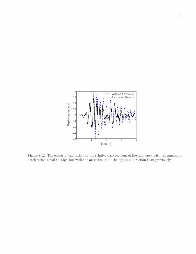
113
0 2 4 6 8−0.4
−0.3
−0.2
−0.1
0
0.1
0.2
0.3
0.4
Time (s)
Dis
pla
cem
ent
(m)
Cavitation ResultsWithout Cavitation
Figure 8.12: The effects of cavitation on the relative displacement of the dam crest with the maximumacceleration equal to 1.5g, but with the acceleration in the opposite direction than previously.

114
8.3 Operational Count
Up to this point, it has been mentioned but not demonstrated that there is additional com-
putational cost of using the LLM transient method versus any other partitioned method with the
non-matching meshes handled by a basic relation matrix. In the LLM method the additional cost is
realized during the solution of the interface equation at each time step; whereas, other partitioned
methods would be using matrix multiplication for transferring loads from one subdomain’s mesh to
another.
It is assumed that the interface equation matrix, Eq. 3.7, has been factored with an LU fac-
torization. This upfront cost would be similar to the cost of creating the relation matrices for the
other methods. Also assume that the interface frame is discretized with the same amount of degree
of freedoms as the refined mesh boundary, say the structure ns. The fluid boundary has nf degrees
of freedom. According to Kincaid, [75], the long operations (multiplication) cost of solving a matrix
equation with an LU factorization for m time steps is
cost =
(
1
2+ml
)
(ne)2, (8.9)
where ne is the number of equations. Therefore, the cost for the interface equation is
costllm =
(
1
2+ml
)
(2ns + nf )2, (8.10)
where ml is the number of time steps for the LLM method. The long operations cost for using a
relation matrix during each time step would be
costmatrix = me(2nsnf ), (8.11)
where me is the number of time steps for this other method. Here there are two instances in which
matrix vector multiplication needs to happen, once for the displacement relation and once for the
force relation. If cavitation is not included, then the LLM transient method can use implicit time
integration schemes where the time step is dictated by accuracy. Assuming that other staggered
partitioned integration procedures use an explicit time integration method with me time steps, the
logical question is, when is it better to use the LLM method (i.e. when are there less operations)?
costllm ≤ costmatrix.
ml(4n2s + 4nsnf + n2
f ) +
(
2n2s + 2nsnf +
1
2n2f
)
≤ 2menfns.
ml ≤2menfns
4n2s + 4nsnf + n2
f
− 1
2.
(8.12)

115
As a worse case scenario, it can be assumed that the number of degrees of freedoms of the two
subdomains are the same, then the number of steps for the LLM transient method should be less than2
9the time steps of the explicit staggered partitioned procedure.
ml ≤2
9me − 1. (8.13)
8.4 Summary
The main point of this chapter is to examine the abilities of the LLM transient method and the
LLM method for non-matching meshes with popular concepts currently being explored for computa-
tional modeling. First, reduced ordering modeling (ROM) was demonstrated for the LLM transient
method with non-matching meshes and a basis chosen as the eigenvectors from the subsystems. Here,
it was noted that a substantial reduction could be accomplished. Next, a non-linear effect of cav-
itation was considered, where it was noted that the effect of including cavitation was small and a
conservative approach to dam analysis would not need to include this effect. Nonetheless, including
cavitation had no effect on the ability of the LLM method for non-matching meshes. However, using
the LLM transient method to include cavitation increased the computational cost as compared to the
CASE transient method, because of the need to use the explicit Central Difference time integration
method in the LLM transient code. Thus, a long operational cost analysis was conducted, and it was
determined that if the number of LLM transient time steps were less than2
9the number of time steps
of any partitioned method, then it was beneficial to use the LLM transient method.

Chapter 9
Partitioned 3-D Problem with Curved Surface
The main purpose of this chapter is to evaluate the LLM method for non-matching meshes on
a curved surface and the implementation of the zero-moment rule on such a surface. The effect of
mapping the interface nodes on the curved surface and the creation of the connection matrices are
explored. A benchmark problem that has a curved surface is the Morrow Point arch dam, which has
been extensively studied in the literature [35, 52, 87, 84, 94, 115, 123].
9.1 Problem Description
The problem studied in this chapter is the Morrow Point dam located on the Gunnison River
in southwest Colorado. The river is confined to a narrow channel cut deep in the rock-walled canyon.
The general geometry is shown in Fig. 9.1. The dam has a height of 142m and a crest length of 219m.
A detailed description of the dam is available from the U.S. Department of the Interior [76]. This arch
dam is generally studied in literature, because of its nearly symmetrical design. Thus, the majority of
the studies take advantage of the symmetry and only model half the dam.
Fok et al. [52] was one of the first to demonstrate the significance of including the effect of the
fluid, the rock foundation, and bottom absorption. Many studies have been conducted to determine
the influence of the surrounding rock at the dam [115, 52, 94, 35]. Tan et al. [115] illustrate that
modeling the rock foundation with the same stiffness as the dam has little effect compared to modeling
the rock foundation as a rigid foundation. However, decreasing the stiffness of the rock by one-forth
the amount of the stiffness of the dam appeared to have significant effects. In this study, the rock
foundation is rigid for comparison purposes with the literature, because the effect of the foundation
has provided varying results. This also provides a better evaluation of the interface condition.
Another controversial topic is the application of the ground motion. It is possible to define the
earthquake input as a rigid-body translation of the basement rock on which the finite element model
of the dam and foundation are supported, as was done for the gravity dam analysis in the previous two

117
(a) View of the Morrow Point dam.
142 m
219 m
(b) Morrow Point dam Geometry. [123]
Figure 9.1: Morrow Point dam representation.

118
chapters. However, there is little data about earthquake motion at a depth from the surface, because
most of the available strong motion records are from accelerometers located at the ground surface [52].
In addition, when truncating the rock foundation to a finite extent, some have applied the motion
to the side of the truncation where others have not. Tan et al. [115] assume the foundation rock is
massless for the dynamic analysis, and the earthquake input is specified as spatially-uniform motion of
the basement rock. Since there is no wave propagation mechanism in the massless foundation rock, the
specified base rock motion is transmitted without modification to the dam-foundation rock interface
[52]. Conveniently, this concern is alleviated with the assumption of a rigid foundation. Thus, the
ground motion is uniformly specified at the dam portions in contact with the rock foundation.
The excitation for this problem is the Taft earthquake of July 21, 1952, recorded at the Lincoln
School Tunnel. In this problem, the greatest acceleration data is applied in the downstream direction
and the other two in the vertical and cross stream directions. The downstream acceleration is shown
in Fig. 9.2 along with its frequency content.
0 5 10 15 20−1.5
−1
−0.5
0
0.5
1
1.5
2
Acc
eler
atio
n(m/s
2)
Time (s)
(a) Acceleration
0 5 10 15 20 250
0.5
1
1.5
2
2.5
Frequency (Hz)
Pow
ersp
ectr
um
(b) Frequency content
Figure 9.2: Ground motion and frequency content of the seismic acceleration recorded at the 1952Taft Lincoln School Tunnel, California earthquake.
A model of the dam and the rigid foundation used for this problem is shown in Fig. 9.3. The
parameters for this problem are defined in Table 9.1.
9.2 Creation of the Connection Matrices
One of the difficult aspects of the LLM method is creating the connection matrices, Lk, where k
is one of the subdomains, the structure or the fluid in this study. This is obviously compounded when
the interface surface is not a normal shape. An atypical shape is the curved surface of the arch dam.
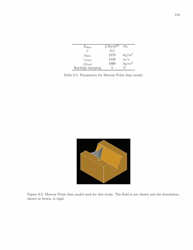
119
Edam 2.76x10¹⁰ Paν 0.2
ρdam 2478 kg/m3
cfluid 1440 m/sρfluid 1000 kg/m3
Rayleigh damping 5 %
Table 9.1: Parameters for Morrow Point dam model.
Figure 9.3: Morrow Point dam model used for this study. The fluid is not shown and the foundation,shown in brown, is rigid.

120
This section provides a simple method for creating these matrices on such a surface. Recall that the
connection matrices are used to relate the interface displacements to the two subdomains’ interface
displacements.
ΠB = λTS (BTSuS − LSuB) + λTF (BT
FuF − LFuB).
The first task is to create the interface nodes. The simplest case is to use the trace of the
discretization of either the structure or fluid subdomain at the interface. However, the zero-moment
rule assures that a conservative system is created and no matrices will be ill-conditioned; thus, it
is discussed. If the surface is fairly regular and not disjointed, then the subdomains’ nodes can be
mapped to a surface element as shown in Fig. 9.4. With the subdomains’ nodes mapped to an interface
η
ξ
(a) Structure
η
ξ
(b) Fluid Domain
Figure 9.4: Mapping of the subdomains nodes to an interface element for use in the zero-moment rule.
element, then the zero-moment rule can be used to determine the discretization of the interface as
shown in Fig. 9.5. The zero-moment rule is used in one-dimension, along one of the mapped element’s
natural coordinates, to determine the node location along the axis. Then, the process is repeated
along the other mapped natural coordinate axis.
Given the following discretization on the mapped interface element, the connection matrices can
be easily created from simplifying the integrations on this mapped interface element. The simplification
can take place because of the use of Dirac delta shape functions for the Lagrange multipliers. For
instances, the connection matrix for the structure, LS, is created as follows:
(1) The process would be to loop through each created boundary frame element.
(2) The normal vector for each boundary frame element is found by mapping the boundary frame
element coordinates back to the physical coordinates of the system. An alternative is to
determine the normal vector of each structure node and use this value.

121
η
ξ
Figure 9.5: Interface nodes ”x” determined by the zero-moment rule.

122
(3) In each boundary frame element, the location of any structure nodes within the element is
determined.
(4) Given the mapped coordinates of the boundary frame’s nodes and the mapped coordinates of
the structure nodes, the natural coordinates of a structure node within the frame element is
deduced.
(5) Knowing the natural coordinates within a boundary frame element of a structure node, the
shape functions of the boundary frame element provide a relation between the nodes of the
frame element and the structure node.
(6) This relationship in conjunction with the normal vector provide the necessary portion of the
connection matrix for the boundary element nodes and the structure node.
This is possible, because of the use of collocated Lagrange multipliers with Dirac delta shape functions.
If linear shape functions were used instead, then the connection matrices would be difficult to form
given the need for piecewise polynomial integration.
9.3 Non-matching Mesh Results
Non-matching meshes for the fluid domain and the structure domain are used for the Morrow
Point arch dam to test the effect of creating the connection matrices as described in the previous
section. First, matching meshes were used until convergence was obtained with the mesh for the dam
as shown in Fig. 9.6. The relative displacement at the crest of the dam in the center of the arch is
used for comparison purposes. The results of the relative displacements are comparable with published
results. There are some minor differences, but these are attributed to the fact that the dam and the
fluid models are slightly different then published models.
Given the results for the converged model, the fluid is then changed so that there are non-
matching meshes at the interface. Figure 9.7 illustrates four different results, where the number
of fluid nodes at the interface is used to indicate the difference in the non-matching meshes. The
structure has 63 nodes at the interface, and the fluid ranges from 42 to 108 nodes at the interface.
The maximum difference between the matched simulation and the non-matched simulation for the
time span is presented in Fig. 9.7. In addition, the C-error for the non-matched mesh compared to
the matched mesh is provided. As can be seen, there is very little difference between the two results;
with the maximum difference, being noted when the meshes are further apart. It is also interesting
to note that the overall relative magnitude is less for the non-matching meshes with the fluid as the
coarse mesh than when the fluid is more refined than the structure.

123
Figure 9.6: Structure Mesh that showed Convergence.
0 5 10 15−0.06
−0.04
−0.02
0
0.02
0.04
0.06
Time (s)
Dis
pla
cem
ent
(m)
Non-matchingMatching
Maximum Difference = 0.005 m at 6.77 sec.
C-error = 0.079M-error = −0.073P-error = 0.029
(a) 42 Fluid Interface Nodes
0 5 10 15−0.06
−0.04
−0.02
0
0.02
0.04
0.06
Time (s)
Dis
pla
cem
ent
(m)
Non-matchingMatching
Maximum Difference = 0.005 m at 6.75 sec.
C-error = 0.079M-error = −0.076P-error = 0.022
(b) 48 Fluid Interface Nodes
0 5 10 15−0.06
−0.04
−0.02
0
0.02
0.04
0.06
Time (s)
Dis
pla
cem
ent
(m)
Non-matchingMatching
Maximum Difference = 0.004 m at 7.1 sec.
C-error = 0.048M-error = 0.036P-error = 0.031
(c) 88 Fluid Interface Nodes
0 5 10 15−0.06
−0.04
−0.02
0
0.02
0.04
0.06
Time (s)
Dis
pla
cem
ent
(m)
Non-matchingMatching
Maximum Difference = 0.010 m at 7.1 sec.
C-error = 0.083M-error = −0.027P-error = 0.078
(d) 108 Fluid Interface Nodes
Figure 9.7: Relative displacement comparison for non-matching mesh versus matched mesh with 63structure interface nodes.
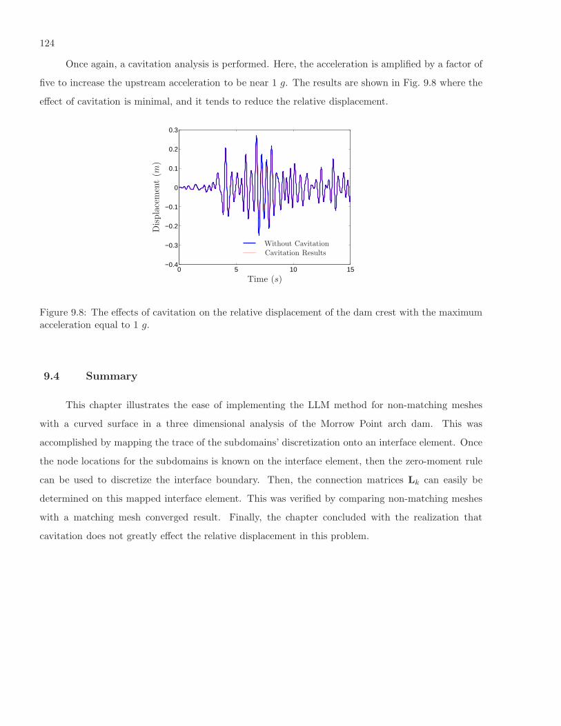
124
Once again, a cavitation analysis is performed. Here, the acceleration is amplified by a factor of
five to increase the upstream acceleration to be near 1 g. The results are shown in Fig. 9.8 where the
effect of cavitation is minimal, and it tends to reduce the relative displacement.
0 5 10 15−0.4
−0.3
−0.2
−0.1
0
0.1
0.2
0.3
Time (s)
Dis
pla
cem
ent
(m)
Cavitation ResultsWithout Cavitation
Figure 9.8: The effects of cavitation on the relative displacement of the dam crest with the maximumacceleration equal to 1 g.
9.4 Summary
This chapter illustrates the ease of implementing the LLM method for non-matching meshes
with a curved surface in a three dimensional analysis of the Morrow Point arch dam. This was
accomplished by mapping the trace of the subdomains’ discretization onto an interface element. Once
the node locations for the subdomains is known on the interface element, then the zero-moment rule
can be used to discretize the interface boundary. Then, the connection matrices Lk can easily be
determined on this mapped interface element. This was verified by comparing non-matching meshes
with a matching mesh converged result. Finally, the chapter concluded with the realization that
cavitation does not greatly effect the relative displacement in this problem.

Chapter 10
Conclusion
This thesis developed an acoustic fluid-structure interaction methodology with Localized La-
grange Multipliers (LLM) used for the coupling of the heterogeneous systems: the emphasis was on
the treatment of non-matching meshes. Beginning with a variational energy formulation, an efficient
partitioned transient analysis was developed, where all the benefits of a partitioned method are re-
alized. This transient analysis is advantageous, because it does not require a prediction step in the
algorithm, which can greatly effect the stability of the any transient method. With the coupling
of the systems performed by LLM, non-matching meshes at the interface are easily managed. The
salient feature of the coupling with LLM is also used to create coupling matrices that can be used in
other acoustic FSI codes. Even with the use of discrete Lagrange multipliers, convergence has been
demonstrated analytically and experimentally for non-matching meshes.
A new fluid formulation was needed in order to exploit the transient analysis that has been de-
veloped. The formulation is carried out by first employing a fluid displacement formulation to assure
an energy form. The displacement potential formulation is then obtained by means of a displacement
potential to displacement transformation. This created a gradient matrix that related fluid domain
displacement potentials to the fluid domain displacements, which was inserted into the derived gov-
erning equations of the FSI system. This formulation was verified with an analytical solution for the
movement of a rigid wall against a fluid domain. This test problem also provided validation of the
silent boundary used in this study and surface waves. Future work could include creating the gradient
matrix analytically with higher order elements.
An analytical piston problem was devised to examine the ability of the new transient method.
This demonstrated that the transient method can be unconditionally stable, if two A-stable integration
schemes are chosen for the fluid and structure models. This test problem was also used with three-
dimension models to illustrate the benefit of using the zero-moment rule to discretize the interface
frame.

126
A study was conducted on the seismic excitation of the Koyna Dam to demonstrate the benefits
of the new developed transient method and the use of the LLM for the coupling of the non-matching
meshes. One of the benefits of the new transient formulation is the ability to conduct a symmetric
vibration analysis to gain a theoretical and physical understanding of the system. This vibration anal-
ysis was used to study kinematic continuity issues with non-matching mesh techniques at the interface
of the fluid-structure system. Rules for implementation of the LLM, Mortar, and Consistent Interpo-
lation coupling methods were developed by observing conditions when continuity was not maintained.
In addition, a theoretical verification of the continuity constraints was demonstrated with a frequency
response analysis.
Following the vibration analysis, a transient analysis was executed with non-matching meshes.
The new LLM transient method was verified and different coupling procedures were explored with the
use of the cavitating acoustic spectral element (CASE) transient method [114]. This illustrated the
need to obey the rules developed for the different coupling methods to assure conservative systems
and to create well conditioned coupling matrices. During the transient analysis, it was observed that
for problems in this study, the structure required a greater refinement than the fluid for convergence.
Therefore, a need for non-matching meshes at the interface is justified. In conjunction with the
vibration analysis and frequency content of the excitation, a simple reduced order formulation is
found effective for the Koyna dam problem even with non-matching meshes.
The Koyna dam test problem was also used to research the ability of the new LLM transient
method for the non-linear effect of cavitation. A method was developed that resembled a crack-
smearing approach. Unfortunately, this concept did not perform as well as the CASE transient method
when evaluating cavitation. A simple operational cost analysis showed that the number of steps in
the new LLM transient analysis needs to be less than 29 the number in any comparative partitioned
method. This can generally be achieved because of the ability to use implicit time integrations and the
lack of a prediction step in the LLM method. Overall, this method is best used for acoustic problems
without cavitation; such as, a fluid in a container. It is possible that including the non-linear effect
of crack propagation in the LLM transient method could be comparative to other methods in that
regard, and this could be a starting point for future research.
Finally, the study concludes with the coupling ability of the LLM method on curved surfaces.
The problem studied is the Morrow Point Arch Dam. A three-dimension analysis is performed with
non-matching discretizations at the interface of the fluid and the dam. Here, it was noted that the
non-matching meshes had very little effect on the converged results. In addition, cavitation is shown
to have minimal effect on the overall response of the dam.

127
10.1 Future Work
Through the creation of a new fluid formulation and some basic assumptions a transient method
with a simple ability to couple non-matching meshes at an interface has been developed for an acoustic
fluid-structure interaction. The next logical step would be to try and create a similar concept for fluid
flow problems. This is obviously more complicated with the need for an Arbitrary Lagrangean Eulerian
formulation for the fluid field. However, the simplicity of the partitioned method without the required
prediction step has great appeal. A good starting point would be problems with low Reynolds numbers
such as the aeroelastic behavior of a bridge deck [18] or blood flowing through an artery [50, 118].
Another possible future extension to this work is incorporating an extensive model of the Morrow
Point Dam that would include the curvature of the river and an extensive portion of the mountains
surrounding the dam. An explosion of work in the 1990’s lead to the use of spectral elements for
the approximation solution of linear elastodynamic equations. This has been shown to provide an
efficient tool for simulating elastic wave propagation in realistic geological structures in two and three-
dimensions [78, 111]. In a method similar to Casadei [20], the structure elements that were believed to
behave nonlinear could be partitioned from the linear elements. In addition, the fluid would naturally
be partitioned from all structure systems. The transient method developed from the LLM concept
could be used for the analysis.
Bibliography
[1] Matthew Allen. Reliability-Based Design Optimization of Multiphysics, Aerospace Systems.PhD thesis, University of Colorado, Boulder, 2005.
[2] S.N. Alturi. Advances in Computer Methods for Partial Differential Equations. AICA, RutgersUniversity, New Brunswick, NJ, 1975. On ’hybrid’ finite-element models in solid mechanics.
[3] K.E. Atkinson. An Introduction to Numerical Analysis. John Wiley and Sons, New York, 2edition, 1989.
[4] F. Baaijens. A fictitious domain/mortar element method for fluid-structure interaction.International Journal for Numerical Methods in Fluids, 35:743–761, 2001.
[5] A.H. Barbat. Seismic soil-structure-fluid interaction analysis. In R.W. Lewis, P. Bettess, andE. Hinton, editors, Numerical Methods in Coupled Problems, pages 353–386, New York, 1984.John Wiley and Sons.
[6] U. Basu and A.K. Chopra. Perfectly matched layers for time-harmonic elastodynamics of un-bounded domains: theory and finite element implementation. Computer Methods in AppliedMechanics and Engineering, 192(11-12):1337–1375, 2003.
[7] U. Basu and A.K. Chopra. Perfectly matched layers for transient elastodynamics of unboundeddomains. International Journal for Numerical Methods in Engineering, 59(8):1039–1074, 2004.
[8] F. Belgacem. The mortar finite element method with lagrange multipliers. NumerischeMathematik, 84:173–197, 1999.
[9] J. P. Berenger. A perfectly matched layer for the absorption of electromagnetic waves. Journalof Computational Physics, pages 185–200, 1994.
[10] P.G. Bergan and M.K. Nygard. Finite elements with increased freedom in choosing shapefunctions. International Journal for Numerical Methods in Engineering, 20(4):643–663, 1984.
[11] A. Bermudez and R. Rodriquez. Finite element computation of the vibration modes of a fluid-solid system. Computer Methods in Applied Mechanics and Engineering, 119:355–370, 1994.
[12] A. Bermudez, R. Rodriquez, P. Gamallo, and M. Nogueiras. Approximation of a structuralacoustic vibration problem by hexahedral finite elements. IMA Journal of Numerical Analysis,2005. accepted for publication.
[13] C. Bernardi, Y. Maday, and AT. Patera. A new nonconforming approach to domain decompo-sition: the mortar element method. Technical report, Universite Pierre at Marie Curie, Paris,France, 1990.

129
[14] H. H. Bleich and I. S. Sandler. Interaction between structures and bilinear fluids. InternationalJournal of Solids and Structures, 6:617–639, 1970.
[15] F. Blom. A monolithical fluid-structure interaction algorithm applied to the piston problem.Computer Methods in Applied Mechanics and Engineering, 167:369–391, 1998.
[16] D. Braess, W. Dahmen, and C. Wieners. A multigrid algorithm for the mortar finite elementmethod. Journal on Numerical Analysis, 37:48–69, 2000. SIAM.
[17] H.A. Brahtz and C.H. Heilbron. Water pressures on dams during earthquakes. Transactions,98, 1933. ASCE.
[18] A. Braun and A. Awruch. Numerical simulation of the wind action on a long-span bridge deck.Journal of the Brazilian Society of Mechanics Science and Engineering, 25(4):352–363, 2003.
[19] Y. Calayir and M. Karaton. Seismic fracture analysis of concrete gravity dams including dam-reservoir interaction. Computers and Structures, 83:1595–1606, 2005.
[20] F. Casadei, E. Gabellini, G. Fotia, F. Maggio, and A. Quarteroni. A mortar spectral/finiteelement method for complex 2d and 3d elastodynamic problems. Computer Methods in AppliedMechanics and Engineering, 191:5119–5148, 2002.
[21] Harn Chen and Robert Taylor. Vibration analysis of fluid-solid systems using a finite elementdisplacement formulation. International Journal for Numerical Methods in Engineering, 29:683–698, 1990.
[22] W.C. Chew and Q.H. Liu. Perfectly matched layers for elastodynamics: A new absorbingboundary condition. Journal of Computational Acoustics, 4:341–359, 1996.
[23] A. K. Chopra. Hydrodynamic pressures on dams during earthquakes. Journal of the EngineeringMechanics Division, 93(EM6), December 1967. ASCE.
[24] A. K. Chopra and P. Chakrabarti. Earthquake analysis of concrete gravity dams including dam-water-foundation rock interaction. Earthquake Engineering and Structural Dynamics, 9:363–383,1981.
[25] Anil K. Chopra. Dynamics of Structures: Theory and Applications to Earthquake Engineering.Prentice Hall, Inc., New Jersey, 1995.
[26] R. Clayton and B. Engquist. Absorbing boundary conditions for acoustic and elastic waveequations. Bulletin of the Seismological Society of America, 67:1529–1540, 1977.
[27] R.W. Clough and C. Chu-Han. Seismic cavitation effects on gravity dams. In R.W. Lewis,P. Bettess, and E. Hinton, editors, Numerical Methods in Coupled Problems, pages 571–598,New York, 1984. John Wiley and Sons.
[28] A. Combescure and V. Faucher. A time and space mortar method for coupling linear modalsubdomains and non-linear subdomains in explicit structural dynamics. Computer Methods inApplied Mechanics and Engineering, 192:509–533, 2003.
[29] R.D. Cook, D.S. Malkus, M.E. Plesha, and R.J. Witt. Concepts and Applications of FiniteElement Analysis. John Wiley and Sons, New York, 4 edition, 2002.
[30] M.A. Crisfield. Re-visiting the contact patch test. International Journal for Numerical Methodsin Engineering, 48:435–449, 2000.

130
[31] I.G. Currie. Fundamental Mechanics of Fluids. Marcel Dekker, Inc., New York, 3 edition, 2003.
[32] C. Dohrmann, S. Key, and M. Heinstein. A method for connecting dissimilar finite ele-ment meshes in two dimensions. International Journal for Numerical Methods in Engineering,48(5):655–678, June 2000.
[33] J. Dongarra, J. Bunch, C. Moler, and G. Stewart. Linpack user’s guide. SIAM Publications,1979. Philadelphia.
[34] J. Dow. Finite Element Method and Error Analysis Procedures. Academic Press, London, 1999.
[35] Z. Duron and J. Hall. Experimental and finite element studies of the forced vibration responseof morrow point dam. Earthquake Engineering and Structural Dynamics, 16:1021–1039, 1988.
[36] Bahaa El-Aidi. Nonlinear Earthquake Response of Concrete Gravity Dam Systems. PhD thesis,California Institute of Technology, Pasadena, 1989.
[37] C. Farhat and M. Lesoinne. On the accuracy, stability, and performance of the solution ofthree-dimensional nonlinear transient aeroelastic problems by partitioned procedures. In AIAAStructures, Structural Dynamics, and Materials Conference and Exhibit, 37th, pages 629–641.AIAA, 1996. AIAA Meeting Papers, Paper 96-1388.
[38] C. Farhat, M. Lesoinne, and P. LeTallec. Load and motion transfer algorithms for fluid/structureinteraction problems with non-matching discrete interfaces: Momentum and energy conservation,optimal discretization and application to aeroelasticity. Compute Methods in Applied Mechanicsand Engineering, 157:95–114, 1998.
[39] C. Farhat, M. Lesoinne, and N. Maman. Mixed explicit/implicit time integration of coupledaeroelastic problems: three-field formulation, geometric conservation and distributed solution.International Journal for Numerical Methods in Fluids, 21:807–835, 1995.
[40] C. Farhat, S. Piperno, and B. Larrouturo. Partitioned procedures for the transient solution ofcoupled aeroelastic problems; part i: model problem, theory and two-dimensional application.Computer Methods in Applied Mechanics and Engineering, 124:79–112, 1995.
[41] V. Faucher and A. Combescure. A time and space mortar method for coupling linear modalsubdomains and non-linear subdomains in explicit structural dynamics. Compute Methods inApplied Mechanics and Engineering, 192:509–533, 2003.
[42] C.A. Felippa. A family of early-time approximations for fluid-structure interaction. Journal ofApplied Mechanics, 47(4):703–708, December 1980.
[43] C.A. Felippa. Parameterized multifield variational principles in elasticity: Ii. hybrid functionalsand the free formulation. Communications in Applied Numerical Methods, 5:89–98, 1989.
[44] C.A. Felippa. A survey of parameterized variational principles and applications to computationalmechanics. Computer Methods in Applied Mechanics and Engineering, 113:109–139, 1994.
[45] C.A. Felippa and J.A. Deruntz. Finite element analysis of shock-induced hull cavitiation.Computer Methods in Applied Mechanics and Engineering, 44:297–337, 1984.
[46] C.A. Felippa and R. Ohayon. Mixed variational formulation of finite element analysis of acous-toelastic/slosh fluid-structure interaction. Journal of Fluids and Structures, 4:35–57, 1990.
[47] C.A. Felippa, K.C. Park, and C. Farhat. Partitioned analysis of coupled mechanical systems.Comput. Methods Appl. Mech. Engrg., 190:3247–3270, 2001.

131
[48] C.A. Felippa, K.C. Park, and G. Rebel. A simple algorithm for localized constructioon ofnonmatching structural interfaces. International Journal for Numerical Methods in Engineering,53:2117–2142, 2002.
[49] G. Fenves and L. Vargas-Loli. Nonlinear dynamic analysis of fluid-structure systems. Journal ofEngineering Mechanics, 114(2), 1988.
[50] M. Fernandez and M. Moubachir. A newton method using exact jacobians for solving fluid-structure coupling. Computers and Structures, 83:127–142, 2005.
[51] J.H. Ferziger and M. Peric. Computational Methods for Fluid Dynamics. Springer, London,1996.
[52] K. Fok and A. Chopra. Earthquake analysis of arch dams including dam-water interaction,reservoir boundary absorption and foundation flexibility. Earthquake engineering and structuraldynamics, 14:155–184, 1986.
[53] G. Forsythe and C Moler. Computer Solution of Linear Algebraic Systems. Prentice-Hall,Englewood Cliffs, NJ, 1967.
[54] Y.C. Fung and Pin Tong. Classical and Computational Solid Mechanics. World Scientific,London, 2001.
[55] K. Garatani and H. Matsumoto. Large-scale parallel wave propagation analysis.http://geofem.tokyo.rist.or.jp.
[56] Thomas L. Geers and B.A. Lewis. Doubly asymptotic approximations for transient elastody-namics. International Journal of Solids and Structures, 34(11):1293–1305, 1997.
[57] Thomas L. Geers and Quan Qi. Evaluation of the perfectly matched layer for computationalacoustics. Journal of Computational Physics, 139:166–183, 1998.
[58] T.L. Geers. Transient response analysis of submerged structures. In T. Belytschko and T.L.Geers, editors, Finite Element Analysis of Transient Nonlinear Structural Behavior, volume 26,pages 83–94. ASME, New York, 1977.
[59] T.L. Geers. Doubly asymptotic approximations for transient motion of submerged structures.Journal of the Acoustical Society of America, 64:1500–1508, 1978.
[60] G. Golub and C. Van Loan. Matrix Computations. John Hopkins Press, Baltimore, 1983.
[61] K.F. Graff. Wave Motion in Elastic Solids. Oxford University Press, New York, 1975.
[62] U.A. Gumaste, K.C. Park, and K.F. Alvin. A family of implicit partitioned time integrationalgorithms for parallel analysis of heterogeneous structural systems. Computational Mechanics,24:463–475, 2000.
[63] F.H. Hamdan and P.J. Dowling. Fluid-structure interation: Application to structure in an acous-tic fluid medium, part 1: An introduction to numerical treatment. Engineering Computations,12:749–758, 1995.
[64] M.A. Hamdi and Y. Ousset. A displacement method for the analysis of vibrations of coupledfluid-structure systems. International Journal for Numerical Methods in Engineering, 13:139–150, 1978.

132
[65] P. Hansbo and J. Hermansson. Nitsche’s method for coupling non-matching meshes in fluid-structure vibration problems. Computational Mechanics, 32:134–139, 2003.
[66] P. Hansbo, C. Lovadina, I. Perugia, and G. Sangalli. A lagrange multiplier method for thefinite element solution of elliptical interface problems using non-matching meshes. NumerischeMathematik, 100:91–115, 2005.
[67] D.W. Harris, N. Snorteland, T. Dolen, and F. Travers. Shaking table 2-d models of a concretegravity dam. Earthquake Engineering and Structural Dynamics, 29:769–787, 2000.
[68] G.C. Hart and K. Wong. Structural Dynamics for Structural Engineers. John Wiley and Sons,Inc., New York, 2000.
[69] M. Heath and X. Jiao. Common-refinement based data transfer between nonmatching meshes inmultiphysics simulations. International Journal for Numerical Methods in Engineering, 61:2402–2427, 2004.
[70] B. Herry, L. Di Valentin, and A. Combescure. An approach to the connection between subdo-mains with non-matching meshes for transient mechanical analysis. International Journal forNumerical Methods in Engineering, 55:973–1003, 2002.
[71] Thomas J.R. Hughes. The Finite Element Method: Linear Static and Dynamic Finite ElementAnalysis. Dover Publications, Inc., New York, 2000.
[72] Lars Aaes Jakobsen. A finite element approach to analysis and sensitivity analysis of timedependent fluid-structure interaction systems. PhD thesis, Aalborg University, Denmark, 2002.
[73] N. Khalili, M. Yazdchi, and S. Valliappan. Non-linear seismic behavior of concrete gravity damsusing coupled finite element-boundary element technique. International Journal for NumericalMethods in Engineering, 44:101–130, 1999.
[74] Y. Kim and C Yun. A spurious free four-node displacement-based fluid element for fluid-structureinteraction analysis. Engineering Structures, 19(8):665–678, 1997.
[75] D. Kincaid and W. Cheney. Numerical Analysis: Mathematics of Scientific Computing. BrooksCole., United States, 2002.
[76] D. King. Hydraulic model studies for morrow point dam. Technical Report 37, United StatesDepartment of the Interior, Bureau of Reclamation, 1967. A water resources technical publica-tion.
[77] D. Komatitsch, C. Barnes, and J. Tromp. Wave propagation near a fluid-solid interface: aspectral-element approach. Geophysics, 65(2):623–631, 2000.
[78] D. Komatitsch, J. Vilotte, R. Vai, J. Castillo-Covarrubias, and F. Sanchez-Sesma. The spec-tral element method for elastic wave equations - application to 2-d and 3-d seismic problems.International Journal for Numerical Methods in Engineering, 45:1139–1164, 1999.
[79] Dimitri Komatitsch and Jeroen Tromp. A perfectly matched layer absorbing boundary conditionfor the second-order seismic wave equation. Geophysical Journal International, 154:146–153,2003.
[80] Erwin Kreyszig. Advanced Engineering Mathematics. John Wiley and Sons, Inc., New York,eighth edition, 1999.

133
[81] Q.H. Liu. Perfectly matched layers for elastic waves in cylindrical and spherical coordinates.Journal for Acoustical Society of America, 105(4):2075–2084, 1999.
[82] Q.H. Liu and J. tao. The perfectly matched layer for acoustic waves in absorptive media. Journalfor Acoustical Society of America, 102(4):2072–2082, 1997.
[83] John Lysmer and R.L. Kuhlemeyer. Finite dynamic model for infinite media. Journal of theEngineering Mechanics Division, 95(EM4):859–876, August 1969. Proc. ASCE.
[84] O. Maeso, J. Aznrez, and J. Dominguez. Effects of space distribution of excitation on seismicresponse of arch dams. Journal of Engineering Mechanics, pages 759–768, July 2002.
[85] K. Makinen. Cavitation models for structures excited by a plane shock wave. Journal of Fluidsand Structures, 12:85–101, 1998.
[86] C. Michler, S.J. Hulshoff, E.H. van Brummelen, and R. de Borst. A monolithic approach tofluid-structure interaction. Computers and Fluids, 33:839–848, 2004.
[87] H. Mirzabozorg and M. Ghaemian. Non-linear behavior of mass concrete in three-dimensionalproblems using a smeared crack approach. Earthquake Engineering and Structural Dynamics,34:247–269, 2005.
[88] Y. Miyazaki and K.C. Park. A formulation of conservinc impact system based on localized la-grange multipliers. International Journal for Numerical Methods in Engineering, 2006. acceptedfor publication.
[89] R.E. Newton. Effects of cavitation on underwater shock loading- axisymmetric geometry. Tech-nical Report NPS-69-78-017PR, Naval Postgraduate School, Monterey, CA, 1978.
[90] R.E. Newton. Effects of cavitation on underwater shock loading- part 1. Technical ReportNPS-69-78-013, Naval Postgraduate School, Monterey, CA, 1978.
[91] R.E. Newton. Finite element analysis of shock-induced cavitation. ASCE, Spring Convention,1980. Preprint 80-110.
[92] R.E. Newton. Effects of cavitation on underwater shock loading- plane problem. TechnicalReport NPS-69-81-001, Naval Postgraduate School, Monterey, CA, 1981.
[93] A. Niwa and R. Clough. Non-linear seismic response of arch dams. Eathquake Engineering andStructural Dynamics, 10:267–281, 1982.
[94] C. Noble. Seismic analysis of morrow point dam. Technical Report UCRL-JC-147993, LawrenceLivermore National Laboratory, April 2002.
[95] R. Ohayon. Reduced models for fluid-structure interaction problems. International Journal forNumerical Methods in Engineering, 60:139–152, 2004.
[96] A.V. Oskouei and A.A. Dumanoglu. Nonlinear dynamic response of concrete gravity dams:cavitation effect. Soil Dynamics and Eathquake Engineering, 21:99–112, 2001.
[97] K.C. Park and C.A. Felippa. A variational framework for solution method developments instructural mechanics. Journal of Applied Mechanics, 65:242–249, 1998.
[98] K.C. Park and C.A. Felippa. A variational principle for the formulation of partitioned structuralsystems. International Journal for Numerical Methods in Engineering, 47:395–418, 2000.

134
[99] K.C. Park and C.A. Felippa. Reduced-order partitioned modeling of coupled systems: formu-lation and computational algorithms. In NATO Advanced Research Workshop, Bled, Slovenia,pages 267–289. Faculty of Civil and Geodetic Engineering of University of Ljubljana, Solvenia,2004.
[100] K.C. Park, C.A. Felippa, and U.A. Gumaste. A localized version of the method of lagrangemultipliers and its applications. Computational Mechanics, 24:476–490, 2000.
[101] K.C. Park, C.A. Felippa, and R. Ohayon. Partitioned formulation of internal fluid-structureinteraction problems by localized lagrange multipliers. Comput. Methods Appl. Mech. Engrg.,190:2989–3007, 2001.
[102] K.C. Park, C.A. Felippa, and G. Rebel. Interfacing nonmatching fem meshes: the zero mo-ment rule. In W.A. Wall, K.U. Bletzinger, and K. Schweizer, editors, Trends in ComputationalStructural Mechanics, Barcelona, Spain, 2001. CIMNE.
[103] K.C. Park, C.A. Felippa, and G. Rebel. A contact formulation based on localized lagrangemultipliers: formulation and application to two-dimensional problems. International Journal forNumerical Methods in Engineering, 54:263–297, 2002.
[104] K.C. Park, M.R. Justino Jr., and C.A. Felippa. An algebraically partitioned feti method forparallel structural analysis: algoritm description. International Journal for Numerical Methodsin Engineering, 40:2717–2737, 1997.
[105] D.K. Paul, O.C. Zienkiewicz, and E. Hinton. Transient dynamic analysis of reservoir-dam in-teraction using staggered solution schemes. In Numerical Methods for Coupled Problems, pages321–334, Swansea U.K., 1981. Pineridge Press.
[106] S. Piperno. Explicit/implicit fluid/structure staggered procedures with a structural predictorand fluid subcycling for 2d inviscid aeroelastic simulations. International Journal for NumericalMethods in Fluids, 25:1207–1226, 1997.
[107] S. Piperno and C. Farhat. Partitioned procedures for the transient solution of coupled aeroelasticproblems-part ii energy transfer analysis and three-dimensional applications. Computer Methodsin Applied Mechanics and Engineering, 190:3147–3170, 2001.
[108] G. Rebel, K.C. Park, and C.A. Felippa. A contact-impact formulation based on localized lagrangemultipliers. Technical Report CU-CAS-00-18, University of Colorado, Boulder, CO, July 2000.
[109] G. Sandberg. A new finite element formulation of shock-induced hull cavitation. ComputerMethods in Applied Mechanics and Engineering, 120:33–44, 1995.
[110] G. Sandberg. A new strategy for solving fluid-structure problems. International Journal forNumerical Methods in Engineering, 38:357–370, 1995.
[111] G. Seriani and E. Priolo. Spectral element method for acoustic wave simulation in heterogeneousmedia. Finite Elements in Analysis and Design, 16:337–348, 1994.
[112] P. Seshaiyer and M. Suri. Uniform hp convergence results for the mortar finite element method.Mathematics of Computers, 69(230):521–546, 1999.
[113] M.A. Sprague and T.L. Geers. Spectral elements and field separation for an acoustic fluid subjectto cavitation. Journal of Computational Physics, 184:149–162, 2003.

135
[114] M.A. Sprague and T.L. Geers. A spectral-element method for modeling cavitation in tran-sient fluid-structure interaction. International Journal for Numerical Methods in Engineering,60:2467–2499, 2004.
[115] H. Tan and A. Chopra. Dam-foundation rock interaction effects in earthquake response of archdams. Journal of Structural Engineering, pages 528–538, May 1996.
[116] P. Tong. New displacement finite element method for solid continua. International Journal forNumerical Methods in Engineering, 2:73–83, 1970.
[117] A.H. van Zuijlen and H. Bijl. Implicit and explicit higher order time integration schemes forstructural dynamics and fluid-structure interaction computations. Computers and Structures,83:93–105, 2005.
[118] S. Canic and A. Mikelic. Effective equations modeling the flow of a viscous incompressible fluidthrough a long elastic tube arising in the study of blood flow through small arteries. Journal ofApplied Dynamical Systems, 2(3):431–463, 2003. SIAM.
[119] H.V. Vu and R.S. Esfandiari. Dynamic Systems: Modeling and Analysis. Irwin McGraw-Hill,New York, 1997.
[120] T. Walsh, G. Reese, K Pierson, H. Sumali, J. Dohner, and D. Day. Computational and exper-imental techniques for coupled acoustic/structure interactions. Technical Report SAND2003-4381, Sandia National Laboratories, January 2004.
[121] J. Wandinger. A symmetric craig-bampton method of coupled fluid-structure systems.Engineering Computations, 15(4):450–461, 1998.
[122] X. Wang and K. Bathe. Displacement/pressure based mixed finite element formulations foracoustic fluid-structure interaction problems. International Journal for Numerical Methods inEngineering, 40:2001–2017, 1997.
[123] B. Weber. Rational Transmitting Boundaries for Time-Domain Analysis of Dam-ReservoirInteraction. PhD thesis, Institut fur Baustatik und Konstruktion, Zurich, 1994.
[124] E.L. Wilson and M. Khalvati. Finite elements for the dynamic analysis of fluid-solid systems.International Journal for Numerical Methods in Engineering, 19:1657–1668, 1983.
[125] B. Wohlmuth. Hierarchical a posteriori error estimators for mortar finite element methods.Journal of Numerical Analysis, 36(5):1636–1658, 1999. SIAM.
[126] B. Wohlmuth. A mortar finite element method using dual spaces for the lagrange multipliers.Journal of Numerical Analysis, 38(3):989–1012, 2000. SIAM.
[127] Xue Yue. Development of joint elements and solution algorithms for dynamic analysis of jointedstructures. PhD thesis, University of Colorado at Boulder, 2002.
[128] Y.Q. Zeng, J.Q. He, and Q.H. Liu. The application of the perfectly matched layer in numericalmodeling of wave propagation in poroelastic media. Geophysics, 66(4):1258–1266, 2001.
[129] C. Zhao, T.P. Xu, and S Valliappan. Seismic response of concrete gravity dams including water-dam-sediment-foundation interaction. Computers and Structures, 54(4):705–715, 1995.
[130] O.C. Zienkiewicz, D.K. Paul, and E. Hinton. Cavitation in fluid-structure response (with par-ticular reference to dams under earthquake loading). Earthquake Engineering and StructuralDynamics, 11:463–481, 1983.

136
[131] O.C. Zienkiewicz and R.L. Taylor. The Finite Element Method: Basic Formulation and LinearProblems, volume 1. McGraw-Hill Book Company, London, fourth edition, 1989.
[132] O.C. Zienkiewicz and R.L. Taylor. The Finite Element Method: Solid and Fluid MechanicsDynamics and Non-linearity, volume 2. McGraw-Hill Book Company, London, fourth edition,1989.

Appendix A
CASE/CAFE Method
This appendix is used to provide a brief description of the Cavitating Acoustic Spectral Elements
(CASE) method [114], which is an improvement to the Cavitating Acoustic Finite Element method
[45]. The primary differences between this method and the LLM method is the modeling of the fluid,
modeling the silent boundary, and the time marching process. The modeling of the structure is the
same as in this study with traditional displacement based finite elements.
A.1 Fluid Equations
In solving the fluid equations the CASE method begins by approaching the problem as done
by Newton for treating a cavitating acoustic fluid. This necessitates the use of the displacement
potential, which is a scalar quantity, as the primary variable in the formulation of the finite element
matrix equations. However, instead of the traditional finite element approach the fluid volume is
discretized with spectral elements as performed by Sprague and Geers [114]. Finally, the CASE
method incorporates the fluid code with the structure code and the silent boundary in a time-marching
staggered solution procedure as performed by Felippa and Deruntz [45]. However, the use of the
spectral elements greatly speeds up the process for the mass like matrix, the capacitance, is diagonal.
In evaluating this current problem, some basic assumptions have been made about the fluid.
First, the fluid is inviscid and irrotational; though, the fluid is modeled as being compressible. In
addition, the displacements are small; thus, the density is constant. The fluid is modeled with a
bilinear constitutive relation to account for cavitation. Therefore, the fluid cannot transmit negative
pressure and cavitation is treated as a macroscopically homogeneous phenomenon.
A.1.1 Fluid Governing Equations
Assuming the fluid is modeled in a three-dimensional domain. Therefore, we begin by examining
an element of the fluid with an element volume (dV ). The mass of the element is ρ dV where ρ is the

138
fluid density. The force acting on the element is −∇pdV , where p is the total pressure. The fluid is
under a body force field bg (i.e. gravity), which is assumed to be the gradient of a time independent
potential (∇Bg). Appling Newton’s second law:
(∇Bg)dV − (∇p)dV = (ρd)dV
leads to the momentum equation:
∇Bg − ∇p = ρd (A.1)
where d is a vector of the total fluid displacement in the Cartesian directions, and a superposed dot
denotes temporal differentiation. Due to the assumption of fluid irrotational motion, the displacement
field can be expressed in terms of the gradient of a scalar function.
∇ψ = −ρd (A.2)
where ψ = ψ(d, t) is the displacement potential, and the factor ρ is introduced for notational conve-
nience. By inserting Eq. (A.2) into Eq. (A.1) and spatial integrating we arrive at the following
−ψ = Bg − p+ C
where C is a constant of integration. The spatial integration is the portion that makes it difficult
to form an energy functional with the governing equations that would be used in the LLM method.
At static equilibrium ψ = 0 and the fluid pressure is equal to the hydrostatic pressure (ph). If the
body force is considered only to be caused by gravity, then it is equal to the hydrostatic pressure (ph).
Therefore, the constant of integration (C) is equal to zero. This leads to the equation of motion of
the fluid in terms of the displacement potential.
ψ = p− ph (A.3)
The constitutive equation for a linear acoustic fluid is
p− ph = −K∇d, (A.4)
where K is the fluid bulk modulus. It is a property that characterizes compressibility. An increase in
the pressure leads to a decrease in the volume. The fluid bulk modulus (K) can also be represented
by the speed of sound (c) and the fluid density for the uncavitated acoustic fluid as
K = c2ρ. (A.5)
The densified relative condensation is defined as
s = −ρ∇d, (A.6)
139
then inserting Eq. (A.5) and Eq. (A.6) into Eq. (A.4), the constitutive equation is obtained in terms
of the densified relative condensation.
p− ph = c2s (A.7)
Comparing the constitutive equation, Eq. (A.7), with the equation of motion, Eq. (A.3), the following
relationship is evident.
ψ = c2s (A.8)
By applying the wave equation, ψ = c2∇2ψ, to the equation of motion, Eq. (A.3), and then inserting
this into the constitutive equation, Eq. (A.7), the govern equation for fluid system is obtained.
s−∇2ψ = 0 (A.9)
Finally, cavitation is included in the fluid equations. Cavitation is the spontaneous vaporization
of a fluid. It happens when the fluid pressure drops below the vapor pressure of the fluid. A simple
yet effective mathematical model to represent cavitation is to assume that the cavitating region is
macroscopically homogeneous and at zero total pressure [45]. The basic premise is that the fluid
cannot support negative pressures. Therefore, the constitutive equation of the fluid is written as
p =
ph + c2s, if s > −ph/c2
0, otherwise.(A.10)
The equation of motion becomes
ψ =
p− ph, if s > −ph/c2,−ph, otherwise.
A.1.2 Spectral Elements
In the following, we derive the discrete spectral-elements for the fluid volume as done by Sprague
and Geers [114]. The concept incorporates a subparametric discretization, where first-order (trilinear)
basis functions are used for geometry representation and higher-order basis functions are used for
field-variable representations. The volume occupied by the fluid is separated into hexagonal elements
defined by eight corner points. The discretized fluid volume is expressed as
X = NTX, Y = NTY, Z = NTZ,
where X, Y and Z are column vectors of element-corner-point locations in global coordinates, N is a
column vector of standard trilinear shape functions, and a superscript T denotes transposition.

140
The dependent field variables are derived in the Section A.1.1, and they are the displacement po-
tential (ψ) and the densified relative condensation (s). These dependent field variables are interpolated
within each element as
s(ξ, η, ζ, t) = φT (ξ, η, ζ)se(t),
ψ(ξ, η, ζ, t) = φT (ξ, η, ζ)ψe(t),(A.11)
where se and ψe are the column vectors of the node values of ψ and s, respectively. φ is a column
vector of 1-D, N th-order-polynomial basis functions φi(ξ)φi(η)φi(ζ); ξ, η, and ζ are element natural
coordinates. The essence of the spectral-element method lies in the choice of the field variable shape
functions (φ) and the associated quadrature rule [114]. In this study the choice of φ is defined by
Lagrangian interpolants given by
φi(ξ) = − (1 − ξ2)P ′
N (ξ)
N(N + 1)PN (ξi)(ξ − ξi),
where PN is the Legendre polynomial of degree N , the prime denotes differentiation with respect
to the argument, and ξi is the ith Gauss-Lobatto-Legendre (GLL) quadrature point defined by the
corresponding root of
(1 − ξ2)P ′
N (ξ) = 0. (A.12)
Element-node locations are coincident with the quadrature points, which are located at the zeros of
Eq. (A.12).
The governing equation, Eq. (A.9), is discretized with a standard Galerkin approach:∫
Ωe
φ(s−∇2ψ)dΩ = 0.
Application of the divergence theorem yields∫
Ωe
φsdΩ +
∫
Ωe
∇φ · ∇ψdΩ =
∫
Γe
φ∇ψ · ~ndΓ, (A.13)
where Ωe is the element domain, Γe is its surface, and ~n is the outward-normal vector to Γe. By
inserting the dependent field variables, Eq. (A.11), on the left side of Eq. (A.13) yields the element-
level algebraic equations
Qese + Heψe = be.
In this equation the capacitance (Q) and the reactance (H) are symmetric square matrices given
by
Qe =
∫
Ωe
φφTdΩ, He =
∫
Ωe
(∇φ)(∇φ)T dΩ, (A.14)
and the boundary-interaction vector (b) is defined by
be =
∫
Γe
φ∇ψ · ~ndΓ. (A.15)

141
Note that in be, ∇φ is maintained in its continuum form because it is provided by the displacements
at the non-reflecting and structure boundaries. These element-level systems may be assembled into a
global system
Qs + Hψ = b. (A.16)
The element level capacitance and reactance are determined by evaluating the integrals in the
matrix Eq. (A.14) with GLL quadrature [114]. One of the advantages of using spectral elements is
that the capacitance matrix is diagonal, which greatly speeds up the solving of the linear system in the
explicit time integration scheme used in this method. The capacitance matrix is diagonal, because the
nodes and the quadrature points are coincidental. The boundary-interaction vector (b) is determined
by the displacements of the structure and the silent boundary of the fluid.
A.1.3 Silent Boundary of the Fluid
In order to have a finite domain for the fluid volume a silent boundary is implemented at the
water’s truncation edge. The PWA is a boundary fluid element, where the nodes of the element
coincide with the nodes of the fluid elements at the finite extent of the fluid. Thus, the PWA elements
lie on the brick faces of the fluid at the finite extent. The displacement of the PWA is given by
usb =1
ρcpsb,
where usb and psb are column vectors of the silent boundary displacements and the silent boundary
pressures, respectively. The circle above the pressure term denotes temporal integration.
A.1.4 Explicit Time Integration
The goal of the time integration of the fluid equations is to ultimately determine the pressure
that is applied to the structure and the silent boundary at each time step. This is accomplished by
solving for the relative condensation (s) in Eq. (A.16) at the particular time step, then to input this
time step value of the relative condensation (s) into the equation for the pressure in a bilinear fluid,
Eq. (A.10).
First, an artificial damping term is introduced into the fluid equation of motion, Eq. (A.3), to
reduce the phenomenon known as frothing.
ψ = p− ph + βtc2s.
The artificial damping term is βtc2s, in which β is a dimensionless damping coefficient that varies
from 0 to 1, and t is the fluid time step (tn+1 − tn). The value of s is estimated by a backward

142
difference formula as
s = (sn − sn−1)1
t .
The fluid displacement potential can be updated as follows:
ψn+1 = ψn + t(pn − ph + βtc2s),ψn+1 = ψn + t(ψn+1).
Inserting the above updated fluid displacement into Eq. (A.16) yields
Qsn+1 = bn+1 − Hψn+1,
where the linear system can be solved for the next relative condensation (sn+1). In solving the linear
system the advantage of the capacitance matrix (Q) being diagonal is utilized, and the boundary inter-
action vector (b) is determined from predicted structure displacements and predicted silent boundary
displacements. This updated value of the relative condensation (sn+1) can then be used to update the
fluid pressure with a test for cavitation as follows
pn+1 = max
ph + c2sn+1,0
.
A.1.5 Stability of Fluid Time Integration
In using trilinear shape functions for the geometry of the fluid elements, Felippa and Deruntz
[45] performed a Fourier Stability analysis and discovered and upper bound for the critical time as
tcr ≤2
c√
λmax(1 + 2β),
where β is the artificial-damping constant, and λmax is the maximum eigenvalue of the global gener-
alized eigenvalue problem
(H − λQ)z = 0,
where z is the eigenvector associated with the eigenvalue λ. Sprague and Geers [114] discovered that it
is more efficient to use Gerschgorin’s theorem to obtain an upper bound for the λmax of each element.
The greatest Gerschgorin λmax of the elements is then used to determine an upper bound for the time
increment of the fluid.
A.2 Structure, Fluid, and the Silent Boundary Coupling
With the dam and the soil modeled as a monolithic structure, there are now three semi-discrete
systems that interact along their interfaces: structure, fluid-volume, and the fluid silent boundary.

143
Displacements are outputted from the structure model and the fluid silent boundary to the fluid-
volume mesh, from which pressures are sent back.
The displacements of the structure and the fluid silent boundary are incorporated into the fluid
equations through the boundary-interaction vector (A.15), which becomes
be =
∫
Γst
φxedΓ +
∫
Γsb
φφTusbdΓ
where xe is the average normal displacement (positive going into the fluid) at the center of the wet-
structure element, and usb is the silent boundary displacements at the coinciding nodes.
The fluid pressures can be numerically integrated over the wet-structure element and applied to
the structure nodes that are on the wet-structure face. This forcing occurs as a pressure normal to
the dam face and a normal to the soil that is in contact with the water. The forcing created by the
wet-structure element is evaluated as
f ei = γei
∫
Γwet
NpedΓ, iǫX,Y,Z,
where N is a column vector of standard bilinear shape functions, pe is the average pressure over the
element face, and γei is the cosine of the angle between the structure-element normal and the ith global
Cartesian direction. This element force can be proportioned to the wet-structure element nodes.
Finally, the last interaction is the silent boundary. As previously mentioned the fluid volume
sends pressure to the silent boundary. As discussed in Section A.1.3, the silent boundary then displaces
due to these pressures.
A.3 Staggered Integration
A staggered solution procedure is used to numerically integrate the structure, the fluid, and the
silent boundary. In the solution procedure, only displacements and pressures are passed back and forth
between the different modules. The process begins by assuming that all values are know at time n.
Then the fluid-volume values at time n+ 1 are determined by predicting the structure displacements
and the silent boundary displacements with a Euler scheme (i.e. upred = un +t(un)). This provides
the pressure at n+ 1. Given the fluid values, the structure and the silent boundary displacements are
updated to the n+ 1 time. Then the process is repeated.

Appendix B
Mortar Method and the Consistent Interpolation Based Method
In this appendix a brief moment is taken to discuss two of the more popular methods currently
used for non-matching meshes. These are the Mortar method and the Consistent interpolation method.
The relationship between the LLM method and these methods is considered in this appendix because
they are evaluated throughout this study. Here, it is discovered that there is a very strong relationship
among the Consistent Interpolation method, the Mortar method, and the LLM methods. In fact,
if the Lagrange multiplier’s shape functions use Dirac delta functions as the interpolation and the
interface space is discretized the same as the coarse boundary space, then the Consistency Interpolation
method and the LLM method will yield an equivalent relationship between the structure’s boundary
displacements and the fluid’s boundary displacements. The Mortar method will also be equal to the
Consistency Interpolation method, if the interface frame is discretized as the refined mesh and the
Consistent Interpolation method is interpolating the refined mesh on the coarse mesh. The LLM
method and the Mortar method both begin with an insertion of interface frame. However, the Mortar
method associates the Lagrange multipliers with this frame, whereas, the LLM method uses the frame
for a new variable (the boundary displacement) and associates domain specific Lagrange multipliers
with each domains boundary. Given the formulation discussed in this study, the LLM method with
the zero-moment rule is the only one of the three methods that can pass the interface patch test.
In addition, the formulation of the LLM method in terms of virtual work, produced a high fidelity,
efficient transient analysis.
B.1 Mortar Method
The discretization of the Lagrange multiplier boundary appears to be the main difference between
many Lagrange multiplier methods and variations of the methods. One of the most popular methods
is the method termed the ”mortar method” introduced by Bernardi [13]. As can be imagined, many
variations of this method have arisen. However, there appears to be one main common thread among

145
all mortar methods, which is that the Lagrange multipliers are located with the boundary frame and
share the same discretization as the boundary frame. During this study, this distinction will be referred
to as the Mortar method. This is a clear difference between the majority of the Lagrange multiplier
methods [20, 41] and the LLM method. Schur dual formulation can be used to more easily handle
integrating products of piecewise polynomials on unrelated meshes [70], see Section 2.3.4.
The Mortar method introduces a layer of mortar elements between two adjacent distinct domains
with a common boundary [72]. Applied to a FSI, coupling between the fluid and solid is achieved
by using a Lagrange multiplier to weakly enforce the constraint uF ini − uSini along the interface
boundary [4]. The energy functional for the interface constraint in the mortar method is commonly
written as the following:
ΠB =
∫
ΓB
λBini(uF ini − uSini)dΓB , (B.1)
Once again, in the LLM method, the Lagrange multiplier’s boundaries are instead associated with
the particular system’s domain and discretized with the particular system’s domain. Therefore, the
Lagrange multiplier nodes are collocated with the system’s boundary nodes [103].
With a similar Finite Element implementation as discussed in Section 2.3, the total functional
for the FSI system derived with the Mortar method with the use of Eq. (B.1) for the interface portion
is as follows:
ΠTotal = uTS (1
2KSuS + CSuS + MSuS − fS)+
ψT (1
2Kfdψ + Cfdψ + Mfdψ − DT fF )+
λT (BTSuS − BT
FDψ).
Here in the mortar method, the Bk matrix not only serves as the Boolean matrix, but relates the
system’s boundary degree of freedoms to the degree of freedoms at the interface frame. The sum of
all the terms that are multiplied by the same differential are equated to zero, due to the stationary
condition. This leads to the following equation set for the Mortar method:
KMS 0 BS
0 KMfd −DT BF
BTS −BT
FD 0
uS
ψ
λ
=
fS
DT fF
0
. (B.2)
Given this formulation, a transient analysis can be developed in a similar manner as discussed in
Chapter 2. Herry et al. [70] carries out an analogous transient analysis with the mortar method,
but discretizes the interface frame with all nodes on both subdomains. As done by Jakobsen [72], a
relationship between the fluid boundary displacements uFB and the structure boundary displacements

146
uSB can be found as
uFB =[
BF BTF
]
−1BF BT
S . (B.3)
Given this relationship, the correlation between the subdomains’ forces can be determined by use of
the virtual work at the boundary of the two subdomains as described in Section 3.3.
B.2 Consistent Method
Another common method for FSI where the computational domains have non-matching discrete
interfaces is the Consistent Interpolation method developed by Farhat et al. [38]. Originally, the
method developed from a need to determine the force on a structure from the pressure of the fluid.
Therefore, the fluid pressure was determined at structural gauss points using the discretization method
of the fluid and the same shape functions of the fluid element; thus, the term Consistent Interpolation
method. Given the pressure at the structural gauss points, the force integral for the structure was
easily computed with a Quadrature rule that computes approximate nodal loads. This is a very logical
idea. Unfortunately, as mentioned by Farhat et al. [38], this is strictly speaking non-conservative, for
the method does not guarantee that the sum of the discrete loads on the wet surface of the structure
are exactly equal to the sum of the fluid loads on the fluid dry face. Although, in several numerical
examples this was not an issue.
In order to resolve the non-conservative property a larger number of gauss points, then used for
the element level stiffness matrix, can be used if a high pressure gradient is anticipated over a certain
area. However, to make the method more practical to implement Farhat et al. [38] proposed the
following modification to the method. In this study, this modification is referred to has the Consistent
Interpolation method.
First, each fluid grid point, j, on the fluid boundary (dry face) is paired with the closest structural
element on the boundary (wet face). Then the natural coordinates Xj, in the structure element Ω(e)S
of the fluid point (or its projection onto Ω(e)S ) are determined. Next, the fluid displacement, uF , are
interpolated inside Ω(e)S using the same shape functions, Ni used in the structural element.
uFj = uF (j) = uS(Xj) =∑
Ni(Xj)uSj . (B.4)
This provides a relationship between the fluid boundary displacements and the structure boundary
displacements. Given this relationship and the fact that energy is conserved at the interface, a rela-
tionship between the forces can be determined as done in Section 3.3.1.

147
B.3 Relationship between LLM, Mortar, and Consistent Interpolation
The LLM method, the Mortar method, and the Consistent Interpolation method, will produce
the exact same relationship between the subdomains’ boundary displacements given certain discretiza-
tions and as long as the Lagrange space uses shape functions of Dirac delta functions. For instance,
if the LLM method discretizes the interface boundary the same as the coarse mesh of the two subdo-
mains, then in essence the refined mesh displacements would be projected onto the coarse mesh and
interpolated among the values of the coarse mesh’s displacements. This is the same as the Consistent
Interpolation method discussed above if the fluid mesh is more refined then the structure mesh. Like-
wise, if the interface boundary is discretized as the refined mesh, then the Mortar method projects
the refined mesh displacements onto the coarse mesh and interpolates with the coarse mesh values of
displacement. A simple diagram of this process is shown in Fig. B.1, where the refined (fluid) mesh
is projected onto the coarse (structure) mesh shown with dashed lines. The solid lines illustrate how
the structure displacements provide the values of the fluid displacements.

148
111
1113
13
23
23
(a) LLM method
1 1
1111
13
13
23
23
(b) Mortar method
1113
13
23
23
(c) Consistent Interpolation method
Figure B.1: An example of how the LLM method, the Mortar method, and the Consistent Interpolationmethod can produce the same relation matrices.

Appendix C
Discretization Error Bound for Linear Interpolation of the Field Variables at the
Interface in the LLM Method
This appendix evaluates the discretization error in displacements for linear interpolations of the
displacement variables on the interface boundary. A similar procedure as presented here is provided
by Heath and Jiao [69].
First it is assumed that domain of the system is decomposed into two non-overlapping sub-
domains (ΩS and ΩF ). The intersection of the subdomains is assumed to be composed of a set of
disjoint straight line pieces Γi. Thus, the subdomains are in two dimensions and the intersection of
the domains is composed of one dimensional straight line segments. In the LLM method, an interface
frame is inserted in between the subdomains and the trace of the true solution is defined on the in-
terface. The jump on an interface segment is enforced with two separate lagrange multipliers to form
the interface functional:
ΠB =
∫
Γi
λSi(uSi − uBi)dΓi +
∫
Γi
λF i(uF i − uBi)dΓi. (C.1)
To begin the discretization evaluation, attention is focused on answering the following question, what
is the error of the approximation on the interface frame given an exact function of the solution on one
side of the interface (for the fluid uF (x))? Let a piecewise linear function uF (x) be an approximation
to the exact function uF (x), on the fluid subdomain interface boundary, then it is known [29]
‖uF (x) − uF (x)‖∞ ≤ 1
8h2f‖u′′F (x)‖∞, (C.2)
where hf denotes the mesh size of the fluid trace at the interface.
In this study, the Lagrange multiplier shape functions were that of Dirac delta functions. Thus,
if the frame is interpolated with piecewise linear shape functions then the approximation to the true
solution is obtained from
uB(x) =
nB∑
j
uB(tj)ϕj (C.3)

150
where uB(tj) = uF (tj) at the interface node locations, nB is the number of boundary elements on the
interface segment, and ϕi are linear basis functions (shape functions) [69]. This is depicted in Fig. C.1.
uF (x)
x
uF1 uF2 uF3 uF4
uB1 uB2 uB3
uB(x)
uF (x)
Figure C.1: Discretization error for the portion of the constraint functional∫
ΓiλF i(uF i − uBi)dΓi
Let [a, b] be a typical interval of an interface line segment Γi, and ∆(x) represent uF (x)− uB(x).
Considering ∆(x) over the interval [a, b], it is noted that ∆(x) reaches its maximum at either x = a,
x = b, or x = c where ∆′(c) = 0. For the first two cases, uB(a) = uF (a) and uB(b) = uF (b); hence,
the error is bounded by 18h
2f‖u′′F (x)‖∞ ≤ 1
8 (h2f + h2
b)‖u′′F (x)‖∞, where hb represents the mesh size of
the boundary elements. For the case x = c, suppose c − a ≤ hb2 ≤ b − c. Expanding ∆ in a Taylor
series about a,
∆(a) = ∆(c) + (c− a)∆′(c) +1
2(c− a)2∆′′(w), (C.4)
where a < w < c. Since ∆(a) ≤ 18h
2f‖u′′F (x)‖∞, ∆′(c) = 0, and ∆′′(x) = u′′F (x) − u′′B(x) = u′′F (x),
|∆(c)| ≤ 1
2(c− a)2∆′′(w) +
1
8h2f‖u′′F (x)‖∞ ≤ 1
8(h2f + h2
b)‖u′′F (x)‖∞. (C.5)
Therefore, ‖uF (x) − uB(x)‖∞ = O(h2f + h2
b).
By proceeding in a similar fashion, the structure side would give an equivalent error. Thus the
total discretization error would be of the order O(h2f + h2
s + h2b). This represents the discretization
error at the interface used to enforce the jump conditions.