Embed Size (px)
Citation preview

BEM-FEM COUPLING FOR ACOUSTIC EFFECTS ON AEROELASTIC STABILITY OF STRUCTURES
IRTAN SAFARI
UNIVERSITI SAINS MALAYSIA
2008
BEM-FEM COUPLING FOR ACOUSTIC EFFECTS ON AEROELASTIC STABILITY OF STRUCTURES
by
IRTAN SAFARI
Thesis submitted in fulfillment of the requirements for the degree
of Master of Science
JULY 2008
ii
ACKNOWLEDGEMENTS
I would like to express my sincere gratitude to Professor Harijono Djojodihardjo
for his enlightening guidance, encouragement and support during the whole course of
my Master study. He kindly provided me the opportunity of studying in this country and
led me into the interesting world of aeroelasticity and boundary integral
equations/boundary element method. By studying under his guidance and working with
him closely, my knowledge of aeroelasticity and boundary integral equations/boundary
element method has been greatly enriched. I am grateful for his support and giving me
the opportunity to involve in many important projects: microsatellite, system dynamics
and acoustic-aeroelastic projects. His encouragement, thoughtfulness, and supervision
are deeply acknowledged. He will always be my guru.
I would like to thank to Dr. Radzuan Razali, Dr. Md. Adzlin Md. Said, and Dr.
Setyamartana Parman for their valuable guidance, constructive ideas, and generosity
in sharing their experiences.
I would like to thank my friends in ITB and USM, especially to Afiyan, Kavimani,
and Parvathy for their support and encouragement. I would like to thank for their
readiness when I needed their help.
Finally, I would like to express my deep appreciation to my beloved wife, Wiwin
Windaningsih, for her unconditional help, sacrifice and patience and also to my beloved
daughter Azka Hilyatul Aulia. I am forever grateful to my family in Limbangan, Bandung
and Cirebon for their love.

iii
TABLE OF CONTENTS
Page ACKNOWLEDGEMENTS i
TABLE OF CONTENTS ii
LIST OF TABLES v
LIST OF FIGURES vi
LIST OF SYMBOLS viii
LIST OF ABBREVIATION x
LIST OF APPENDICES xi
LIST OF PUBLICATIONS & SEMINARS xii
ABSTRAK xiii
ABSTRACT xiv
CHAPTER ONE : INTRODUCTION
1.0 Background 1
1.1 Problem Definition 4
1.2 Objective 5
1.3 Thesis Outline 7
CHAPTER TWO : BOUNDARY ELEMENT FORMULATION
2.0 Introduction 9
2.1 Helmhotz Integral Equation for the Acoustic Fields 9
2.2 Discretization into Boundary Element Equations 11
2.3 Implemented BEM Formulation 15
2.4 Acoustic BEM Numerical Simulation 16
2.5 Summary 19
CHAPTER THREE : FINITE ELEMENT FORMULATION
3.0 Introduction 20
3.1 Eight Node Hexahedral Solid Element 20
3.2 Four Node Quadrilateral Shell Element 23
3.3 Implemented FEM Formulation 26
3.4 FEM Numerical Simulation 27
3.4.1 Spherical Shell 27
3.4.2 Equivalent BAH Wing 28
3.5 Summary 31
CHAPTER FOUR : COUPLED BEM-FEM FORMULATION
4.0 Introduction 32
4.1 BEM-FEM Fluid Structure Coupling 32

iv
4.2 Case Studies 36
4.2.1 Spherical Shell 37
4.2.2 Acoustic Excitation on Equivalent BAH Wing 39
4.3 Summary 43
CHAPTER FIVE : UNSTEADY AERODYNAMIC LOADS FORMULATION AND FLUTTER CALCULATION
5.0 Introduction 45
5.1 Unsteady Aerodynamic Loads Formulation 46
5.2 Aero-Structure Coupling 51
5.3 Flutter Formulation (K-Method) 57
5.4 Unsteady Aerodynamic Loads Calculation 59
5.5 Flutter Calculation using K-Method 62
5.6 Summary 63
CHAPTER SIX : BEM-FEM ACOUSTIC-AEROELASTIC (AAC) FORMULATION
6.0 Introduction 64
6.1 BEM-FEM Acoustic-Aeroelastic Coupling 64
6.2 Further Treatment for AAC; Acoustic-Aerodynamic Analogy 67
6.3 Acoustic Modified Flutter (K-Method) 70
6.4 Flutter Calculation for Coupled Unsteady Aerodynamic and
Acoustic Excitation 72
6.5 AAC Parametric Study 73
6.6 Summary 75
CHAPTER SEVEN : SUMMARY AND CONCLUSSIONS
7.0 Introduction 77
7.1 Concluding Remarks 77
7.2 Future Works 80
BIBLIOGRAPHY
APPENDICES

v
LIST OF TABLES
Page
1.1 Table 3.1: Natural Frequencies for Spherical Shell
28
1.2 Table 3.2: Typical Properties for Equivalent BAH Wing
28
1.3 Table 3.3: Five Natural Frequency for Equivalent BAH Wing Modeling with Solid Element
30
1.4 Table 3.4: Five Natural Frequency for Equivalent BAH Wing Modeling with Shell Element
31
1.5 Table 4.1: Total Acoustic Pressure Response [dB] on Equivalent BAH Wing
42
vi
LIST OF FIGURES
Page
1.1 Figure 1.1: Computational Strategy for the Calculation of Acoustic Effects on Aeroelastic Stability of Structures
6
1.2 Figure 2.1: Exterior Problem for Homogenous Helmhotz Equation
10
1.3 Figure 2.2: Discretizing the Continues Surfaces into Smaller Regions – Boundary Elements
11
1.4 Figure 2.3: Shape Function N3 for Four Node Element
13
1.5 Figure 2.4: Four Node Linear Three Dimensional Acoustic BEM 15
1.6 Figure 2.5: Space Angle Constant Ce for a Node a Non-Smooth Surface
16
1.7 Figure 2.6: Discretization of One Octant Pulsating Sphere 17
1.8 Figure 2.7: BEM Surface Pressure 18
1.9 Figure 2.8: Comparison of Surface Pressure on Pulsating Sphere; Exact and BEM Results
19
2.0 Figure 3.1: Eight Node Hexahedral Solid Elements 20
2.1 Figure 3.2: Four Node Quadrilateral Shell Elements 23
2.2 Figure 3.3: Discretization of Spherical Shell for FEM Modeling 27
2.3 Figure 3.4: Bending and Torsion Rigidity Curves for BAH Wing 28
2.4 Figure 3.5: Five Normal Modes Analysis for Equivalent BAH Wing Modeling with Solid Element
29
2.5 Figure 3.6: Five Normal Modes Analysis for Equivalent BAH Wing Modeling with Shell Element
30
2.6 Figure 4.1: Schematic of Fluid-Structure Interaction Domain 33
2.7 Figure 4.2: Schematic FE-BE Problem Representing Quarter Space Problem
34
2.8 Figure 4.3: Normal Displacement along the Arch Length of the Spherical Shell for ka = 0.1
37
2.9 Figure 4.4: Normal Displacement along the Arch Length of the Spherical Shell for ka = 1.6
38
3.0 Figure 4.5: Surface Pressure along the Arch Length of the Spherical Shell for ka = 0.1
38
3.1 Figure 4.6: Surface Pressure along the Arch Length of the Spherical Shell for ka = 1.6
39

vii
3.2 Figure 4.7: Schematic FEM-BEM Problem from Whole Space to Quarter Space Domains
40
3.3 Figure 4.8: FEM-BEM Discretization 40
3.4 Figure 4.9: Incident Pressure Distribution due to Monopole Acoustic Source as an Excitation on Symmetric Equivalent BAH Wing
41
3.5 Figure 4.10: MATLAB® Discretization Representing BAH Wing Structure and its Sorrounding Boundary
41
3.6 Figure 4.11: Deformation and Total Acoustic Pressure Response on Symmetric Equivalent BAH Wing
42
3.7 Figure 5.1: The Induced Velocity at Point P due to Pressure Loading on an Infinitesimal Area
47
3.8 Figure 5.2: The Lifting Surface Idealization in the Doublet Point Method
48
3.9 Figure 5.3: BAH Wing Discretization for Unsteady Aerodynamic Loads Calculation
59
4.0 Figure 5.4: Pressure Coefficient Distribution Calculated Using DPM and DLM [Real Part]
60
4.1 Figure 5.5: Pressure Coefficient Distribution Calculated Using DPM and DLM [Imaginary Part]
60
4.2 Figure 5.6: Pressure Coefficient Distribution on Section 1 Calculated Using DPM and DLM
61
4.3 Figure 5.7: Pressure Coefficient Distribution on Section 2 Calculated Using DPM and DLM
62
4.4 Figure 5.8: V-g and V-f Diagram for BAH Wing Calculated Using MATLAB® and ZAERO®
63
4.5 Figure 5.9: Unsteady aerodynamic Pressure Distribution and Mode Shape of the Wing Structure When Flutter Occurs
63
4.6 Figure 6.1: Schematic FE-BE Problem Representing Quarter Space Problem
65
4.7 Figure 6.2: Damping and Frequency Diagram for BAH Wing 72
4.8 Figure 6.3: The Influence of Monopole Acoustic Source on Flutter Velocity as a Function of Monopole Position Above Wing
73
4.9 Figure 6.4: The Influence of Monopole Acoustic Source on Flutter Velocity as a Function of Monopole Position Above Wing
74

viii
LIST OF SYMBOLS
[A(ik)] Unsteady Aerodynamics Matrix
[AIC] Aerodynamics Influence Coefficient Matrix
[C] Viscous Damping Matrix
[F] External Forces
[K] Stiffness Matrix
[L] Fluid-Structure Coupling Matrix
[M] Mass Matrix
[T] Fluid-Structure Coupling Matrix
a Monopole or Pulsating Sphere Radius
b Wing Chord/Span Chosen for Convenience
c Constant for BEM Equation, or Speed of Sound
Cp Pressure Coefficient
f Frequency
g Free Space Green’s Function
G Influence Coefficient Matrix
H Influence Coefficient Matrix
i Field Point
j Source Point
k Reduced Frequency
kw Wave Number
N Shape Function
n0 Surface Unit Normal Vector
p Total Acoustic Pressure
pinc Incident Acoustic Pressure
psc Scattering Acoustic Pressure
q Generalized Coordinates
q∞ Dynamic Pressure of the Fluid Surrounding the Structure
R Point Anywhere in Fluid Domain
R0 Point Located on the Boundary Surface S S Closed Surface or Boundary
v Normal Velocity Vext Exterior Region in Problem Domain
V Region on Problem Domain
Λ Imaginary Surface

ix
ρ Density of Material or Fluid/Gas
δ Kronecker’s Delta Function
λ Wave Length

x
LIST OF ABBREVIATION
AAC Acoustic-Aeroelastic Coupling
BAH Bisplinghoff, Ashley, and Halfman
BE Boundary Element
BEM Boundary Element Method
BIE Boundary Integral Equation
BIEM Boundary Integral Element Method
DLM Doublet Lattice Method
DPM Doublet Point Method
FE Finite Element
FEM Finite Element Method
NASP National Aero Space Plane
xi
LIST OF APPENDICES
1.1 Appendix A: Coupling Matrix
1.2 Appendix B: 3D Free Space Green’s Function and Normal Derivatives
1.3 Appendix C: Helmhotz Integral Equation for the Acoustic Field
1.4 Appendix D: SVD Technique and CHIEF Method for Solving Non-Uniqueness Problem in Acoustic Scattering
1.5 Appendix E: MATLAB Programming Code
1.6 Appendix F: MATLAB Programming Function Code
1.7 Appendix G: Exact Solution for Spherical Shell Problem

xii
LIST OF PUBLICATIONS & SEMINARS
1.1 Publication A: Unified Computational Scheme For Acoustic Aeroelastomechanic Interaction
1.2 Publication B: BEM-FEM Coupling for Acoustic Effects on Aeroelastic Stability of Structures
1.3 Publication C: Parametric Studies on BEM-FEM Fluid-Structure Coupling for Acoustic Excitation on Elastic Structures
1.4 Publication D: Modeling and Analysis of Spacecraft Structures Subject to Acoustic Excitation

xiii
GANDINGAN BEM-FEM UNTUK KESAN AKUSTIK KEATAS KESTABILAN AEROANJALAN STRUKTUR
ABSTRAK
Satu siri kerja telah dijalankan untuk membangunkan satu asas bagi skim komputasi
dalam pengiraan pengaruh gangguan akustik terhadap kestabilan aeroanjalan struktur.
Pendekatan am merangkumi tiga bahagian. Bahagian pertama adalah
formulasi perambatan gelombang akustik yang ditakrifkan oleh Persamaan Helmholtz
dengan menggunakan pendekatan Elemen Batas; yang membolehkan pengiraan
tekanan akustik pada batas-batas akustik-struktur. Masalah dinamik struktur ini
diformulasikan dengan menggunakan Kaedah Elemen Terhingga. Bahagian ketiga
pula melibatkan penentuan beban aerodinamik yang tidak stabil pada struktur melalui
pendekatan komputasi aerodinamik yang am.
Sepertimana masalah kestabilan aeroanjalan dinamik dilihat, kesan gangguan
tekanan akustik terhadap struktur aeroanjalan dianggap merangkumi tekanan akustik
insiden yang bebas daripada pergerakan struktur dan tekanan akustik yang
bergantung pada pergerakan struktur. Ini ditakrifkan sebagai analogi aerodinamik
akustik.
Dalam proses pembangunan ini, penumpuan teliti telah diberikan kepada
masalah taburan akustik. Persamaan yang menakrifkan masalah akustik-aerodinamik
ini kemudiannya telah diformulasikan dengan melingkungi tekanan total (insiden
ditambah dengan tekanan tertabur), dan analogi aerodinamik akustik. Satu pendekatan
am untuk menyelesaikan persamaan takrifan ini sebagai satu persamaan stabiliti telah
diformulasikan untuk membolehkan pengunifikasian penyelesaian masalah ini.
xiv
BEM-FEM COUPLING FOR ACOUSTIC EFFECTS ON AEROELASTIC STABILITY OF STRUCTURES
ABSTRACT
A series of work has been carried out to develop the foundation for the
computational scheme for the calculation of the influence of the acoustic disturbance to
the aeroelastic stability of the structure.
The generic approach consists of three parts. The first is the formulation of the
acoustic wave propagation governed by the Helmholtz equation by using boundary
element approach, which then allows the calculation of the acoustic pressure on the
acoustic-structure boundaries. The structural dynamic problem is formulated using
finite element approach. The third part involves the calculation of the unsteady
aerodynamics loading on the structure using generic unsteady aerodynamics
computational method.
Analogous to the treatment of dynamic aeroelastic stability problem of structure,
the effect of acoustic pressure disturbance to the aeroelastic structure is considered to
consist of structural motion independent incident acoustic pressure and structural
motion dependent acoustic pressure, referred to as the acoustic aerodynamic analogy.
In the present development, rigorous consideration has been devoted to the
acoustic scattering problem. The governing equation for the acousto-aeroelastic
problem is then formulated incorporating the total pressure (incident plus scattering
pressure), and the acoustic aerodynamic analogy. A generic approach to solve the
governing equation as a stability equation is formulated allowing a unified treatment of
the problem.

1
CHAPTER ONE INTRODUCTION
1.0 Background
Aeroelasticity deals with the science that studies the mutual interaction between
aerodynamic forces and elastic forces for an aerospace vehicle. One of the major
research areas in the field of aeroelasticity is flutter control. Flutter is a physical
phenomenon that occurs in a solid elastic structure interacting with a flow of gas or
fluid. Flutter is a structural dynamical instability, which consists of violent vibrations of
the solid structure with rapidly increasing amplitude. It usually results either in serious
damage of the structure or in its complete destruction. Flutter occurs when the
parameters characterizing fluid-structure interaction reach certain critical values. The
physical reason for this phenomenon is that under special conditions, the energy of the
flow is rapidly absorbed by the structure and transformed into the energy of mechanical
vibrations. In engineering practice, flutter must be avoided either by design of the
structure or by introducing a control mechanism capable of suppressing harmful
vibrations. Flutter is known as an inherent feature of fluid-structure interaction and,
thus, it cannot be eliminated completely. However, the critical conditions for flutter
onset can be shifted to the safe range of the operating parameters. This is the ultimate
goal for the design of flutter control mechanisms [1].
Efforts to suppress flutter could be done both passive flutter suppression (with
redistribution of wing’s mass and rigidity) and active flutter suppression (by actuating
the control surfaces on the wing). Various active flutter suppression methods such as
active control system using optimal control, adaptive control, neural networks, etc, have
been implemented. But there are many other alternatives that can be implemented for
flutter suppression system. One of the emerging innovations is, using sound waves as

2
an alternative for flutter suppression system. The idea stems from the fact that the
interaction between sound and structure could create vibration.
Structure-acoustic interaction, in particular the vibration of structures due to
sound waves, is a significant issue that is found in many applications. Historically, the
approach to the analysis of situations embodying the interaction of vibrating elastic
structures with an ambient acoustic fluid has evolved through a sequence of distinct
stages. Early analytical attempts were typically motivated by practical applications.
Thus the first interaction analyses were prompted by the development of underwater
sound sources required for echo-ranging submerged targets, originally icebergs, after
the Titanic’s tragedy (1912), and then submarines ‘during World War I. While
interaction phenomena are generally associated with submerged structures, many of
the early radiation loading studies were stimulated by the development of
loudspeakers, i.e. by structures whose low structural impedance does not dwarf the
light radiation loading exerted by the atmosphere.
In early 1960’s an energy formulation of the acoustic-structure interaction
problems has been developed, this formulation set the stage for the application of finite
element methods to cavity-structure analysis. This numerical method makes the
consideration of complex cavity and structure geometry, structure boundary condition,
and acoustic boundary condition conceptually no more difficult than simpler problems.
Three different formulations were derived using the pressure, fluid particle
displacement, or velocity potential as the fundamental unknowns in the fluid region.
The finite element approach for the structural-acoustic interaction problem seems well
developed in 1970. As a powerful alternative to the finite element method, the
boundary element method (BEM) or the boundary integral element method (BIEM) had
its beginnings in the early 1960s based on the boundary integral equation theory
developed in 1800s and 1900s. Most of the boundary element method applications in

3
acoustics focused on the acoustic radiation and scattering problems, where finite
element methods have an incompatible advantage for dealing with infinite domain [2].
Due to many engineering problems which are not ideally suited for either the boundary
element or finite element method, a combination of both methods seem to be the most
efficient way of analysis.
Another intensive research area in acoustic-structure field is an acoustic
excitation of the aircraft structure that has been one of the main concerns during
certain flight operations, as exhibited by the acoustic loads on B-52 wing during take off
as reported by Edson [3], which reaches acoustic sound pressure levels as high as 164
dB. Modern new and relatively lighter aircrafts may be subject to higher acoustic sound
pressure level, such as predicted for the NASP [4]. Typical structural acoustic and high
frequency vibration problems that can severely and adversely affect spacecraft
structures and their payloads have also been lucidly described by Eaton [5]. For many
classes of structures exhibiting a plate-like vibration behavior, such as antennas and
solar panels, their low-order mode response is likely to be of greatest importance.
Assessment of combined acoustical and quasi-static loads may be significant. The
stages in the evolution of approaches to the vibrations of elastic shells and plates in an
acoustic fluid and to the resulting sound field have been described by Junger [6].
Modeling of structural-acoustic interaction by using coupled BEM-FEM
approaches has been attempted by many investigators such as given by Holström [7],
Marquez, Meddahi, and Selgas [8] who considered two dimensional fluid-solid
interaction problem, Zhang, Wu, and Lee [9] who considered acoustic radiation from
bodies submerged in a subsonic non-uniform flow field, Chen, Ju, and Cha [10] who
considered symmetric formulation to compute responses of submerged elastic
structures in a heavy acoustic medium, Tong, Zhang, and Hua [11] who considered
vibration and acoustic radiation characteristics of a submerged structure, Citarella,

4
Federico and Cicatiello [12] who considered vibro-acoustic analysis in automobile
compartment, and Chuh Mei and Pates [13,14], who also considered the control of
acoustic pressure using piezoelectric actuators by using coupled BE/FE Method. A
common feature of those investigations is the joining of the boundary element method
with the finite element method. The finite element method was used to model the
structures, while fluid domain was handled by a boundary element method.
1.1 Problem Definition
Active flutter suppression system using sound wave can be categorized as a
class of fluid-structure interaction problem. Hence the aerodynamics loads, acoustic
loads and elastic structure problem must be solved simultaneously. Fluid-structure
interaction should be described by a system of partial differential equations, a system
that contains both the equations governing the vibrations of an elastic structure and the
aerodynamic and acoustic equations governing the motion of fluid flow. The system of
equations of motion should be supplied with appropriate boundary and initial
conditions. The structural, aerodynamic, and acoustic parts of the system must be
coupled in the following sense. The aerodynamic and acoustic equations define a
pressure distribution on the elastic structure. This pressure distribution in turn defines
the so-called aerodynamic and acoustic loads, which appear as forcing terms in
structural equations. On the other hand, the parameters of the elastic structure enter
the boundary conditions for the aerodynamic and acoustic equation.
The aerodynamic forces applied on the structure can be generally split into two
parts; the external aerodynamic forces (motion independent) and motion induced
aerodynamic forces. The external aerodynamic forces are usually provided, typical
example are the continuous atmospheric turbulence, impulsive-type gusts, store
ejection forces or control surface aerodynamic forces due to pilot’s input command.
The generation of motion induced aerodynamic forces normally relies on the theoretical

5
prediction that requires the unsteady aerodynamic computations. Since this type of
forces depends on the structural deformation, the relationship can be interpreted as an
aerodynamic feedback.
Analogous to the treatment of dynamic aeroelastic stability problem of structure,
in which the aerodynamic effects can be distinguished into motion independent and
motion induced aerodynamic forces, the effect of acoustic pressure disturbance to the
aeroelastic structure (acousto-aero-elastic problem) can be viewed to consist of
structural motion independent incident acoustic pressure and structural motion
dependent acoustic pressure, which is known as the scattering pressure. This can be
referred to as the acoustic aerodynamic analogy.
Due to the complex geometry of many structural problems, numerical methods
have become the tool of choice. The finite element method (FEM) is a well established
technique that offers many advantages when modeling the structure. The boundary
element method (BEM) has become a popular technique when modeling acoustic
domains.
1.2 Objective
The overall objective of the present study was to establish a computational
procedure for the effects of acoustic disturbance to the aeroelastic stability of structure
through rigorous formulation and validation and gets the overall problem solved
through viable and reproducible computational routine. To perform this task, the
generic approaches that consist of three parts are considered. The first part involves
the formulation of the acoustic wave propagation governed by the Helmholtz equation
by using boundary element approach, which then allows the calculation of the acoustic
pressure on the acoustic-structure boundaries. The second part addresses the
structural dynamic problem using finite element approach. The acoustic-structure

6
interaction is then given special attention to formulate the BEM-FEM fluid-structure
coupling. The third part involves the calculation of the unsteady aerodynamic loading
on the structure using a conveniently chosen unsteady aerodynamics computational
method. Fig. 1.1 shows the integration strategy for the calculation of the acoustic
effects on aeroelastic structure.
Figure 1.1: Integration strategy for the calculation of the acoustic effects on
aeroelastic stability of structure
A simplified yet illustrative and instructive example has been worked out, and
the computational scheme has been validated using classical results. The purpose was
to develop an in-house computational scheme using MATLAB® which is considered
user friendly for instructional as well as further development purposes.
COMPUTATIONAL METHOD FOR ACOUSTIC EFFECT ON
AEROELASTIC STRUCTURE Formulation of
Helmhotz Equation For Acoustic Wave
Propagation Structural
Dynamic Problem Formulation
Calculation of Unsteady
Aerodynamics
Boundary Element Method
Finite Element Method
Unsteady Aerodynamics (DLM & DPM)
Linear Solid Element
Linear Shell Element
Acoustic-Structure Coupling
Aero-Structure Coupling
Generalized AerodynamicForces
Normal Modes Calculation
Unified Treatment ACOUSTIC-AEROELASTIC
COUPLING
Generic Approach-1: Flutter Calculation
Acoustic Aerodynamic Analogy
Generic Approach-2: Dynamic Response
7
1.3 Thesis Outline
Outline of this thesis will start with introduction, where the background, problem
definition, and objective of this thesis are briefly discussed.
The next step is chapter two, which primarily will deals with Helmhotz integral
equation for the three dimensional acoustic field. Next the discretization of Helmhotz
integral equation into boundary element equations and derivation of the influence
coefficient matrix H and G using standard procedure for iso-parametric four node
quadrilateral linear boundary elements treatment are implemented. The objective is to
develop and validate the boundary element method as an accurate numerical
technique for acoustic domains. Some case studies to perform the correctness of the
in-house developed BEM computational program written in MATLAB® are also given
Chapter three will discuss the linear finite element formulation of the structure.
The objective is to acquire a finite element program to accurately model the structural
system and obtain pertinent linear theory information needed to couple with the
boundary element method. Some case studies to perform the correctness of the in-
house developed FEM computational program written in MATLAB® are also given
Chapter four, the coupled BEM-FEM formulation representing fluid structure
interaction problem will be described for structure-acoustic application. The objective
involves coupling the boundary element method and the finite element method to
model the total coupled system. Some case studies to perform the correctness of the
in-house developed coupled BEM-FEM computational program written in MATLAB®
are also given.
Chapter five, the unsteady aerodynamic loads formulation using Doublet Point
Method (DPM), aero-structure coupling and flutter calculation using K-method will be
8
described for structure-acoustic application. The objective is to develop and validate
the unsteady aerodynamic loads calculation (DPM) and flutter calculation using K-
Method as an accurate numerical computational routine for further utilization in
acoustic-aeroelastic stability calculation. Some case studies to perform the correctness
of the in-house developed unsteady aerodynamic computational program as well as
flutter calculation using K-Method written in MATLAB® are also given
Subsequently in chapter six, BEM-FEM acoustic-aeroelastic (AAC) coupling
representing acoustic-aerodynamic-structure interaction problem will be described for
the calculation of the influence of the acoustic disturbance to the aeroelastic stability of
the structure application. The objective involves coupling the boundary element method
and the finite element method for acoustic-structure interaction and incorporating aero-
structure coupling to model the total coupled system. Some case studies to perform the
correctness of the in-house developed BEM-FEM acoustic-aeroelastic coupling (AAC)
computational program written in MATLAB® are also given.
Chapter seven finally serves as the summary and conclusions chapter, whereby
the essence of this thesis is succinctly revisited to conclude the works that has been
retained, and where further refinement of the method is proposed for further works in
the future.
9
CHAPTER TWO BOUNDARY ELEMENT FORMULATION
2.0 Introduction In this chapter, Helmhotz integral equation for the three dimensional acoustic
field is considered. Next the discretization of Helmhotz integral equation into boundary
element equations and derivation of the influence coefficient matrix H and G using
standard procedure for iso-parametric four node quadrilateral linear boundary elements
treatment are implemented. The objective is to develop and validate the boundary
element method as an accurate numerical technique for acoustic domains. Some case
studies to perform the correctness of the in-house developed BEM computational
program written in MATLAB® are also given.
The Boundary Element Method (BEM) is a numerical analysis technique used
to obtain solutions to the partial differential equations of a variety of physical problems
with well defined boundary conditions [15]. The differential equation, which is defined
over the entire problem domain, is transformed into a surface integral equation over the
surfaces that enclosed entirely the problem domain. The surface integral equation can
then be solved by discretizing the surfaces into smaller regions - boundary elements. A
major advantage of the boundary element method over the finite element method is
that the discretization occurs only on the surfaces rather than over the entire domain,
and the number of boundary elements required is generally a lot less than the number
of finite elements required. This is particularly advantageous for acoustic applications
where the problem domain often involves the entire three dimensional spaces in free
field.

10
2.1 Helmholtz Integral Equation for the Acoustic Field For an exterior acoustic problem, as depicted in Fig. 2.1, the problem domain V
is the free space Vext outside the closed surface S. V is considered enclosed in
between the surface S and an imaginary surface Λ at a sufficiently large distance from
the acoustic sources and the surface S such that the boundary condition on Λ satisfies
Sommerfeld’s acoustic radiation condition as the distance approaches infinity.
For time-harmonic acoustic problems in fluid domains, the corresponding boundary
integral equation is the Helmholtz integral equation [16].
( ) ( ) ( )00 0S
g pcp R p R g R R dSn n
⎛ ⎞∂ ∂= − −⎜ ⎟∂ ∂⎝ ⎠∫ (2.1)
Figure 2.1: Exterior problem for homogeneous Helmholtz equation
where n0 is the surface unit normal vector, and the value of c depends on the location
of R in the fluid domain, and where g the free-space Green’s function. R0 denote a
point located on the boundary S, as given by
( )0
004
ik R Reg R RR Rπ
− −
− =−
(2.2)
To solve Eq. (2.1) with g given by Eq. (2.2), one of the two physical properties, acoustic
pressure and normal velocity, must be known at every point on the boundary surface.
At the infinite boundary Λ, the Sommerfeld radiation condition in three dimensions can
be written as [16]:
11
0
lim 0R R
gr ikgr− →∞
∂⎛ ⎞+ ⇒⎜ ⎟∂⎝ ⎠ as r ⇒∞ , 0r R R= − (2.3)
which is satisfied by the fundamental solution.
The total pressure, which consists of incident and scattering pressure, serves as an
acoustic excitation on the structure. The integral equation for the total wave is given by
( ) ( ) ( ) ( )00
0 0
( ) ( )incS
g R R p rcp R p R p R g R R dS
n n⎡ ⎤∂ − ∂
− = − −⎢ ⎥∂ ∂⎣ ⎦∫ (2.4)
where inc scatteringp p p= + , and where
ext
int
, R V1 , R S1/ 2, R S / 4 (non smooth surface), R V0
cπ
∈⎧⎪ ∈⎪= ⎨ ∈Ω⎪⎪ ∈⎩
(2.5)
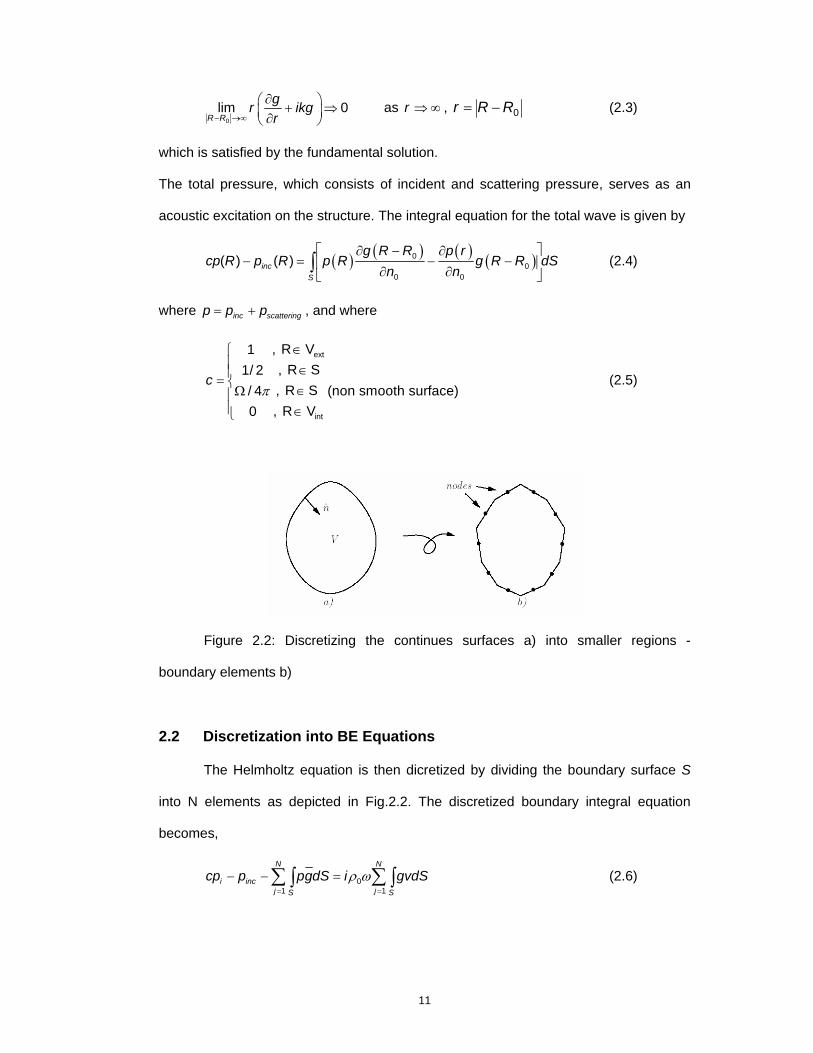
Figure 2.2: Discretizing the continues surfaces a) into smaller regions -
boundary elements b)
2.2 Discretization into BE Equations
The Helmholtz equation is then dicretized by dividing the boundary surface S
into N elements as depicted in Fig.2.2. The discretized boundary integral equation
becomes,
01 1
N N
i incj jS S
cp p pgdS i gvdSρ ω= =
− − =∑ ∑∫ ∫ (2.6)

12
where i indicates field point, j source point and Sj surface element j, and for
convenience, g is defined as
g gn∂
≡∂
(2.7)
Let
j
ij
S
H gdS= ∫ (2.8), j
ijS
G gdS= ∫ (2.9)
Substituting g in Eq. (2.2) to be the monopole Green’s free-space fundamental solution,
it follows that:
( )( )
( )4
j iik R R
ij j iS S S j i
eG gdS g R R dS dSR Rπ
− −
= = − =−∫ ∫ ∫ (2.10)
or, in Cartesian coordinate system,
( ) ( ) ( )
( ) ( ) ( )
2 2 2
2 2 24
j i j i j i
j
ik x x y y z z
ijS
j i j i j i
eG dSx x y y z zπ
− − + − + −
=− + − + −
∫ (2.11)
where Rj is the coordinate vector of the midpoint of element j and Ri is the coordinate
vector of the node i. In the development that follows, four-node iso-parametric
quadrilateral elements are used throughout. To calculate ijH , the derivative g has to be
evaluated
( ) ˆˆ
j j j
Tij
S S S
gH gdS dS g ndSn∂
= = = ∇∂∫ ∫ ∫ (2.12)
where
ˆx
y
z
nn n
n
⎡ ⎤⎢ ⎥= ⎢ ⎥⎢ ⎥⎣ ⎦
(2.13)
and

13
( ) ( ) ( )
( ) ( ) ( ) ( ) ( ) ( )( ) ( ) ( )
( ) ( ) ( ) ( ) ( ) ( )( ) ( ) ( )
( )
2 2 2
2 2 2
2 2 2
2 2 2 2 2 2
2 2 2 2 2 2
1
4
1
4
4
i j i j i j
i j i j i j
i j i j i j
ik x x y y z z
i j i j i j i j i j i j
ik x x y y z z
i j i j i j i j i j i j
ik x x y y z z
i j
xe ikx x y y z z x x y y z z
yeg ikx x y y z z x x y y z z
ze
x x
π
π
π
− − + − + −
− − + − + −
− − + − + −
⎛ ⎞⎜ ⎟− +⎜ ⎟⎜ ⎟− + − + − − + − + −⎝ ⎠⎛ ⎞⎜ ⎟∇ = − +⎜ ⎟⎜ ⎟− + − + − − + − + −⎝ ⎠
−− ( ) ( ) ( ) ( ) ( )2 2 2 2 2 2
1
i j i j i j i j i j
iky y z z x x y y z z
⎡ ⎤⎢ ⎥⎢ ⎥⎢ ⎥⎢ ⎥⎢ ⎥⎢ ⎥⎢ ⎥⎢ ⎥⎢ ⎥
⎛ ⎞⎢ ⎥⎜ ⎟⎢ ⎥+⎜ ⎟⎢ ⎥⎜ ⎟+ − + − − + − + −⎢ ⎥⎝ ⎠⎣ ⎦
(2.14)
For a four-node iso-parametric quadrilateral element, the pressure p and the normal
velocity v at any position on the element can be defined by their nodal values and
linear shape functions, i.e.
( ) [ ]1
21 1 2 2 3 3 4 4 1 2 3 4
3
4
,
vv
v N v N v N v N v N N N Nvv
ξ η
⎡ ⎤⎢ ⎥⎢ ⎥= + + + =⎢ ⎥⎢ ⎥⎢ ⎥⎣ ⎦
(2.15)
( ) [ ]1
21 1 2 2 3 3 4 4 1 2 3 4
3
4
,
pp
p N p N p N p N p N N N Npp
ξ η
⎡ ⎤⎢ ⎥⎢ ⎥= + + + =⎢ ⎥⎢ ⎥⎢ ⎥⎣ ⎦
(2.16)
where the shape functions in the element coordinate system as depicted in Fig. 2.3
are,
( ) ( ) ( ) ( )
( ) ( ) ( ) ( )
1 2
3 4
1 11 1 1 14 41 11 1 1 14 4
N N
N N
ξ η ξ η
ξ η ξ η
= − − = − + −
= + + = − − + (2.17)
The four node quadrilateral element can have any arbitrary orientation in the three-
dimensional space. Using the shape functions (2.17), the integral on the left hand side
of Eq. (2.6), considered over one element j, can be written as:
[ ]1 1
1 2 3 42 21 2 3 4
3 3
4 4
j j
ij ij ijii ijS S
j j
p pp p
pg ds N N N N g dS h h h hp pp p
⎡ ⎤ ⎡ ⎤⎢ ⎥ ⎢ ⎥⎢ ⎥ ⎢ ⎥⎡ ⎤= = ⎣ ⎦⎢ ⎥ ⎢ ⎥⎢ ⎥ ⎢ ⎥⎢ ⎥ ⎢ ⎥⎣ ⎦ ⎣ ⎦
∫ ∫ (2.18)

14
Figure 2.3: Shape function N3 for a four node elements
while that on the right hand side
[ ]1 1
1 2 32 21 2 3 4
3 3
4 4
j j
n
i ij ij ij ijS S
j i
v vv v
gvdS N N N N g dS g g g gv vv v
⎡ ⎤ ⎡ ⎤⎢ ⎥ ⎢ ⎥
⎡ ⎤⎢ ⎥ ⎢ ⎥= = ⎢ ⎥⎢ ⎥ ⎢ ⎥⎣ ⎦⎢ ⎥ ⎢ ⎥⎢ ⎥ ⎢ ⎥⎣ ⎦ ⎣ ⎦
∫ ∫ (2.19)
where
j
kij jk
S
h N g dS= ∫ k = 1,2,3,4 (2.20)
j
kij k j
S
g N g dS= ∫ k = 1,2,3,4 (2.21)
The integration in Eq. (2.18) and (2.19) can be carried out using Gauss points [7,17].
These Gauss points in the iso-parametric system are defined as:
( ) ( ) ( ) ( )
( ) ( ) ( ) ( )
1 1 2 2
3 3 4 4
1 1, 1, 1 , 1,13 31 1, 1,1 , 1, 13 3
ξ η ξ η
ξ η ξ η
= − =
= − = − − (2.22)
Substituting equations (2.18) and (2.19) into equation (2.6) for all elements j, there is
obtained
1 1
1 2 3 4 2 21 2 3 40
1, 13 3
4 4
n
N Nn
ij ij ij ij ij ij ij iji i incj j i j n
nj j
p vp v
c p p h h h h i g g g gp vp v
ρω= ≠ =
⎡ ⎤ ⎡ ⎤⎢ ⎥ ⎢ ⎥
⎡ ⎤ ⎢ ⎥ ⎢ ⎥⎡ ⎤− − = ⎣ ⎦⎢ ⎥ ⎢ ⎥ ⎢ ⎥⎣ ⎦⎢ ⎥ ⎢ ⎥⎢ ⎥ ⎢ ⎥⎣ ⎦ ⎣ ⎦
∑ ∑
(2.23)
Equation (2.23) can be rewritten as
15
1 1
2 21 2 3 4 1 2 3 40
1 13 3
4 4
n
N Nn
ij ij ij ij ij ij ij ij incj j n
nj j
p vp v
h h h h i g g g g pp vp v
ρω= =
⎡ ⎤ ⎡ ⎤⎢ ⎥ ⎢ ⎥⎢ ⎥ ⎢ ⎥⎡ ⎤ ⎡ ⎤= +⎣ ⎦ ⎣ ⎦⎢ ⎥ ⎢ ⎥⎢ ⎥ ⎢ ⎥⎢ ⎥ ⎢ ⎥⎣ ⎦ ⎣ ⎦
∑ ∑ (2.24)
The discretized equation forms a set of simultaneous linear equations, which relates
the pressure pi at field point i due to the boundary conditions p to v at source surface Si
of element i and the incident pressure pinc. In matrix form:
[ ] [ ] 0 incp i v pρ ω= +H G (2.25)
where, H and G are two N x N matrices of influence coefficients, while p and v are
vectors of dimension N representing total pressure and normal velocity on the
boundary elements. This matrix equation can be solved if the boundary condition
v p n= ∂ ∂ and the incident acoustic pressure field pinc are known.
2.3 Implemented BEM Formulation
Based on the BEM formulation for four node iso-parametric quadrilateral linear
acoustic elements, a computational routine written in MATLAB® have been developed
and implemented in order to solve BEM problems for time-harmonic acoustic fluid
domains. The programs routine can be described in the following steps:
• The element discretization is supplied by using commercial meshing software such
as PATRAN®.
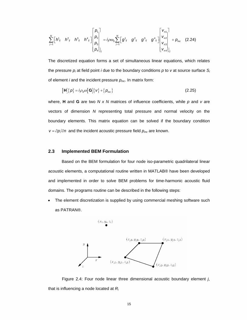
Figure 2.4: Four node linear three dimensional acoustic boundary element j,
that is influencing a node located at Ri

16
• Compute the influence vectors He and Ge for each four node linear three
dimensional acoustic boundary element j, that is influencing a node located at Ri =
(xi, yi, zi) as shown in Fig. 2.4.
• Compute the space angle constant for a node on a non-smooth surface. For a node
coinciding with three or four element corners, the space angle constant Ce is the
quotient of Ω/4π and it’s towards the acoustic medium as shown in Fig. 2.5. The
space angle for a sphere is 4π and for smooth surface the space angle is 2π, and
Ce = 1.
• Assembly all local element influence matrix He and Ge into the global influence
matrix H and G according to each degree of freedom.
• Solve the acoustic BEM equations by adding the known prescribed physical
boundary condition (pressure, normal velocity or impedance), the output are
vectors providing the node boundary pressure and/or the node normal velocity.
• Compute induced acoustic pressure at an arbitrary point in a three dimensional
fluid domain.
Figure 2.5: Space angle constant Ce for a node on a non-smooth surface
2.4 Acoustic BEM Numerical Simulation
In order to verify the correctness of the developed boundary elements acoustic
formulation, a numerical test case is conducted to test the validity of the method. To
avoid complexity, the assumed acoustic source, is monopole source which creates the
acoustic pressure. For a pulsating sphere an exact solution for acoustic pressure p at a

17
distance r from the center of a sphere with radius a pulsating with uniform radial
velocity Ua is
( )0( )1
ik r aa
iz kaap r U er ika
− −=+
(2.26)
where z0 is the acoustic characteristic impedance of the medium and k is the wave
number.
0
0.51
0 0.2 0.4 0.6 0.8 1
0
0.2
0.4
0.6
0.8
1
Discretization of one octant pulsating sphere
Figure 2.6: Discretization of one octant pulsating sphere
Fig. 2.6 shows the discretization of the surface elements of an acoustics
pulsating sphere representing a monopole source. BEM calculation for scattering
pressure from acoustic monopole source will be compared with exact results. The
results are exhibited in Fig.2.7 where the calculated surface pressures on the pulsating
sphere are shown. The calculation was based on the assumption of f=10 Hz, ρ=1.225
Kg/m3, and c=340 m/s which shows the excellent agreement between the
computational procedure developed and the exact one. In Fig. 2.8, the excellent
agreement of BEM calculation for acoustic pressures anywhere in three dimensional
fluid domains with exact calculation serves to validate the developed MATLAB®
program for further utilization.

18
Pressure distribution of pulsating sphere BEM [real part]
13.435
13.44
13.445
13.45
13.455
13.46
13.465
13.47
13.475
13.48
13.485
Pressure distribution of pulsating sphere BEM [magnitude]
74.3
74.35
74.4
74.45
74.5
74.55
Figure 2.7: BEM surface pressure [Real, Imaginary, and Magnitude]

19
Figure 2.8: Comparison of surface pressure on pulsating sphere; exact and
BEM results
2.5 Summary
The excellent agreement of BEM calculation for acoustic pressures in three
dimensional fluid domains with exact calculation has been carried out and a
computational scheme for acoustic boundary element problem has given satisfactory
results. Hence, the objective to develop and validate the boundary element method as
an accurate numerical technique for acoustic domains has been accomplished and
serves to validate the in-house developed BEM computational program written in
MATLAB® for further utilization.

20
CHAPTER THREE FINITE ELEMENT FORMULATION
3.0 Introduction
In this chapter, linear finite element formulation of the structure is described.
The objective is to acquire a finite element program to accurately model the structural
system and obtain pertinent linear theory information needed to couple with the
boundary element method. Some case studies to perform the correctness of the in-
house developed FEM computational program written in MATLAB® are also given.
The finite element method has become a very powerful tool in analyzing static
and dynamic response of structures. The finite element method is capable of handling
complex structural analysis. Many rectangular and triangular type finite elements are
currently being used in commercial and in-house codes. Any type of finite element can
be applied to the following formulation. Two elements selected for this study are
considered here; these are an eight node hexahedral for solid element modeling and
four node quadrilateral for shell element modeling. The FEM formulation on this
chapter is mostly based on Weaver and Johnston [17]. For convenience in further
reference and development, as well as for completeness, these formulations are
summarized in the following sections.
3.1 Eight node hexahedral solid elements
Formulations for iso-parametric hexahedral linear solid elements with three
translational degrees of freedom (DOF) per node are considered.
Figure 3.1: Eight node hexahedral solid elements

21
Nodal quantities will be identified by the node subscript. Thus xi,yi,zi denote the node
coordinates of the ith node, while uxi,uyi,uzi are the nodal displacement DOFs. The
shape function for the ith node is denoted by Ni. The element geometry is described by:
1
1 2 2
1 2
1 2
1 1 ... 11.........
n
n
n n
Nx x x Nxy y yyz z z Nz
⎡ ⎤ ⎡ ⎤⎡ ⎤⎢ ⎥ ⎢ ⎥⎢ ⎥⎢ ⎥ ⎢ ⎥⎢ ⎥ =⎢ ⎥ ⎢ ⎥⎢ ⎥⎢ ⎥ ⎢ ⎥⎢ ⎥
⎢ ⎥ ⎢ ⎥ ⎢ ⎥⎣ ⎦ ⎣ ⎦ ⎣ ⎦
M (3.1)
The four rows of this matrix relation express the geometric conditions which the shape
functions must identically satisfy.
1
1n
ii
N=
= ∑ 1
n
i ii
x x N=
= ∑ 1
n
i ii
y y N=
= ∑ 1
n
i ii
z z N=
= ∑ (3.2)
The first one: sum of shape functions must be unity, is an essential part of the
verification of completeness. The displacement interpolation is
11 2
21 2
1 2
x x x xn
y y y yn
z z z znn
Nu u u u
Nu u u u
u u u u N
⎡ ⎤⎡ ⎤ ⎡ ⎤ ⎢ ⎥⎢ ⎥ ⎢ ⎥ ⎢ ⎥=⎢ ⎥ ⎢ ⎥ ⎢ ⎥⎢ ⎥ ⎢ ⎥ ⎢ ⎥⎣ ⎦ ⎣ ⎦ ⎢ ⎥⎣ ⎦
K
KM
K
(3.3)
The three rows of this matrix relation express the interpolation conditions
1
n
x x iii
u u N=
= ∑ 1
n
y y iii
u u N=
= ∑ 1
n
z z iii
u u N=
= ∑ (3.4)
The identical structure of the geometry definition and displacement interpolation
characterizes an iso-parametric element. The interpolation functions for eight node
solid element are:
( )( )( ) ( )( )( )
( )( )( ) ( )( )( )
( )( )( ) ( )( )( )
( )( )( ) ( )( )( )
1 5
2 6
3 7
4 8
1 11 1 1 1 1 18 81 11 1 1 1 1 18 81 11 1 1 1 1 18 81 11 1 1 1 1 18 8
e e
e e
e e
e e
N N
N N
N N
N N
ξ η ζ ξ η ζ
ξ η ζ ξ η ζ
ξ η ζ ξ η ζ
ξ η ζ ξ η ζ
= − − − = − − +
= + − − = + − +
= + + − = + + +
= − + − = − + +
(3.5)
We restrict attention to linear elastostatic analysis without initial stresses. For a general
solid element the proportional matrix can be presented as:

22
( )( )
1 0 0 01 0 0 0
1 0 0 0(1 2 )0 0 0 0 0
21 1 2(1 2 )0 0 0 0 0
2(1 2 )0 0 0 0 0
2
v v vv v vv v v
vEDv v
v
v
−⎡ ⎤⎢ ⎥−⎢ ⎥⎢ ⎥−⎢ ⎥
−⎢ ⎥= ⎢ ⎥− − ⎢ ⎥−⎢ ⎥
⎢ ⎥⎢ ⎥−⎢ ⎥⎢ ⎥⎣ ⎦
(3.6)
The strains are related to the element node displacements by
e= ∇B N (3.7)
where
0 0
0 0
0 0
x
y
z
y x
z x
z y
∂⎡ ⎤⎢ ⎥∂⎢ ⎥
∂⎢ ⎥⎢ ⎥∂⎢ ⎥
∂⎢ ⎥⎢ ⎥∂⎢ ⎥∇ =∂ ∂⎢ ⎥
⎢ ⎥∂ ∂⎢ ⎥∂ ∂⎢ ⎥
⎢ ⎥∂ ∂⎢ ⎥
∂ ∂⎢ ⎥⎢ ⎥∂ ∂⎢ ⎥⎣ ⎦
, ( ) 1T
x
y
z
ξ
η
ζ
−
⎡ ⎤∂⎡ ⎤∂⎢ ⎥⎢ ⎥ ∂∂ ⎢ ⎥⎢ ⎥⎢ ⎥∂ ∂⎢ ⎥ = ⎢ ⎥⎢ ⎥∂ ∂⎢ ⎥⎢ ⎥⎢ ⎥∂ ∂⎢ ⎥⎢ ⎥⎢ ⎥∂ ∂⎣ ⎦ ⎢ ⎥⎣ ⎦
J ,
x x x
y y y
z z z
ξ η ζ
ξ η ζ
ξ η ζ
⎡ ⎤∂ ∂ ∂⎢ ⎥∂ ∂ ∂⎢ ⎥⎢ ⎥∂ ∂ ∂
= ⎢ ⎥∂ ∂ ∂⎢ ⎥⎢ ⎥∂ ∂ ∂⎢ ⎥∂ ∂ ∂⎢ ⎥⎣ ⎦
J (3.8)
and for deriving the consistent mass matrix the interpolation function is rearranged as
11 8
21 8
1 824
0 0 0 00 0 0 00 0 0 0
x
y
z
uu N N
uu N N
N Nu u
⎡ ⎤⎡ ⎤ ⎡ ⎤ ⎢ ⎥⎢ ⎥ ⎢ ⎥ ⎢ ⎥=⎢ ⎥ ⎢ ⎥ ⎢ ⎥⎢ ⎥ ⎢ ⎥ ⎢ ⎥⎣ ⎦⎣ ⎦ ⎢ ⎥⎣ ⎦
K
KM
K
(3.9)
The element stiffness and mass matrix is formally given by the volume integral where
the integral is taken over the element volume.
e
e T
V
dV= ∫K B DB (3.10)
and
e
e T
V
dVρ= ∫M N N (3.11)
By applying gauss integration the element stiffness and mass matrix became:

23
( ) ( ) ( )
1 1 1
1 1 1
, , , , , ,T d d dξ η ζ ξ η ζ ξ η ζ ξ η ζ− − −
= ∫ ∫ ∫K B DB J
, , , , , ,
1 1 1
n n nT
j k l j k l j k l j k ll k j
R R R= = =
= ∑∑∑K B DB J (3.12)
and
( ) ( ) ( )
1 1 1
1 1 1
, , , , , ,T d d dρ ξ η ζ ξ η ζ ξ η ζ ξ η ζ− − −
= ∫ ∫ ∫M N N J
, , , , , ,
1 1 1
n n nT
j k l j k l j k l j k ll k j
R R Rρ= = =
=∑∑∑M N N J (3.13)
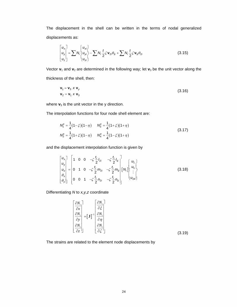
3.2 Four node quadrilateral shell elements
Formulations for Iso-parametric four node quadrilateral linear shell elements
with three translational and two rotational degrees of freedom (DOF) per node are
considered.
Figure 3.2: Four node quadrilateral shell elements
For a general shell element the proportional matrix can be presented as:
2
1 0 0 01 0 0 0
10 0 0 02
(1 ) 10 0 0 02
10 0 0 02
vv
vE kDv v
kv
k
⎡ ⎤⎢ ⎥⎢ ⎥⎢ ⎥−⎢ ⎥
= ⎢ ⎥− −⎢ ⎥
⎢ ⎥⎢ ⎥
−⎢ ⎥⎢ ⎥⎣ ⎦
(3.14)
x
y
z
24
The displacement in the shell can be written in the terms of nodal generalized
displacements as:
2 1 1 22 2
x xi
y i yi i i i i i i
z zi
u ut tu N u N N
u u
ζ θ ζ θ⎡ ⎤ ⎧ ⎫⎢ ⎥ ⎪ ⎪
= − +⎨ ⎬⎢ ⎥⎪ ⎪⎢ ⎥
⎣ ⎦ ⎩ ⎭
∑ ∑ ∑v v (3.15)
Vector v1 and v2 are determined in the following way; let v3 be the unit vector along the
thickness of the shell, then:
1 3
2 1 3
yx
x
=
=
v v vv v v
(3.16)
where v3 is the unit vector in the y direction.
The interpolation functions for four node shell element are:
( )( ) ( )( )
( )( ) ( )( )
1 3
2 4
1 11 1 1 14 41 11 1 1 14 4
e e
e e
N N
N N
ξ η ξ η
ξ η ξ η
= − − = + +
= + − = − + (3.17)
and the displacement interpolation function is given by
[ ]
2 11
12 1
242 1
1 0 02 2
0 1 02 2
0 0 12 2
i ix i iy
i ii i iz
xi i
i iy
t tu l l uuut tm m Nu
t t un n
ζ ζ
ζ ζθ
ζ ζθ
⎡ ⎤⎡ ⎤ − −⎢ ⎥ ⎧ ⎫⎢ ⎥⎢ ⎥ ⎪ ⎪⎢ ⎥ ⎪ ⎪⎢ ⎥⎢ ⎥ = − − ⎨ ⎬⎢ ⎥⎢ ⎥ ⎪ ⎪⎢ ⎥⎢ ⎥ ⎪ ⎪⎢ ⎥ ⎩ ⎭⎢ ⎥ − −⎢ ⎥ ⎢ ⎥⎣ ⎦ ⎣ ⎦
M (3.18)
Differentiating N to x,y,z coordinate
[ ] 1
ii
i i
ii
NNxN Ny
NNz
ξ
η
ζ
−
⎡ ⎤∂⎡ ⎤∂⎢ ⎥⎢ ⎥ ∂∂ ⎢ ⎥⎢ ⎥⎢ ⎥∂ ∂⎢ ⎥ = ⎢ ⎥⎢ ⎥∂ ∂⎢ ⎥⎢ ⎥⎢ ⎥∂∂⎢ ⎥⎢ ⎥⎢ ⎥ ∂∂⎣ ⎦ ⎣ ⎦
J
(3.19)
The strains are related to the element node displacements by