Embed Size (px)
Citation preview

Correlation Clustering: from Theory to Practice
Francesco Bonchi Yahoo Labs, Barcelona
David Garcia-Soriano Yahoo Labs, Barcelona
Edo Liberty Yahoo Labs, NYC

Plan of the talk
2
Part 1: Introduction and fundamental results › Clustering: from the Euclidean setting to the graph setting
› Correlation clustering: motivations and basic definitions,
› Fundamental results
› The Pivot Algorithm
Part 2: Correlation clustering variants
› Overlapping, On-line, Bipartite, Chromatic
› Clustering aggregation
Part 3: Scalability for real-world instances
› Real-world application examples
› Scalable implementation
› Local correlation clustering

Part I : Introduction and fundamental results
3
Edo Liberty Yahoo Labs, NYC

Clustering, in general
5
Partition a set of objects such that “similar” objects are grouped together and “dissimilar” objects are set apart.
Setting
Objective function
Algorithm

Euclidean Setting
6
Points
Small indicates the two points are “similar”

Euclidean Setting
7
Clusters Points
A cluster is a set of points

Euclidean Setting
8
Centers
Points Clusters
Each cluster has a cluster center

Euclidean objectives
9
K-means objective
Points
Centers
Clusters

Euclidean objectives
10
K-median objective
Points
Centers
Clusters

Euclidean objectives
11
K-centers objective
Points
Centers
Clusters

Graph setting
12
Nodes Edges
means the two nodes are “similar”
Graph setting
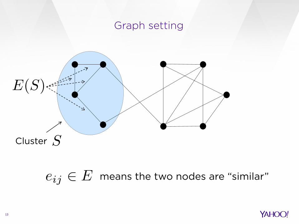
13
Cluster
means the two nodes are “similar”

Graph setting
14
We want and large and small
Cluster
Graph objectives
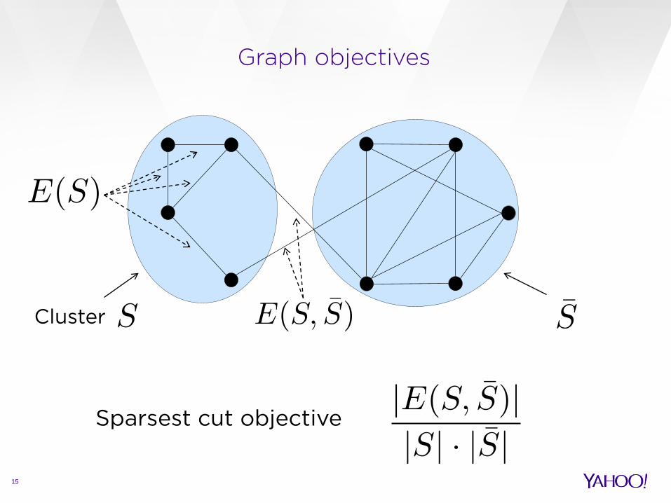
15
Cluster
Sparsest cut objective
Graph objectives
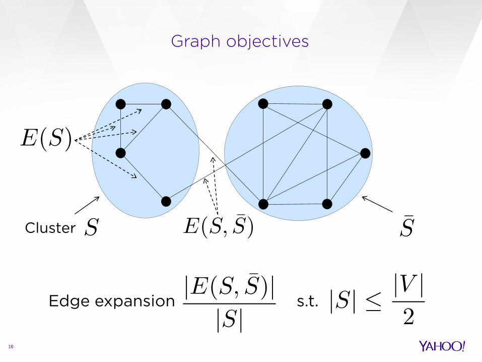
16
Cluster
Edge expansion s.t.

Graph objectives
17
Cluster
Graph Conductance s.t.

Graph objectives
18
k-balanced partitioning Where
Graph objectives
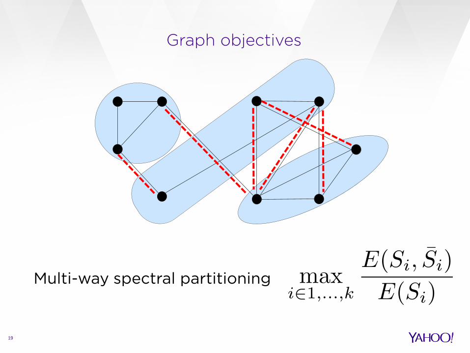
19
Multi-way spectral partitioning
Correlation Clustering objective
20
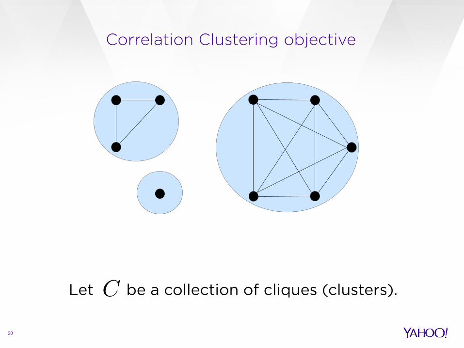
Let be a collection of cliques (clusters).
Correlation Clustering objective
21
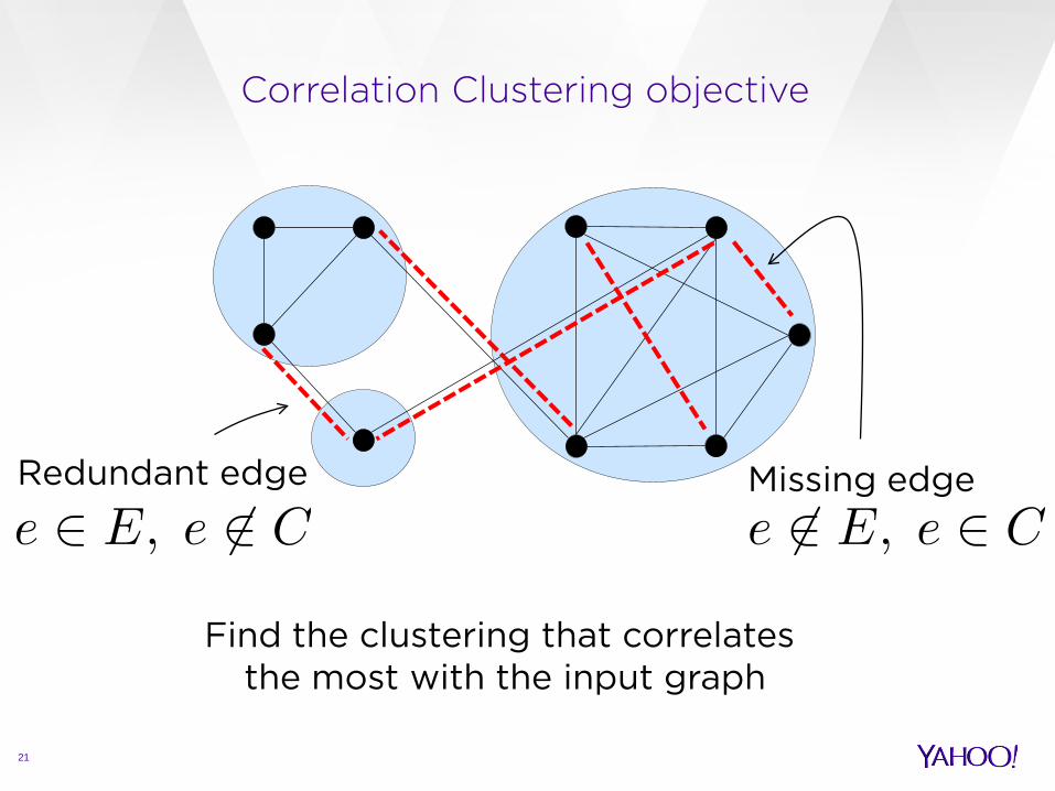
Find the clustering that correlates the most with the input graph
Redundant edge Missing edge
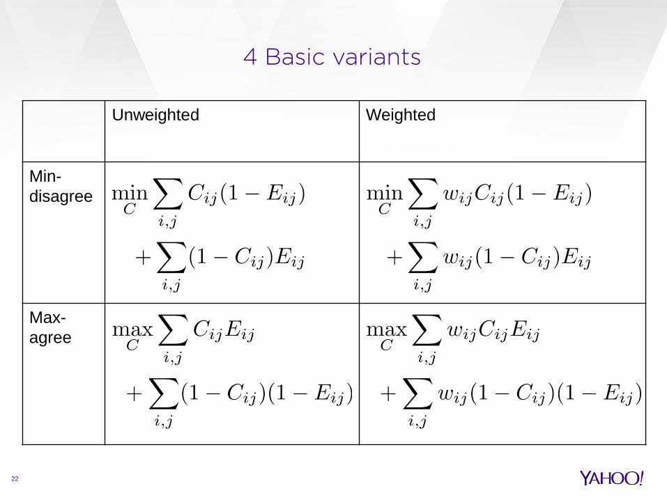
4 Basic variants
22
Unweighted Weighted
Min-disagree
Max-agree
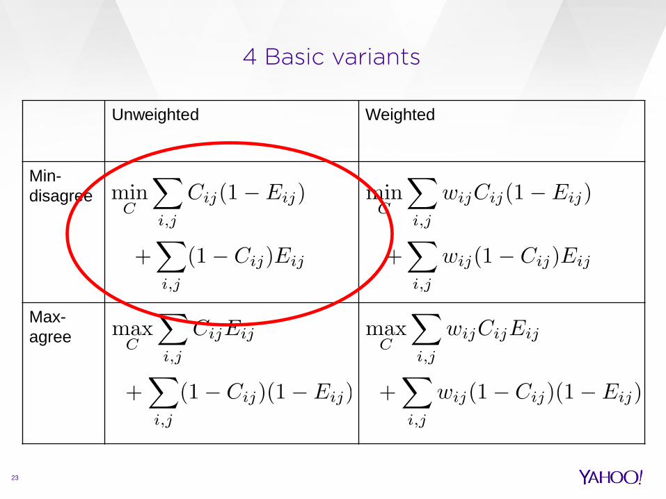
4 Basic variants
23
Unweighted Weighted
Min-disagree
Max-agree
Correlation Clustering objective
24
Important points to notice There is no limitation on the number of clusters and no limitation on their sizes
For example: the best solution could be 1 giant cluster n singletons

Document de-duplication
25

Document de-duplication
26
They are not identical
Document de-duplication
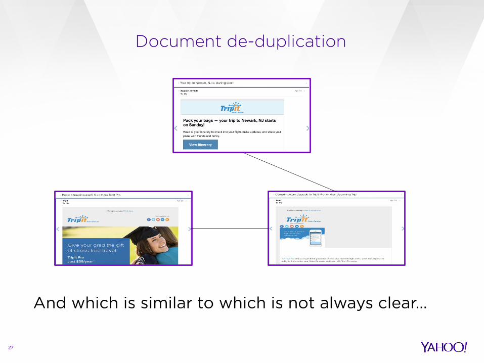
27
And which is similar to which is not always clear…

Document de-duplication
28

Motivation from machine learning
29

Motivation from machine learning
30
Input graph (Result of classifier)
Space of valid clustering solutions
True clustering (unknown)
Output of the clustering algorithm
Classification Errors
Clustering Errors w.r.t. input
Clustering Errors w.r.t. true clustering

Some bad news : min-disagree
31
Unweighted complete graphs - NP-hard (BBC02) › Reduction from “Partition into Triangles” Unweighted general graphs - APX-hard (DEFI06)
› Reduction from multiway cuts. Weighted general graphs - APX-hard (DEFI06)
› Reduction from multiway cuts.

An algorithms is a approximation if:
Algorithms for unweighted min-disagree
32
Paper Approximation Running time [BBC02] [DEFI06] LP [CGW03] LP [ACNA05] LP [ACNA05]
[AL09]

Algorithm warm-up
33
From
Correlation clustering, 2002 Nikhil Bansal, Avrim Blum, and Shuchi Chawla.

Algorithm warm-up
34
Algorithm warm-up
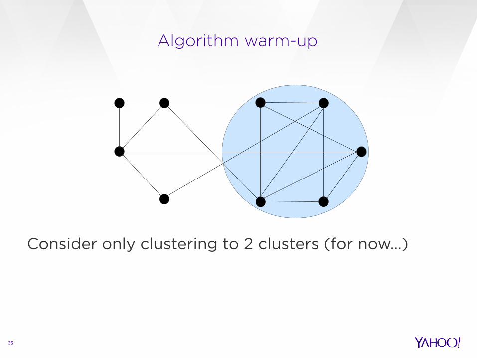
35
Consider only clustering to 2 clusters (for now…)

Algorithm warm-up
36
Consider all clustering to 2 clusters of the form

Algorithm warm-up
37
Consider the one whose neighborhood disagrees the least with the best clustering. (Here )

Algorithm warm-up
38
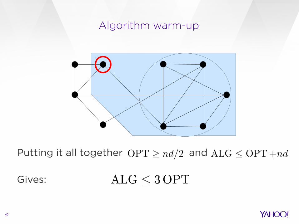
Each node “contributes” at least mistakes. Therefore

Algorithm warm-up
39
On the other hand (Each of the disagreements adds at most errors)
Algorithm warm-up
40
Putting it all together and
Gives:

LP based solutions
41
Erik D. Demaine, Dotan Emanuel, Amos Fiat, Nicole Immorlica
Correlation clustering in general weighted graphs, 2006
Moses Charikar, Venkatesan Guruswami, and Anthony Wirth. Clustering with qualitative information, 2003
Nir Ailon, Moses Charikar, Alantha Newman 2005
Aggregating inconsistent information: ranking and clustering

LP relaxation
42
Minimize
s.t.

LP relaxation
43
Minimize
s.t. instead of triangle inequality The solution is at least as good as But, it’s fractional…
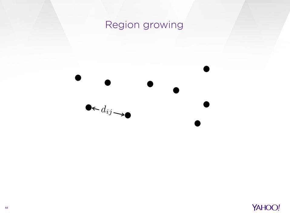
Region growing
44
Region growing
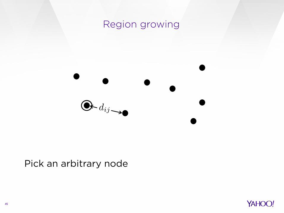
45
Pick an arbitrary node

Region growing
46
Start growing a ball around it

Region growing
47
Stop when some condition holds.
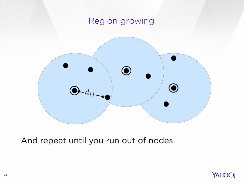
Region growing
48
And repeat until you run out of nodes.

Some good and some bad news
49
Good news: [DEFI06] [CGW03] For weighted graphs we get:
[CGW03] For unweighted graphs we get:

Pivot
50
Nir Ailon, Moses Charikar, Alantha Newman 2005 Aggregating inconsistent information: ranking and clustering
Pivot
51

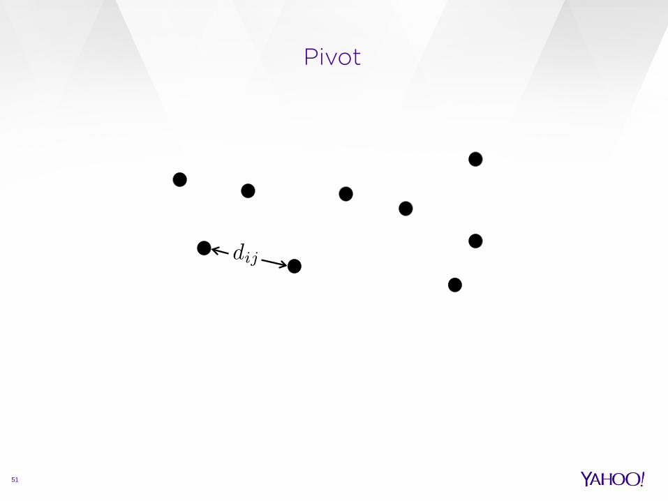
Pivot
52
Pick a node ( ) uniformly at random

Pivot
53
With probability for all
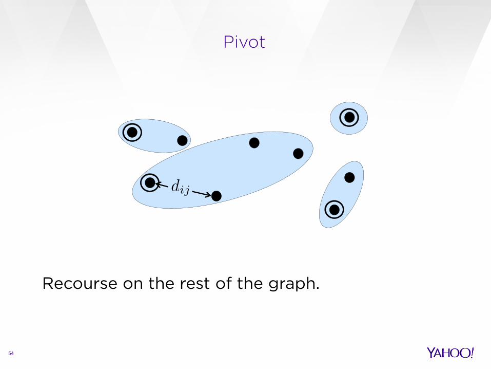
Pivot
54
Recourse on the rest of the graph.
Some good and some bad news
55
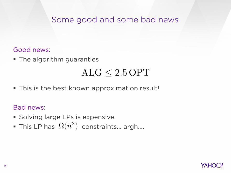
Good news: The algorithm guaranties
This is the best known approximation result! Bad news: Solving large LPs is expensive. This LP has constraints… argh….

Pivot – skipping the LP
56
Nir Ailon, Moses Charikar, Alantha Newman 2005 Aggregating inconsistent information: ranking and clustering

Pivot
57
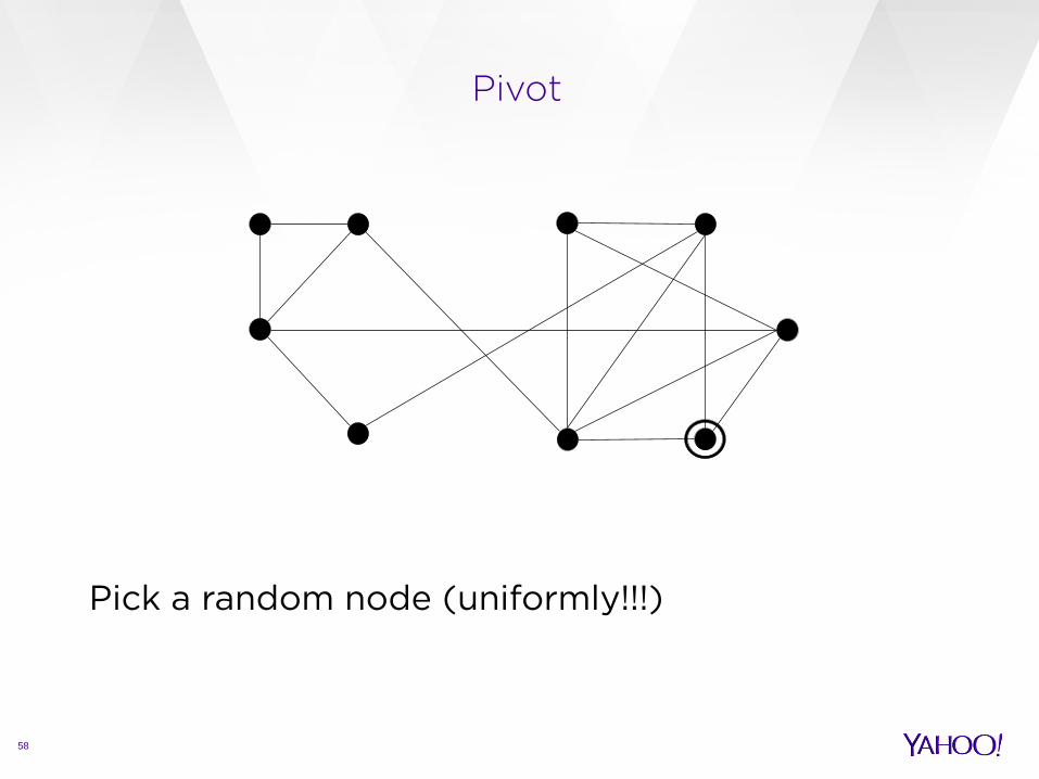
Pivot
58
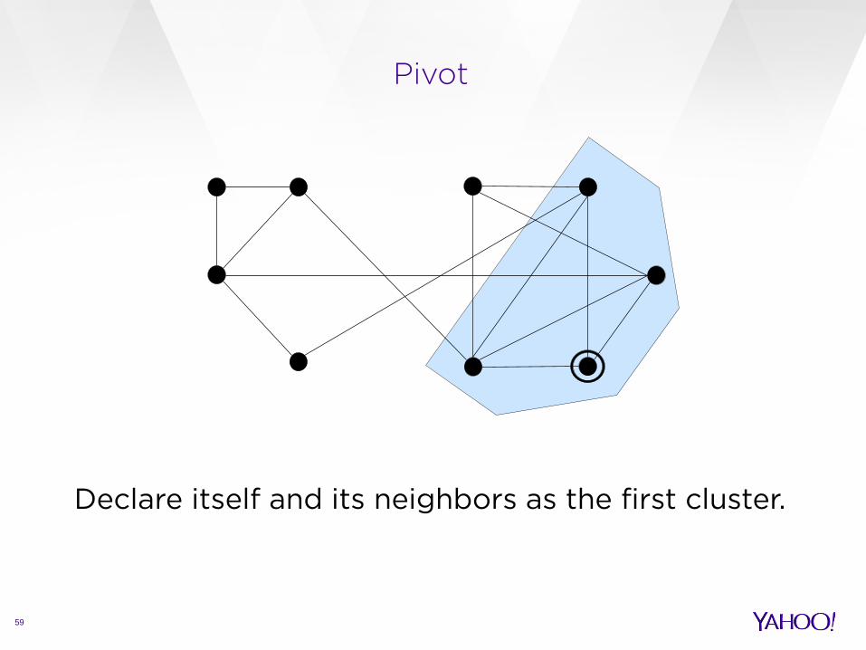
Pick a random node (uniformly!!!)
Pivot
59
Declare itself and its neighbors as the first cluster.
Pivot
60
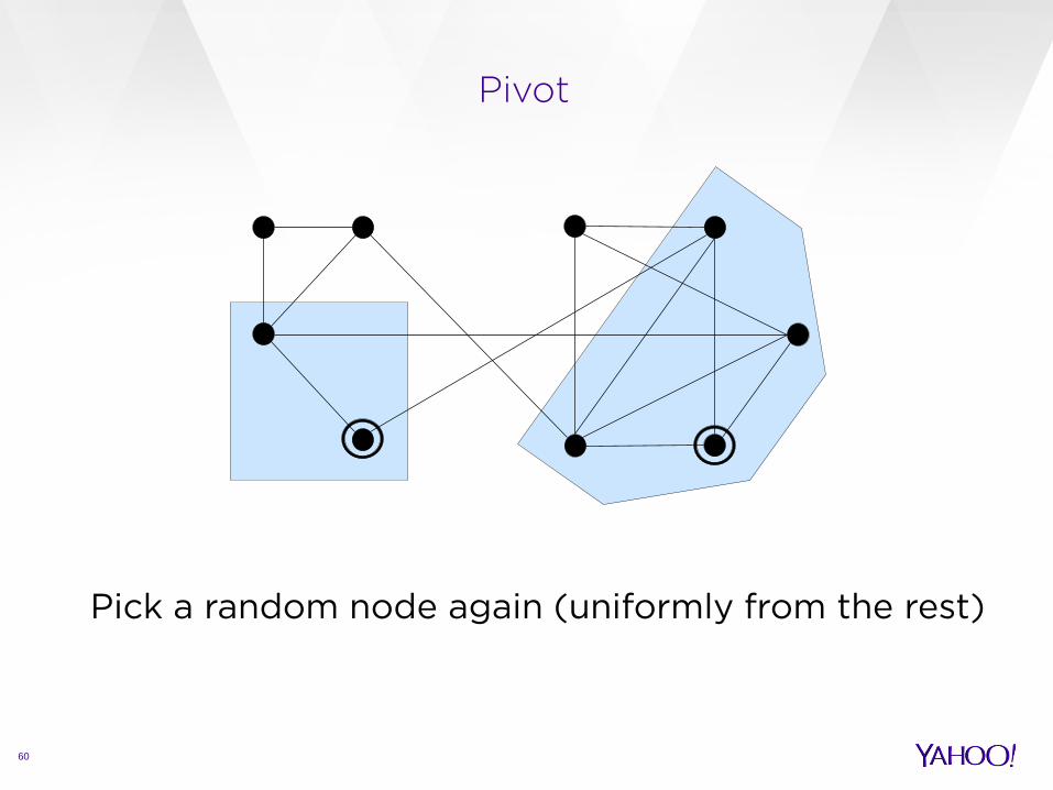
Pick a random node again (uniformly from the rest)
Pivot
61
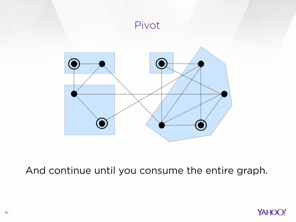
And continue until you consume the entire graph.

Some good and some bad news
62
Good news: The algorithm guaranties
Running time is , very efficient!!
Bad news: Works only for complete unweighted graphs

References
63
Nikhil Bansal, Avrim Blum, and Shuchi Chawla 2002 Correlation clustering Erik Demaine, Dotan Emanuel, Amos Fiat, Nicole Immorlica 2006 Correlation clustering in general weighted graphs Moses Charikar, Venkatesan Guruswami, Anthony Wirth 2003 Clustering with qualitative information.
Nir Ailon, Moses Charikar, Alantha Newman 2005 Aggregating inconsistent information: ranking and clustering
Further reading
64
Ioannis Giotis, Venkatesan Guruswami 2006 Correlation Clustering with a Fixed Number of Clusters Nir Ailon, Edo Liberty 2009 Correlation Clustering Revisited: The "True" Cost of Error Minimization Problems. Anke van Zuylen, David P. Williamson 2009 Deterministic Pivoting Algorithms for Constrained Ranking and Clustering Problems Claire Mathieu, Warren Schudy 2010 Correlation Clustering with Noisy Input Claire Mathieu, Ocan Sankur, Warren Schudy 2010 Online Correlation Clustering Nir Ailon, Noa Avigdor-Elgrabli, Edo Liberty, Anke van Zuylen 2012 Improved Approximation Algorithms for Bipartite Correlation Clustering. Nir Ailon and Zohar Karnin 2012 No need to choose: How to get both a PTAS and Sublinear Query Complexity

Part I I : Correlation clustering variants
65
Francesco Bonchi Yahoo Labs, Barcelona

Correlation clustering variants
66
Overlapping Chromatic On-line Bipartite Clustering aggregation

Overlapping correlation clustering
67
F. Bonchi, A. Gionis, A. Ukkonen: Overlapping Correlation Clustering ICDM 2011

68
overlapping clusters are very natural social networks proteins documents
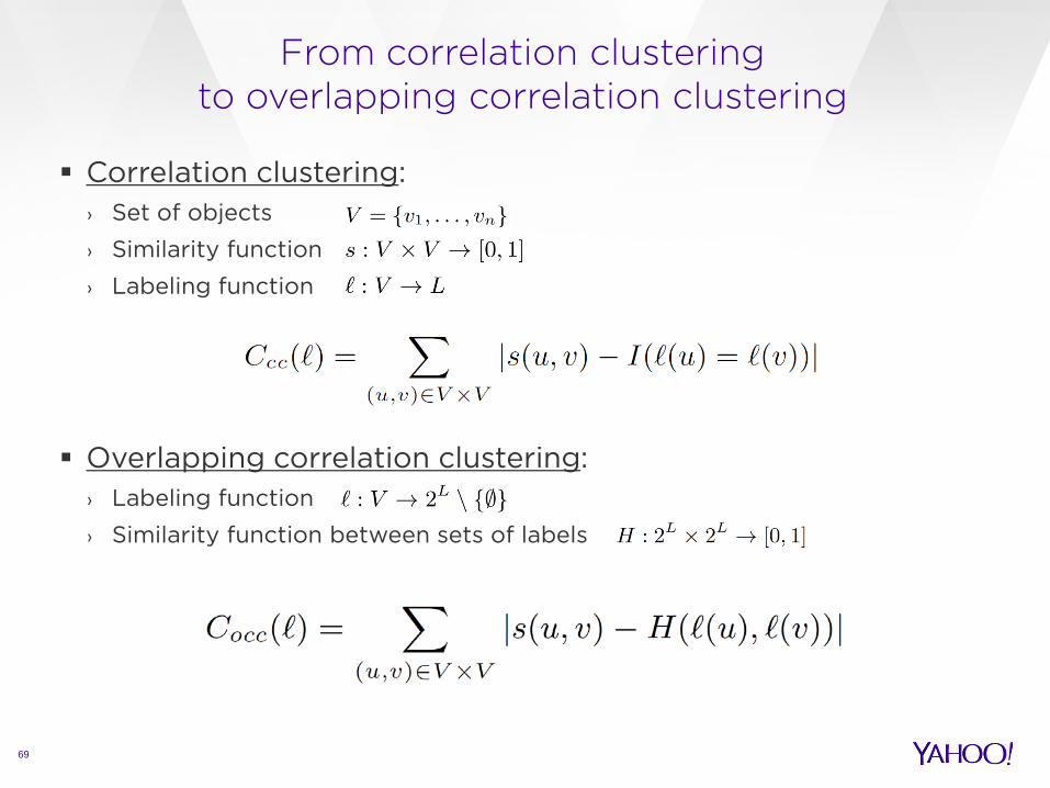
From correlation clustering to overlapping correlation clustering
69
Correlation clustering: › Set of objects
› Similarity function
› Labeling function
Overlapping correlation clustering: › Labeling function
› Similarity function between sets of labels

OCC problem variants
70
Based on these choices: › Similarity function s takes values in
› Similarity function s takes values in
› Similarity function H is the Jaccard coefficient
› Similarity function H is the intersection indicator
› Constraint on the maximum number of labels per object
› Special cases:
normal Correlation Clustering
no constraint
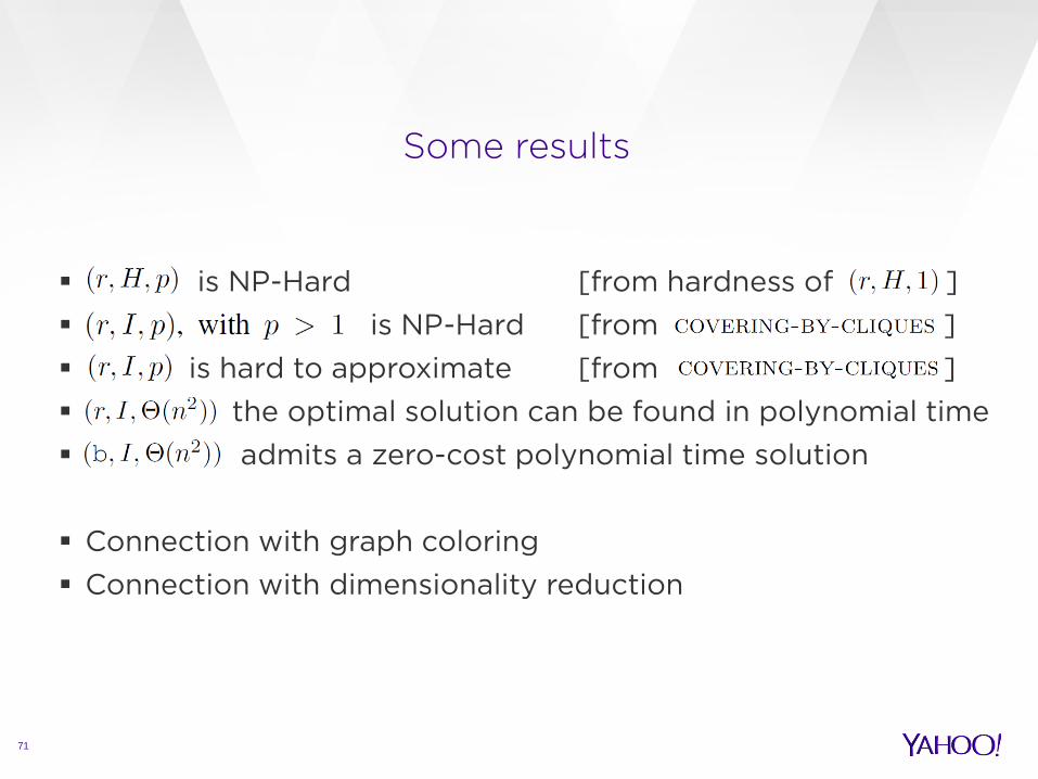
Some results
71
is NP-Hard [from hardness of ] is NP-Hard [from ] is hard to approximate [from ] the optimal solution can be found in polynomial time admits a zero-cost polynomial time solution
Connection with graph coloring Connection with dimensionality reduction

Local-search algorithm
72
We observe that cost can be rewritten as:
where

Local step for Jaccard
73
› Given
› Find that minimizes
is NP-Hard › generalization of “Jaccard median” problem*
› non-negative least squares + post-processing of the fractional solution
F. Chierichetti, R. Kumar, S. Pandey, S. Vassilvitskii: Finding the Jaccard Median. SODA 2010

Local step for set intersection indicator
74
problem Inapproximable within a constant factor approximation by Greedy algorithm
Experiments on ground-truth overlapping clusters
75
Two datasets from multilable classification
› EMOTION: 593 objects, 6 labels
› YEAST: 2417 objects, 14 labels
Input similarity s(u,v) is the Jaccard coefficient of the labels of u and v in the ground truth

Experiments on ground-truth overlapping clusters
76

Application: overlapping clustering of trajectories
77
Starkey project dataset containing the radio-telemetry locations of elks, deer, and cattle.
88 trajectories › 33 elks
› 14 deers
› 41 cattles
80K (x,y,t) observations (909 observations per trajectory in avg) Use EDR* as trajectory distance function, normalized to be in [0,1]
Experiment setting: k = 5, p = 2, Jaccard
* L. Chen, M. T. Özsu, V. Oria: Robust and Fast Similarity Search for Moving Object Trajectories. SIGMOD 2005
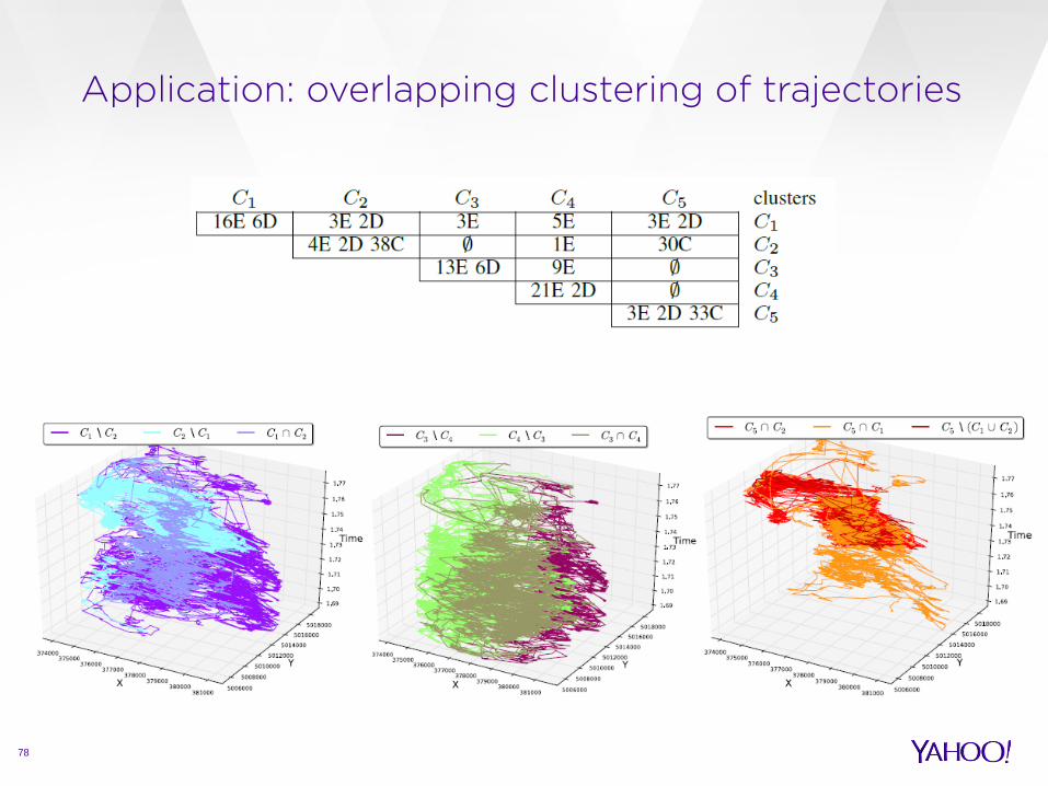
Application: overlapping clustering of trajectories
78

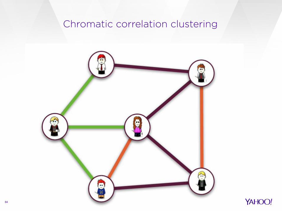
Chromatic correlation clustering
79
F. Bonchi, A. Gionis, F. Gullo, A. Ukkonen: Chromatic correlation clustering
KDD 2012
80
heterogeneous data objects of single type associations between objects are categorical can be viewed as edges with colors in a graph

81
Example: social networks

82
Example : protein interaction networks
83
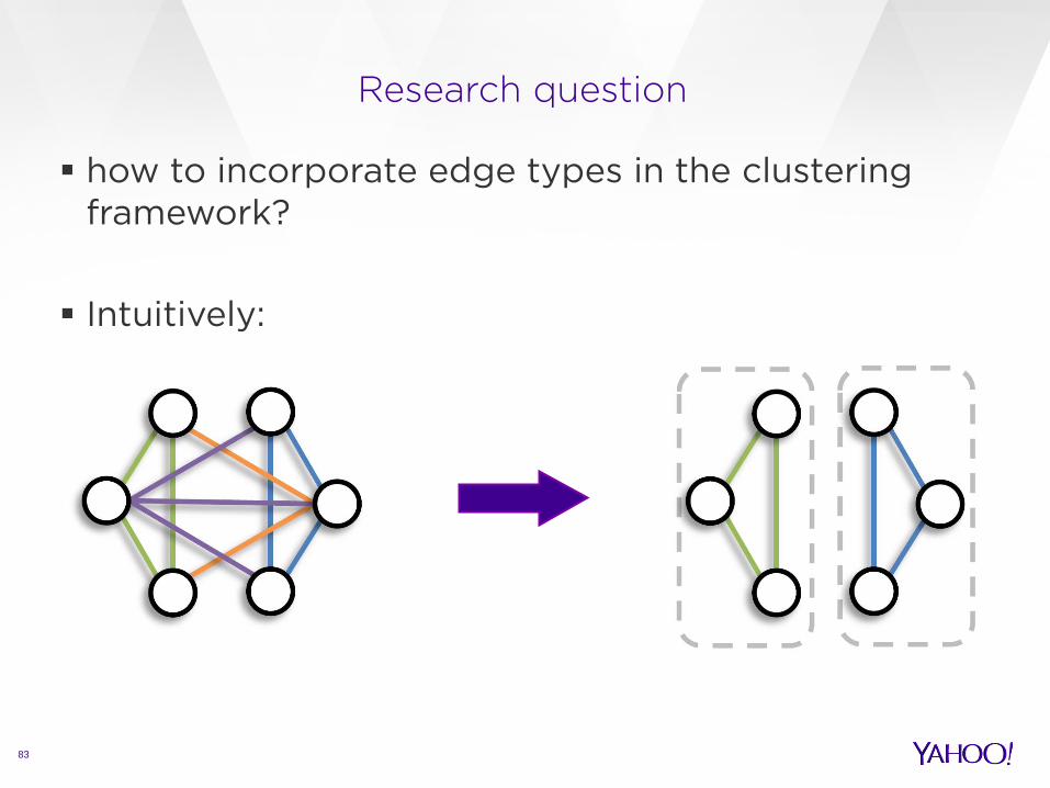
Research question
how to incorporate edge types in the clustering framework? Intuitively:
84
Chromatic correlation clustering

85
Chromatic correlation clustering

86
Cost of chromatic correlation clustering

87
Cost of chromatic correlation clustering
From correlation clustering to chromatic correlation clustering
88
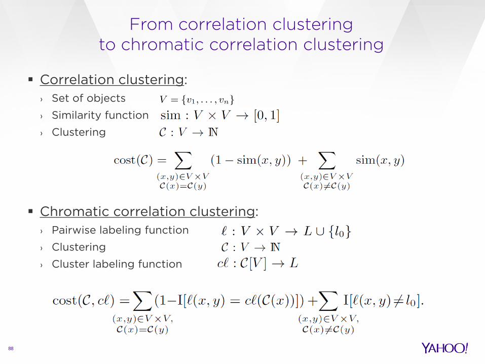
Correlation clustering: › Set of objects
› Similarity function
› Clustering
Chromatic correlation clustering: › Pairwise labeling function
› Clustering
› Cluster labeling function

89
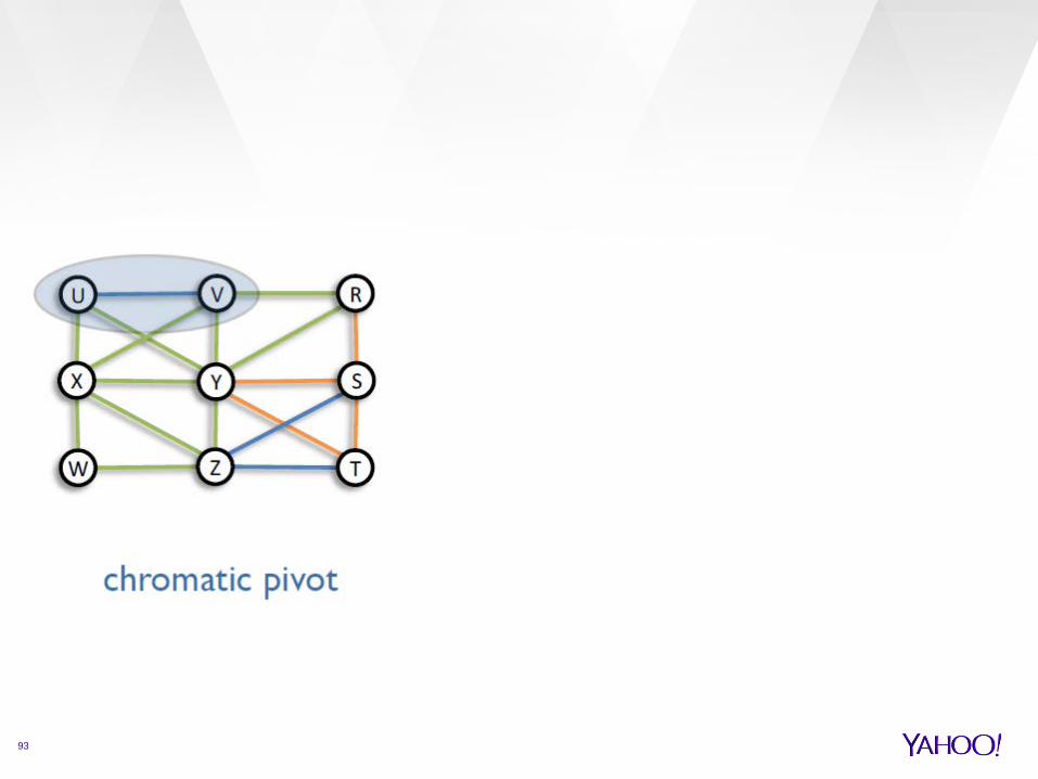
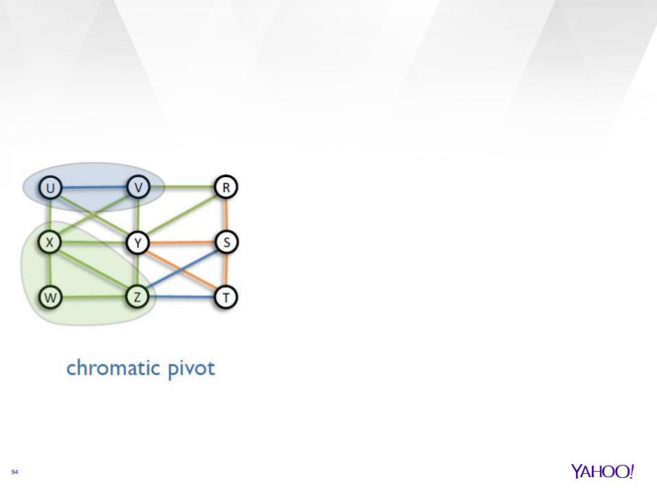
chromatic PIVOT algorithm
Pick a random edge (u,v), of color c Make a cluster with u,v and all neighbors w, such that
(u,v,w) is monochromatic assign color c to the cluster repeat until left with empty graph
approximation guarantee 6(2D-1)
› where D is the maximum degree
Time complexity

90
how good is this bound ?

91
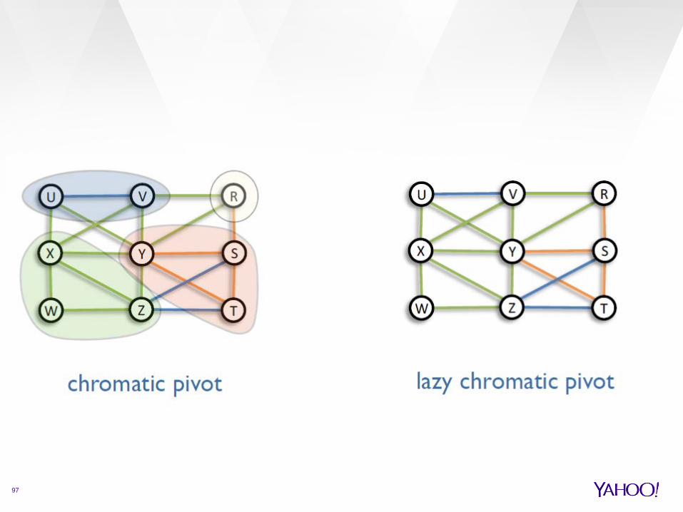
Lazy chromatic pivot
Same scheme as Chromatic Pivot with two differences:
The way how the pivot (x,y) is picked: not uniformly at random, but with probability
proportional to the maximum chromatic degree
The way how the cluster is built around (x,y): not only vertices forming monochromatic triangles
with the pivots, but also vertices forming monochromatic triangles with non-pivot vertices belonging to the cluster.
Time complexity

92
93
94

95

96
97

98

99

100
101
An algorithm for finding a predefined number of clusters
Based on the alternating-minimization paradigm: › Start with a random clustering with K clusters › Keep fixed vertex-to-cluster assignments and optimally update
label-to-cluster assignments › Keep fixed label-to-cluster assignments and optimally update
vertex-to-cluster assignments › Alternately repeat the two steps until convergence
Guaranteed to converge to a local minimum of the
objective function
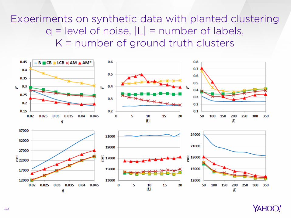
Experiments on synthetic data with planted clustering q = level of noise, |L| = number of labels,
K = number of ground truth clusters
102

Experiments on real data
103
104
Extension: multi-chromatic correlation clustering (to appear)
object relations can be expressed by more than one label i.e., the input to our problem is an edge-labeled graph whose
edges may have multiple labels.
Extending chromatic correlation clustering by: 1. allowing to assign a set of labels to each cluster (instead of
a single label) 2. measuring the intra-cluster label homogeneity by means of
a distance function between sets of labels

From chromatic correlation clustering to multi-chromatic correlation clustering
105
Chromatic correlation clustering: › Set of objects
› Pairwise labeling function
› Clustering
› Cluster labeling function
Multi-chromatic correlation clustering:
› Pairwise labeling function
› Distance between set of labels
› Cluster labeling function

106
As distance between sets of labels we adopt Hamming distance A consequence is that inter-cluster edges cost the
number of labels they have plus one

107
Multi-chromatic pivot
Pick randomly a pivot Add all vertices such that The cluster is assigned the set of colors
approximation guarantee 6|L|(D-1)
› where D is the maximum degree
Online correlation clustering
108
C. Mathieu, O. Sankur, W. Schudy: Online correlation clustering
STACS 2010

Online correlation clustering
Vertices arrive one by one. The size of the input is unknown. Upon arrival of a vertex v, an online algorithm can
› Create a new cluster v.
› Add v to an existing cluster.
› Merge any pre-existing clusters.
› Split a pre-existing cluster

Main results
110
An online algorithm is c-competitive if on any input I , the algorithm outputs a clustering ALG(I) s.t.
profit(ALG(I)) ≥ c · profit(OPT(I)) where OPT(I) is the offline optimum. Main results:
› is hopeless: O(n)-competitive and this is proved optimal.
› For • Greedy 0.5-competitive
• No algorithm can be better than 0.834-competitive
• (0.5+c)-competitive randomized algorithm

111

112

113
If profit(OPT) ≤ (1 − α)|E|, has competitive ratio > 0.5
IDEA: design an algorithm with competitive ratio > 0.5 when profit(OPT) > (1 − α)|E|
is (0.5 + ε)-competitive.

Algorithm Dense
114
Reminder: focus on instances where profit(OPT) > (1 − α)|E| Fix When new vertices arrive put them in a singleton cluster At times Compute (near) Merge clusters as explained next

115
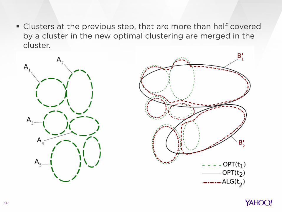
Suppose we start with OPT at time t1. Until time t2, we put all new vertices to singletons.
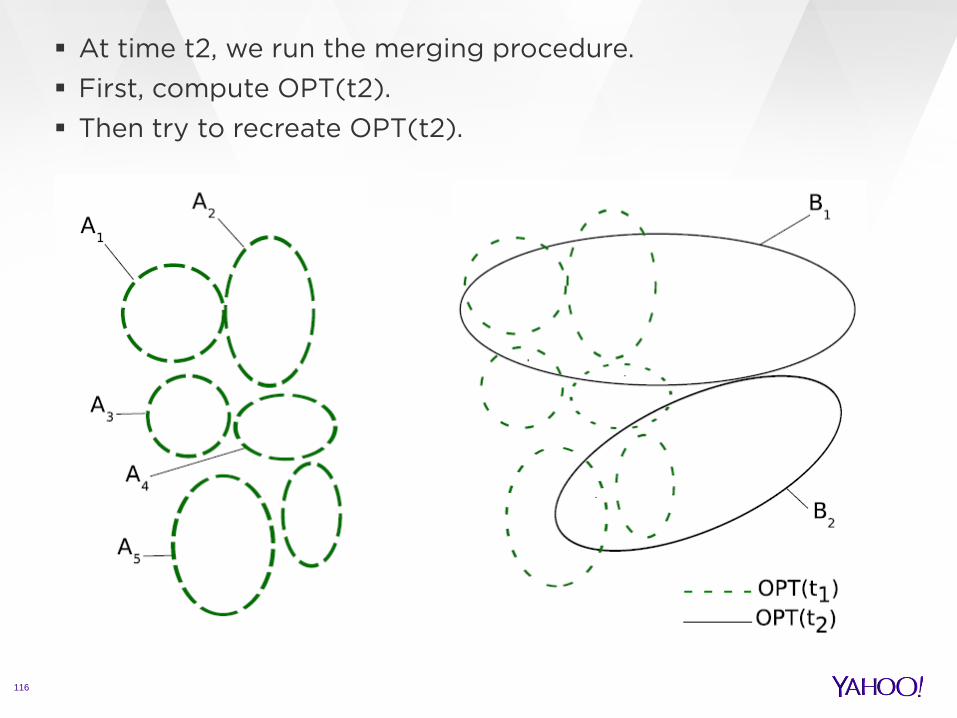
116
At time t2, we run the merging procedure. First, compute OPT(t2). Then try to recreate OPT(t2).
117
Clusters at the previous step, that are more than half covered by a cluster in the new optimal clustering are merged in the cluster.

118
B1 and B2 are kept as ghost clusters. At time 3, the new optimal cluster are compared to the ghost
clusters at the previous step

119
B1 and B2 are kept as ghost clusters. At time 3, the new optimal cluster are compared to the ghost
clusters at the previous step
Main results
120
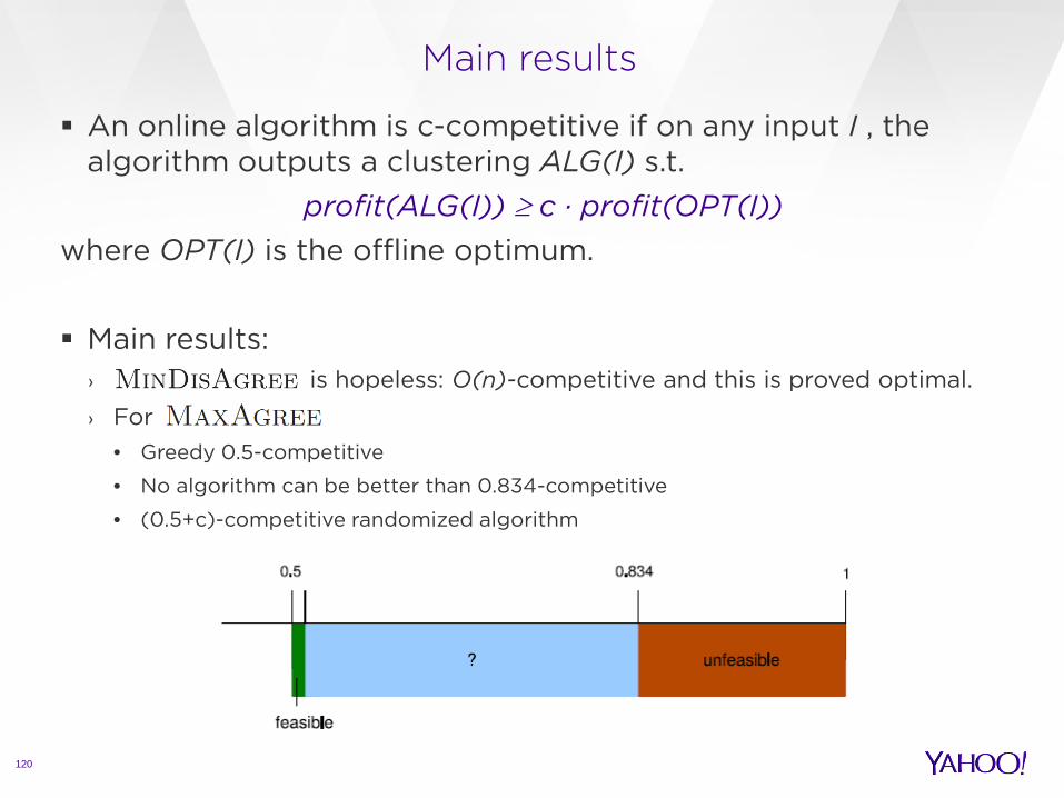
An online algorithm is c-competitive if on any input I , the algorithm outputs a clustering ALG(I) s.t.
profit(ALG(I)) ≥ c · profit(OPT(I)) where OPT(I) is the offline optimum. Main results:
› is hopeless: O(n)-competitive and this is proved optimal.
› For • Greedy 0.5-competitive
• No algorithm can be better than 0.834-competitive
• (0.5+c)-competitive randomized algorithm

Bipartite correlation clustering
121
N. Ailon, N. Avigdor-Elgrabli, E. Liberty, A. van Zuylen Improved Approximation Algorithms for Bipartite Correlation Clustering
ESA 2011

Correlation bi-clustering

Correlation bi-clustering
Users – Items Raters – Movies B-cookies – User_Id Web Queries - URLs

Input for correlation bi-clustering
124
The input is an undirected unweighted bipartite graph.

Output of correlation bi-clustering
125
The output is a set of bi-clusters.
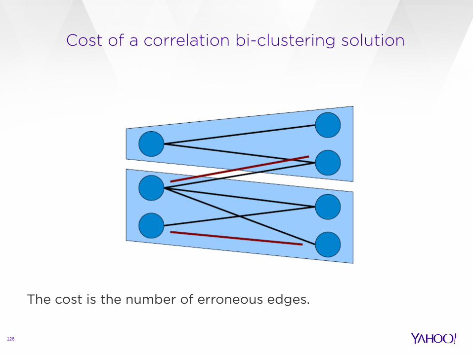
Cost of a correlation bi-clustering solution
126
The cost is the number of erroneous edges.

PivotBiCluster
127

PivotBiCluster
128

PivotBiCluster
129

PivotBiCluster
130

PivotBiCluster
131
PivotBiCluster
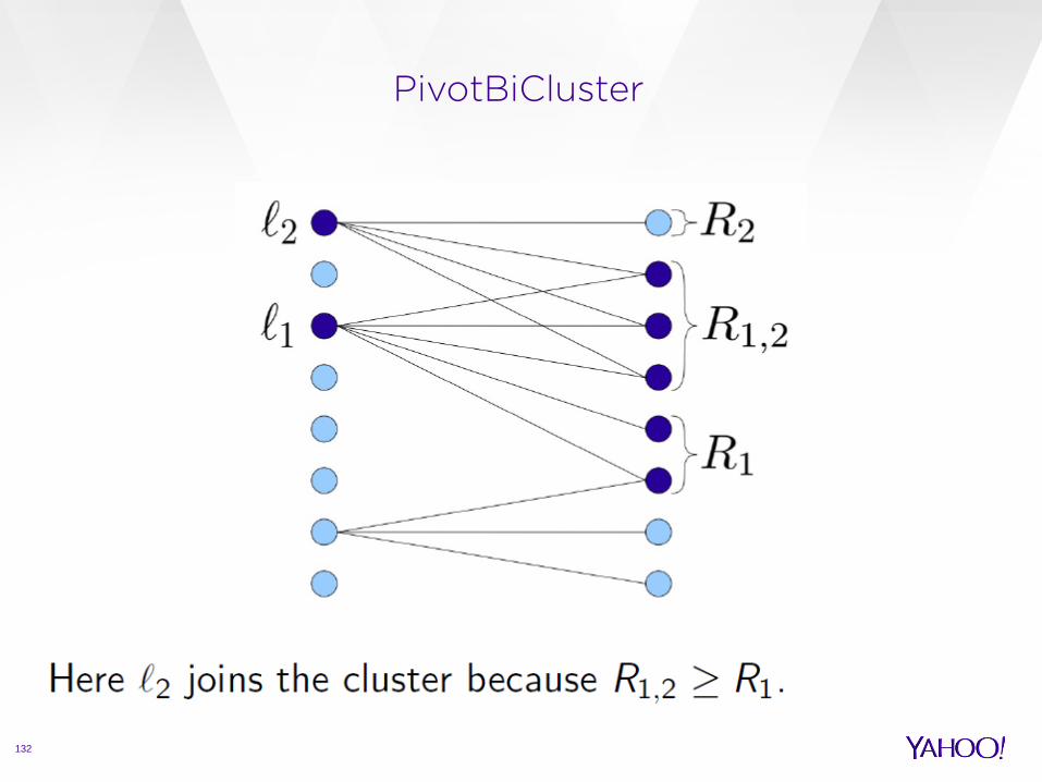
132

PivotBiCluster
133

PivotBiCluster
134
PivotBiCluster
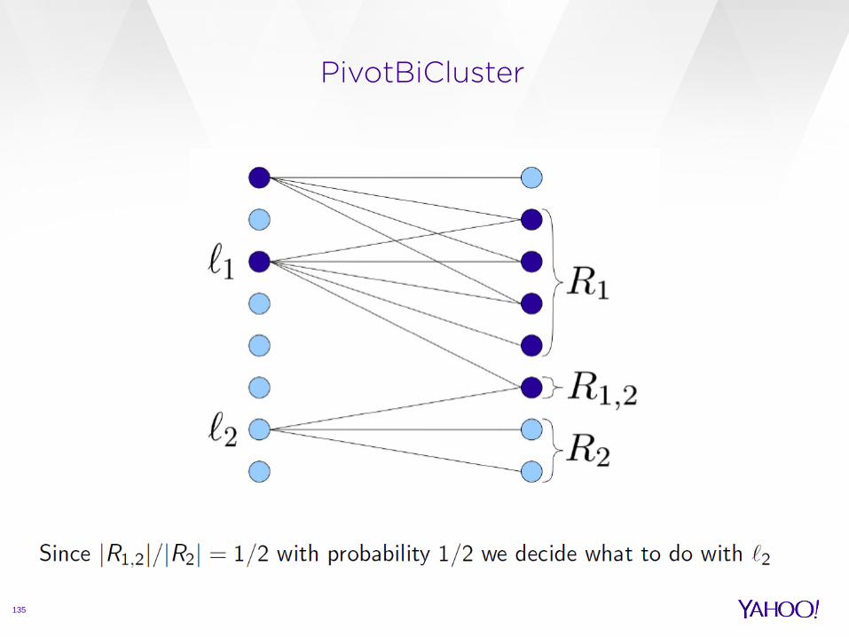
135

PivotBiCluster
136

PivotBiCluster
137
PivotBiCluster
138
Let OPT denote the best possible bi-clustring of G. Let B be a random output of PivotBiCluster. Then:
E[cost(B)] ≤ 4cost(OPT)
Let's see how to prove this...

Tuples, bad events, and violated pairs
139
Tuples, bad events, and violated pairs
140

Tuples, bad events, and violated pairs
141
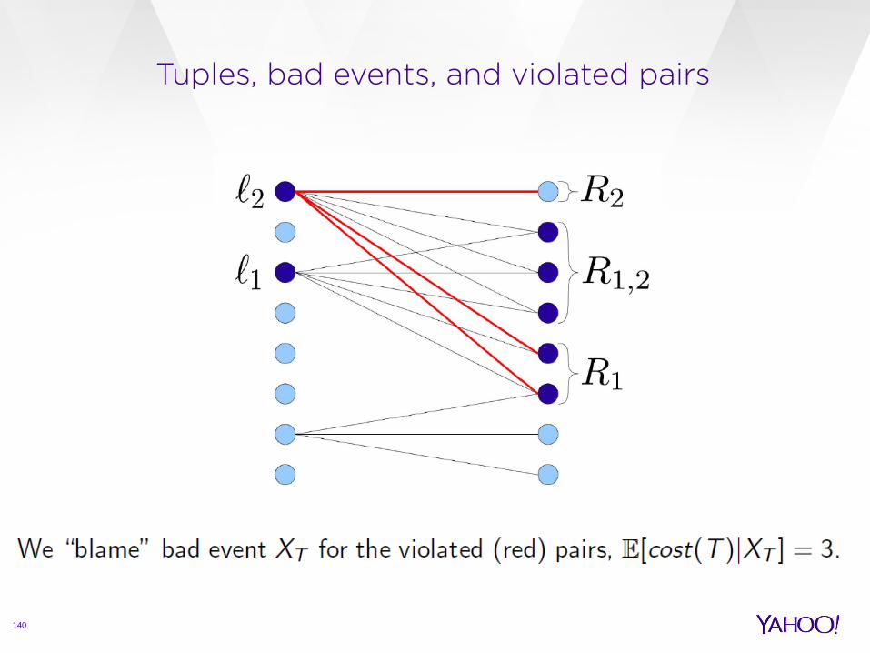
Since every violated pair can be blamed on (or colored by) one bad event happening we have:
where qT denotes the probability that a bad event happened to tuple T.
Note: the number of tuples is exponential in the size of the graph.

Proof sketch
142

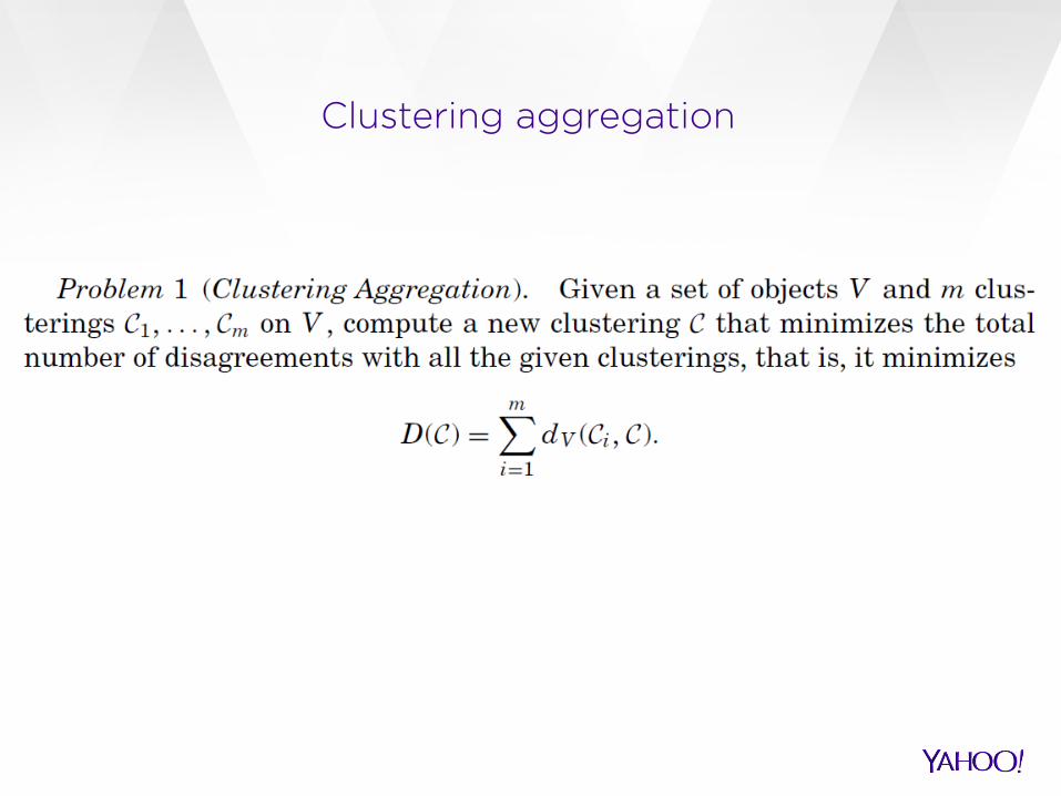
Clustering aggregation
143
A. Gionis, H. Mannila, P. Tsaparas Clustering aggregation ICDE 2004 & TKDD

Clustering aggregation
Many different clusterings for the same dataset! › Different objective functions › Different algorithms › Different number of clusters
Which clustering is the best?
› Aggregation: we do not need to decide, but rather find a reconciliation between different outputs

The clustering-aggregation problem
Input › n objects V = v1,v2,…,vn › m clusterings of the objects C1,…,Cm
Output › a single partition C, that is as close as possible to all input
partitions
How do we measure closeness of clusterings? › disagreement distance

Disagreement distance
U C P
x1 1 1
x2 1 2
x3 2 1
x4 3 3
x5 3 4
d(C,P) = 3
Clustering aggregation

Why clustering aggregation?
Clustering categorical data
The two problems are equivalent
U City Profession Nationality
x1 New York Doctor U.S.
x2 New York Teacher Canada
x3 Boston Doctor U.S.
x4 Boston Teacher Canada
x5 Los Angeles Lawer Mexican
x6 Los Angeles Actor Mexican
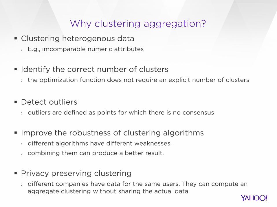
Why clustering aggregation? Clustering heterogenous data
› E.g., imcomparable numeric attributes
Identify the correct number of clusters › the optimization function does not require an explicit number of clusters
Detect outliers
› outliers are defined as points for which there is no consensus
Improve the robustness of clustering algorithms › different algorithms have different weaknesses.
› combining them can produce a better result.
Privacy preserving clustering › different companies have data for the same users. They can compute an
aggregate clustering without sharing the actual data.
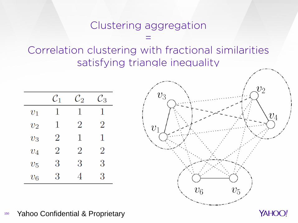
Clustering aggregation =
Correlation clustering with fractional similarities satisfying triangle inequality
150 Yahoo Confidential & Proprietary

Metric property for disagreement distance
d(C,C) = 0 d(C,C’)≥0 for every pair of clusterings C, C’ d(C,C’) = d(C’,C) Triangle inequality? It is sufficient to show that for each pair of points x,y
єV: dx,y(C1,C3)≤ dx,y(C1,C2) + dx,y(C2,C3)
dx,y takes values 0/1; triangle inequality can only be violated when
dx,y(C1,C3) = 1 and dx,y(C1,C2)= 0 and dx,y(C2,C3) = 0 › Is this possible?
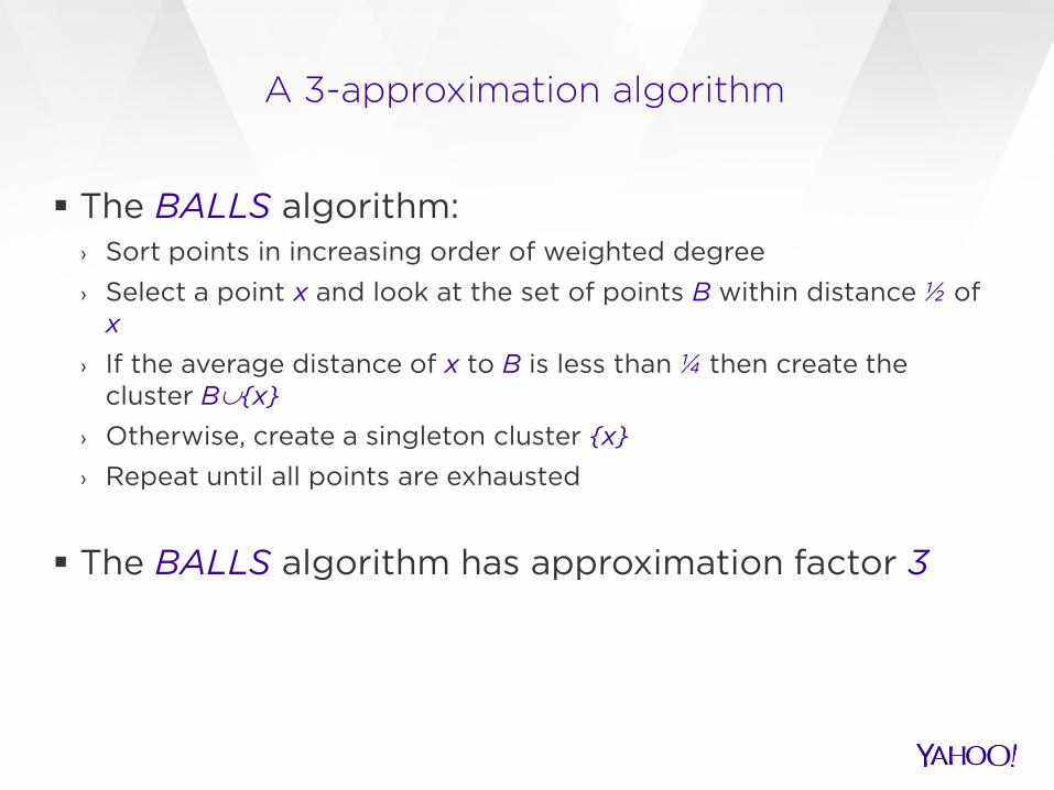
A 3-approximation algorithm
The BALLS algorithm: › Sort points in increasing order of weighted degree › Select a point x and look at the set of points B within distance ½ of
x › If the average distance of x to B is less than ¼ then create the
cluster B∪x › Otherwise, create a singleton cluster x › Repeat until all points are exhausted
The BALLS algorithm has approximation factor 3

Other algorithms
153
Picking the best clustering among the input clusterings, provides 2(1-1/m) approximation ratio. › However, the runtime is O(m^2n)
Ailon et al. (STOC 2005) propose a similar pivot-like algorithm
(for correlation clustering) that for the case of similarity satisfying triangle inequality gives an approximation ratio of 2.
For the specific case of clustering aggregation they show that chosing the best solution between their algorithm and the best of the input clusterings, yelds a solution with expected approximation ratio of 11/7.

Part I I I : Scalabi l ity for real-world instances
154
David Garcia-Soriano Yahoo Labs, Barcelona

Application 1: B-cookie de-duplication
SID = Andre
SID = Steffi
B = A work
B = A laptop
B = AS home
B = S work
Each visit to Yahoo sites is tied to a browser B-cookie. We also know the hashed Yahoo IDs (SIDs) of users who are logged in. Many-many relationship between B-cookies and SIDs.
ProblemHow to identify the set of distinct users and/or machines?

Application 1: B-cookie de-duplication (II)
Data for a few days may occupy tens of Gbs and contain hundreds ofmillions of cookies/SIDs.
It is stored across multiple machines.
We have developed a general distributed and scalable framework forcorrelation clustering in Hadoop.
The problem may be modeled as correlation bi-clustering, but we chooseto use standard CC for scalability reasons.
Application 1: B-cookie de-duplication (II)
Data for a few days may occupy tens of Gbs and contain hundreds ofmillions of cookies/SIDs.
It is stored across multiple machines. We have developed a general distributed and scalable framework for
correlation clustering in Hadoop. The problem may be modeled as correlation bi-clustering, but we choose
to use standard CC for scalability reasons.
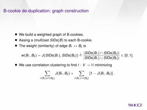
B-cookie de-duplication: graph construction
We build a weighted graph of B-cookies. Assing a (multi)set SIDs(B) to each B-cookie. The weight (similarity) of edge B1 ↔ B2 is
w(B1,B2) = J(SIDs(B1),SIDs(B2)) ,|SIDs(B1) ∩ SIDs(B2)||SIDs(B1) ∪ SIDs(B2)| ∈ [0, 1].
We use correlation clustering to find ` : V → N minimizing∑`(B1) 6=`(B2)
J(B1,B2) +∑
`(B1)=`(B2)
[1− J(B1,B2)] .

Application 2 (under development): Yahoo Mail
Spam detection
Spammers tend to send groups of groups emails very similar contents. Correlation clustering can be applied to detect them.

How is the graph given?
How fast we can perform correlation clustering depends on how the edgeinformation is accessed.For simplicity we describe the case of 0-1 weights.
1. Neighborhood oracles: given v ∈ V , return its positive neighbours:
E+(v) = w ∈ V | (v ,w) ∈ E+.
2. Pairwise queries: given a pair v ,w ∈ V , determine if (v ,w) ∈ E+.

Part 1 : CC wi th ne ighborhood orac les
1
Constructing neighborhood oracles
Easy if the input is the graph of positive edges explicitly given. Otherwise, locality sensitive hashing may be used for certain distance
metrics such as Jaccard similarity. This technique involves computing a set Hv of hashes for each node v
based on its features, and building an inverted index. Given a node v , we can retrieve the nodes whose similarity with v
exceeds a certain threshold by inspecting the nodes w withH(w) ∩H(v) 6= ∅.
Large-scale correlation clustering with neighborhood oracles
We show a system that achieves an expected 3-approximationguarantee with a small number of MapReduce rounds.
A different approach with high-probability bounds has been developed byChierichetti, Dalvi and Kumar: Correlation Clustering in MapReduce,KDD’14 (Monday 25th, 2pm).
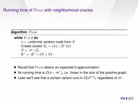
Running time of Pivot with neighborhood oracles
Algorithm Pivot
while V 6= ∅ dov ← uniformly random node from VCreate cluster Cv = v ∪ E+(v)V ← V \ Cv
E+ ← E+ ∩ (V × V )
Recall that Pivot attains an expected 3-approximation. Its running time is O(n + m+), i.e., linear in the size of the positive graph. Later we’ll see that a certain variant runs in O(n3/2), regardless of m+.
Running time of Pivot (II)
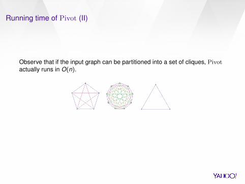
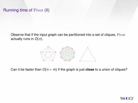
Observe that if the input graph can be partitioned into a set of cliques, Pivotactually runs in O(n).
Can it be faster than O(n + m) if the graph is just close to a union of cliques?
Running time of Pivot (II)
Observe that if the input graph can be partitioned into a set of cliques, Pivotactually runs in O(n).
Can it be faster than O(n + m) if the graph is just close to a union of cliques?
Running time of Pivot (III)
Theorem (Ailon and Liberty, ICALP’09)The expected running time of Pivot with a neighborhood oracle isO(n + OPT ), where OPT is the cost of the optimal solution.
Proof: Each edge from a center either captures a cluster element or disagrees
with the final clustering C. There are at most n− 1 edges of the first type, and cost(C) ≤ 3 ·OPT of
the second.

So where’s the catch?
The algorithm needs Ω(n) memory to store the set of pivots found so far(including singleton clusters.)
It is inherently sequential (needs to check if the new candidate pivot hasconnections to previous ones).
We would like to be able to create many clusters in parallel.

Running Pivot in parallel
Observation #1: after fixing a random vertex permutation π, Pivot becomesdeterministic.
Algorithm Pivot
π ← random permutation of Vfor v ∈ V by order of π do
if v is smaller than all of E+(v) according to π thenCreate cluster Cv = v ∪ E+(v) # v is a center, E+(v) are spokesV ← V \ Cv
E+ ← E+ ∩ (V × V )
Observation #2: If a vertex comes before all its neighbours (in the orderdefined by π), it is a cluster center. We can find them in parallel in one round.
Observation #3: We should remove remove edges as soon as possible, i.e.,when we know for sure whether or not a vertex is a cluster center.
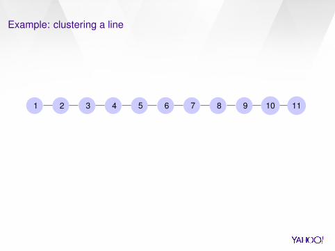
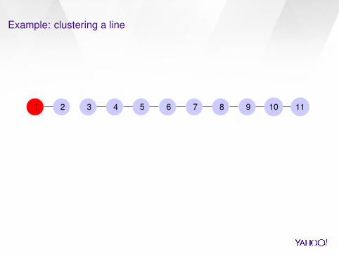
Example: clustering a line
1 2 3 4 5 6 7 8 9 10 11
11 31 3 51 3 5 71 3 5 7 91 3 5 7 9 11
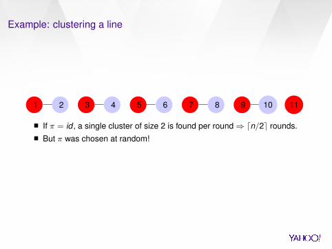
If π = id , a single cluster of size 2 is found per round⇒ dn/2e rounds.
But π was chosen at random!
Example: clustering a line
1 2 3 4 5 6 7 8 9 10 111
1 31 3 51 3 5 71 3 5 7 91 3 5 7 9 11
If π = id , a single cluster of size 2 is found per round⇒ dn/2e rounds. But π was chosen at random!

Example: clustering a line
1 2 3 4 5 6 7 8 9 10 11
1
1 3
1 3 51 3 5 71 3 5 7 91 3 5 7 9 11
If π = id , a single cluster of size 2 is found per round⇒ dn/2e rounds. But π was chosen at random!

Example: clustering a line
1 2 3 4 5 6 7 8 9 10 11
11 3
1 3 5
1 3 5 71 3 5 7 91 3 5 7 9 11
If π = id , a single cluster of size 2 is found per round⇒ dn/2e rounds. But π was chosen at random!

Example: clustering a line
1 2 3 4 5 6 7 8 9 10 11
11 31 3 5
1 3 5 7
1 3 5 7 91 3 5 7 9 11
If π = id , a single cluster of size 2 is found per round⇒ dn/2e rounds. But π was chosen at random!

Example: clustering a line
1 2 3 4 5 6 7 8 9 10 11
11 31 3 51 3 5 7
1 3 5 7 9
1 3 5 7 9 11
If π = id , a single cluster of size 2 is found per round⇒ dn/2e rounds. But π was chosen at random!

Example: clustering a line
1 2 3 4 5 6 7 8 9 10 11
11 31 3 51 3 5 71 3 5 7 9
1 3 5 7 9 11
If π = id , a single cluster of size 2 is found per round⇒ dn/2e rounds. But π was chosen at random!
Example: clustering a line
1 2 3 4 5 6 7 8 9 10 11
11 31 3 51 3 5 71 3 5 7 9
1 3 5 7 9 11
If π = id , a single cluster of size 2 is found per round⇒ dn/2e rounds. But π was chosen at random!

Clustering a line: random permutation
2 5 4 9 1 8 3 6 7 11 10
2 5 9 112 5 9 114 1 8 3 6 102 5 9 1174 1 8 3 6 10

Clustering a line: random permutation
2 5 4 9 1 8 3 6 7 11 102 5 9 11
2 5 9 114 1 8 3 6 102 5 9 1174 1 8 3 6 10
Clustering a line: random permutation
2 5 4 9 1 8 3 6 7 11 10
2 5 9 11
2 5 9 114 1 8 3 6 10
2 5 9 1174 1 8 3 6 10

Clustering a line: random permutation
2 5 4 9 1 8 3 6 7 11 10
2 5 9 112 5 9 114 1 8 3 6 10
2 5 9 1174 1 8 3 6 10

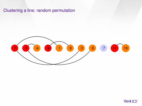
Clustering a line: random permutation (II)
Some intuition: For a line, we expect to find 1/3 of the vertices to be pivots in the first
round. The ”longest dependency chain“ has expected size O(log n). Thus we expect to cluster the line in about log n rounds.

Pseudocode for ParallelPivot
Pick a random bijection π : V → |V | # π encodes a random vertex permutationC = ∅ # C is the set of vertices known to be cluster centersS = ∅ # S is the set of vertices known not to be cluster centersE = E+ ∩ (i, j) | π(i) < π(j) # Only keep “+” edges respecting the permutation orderwhile C ∪ S 6= V do
# For each round, pick pivots in parallel and update C, S and E .for i ∈ V \ (C ∪ S) do
# i ’s status is unknownN(i) = j ∈ V | (i, j) ∈ E # Remaining neighbourhood of iif N(i) = ∅ then
# i has no smaller neighbour left; it is a cluster center.# Also, none of the remaining neighbours of i is a center (but they may be assigned to another center).C = C ∪ iS = S ∪ N(i)E = E \ E(i ∪ N(i))
Each vertex can be a cluster center or a spoke (attached to a center). When a vertex finds out about its own status, it notifies its neighbours. Otherwise it asks about the status of the neighbours it needs to know.

ParallelPivot: analysis
We obtain the exact same clustering that Pivot would find for a given vertexpermutation π. Hence the same approximation guarantees hold.
The i th round (iteration of the while loop) requires O(n + mi ) work, wheremi = |E+| is the number of edges remaining (which is strictly decreasing).
Question: How many rounds before termination?

Pivot and Maximal Independent Sets (MISs)
Focus on the set of cluster centers found:
Algorithm Pivot
π ← random permutation of VC ← ∅for v ∈ V in order of π do
if v has no earlier neighbours in C thenC ← C ∪ vCv = v ∪ E+(v) # v is a center, E+(v) are spokesV ← V \ Cv
C is an independent set: there are no edges between two centers. It is also maximal: cannot be extended by adding more vertices to C. Finding set of pivots ≡ finding a lexicographically smallest MIS (after
applying π).

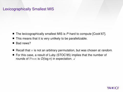
Lexicographically Smallest MIS
The lexicographically smallest MIS is P-hard to compute [Cook’67]. This means that it is very unlikely to be parallelizable. Bad news?
Recall that π is not an arbitrary permutation, but was chosen at random. For this case, a result of Luby (STOC’85) implies that the number of
rounds of Pivot is O(log n) in expectation. X

MapReduce implementation details
Each round of ParallelPivot uses two MapReduce jobs. Each vertex uses key-value pairs to send messages to its neighbours
whenever it discovers that it is/isn’t a cluster center. These two rounds do not need to be separated.

B-cookie de-duplication: some figures
We take data for a few weeks. The graph can be built in 3 hours. Our system computes a high-quality clustering in 25 minutes, after 12
Map-Reduce rounds. The average number of erroneous edges per vertex (in the CC measure)
is less than 0.2. The maximum cluster size is 68 and the average size among
non-singletons is 2.89. For a complete evaluation we wold need some ground truth data.

Part 2: CC wi th pa i rwise quer ies
2

Correlation clustering with pairwise queries
Pairwise queries are useful when we don’t have an explicit input graph.
ProblemMaking all
(n2
)pairwise queries may be too costly to compute or store.
Can we get approximate solutions with fewer queries?
Constant-factor approximations require Ω(n2) pairwise queries...

Query complexity/accuracy tradeoff
TheoremWith a “budget” of q queries, we can find a clustering C withcost(C) ≤ 3 ·OPT + n2
q in time O(nq).
This is nearly optimal.
We call this a (3, ε) approximation (where ε = 1q ).
Restating, we can find a (3, ε)-approximtion in time O(n/ε). This allows to find good clusterings up to a fixed an accuracy threshold ε. We can use this result about pairwise queries to give a faster
O(1)-approximation algorithm for neighborhood queries that runs inO(n3/2).
This result is a consequence of the existence of local algorithms forcorrelation clustering.
Bonchi, Garcıa-Soriano, Kutzkov: Local correlation clustering,arXiv:1312.5105.

Local correlation clustering (LCC)
DefinitionA clustering algorithm A is said to be local with time complexity t if havingoracle access to any graph G, and taking as input |V (G)| and a vertexv ∈ V (G), A returns a cluster label AG(v) in time O(t). Algorithm A implicitlydefines a clustering, described by the labelling `(v) = AG(v).
Each vertex queries t edges. Outputs a label identifying its own cluster in time O(t).
LCC → explicit clustering
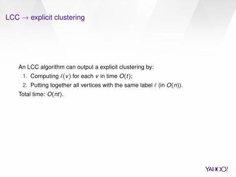
An LCC algorithm can output a explicit clustering by:
1. Computing `(v) for each v in time O(t);
2. Putting together all vertices with the same label ` (in O(n)).
Total time: O(nt).
In fact we can use LCC to cluster the part of the graph we’re interested inwithout having to cluster the whole graph.

LCC → explicit clustering
An LCC algorithm can output a explicit clustering by:
1. Computing `(v) for each v in time O(t);
2. Putting together all vertices with the same label ` (in O(n)).
Total time: O(nt).In fact we can use LCC to cluster the part of the graph we’re interested inwithout having to cluster the whole graph.

LCC → Local clustering reconstruction
Queries of the form “are x , y in the same cluster”? can be answered in timeO(t).
How: compute `(x) and `(y) in O(t), and check for equality. No need to partition the whole graph! This is is like “correcting” the missing/extraneous edges in the input data
on the fly. It fits into the paradigm of “property-preserving data reconstruction”
(Ailon, Chazelle, Seshadhri, Liu’08).

LCC → Distributed clustering
The computation can be distributed:
1. We can assign vertices to diffent processors.
2. Each processor computes `(v) in time O(t).
3. All processors must share the same source of randomness.

LCC → Streaming clustering
Edge streaming model: edges arrive in arbitrary order.
1. For a fixed random seed, the set of v ′s neighbours the LCC can queryhas size at most 2t .
2. This set can be compute before any edge arrives.
3. We only need to store O(n · 2t ) edges (this can be improved further.)
This has applications in clustering dynamic graphs.
LCC → Quick cluster edit distance estimators
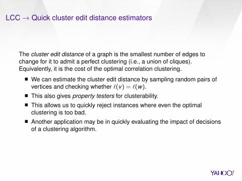
The cluster edit distance of a graph is the smallest number of edges tochange for it to admit a perfect clustering (i.e., a union of cliques).Equivalently, it is the cost of the optimal correlation clustering.
We can estimate the cluster edit distance by sampling random pairs ofvertices and checking whether `(v) = `(w).
This also gives property testers for clusterability. This allows us to quickly reject instances where even the optimal
clustering is too bad. Another application may be in quickly evaluating the impact of decisions
of a clustering algorithm.

Local correlation clustering: results
TheoremGiven ε ∈ (0, 1), a (3, ε)-approximate clustering can be found locally in timeO(1/ε) per vertex, (after O(1/ε2) preprocessing.) Moreover, finding an(O(1), ε)-approximation with constant success probability requires Ω(1/ε)queries.
This is particularly useful where the graph contains a relatively small numberof “dominant” clusters.

Local correlation clustering: algorithm
Algorithm LocalCluster(v , ε)
P ← FindGoodPivots(ε)return FindCluster(v ,P)
Algorithm FindCluster(v ,P)
if v /∈ E+(P) thenreturn v
elsei ← minj | v ∈ E+(Pj );
return Pi
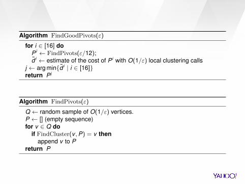
Algorithm FindGoodPivots(ε)
for i ∈ [16] doP i ← FindPivots(ε/12);d i ← estimate of the cost of P i with O(1/ε) local clustering calls
j ← arg mind i | i ∈ [16]return P j
Algorithm FindPivots(ε)
Q ← random sample of O(1/ε) vertices.P ← [] (empty sequence)for v ∈ Q do
if FindCluster(v ,P) = v thenappend v to P
return P

Part IV: Chal lenges and directions
for future research
155
Edo Liberty Yahoo Labs, NYC
Future challenges
157
Can we have efficient algorithms for weighted or partial graphs with provable approximation guaranties?
In practice, greedy algorithms work very well but provably fail sometimes. Can we characterize when that happens?
Practically solving Correlation Clustering problems in large scale is still a challenge.
Better conversion and representation of data as graphs will enable fast and efficient clustering.
Can we develop machine learned pairwise similarities that can support neighborhood queries over sets of objects?

158
Thank you! Questions?


![Chapter 01: Introducing Continuous Delivery - Packt · PDF fileChapter 08: Clustering with ... Chapter 09: Advanced Continuous Delivery [ ] [ ] [ ] [ ] YAHOO! change time flickr](https://img.dokumen.tips/doc/110x75/5a6fb5937f8b9abb538b5140/chapter-01-introducing-continuous-delivery-packt-nbsppdf-filechapter.jpg)