Correlated Failures of Power Systems:

Analysis of the Nordic Grid

MARTIN ANDREASSON

Master's Degree Project

Stockholm, Sweden February 2011

XR-EE-RT 2011:006

Abstract

The emphasis of this master's thesis is modeling and simulation of failures in large-scale

power grids. The linear DC-model governing the active power ows is derived and dis-

cussed, and the optimal load shedding problem is introduced. Using Monte Carlo

simulations, we have analyzed the eects of correlations between failures of power lines

on the total system load shed. Correlations are introduced by a Bernoulli failure model

with its rst two ordinary moments given explicitly. The total system load shed is

determined by solving the optimal load shedding problem in a MATLAB environment

using YALMIP and the GLPK solver. We have introduced a Monte Carlo simula-

tion framework for sampling the statistics of the system load shed as a function of

stochastic network parameters, and provide explicit guarantees on the sampling accu-

racy. This framework has been applied to a 470 bus model of the Nordic power grid. It

has been found that increased correlations between Bernoulli failures of power lines can

dramatically increase the expected value as well as the variance of the system load shed.

Keywords: Power grid, Monte Carlo simulation, Nordic grid, Modeling.

Contents

1 Introduction 1

1.1 Previous work . . . . . . . . . . . . . . . . . . . . . . . . . . . . . . . . . 1

1.2 Overview of work . . . . . . . . . . . . . . . . . . . . . . . . . . . . . . . 4

1.3 Main contributions . . . . . . . . . . . . . . . . . . . . . . . . . . . . . . 4

2 Power ow analysis 6

2.1 Graph models for power networks . . . . . . . . . . . . . . . . . . . . . . 6

2.2 Power ow equations . . . . . . . . . . . . . . . . . . . . . . . . . . . . . 7

2.2.1 Nonlinear DC-model . . . . . . . . . . . . . . . . . . . . . . . . . 8

2.2.2 Linear DC-model . . . . . . . . . . . . . . . . . . . . . . . . . . . 8

2.2.3 Transmission constraints in power systems . . . . . . . . . . . . . 9

2.2.4 Transmission constraints under the linear DC-model . . . . . . . 10

2.3 Linear optimal load shedding . . . . . . . . . . . . . . . . . . . . . . . . 11

2.4 Switched optimal linear load shedding . . . . . . . . . . . . . . . . . . . 13

2.5 Power planning with uncertain demand and generation . . . . . . . . . . 16

3 Reliability of power systems 20

3.1 Deterministic reliability measures . . . . . . . . . . . . . . . . . . . . . . 20

3.1.1 N − k criterion . . . . . . . . . . . . . . . . . . . . . . . . . . . . 20

3.2 A probabilistic reliability measure . . . . . . . . . . . . . . . . . . . . . . 20

3.3 Monte Carlo methods for probabilistic reliability measures . . . . . . . . 23

3.3.1 Sampling Bernoulli line failures . . . . . . . . . . . . . . . . . . . 27

3.4 Sampling correlated Bernoulli failures . . . . . . . . . . . . . . . . . . . 27

4 The Nordic Power grid 30

4.1 Overview of the Nordic grid . . . . . . . . . . . . . . . . . . . . . . . . . 30

4.1.1 Market structure in the Nordic power grid . . . . . . . . . . . . . 30

4.1.2 Operation of the Nordic power network . . . . . . . . . . . . . . 31

4.1.3 Modernizations of the Nordic power grid . . . . . . . . . . . . . . 32

4.2 Reliability of the Nordic power grid . . . . . . . . . . . . . . . . . . . . . 33

i

4.3 Model of the Nordic power grid . . . . . . . . . . . . . . . . . . . . . . . 34

4.3.1 Collecting data of network topology . . . . . . . . . . . . . . . . 34

4.3.2 Collecting power generation data . . . . . . . . . . . . . . . . . . 35

4.3.3 Estimating power demand data . . . . . . . . . . . . . . . . . . . 35

4.3.4 Estimating line admittances . . . . . . . . . . . . . . . . . . . . . 38

4.3.5 Estimating line capacities . . . . . . . . . . . . . . . . . . . . . . 39

4.3.6 Evaluating the model . . . . . . . . . . . . . . . . . . . . . . . . 40

4.4 Simulations of correlated system failures in the Nordic power grid . . . . 41

4.4.1 Correlations between all power lines . . . . . . . . . . . . . . . . 42

4.4.2 Correlations between incident power lines . . . . . . . . . . . . . 45

4.4.3 Correlations between power lines incident to PMUs . . . . . . . . 49

4.5 Applications . . . . . . . . . . . . . . . . . . . . . . . . . . . . . . . . . . 52

4.5.1 Interactions between TSOs . . . . . . . . . . . . . . . . . . . . . 52

4.6 Discussion . . . . . . . . . . . . . . . . . . . . . . . . . . . . . . . . . . . 55

5 Conclusions and future research 57

Bibliography 58

A Notation 63

A.1 Mathematical notation . . . . . . . . . . . . . . . . . . . . . . . . . . . . 63

A.2 Denitions of terms . . . . . . . . . . . . . . . . . . . . . . . . . . . . . . 63

B Figures 65

C Mathematical preliminaries 68

C.1 Graphs . . . . . . . . . . . . . . . . . . . . . . . . . . . . . . . . . . . . . 68

C.1.1 Undirected graphs . . . . . . . . . . . . . . . . . . . . . . . . . . 68

C.1.2 Directed graphs . . . . . . . . . . . . . . . . . . . . . . . . . . . . 69

C.1.3 Weighted graphs . . . . . . . . . . . . . . . . . . . . . . . . . . . 69

C.1.4 Vertex degree . . . . . . . . . . . . . . . . . . . . . . . . . . . . . 69

C.2 Matrix representations of graphs . . . . . . . . . . . . . . . . . . . . . . 70

C.2.1 Vertex-edge incidence matrix . . . . . . . . . . . . . . . . . . . . 70

C.2.2 Laplacian . . . . . . . . . . . . . . . . . . . . . . . . . . . . . . . 71

C.3 Probability theory . . . . . . . . . . . . . . . . . . . . . . . . . . . . . . 73

C.3.1 Random variables . . . . . . . . . . . . . . . . . . . . . . . . . . . 73

C.3.2 Moments . . . . . . . . . . . . . . . . . . . . . . . . . . . . . . . 74

C.4 Linear programming . . . . . . . . . . . . . . . . . . . . . . . . . . . . . 75

C.4.1 Duality . . . . . . . . . . . . . . . . . . . . . . . . . . . . . . . . 76

C.5 Game theory . . . . . . . . . . . . . . . . . . . . . . . . . . . . . . . . . 76

C.5.1 Social optimum . . . . . . . . . . . . . . . . . . . . . . . . . . . . 77

ii

C.5.2 Pareto ecient solution . . . . . . . . . . . . . . . . . . . . . . . 77

C.5.3 Nash equilibrium . . . . . . . . . . . . . . . . . . . . . . . . . . . 77

C.6 Proofs . . . . . . . . . . . . . . . . . . . . . . . . . . . . . . . . . . . . . 78

C.6.1 Proof of proposition 2 . . . . . . . . . . . . . . . . . . . . . . . . 78

iii

Chapter 1

Introduction

1.1 Previous work

Power systems are among the largest and most complex systems created by mankind.

The complexity of power systems keeps increasing as power grids are expanded and new

functionalities are added, as with the development of the SmartGrid [Massoud and Wollenberg, 2005].

Because many vital parts of today's society require reliable supply of electricity, the

reliable and secure operation of power systems is essential [Amanullah et al., 2005,

Amin, 2002]. We give a brief overview of the research in the two distinctive areas of

security against adversarial attacks and reliability of power systems.

In the area of security, research on characterizing optimal attack and defense strate-

gies has gained momentum over the past years. [Salmeron et al., 2004] consider the

optimization problem of maximizing the power outage, for a given number of power

transmission lines that an adversary is capable of disconnecting. The system opera-

tor is assumed to take the best action to minimize the damage in form of compulsory

load shedding. The problem is by nature game theoretic and gives rise to a maximin

optimization problem, where the outer maximization seeks the most disruptive attack

for a given budget of the adversary, and the inner minimization solves the optimal

load shedding problem which minimizes the consequences of an attack. Because of the

non-convexity and the existence of integer variables, the problem is inherently hard to

solve for large systems. [Pinar et al., 2010] approximates the nonlinear mixed integer

bi-level program by a mixed integer linear program, and derive an upper bound on

the severity of adversarial attacks. [Arroyo and Galiana, 2005] considers a fairly more

general formulation of the terrorist threat problem, where the terrorist's and system

operator's objectives are not necessarily antagonistic. This is a natural extension of the

maximin optimization formulation, and the formulation leads to a bi-level optimization

program. The authors have considered the linear DC model, and thus the bi-level opti-

mization problem is linear. By replacing the inner optimization by it's KKT conditions

1

and rewriting them as linear inequalities, the problem is transformed into a single-level

mixed integer linear optimization program, which is solved by standard commercial

software.

Traditionally, the reliability of power systems has often been characterized by de-

terministic means, such as the widely uses N − k criterion [Billinton and Allan, 1995].

A power system satisfying the N − k criterion is able to withstand any contingency

consisting of k outages. The advantage with deterministic reliability criteria is that

rubustness is guaranteed explicitely, as with the N − k criterion. The main drawback

of deterministic reliability criteria however is that they do not take into account the

probabilities of contingencies. Furthermore the number of events which have to be con-

sidered grows exponentially in k, making the reliability evaluation computationally in-

tractable. More recent research on the reliability of power systems has emphasized that

many events governing the reliability of power systems are by nature stochastic, e.g.

demands and generation capacities. Various statistical and sampling based methods

for evaluating the reliability of power systems have been developed to analyze stochas-

tic phenomena in power systems [Roy Billinton, 1994, Allan and Billinton, 2000]. In

[Billinton and Wang, 1999] a two state Markov model for the failure of various power

system elements is considered, and the statistics of the power system are calculated

using Monte Carlo techniques. [Chertkov et al., 2010] considers the power demand

as a random variable, to determine the likelihood of the most common causes of

power shortage in a power system by a heuristic optimization algorithm. The pa-

per focuses on the linear DC model and assumes Gaussian demand distributions.

[Billinton and Khan, 1992] studies the reliability of a 5-bus power system by consider-

ing nearly all combinations of contingencies, and calculating the load shed needed to

restore the system to a secure operational state. The power system reliability is dened

by the likelihood of the discrete operational states of normal, restorative, alert, emer-

gency and extreme emergency respectively, as dened in the paper. The amount of load

shedding is determined by a linear program, by using the linearized DC-model. One

drawback with this approach is the dramatically increased complexity as the network

size increases. In [da Silva et al., 2004] the authors use a Monte Carlo simulation based

approach to quantify the reliability of a power system. Reliability here is quantied

by the states healthy, marginal and at risk. The proposed algorithm samples states

based on a probability distribution, after which optimal power dispatch is performed.

In [Anghel et al., 2007], the authors use Monte Carlo methods to model cascading fail-

ures and major blackouts of power grids. Their model covers random removal of system

components, as well as random load uctuations. The load uctuations are translated

into heat variations of the power transmission lines by the use of a heat diusion model,

which causes random failures of the power transmission lines. To capture the dynam-

ics of cascading failures, the system is simulated over a time period, and recoveries as

2

well as protective actions by the transmission operator (TO) are modeled. The algo-

rithms are applied to a 100-node power transmission system and examples of predicted

blackouts are demonstrated. Other than failure correlations due to cascading failures

[Kinney et al., 2005], we found no model which attempts to model correlated failures

in power systems.

The Monte Carlo techniques in this work rely on the deterministic operation of op-

timal load shedding in power systems. Optimal load shedding for system protection is a

form of an optimal power ow problem and is a classical problem in the power systems

community. For a survey of studied problems see e.g. [Huneault and Galiana, 1991].

The optimal load shedding problem is a system protection measure to, in some mean-

ingful sense, optimally dispatch power in the network to avoid system faults. The

classical formulations of the optimal load shedding problem consider a static network,

where the decision variables are the phase angles of the nodes in the power network, and

the objective is a (weighted) sum of power decits in the nodes. [Fisher et al., 2008]

consider a more general formulation of the optimal load shedding problem for system

protection, where they take into account the switching of power transmission lines,

so called optimal transmission switching (OTS). The binary variables associated with

the on-o state of each power line together with the linearized power ow model, give

rise to a mixed integer linear program, which may be solved by standard commercial

software.

The OTS can be generalized by considering the use of exible AC transmission sys-

tems (FACTS). FACTS is a collection of technologies used to control the AC power ows

in transmission lines. The power ow through the power network is determined solely by

the phase angles and voltages of the buses, and the power transmission line admittances.

See e.g. [Abur and Exposito, 2004] for a review of the Kircho voltage law (KVL) and

the power ow equations. Due to the KVL there are no direct ways of routing electricity,

as with e.g. trac ows, and hence the control of power transmission networks is fairly

inexible. FACTS technologies however, open the possibility to control the line admit-

tances in close to real time, allowing to control the power ow from the nodes, without

changing the phase angles of any other nodes. The line admittances in FACTS are con-

trolled by changing adjustable inductors and capacitors installed in the transmission

lines. The FACTS and applications to power network control technologies are described

more in detail in [Hingorani, 1993, Gotham and Heydt, 1998, Xiao et al., 2002]. At-

tempts to incorporate FACTS devices in existing optimal power dispatch models have

been made in [Preedavichit and Srivastava, 1998, Lu and Abur, 2002].

3

1.2 Overview of work

This work aims at studying the eects of increasing correlations between failures of

power system components. In contrast to previous papers on the subject, we introduce

a failure model which explicitly takes into account correlated failures. In particular, we

consider a Bernoulli model of correlated power line failures. We measure the impact of

correlations of failures by the covariances between the failures.

Many of the SCADA systems used in controlling power systems are running general-

purpose operating systems, e.g. Microsoft Windows based operating systems and

general-purpose software. This makes SCADA systems vulnerable to software bugs

within the operating system and control applications. When identical software is de-

ployed in several system components, software failures are likely to be more correlated

between these components. We feel that the eects of correlated failures of power sys-

tems have not been adequately studied, although there is reason to believe that many

failures in power systems could be correlated. In this work, we measure the impact of

a system failure by the minimum system load shed required to restore the system to a

safe state. This formulation gives rise to an optimization problem, which under some

conditions can be made linear. For dierent values of the correlations of the failure

distribution, we compute the sampled statistics of the total system load shed by Monte

Carlo techniques, and provide guarantees on the convergence rate of the sampled statis-

tics. In particular, we use a weighted sum of the mean and variance of the total system

load shed as a risk measure of the failure statistics. To obtain statistical data from

a realistic power system, we apply our techniques to a 470 bus model of the Nordic

power system, acquired from publicly available sources. Certain information of the

Nordic power grid are available and can be put together to build a full model, whereas

other information is unavailable and needs to be estimated. Applying the Monte Carlo

simulation techniques to the Nordic grid model, we have found that increasing corre-

lations between Bernoulli failures of power lines lead to increased expected value and

variance of the system load shed.

1.3 Main contributions

This work presents a novel model of the Nordic power grid, used for studying correlated

failures of power lines. While examples from the Nordic power grid have been used

widely in power systems research, we know of no full-scale publicly available model of

the Nordic power system for simulating static power ows.

Using the novel model of the Nordic grid, we have simulated correlated Bernoulli

failures of power lines. Besides the novelty of the model and problem formulation, we

have found that increased correlations lead to increased costs measured in the mean and

4

the variance of the system load shed. We furthermore show sucient conditions, for

when increasing correlations between Bernoulli failures of power lines lead to increased

expected system load shed and increased variance of the system load shed.

5

Chapter 2

Power ow analysis

2.1 Graph models for power networks

Denition 2.1. A weighted, directed graph is a set

G = (V,E) where E ∈ V × V

v ∈ V are called the vertices of, and e ∈ E are called the edges of the graph. The

number of vertices V and edges E are denoted |V | and |E|.

Denition 2.2. An edge eij going from vertex vi to vertex vj with weight wij is denoted

eij =(vi, vj , wij

)Denition 2.3. An graph is said to be unweighted if wij = 1 ∀ i, j : eij ∈ E, and

undirected if eij = eji ∀ i, j : eij ∈ E

Denition 2.4. The degree, deg(·) of a vertex is the number of edges connected to the

vertex.

Denition 2.5. The vertex-edge incidence matrix for a directed graph is dened as:

A = [Aij ] where Aij =

1 if ei = (vj , u) ∈ E−1 if ei = (u, vj) ∈ E

0 otherwise

for some node u ∈ V .

Denition 2.6. The weighted Laplacian is dened as

Lw = [lij ] where lij =

∑

j wij for i where vj is adjacent to vi if i = j

−wij if eij ∈ E−wji if eji ∈ E

0 otherwise

6

Theorem 1.

Lw = ATDwA (2.1)

where Dw = diag([wij ]).

For more details on graphs and for proofs, the reader is referred to Appendix C.1.

Denition 2.7. For power systems, the power buses, also referred to as nodes, are

modeled as vertices. The power transmission lines are modeled as edges.

2.2 Power ow equations

Power systems can be described using graph models, by letting the buses of the power

system be modeled as vertices, and the power transmission lines be modeled as edges

in the graph. We use the following notation for the power ow model:

Pij : Real power ow from bus i to j

Qij : Reactive power ow from bus i to j

P : Vector of total active power ow injected to the buses

Vi : Voltage of bus i

gij + jbij : Admittance of the series branch between bus i and j

gsj + jbsj : Admittance of the shunt branch at bus i

θi : Phase angle of bus i

θ : Vector of phase angles, θ = [θi]

θij = θi − θj : Phase angle dierence between bus i and j

From [Abur and Exposito, 2004] we obtain the nonlinear model for the real and reactive

power ow from bus i to bus j:

Pij = V 2i (gsi + gij)− ViVj(gij cos θij − bij sin θij) (2.2)

Qij = −V 2i (bsi + bij)− ViVj(gij sin θij − bij cos θij) (2.3)

By adding the incoming and subtracting the outgoing power ows into each node, we

obtain the equations for the real and reactive power injections for a node i.

Pi =∑

j:(ej ,ei)∈E

V 2i (gsi + gij)− ViVj(gij cos θij − bij sin θij)

−∑

j:(ei,ej)∈E

V 2i (gsi + gij)− ViVj(gij cos θij − bij sin θij) (2.4)

Qi =∑

j:(ej ,ei)∈E

−V 2i (bsi + bij)− ViVj(gij sin θij − bij cos θij

−∑

j:(ei,ej)∈E

−V 2i (bsi + bij)− ViVj(gij sin θij − bij cos θij) (2.5)

7

2.2.1 Nonlinear DC-model

Following [Pinar et al., 2010], we assume the resistance-to-reactance ratio to be suf-

ciently small. Furthermore we assume that the admittance in the shunt branch is

negligible. In (2.2)-(2.3) this translates to: gij = gsj = bsj = 0. Imposing these

approximations, we get the following power ow equations:

Pij = ViVjbij sin θij (2.6)

Qij = ViVjbij(cos θij − 1) (2.7)

Equations (2.6) - (2.7) are often referred to as the nonlinear DC-model. We may write

these equations in terms of power ow into the nodes, by using a graph model of the

power transmission network. Let the topology of the power transmission network be

given by the vertex-edge incidence matrix A. The line admittances are represented

as weights of the power transmission lines as B = diag(bij), and the node voltages as

V line = diag(ViVj

). The phase angles are represented as as Θ =

[θij]. It is easily seen

that Θ = Aθ, where θ is a vector of the absolute phase angles in the nodes and A is

the node art incidence matrix. Hence we can write:

P line = V lineB sin (Aθ) (2.8)

Qline = V lineB(cos (Aθ)− 1

)(2.9)

where P line =[Pij], Qline =

[Qij]and sin(x) =

[sin(xi)

], cos(x) =

[cos(xi)

]. Note

that V line is easily calculated once A is known, since the rows of A contain the infor-

mation of which nodes are connected.

2.2.2 Linear DC-model

For linearizing equations (2.6)- (2.7), we dene the following functions:

FP (θij |V, bij) = V linebij sin θij (2.10)

FQ(θij |V, bij) = V linebij(cos θij − 1) (2.11)

Linearizing (2.6)- (2.7) around θij = 0 ∀i, j, we obtain the following equations, valid

for suciently small values of θij :

Pij = FP (0|V, bij) + θij∂FP (θij |V, bij)

∂θij

∣∣∣∣∣θij=0

= V linebijθij (2.12)

Qij = FQ(0|V, bij) + θij∂FQ(θij |V, bij)

∂θij

∣∣∣∣∣θij=0

= 0 (2.13)

8

Equation (2.12) is commonly referred to as the linear DC model. As in the nonlinear

case, we may write equation (2.12) in vector form:

P line = V lineBAθ (2.14)

By adding the power ows to each node, we may write the power injections in the

nodes as:

P = ATV lineBAθ = LBθ (2.15)

where V = [Vi] Note that LB = ATV lineBA is analogue to the weighted Laplacian of

the power transmission network.

2.2.3 Transmission constraints in power systems

All power systems are endowed with hard physical transmission constraints, restricting

the active power ows. For simplicity but without loss of generality, we assume that

the nodes in the power system are partitioned into generator nodes, P g 0, and load

nodes, P l 0, i.e.

P =

[P g

P l

](2.16)

Line capacity constraints

Typically, there are physical capacity bounds on the power lines that take the form:

− P linemax P line P linemax (2.17)

Generation constraints

Each generator i has a maximum capacity P gmax,i, limiting the maximum power pro-

duction. Furthermore we assume that the minimum production for each generator is

0. Thus the constraints on the productions take the form

0 P g P gmax (2.18)

where 0 = [0, . . . , 0]T

Load constraints

We assume that each load node i has a predened demand, P ld,i. Furthermore we

assume that load nodes cannot be supplied with more power than the demand, and

that load nodes, per denition, cannot produce any power. Hence the load constraints

take the form

P ld P l 0 (2.19)

where P l are the actual loads of the nodes.

9

DC-model constraints

For the DC-model to be valid, the phase angle dierences must be suciently small.

By using the vertex-edge incidence matrix, this can be formulated as a single vector

constraint

−∆θmax · 1 Aθ ∆θmax · 1 (2.20)

where 1 = [1, . . . , 1]T , and 0 < ∆θmax ≤ π2 is a suciently small real number.

2.2.4 Transmission constraints under the linear DC-model

By using the linearized power ow equations (2.14)-(2.15), we can express P line, P l

and P g as linear functions of the phase angles θ. Furthermore, since all constraints

mentioned in section 2.2.3 are linear inequalities, we may write the intersection of all

constraints as a set of linear inequalities. Dene np as the number of power transmission

lines, ng and nl as the number of generator and load nodes respectively. Let n = ng+nlbe the total number of nodes. The feasibility constraints of equations (2.17)-(2.20) can

be written as

Cθ d (2.21)

where

C =

V lineBA

−V lineBA

LB−LBA

−A

d =

P linemax

P linemax

P gmax0nl×1

0ng×1

−P ld∆θmax · 1np×1

∆θmax · 1np×1

(2.22)

Denition 2.8. The feasible region of a power network is dened as

F =θ ∈ Rn |Cθ d

Denition 2.9. A state θ ∈ Rn is called feasible i

θ ∈ F

If a state θ is not feasible, it is called infeasible.

The power ow in a power transmission network is dependent on the topology of

the power network and load and generation data. We dene the conguration C of a

power system.

10

Denition 2.10. The conguration C of a power system is the set

C =V,A,B, P linemax, P

ld, P

gmax

Depending on the conguration C, it is either possible or not possible to satisfy all

power demands. We make the following denition to formalize the intuition.

Denition 2.11. A conguration C is called satisable i

∃θ ∈ F : HlLBθ = P ld

A conguration which is not satisable is called unsatisable.

2.3 Linear optimal load shedding

Recall that a conguration is satisable i there exists a feasible state such that all

load demands are satised. If a conguration is unsatisable, not all demands can be

met. In such cases, it is up to the transmission system operator (TSO) to cut the loads

for some load nodes. This procedure is called load shedding. When load shedding is

necessary, the TSO will try to minimize the total amount of load shedding needed to

restore the system to a feasible state. We dene the associated optimization problem,

called the optimal load shedding problem. It is easily veried that the corresponding

nonlinear optimal load shedding problem is in general non-convex, and hence inherently

hard to solve. For this reason, we will only consider the linear optimal load shedding

problem henceforth.

Denition 2.12. The linear optimal load shedding problem is dened as the linear

program

minθ

cT θ (2.23)

s.t. Cθ d

where

c =[01×ng 11×nl

]LB (2.24)

and c, C and d are as dened in equation (2.22). For a review of linear programming,

the reader is referred to appendix C.4.

The objective function ensures that the load of the demand nodes is minimized,

since the demand loads by denition are negative. The linear constraints represent

the constraints of the power system, discussed in 2.2.3. Given a disturbance of the

11

power system, which changes the conguration of the system, the resulting change to

the solution to (2.23) can be interpreted as a measure of how severe the disturbance is.

When no load shedding is necessary, this corresponds to normal operation of the power

system, while 100% load shed corresponds to a complete blackout where no power is

transmitted.

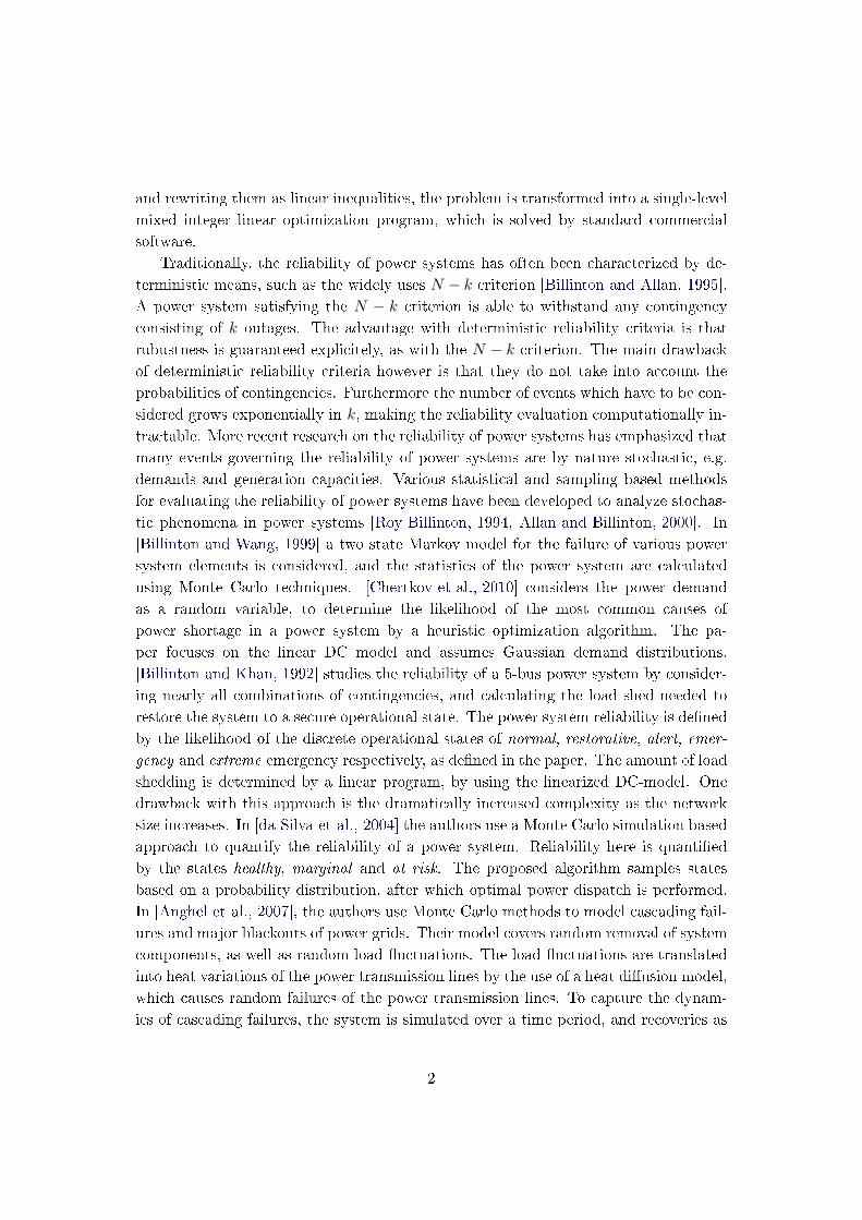
Example 2.3.1. Consider a 6-node and 7-line power transmission network, where

the nodes are partitioned into generator nodes (g1, g2), and load nodes (l1, l2, l3, l4)

For simplicity, we assume unit voltage V = 1 for all nodes. Given a power demand

g1

l1

l2

l3

l4

g2

l1

l2

l3l4

l5

l6l7

Figure 2.1: An example of a power network where the maximum line capacities are:

P linemax,1 = 1, P linemax,2 = 1, P linemax,3 = 1, P linemax,4 = 2, P linemax,5 = 1, P linemax,6 = 3, P linemax,7 = 3.

The line admittances are: b1 = 1, b2 = 1, b3 = 1, b4 = 1, b5 = 2, b6 = 2, b7 = 2. We

assume no generation capacity bounds

−P ld = [2, 2, 1, 1]T , the optimal power ow policy is given by the phase angles:

θ =

2.6436

1.6782

1.2055

0.5891

−0.2055

0.0000

(2.25)

12

and the power generations and ows are:

P g =

[2.8764

3.1236

]P line =

0.6164

0.7945

−0.2055

−1.2055

−0.9455

2.1782

2.8764

(2.26)

Since all demands are met, the system is feasible, i.e. load shedding is not necessary.

The value of the objective function is hence cT θ =∑P ld. The optimal power ow is

illustrated in gure 2.2.

g1

l1

l2

l3

l4

g2

0.6164

0.7945

0.2055

1.2055

0.9455

2.17822.8764

Figure 2.2: The optimal power ows shown graphically

2.4 Switched optimal linear load shedding

Example 2.4.1. Consider the following power transmission network.

13

g1

l1 l2

l1 l2

l3

Figure 2.3: A 3 node, 3 line power transmission network.

The generation capacity of g1 is 2, and the demands of l1 and l2 are both 2. The

transmission line capacities for the lines l1, l2 and l3 are 2, 2, 0.1 respectively, and

the line admittances are 1, 2, 1 respectively. The solution to the linear optimal load

shedding problem is illustrated in gure 2.4

g1

l1 l2

0.65 1.1

0.1

Figure 2.4: The optimal power ows shown graphically

Since node l1 only receives 0.75 but its demand is 1, the total load shed is 0.25.

Example 2.4.2. Now consider the same power transmission network as in example

2.4.1, but with line l3 cut o.

14

g1

l1 l2

l1 l2

Figure 2.5: A 3 node, 2 line power transmission network.

The solution to the linear optimal load shedding problem is illustrated in gure 2.6

g1

l1 l2

1 1

Figure 2.6: The optimal power ows shown graphically

Since both demands are satised, the total load shed is 0.

These preceding examples show that it may be benecial for the network operator to

switch o power transmission lines in order to reduce the system load shed. We dene

the associated optimization problem where it is possible to switch power transmission

lines on or o.

Denition 2.13. The switched optimal load shedding problem is dened as the mixed

integer program

minθ,Y

cT θ (2.27)

s.t. Csθ d

15

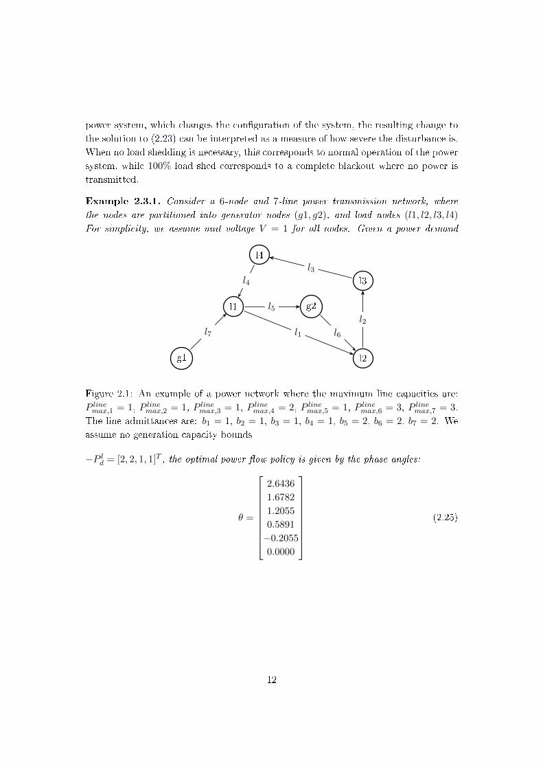
where c and d are as dened in equation (2.22), and

Cs =

V lineBY A

−V lineBY A

LSB−LSBA

−A

(2.28)

where

LSB = ATV lineBY A (2.29)

and

Y = diag([y1, . . . , ynp ]) where yi ∈ 0, 1 ∀i ∈ 1, . . . , np (2.30)

Lemma 2. The optimal value of the optimization program (2.27) is less than or equal

to the optimal value of the optimization program (2.23).

Proof. Assume, for the sake of contradiction, that the optimal solution of (2.23) is

strictly lower than the solution of (2.27). Clearly the optimizer for (2.23) is also a

feasible solution to (2.27), with Y = I. Thus, the optimal solution for (2.27) is at most

equal to the optimal solution of (2.23), contradicting the previous assumption.

Even though power line switching may be practically feasible for power transmission

networks, the switched optimal linear load shedding problem becomes computationally

hard as the number of transmission lines grows. Also, since the placement of new power

transmission lines is carefully considered before construction, it is unlikely that the

disconnection of some transmission line(s) will reduce the system load shed in practice.

Nevertheless, the switched optimal linear load shedding problem is a generalization of

the linear optimal load shedding problem and hence worth mentioning.

2.5 Power planning with uncertain demand and generation

Typically in most power grids, both demand and generation capacities vary over time,

and are not completely predictable. Demands usually vary depending on the time of

the day, the weather, season and other factors. Generation capacity is approximately

constant for traditional generators, such as gas turbines and nuclear power plants,

whereas the availability of many renewable generators such as water and wind power

exhibit major variations over time. By using their balancing controls, TSOs can take

real time actions to reschedule power ows when demand and generation uctuations

16

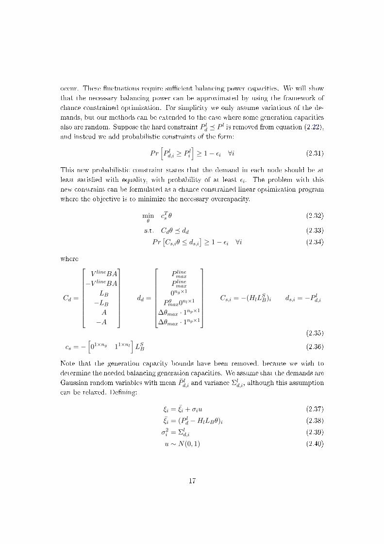
occur. These uctuations require sucient balancing power capacities. We will show

that the necessary balancing power can be approximated by using the framework of

chance constrained optimization. For simplicity we only assume variations of the de-

mands, but our methods can be extended to the case where some generation capacities

also are random. Suppose the hard constraint P ld P l is removed from equation (2.22),

and instead we add probabilistic constraints of the form:

Pr[P ld,i ≥ P li

]≥ 1− εi ∀i (2.31)

This new probabilistic constraint states that the demand in each node should be at

least satised with equality, with probability of at least εi. The problem with this

new constraint can be formulated as a chance constrained linear optimization program

where the objective is to minimize the necessary overcapacity.

minθ

cTs θ (2.32)

s.t. Cdθ dd (2.33)

Pr[Cs,iθ ≤ ds,i

]≥ 1− εi ∀i (2.34)

where

Cd =

V lineBA

−V lineBA

LB−LBA

−A

dd =

P linemax

P linemax

0ng×1

P gmax0nl×1

∆θmax · 1np×1

∆θmax · 1np×1

Cs,i = −(HlL

SB)i ds,i = −P ld,i

(2.35)

cs = −[01×ng 11×nl

]LSB (2.36)

Note that the generation capacity bounds have been removed, because we wish to

determine the needed balancing generation capacities. We assume that the demands are

Gaussian random variables with mean P ld,i and variance Σld,i, although this assumption

can be relaxed. Dening:

ξi = ξi + σiu (2.37)

ξi = (P ld −HlLBθ)i (2.38)

σ2i = Σl

d,i (2.39)

u ∼ N(0, 1) (2.40)

17

the probabilistic constraints in equation (2.34) can be written as

Pr [ξi ≤ 0] ≥ 1− εi ⇔ (2.41)

Pr

[u ≤ − ξi

σi

]≥ 1− εi ⇔ (2.42)

Erf

(− ξiσi

)≤ εi ⇔ (2.43)

Erf

−(P ld,i +HlLSBθ)i√

Σld,i

≤ εi ⇔ (2.44)

(HlLSBθ)i ≤ P ld,i + Erfinv(εi)

√Σld,i (2.45)

where

Erf(t) =1√2π

∫ t

−∞exp

(−x

2

2

)dx (2.46)

Erfinv(t) = Erf−1(t) (2.47)

Thus, the chance constrained LP in equation (2.32)-(2.34) becomes a standard LP:

minθ

cTs θ (2.48)

s.t. Ccθ dc (2.49)

where

C =

V lineBA

−V lineBA

HgLSB

−HgLSB

HlLSB

−(HlLSB)1

...

−(HlLSB)nl

A

−A

d =

P linemax

P linemax

P gmax0ng×1

0nl×1

−P ld,1 − Erfinv(ε1)√

Σld,1

...

−P ld,nl− Erfinv(εnl

)√

Σld,nl

∆θmax · 1np×1

∆θmax · 1np×1

(2.50)

and

Hg =[Ing×ng 0ng×nl

]Hl =

[0nl×ng Inl×nl

](2.51)

18

Note that if εi = 12 ∀i, i.e. we tolerate load shedding with probability 1

2 , this constraint

is equivalent to the demand constraints in equation (2.35). If however εi ≤ 12 , the

chance constraint will force the available load for the demand nodes to be higher than

the actual demand, to account for demand uctuations. Even though we have assumed

independence between the demands, it is not a particularly severe assumption. Since

the probability of load shedding should be less than εi for all demand nodes i, it also

handles the case where all demands are very close to the feasibility boundary. Still, a

solution to the optimal power ow problem as solved in section 2.3 is not guaranteed to

exist for all demands within the safe bounds, since the power ows are governed by the

Kircho voltage law (KVL). One would in theory have to solve a LP for every demand

to check feasibility for that demand. However, if the demands are perfectly correlated,

i.e.:

P ld,i = P ld + Σld,iu ∀i (2.52)

u ∼ N(0, 1) (2.53)

the convexity of the feasible polyhedron implies that all demands up to the critical

demand will allow for a solution of the optimal power ow problem.

Example 2.5.1. Consider the same power network as in example 2.3.1, with the only

dierence that the demands are now a random variable P ld ∼ N(P ld,Σld), with −P ld =

[1.2, 2, 0.5, 1]T and

Σld =

0.12 0 0 0

0 0.23 0 0

0 0 0.08 0

0 0 0 0.15

(2.54)

By applying the chance constrained optimization framework and letting ε = 0.05. The

power demands are

− P l =

1.346

2.203

0.6196

1.164

(2.55)

By solving (2.32), the total needed generation capacity is found to be

P g =

[2.5028

2.8296

](2.56)

The ratio between total generation capacity needed to meet unforeseen demand uctua-

tions and total power demand is 1.13.

19

Chapter 3

Reliability of power systems

3.1 Deterministic reliability measures

Traditionally the reliability of power systems has been evaluated by deterministic ro-

bustness measures. We will here describe the most widely used deterministic reliability

criterion, the N − k criterion.

3.1.1 N − k criterion

A widely adopted deterministic reliability measure in power transmission systems is

the N − k criterion.

Denition 3.1. Given a power transmission network and a discrete set N of com-

ponents with |N | = N , the power transmission network is said to satisfy the N − kcriterion if the conguration after the disconnection of any set of components Nl ⊆ Nwith |Nl| = l is satisable for l = 0, 1, . . . , k.

A commonly used special case of the N − k criterion is the case k = 1, in which

case the power transmission network should be satisable for all congurations where

a single component is disconnected. An advantage of the N − k criterion is that it

guarantees robustness against any number of k contingencies. However, it does not take

the probabilities of these contingencies into account, making it a rather conservative risk

measure. Furthermore the complexity of computing all k contingencies is exponential

in k, and quickly becomes infeasible for k > 1.

3.2 A probabilistic reliability measure

We here introduce a probabilistic risk measure of power systems based on the statis-

tical properties of the state of the power system. The risk measure will be based on

20

the amount of compulsory load shedding necessary to bring the system to a feasible

conguration. Recall the optimization problem given by (2.23). We dene the optimal

amount of load load shed as a function of the matrices C and d, characteristic for a

power system.

S∗(C, d) = minθ

cT θ|Cθ d

− 11×nl · P ld (3.1)

By introducing a probability measure on the topology of the power system, i.e. on the

matrices C and d, this corresponds to introducing a probability measure on the system

load shed. Indeed, the topology of the power system can be formalized by viewing the

matrices C and d as random variables endowed with the product probability measures

µC and µd, dened over the Lebesgue measurable spaces YC and Yd respectively.

Lemma 3. S∗(C, d) is continuous in C and d.

Proof. See e.g. [Bereanu, 1976] for a proof.

Lemma 4. S∗(C, d) is a random variable

Proof. Since S∗(C, d) is continuous in C and d, it is Borel measurable. Hence S∗(C, d)

is also a random variable endowed with a probability measure µS = µC × µd.

Thus, having shown that also S∗(C, d) is a random variable, we can dene operations

on the probability measure of S∗(C, d). Indeed, since 0 ≤ S∗(C, d) ≤ −P ld, the mean

and the variance of S∗(C, d) are bounded, and we can dene them as:

Denition 3.2. Given the random variables C and d with the product measure µS =

µC × µd , the expected load shed S∗ is dened as

S∗ =

∫Yc×Yd

S∗(C, d) dµs (3.2)

Denition 3.3. Given the random variables C and d with the product measure µS =

µS = µC×µd, and the expected load shed S∗, the variance of the load shed S∗ is dened

as

σ2S∗ =

∫Yc×Yd

(S∗(C, d)− S∗

)2dµs (3.3)

One can use the the rst two moments of the distribution of S∗(S, d) as a vector

valued risk measure. To be able to compare power systems of dierent size, one would

like to dene a risk measure that does not scale with the size of the power system,

like S∗ and σ2S∗ generally will. This can be achieved by normalizing S∗ and σ2

S∗ by

a scaling factor. Also, for comparisons between dierent distributions S∗(C, d), one

would rather have a scalar risk measure than a vector valued in some cases. Motivated

by this discussion, we here dene three dierent risk measures for power systems.

21

Denition 3.4. The absolute risk double Rabs is dened as

Rabs =[S∗, σS∗

]Denition 3.5. The relative risk double Rabs is dened as

Rrel =

[S∗

11×nl · P ld,

σS∗

11×nl · P ld

]

Denition 3.6. The weighted mean and standard deviation, WMSD, is dened as

S∗ + α · σS∗

where α ∈ R+ is a scaling factor of the standard deviation.

We will show that S∗+α·σS∗ is closely related to the value at risk (VaR) [Due and Pan, 1997].

Denition 3.7. VaRε(S∗) is dened as

VaRε(S∗) = infl ∈ R : Pr(S∗ > l) ≤ 1− ε

The intuitive meaning of VaRε(X) is that the probability of a loss greater than

VaRε(X) is less than or equal ε. Given the denition of VaR, we can state the following

proposition relating VaRα(X) to X and σ(X).

Proposition 1.

VaRα(X) ≤ X(X) +1√α· σ(X)

To prove the proposition, we need Chebyshev's inequality.

Lemma 5. (Chebyshev's inequality) Given any random variable X with mean X and

standard deviation σ

Pr(|X − X| ≥ α · σ) ≤ 1

α2

The proof now follows as a corollary of Chabyshev's inequality.

Proof. (of proposition 1) Note that

VaRα(X) ≤ X +1√ασ ⇔

Pr

(X < X +

1√α· σ)≥ 1− α

22

which is easily shown using Chebyshev's inequality

Pr

(X < X +

1√α· σ)≥

Pr

(∣∣X − X∣∣ < 1√α· σ)

=

1− Pr

(∣∣X − X∣∣ ≥ 1√α· σ)≥ 1− α

Thus the weighted sum of the mean and standard deviation of a random variable

X is an upper bound of the value at risk of the random variable X.

3.3 Monte Carlo methods for probabilistic reliability mea-

sures

To be be able to calculate the expected value and the variance of S∗(C, d) over the

probability measure µs, we will use a Monte Carlo sampling method. Formally, we

have the following problem.

S∗(C, d) = minθcT θ|Cθ d (3.4)

S∗(µs) =

∫Yc×Yd

S∗(C, d) dµs (3.5)

σ2S∗(µs) =

∫Yc×Yd

(S∗(C, d)− S∗

)2dµs (3.6)

In most applications, the event spaces are either continuous (in the case of continuously

varying demands), or very large (for example the total number of power line failures

is 2N , where N is the number of power lines). Since computing the expected loss S∗requires integrating over a continuous or at least intractably large set of solutions of a

LP, analytically computing the statistics of S∗(C, d) is practically infeasible. Instead,

we will use Monte Carlo methods to approximate equation (3.5)-(3.6) with the sampled

mean of S∗(C, d), built from a nite number of samples Ci and di of C and d. S∗(c,D)

and σS∗(µs) can be approximated by a nite number of samples by

S∗(µs) ≈ S∗,N (µs) =1

N

N∑i=1

S∗(Ci, di) (3.7)

σ2S∗(µs) ≈ σ2

S∗,N (µs) =1

N

N∑i=1

(S∗(Ci, di)− S∗,N (µs)

)2(3.8)

23

By (2.18) we have the following bounds on S∗(C, d) which will be useful for bounding

the variance of S∗(C, d):

0 ≤ S∗(C, d) ≤ S = −∑i

P ld,i

The following lemma will be needed to prove the convergence of the sampled mean

S∗(µs) to the mean to S∗(C, d).

Lemma 6. The variance of a random variable X with compact support [a, b] is bounded

by:

Var[X] ≤ (b− a)2

4

Proof. Consider the random variable dened by Y = X − a+b2 . We have

Var[X] = Var[Y ] = E[Y 2]−(E[Y ]

)2 ≤ (b− a2

)2

=(b− a)2

4

To see that the bound is actually tight, consider the probability distribution given

by

pY (y) =

− b−a

2 with probability 12

b−a2 with probability 1

2

(3.9)

with

E[Y ] = −1

2· b− a

2+

1

2· b− a

2= 0 (3.10)

Var[Y ] =1

2·(−b− a

2− 0

)2

+1

2·(b− a

2− 0

)2

=(b− a)2

4(3.11)

To be able to prove the main theorems of this section, we rst need some denitions.

Denition 3.8. The sampled mean of the random variable X from N samples X1, . . . , XN,is given by

XN =1

N

N∑i=1

Xi

Denition 3.9. The sampled variance of the random variable X from N samples

X1, . . . , XN, is given by

σXN=

1

N

N∑i=1

(Xi − XN

)2

24

The following lemmas state that the error of the sampled mean and variance of

bounded random variables can be easily bounded.

Lemma 7. Given ε > 0, δ > 0, we have for a random variable X with compact support

on [a, b]

Pr[∣∣∣XN − X

∣∣∣ ≥ ε] ≤ δfor

N ≥

⌈(b− a)2

4δε2

⌉Proof. By standard probability theory we have, due to the assumption of iid random

variables with compact support, we have

Var[XN ] = Var

1

N

N∑i=1

Xi

=1

N2Var

N∑i=1

Xi

=Nσ2(X)

N2≤ (b− a)2

4N

By Chebyshev's inequality we have

Pr∣∣∣XN − X

∣∣∣ ≥ ε ≤ Var[XN ]

ε2≤ (b− a)2

4Nε2≤ δ

Lemma 8. Given ε > 0, δ > 0, we have for a random variable X with compact support

on [a, b]

Pr[∣∣∣σ2

XN− σ2

X

∣∣∣ ≥ ε] ≤ δfor

N ≥

⌈(b− a)4

8δε2

⌉Proof. By e.g. [Bar-Shalom et al., 2002], the variance of the sampled variance is given

by

Var[σ2XN

]=

2σ4X

N

By lemma 6, the variance Var[X] = σ2X is bounded by

σ2X ≤

(b− a)2

4

Thus, by Chebyshev's inequality

Pr[∣∣∣σ2

XN− σ2

X

∣∣∣ ≥ ε] ≤ Var[σ2XN

]

ε2=

2σ4XN

Nε2≤ (b− a)4

8Nε2≤ δ

25

Corollary 9. Given ε > 0, δ > 0, we have for a random variable X with compact

support on [a, b]

Pr[∣∣σXN

− σX∣∣ ≥ ε] ≤ δ

for

N ≥

⌈(b− a)4

8δε4

⌉Proof. By concavity of

√·, Chebyshev's inequality and lemma 8

Pr[∣∣σXN

− σX∣∣ ≥ ε] ≤ Pr

[∣∣∣σ2XN− σ2

X

∣∣∣ ≥ ε2] ≤ Var[σ2XN

]

ε4=

2σ4XN

Nε4≤ (b− a)4

8Nε4≤ δ

By applying lemma 7 and corollary 9, we can state and prove the main theorem of

this section.

Theorem 10. Given ε > 0, δ > 0, the number of samples N1 and N2 which assure

Pr[∣∣∣S∗,N1(µs)− S∗(µs)

∣∣∣ ≥ ε] ≤ δPr[∣∣σS∗,N2 (µs)− σS∗(µs)

∣∣ ≥ ε] ≤ δare

N1 ≥

⌈S2

4δε2

⌉N2 ≥

⌈S4

8δε4

⌉Proof. Follows by combining lemma 7 and corollary 9 wih the fact that 0 ≤ S∗(C, d) ≤−∑

i Pld,i.

Corollary 11. The total running time for obtaining estimates for S∗(µs) and σS∗(µs)

with accuracy determined by ε and δ is polynomial in 1ε ,

1δ and the number of transmis-

sion lines np for connected power systems.

Proof. Clearly, both N1 and N2 are polynomial in both 1ε and 1

δ . For each sample, a

LP is solved with the inequality constraint Cθ ≤ d. Since n ≤ np + 1 for connected

graphs, the encoding size of C (and hence d) is polynomially bounded by np. Since

polynomial time algorithms for solving LPs exist, the running time for each sampling

is polynomially bounded by np.

With theorem 10 we have guaranteed bounds on both the expected value and vari-

ance of the load shed. The theorem can of course also be used in the reverse direction.

Given numbers N1 and N2, we can obtain bounds on the numbers δ and ε. These the-

orems are the main theoretical foundation for the deployment of Monte Carlo methods

to estimate the mean and variance of the load shed.

26

3.3.1 Sampling Bernoulli line failures

In particular, we consider Bernoulli failures of power lines henceforth. We model the

disconnection of power line i as a binary random variable Xi ∈ 0, 1 where Xi = 0

corresponds to line i being fully functional with all parameters set to default, and

Xi = 1 corresponds to line i being disconnected, i.e. the ith row of A being 0. Thus,

the failure statistics of the whole power system are given by

Pr(X1 = Y1, . . . , Xnp = Ynp) ∀ Yi ∈ 0, 1

Example 3.3.1. Consider the same power network and numerical data as in exam-

ple 2.5.1, where the available power production is the one determined by the chance

constrained optimization problem in example 2.5.1, i.e.

P gmax =

[2.5028

2.8296

](3.12)

Furthermore, we introduce failure statistics on the power lines. We let E[Xi] = 0.01 ∀i.By the Monte Carlo sampling algorithm of section 3.3, the sampled probability distri-

bution of the load shed S∗ is determined. By and xing δ = 0.05, the mean and the

variance of S∗ are bounded by:

Pr[∣∣∣S∗,N (µs)− S∗(µs)

∣∣∣ ≥ 0.03 ·∑−Pd

]≤ 0.05 (3.13)

Pr[∣∣∣σS∗,N (µs)− σS∗(µs)

∣∣∣ ≥ 0.15 ·∑−Pd

]≤ 0.05 (3.14)

The empirical relative risk double is

Rrrel = [0.0274, 0.0088] (3.15)

3.4 Sampling correlated Bernoulli failures

When identical software and hardware components are deployed in several system com-

ponents, failures are likely to be correlated between those components. For example a

software bug is likely to aect multiple components simultaneously running the same

software.

To be able to handle correlations of binary distributions, we use the sampling algo-

rithm for correlated Bernoulli random variables, described in [Macke et al., 2009]. The

algorithm assumes the rst two moments of the Bernoulli distribution to be known, i.e.

the mean and covariance matrix of the joint Bernoulli distribution. The algorithm uses

a dichotomized multivariate Gaussian distribution to sample the multivariate Bernoulli

27

distribution. Given a Gaussian random variable U ∼ N(γ,Λ), the dichotomized ran-

dom variable X is dened as

Xi = 0 if Ui ≤ 0

Xi = 1 if Ui > 0

Assuming, wlog, unit variance for U , the mean (r) and variance (Σ) for X are given

by:

ri = Φ(γi) (3.16)

Σii = Φ(γi)Φ(−γi) (3.17)

Σij = Ψ(γi, γj ,Λij) i 6= j (3.18)

where Ψ(x, y,Λ) = Φ2(x, y,Λ) − Φ(x)Φ(y). Here Φ(·) is the cumulative distribution

function of a univariate standard Gaussian distribution, and Φ2(x, y, λ) is the bivariate

standard Gaussian distribution with correlation λ. For a given mean r and variance Σ,

one must solve equations (3.16)-(3.18) The point of this algorithm is that sampling from

multivariate Gaussian is computationally attractive, and can be done using standard

functions in MATLAB [MATLAB, 2010]. Using this algorithm, the number of variables

that need to be stored is np+n2p, compared to 2np for storing the complete joint Bernoulli

distribution. Here np is the dimension of X. One has to choose the covariance matrix

Σ carefully. Obviously one must require Σ ≥ 0, but not all Σ ≥ 0 can be associated

with a valid Bernoulli distribution. No general condition on r and Σ is known that

guarantees a valid Bernoulli distribution, hence the sampling algorithm is in general

not guaranteed to produce a set of correlated Bernoulli samples.

Example 3.4.1. We demonstrate the sampling algorithm with a small example. Con-

sider the same power network as in example 3.3.1, with failure statistics of the power

lines given by:

r =

0.05

0.05

0.05

0.05

0.05

0.05

0.05

Σ =

0.02 0.02 0.02 0.02 0.02 0.02 0.02

0.02 0.02 0.02 0.02 0.02 0.02 0.02

0.02 0.02 0.02 0.02 0.02 0.02 0.02

0.02 0.02 0.02 0.02 0.02 0.02 0.02

0.02 0.02 0.02 0.02 0.02 0.02 0.02

0.02 0.02 0.02 0.02 0.02 0.02 0.02

0.02 0.02 0.02 0.02 0.02 0.02 0.02

The failure statistics are sampled using 5000 Monte Carlo samples. The empirical

relative risk double is found to be

Rsrel = [0.0478, 0.0280] (3.19)

28

Note that both the mean and the variance of S∗ are greater than in example 3.3.1,

although both distributions of the line failures have the same mean.

Example 3.4.2. Consider again the same power network as in example 3.3.1, but with

constant demands. In this example we will show how the reliability of the system de-

creases as the correlations between the failures increases. Consider correlated Bernoulli

failures of power transmission lines, with mean µ = [0.1, 0.1, 0.1, 0.1, 0.1, 0.1, 0.1]T . Let

Σij = Σs. For Σs = 0, 0.003, . . . , 0.087, 0.09, sample 1000 line congurations and cal-

culate the empirical risk double for each value of Σs. The resulting means and standard

deviations of S∗ are shown in gure 3.1 for dierent Σs. While the expected value

of S∗ increases for small Σs, it remains nearly constant for bigger Σs. The standard

deviation however increases with increasing Σs for all Σs. Thus an increasing correla-

tion between the failures, results in greater variance of the losses, and thus more severe

extreme losses and greater risk.

0 0.01 0.02 0.03 0.04 0.05 0.06 0.07 0.08 0.090.06

0.08

0.1

0.12

0.14

0.16

0.18

0.2

0.22

0.24

0.26

Σs

µ

σ

Figure 3.1: Mean (S∗) and standard deviation (σS∗) of the load shed for correlated

Bernoulli failures of dierent covariances from example 3.4.2.

29

Chapter 4

The Nordic Power grid

4.1 Overview of the Nordic grid

The power grid of Norway, Sweden, Finland and Denmark are highly interconnected,

with signicant power exchange. For example in Sweden the electric power import

accounted for more than 18 % of the total consumption in 2009. Due to the high

degree of interconnection, the trading of electricity is partly handled by the common

Nordpool electric market, where consumers and producers can trade power over the

whole Nordic power grid. The common market and high interconnection requires a

tight cooperation between the system operators, in order to ensure a well functioning

electricity market. The responsibilities of the individual system operators are regulated

in a system operation agreement [Nordel, 2006]. The trend over the past decades

has been going towards a more unied operation of the whole Nordic power grid.

The following is a citation from the system operation agreement between the Nordic

transmission system operators (TSOs).

The interconnection of the individual subsystems into a common system means in-

creased security and lower costs. The delivery capacity of the system as a whole is

higher than the sum of the individual delivery capacities of the subsystems. As a result

of the expansion of transmission capacity between the subsystems, the interconnected

Nordic electric power system operates increasingly as a single entity. [Nordel, 2006]

4.1.1 Market structure in the Nordic power grid

The Nordic power market, Nord Pool, was when established in 1993 only foreseen for the

Norwegian power grid [Flatabo et al., 2003]. As the trading was extended to include

Sweden in 1996, the worlds rst truly international electricity market was formed.

Subsequently Finland joined Nord Pool in 1998 and Denmark in 2000.

Nord Pool is jointly owned by the Nordic TSOs, but operated as an independent

30

company. The trading on the Nord Pool electricity market is optional, but however in

2009 72 % of the electricity produced in the Nordic countries was traded within Nord

Pool [Nordpool, 2009]. Moreover, since Nordpool is the only common market between

all Nordic countries, its prices are to a high degree indicative for other trading markets

and bilateral contracts. The actual trading of electric power is carried out on the Nord

Pool Spot market. Here, producers and consumers bid for day-ahead hourly electricity

contracts. Based on the bids from the Spot market, and without taking the actual

power ow into account, the system price and electric power ows are calculated. In

case of capacity limitations, the power grid is divided into predened subareas, for which

the system price of electricity is adjusted in such a way that the bottlenecks vanish.

These predened areas are somewhat arbitrary, and consist of individual countries and

regions with historical power decit or surplus. The areas of the Nordic power grid are

illustrated in gure B.2. Historically the areas have consisted of the Nordic countries,

but gradually the areas are being subdivided into smaller areas. In 2010 Denmark led

a complaint against Sweden for protecting its own market by not subdividing its own

power system. The complaint forced Sweden to also divide its power system into four

sub areas with dierent spot prices [Fredriksson and Johansson, 2010].

After the Nord Pool Spot market has closed, power trades take place on the El-

bas market, allowing to adjust the Spot prices. Two hours before delivery, also the

Elbas market is closed for trade, and the responsibility of balancing electric power

transmissions is now transfered to the TSOs.

4.1.2 Operation of the Nordic power network

Although the Nordic power market operates as one unit, the transmission system oper-

ation is for historical reasons handled individually by the Nordic countries. The TSOs

are state owned but independent companies controlling the whole national power grid.

However, since the Nordic countries trade on a common market and a considerable

amount of electricity passes the borders, this requires a high degree of cooperation

between the TSOs. Driven by the homogenization of the electricity market, the TSOs

have formed a TSO association, Nordel. The operations of the TSOs are regulated by

a system operation agreement between within Nordel [Nordel, 2006].

The TSOs have the responsibility of balancing power in the operational phase,

when the actual power delivery is taking place. At this point, there is no option for

the market to adjust power production and consumption. Still, there are unforeseen

uctuations in power demand and production due to the non-deterministic nature of

consumers and certain electric power producers such as wind power plants. When

power production and demand deviate from the volumes determined by the Spot and

Elbas markets, the TSOs are responsible of balancing the power supply. The power

balancing is primarily carried out through bids on the regulating power market a spe-

31

cial balancing market, which represent producers willingness to increase or decrease

production, and consumers willingness to cut consumption. The latter mainly applies

to power intensive industry, like e.g. smelting plants. When an unbalance between

production and consumption loads occurs, the TSOs match the available bids with the

current power decit or surplus to restore power balance. In extreme situations, as

a last resort, TSOs may stipulate the electricity generation and use load shedding to

decrease demand.

4.1.3 Modernizations of the Nordic power grid

Motivated by the prospect of more ecient utilization of the current power network,

eorts have been made to increase the deployment the use of modern technology

in the Nordic power grid. For example, the use of demand response technology is

anticipated to reduce peak energy consumption, as well as peak electricity prices

[Albadi and El-Saadany, 2007]. Wide Area Measurement System (WAMS) technolo-

gies increases the availability of real time accurate and time-stamped voltage, pha-

sor and frequency measurements across the power system. These real time measure-

ments help improve current state estimation algorithms, and improve stability con-

trol of power systems [Bertsch et al., 2005]. There are eorts to increase power sys-

tem capacities with the deployment of WAMS technologies [SvK, 2009]. PMUs, an

integer part of WAMS, are currently being deployed in power networks around the

world, most notably in the US power grid. In the Nordic power grid, the TSOs are

collaborating with ABB in the deployment of WAMS technologies, including place-

ment of PMUs [Leirbukt et al., 2008]. The TSO have not published the exact loca-

tions of all PMUs, however most PMU locations are known and available from other

sources. In eastern Denmark there are currently 4 PMUs installed, in the substa-

tions of Hovegï¾12rd 400 kV, Hovegï¾1

2rd 132 kV, Asnï¾12svï¾

12rket 400 kV and Radsted

132 kV [Xu et al., 2008]. In Norway there are 4 PMUs installed in the substations

Hasle 400kV, Kristiansand 400 kV, Fardal 300 kV and Nedre Rï¾12ssï¾

12ga 400 kV

[Uhlen et al., 2008]. In southern Sweden there is a PMU installed adjacent to the

Konti-Skan 400 kV HVDC power line connecting eastern Denmark and southern Swe-

den [Daniel Karlsson and Johannesson, 2008]. Approximate locations of PMU instal-

lations in Finland, Sweden and western Denmark are provided in [Saarinen, 2010]. In

gure 4.1 the current 23 PMU locations mentioned above are shown.

32

Node

PMU installation

400 kV power line

300 kV power line

220 kV power line

132 kV power line

Figure 4.1: PMU installations (black circles) in the Nordic power grid

4.2 Reliability of the Nordic power grid

Since the Nordic TSOs have agreed upon the N−1 criterion, we believe that the Nordic

power grid is resilient to independent failures. Indeed, the probability of two ore more

33

failures occurring are second and higher order events, whose probability is small if the

failure probabilities of all components are suciently small.

However we believe that the N − 1 criterion is a insucient reliability criterion

when failures may be correlated. In the presence of correlated failures, the need for

simulation based tools for determining system reliability increases. We will use the

previously described Monte Carlo sampling technique to study the eects of correlated

system failures in the Nordic grid. To perform the simulations however, we rst need

an accurate reliable model of the Nordic power grid.

4.3 Model of the Nordic power grid

In order to evaluate the reliability of the Nordic power transmission system, an adequate

model of the system is needed. However, the TSOs do not publish any of their internal

system models, mainly due to security concerns. Due to the restrictions on the internal

data of the TSOs, we will use an alternative system model. Our objective is to build

an approximate model of the Nordic power transmission system, with as high accuracy

as possible, using publicly available data. While there have been eorts to model other

interconnected power transmission systems, such as the main European power grid

[Zhou and Bialek, 2005], there are no known models of the Nordel power grid that are

publicly available. The data needed to build a system model is

• Network topology

• Transmission line parameters.

• Power generation data.

• Power demand data.

Of this data needed, the only available directly from the TSOs is the network topology.

4.3.1 Collecting data of network topology

Since the TSOs provide no other data of their power transmission lines, the only pos-

sibility was to manually enter data of node and power line locations from the maps in

gure B.2 and B.3. Data collected from the gures was:

• Relative map coordinates of the nodes.

• Connectivity of the nodes through power transmission lines.

• Voltage of the power lines.

• Number of parallel power lines, if applicable.

34

Afterwards, the coordinates of the Danish nodes were transformed into coordinates

of the other Nordic networks, and the relative coordinates of the image were transformed

into distance coordinates. The complete model has a total of 470 nodes and 717 power

transmission lines.

4.3.2 Collecting power generation data

Neither the Nordel TSO association, nor the individual TSOs publish any complete data

of power generation capacities in their networks, other than the total power generation

capacities. The power generation in the Nordic countries is very heterogeneous in both

electricity sources and geographic distribution of generation. Norway relies to 99 % on

hydro power for it's electricity generation. The largest hydro power plant has a capacity

of 1480 MW, but most have a generation capacity smaller than 200 MW. Most hydro

power plants are located in the southern parts of Norway. Sweden has a mix of hydro

power, nuclear power and other thermal power plants. Most hydro power plants are

located in the middle and in the north of Sweden, whereas the four nuclear power plants

are situated close to the largest metropolitan areas of Sweden. Finland also has hydro

power plants in the north, and two nuclear power plants close to metropolitan areas.

Finland however is relying on other thermal power plants for its electricity generation to

a larger extent than Sweden, and has to import fossil fuels for it's electricity generation.

Denmark has a large share of wind power for its electricity generation, but is mainly

relying on thermal power plants for its electricity generation. The thermal power plants

are mostly close to metropolitan areas, whereas the main wind farms are found oshore.

Details of all power plants with at least 100MW capacity were found online. Since only

major power plants with more than 100MW capacity are reported, minor power plants

are not included in this data. It turns out that only data about smaller thermal and

wind power plants was missing. We have made the assumption that this remaining

thermal power generation is located in populated areas, and hence proportional to the

population in each node. For the remaining wind power capacity we have assumed that

the wind power generation is uniformly distributed over the land surface, and hence

over the nodes.

4.3.3 Estimating power demand data

Since there is no electricity demand data available, other than cumulative data for the

sub areas of the Nordic power grid, the power demands have to be estimated by other

means. Following [Zhou and Bialek, 2005] we used population census data to estimate

the power demand. This methodology relies on the following assumptions:

• Household power demand is proportional to the population connected to a sub-

station.

35

• Industry power demand is also proportional to the population connected to a

substation, because the workforce will settle relatively close to the industries.

This may however not necessarily be the case for certain energy-intensive industries

which are usually co-located with energy sources, nor for certain location-specic in-

dustries such as forestry or the oil industry. Having made these assumptions, we collect

population statistics from the Bureau of Statistics of the respective countries. We have

collected population statistics for the major administrative regions of each country, and

assumed that the demands are distributed uniformly over the demand nodes within each

region. The number of administrative regions in each country used was between 12 and

21. Using smaller regions would introduce diculties in assigning the right population

to each substation, since the actual connections are not known for this level. Since

total power consumption data for all Nordic countries is publicly available, we have an

approximation of the power demand of the nodes. Both the yearly average and yearly

maximum of the daily maximum power consumption were used to estimate the power

demands, yielding two dierent models for the power demands. The approximative

model of the Nordic power grid is illustrated in gure 4.2, where all transmission lines

are drawn, and power generation and demands are illustrated.

36

Production node

Demand node

400 kV power line

300 kV power line

220 kV power line

132 kV power line

Figure 4.2: Approximative model of the Nordel high voltage power transmission net-

work. The area of the production and demand nodes are proportional to the power

production and demand respectively.

37

Production node

Demand node

400 kV power line

300 kV power line

220 kV power line

132 kV power line

Figure 4.3: Approximative model of the Nordel high voltage power transmission net-

work in Denmark.

4.3.4 Estimating line admittances

The two line parameters needed to determine the optimal power dispatch under the DC-

model are the line admittances, and line capacities, none which are publicly available

for the power transmission lines of the Nordic power grid. However, the admittances of

power lines can be estimated by the length of the power line. Typically the reactance of

high voltage power transmission lines is approximately 0.20 Ω/km [Brugg, 2006]. The

lengths of a power line from a node with coordinates x to a node with coordinates y is

estimated by the euclidean 2-norm as

l = dist(x, y) = ‖x− y‖2 =√

(x1 − y1)2 + (x2 − y2)2 (4.1)

which is an underestimate of the actual line lengths. The total admittance Y of a power

line with length l [km] is given by:

Y =5

l[S] (4.2)

38

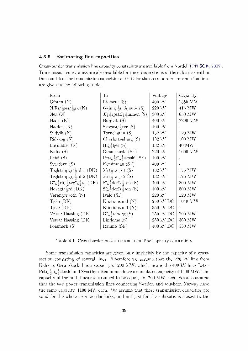
4.3.5 Estimating line capacities

Cross-border transmission line capacity constraints are available from Nordel [ENTSOE, 2007].

Transmission constraints are also available for the cross-sections of the sub areas within

the countries The transmission capacities at 0 C for the cross-border transmission lines

are given in the following table.

From To Voltage Capacity

Ofoten (N) Rietsem (S) 400 kV 1350 MW

N.Rï¾12ssï¾

12ga (N) Gejmï¾1

2n-Ajaure (S) 220 kV 415 MW

Nea (N) Jï¾12rpstrï¾

12mmen (S) 300 kV 650 MW

Hasle (N) Borgvik (S) 400 kV 2200 MW

Halden (N) Skogssï¾12ter (S) 400 kV -

Sildvik (N) Tornehamn (S) 132 kV 120 MW

Eidskog (N) Charlottenberg (S) 132 kV 100 MW

Lutufallet (N) Hï¾12 ljes (S) 132 kV 40 MW

Kalix (S) Ossauskoski (SF) 220 kV 1600 MW

Letsi (S) Petï¾12 jï¾

12skoski (SF) 400 kV -

Svartbyn (S) Keminmaa (SF) 400 kV -

Teglstrupgï¾12rd 1 (DK) Mï¾1

2rarp 1 (S) 132 kV 175 MW

Teglstrupgï¾12rd 2 (DK) Mï¾1

2rarp 2 (S) 132 kV 175 MW

Gï¾12rlï¾

12segï¾

12rd (DK) Sï¾1

2derï¾12sen (S) 400 kV 800 MW

Hovegï¾12rd (DK) Sï¾1

2derï¾12sen (S) 400 kV 800 MW

Varangerboth (N) Ivalo (SF) 220 kV 120 MW

Tjele (DK) Kristiansand (N) 250 kV DC 1040 MW

Tjele (DK) Kristiansand (N) 350 kV DC -

Vester Hassing (DK) Gï¾12teborg (S) 250 kV DC 290 MW

Vester Hassing (DK) Lindome (S) 280 kV DC 360 MW

Forsmark (S) Raumo (SF) 400 kV DC 550 MW

Table 4.1: Cross-border power transmission line capacity constraints

Some transmission capacities are given only implicitly by the capacity of a cross-

section consisting of several lines. Therefore we assume that the 220 kV line from

Kalix to Ossauskoski has a capacity of 200 MW, which means the 400 kV lines Letsi-

Petï¾12 jï¾

12skoski and Svartbyn-Keminmaa have a cumulated capacity of 1400 MW. The

capacity of the both lines are assumed to be equal, i.e. 700 MW each. We also assume

that the two power transmission lines connecting Sweden and southern Norway have

the same capacity, 1100 MW each. We assume that these transmission capacities are

valid for the whole cross-border links, and not just for the substations closest to the

39

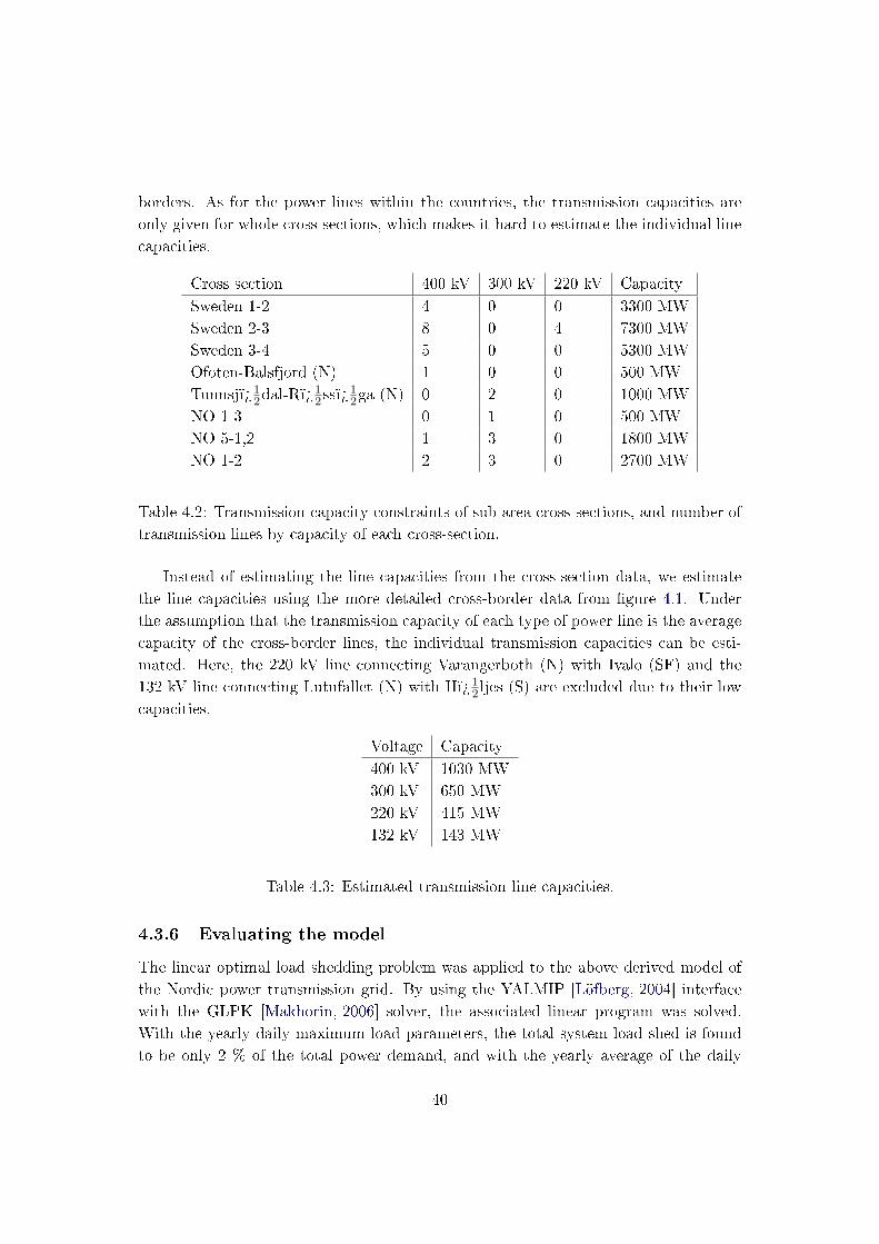
borders. As for the power lines within the countries, the transmission capacities are

only given for whole cross-sections, which makes it hard to estimate the individual line

capacities.

Cross section 400 kV 300 kV 220 kV Capacity

Sweden 1-2 4 0 0 3300 MW

Sweden 2-3 8 0 4 7300 MW

Sweden 3-4 5 0 0 5300 MW

Ofoten-Balsfjord (N) 1 0 0 500 MW

Tunnsjï¾12dal-Rï¾

12ssï¾

12ga (N) 0 2 0 1000 MW

NO 1-3 0 1 0 500 MW

NO 5-1,2 1 3 0 1800 MW

NO 1-2 2 3 0 2700 MW

Table 4.2: Transmission capacity constraints of sub area cross-sections, and number of

transmission lines by capacity of each cross-section.

Instead of estimating the line capacities from the cross-section data, we estimate

the line capacities using the more detailed cross-border data from gure 4.1. Under

the assumption that the transmission capacity of each type of power line is the average

capacity of the cross-border lines, the individual transmission capacities can be esti-

mated. Here, the 220 kV line connecting Varangerboth (N) with Ivalo (SF) and the

132 kV line connecting Lutufallet (N) with Hï¾12 ljes (S) are excluded due to their low

capacities.

Voltage Capacity

400 kV 1030 MW

300 kV 650 MW

220 kV 415 MW

132 kV 143 MW

Table 4.3: Estimated transmission line capacities.

4.3.6 Evaluating the model

The linear optimal load shedding problem was applied to the above derived model of

the Nordic power transmission grid. By using the YALMIP [Löfberg, 2004] interface

with the GLPK [Makhorin, 2006] solver, the associated linear program was solved.

With the yearly daily maximum load parameters, the total system load shed is found

to be only 2 % of the total power demand, and with the yearly average of the daily

40

maximum loads, the total system load shed was found to be 0 %. This shows that the

accuracy of our approximations is very high and the model is usable in practice.

A reasonable question to ask, is whether the model of the Nordic power transmission

grid is in accordance with rules regulating the common electricity market. For instance,

does it satisfy the N −1 criterion? For the evaluation of the N −1 criterion, we use the

yearly average of the daily maximum loads. For each N − 1 contingency, that is the

disconnection of any single power line, the optimal load shedding problem was solved,

and the load shed was calculated. There are 51 power line contingencies that result in

system load shed, but none which result in a total load shed of more than 1.6 %. Many

of these contingencies are dead-end lines, who's removal necessarily result in system

load shed. Also, since no single line contingency causes considerable damage to the

system, other than local, the N − 1 criterion is considered to be essentially fullled.

4.4 Simulations of correlated system failures in the Nordic

power grid

In this section we examine the eects of correlated system faults on the statistics of

the minimum total system load shed. The study of correlated faults in power systems

is motivated by the increased deployment of of-the-shelf hardware and software in

SCADA systems governing the power systems. When identical software is deployed in

several system components, software faults between those components are likely to be

correlated. Hence we will examine the eects of increasing correlations on the statistics

of the load shed distribution, and in particular on the mean and the variance of the

system load shed. In the following section we will consider failures of the form of power

line disconnections. We model the disconnection of power line i as a binary random

variable Xi ∈ 0, 1 where Xi = 0 translates to line i being fully functional with all

parameters set to default, and Xi = 1 translates to line i being disconnected, i.e. the

admittance of line i being 0. Hence, we consider the Bernoulli distribution

P (X1 = Y1, . . . , Xnp = Ynp) ∀ Yi ∈ 0, 1

Since parameterizing the full Bernoulli distribution would require nnp ≈ 10216 variables,

we will only consider the rst two central moments of the joint bernoulli distribution,

i.e.

Xi = E[Xi] ∀i ∈ 1, . . . , npσij = E

[(Xi − Xi)(Xj − Xj)

]∀ (i, j) ∈ 1, . . . , np2

which requires only n2p + np = 519120 variables. To consider the consequences of

increasing correlations Xi = 0.02 is kept constant, while σij is increased.

41

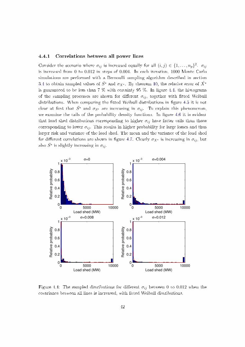
4.4.1 Correlations between all power lines

Consider the scenario where σij is increased equally for all (i, j) ∈ 1, . . . , np2. σijis increased from 0 to 0.012 in steps of 0.004. In each iteration, 1000 Monte Carlo

simulations are performed with a Bernoulli sampling algorithm described in section

3.4 to obtain sampled values of S∗ and σX∗ . By theorem 10, the relative error of X∗

is guaranteed to be less than 7 % with certainty 95 %. In gure 4.4, the histograms

of the sampling processes are shown for dierent σij , together with tted Weibull

distributions. When comparing the tted Weibull distributions in gure 4.5 it is not

clear at rst that S∗ and σS∗ are increasing in σij . To explain this phenomenon,

we examine the tails of the probability density functions. In gure 4.6 it is evident

that load shed distributions corresponding to higher σij have fatter tails than those

corresponding to lower σij . This results in higher probability for large losses and thus

larger risk and variance of the load shed. The mean and the variance of the load shed

for dierent correlations are shown in gure 4.7. Clearly σX∗ is increasing in σij , but

also S∗ is slightly increasing in σij .

0 5000 100000

0.2

0.4

0.6

0.8

1x 10

−3 σ=0

Load shed (MW)

Rela

tive p

robabili

ty

0 5000 100000

0.2

0.4

0.6

0.8

1x 10

−3 σ=0.004

Load shed (MW)

Rela

tive p

robabili

ty

0 5000 100000

0.2

0.4

0.6

0.8

1x 10

−3 σ=0.008

Load shed (MW)

Rela

tive p

robabili

ty

0 5000 100000

0.2

0.4

0.6

0.8

1x 10

−3 σ=0.012

Load shed (MW)

Rela

tive p

robabili

ty

Figure 4.4: The sampled distributions for dierent σij between 0 to 0.012 when the

covariance between all lines is increased, with tted Weibull distributions.

42

0 500 1000 1500 2000 2500 30000

0.1

0.2

0.3

0.4

0.5

0.6

0.7

0.8

0.9

1x 10

−3

Load shed (MW)

Pro

babili

ty

σ=0

σ=0.004

σ=0.008

σ=0.012

Figure 4.5: Fitted Weibull distributions of the Monte Carlo sampled load shed distri-

bution for σij from 0 to 0.012, when the covariance between all lines is increased.

43

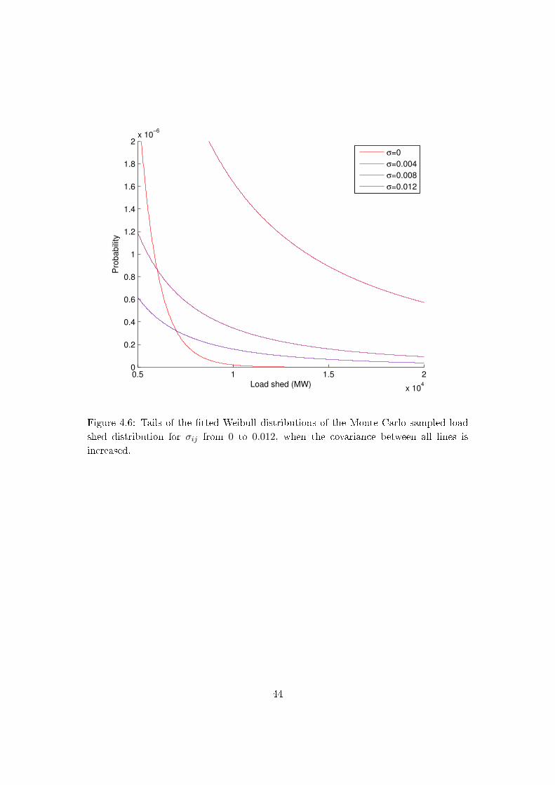
0.5 1 1.5 2

x 104

0

0.2

0.4

0.6

0.8

1

1.2

1.4

1.6

1.8

2x 10

−6

Load shed (MW)

Pro

babili

ty

σ=0

σ=0.004

σ=0.008

σ=0.012

Figure 4.6: Tails of the tted Weibull distributions of the Monte Carlo sampled load

shed distribution for σij from 0 to 0.012, when the covariance between all lines is

increased.

44

0 0.002 0.004 0.006 0.008 0.01 0.012 0.014 0.016500

1000

1500

2000

2500

3000

3500

4000

4500

σij

X∗ ,σX

∗

X*

σX

*

Figure 4.7: Expected value and standard deviation (MW) of the total load shed for for

σij from 0 to 0.012.

4.4.2 Correlations between incident power lines

For large power systems such as the Nordic grid, failures of remote power lines may

only have marginal eects on distant load nodes in terms of load shed. Therefore we

here consider the scenario where only the failures of incident power lines are correlated.

Let σij be increased from 0 to 0.016 in steps of 0.004 if and only if the power lines

i and j are connected to the same bus, otherwise σij = 0. Xi = 0.02 is again kept

constant. In gure 4.8, the histograms of the sampling processes are shown for dierent

σij , together with tted Weibull distributions. The mean and the variance of the load

shed for dierent correlations are shown in gure 4.11. Clearly both S∗ and σX∗ are

strongly increasing in σij , and the eect of increasing correlations is much higher than

when all power line failures are correlated.

45

0 5000 100000

0.2

0.4

0.6

0.8

1x 10

−3 σ=0

Load shed (MW)

Re

lative

pro

ba

bili

ty

0 5000 100000

0.2

0.4

0.6

0.8

1x 10

−3 σ=0.004

Load shed (MW)

Re

lative

pro

ba

bili

ty

0 5000 100000

0.2

0.4

0.6

0.8

1x 10

−3 σ=0.008

Load shed (MW)

Re

lative

pro

ba

bili

ty

0 5000 100000

0.2

0.4

0.6

0.8

1x 10

−3 σ=0.012

Load shed (MW)

Re

lative

pro

ba

bili

ty

0 5000 100000

0.2

0.4

0.6

0.8

1x 10

−3 σ=0.016

Load shed (MW)

Re

lative

pro

ba

bili

ty

Figure 4.8: The sampled distributions for dierent σij between 0 to 0.016 when the

covariance between neighboring lines is increased, with tted Weibull distributions.

46

0 500 1000 1500 2000 2500 30000

0.1

0.2

0.3

0.4

0.5

0.6

0.7

0.8

0.9

1x 10

−3

Load shed (MW)

Pro

babili

ty

σ=0

σ=0.004

σ=0.008

σ=0.012

σ=0.016

Figure 4.9: Fitted Weibull distributions of the Monte Carlo sampled load shed dis-

tribution for σij from 0 to 0.016, when the covariance between neighboring lines is

increased.

47

0.5 1 1.5 2

x 104

0

0.2

0.4

0.6

0.8

1

1.2

1.4

1.6

1.8

2x 10

−6

Load shed (MW)

Pro

babili

ty

σ=0

σ=0.004

σ=0.008

σ=0.012

σ=0.016

Figure 4.10: Tails of the tted Weibull distributions of the Monte Carlo sampled load

shed distribution for σij from 0 to 0.016, when the covariance between neighboring

lines is increased.

48

0 0.002 0.004 0.006 0.008 0.01 0.012 0.014 0.016500

600

700

800

900

1000

1100

1200

1300

1400

σij

X∗ ,σX

∗

X*

σX

*

Figure 4.11: Expected value and standard deviation (MW) of the total load shed for

σij from 0 to 0.012.

4.4.3 Correlations between power lines incident to PMUs

We here consider the scenario where failures are correlated only amongst lines incident

to nodes with phasor measurement units (PMUs). This scenario is motivated by the use

of identical software and hardware in PMUs, which could cause correlations between

failures of these nodes, and hence the incident lines. In gure 4.12, the histograms

of the sampling processes are shown for dierent σij , together with tted Weibull

distributions. When comparing the tted Weibull distributions in gure 4.13 it is clear

that S∗ and σS∗ are increasing in σij . The mean and the variance of the load shed for

dierent correlations are shown in gure 4.14. While σX∗ is not increasing in σij , S∗

is increasing by a factor 15 with increasing σij .

49

0 5000 100000

0.2

0.4

0.6

0.8

1x 10

−3 σ=0

Load shed (MW)

Rela

tive p

robabili

ty

0 5000 100000

0.2

0.4

0.6

0.8

1x 10

−3 σ=0.004

Load shed (MW)

Rela

tive p

robabili

ty

0 5000 100000

0.2

0.4

0.6

0.8

1x 10

−3 σ=0.008

Load shed (MW)

Rela

tive p

robabili

ty

0 5000 100000

0.2

0.4

0.6

0.8

1x 10

−3 σ=0.012

Load shed (MW)

Rela

tive p

robabili

ty

0 5000 100000

0.2

0.4

0.6

0.8

1x 10

−3 σ=0.016

Load shed (MW)

Rela

tive p

robabili

ty

Figure 4.12: The sampled distributions for dierent σij between 0 to 0.016 when the

covariance between power lines incident to PMU nodes is increased, with tted Weibull

distributions.

50

0 500 1000 1500 2000 2500 30000

0.1

0.2

0.3

0.4

0.5

0.6

0.7

0.8

0.9

1x 10

−3

Load shed (MW)

Pro

babili

ty

σ=0

σ=0.004

σ=0.008

σ=0.012

σ=0.016

Figure 4.13: Fitted Weibull distributions of the Monte Carlo sampled load shed dis-

tribution for σij from 0 to 0.016, when the covariance between power lines incident to

PMU nodes is increased.

51

0 0.002 0.004 0.006 0.008 0.01 0.012 0.014 0.0160

1000

2000

3000

4000

5000

6000

7000

8000

σij

X∗ ,σX

∗

X*

σX

*

Figure 4.14: Expected value and standard deviation (MW) of the total load shed for

σij from 0 to 0.016, when correlations are increased for power lines incident to PMU

nodes.

4.5 Applications

4.5.1 Interactions between TSOs

In this section we will give an introduction to some possible game theoretic applications

of the Monte Carlo methods introduced in section 3.3. For a review of game theory, the

interested reader is referred to Appendix C.5 and references therein. As we have seen

in sections 4.4.1 - 4.4.3, increasing correlations will typically cause both the expected

value and the variance of the system load shed to increase. In this model, we assume

that the TSOs can control the correlations between power line failures, whereas the the

means are kept constant. Consider the model of the Nordic power grid from section

4.3, with statistics on the power line failures. Let E[Xi] = 0.02 ∀i. Let the strategy of

each TSO be denoted si, and the set of all strategies S = s1, s2, s3, s4. Assume that

all TSOs, i.e. Denmark, Norway, Sweden and Finland, have two available strategies, s1

52

and s2, which will be aecting all nodes within their subsystem directly. We say that a

node is aected by either strategy 1 or 2. Let the covariance matrix of the power line

failures be given by σ =[σij], where:

σij =

σ if vi or vj is incident to a PMU and not

both nodes are aected by strategy 2

0 otherwise

(4.3)

Furthermore, we assume that there is a direct cost associated with strategy 2, which is

cpmu per PMU node, whereas there is no direct cost associated with strategy 1.

Note 1. Strategy 1 can be interpreted as a passive strategy where the TSO takes no

actions to decrease correlations between power lines, whereas strategy 2 can be seen as

an active strategy where the TSO reduces failure correlations but has to pay the costs

for this.

Note 2. For the correlation between two lines controlled by two dierent TSOs to be

0, both TSOs have to use strategy 2.

By using the Monte Carlo sampling framework of section 3.3, we can get approx-

imative costs associated with the TSOs strategies. The total number of strategies is

24 = 16, for which each strategy corresponds to a dierent covariance matrix σ. Let

the payo function for each TSO i be given by:

fi(S) = S∗i (C(S), d) + α · σi,S∗(C(S), d) + δ(si − 2) · cpmu · npmui (4.4)

where δ(0) = 1, δ(x) = 0 ∀x 6= 0 and npmui is the number of PMUs belonging to TSO

i. S∗i (C(S), d) and σi,S∗(C(S), d) are the mean and variance of the load shed in the

subsystem of TSO i. We assume that TSOs do not cooperate when choosing strategies,

and that the objective of the TSOs is to minimize their own total costs. The resulting

game is a non-cooperative game with nite strategy space, hence there exists a mixed

strategy Nash equilibrium for the game. We use an algorithm for computing the Nash

equilibrium described in [Chatterjee, 2009]. Also, we dene the social optimal strategy

as:

Ss = argmin

S∗(C(S), d) + α · σS∗(C(S), d) +

4∑i=1

δ(si − 2) · cpmu · npmui

(4.5)

Note that here the expected value and the variance are taken over the whole power

grid. By studying how the Nash equilibrium strategy and the social optimal strategy

vary with cpmu, we solve the above problems for cpmu ∈ [0, 200] in steps of 0.01, and

x α = 2. In gure 4.15 the total operational cost is shown for dierent cpmu under

53

0 20 40 60 80 100 120 140 160 180 2002000

2500

3000

3500

Investment cost per PMU, cpmu

Tota

l opera

tional cost

Nash equilibrium cost

Social optimal cost

Figure 4.15: The social cost is shown under increasing values of cpmu, under both the

socially optimal strategy and the Nash equilibrium strategy.

cpmu DK NO SE FI

[0, 11.0] 2 1 2 1

[11.0, 68.8] 1 1 2 1

[68.8,∞] 1 1 1 1

Table 4.4: Nash equilibrium strategies for dierent values of cpmu

both the social optimal strategy and the Nash equilibrium strategy. Of course, the

socially optimal cost is less than or equal than the cost under the Nash equilibrium

strategy. The gap between the two costs, i.e. the cost of anarchy, is relatively high

as seen in gure 4.15. The Nash equilibrium strategies of the TSOs as a function of

cpmu are shown in table 4.4. We note that all equilibrium strategies are pure strategies.

The socially optimal strategy is shown in table 4.5. There are many other possible

interactions between TSOs that could be modeled using a game theoretic framework.

54

cpmu DK NO SE FI

[0, 184.1] 1 2 2 1

[184.1,∞] 1 1 1 1

Table 4.5: Socially optimal strategies for dierent values of cpmu

This small example highlights that the interdependence between TSOs introduced by

the correlations between system failures, can be analyzed in a game theoretic setting.

Also, the gap between the costs highlights the need of cooperative network design.

4.6 Discussion

Simulations indicate that the increased correlations between power line failures can

cause either the expected value or the variance of the load shed to increase, or cause

both to increase simultaneously. The aect of correlated failures is highly dependent

on the structure of the correlations, as seen in the previous simulations. We have

studied three dierent correlation structures of failures, where either all power lines

are correlated, only incident lines are correlated or where power lines incident to PMU

nodes are correlated. All these scenarios produce dierent load shed distributions with

all dierent statistical properties. Simulations show that increased correlations can

increase the expected load shed in the Nordic grid by as much as a factor 15.

Although simulations indicate that correlations increase the expected value of the

system load shed, it is easy to nd counterexamples where increased correlations be-

tween power line failures decrease the expected load shed. The simplest possible coun-

terexample is shown below.

Example 4.6.1. Consider a 3-bus and 2-line power network shown in gure 4.16.

Let the demand bus have demand −d, and the generation bus a capacity g ≥ d, and

the line parameters be such that the demand is satised under normal operation. It

can be shown that the expected load shed of the system is 1 − σ12, where σ12 is the

covariance between the failures of power lines l1 and l2. The intuition behind this

counterexample is that while the probability of both lines failing increases, the probability

of each failing individually decreases, with the result that the total probability of any line

failing decreases.

55

g n dl1 l2

Figure 4.16: Topology of a 3-bus, 2-line power network where increased correlations

between power line failures result in decreased system load shed. g is a generation bus,

d a demand bus and n a demand with power demand 0.

We here state sucient conditions under which increased correlations of power line

failures imply increased expected load shed.

Proposition 2. Let the power system satisfy the n−k criterion, i.e. the disconnection

of any k power lines does not induce any necessary load shedding. Furthermore, assume

that all contingencies with at least k+ 1 line failures induce a total system load shed c.

Assume, wlog, that the moment φ1,...,k+1 = E[X1 · . . . ·Xk+1] increases by ∆φ, but all

other moments E[Xi1 · . . . ·Xil ] are constant. Then

1. The central moment σ1,...,k+1 = E[(X1 − X1) · . . . · (Xk+1 − Xk+1)

]also increases

by ∆φ.

2. All other central moments of order less than or equal to k + 1 remain constant.

3. The expected load shed S∗ increases by c ·∆φ.

4. If E[Xi] < 1/2∀φ, the variance of the load shed, σS∗, increases by c2 ·∆φ, where0 < c ≤ c.

A proof is given in Appendix . The following corollary follows directly from propo-

sition 2.

Corollary 12. Assume that all conditions of proposition 2 still hold, except that all

contingencies with at least k + 1 line failures induce a system load shed of at least c.

In this case the results of proposition 2 hold instead for the lower bound S∗ ≤ S∗ of thesystem load shed, which is the total system load shed assuming all line failures result in

the same system load shed c.

We note that the power network in example 4.6.1 fails to satisfy the criteria of

proposition 2. In particular, it fails to satisfy the N − 1 criterion, because the second

order central moment is increased.

56

Chapter 5

Conclusions and future research

In this work we have shown that increased correlations between failures can dramati-

cally increase the expected costs in terms of system load shed, although the expected

values of the failure probabilities are kept constant. Furthermore we have shown that

increased correlations can also increase the variance of the system load shed, thus

increasing the probability of large system load sheds. We have shown our results theo-

retically under special conditions, and provided empirical results for a large-scale model

of the Nordic power system.

Power systems are very complex systems, and estimating failure distributions a pri-

ory based on the statistics of the power system is in general not possible without using

Monte Carlo based methods. Furthermore, deterministic reliability criteria such as the

N − 1 criterion are not well-suited for correlated and more complex failure statistics.

Therefore we believe that Monte Carlo based methods for determining reliability of

power systems will play an important part in the future, and the methods will con-

tinue to evolve. In many situations, cascading failures further aggravate the state of a

partially failing power system, leading to even larger losses. In future work, it would

be interesting to consider the impact of correlated failures while also considering cas-

cading failures. It would also be interesting to acquire real data from TSOs and apply

our framework to this data. Also, it would be of interest to study if the conditions

under which the expected value and the variance of the load shed are increasing in the

correlations, can be relaxed and made practically useful.

57

Bibliography

[Abur and Exposito, 2004] Abur, A. and Exposito, A. G. (2004). Power System State

Estimation: Theory and Implementation; electronic version. Dekker, Abingdon.

[Albadi and El-Saadany, 2007] Albadi, M. and El-Saadany, E. (2007). Demand re-

sponse in electricity markets: An overview. In Power Engineering Society General

Meeting, 2007. IEEE, pages 1 5.

[Allan and Billinton, 2000] Allan, R. and Billinton, R. (2000). Probabilistic assessment

of power systems. Proceedings of the IEEE, 88(2):140 162.

[Amanullah et al., 2005] Amanullah, M., Kalam, A., and Zayegh, A. (2005). Network

security vulnerabilities in scada and ems. In Transmission and Distribution Confer-

ence and Exhibition: Asia and Pacic, 2005 IEEE/PES, pages 1 6.

[Amin, 2002] Amin, M. (2002). Security challenges for the electricity infrastructure.

Computer, 35(4):8 10.

[Anghel et al., 2007] Anghel, M., Werley, K. A., and Motter, A. E. (2007). Stochastic

model for power grid dynamics. In System Sciences, 2007. HICSS 2007. 40th Annual

Hawaii International Conference on, pages 113 113.

[Arroyo and Galiana, 2005] Arroyo, J. and Galiana, F. (2005). On the solution of the

bilevel programming formulation of the terrorist threat problem. Power Systems,

IEEE Transactions on, 20(2):789 797.

[Bar-Shalom et al., 2002] Bar-Shalom, Y., Kirubarajan, T., and Li, X.-R. (2002). Es-

timation with Applications to Tracking and Navigation. John Wiley & Sons, Inc.,

New York, NY, USA.

[Bereanu, 1976] Bereanu, B. (1976). The continuity of the optimum in parametric

programming and applications to stochastic programming. Journal of Optimization

Theory and Applications, 18:319333. 10.1007/BF00933815.

58

[Bertsch et al., 2005] Bertsch, J., Carnal, C., Karlson, D., McDaniel, J., and Vu, K.

(2005). Wide-area protection and power system utilization. Proceedings of the IEEE,

93(5):997 1003.

[Billinton and Allan, 1995] Billinton, R. and Allan, R. N. (1995). Reliability evaluation

of power systems.

[Billinton and Khan, 1992] Billinton, R. and Khan, E. (1992). A security based ap-

proach to composite power system reliability evaluation. Power Systems, IEEE

Transactions on, 7(1):65 72.

[Billinton and Wang, 1999] Billinton, R. and Wang, P. (1999). Teaching distribution

system reliability evaluation using monte carlo simulation. Power Systems, IEEE

Transactions on, 14(2):397 403.

[Boyd and Vandenberghe, 2004] Boyd, S. and Vandenberghe, L. (2004). Convex Opti-

mization. Cambridge University Press.

[Brugg, 2006] Brugg (2006). High voltage xlpe cable systems, technical user guide.

[Brunekreeft et al., 2005] Brunekreeft, G., Neuho, K., and Newbery, D. (2005). Elec-

tricity transmission: An overview of the current debate. Utilities Policy, 13(2):73

93. Electricity Transmission.

[Chatterjee, 2009] Chatterjee, B. (2009). An optimization formulation to compute nash

equilibrium in nite games. In Methods and Models in Computer Science, 2009.

ICM2CS 2009. Proceeding of International Conference on, pages 1 5.

[Chertkov et al., 2010] Chertkov, M., Pan, F., and Stepanov, M. G. (2010). Predicting

failures in power grids. Technical Report arXiv:1006.0671. LA-UR 10-02934.

[Consulting, 2002] Consulting (2002). Economic assessment of rto policy.

[da Silva et al., 2004] da Silva, A., de Resende, L., da Fonseca Manso, L., and Billinton,

R. (2004). Well-being analysis for composite generation and transmission systems.

Power Systems, IEEE Transactions on, 19(4):1763 1770.

[Daneels and Salter, 1999] Daneels, A. and Salter, W. (1999). What is scada? Interna-

tional Conference on Accelerator and Large Experimental Physics Control Systems,

Trieste, Italy.

[Daniel Karlsson and Johannesson, 2008] Daniel Karlsson, S. L. and Johannesson, T.

(2008). Phasor measurements recording south sweden ? eastern denmark.

59

[Diestel, 2005] Diestel, R. (2005). Graph Theory, volume 173 of Graduate Texts in

Mathematics. Springer-Verlag, Heidelberg, third edition.

[Due and Pan, 1997] Due, D. and Pan, J. (1997). An overview of value at risk. The

Journal of Derivatives, 4(3):7 49.

[ENTSOE, 2007] ENTSOE (2007). Nordic grid code.

[Fernandez and Fernandez, 2005] Fernandez, J. D. and Fernandez, A. E. (2005). Scada

systems: vulnerabilities and remediation. J. Comput. Small Coll., 20:160168.

[Fisher et al., 2008] Fisher, E., O'Neill, R., and Ferris, M. (2008). Optimal transmis-

sion switching. Power Systems, IEEE Transactions on, 23(3):1346 1355.

[Flatabo et al., 2003] Flatabo, N., Doorman, G., Grande, O., Randen, H., and Wan-

gensteen, I. (2003). Experience with the nord pool design and implementation. Power

Systems, IEEE Transactions on, 18(2):541 547.

[Fredriksson and Johansson, 2010] Fredriksson, Y. and Johansson, M. (2010). Ei ser

positivt på förslaget att sverige delas in i fyra elprisområden'. Energimarknadsin-

spektionen.

[Gotham and Heydt, 1998] Gotham, D. and Heydt, G. (1998). Power ow control and

power ow studies for systems with facts devices. Power Systems, IEEE Transactions

on, 13(1):60 65.

[Hingorani, 1993] Hingorani, N. (1993). Flexible ac transmission. Spectrum, IEEE,

30(4):40 45.

[Hogan, 1998] Hogan, W. (1998). Independent system operator (iso) for a competitive

electricity market.

[Huneault and Galiana, 1991] Huneault, M. and Galiana, F. (1991). A survey of the

optimal power ow literature. Power Systems, IEEE Transactions on, 6(2):762770.

[Joskow, 2005] Joskow, P. L. (2005). Transmission policy in the united states. Utilities

Policy, 13(2):95 115. Electricity Transmission.

[Karlsson et al., 2004] Karlsson, D., Hemmingsson, M., and Lindahl, S. (2004). Wide

area system monitoring and control - terminology, phenomena, and solution imple-

mentation strategies. Power and Energy Magazine, IEEE, 2(5):68 76.

[Kinney et al., 2005] Kinney, R., Crucitti, P., Albert, R., and Latora, V. (2005). Model-

ing cascading failures in the north american power grid. The European Physical Jour-

nal B - Condensed Matter and Complex Systems, 46:101107. 10.1140/epjb/e2005-

00237-9.

60

[Leirbukt et al., 2008] Leirbukt, A., Breidablik, O., Gjerde, J., Korba, P., Uhlen, K.,

and Vormedal, L. (2008). Deployment of a scada integrated wide area monitoring sys-

tem. In Transmission and Distribution Conference and Exposition: Latin America,

2008 IEEE/PES, pages 1 6.

[Lu and Abur, 2002] Lu, Y. and Abur, A. (2002). Static security enhancement via

optimal utilization of thyristor-controlled series capacitors. Power Systems, IEEE

Transactions on, 17(2):324 329.

[Löfberg, 2004] Löfberg, J. (2004). Yalmip : A toolbox for modeling and optimization

in MATLAB. In Proceedings of the CACSD Conference, Taipei, Taiwan.

[Macke et al., 2009] Macke, J. H., Berens, P., Ecker, A. S., Tolias, A. S., and Bethge,

M. (2009). Generating spike trains with specied correlation coecients. Neural

Computation, 21(2):397423. PMID: 19196233.

[Makhorin, 2006] Makhorin, A. (2006). GNU Linear Programming Kit, Version 4.9.

GNU Software Foundation, http://www.gnu.org/software/glpk/glpk.html.

[Massoud and Wollenberg, 2005] Massoud and Wollenberg, B. F. (2005). Toward a

smart grid: power delivery for the 21st century. IEEE Power and Energy Magazine,

3(5):3441.

[MATLAB, 2010] MATLAB (2010). version 7.11.0 (R2010b). The MathWorks Inc.,

Natick, Massachusetts.

[McNe, 2002] McNe, J. (2002). The global positioning system. Microwave Theory

and Techniques, IEEE Transactions on, 50(3):645 652.

[Murphy and Wu, 1993] Murphy, L. and Wu, F. (1993). An open design approach for

distributed energy management systems. Power Systems, IEEE Transactions on,

8(3):1172 1179.

[Nash, 1951] Nash, J. (1951). Non-cooperative games. The Annals of Mathematics,

54(2):pp. 286295.

[Nordel, 2006] Nordel (2006). Agreement (translation) regarding operation of the in-

terconnected nordic power system (system operation agreement).

[Nordpool, 2009] Nordpool (2009). Anual report.

[Phadke, 1993] Phadke, A. (1993). Synchronized phasor measurements in power sys-

tems. Computer Applications in Power, IEEE, 6(2):10 15.

61

[Phadke, 2002] Phadke, A. (2002). Synchronized phasor measurements-a historical

overview. In Transmission and Distribution Conference and Exhibition 2002: Asia

Pacic. IEEE/PES, volume 1, pages 476 479 vol.1.

[Pinar et al., 2010] Pinar, A., Meza, J., Donde, V., and Lesieutre, B. (2010). Opti-

mization strategies for the vulnerability analysis of the electric power grid. SIAM

Journal on Optimization, 20(4):17861810.

[Pollitt, 2008] Pollitt, M. (2008). The arguments for and against ownership unbundling

of energy transmission networks. Energy Policy, 36(2):704 713.

[Preedavichit and Srivastava, 1998] Preedavichit, P. and Srivastava, S. C. (1998). Op-

timal reactive power dispatch considering facts devices. Electric Power Systems

Research, 46(3):251 257.

[Roy Billinton, 1994] Roy Billinton, Billinton, W. L. (1994). Reliability assessment of

electrical power systems using monte carlo methods.

[Saarinen, 2010] Saarinen, K. (2010). Application of phasor measurement units and

wide-area measurement systems in nland.

[Salmeron et al., 2004] Salmeron, J., Wood, K., and Baldick, R. (2004). Analysis of

electric grid security under terrorist threat. Power Systems, IEEE Transactions on,

19(2):905 912.

[SvK, 2009] SvK (2009). Fou-plan 2009 - 2011'.

[Uhlen et al., 2008] Uhlen, K., Warland, L., Gjerde, J., Breidablik, O., Uusitalo, M.,

Leirbukt, A., and Korba, P. (2008). Monitoring amplitude, frequency and damping

of power system oscillations with pmu measurements. In Power and Energy Society

General Meeting - Conversion and Delivery of Electrical Energy in the 21st Century,

2008 IEEE, pages 1 7.

[Xiao et al., 2002] Xiao, Y., Song, Y., and Sun, Y. (2002). Power ow control approach

to power systems with embedded facts devices. Power Systems, IEEE Transactions

on, 17(4):943 950.

[Xu et al., 2008] Xu, Z., Ostergaard, J., Togeby, M., and Isleifsson, F. (2008). Eval-

uating frequency quality of nordic system using pmu data. In Power and Energy

Society General Meeting - Conversion and Delivery of Electrical Energy in the 21st

Century, 2008 IEEE, pages 1 5.

[Zhou and Bialek, 2005] Zhou, Q. and Bialek, J. (2005). Approximate model of euro-

pean interconnected system as a benchmark system to study eects of cross-border

trades. Power Systems, IEEE Transactions on, 20(2):782 788.

62

Appendix A

Notation

A.1 Mathematical notation

N 1, 2, . . .. The set of positive integersN0 0, 1, 2, . . .. The set of nonnegative integersZ . . . ,−1, 0, 1, . . .. The set of integers

, Componentwise inequality. For x, y ∈ Rn x y ⇔ xi ≤ yi ∀i = 1, . . . , n

xi The ith element of the column vector x

Aij The element on row i, column j of the matrix A

Ai· The ith row of the matrix A

A·j The jth column of the matrix A

[Aij ] The matrix with ijth element AijX The mean of the random variable X

σX The standard deviation of the random variable X

σ2X The variance deviation of the random variable X

dxe maxm ∈ Z|m ≤ x. The smallest integer greater than x

bxc minm ∈ Z|m ≥ x. The largest integer smaller than x

A.2 Denitions of terms

BDD Bad Data Detection is a lter which is able to detect corrupted measure-

ments [Abur and Exposito, 2004].

EMS Energy Management System is the technology used to monitor and con-

trol the power transmission in the electric power grid. EMS is used by

the system operators (SO), either TSOs or ISOs [Murphy and Wu, 1993,

Karlsson et al., 2004].

63

FACTS Flexible AC transmission system, is common name for technologies en-

abling ow control of AC currents in electric power transmission networks

[Hingorani, 1993, Gotham and Heydt, 1998, Xiao et al., 2002].

GPS Global Positioning System, is a satellite based high accuracy position-

ing and timing system owned and operated by the U.S. Department of

Defense [McNe, 2002].

ISO Independent System Operator, is an independent and non-prot organi-

zation responsible for the transmission planning for a regional power

transmission network. ISOs are typically ubiquitous in the USA,

where transmission operation and system ownership usually is separated

[Hogan, 1998, Pollitt, 2008, Joskow, 2005].

PDC Phasor Data Concentrator, is a mass storage for signal data from the

PMUs, accessible from the control center. from the control center

[Karlsson et al., 2004]

PMU Phasor Measurement Unit, sensor measuring current and voltage phasors

in real time. Having integrated GPS devices on board, PMUs are capa-

ble of producing synchronized and time-stamped phasor measurements

[Phadke, 1993, Phadke, 2002].

RTO Regional Transmission Organization, is an organization of ISOs with

the responsibility of power transmission planning over regions of several

ISOs. RTOs are most notably present in the USA [Consulting, 2002,

Joskow, 2005].

SCADA Supervisory Control And Data Acquisition, is the process of pulling data

from remote locations to permit operators to monitor and control re-

mote assets and processes in real time [Fernandez and Fernandez, 2005,

Daneels and Salter, 1999].

SO System Operator, See ISO.

TO Transmission Owner, is the owner of physical power transmission lines

[Joskow, 2005].

TSO Transmission System Operator. An entity which acts both as transmis-

sion owner (TO) and system operator (SO). A TSO owns the transmis-

sion lines, and is responsible for the electric power transmission, as well

as the physical maintenance of the power transmission system. This is

the typical structure of electric power transmission in European countries

[Brunekreeft et al., 2005, Pollitt, 2008].

WAMS Wide Area Measurement System, is the measurement system of PMUs

and PDC including the communication network [Karlsson et al., 2004,

Phadke, 2002].

64

Appendix B

Figures

Figure B.1: Operational states in the Nordic power system [ENTSOE, 2007]

65

HELSINKI

YllikkäläKoria

Loviisa

KymiNurmijärvi

Inkoo

Lieto

Rauma

Ulvila

Hyvinkää

Hikiä

Toivila

Olkiluoto

Petäjävesi

Alapitkä

Seinäjoki

Tuovila

Ventusneva

Huutokoski

Vuolijoki

Pikkarala

PirttikoskiPetäjäskoski

Keminmaa

Pyhänselkä

Alajärvi

Krivoporolsk

Alta

Utsjoki

Vajukoski

Ivalo

Vyborg

Stornorrfors

Sundsvall

KingiseppNarva

ESTONIATartu

LATVIARiga

Velikor

STOCKHOLM

LITHUANIA

Vilnius

Ignalina

Lida

Ross

Kaliningrad

Elk

Bialystok

KaunasZarnowiec

Gdansk

Zydowo

Ajaure

Letsi

Grundfors

Storfinnf.

Salten

JärpströmmenNea

Trondheim

Røssåga

TunnsjødalLinn-

vasselv

NORWAY

OSLO

Rjukan

Hasle Borgvik

Kristiansand

Bergen

Skogsäter

Göteborg

Nässjö

Norrköping

Oskarshamn

Karlshamn

Helsingborg

Ringhals

BarsebäckKruseberg

Ustka

Dunowo

Tjele

Kassø

KielAudorf

Flensburg

BrunsbüttelEmden

Lubmin

POLAND

KØBEN-HAVN

Pasewalk

Perleberg

BrokdorfRostockGüstrow

Hamb.IS

GERMANY

Bergum

HOLLAND

Enköping

(220)

(220)

DC

DC

DC

DC

DC

DC

DC

(220)

(110)

(220)

RDC

WestCoastcross-section

Narvik

Tromsø

TornehamnOfoten

(6)

(5)

(4)

(2)

(1)

(3)

A

(132)Kangasala

P1

FINLAND

RAC

SWEDEN

Cross-sectionno. 1

Cross-sectionno. 2

Cross-sectionno. 4

B

DENMARK

Stavanger

Figure B.2: Major transmission lines and area division in the Nordic grid

[ENTSOE, 2007]66

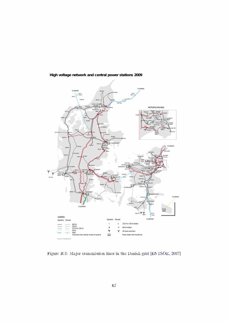
Highvoltagenetwork and central power stations 2009

TONORWAYTOSWEDEN

TOSWEDEN

TOSWEDEN

TOGERMANY

TOGERMANY

BredekærStarbakke

Konti-Skan

Nibstrup Dybvad

Hvorupgård

SkansenFredensdal

Skagerrak

250kV350kV

400kV

275kV285kV

400kV

400kV

Kontek

Frøstrup Klim

NORDJ YLLANDSVÆRKET

Ferslev

Nors

VilstedBedsted

Tinghøj

Hornbæk

Nr.Asmindrup

Valseværket

Borup

Teglstrupgård

Struer

Bilstrup

Loldrup

Tjele

Moselund

Mesballe

ÅstrupTrige

Hasle

HøskovMårslet

Malling

HørningVidebæk

HerningBjørnholt

Tange

StovstrupSdr. Felding

ThyregodAskær

Hatting

STUDSTRUPVÆRKET

MASNEDØVÆRKET

STIGSNÆSVÆRKET Blangslev

Haslev

Ringsted

StasevangAllerødgård

Mosedegård

J ersie

Bjæverskov

Ølstykke-gård

LyngerupSkibbygård Hovegård

Sperrestrupgård

Vindingegård

KamstrupKirkeskovgård

Idomlund

KnabberupKarlsgårde

RyttergårdLanderupgård

SKÆRBÆKVÆRKET

Estrupvej

1

Horns RevLykkegård

EndrupRevsing

Holsted

Ribe

ESBJ ERG-VÆRKET

Tyrstrup

Bredebro Kassø ENSTEDVÆRKET

Sønderborg

Graderup

Kingstrup

Abildskov

Svendborg

FYNSVÆRKET

Fraugde

Herslev

Østkraft

VestlollandRadsted

Rødby

Orehoved

Idestrup

Eskildstrup

Østerholm

Næstved

Rislev

Hejninge

KalundborgNovoSyd

Statoil Syd

Søstremose

ASNÆSVÆRKET

Nyrup

Torslunde

Karlstrup

OdenseSØ

Andst

Mosbæk

Mollerup

Ådalen

HåndværkervejÅlborgØst

Magstrup

Bramdrup

Fensmark

GlentegårdMåløvgård

Ejbygård

Flaskegård

Vejleå

Ishøj

METROPOLITANAREA

AVEDØRE-VÆRKET

Amager kbst

Kastrupkbst

Vigerslevkbst

Lindevang

Bellahøj

H.C.ØRSTEDVÆRKET

Brøndbygård

Ballerupgård

DyregårdGrønne-gård

AMAGER-VÆRKET

SVANEMØLLE-VÆRKET

Hovegård

Hareskovgård Bagsværd-

gård

VesterHassing

GørløsegårdKYNDBY-VÆRKET

Nysted

Storebælt

Operation Planned

Power stationwith transformer

132kVor 150kVstation

400kVstation

Off shorewind farm

2

Rødsand2

LEGENDS:

Operation Planned

400kV220kV132kVor 150kV60kVHVDCTransverse lines indicatenumber of systems

Herlufmagle

OstedgårdSpanager

Ramme

Kærbybro

Source: Energinet.dk

Figure B.3: Major transmission lines in the Danish grid [ENTSOE, 2007]

67

Appendix C

Mathematical preliminaries

C.1 Graphs

A simple graph is formally dened as a pairG = (V,E), such thatE ∈ [V ]2 [Diestel, 2005].

The elements of V are called vertices, and the elements of E are called edges.

Denition C.1. The number of vertices V and edges E are denoted |V | and |E|.

C.1.1 Undirected graphs

For a undirected graph, the edges can be represented as eij = (vi, vj) = (vj , vi) where vi, vj ∈V . An example of an undirected graph is shown in gure C.1, where the vertices are

enumerated from v1− v6, and the edges are enumerated from e1− e7.

v6

v1

v2

v3

v4

v5

e1

e2

e3

e4

e5

e6e7

Figure C.1: An example of an undirected graph.

68

C.1.2 Directed graphs

In a directed graph, often called a digraph, the edges are directed and have a starting

vertex and an end vertex. The edge of going from vertex vi to vj in a directed graph

can be represented as eij = (vi, vj). For directed graphs, the ordering of the vertices

matters, unlike in the case of an undirected graph. Digraphs are essential for modeling

power systems, as one has to be able to determine the direction of power ows. An

example of a digraph is shown in gure C.2, where the directions of the edges are

indicated with arrows.

v6

v1

v2

v3

v4

v5

e1

e2

e3

e4

e5

e6e7

Figure C.2: An example of a digraph.

C.1.3 Weighted graphs

The edges in a graph can be weighted by real numbers. The edges of a digraph are

associated with a real number which determines the weight of the edge. Formally eij =

(vi, vj , wij) = (vj , vi, wij) for undirected graphs, and eij = (vi, vj , wij) for digraphs.

Weighted graphs are essential for power system analysis, since the weights of the edges

can be used to represent dierent parameters of the power transmission lines. An

example of a weighted digraph is illustrated in gure C.3.

C.1.4 Vertex degree

Denition C.2. The degree (deg(·)) of a vertex is the number of edges incident to the

vertex.

Theorem 13. ∑v∈V

deg(v) = 2 |E|

69

v6

v1

v2

v3

v4

v5

w1

w2

w3

w4

w5

w6w7

Figure C.3: An example of a weighted digraph where the weights are: w1 = 1, w2 = 2,

w3 = 1, w4 = 2, w5 = 3, w6 = 1, w7 = 2.

Proof. The number of edges |E| can be determines by counting the edges incident to

each vertex, and summing. Since each edge is connected to exactly two vertices, each

edge will be counted exactly twice.

C.2 Matrix representations of graphs

Many interesting features of graphs can be studied by using matrix representations of

graphs. While there are many possible ways to represent graphs as matrices, we will

focus on two representations of importance to power system analysis.

C.2.1 Vertex-edge incidence matrix

Denition C.3. The vertex-edge incidence matrix for a directed matrix is formally

dened as:

A = [Aij ] where Aij =

1 if ei = (vj , u) ∈ E−1 if ei = (u, vj) ∈ E

0 otherwise

Example C.2.1. As an example, the vertex-edge incidence matrix for the digraph

70

shown in gure C.2 is:

A =

1 −1 0 0 0 0

0 1 −1 0 0 0

0 0 1 −1 0 0

−1 0 0 1 0 0

1 0 0 0 −1 0

0 −1 0 0 1 0

−1 0 0 0 0 1

Notice that Ae = 0, i.e. the rows sum to zero, because each edge leaves exactly one

vertex and arrives at exactly one vertex (corresponding to a −1 and 1 in the vertex-

edge incidence matrix respectively).

C.2.2 Laplacian

Denition C.4. The Laplacian of a graph is dened as:

L = [Lij ] where Lij =

deg(vi) if i = j

−1 if (vi, vj) ∈ E or (vj , vi) ∈ E0 otherwise

Example C.2.2. The Laplacian of the digraph shown in gure C.2 is:

L =

4 −1 0 −1 −1 −1

−1 3 −1 0 −1 0

0 −1 2 −1 0 0

−1 0 −1 2 0 0

−1 −1 0 0 2 0

−1 0 0 0 0 1

One may also dene the Laplacian for weighted graphs.

Denition C.5. The weighted Laplacian is dened as

Lw = [lij ] where lij =

∑

j wij for i where vj is adjacent to vi if i = j

−wij if (vi, vj) ∈ E−wji if (vj , vi) ∈ E

0 otherwise

where wij is the weight of the edge eij = (vi, vj).

By examining the structures of A and L, one nds that the Laplacian is closely

related to the vertex-edge incidence matrix. More precisely we have the following

theorem.

71

Theorem 14.

Lw = ATDwA (C.1)

where Dw = diag([wij ]).

Proof. For the diagonal elements of ATDwA it holds that

(ATDwA

)ii

=

|E|∑k=1

(AT )ikDwkkAki =

|E|∑k=1

AkiAkiDwkk =

|E|∑k=1

A2kiDwkk

where

Aki =

1 if ek = (vi, u) ∈ E−1 if ek = (u, vi) ∈ E

0 otherwise

Hence

|E|∑k=1

A2ki =

∑j

wij for i where vj is adjacent to vi = Lii

For the o-diagonal elements of ATDwA we have instead

(ATDwA

)ij

=

|E|∑k=1

ATikDwkkAkj =

|E|∑k=1

AkiAkjDwkk =

wij if ek = (vi, u) ∈ E ∧ ek = (vj , u) ∈ Ewji if ek = (u, vi) ∈ E ∧ ek = (u, vj) ∈ E−wij if ek = (vi, u) ∈ E ∧ ek = (u, vj) ∈ E−wji if ek = (u, vi) ∈ E ∧ ek = (vj , u) ∈ E

0 otherwise

=

−wij if (vi, vj) ∈ E−wji if (vj , vi) ∈ E

0 otherwise

= Lwij

Example C.2.3. For the weighted graph in gure C.3 the weight matrix is:

Dw =

1 0 0 0 0 0 0

0 2 0 0 0 0 0

0 0 2 0 0 0 0

0 0 0 2 0 0 0

0 0 0 0 3 0 0

0 0 0 0 0 1 0

0 0 0 0 0 0 2

72

and hence the weighted Laplacian is:

Lw =

8 −1 0 −2 −3 −2

−1 4 −2 0 −1 0

0 −2 4 −2 0 0

−2 0 −2 4 0 0

−3 −1 0 0 4 0

−2 0 0 0 0 2

Corollary 15.

L = ATA (C.2)

Proof. Follows from theorem 14 with Dw = I.

C.3 Probability theory

C.3.1 Random variables

To be able to dene the probability measure, we need to rely on the following denition.

Denition C.6. Let X be a set, and 2X be the power set of X. Σ ⊆ 2X is called a

σ-algebra if

• Σ 6= ∅

• A ∈ Σ⇒ X \A ∈ Σ

• Ai ∈ Σ, i = 1, 2, . . .⇒ ∪iAi ∈ Σ

Denition C.7. A probability space is a tuple (Ω,F , P ) where

• Ω is a non-empty set.

• F is a σ-algebra containing Ω.

• P : F → [0, 1]:

If Ai ⊆ F is a countable collection of pairwise disjoint sets, i.e. for

i 6= j Ai ∩Aj = ∅, then P (∪iAi) =∑

i P (Ai)

P (Ω) = 1

Ω is often referred to as the sample space, and is the set of all outcomes of a

probability experiment. F ⊆ 2Ω is the set of all events, where each event is a (possibly

empty) set of outcomes. The mapping P is often referred to as the probability measure.

P (A) is called the probability measure of the event A ⊆ F .

73

Example C.3.1. Consider a 6-sided unbiased die. The sample space is the set of all

outcomes, i.e.

Ω =1, 1, 1, 2, . . . , 6, 6

(C.3)

where e.g. 2 means the die shows a 2. Let the experiment be that the die is thrown

twice. Let us consider the event E that the sum of the two dice equals 10. This can be

translated into the events

E = 5, 5, 4, 6, 6, 4 (C.4)

The complete σ-algebra of the sample space is 2Ω, which contains 236 elements. Because

of the assumption of an unbiased die, and the natural assumption of independence of

the throws, the probability of each event is 16 ·

16 = 1

36 . Since the events are mutually

exclusive, the probability of the event E is

P (E) =1

36+

1

36+

1

36=

1

12(C.5)

C.3.2 Moments

Denition C.8. Let X ∈ Rn be a vector valued random variable, and µ(x) its asso-

ciated probability measure. The expected value X = E[X] of X, if existent, is dened

as

X = E[X] =

∫x dµ(x)

where∫·dµ(x) denotes the Lebesgue integral.

Note that the expected value may fail to exist in general, if the above integral

diverges.

Denition C.9. The m'th central moment of the random X with respect to the com-

ponents Xk1 , . . . , Xkm, where ki ∈ N ∀i ∈ 1, . . . ,m, is dened as

σk1,...,km = E

m∏i=1

(Xki − Xki

)Note that any central moment may fail to exist, if the according integral is divergent.

74

C.4 Linear programming

Denition C.10. A linear program (LP) is an optimization problem which can be

written in the form

maxx

cTx (C.6)

s.t. Ax b

where x, c ∈ Rn, b ∈ Rm, A ∈ Rm×n.

LPs are a special class of convex optimization problems, which is easily veried.

Denition C.11. A set X is convex i

∀x1, x2 ∈ X,∀λ ∈ [0, 1] : λx1 + (1− λ)x2 ∈ X

Denition C.12. A function f : Rn → R is convex i

• dom(f) is convex

• ∀x1, x2 ∈ dom(f), ∀λ ∈ [0, 1] : f(λx1 + (1− λ)x2) ≤ λf(x1) + (1− λ)f(x2)

Lemma 16. The LP in equation (C.6) is a convex optimization problem.

Proof. The objective function is convex since

cT (λx1 + (1− λ)x2) = λcTx1 + (1− λ)cTx2 ∀x1, x2

The feasible region F =x ∈ Rn|Ax ≤ b

is also convex since

x1, x2 ∈ F ⇒ λx1 + (1− λ)x2 ∈ F

since

A(λx1 + (1− λ)x2) = λAx1 + (1− λ)Ax2 ≤ λb+ (1− λ)b = b

Many well studied algorithms exist for solving LPs, and the theory of linear pro-

gramming is well-developed. Two well known algorithms for solving LPs are the simplex

method and interior point methods. Interior point methods have both the computation-

ally attractive property of fast convergence and theoretical guarantees of polynomial

runtime, and are widely used for solving convex optimization problems, including LPs

[Boyd and Vandenberghe, 2004].

75

C.4.1 Duality

Denition C.13. The dual problem of equation (C.6) is dened as

min bT y (C.7)

s.t. AT y = c, y 0

The intuition of the dual problem is that its solution serves as an upper bound for

the optimal value, which is formalized in the following theorem.

Theorem 17. (Weak duality) For all feasible x and y

cTx ≤ bT y

Proof. Since y 0 we have

cTx = yTAx ≤ yT b = bT y

Theorem 18. (Strong duality) Let x∗ be the maximizer of (C.6) and y∗ the minimizer

of (C.7). Then

cTx∗ = bT y∗

Proof. See e.g. [Boyd and Vandenberghe, 2004] for a proof.

Theorem 18 allows solving the dual problem instead of the original (primal) prob-

lem. In some cases this will allow for much more ecient solutions of the linear program.

C.5 Game theory

Denition C.14. A game G = (S, f(·)) consists of n rational players. Si denotes the

set of strategies available to player i, and

S = S1 × . . .× Sn

denotes the set of available strategies for all players. Let (x1, . . . , xn) = x ∈ S be a

strategy in the strategy set. The function

f : S → Rn

f(x1, . . . , xn) = f(x)

is called the payo function, which associates a payo for each player for each strategy.

Note that the payo for one player in general is dependent on the strategies of the

other players, whereas each player can only aect his own strategy.

76

Denition C.15. A social welfare function is a function

g : S → Rg = g(x)

that measures the total social welfare of all players.

The most common function is simply the sum of the players' payos

g(x) =

n∑i=1

fi(x)

C.5.1 Social optimum

Imagine an external force, often referred to as a social planner, coordinating the strate-

gies played by the players in order to maximize the social welfare function. The strategy

achieving this is called the social optimum of the game.

Denition C.16. The social optimal strategy x of a game with a strategy set S =

S1 × . . .× Sn is

x = maxx∈S

g(f(x))

C.5.2 Pareto ecient solution

A Pareto ecient solution to a game, is a strategy x satisfying:

@x 6= x : f(x) f(x)

A strategy being Pareto ecient means that there is no other strategy that produces a

uniformly larger payo. Note however that a Pareto ecient solution is not necessarily

unique.

C.5.3 Nash equilibrium

Let the goal of each player be to maximize his own payo

maxxi∈Si

fi(x1, . . . , xi, . . . , xn)

Since the payo of each player is dependent on the strategies of the other players, each

player has to consider the strategies of the other players when choosing strategy. Let

x−i = x \ xi denote the strategies of all players except player i.

77

Denition C.17. A point x∗ = (x∗i , x∗−i) is called a Nash equilibrium i

∀i ∈ 1, . . . , n, ∀x−i : fi(x∗i , x∗−i) ≥: fi(xi, x

∗−i)

Intuitively the players are in a Nash equilibrium if no player would gain from changing

his strategy, knowing the strategies of the other players.

Denition C.18. A mixed strategy is a strategy where a player chooses a a strategy

x ∈ S by a probability distribution µ(x). Hence the probability distribution µ(x) fully

characterizes a mixed strategy.

Theorem 19. Let G = (S, f(·)) be a game with a nite number of strategies S. There

exists at least one Nash equilibrium with a (possibly) mixed strategy.

Proof. See [Nash, 1951] for the proof.

Denition C.19. The cost of anarchy for a Nash equilibrium x∗ is the the dierence

of the social welfare function under the strategy x∗ and the social optimal strategy x.

C.6 Proofs

C.6.1 Proof of proposition 2

Proof. The rst part follows directly, since:

σ1,...,k+1 = E[(X1 − X1) · . . . · (Xk+1 − Xk+1)

]= E [X1 · . . . ·Xk+1]− X1 · E [X2 · . . . ·Xk+1]

+ . . .+ (−1)k+1 · X1 · . . . · Xk+1

The second part also follows directly by calculation. Wlog, consider

σ1,...,l = E[(X1 − X1) · . . . · (Xl − Xl)

]= E [X1 · . . . ·Xl]− X1 · E [X2 · . . . ·Xl]

+ . . .+ (−1)l · X1 · . . . · Xl

which is constant for all l ≤ k by the assumption that all other moments E[Xi1 · . . . ·Xil ]

are constant.

As for the third part, let k = 1 and consider a network with 3 power lines. The

expected value of the system load shed is:

c · (Pr[X1 = 1, X2 = 1] + Pr[X1 = 1, X3 = 1] +

Pr[X2 = 1, X3 = 1]− Pr[X1 = 1, X2 = 1, X3 = 1]) =

c · (E[X1X2] + E[X1X3] + Pr[X2X3]− Pr[X1X2X3])

78

which increases by c · ∆φ as E[X1X2] increases by ∆φ. One can generalize this and

show that for arbitrary k and network size, the expected system load shed will still

be proportional to c · E[X1 · . . . · Xk+1]. By the assumption that all other moments

E[Xi1 · . . . ·Xil ] are constant.

To prove the last claim, we denote ps = Pr[S∗ = c], and pn = 1− ps = Pr[S∗ = 0].

By assumption ps <12 . For this case, the variance of the load shed is simply:

σS∗ = pn(0− S∗)2 + ps(c− S∗)2 = psc2(1− ps)

The latter expression is increasing since

∂

∂pspsc

2(1− ps) = c2(1− 2ps) > 0

for ps <12 . Since 0 < ∂σS∗

∂ps≤ c2, S∗ = cps, S

∗ = constant+ c∆φ and

∆σS∗ =

∫ φ0+∆Φ

φ0

dσS∗

dφ1,...,k+1dφ1,...,k+1

=

∫ φ0+∆Φ

φ0

∂σS∗

∂ps

∂ps∂φ1,...,k+1

dφ1,...,k+1

=

∫ φ0+∆Φ

φ0

∂σS∗

∂psdφ1,...,k+1

it holds that

∆σS∗ =

∫ φ0+∆Φ

φ0

∂σS∗

∂psdφ1,...,k+1 > 0

∆σS∗ =

∫ φ0+∆Φ

φ0

∂σS∗

∂psdφ1,...,k+1

≤∫ φ0+∆Φ

φ0

c2 dφ1,...,k+1 = c2∆φ

79