Analysis and Modeling of Time-Correlated Failures in Large-Scale

Delft University of Technology

Parallel and Distributed Systems Report Series

Analysis and Modeling of Time-Correlated Failures

in Large-Scale Distributed Systems

Nezih Yigitbasi, Matthieu Gallet, Derrick Kondo,

Alexandru Iosup, and Dick Epema

The Failure Trace Archive. Web: fta.inria.fr Email: [email protected]

report number PDS-2010-004

PDS

ISSN 1387-2109

Published and produced by:Parallel and Distributed Systems SectionFaculty of Information Technology and Systems Department of Technical Mathematics and InformaticsDelft University of TechnologyZuidplantsoen 42628 BZ DelftThe Netherlands

Information about Parallel and Distributed Systems Report Series:[email protected]

Information about Parallel and Distributed Systems Section:http://pds.twi.tudelft.nl/

c© 2010 Parallel and Distributed Systems Section, Faculty of Information Technology and Systems, Departmentof Technical Mathematics and Informatics, Delft University of Technology. All rights reserved. No part of thisseries may be reproduced in any form or by any means without prior written permission of the publisher.

N. Yigitbasi. et al. Wp

Time-Correlated Failures in Distributed SystemsWp

PDS

Wp

Wp

Abstract

The analysis and modeling of the failures bound to occur in today’s large-scale production systems isinvaluable in providing the understanding needed to make these systems fault-tolerant yet efficient. Manyprevious studies have modeled failures without taking into account the time-varying behavior of failures,under the assumption that failures are identically, but independently distributed. However, the presenceof time correlations between failures (such as peak periods with increased failure rate) refutes this assump-tion and can have a significant impact on the effectiveness of fault-tolerance mechanisms. For example,the performance of a proactive fault-tolerance mechanism is more effective if the failures are periodic orpredictable; similarly, the performance of checkpointing, redundancy, and scheduling solutions depends onthe frequency of failures. In this study we analyze and model the time-varying behavior of failures in large-scale distributed systems. Our study is based on nineteen failure traces obtained from (mostly) productionlarge-scale distributed systems, including grids, P2P systems, DNS servers, web servers, and desktop grids.We first investigate the time correlation of failures, and find that many of the studied traces exhibit strongdaily patterns and high autocorrelation. Then, we derive a model that focuses on the peak failure periodsoccurring in real large-scale distributed systems. Our model characterizes the duration of peaks, the peakinter-arrival time, the inter-arrival time of failures during the peaks, and the duration of failures duringpeaks; we determine for each the best-fitting probability distribution from a set of several candidate distri-butions, and present the parameters of the (best) fit. Last, we validate our model against the nineteen realfailure traces, and find that the failures it characterizes are responsible on average for over 50% and up to95% of the downtime of these systems.

Wp 1 http://www.st.ewi.tudelft.nl/∼nezih/



PDS

Wp

WpContents

Contents

1 Introduction 4

2 Method 42.1 Failure Datasets . . . . . . . . . . . . . . . . . . . . . . . . . . . . . . . . . . . . . . . . . . . . . 42.2 Analysis . . . . . . . . . . . . . . . . . . . . . . . . . . . . . . . . . . . . . . . . . . . . . . . . . . 52.3 Modeling . . . . . . . . . . . . . . . . . . . . . . . . . . . . . . . . . . . . . . . . . . . . . . . . . 5

3 Analysis of Autocorrelation 63.1 Failure Autocorrelations in the Traces . . . . . . . . . . . . . . . . . . . . . . . . . . . . . . . . . 63.2 Discussion . . . . . . . . . . . . . . . . . . . . . . . . . . . . . . . . . . . . . . . . . . . . . . . . . 11

4 Modeling the Peaks of Failures 114.1 Peak Periods Model . . . . . . . . . . . . . . . . . . . . . . . . . . . . . . . . . . . . . . . . . . . 114.2 Results . . . . . . . . . . . . . . . . . . . . . . . . . . . . . . . . . . . . . . . . . . . . . . . . . . . 13

5 Related Work 16

6 Conclusion 18




PDS

Wp

WpList of Figures

List of Figures

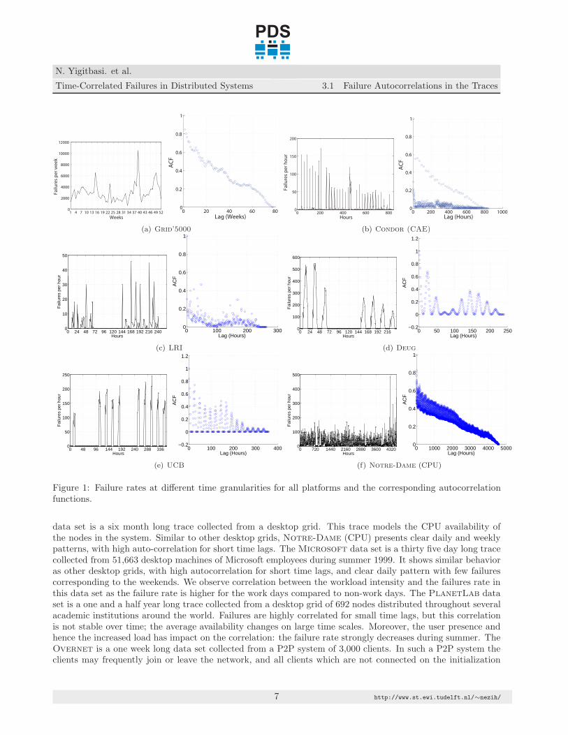
1 Failure rates at different time granularities for all platforms and the corresponding autocorrelationfunctions. . . . . . . . . . . . . . . . . . . . . . . . . . . . . . . . . . . . . . . . . . . . . . . . . . 7

2 Failure rates at different time granularities for all platforms and the corresponding autocorrelationfunctions (Cont.). . . . . . . . . . . . . . . . . . . . . . . . . . . . . . . . . . . . . . . . . . . . . . 8



5 Daily and hourly failure rates for Overnet,Grid’5000,Notre-Dame (CPU), and PlanetLabplatforms. . . . . . . . . . . . . . . . . . . . . . . . . . . . . . . . . . . . . . . . . . . . . . . . . 12

6 Parameters of the peak periods model. The numbers in the figure match the (numbered) modelparameters in the text. . . . . . . . . . . . . . . . . . . . . . . . . . . . . . . . . . . . . . . . . . . 13

7 Peak Duration: CDF of the empirical data for the Notre-Dame (CPU) platform and thedistributions investigated for modeling the peak duration parameter. None of the distributionsprovide a good fit due to a peak at 1h. . . . . . . . . . . . . . . . . . . . . . . . . . . . . . . . . . 17

List of Tables

1 Summary of nineteen data sets in the Failure Trace Archive. . . . . . . . . . . . . . . . . . . . . . 52 Average values for the model parameters. . . . . . . . . . . . . . . . . . . . . . . . . . . . . . . . 143 Empirical distribution for the peak duration parameter. . . . . . . . . . . . . . . . . . . . . . . . 154 Peak model: The parameter values for the best fitting distributions for all studied systems. . . 165 The average duration and average IAT of failures for the entire traces and for the peaks. . . . . . 166 Fraction of downtime and fraction of number of failures due to failures that originate during

peaks (k = 1). . . . . . . . . . . . . . . . . . . . . . . . . . . . . . . . . . . . . . . . . . . . . . . . 17




PDS

Wp

Wp1. Introduction

1 Introduction

Large-scale distributed systems have reached an unprecedented scale and complexity in recent years. At thisscale failures inevitably occur—networks fail, disks crash, packets get lost, bits get flipped, software misbehaves,or systems crash due to misconfiguration and other human errors. Deadline-driven or mission-critical servicesare part of the typical workload for these infrastructures, which thus need to be available and reliable despitethe presence of failures. Researchers and system designers have already built numerous fault-tolerance mecha-nisms that have been proven to work under various assumptions about the occurrence and duration of failures.However, most previous work focuses on failure models that assume the failures to be non-correlated, but thismay not be realistic for the failures occurring in large-scale distributed systems. For example, such systemsmay exhibit peak failure periods, during which the failure rate increases, affecting in turn the performance offault-tolerance solutions. To investigate such time correlations, we perform in this work a detailed investiga-tion of the time-varying behavior of failures using nineteen traces obtained from several large-scale distributedsystems including grids, P2P systems, DNS servers, web servers, and desktop grids.

Recent studies report that in production systems, failure rates can be of over 1000 failures per year and,depending on the root cause of the corresponding problems, the mean time to repair can range from hoursto days [16]. The increasing scale of deployed distributed systems causes the failure rates to increase, whichin turn can have a significant impact on the performance and cost, such as degraded response times [21] andincreased Total Cost of Operation (TCO) due to increased administration costs and human resource needs [1].This situation also motivates the need for further research in failure characterization and modeling.

Previous studies [18,13,12,14,20,16] focused on characterizing failures in several different distributed systems.However, most of these studies assume that failures occur independently or disregard the time correlation offailures, despite the practical importance of these correlations [11, 19, 15]. First of all, understanding if failuresare time correlated has significant implications for proactive fault tolerance solutions. Second, understandingthe time-varying behavior of failures and peaks observed in failure patterns is required for evaluating designdecisions. For example, redundant submissions may all fail during a failure peak period, regardless of the qualityof the resubmission strategy. Third, understanding the temporal correlations and exploiting them for smartcheckpointing and scheduling decisions provides new opportunities for enhancing conventional fault-tolerancemechanisms [21,7]. For example, a simple scheduling policy could be to stop scheduling large parallel jobs duringfailure peaks. Finally, it is possible to devise adaptive fault-tolerance mechanisms that adjust the policies basedon the information related to peaks. For example, an adaptive fault-tolerance mechanism can migrate thecomputation at the beginning of a predicted peak.

To understand the time-varying behavior of failures in large-scale distributed systems, we perform a detailedinvestigation using data sets from diverse large-scale distributed systems including more than 100K hosts and1.2M failure events spanning over 15 years of system operation. Our main contribution is threefold:

1. We make four new failure traces publicly available through the Failure Trace Archive (Section 2).

2. We present a detailed evaluation of the time correlation of failure events observed in traces taken fromnineteen (production) distributed systems (Section 3).

3. We propose a model for peaks observed in the failure rate process (Section 4).

2 Method

2.1 Failure Datasets

In this work we use and contribute to the data sets in the Failure Trace Archive (FTA) [9]. The FTA is anonline public repository of availability traces taken from diverse parallel and distributed systems.

The FTA makes failure traces available online in a unified format, which records the occurrence time andduration of resource failures as an alternating time series of availability and unavailability intervals. Each




PDS

Wp

Wp2.2 Analysis

Table 1: Summary of nineteen data sets in the Failure Trace Archive.

System Type Nodes Period Year EventsGrid’5000 Grid 1,288 1.5 years 2005-2006 588,463COND-CAE1 Grid 686 35 days 2006 7899COND-CS1 Grid 725 35 days 2006 4543COND-GLOW1 Grid 715 33 days 2006 1001TeraGrid Grid 1001 8 months 2006-2007 1999LRI Desktop Grid 237 10 days 2005 1,792Deug Desktop Grid 573 9 days 2005 33,060Notre-Dame 2 Desktop Grid 700 6 months 2007 300,241Notre-Dame 3 Desktop Grid 700 6 months 2007 268,202Microsoft Desktop Grid 51,663 35 days 1999 1,019,765UCB Desktop Grid 80 11 days 1994 21,505PlanetLab P2P 200-400 1.5 year 2004-2005 49,164Overnet P2P 3,000 2 weeks 2003 68,892Skype P2P 4,000 1 month 2005 56,353Websites Web servers 129 8 months 2001-2002 95,557LDNS DNS servers 62,201 2 weeks 2004 384,991SDSC HPC Clusters 207 12 days 2003 6,882LANL HPC Clusters 4,750 9 years 1996-2005 43,325PNNL HPC Cluster 1,005 4 years 2003-2007 4,6501COND-* data sets denote the Condor data sets.

2This is the host availability version which is according to the multi-state availability model of Brent Rood.

3This is the CPU availability version.

availability or unavailability event in a trace records the start and the end of the event, and the resource thatwas affected by the event. Depending on the trace, the resource affected by the event can be either a node of adistributed system such as a node in a grid, or a component of a node in a system such as CPU or memory.

Prior to the work leading to this article, the FTA made fifteen failure traces available in its standardformat; as a result of our work, the FTA now makes available nineteen failure traces. Table 1 summarizesthe characteristics of these nineteen traces, which we use throughout this work. The traces originate fromsystems of different types (multi-cluster grids, desktop grids, peer-to-peer systems, DNS and web servers) andsizes (from hundreds to tens of thousands of resources), which makes these traces ideal for a study amongdifferent distributed systems. Furthermore, many of the traces cover several months of system operation. Amore detailed description of each trace is available on the FTA web site(http://fta.inria.fr).

2.2 Analysis

In our analysis, we use the autocorrelation function (ACF) to measure the degree of correlation of the failuretime series data with itself at different time lags. The ACF takes on values between -1 (high negative correlation)and 1 (high positive correlation). In addition, the ACF reveals when the failures are random or periodic. Forrandom data the correlation coefficients will be close to zero; and a periodic component in the ACF reveals thatthe failure data is periodic or at least it has a periodic component.

2.3 Modeling

In the modeling phase, we statistically model the peaks observed in the failure rate process, i.e., the number offailure events per time unit. Towards this end we use the Maximum Likelihood Estimation (MLE) method [2]for fitting the probability distributions to the empirical data as it delivers good accuracy for the large data


http://fta.inria.fr



PDS

Wp

Wp3. Analysis of Autocorrelation

samples specific to failure traces. After we determine the best fits for each candidate distribution for all datasets, we perform the goodness-of-fit tests to assess the quality of the fitting for each distribution, and to establishthe best fit. As the goodness-of-fit tests, we use both the Kolmogorov-Smirnov (KS) and the Anderson-Darling(AD) tests, which essentially assess how close the cumulative distribution function (CDF) of the probabilitydistribution is to the CDF of the empirical data. For each candidate distribution with the parameters foundduring the fitting process, we formulate the hypothesis that the empirical data are derived from it (the null-hypothesis of the goodness-of-fit test). Neither the KS or the AD tests can confirm the null-hypothesis, but bothare useful in understanding the goodness-of-fit. For example, the KS-test provides a test statistic, D, whichcharacterizes the maximal distance between the CDF of the empirical distribution of the input data and thatof the fitted distribution; distributions with a lower D value across different failure traces are better. Similarly,the tests return p-values which are used to either reject the null-hypothesis if the p-value is smaller than orequal to the significance level, or confirm that the observation is consistent with the null-hypothesis if the p-value is greater than the significance level. Consistent with the standard method for computing p-values [12,9],we average 1,000 p-values, each of which is computed by selecting 30 samples randomly from the data set, tocalculate the final p-value for the goodness-of-fit tests.

3 Analysis of Autocorrelation

In this section we present the autocorrelations in failures using traces obtained from grids, desktop grids, P2Psystems, web servers, DNS servers and HPC clusters, respectively. We consider the failure rate process, that isthe number of failure events per time unit.

3.1 Failure Autocorrelations in the Traces

Our aim is to investigate whether the occurrence of failures is repetitive in our data sets. Toward this end,we compute the autocorrelation of the failure rate for different time lags including hours, weeks, and months.Figure 1 shows for several platforms the failure rate at different time granularities, and the correspondingautocorrelation functions. Overall, we find that many systems exhibit strong correlation from small to moderatetime lags confirming that failures are indeed repetitive in many of the systems.

Many of the systems investigated in this work exhibit strong autocorrelation for hourly and weekly lags.Figures 1(a), 1(b), 1(c), 1(d), 1(e), 1(f), 2(a), 2(b), 2(c), 2(d), 2(e), 2(f), 3(a), 3(b), and 3(c) show thefailure rates and autocorrelation functions for the Grid’5000, Condor (CAE), LRI, Deug, UCB, Notre-Dame (CPU), Microsoft, PlanetLab, Overnet, Skype, Websites, LDNS, SDSC, and LANL systems,respectively.

The Grid’5000 data set is a one and a half year long trace collected from an academic research grid. Sincethis system is mostly used for experimental purposes, and is large-scale (∼3K processors) the failure rate isquite high. In addition, since most of the jobs are submitted through the OAR resource manager, hence withoutdirect user interaction, the daily pattern is not clearly observable. However, during the summer the failure ratedecreases, which indicates a correlation between the system load and the failure rate. Finally, as the systemsize increases over the years, the failure rate does not increase significantly, which indicates system stability.The Condor (CAE) data set is a one month long trace collected from a desktop grid using the Condor cycle-stealing scheduler. As expected from a desktop grid, this trace exhibits daily peaks in the failure rate, andhence in the autocorrelation function. In contrast to other desktop grids, the failure rate is lower. The LRIdata set is a ten day long trace collected from a desktop grid. The main trend of this trace is enforced byusers who power their machines off during weekends. Deug and UCB data sets are nine and eleven day longtraces collected from desktop grids. In contrast to LRI, machines in these systems are shut down every night.This difference is captured well by autocorrelation functions: LRI has moderate peaks for lags correspondingto one or two days, while a clear daily pattern is visible in Deug and UCB systems. The Notre-Dame (CPU)




PDS

Wp

Wp3.1 Failure Autocorrelations in the Traces

1 4 7 10 13 16 19 22 25 28 31 34 37 40 43 46 49 520

2000

4000

6000

8000

10000

12000

Fa

ilu

res

pe

r w

ee

k

Weeks

0 20 40 60 800

0.2

0.4

0.6

0.8

1

Lag (Weeks)

AC

F

(a) Grid’5000

0 200 400 600 8000

50

100

150

200

Fa

ilu

res

pe

r h

ou

r

Hours0 200 400 600 800 1000

0

0.2

0.4

0.6

0.8

1

Lag (Hours)

AC

F

(b) Condor (CAE)

0 24 48 72 96 120 144 168 192 216 2400

10

20

30

40

50

Fai

lure

s pe

r ho

ur

Hours0 100 200 300

0

0.2

0.4

0.6

0.8

1

Lag (Hours)

AC

F

(c) LRI

0 24 48 72 96 120 144 168 192 2160

100

200

300

400

500

600

Fai

lure

s pe

r ho

ur

Hours0 50 100 150 200 250

−0.2

0

0.2

0.4

0.6

0.8

1

1.2

Lag (Hours)

AC

F

(d) Deug

0 48 96 144 192 240 288 3360

50

100

150

200

250

Fai

lure

s pe

r ho

ur

Hours0 100 200 300 400

−0.2

0

0.2

0.4

0.6

0.8

1

1.2

Lag (Hours)

AC

F

(e) UCB

0 720 1440 2160 2880 3600 43200

100

200

300

400

500

Fai

lure

s pe

r ho

ur

Hours0 1000 2000 3000 4000 5000

0

0.2

0.4

0.6

0.8

1

Lag (Hours)

AC

F

(f) Notre-Dame (CPU)

Figure 1: Failure rates at different time granularities for all platforms and the corresponding autocorrelationfunctions.

data set is a six month long trace collected from a desktop grid. This trace models the CPU availability ofthe nodes in the system. Similar to other desktop grids, Notre-Dame (CPU) presents clear daily and weeklypatterns, with high auto-correlation for short time lags. The Microsoft data set is a thirty five day long tracecollected from 51,663 desktop machines of Microsoft employees during summer 1999. It shows similar behavioras other desktop grids, with high autocorrelation for short time lags, and clear daily pattern with few failurescorresponding to the weekends. We observe correlation between the workload intensity and the failures rate inthis data set as the failure rate is higher for the work days compared to non-work days. The PlanetLab dataset is a one and a half year long trace collected from a desktop grid of 692 nodes distributed throughout severalacademic institutions around the world. Failures are highly correlated for small time lags, but this correlationis not stable over time; the average availability changes on large time scales. Moreover, the user presence andhence the increased load has impact on the correlation: the failure rate strongly decreases during summer. TheOvernet is a one week long data set collected from a P2P system of 3,000 clients. In such a P2P system theclients may frequently join or leave the network, and all clients which are not connected on the initialization




PDS

Wp


0 200 400 600 8000

2000

4000

6000

8000

10000

12000

Fai

lure

s pe

r ho

ur

Hours0 200 400 600 800 1000

0

0.2

0.4

0.6

0.8

1

Lag (Hours)

AC

F

(a) Microsoft

0 10 20 30 40 50100

200

300

400

500

600

700

Fai

lure

s pe

r w

eek

Weeks0 10 20 30 40 50

0

0.2

0.4

0.6

0.8

1

Lag (Weeks)

AC

F

(b) PlanetLab

0 24 48 72 96 120 144 1680

500

1000

1500

2000

Fai

lure

s pe

r ho

ur

Hours0 50 100 150 200

0

0.2

0.4

0.6

0.8

1

Lag (Hours)

AC

F

(c) Overnet

0 200 400 6000

100

200

300

400

500

Fa

ilu

res

pe

r h

ou

r

Hours

0 200 400 600 8000

0.2

0.4

0.6

0.8

1

Lag (Hours)

AC

F

(d) Skype

0 1000 2000 3000 4000 50000

50

100

150

200

Fai

lure

s pe

r ho

ur

Hours0 2000 4000 6000

0

0.2

0.4

0.6

0.8

1

Lag (Hours)

AC

F

(e) Websites (hourly)

0 10 20 30 400

500

1000

1500

2000

2500

3000

Fai

lure

s pe

r w

eek

Weeks0 10 20 30 40

0

0.2

0.4

0.6

0.8

1

Lag (Weeks)

AC

F

(f) Websites (weekly)

Figure 2: Failure rates at different time granularities for all platforms and the corresponding autocorrelationfunctions (Cont.).




PDS

Wp


0 48 96 144 192 240 288 336 384 432 480 528 5760

200

400

600

800

Fa

ilu

res

pe

r h

ou

r

Hours

0 200 400 6000

0.2

0.4

0.6

0.8

1

Lag (Hours)

AC

F

(a) LDNS

0 24 48 72 96 1201441681922162402642880

50

100

150

200

250

Fai

lure

s pe

r ho

ur

Hours0 100 200 300 400

0

0.2

0.4

0.6

0.8

1

Lag (Hours)

AC

F

(b) SDSC

1 4 7 10 13 16 19 22 25 28 31 34 37 40 43 46 49 5220

40

60

80

100

120

Fa

ilu

res

pe

r w

ee

k

Weeks1 4 7 10 13 16 19 22 25 28 31 34 37 40 43 46 49 52

40

60

80

100

120

140

Fa

ilu

res

pe

r w

ee

k

Weeks0 50 100 150

0

200

400

600

800F

ail

ure

s p

er

mo

nth

Months

(c) LANL (For 2002, 2004 and the whole trace)

0 20 40 600

0.2

0.4

0.6

0.8

1

Lag (Weeks)

AC

F

0 20 40 600

0.2

0.4

0.6

0.8

1

Lag (Weeks)

AC

F

0 50 100 1500

0.2

0.4

0.6

0.8

1

Lag (Months)

AC

F

(d) LANL (For 2002, 2004 and the whole trace)





PDS

Wp


0 1000 2000 3000 4000 5000 60000

10

20

30

40

50

Fa

ilu

res

pe

r h

ou

r

Hours

0 2000 4000 6000 80000

0.2

0.4

0.6

0.8

1

Lag (Hours)

AC

F

(a) TeraGrid

0 720 1440 2160 2880 3600 43200

100

200

300

400

Fa

ilu

res

pe

r h

ou

r

Hours

0 1000 2000 3000 4000 50000

0.2

0.4

0.6

0.8

1

Lag (Hours)

AC

F

(b) Notre-Dame

0 0.432 0.864 1.296 1.728 2.16 2.592

x 104

0

10

20

30

40

Fai

lure

s pe

r ho

ur

Hours0 1 2 3

x 104

0

0.2

0.4

0.6

0.8

1

Lag (Hours)

AC

F

(c) PNNL (hourly)


are considered as down, explaining the initial peak of failures. We observe strong autocorrelation for short timelags similar to other P2P systems. The Skype data set is a one month long trace collected from a P2P systemused by 4, 000 clients. Similar to Overnet, clients of Skype may also join or leave the system, and clients thatare not online are considered as unavailable in this trace. Similar to desktop grids, there is high autocorrelationat small time lags, and the daily and weekly peaks are more pronounced. The Websites data set is a sevenmonth long trace collected from web servers. While the average availability of the web servers remains almoststable (around 80%), there are few peaks in the failure rate probably due to network problems. In addition,we do not observe clear hourly and weekly patterns. The LDNS data set is a two week long trace collectedfrom DNS servers. Unlike P2P systems and desktop grids, DNS servers do not exhibit strong autocorrelationfor short time lags with periodic behavior. In addition, as the workload intensity increases during the peakhours of the day, we observe that the failure rate also increases. The SDSC data set is a twelve day long tracecollected from the San Diego Supercomputer Center (HPC clusters). Similar to other HPC clusters and grids,we observe strong correlation for small to moderate time lags. Finally, The LANL data set is a ten year longtrace collected from production HPC clusters. The weekly failure rate is quite low compared to Grid’5000.We do not observe a clear yearly pattern as the failure rate increases during summer 2002, whereas the failurerate decreases during summer 2004. Since around 3, 000 nodes were added to the LANL system between 2002and 2003, the failure rate also increases correspondingly.

Last, a few systems exhibit weak autocorrelation in failure occurrence. Figure 4(a), 4(b), and 4(c) showthe failure rate and the corresponding autocorrelation function for the TeraGrid, Notre-Dame and PNNLsystems. The TeraGrid data set is an eight month long trace collected from an HPC cluster that is part ofa grid. We observe weak autocorrelation at all time lags, which implies that the failure rates observed overtime are independent. In addition, there are no clear hourly or daily patterns, which gives evidence of anerratic occurrence of failures in this system. The Notre-Dame data set is a six month long trace collected




PDS

Wp

Wp3.2 Discussion

from a desktop grid. The failure events in this data set consist of the availability/unavailability events of thehosts in this system. Similar to other desktop grids, we observe clear daily and weekly patterns. However,the autocorrelation is low when compared to other desktop grids. Finally, PNNL data set is a four year longtrace collected from HPC clusters. We observe correlation between the intensity of the workload and the hourlyfailure rate since the failure rate decreases during the summer. The weak autocorrelation indicates independentfailures as expected from HPC clusters.

3.2 Discussion

As we have shown in the previous section, many systems exhibit strong correlation from small to moderatetime lags, which indicates probably a high degree of predictability. In contrast, a small number of systems(Notre-Dame, PNNL, and TeraGrid) exhibit weak autocorrelation; only for these systems, the failure ratesobserved over time are independent.

We have found that similar systems have similar time-varying behavior, e.g., desktop grids and P2P systemshave daily and weekly periodic failure rates, and these systems exhibit strong temporal correlation at hourlytime lags. Some systems (Notre-Dame and Condor (CAE)) have direct user interaction, which producesclear daily and weekly patterns in both system load and occurrence of failures—the failure rate increases duringwork hours and days, and decreases during free days and holidays (the summer).

Finally, not all systems exhibit a correlation between work hours and days, and the failure rate. In theexamples depicted in Figure 5, while Grid’5000 exhibits this correlation, PlanetLab exhibit irregular/erratichourly and daily failure behavior.

Our results are consistent with previous studies [14, 4, 8, 17] as in many traces we observe strong autocor-relation at small time lags, and that we observe correlation between the intensity of the workload and failurerates.

4 Modeling the Peaks of Failures

In this section we present a model for the peaks observed in the failure rate process in diverse large-scaledistributed systems.

4.1 Peak Periods Model

Our model of peak failure periods comprises four parameters as shown in Figure 6: the peak duration, the timebetween peaks (inter-peak time), the inter-arrival time of failures during peaks, and the duration of failuresduring peaks:

1. Peak Duration: The duration of peaks observed in a data set.

2. Time Between Peaks (inter-peak time): The time from the end of a previous peak to the start ofthe next peak.

3. Inter-arrival Time of Failures During Peaks: The inter-arrival time of failure events that occurduring peaks.

4. Failure Duration During Peaks: The duration of failure events that start during peaks. These failureevents may last longer than a peak.

Our modeling process is based on analyzing the failure traces taken from real distributed systems in twosteps which we describe in turn.




PDS

Wp

Wp4.1 Peak Periods Model

4200

4400

4600

4800

5000

5200

5400

5600

5800

6000

6200

6400

Friday MondaySaturdaySundayThursdayTuesdayWednesday

Nu

mb

er

of

Fa

ilure

s

Day of Week

1000

1500

2000

2500

3000

3500

0 1 2 3 4 5 6 7 8 9 1011121314151617181920212223

Nu

mb

er

of

Fa

ilure

s

Hour of Day

(a) Overnet

20000

25000

30000

35000

40000

45000

50000

55000

Mon Tue Wed Thu Fri Sat Sun

Nu

mb

er

of

Fa

ilure

s

Day of Week

2000

4000

6000

8000

10000

12000

14000

16000

18000

20000

22000

0 1 2 3 4 5 6 7 8 9 1011121314151617181920212223

Nu

mb

er

of

Fa

ilure

s

Hour of Day

(b) Grid’5000

10000

12000

14000

16000

18000

20000

22000

24000

Friday MondaySaturdaySundayThursdayTuesdayWednesday

Nu

mb

er

of

Fa

ilure

s

Day of Week

1000

2000

3000

4000

5000

6000

7000

8000

9000

10000

11000

0 1 2 3 4 5 6 7 8 9 1011121314151617181920212223

Nu

mb

er

of

Fa

ilure

s

Hour of Day

(c) Notre-Dame (CPU)

2600

2800

3000

3200

3400

3600

3800

4000

4200

Mon Tue Wed Thu Fri Sat Sun

Nu

mb

er

of

Fa

ilure

s

Day of Week

800

900

1000

1100

1200

1300

1400

1500

0 1 2 3 4 5 6 7 8 9 1011121314151617181920212223

Nu

mb

er

of

Fa

ilure

s

Hour of Day

(d) PlanetLab

Figure 5: Daily and hourly failure rates for Overnet,Grid’5000,Notre-Dame (CPU), and PlanetLabplatforms.




PDS

Wp

Wp4.2 Results

Fa

ilu

re

Ra

te

Time

Failure Rate

Peak

Failure Event

1 1 12 2 2 2

3

44

Figure 6: Parameters of the peak periods model. The numbers in the figure match the (numbered) modelparameters in the text.

The first step is to identify for each trace the peaks of hourly failure rates. Since there is no rigorousmathematical definition of peaks in time-series, to identify the peaks we define a threshold value as µ + kσ,where µ is the average and σ is the standard deviation of the failure rate, and k is a positive integer; a periodwith a failure rate above the threshold is a peak period. We adopt this threshold to achieve a good balancebetween capturing in the model extreme system behavior, and characterizing with our model an important partof the system failures (either number of failures or downtime caused to the system). A threshold excluding allbut a few periods, for example defining peak periods as distributional outliers, may capture too few periods andexplain only a small fraction of the system failures. A more inclusive threshold would lead to the inclusion ofmore failures, but the data may come from periods with very different characteristics, which is contrary to thegoal of building a model for peak failure periods.

In the second step we extract the model parameters from the data sets using the peaks that we identified inthe first step. Then we try to find a good fit, that is, a well-known probability distribution and the parametersthat lead to the best fit between that distribution and the empirical data. When selecting the probabilitydistributions, we consider the degrees of freedom (number of parameters) of that distribution. Although adistribution with more degrees of freedom may provide a better fit for the data, such a distribution can resultin a complex model, and hence it may be difficult to analyze the model mathematically. In this study we usefive probability distributions to fit to the empirical data: exponential, Weibull, Pareto, lognormal, and gamma.For the modeling process, we follow the methodology that we describe in Section 2.3.

4.2 Results

After applying the modeling methodology that we describe in the previous section and Section 2.3, in thissection we present the peak model that we derived from diverse large scale distributed systems.

Table 2 shows the average values for all the model parameters for all platforms. The average peak duration




PDS

Wp

Wp4.2 Results

Table 2: Average values for the model parameters.

System Avg. Peak Avg. Failure Avg. Time Avg. FailureDuration [s] IAT During Between Peaks [s] Duration During

Peaks [s] Peaks [s]

Grid’5000 5,047 13 55,101 20,984Condor (CAE) 5,287 23 87,561 4,397Condor (CS) 3,927 4 241,920 20,740

Condor (GLOW) 4,200 14 329,040 75,672TeraGrid 3,680 35 526,500 368,903

LRI 4,080 78 58,371 31,931Deug 14,914 10 103,800 1,091

Notre-Dame 3,942 21 257,922 280,593Notre-Dame (CPU) 7,520 33 47,075 22,091

Microsoft 7,200 0 75,315 90,116UCB 21,272 23 77,040 332

PlanetLab 4,810 264 47,124 166,913Overnet 3,600 1 14,400 382,225Skype 4,254 11 112,971 26,402

Websites 5,211 103 104,400 3476LDNS 4,841 8 42,042 30,212SDSC 4,984 26 84,900 6,114LANL 4,122 653 94,968 21,193

varies across different systems, and even for the same type of systems. For example, UCB, Microsoft andDeug are all desktop grids, but the average peak duration widely varies among these platforms. In contrast,for the SDSC, LANL, and PNNL platforms, which are HPC clusters, the average peak duration values arerelatively close. The Deug and UCB platforms have small number of long peak durations resulting in higheraverage peak durations compared to the other platforms. Finally, as there are two peaks of zero length (singledata point) in the Overnet system, the average peak duration is zero.

The average inter-arrival time during peaks is rather low, as expected, as the failure rates are higher duringpeaks compared to off-peak periods. For the Microsoft platform, as all failures arrive as burst during peaks,average inter-arrival time during peaks is zero.

Similar to the average peak duration parameter, the average time between peaks parameter is also highlyvariable across different systems. For some systems like TeraGrid, this parameter is in the order of days, andfor some systems like Overnet it is in the order of hours.

Similarly, the duration of failures during peaks highly varies even across similar platforms. For example, thedifference between the average failure duration during peaks between the UCB and the Microsoft platforms,which are both desktop grids, is huge because the machines in the UCB platform leave the system less oftenthan the machines in the Microsoft platform. In addition, in some platforms like Overnet and TeraGrid,the average failure durations during peaks is in the order of days showing the impact of space-correlated failures,that is multiple nodes failing nearly simultaneously.

Using the AD and KS tests we next determine the best fitting distributions for each model parameter andeach system. Since we determine the hourly failure rates using fixed time windows of one hour, the peak durationand the inter-peak time are multiples of one hour. In addition, as the peak duration parameter is mostly inthe range [1h-5h], and for several systems this parameter is mostly 1h causing the empirical distribution tohave a peak at 1h, none of the distributions provide a good fit for the peak duration parameter (see Figure 7).Therefore, for the peak duration model parameter, we only present an empirical histogram in Table 3. We find




PDS

Wp

Wp4.2 Results

Table 3: Empirical distribution for the peak duration parameter. h denotes hours. Values above 10% aredepicted as bold.

Platform / Peak Duration 1h 2h 3h 4h 5h 6h ≥ 7h

Grid’5000 80.56 % 13.53 % 3.38 % 1.33 % 0.24 % 0.12 % 0.84%Condor (CAE) 93.75 % 3.13 % – – – – 3.12%Condor (CS) 90.91 % 9.09 % – – – – –

Condor (GLOW) 83.33 % 16.67 % – – – – –TeraGrid 97.78 % 2.22 % – – – – –

LRI 86.67 % 13.33 % – – – – –Deug 28.57 % – 28.57 % – 14.29 % – 28.57 %

Notre-Dame 90.48 % 9.52 % – – – – –Notre-Dame (CPU) 56.83 % 17.78 % 9.84 % 3.49 % 5.40 % 3.49 % 3.17

Microsoft 35.90 % 33.33 % 25.64 % 5.13 % – – –UCB 9.09 % 9.09 % – – – 9.09 % 72.73 %

PlanetLab 80.17 % 13.36 % 3.71 % 1.27 % 0.53 % 0.53 % 0.43Overnet 100.00 % – – – – – –Skype 90.91 % 4.55 % – 4.55 % – – –

Websites 76.74 % 13.95 % 5.23 % 2.33 % 0.58 % – 1.16LDNS 75.86 % 13.79 % 10.34 % – – – –SDSC 69.23 % 23.08 % 7.69 % – – – –LANL 88.35 % 9.24 % 2.06 % 0.25 % 0.06 % 0.03 % –PNNL 85.99 % 10.35 % 1.75 % 0.96 % 0.64 % 0.16 % 0.16 %

Avg 74.79 % 11.3 % 5.16 % 1.01 % 1.14 % 0.7 % 5.85 %

that the peak duration for almost all platforms are less than 3h.Table 4 shows the best fitting distributions for the model parameters for all data sets investigated in this

study. To generate synthetic yet realistic traces without using a single system as a reference, we create theaverage system model which has the average characteristics of all systems we investigate. We create the averagesystem model as follows. First, we determine the candidate distributions for a model parameter with thedistributions having the smallest D values for each system. Then, for each model parameter, we determinethe best fitting distribution among the candidate distributions that has the lowest average D value over alldata sets. After we determine the best fitting distribution for the average system model, each data set is fitindependently to this distribution to find the set of best fit parameters. The parameters of the average systemmodel shown in the ”Avg.” row represent the average of this set of parameters.

For the IAT during peak durations, several platforms do not have a best fitting distribution since for theseplatforms most of the failures during peaks occur as bursts hence having inter-arrival times of zero. Similarly,for the time between peaks parameter, some platforms (like all CONDOR platforms, Deug, Overnet andUCB platforms) do not have best fitting distributions since these platforms have inadequate number of samplesto generate a meaningful model. For the failure duration between peaks parameter, some platforms do not havea best fitting distribution due to the nature of the data. For example, for all CONDOR platforms the failureduration is a multiple of a monitoring interval creating peaks in the empirical distribution at that monitoringinterval. As a result, none of the distributions we investigate provide a good fit.

In our model we find that the model parameters do not follow a heavy-tailed distribution since the p-valuesfor the Pareto distribution are very low. For the IAT during peaks parameter, Weibull distribution providesa good fit for most of the platforms. For the time between peaks parameter, we find that the platforms caneither be modeled by the lognormal distribution or the Weibull distribution. Similar to our previous model [9],which is derived from both peak and off-peak periods, for the failure duration during peaks parameter, we findthat the lognormal distribution provides a good fit for most of the platforms. To conclude, for all the modelparameters, we find that either the lognormal or the Weibull distributions provide a good fit for the averagesystem model.

Similar to the average system models built for other systems [10], we cannot claim that our average systemmodel represents the failure behavior of an actual system. However, the main strength of the average systemmodel is that it represents a common basis for the traces from which it has been extracted. To generate failure




PDS

Wp

Wp5. Related Work

Table 4: Peak model: The parameter values for the best fitting distributions for all studied systems. E,W,LN,and G stand for exponential, Weibull, lognormal and gamma distributions, respectively.

System IAT During Peaks Time Between Peaks Failure Duration During Peaks

Grid’5000 – (see text) LN(10.30,1.09) – (see text)Condor (CAE) – (see text) – (see text) – (see text)Condor (CS) – (see text) – (see text) – (see text)

Condor (GLOW) – (see text) – (see text) – (see text)TeraGrid – (see text) LN(12.40,1.42) LN(10.27,1.90)

LRI LN(3.49,1.86) LN(10.51,0.98) – (see text)Deug W(9.83,0.95) – (see text) LN(5.46,1.29)

Notre-Dame – (see text) W(247065.52,0.92) LN(9.06,2.73)Notre-Dame (CPU) – (see text) W(44139.20,0.89) LN(7.19,1.35)

Microsoft – (see text) G(1.50,50065.81) W(55594.48,0.61)UCB E(23.77) – (see text) LN(5.25,0.99)

PlanetLab – (see text) LN(10.13,1.03) LN(8.47,2.50)Overnet – (see text) – (see text) – (see text)Skype – (see text) W(123440.05,1.37) – (see text)

Websites W(66.61,0.60) LN(10.77,1.25) – (see text)LDNS W(8.97,0.98) LN(10.38,0.79) LN(9.09,1.63)SDSC W(16.27,0.46) E(84900) LN(7.59,1.68)LANL G(1.35,797.42) LN(10.63,1.16) LN(8.26,1.53)PNNL – (see text) E(160237.32) – (see text)

Avg W(193.91,0.83) LN(10.89,1.08) LN(8.09,1.59)

Table 5: The average duration and average IAT of failures for the entire traces and for the peaks.

System Avg. Failure Avg. Failure Avg. Failure Avg. FailureDuration [h] Duration [h] IAT [s] IAT [s]

(Entire) (Peaks) (Entire) (Peaks)

Grid’5000 7.41 5.83 160 13Notre-Dame (CPU) 4.25 6.14 119 33

Microsoft 16.49 25.03 6 0PlanetLab 49.61 46.36 1880 264Overnet 11.98 106.17 17 1Skype 14.30 7.33 91 11

Websites 1.17 0.97 380 103LDNS 8.61 8.39 12 8LANL 5.88 5.89 13874 653

traces for a specific system, individual best fitting distributions and their parameters shown in Table 4 may beused instead of the average system.

Next, we compute the average failure duration/inter-arrival time over each data set and only during peaks(Table 5). We compare only the data sets used both in this study and our previous study [9], where we modelledeach data set individually without isolating peaks. We observe that the average failure duration per data setcan be twice as long as the average duration during peaks. In addition, the average failure inter-arrival timeper data set is on average nine times the average failure inter-arrival time during peaks. This implies thatthe distribution per data set is significantly different from the distribution for peaks, and that fault detectionmechanisms must be significantly faster during peaks. Likewise, fault-tolerance mechanisms during peaks musthave considerably lower overhead than during non-peak periods.

Finally, we investigate the fraction of downtime caused by failures that originate during peaks, and thefraction of the number of failures that originate during peaks (Table 6). We find that on average over 50% andup to 95% of the downtime of the systems we investigate are caused by the failures that originate during peaks.

5 Related Work

Much work has been dedicated to characterizing and modeling system failures [18, 13, 12, 14, 20, 16]. Whilethe correlation among failure events has received attention since the early 1990s [18], previous studies focusmostly on space-correlated failures, that is, on multiple nodes failing nearly simultaneously. Although the time




PDS

Wp

Wp5. Related Work

0 0.5 1 1.5 2 2.5 3 3.5 4

x 104

0

0.1

0.2

0.3

0.4

0.5

0.6

0.7

0.8

0.9

1

CD

F

Peak Duration (seconds)

Empirical data

Exp

Weibull

G−Pareto

LogN

Gamma

Figure 7: Peak Duration: CDF of the empirical data for the Notre-Dame (CPU) platform and the distri-butions investigated for modeling the peak duration parameter. None of the distributions provide a good fitdue to a peak at 1h.

Table 6: Fraction of downtime and fraction of number of failures due to failures that originate during peaks.System k = 0.5 k = 0.9 k = 1.0 k = 1.1 k = 1.25 k = 1.5 k = 2.0

Time % # Failures % Time % # Failures % Time % # Failures % Time % # Failures % Time % # Failures % Time % # Failures % Time % # Failures %

Grid’5000 61.93 74.43 52.11 64.58 49.19 62.56 47.27 60.84 35.93 57.93 33.25 53.60 27.63 44.99Condor (CAE) 63.03 90.91 62.93 90.52 62.93 90.52 62.73 89.88 62.73 89.88 62.57 89.13 62.10 87.08Condor (CS) 80.09 89.56 80.04 88.63 80.04 88.63 80.04 88.63 80.04 88.63 80.04 88.63 80.04 88.63

Condor (GLOW) 39.53 70.51 39.37 69.70 39.37 69.70 39.37 69.70 39.37 69.70 39.37 69.70 37.28 67.47TeraGrid 100 77.10 66.90 77.10 66.90 77.10 66.90 77.10 66.90 77.10 66.90 77.10 62.98 70.61

LRI 87.42 71.87 84.73 62.26 84.73 62.26 77.92 59.47 75.66 57.94 75.66 57.94 73.91 55.71Deug 47.31 83.61 26.07 66.46 25.07 63.03 25.07 63.03 22.28 57.76 20.94 53.31 16.83 41.11

Notre-Dame 62.62 73.06 58.53 69.72 53.40 69.09 45.19 67.70 45.12 67.19 43.69 64.47 41.79 62.61Notre-Dame (CPU) 73.77 56.92 63.85 43.56 57.92 40.15 56.19 37.93 47.61 33.32 41.88 26.21 28.76 14.99

Microsoft 52.16 40.26 37.44 25.10 35.54 23.41 32.20 20.08 28.78 16.81 23.76 12.80 15.35 6.73UCB 100 100 97.70 97.78 95.31 96.10 95.31 96.10 93.19 94.18 86.75 87.62 54.48 57.88

PlanetLab 50.55 54.70 38.07 41.81 38.07 41.81 30.02 32.34 30.02 32.34 26.69 24.86 24.02 20.27Overnet 68.69 12.90 65.97 7.44 65.97 7.44 65.97 7.44 65.97 7.44 65.97 7.44 65.97 7.44Skype 32.87 36.01 12.06 18.93 7.65 14.93 6.14 13.81 4.32 12.05 3.29 10.74 3.29 10.74

Websites 24.41 31.45 15.33 18.87 13.60 16.59 12.85 14.97 12.33 13.85 9.27 11.92 8.53 10.06LDNS 38.21 38.80 13.74 13.85 10.14 10.41 7.80 8.28 5.07 5.61 3.25 3.57 2.06 2.45SDSC 87.57 86.13 67.86 65.25 67.46 64.02 67.46 64.02 65.24 61.01 64.91 59.23 52.20 48.78LANL 100 44.68 44.69 44.68 44.69 44.68 44.69 44.68 44.69 44.68 44.69 44.68 22.96 21.41

Avg. 65.01 62.93 51.52 53.67 49.88 52.35 47.95 50.88 45.84 49.30 44.04 46.83 37.78 39.94

correlation of failure events deserve a detailed investigation due to its practical importance [11,19,15], relativelylittle attention has been given to characterize the time correlation of failures in distributed systems. Our workis the first to investigate the time correlation between failure events across a broad spectrum of large-scaledistributed systems. In addition, we also propose a model for peaks observed in the failure rate process derivedfrom several distributed systems.

Previous failure studies [18, 13, 12, 14, 20] used few data sets or even data from a single system; their dataalso span relatively short periods of time. In contrast, we perform a detailed investigation using data sets fromdiverse large-scale distributed systems including more than 100K hosts and 1.2M failure events spanning over15 years of system operation.

In our recent work [6], we proposed a model for space-correlated failures using fifteen FTA data sets, and weshowed that space-correlated failures are dominant in most of the systems that we investigated. In this work,we extend our recent work with a detailed time-correlation analysis, and we propose a model for peak periods.

Closest to our work, Schroeder and Gibson [16] present an analysis using a large set of failure data obtainedfrom a high performance computing site. However, this study lacks a time correlation analysis and focuseson well-known failure characteristics like MTTF and MTTR. Sahoo et al. [14] analyze one year long failuredata obtained from a single cluster. Similar to the results of our analysis, they report that there is strongcorrelation with significant periodic behavior. Bhagwan et al. [3] present a characterization of the availabilityof the Overnet P2P system. Their and other studies [5] show that the availability of P2P systems has diurnal




PDS

Wp

Wp6. Conclusion

patterns, but do not characterize the time correlations of failure events.Traditional failure analysis studies [4,8] report strong correlation between the intensity of the workload and

failure rates. Our analysis brings further evidence supporting the existence of this correlation–we observe morefailures during peak hours of the day and during work days in most of the (interactive) traces.

6 Conclusion

In the era of cloud and peer-to-peer computing, large-scale distributed systems may consist of hundreds ofthousands of nodes. At this scale, providing highly available service is a difficult challenge, and overcomingit depends on the development of efficient fault-tolerance mechanisms. To develop new and improve existingfault-tolerance mechanisms, we need realistic models of the failures occurring in large-scale distributed systems.Traditional models have investigated failures in distributed systems at much smaller scale, and often under theassumption of independence between failures. However, more recent studies have shown evidence that thereexist time patterns and other time-varying behavior in the occurrence of failures. Thus, we have investigated inthis work the time-varying behavior of failures in large-scale distributed systems, and proposed and validated amodel for time-correlated failures in such systems.

First, we have assessed the presence of time-correlated failures, using traces from nineteen (production)systems, including grids, P2P systems, DNS servers, web servers, and desktop grids. We found for most ofthe studied systems that, while the failure rates are highly variable, the failures still exhibit strong periodicbehavior and time correlation.

Second, to characterize the periodic behavior of failures and the peaks in failures, we have proposed a peakmodel with four attributes: the peak duration, the failure inter-arrival time during peaks, the time betweenpeaks, and the failure duration during peaks. We found that the peak failure periods explained by our modelare responsible for on average for over 50% and up to 95% of the system downtime. We also found that theWeibull and the lognormal distributions provide good fits for the model attributes. We have provided best-fitting parameters for these distributions, which will be useful to the community when designing and evaluatingfault-tolerance mechanisms in large-scale distributed systems.

Last but not least, we have made four new traces available in the Failure Trace Archive, which we hope willencourage others to use the archive and also to contribute to it with new failure traces.




PDS

Wp

WpReferences

References

[1] The uc berkeley/stanford recovery-oriented computing (roc) project. http://roc.cs.berkeley.edu/.[2] J. Aldrich. R. A. Fisher and the making of maximum likelihood 1912-1922. Statistical Science, 12(3):162–176, 1997.[3] R. Bhagwan, S. Savage, and G. M. Voelker. Understanding availability. In M. F. Kaashoek and I. Stoica, editors,

IPTPS, volume 2735 of Lecture Notes in Computer Science, pages 256–267. Springer, 2003.[4] X. Castillo and D. Siewiorek. Workload, performance, and reliability of digital computing systems. pages 84–89,

jun 1981.[5] J. Chu, K. Labonte, and B. N. Levine. Availability and locality measurements of peer-to-peer file systems. In

Proceedings of ITCom: Scalability and Traffic Control in IP Networks, 2002.[6] M. Gallet, N. Yigitbasi, B. Javadi, D. Kondo, A. Iosup, and D. Epema. A model for space-correlated failures in

large-scale distributed systems. In Euro-Par, 2010. to appear.[7] T. Z. Islam, S. Bagchi, and R. Eigenmann. Falcon: a system for reliable checkpoint recovery in shared grid

environments. In SC ’09, pages 1–12. ACM, 2009.[8] R. K. Iyer, D. J. Rossetti, and M. C. Hsueh. Measurement and modeling of computer reliability as affected by

system activity. ACM Trans. Comput. Syst., 4(3):214–237, 1986.[9] D. Kondo, B. Javadi, A. Iosup, and D. Epema. The Failure Trace Archive: Enabling comparative analysis of failures

in diverse distributed systems. In CCGRID, pages 1–10, 2010.[10] U. Lublin and D. G. Feitelson. The workload on parallel supercomputers: modeling the characteristics of rigid jobs.

J. Parallel Distrib. Comput., 63(11):1105–1122, 2003.[11] J. W. Mickens and B. D. Noble. Exploiting availability prediction in distributed systems. In NSDI’06, pages 6–6.

USENIX Association, 2006.[12] D. Nurmi, J. Brevik, and R. Wolski. Modeling machine availability in enterprise and wide-area distributed computing

environments. In Euro-Par, pages 432–441, 2005.[13] D. Oppenheimer, A. Ganapathi, and D. A. Patterson. Why do internet services fail, and what can be done about

it? In USITS’03, pages 1–1. USENIX Association, 2003.[14] R. K. Sahoo, A. Sivasubramaniam, M. S. Squillante, and Y. Zhang. Failure data analysis of a large-scale heteroge-

neous server environment. In DSN ’04, page 772, 2004.[15] F. Salfner, M. Lenk, and M. Malek. A survey of online failure prediction methods. ACM Comput. Surv., 42(3):1–42,

2010.[16] B. Schroeder and G. A. Gibson. A large-scale study of failures in high-performance computing systems. In DSN

’06, pages 249–258, 2006.[17] B. Schroeder and G. A. Gibson. Disk failures in the real world: what does an mttf of 1,000,000 hours mean to you?

In FAST ’07, page 1. USENIX Association, 2007.[18] D. Tang, R. Iyer, and S. Subramani. Failure analysis and modeling of a vaxcluster system. pages 244 –251, jun

1990.[19] K. Vaidyanathan, R. E. Harper, S. W. Hunter, and K. S. Trivedi. Analysis and implementation of software

rejuvenation in cluster systems. In SIGMETRICS ’01, pages 62–71. ACM, 2001.[20] J. Xu, Z. Kalbarczyk, and R. K. Iyer. Networked windows nt system field failure data analysis. In PRDC ’99, page

178, 1999.[21] Y. Zhang, M. S. Squillante, and R. K. Sahoo. Performance implications of failures in large-scale cluster scheduling.

In JSSPP, pages 233–252, 2004.


http://roc.cs.berkeley.edu/

Documents

Analysis and Modeling of Time-Correlated Failures in Large-Scale