Corporate Taxes and the Location of Intangible Assets

Corporate Taxes and the Location of Intangible Assets

Within Multinational Firms

Matthias Dischinger∗

University of Munich

Nadine Riedel†

Oxford University CBT & CESifo

Version: November 6, 2009

Abstract

Intangible assets, like patents and trademarks, are increasingly seen as the key to

competitive success and as the drivers of corporate profit. Moreover, they constitute

a major source of profit shifting opportunities in multinational enterprises (MNEs)

due to a highly intransparent transfer pricing process. This paper argues that for

both reasons, MNEs have an incentive to locate intangible property at affiliates

with a relatively low corporate tax rate. Using panel data on European MNEs

and controlling for unobserved time–constant heterogeneity between affiliates,

we find that the lower a subsidiary’s tax rate relative to other affiliates of the

multinational group the higher is its level of intangible asset investment. This effect

is statistically and economically significant, even after controlling for subsidiary

size and accounting for a dynamic intangible investment pattern.

JEL classification: H25, F23, H26, C33

Keywords: multinational enterprise, intangible assets, tax planning, micro data

∗Seminar for Economic Policy, Department of Economics, University of Munich, Akademiestr. 1/II,

80799 Munich, Germany, phone: +49-89-21802279, e-mail: [email protected].

†Oxford University Centre for Business Taxation, Park End Street, Oxford, OX1 1HP, UK, phone:

++44-1865-614845, e-mail: [email protected].

We are indebted to Tobias Boehm, Axel von Bredow, Michael Devereux, Dhammika Dharmapala, Peter

Egger, Clemens Fuest, Harry Grubert, Andreas Haufler, Nils Herger, Socrates Mokkas, Johannes Rincke,

Richard Schmidtke, two anonymous referees and participants of seminars at the University of Munich,

the Summer Symposium 2008 of the Oxford University CBT, the Meeting of the Association for Public

Economic Theory 2008 and the CESIfo Venice Summer Institute 2008 for helpful comments. Financial

support of the German Research Foundation (DFG) is gratefully acknowledged.

1

1 Introduction

In recent years, intangible assets have gained increasing importance in the corporate

production process (e.g. Hall, 2001). Since access to financial capital has been substantially

improved, physical assets are less scarce (Zingales, 2000) and intangible factors related to

product innovation and marketing are increasingly seen as the key to competitive success

(Edmans, 2007). Hence, intangibles like patents, trademarks, customer lists and copyrights

have become major determinants of firm value. This development is especially significant

in multinational enterprises (MNEs).1 While until the early 1990ies, MNEs commonly

raised little or no fee from their corporate affiliates for the use of patents or trademarks,

owners of these intangibles have - in line with updated legal regulations and accounting

standards - started to charge for their immaterial goods and, thus, intangibles-related

intra-firm trade has surged.

Furthermore, there is increasing anecdotal evidence that MNEs transfer their valuable

intangible property holdings to low-tax jurisdictions. Famous examples are Pfizer, Bristol-

Myers Squibb and Microsoft which have relocated a considerable part of their research

and development (R&D) units and patents from their home countries to Ireland (see

e.g. Simpson (2005) on Microsoft’s R&D transfer). Others founded trademark holding

companies in tax havens that own and administer the group’s brands and licenses. E.g.

Vodafone’s intangible properties are held by an Irish subsidiary, and Shell’s central brand

management is located at a Swiss affiliate from where it charges royalties to operating sub-

sidiaries worldwide. Moreover, an increasing number of financial consultancies advocates

multinational tax planning strategies that imply the relocation of intangible property to

low-tax affiliates.2

Governments and tax authorities have raised increasing concerns about these intangibles

relocations (Hejazi, 2006). They fear that the trend to fragment corporate production by

locating value-driving intangible intermediate goods in low-tax economies diminishes the

multinational corporate tax base in their countries. Moreover, arm’s length prices for firm-

specific intangibles are hard to determine (see e.g. Grubert, 2003; Desai, Foley, and Hines,

2006) which gives rise to the additional concern that MNEs may shift profits earned at

production affiliates in high-tax countries to the intangibles-holding low-tax affiliate by

overstating the true transfer price for royalties and licenses.

1Empirical evidence links the presence of intangible property to the emergence of MNEs. Intangibles

are perceived to foster FDI since they ”can be easily transferred back and forth and [...] enjoy a public good

nature which makes them available to additional production facilities at relatively low costs” (Markusen,

1995; see also Gattai, 2005).

2Examples are the British brand valuation consultancy Brand Finance whose client list includes world-

wide operating MNEs like British American Tabacco, Danone, Shell or Foster’s (Brand Finance plc, 2008)

and the renowned U.S. law firm Morgan, Lewis & Bockius LLP (Morgan Lewis & Bockius LLP, 2007).

2

Surprisingly though, it has, to the best of our knowledge, not yet been clarified within

an empirical framework whether these relocation examples are singular cases or whether

they represent a systematic multinational investment pattern. We explore this question

using panel data on European MNEs and find evidence for a statistically significant and

quantitatively relevant bias of intangible property holdings towards affiliates with a low

corporate tax rate relative to other group locations.

To receive guidance for the specification of our estimation approach, the paper starts out

with a short section on theoretical considerations. We argue that MNEs have an incentive

to relocate intangible property to low-tax countries for two reasons. First, intangible

property is a driver of (multinational) firm profit. As immaterial goods may easily be

locally separated from other production units in the group, the MNE has an incentive to

locate them in low-tax countries in order to tax the accruing rents at a small rate. Second,

the presence of intangibles in low-tax countries may enable MNEs to shift additional

profits to low-tax economies as it is relatively easy to distort royalty prices for firm-

specific intellectual properties which are used as input factors by the MNE’s operating

affiliates. Consequently, this establishes profit shifting channels between the intangibles-

holding low-tax subsidiary and all operating entities located in countries with a higher

corporate tax rate. The paper argues that for both reasons, the location of intangible

property becomes more attractive the lower the subsidiary’s corporate tax rate relative to

other group locations.

Our empirical analysis employs a large panel dataset of multinational affiliates within

the EU–25 which is available for the years 1995 to 2005 and uses the firm’s balance sheet

item intangible assets as a measure for intangible property holdings. The data is drawn

from the micro database AMADEUS that provides detailed accounting information at

the affiliate level and allows identification of a multinational group’s ownership structure.

Following our theoretical considerations, we determine the effect of an affiliate’s average

statutory corporate tax rate difference to other group members on its level of intangible

asset investment. Controlling for unobserved time-constant heterogeneity between sub-

sidiaries, year effects, country characteristics and affiliate size, the results confirm our

expectations and point to a robust inverse relation between the subsidiary’s statutory

tax rate relative to other group affiliates and its intangible asset holdings. The effect is

statistically and economically significant and appears across a range of specification and

estimation choices that address endogeneity issues and the dynamic nature of intangible

asset investment. Quantitatively, the estimations suggest a semi-elasticity of around −1.4,

i.e. a decrease in the average tax differential to other group affiliates by 1 percentage point

raises a subsidiary’s intangible property investment by around 1.4% on average. Finally,

we provide evidence which suggests a positive correlation between intangible ownership

and profit shifting behavior.

3

The paper adds to the literature on corporate taxation and multinational firm behavior.

In the last years, research in this area has largely focused on the investigation of profit

shifting activities. Various papers show that affiliate pre-tax profitability is inversely re-

lated to the statutory corporate tax rate and the tax rate differential to other group

members, respectively (see Huizinga and Laeven (2008) for a recent paper). These results

are usually interpreted as indirect evidence for profit shifting activities through the distor-

tion of multinational transfer prices and/or the group’s equity-debt structure. Our paper

suggests that this profitability pattern may be established by a third mechanism which

is the transfer of profit-driving intangible property to low-tax affiliates. Although these

relocations may also be induced by the desire to optimize transfer pricing opportunities

(as described above), the relocation of value-driving assets itself generates the respective

profitability pattern even in the absence of price distortions.

The paper is moreover related to existing work that connects intangible property hold-

ings to the emergence of multinational firms arguing that the threat of knowledge dis-

sipation tends to favor market entry through foreign direct investment over other entry

modes like licensing agreements with third parties (see e.g. Ethier and Markusen, 1996;

Saggi, 1996; Saggi, 1999; Fosfuri, 2000; Markusen, 2001; Gattai and Molteni, 2007). A

small set of papers has moreover stressed that it is exactly this intellectual property own-

ership which facilitates profit shifting behavior between multinational entities as the true

price for firm-specific intangible assets is hard to control for national tax authorities and

MNEs can thus easily engage in transfer pricing manipulations (see e.g. Grubert, 2003).

Additionally, there is some evidence that MNEs adjust their organization and investment

structure to optimize profit shifting opportunities. For example, Grubert and Slemrod

(1998) and Desai, Foley, and Hines (2006) find that parent firms with high intangible

asset investments and therefore good opportunities to engage in profit shifting activities

are most likely to invest in tax havens. Analogously, Grubert (2003) shows that R&D in-

tensive MNEs engage in significantly larger volumes of intra-group transactions and thus

create more opportunities for income shifting.

However, none of these papers considers the location of intangible property within the

multinational group to be a choice variable of the MNE. To the best of our knowledge,

we are the first to show within a systematic econometric framework that MNEs distort

the location of their intangibles towards low-tax affiliates in the multinational group.

Most closely related to our study is a recent paper by Grubert and Mutti (2007) who

point out that U.S. parents’ R&D investments have become a weak predictor for royalty

payments from foreign subsidiaries to the parent firm but simultaneously strongly enlarges

the earnings of group affiliates located in tax haven countries. They interpret their results

to reflect the parents’ incentive to set up tax haven subsidiaries and to reach favorable

cost-sharing agreements on R&D investment with them. The low-tax entities then sell

4

patents and licenses to high-tax production affiliates and receive the corresponding royalty

payments as earnings.

The remainder of the paper is structured as follows. Section 2 presents a short moti-

vation for the hypothesis tested in our empirical model. In Section 3, we describe our

data and the sample construction. Section 4 discusses the estimation methodology and

sketches regulations for the capitalization of intangible assets on the corporate balance

sheet. The estimation results are presented in Section 5. Finally, Section 6 concludes.

2 Theoretical Considerations

Our paper’s purpose is to empirically investigate whether corporate taxes distort the

location of intangible assets within a corporate group.3 For a better understanding, this

section shortly sketches potential motives for this location pattern. A formal model which

captures the associated incentives is presented in Appendix A.

In the following, we will refer to two rationales. Firstly, it pays for MNEs to locate highly

profitable intangible assets at tax havens and, secondly, intangibles location in a low tax

country may optimize the multinational profit shifting strategy. In general, it is widely

acknowledged that a large fraction of MNEs in industrialized economies is horizontally

organized with production locations in several countries (e.g. Markusen, 2002). The man-

ufacturing of the final output good thereby often requires a set of intangible inputs (e.g.

patents, trademarks or copy rights). In the last years, these intangible assets have been

increasingly perceived to be the major determinants of firm value while the manufacturing

of physical output only generates relatively low returns. A classic example are producers

of pharmaceuticals that earn their profit by developing innovative patents and promoting

brand names on consumer markets while the manufacturing of the drugs usually does

not yield considerable returns. This provides a strong incentive to fragment the corporate

production process and to locate highly profitable intangible assets at countries with a

relatively low tax rate while the low-profit production of the final output good remains

in the (high-tax) consumer markets (see Appendix A and Becker and Fuest (2007), for

a related theoretical argument). Low relocation costs of intangibles relative to tangible

goods additionally foster this development.

Moreover, the incentive to create profit shifting channels may strengthen the distortion

of intangible asset holdings towards low-tax locations. Since intangible property owners

charge royalty payments and license fees to operating affiliates worldwide, it enables the

3We follow the notion that there is an optimal location pattern for intangible assets across group

affiliates in the absence of corporate taxation, i.e. some affiliates may be more efficient in developing and

administering intangible property than others (e.g. due to a higher proportion of high-skilled workers at

the respective hosting locations). Corporate taxes can distort this optimal location pattern.

5

MNE to shift profits between the intangibles–holding affiliate and all production locations

by distorting the respective intra-firm transfer price. Supporting this line of argumen-

tation, recent papers relate profit shifting activities to intangible asset ownership (e.g.

Grubert, 2003 or Desai et al., 2006) as arm’s length prices for firm-specific intellectual

property rights are hard to determine for tax authorities. The MNE may now optimize its

profit shifting opportunities by choosing the optimal location of intangible assets across

affiliates. Intuitively, holding intangibles at a low-tax affiliate generates a profit shifting

link between the intangibles-holding tax haven affiliate and all other group members.

Therefore, profit may be shifted from each high-tax affiliate to the intangibles-holding

company in the low-tax country. In contrast, if the intangibles were located at one of

the high-tax affiliates, the MNE would gain only one profit shifting link to the tax haven

affiliate while all other affiliates in high-tax countries would lack shifting opportunities

to a low-tax country. Obviously, this provides an additional incentive to locate intangible

assets at affiliates with a relatively low corporate tax rate.

Both arguments suggest that MNEs have an incentive to distort the location of their

intangible property holdings towards affiliates with a small corporate tax rate compared

to other group members. In the following, we will test for a causal effect of the corporate

tax rate difference on intangible property holdings using firm level data and employing

the balance sheet item intangible fixed assets as a measure for intangible asset holdings.4

3 Data

Our empirical analysis employs the commercial database AMADEUS which is compiled by

Bureau van Dijk. The version of the database available to us contains detailed information

on firm structure and accounting of 1.6 million national and multinational corporations in

38 European countries from 1993 to 2006, but is unbalanced in structure.5 We focus on the

EU–25 and on the time period of 1995–2005 as these countries and years are sufficiently

represented by the database. The observational units of our analysis are multinational

subsidiaries per year within the EU–25.6 Since our analysis also requires data on the

subsidiary’s parent company (e.g. the number and location of the parent’s subsidiaries),

4Accounting rules for intangible assets will be sketched in Section 4.5.

5The AMADEUS database is also widely used outside the scientific community. For example, tax

authorities (e.g. in Germany and France) are known to rely on AMADEUS for their monitoring activities.

The same is true for tax consultancies (e.g. Deloitte Touche Tohmatsu and KPMG).

6Our criteria of being a MNE is the existence of a foreign immediate shareholder (parent) which holds

at least 90% of the affiliate’s ownership shares. The data restriction to firms which are owned by 90%

or more ensures that the potential location of profit and intangibles at this subsidiary is relevant for the

multinational group.

6

we investigate only subsidiaries whose parents are likewise located within the EU–25 and

on which information is available in the AMADEUS database. Moreover, our analysis

accounts only for industrial subsidiaries whose foreign parent is likewise an industrial

corporation and owns at least three subsidiaries (by more than 90% of the ownership

shares). The latter assumption ensures that the MNEs in our sample exhibit a sufficient

size so that strategic allocation of intangibles may emerge.

Moreover, the sample is restricted to multinational groups that actually own immate-

rial assets, i.e. either the parent or at least one of its subsidiaries has to hold intangi-

bles. Furthermore, we drop MNEs which observe a negative profit at all group affiliates

throughout the sample period since they are then not subject to positive tax payments

and profitability and/or profit shifting considerations are therefore irrelevant. Last, we

drop subsidiaries that took over another firm via mergers and acquisitions (M&As) us-

ing the ZEPHYR database which is equally provided by Bureau van Dijk and contains

information on M&As in our sample countries back until the mid-1990s. In doing this,

we avoid that our intangible asset item includes purchased goodwill (see also Section 4.5

for details). Our prepared panel data consists of 44,739 observations from 6,619 multina-

tional subsidiaries for the years 1995–2005. Hence, we observe each affiliate for 6.8 years

on average. The sample thereby contains firms from all EU–25 countries despite Cyprus

and Malta. The country statistics are presented in Table 1.

- Table 1 about here -

The AMADEUS data has the drawback that information on the ownership structure is

available for the last reported date only which is the year 2004 for most observations in our

sample. Thus, in the context of our panel study, there is some scope for misclassifications

of parent-subsidiary-connections since the ownership structure may have changed over the

sample period. However, in line with previous studies, we are not too concerned about

this issue since the described misclassifications introduce noise to our estimations that

will bias our results towards zero (see e.g. Budd, Konings, and Slaughter, 2005).


Table 2 displays the sample statistics.7 The mean of the intangible asset variable is

calculated with 3.3 million US dollars at the subsidiary level and with 65.4 million at

7Note that all balance sheet and profit & loss account items in our analysis are exported from the

AMADEUS database in unconsolidated values.

7

the parent level. We moreover define a variable binary intangible assets which takes on

the value 1 if a subsidiary owns intangible assets and 0 otherwise. The sample average

is measured to be .5501 and hence 55% of the subsidiaries in our sample hold intangible

property. In addition, the affiliates in our data belong to multinational groups with on

average 80.4 subsidiaries that are owned by at least 90% of the ownership shares. This

rather high mean value is driven by a few very large MNEs, as the median of the subsidiary

number distribution is calculated with 29. Furthermore, on average, a subsidiary observes

sales of 76.1 million US dollars.

We additionally merge data on the statutory corporate tax rate at the subsidiary and

parent location, as well as basic country characteristics like GDP per capita (as a proxy for

the degree of development), population (as a proxy for the market size), the growth rate of

GDP per capita (as a proxy for the economic situation), R&D expenditures in percentage

of GDP (as a proxy for the research potential), and a corruption index (as a proxy for the

quality of the legal system or the intellectual property protection respectively).8 For the

subsidiaries in our sample, the statutory corporate tax rate spreads from 10.0% to 56.8%

whereas the mean is calculated with 33.3%. Our theoretical considerations presuppose that

the level of intangible assets may moreover be inversely related to an affiliate’s corporate

tax rate relative to other group members. We therefore define the average tax difference to

all other affiliates which is the unweighted average statutory corporate tax rate difference

between a subsidiary and all other affiliates of the corporate group (including the parent)

that are owned by at least 90% of the ownership shares. This tax difference spreads

from −38.2% to 28.7% with a mean of −.7%. Although our subsidiary sample comprises

European firms only, the calculation of the average tax difference to all other affiliates

accounts for information on the worldwide structure of the corporate group which is

generally available with the AMADEUS data. However, for non-European subsidiaries,

this information comprises only the subsidiaries’ names, hosting countries and ownership

shares but no accounting information. Therefore, an appropriate weighting procedure

for our tax difference variable is not feasible and we employ an unweighted average tax

measure.9

8The statutory tax rate data for the EU–25 is taken from the European Commission (2006). Our

analysis will moreover rely on tax rates for group affiliates outside the EU as will be explained below.

This data is obtained from KPMG International (2006). Country data on GDP per capita and population

size is taken from the European Statistical Office (Eurostat), data on the growth rate of GDP per capita

and R&D expenditures is obtained from the World Development Indicators data base. The corruption

index data is provided by Transparency International.

9We experimented with size-weighted equivalents of this average tax difference variable for European

affiliates. Since the application of a weighting scheme is only sensible if we observe information on the

subsidiaries’ size variable for all or at least the vast majority of the group affiliates, this leads to a drastic

reduction in sample size as the information on affiliate accounts is often not available for a sufficient

number of group subsidiaries. Nevertheless, we found the application of weighted tax measures to lead to

8

Last, the descriptive statistics strongly confirm the increasing importance of intangible

property in corporate production over the last decade. Figures 1 and 2 report the average

level of intangible asset investment at parents and subsidiaries in our sample between 1995

and 2005. While the average parent firm owns substantially more intangible property than

the average subsidiary, the mean value steeply rises for both types over the years which

is in line with previous findings in the literature (e.g. Hall, 2001).

4 Econometric Approach

The following subsections present our baseline estimation model and alternative empirical

specifications that account for a binary dependent variable, endogeneity issues, and a

dynamic intangibles investment pattern.

4.1 Baseline Estimation Model

In our baseline regression, we estimate an OLS model of the following form

log(yit) = β1 + β2τit + β3Xit + β4log(ait) + ρt + φi + εit (1)

with yit =(intangible assets +1). Since the distribution of intangible asset investment of

subsidiary i at time t is considerably skewed, we employ a logarithmic transformation of

the level of intangible assets as dependent variable. Furthermore, a substantial fraction

(45%) of the subsidiaries in our dataset does not hold any intangible assets at all and

thus, we follow previous studies (e.g. Plassmann and Tideman, 2001; Alesina, Barro, and

Tenreyro, 2002; Hilary and Lennox, 2005; Weichenrieder, 2009) and add a small constant

(= 1) to our intangibles variable to avoid that zero-observations are excluded from the

estimation. The explanatory variable of central interest is τit which stands for the sub-

sidiary’s statutory corporate tax rate difference to all other affiliates of the multinational

group (that are owned with at least 90% of the ownership shares) including the parent,

as motivated by our discussion in Section 2.

Furthermore, we add a set of control variables to our regression framework. First, we

condition intangible asset investments on affiliate size depicted by ait which ensures that

our tax measure does not only reflect the widely-tested negative impact of corporate

taxation on subsidiary size.10 The analysis thereby employs subsidiary sales as a size proxy

qualitatively comparable results which are available from the authors upon request.

10It is well-known that low corporate tax rates foster affiliate investment and vice versa. If large

affiliates also tend to hold high investments in intangible property, an estimated corporate tax effect

without controlling for firm size could be contaminated by the underlying negative relation between

corporate taxes and affiliate size.

9

whereas the results are however robust against the use of alternative measures, like e.g. the

subsidiaries’ total asset stock. In a robustness check, we moreover rerun our estimations

using the logarithm of intangibles over sales as dependent variable. Note though, that

adding the size control as a separate regressor is the more flexible specification as it does

not confound corporate tax effects on intangibles and sales, and moreover (even if sales

are independent from corporate taxes) does not restrict the impact of the logarithm of

sales on the logarithm of intangible assets to one.

Moreover, Xit comprises a vector of time-varying country control characteristics like

GDP per capita, population size, the growth rate of GDP per capita, R&D expenditures

in percentage of GDP, and a corruption index. These macro controls are included to ensure

that the results are not driven by an unobserved correlation between a country’s wealth,

market size, research potential, economic situation, and quality of intellectual property

protection (as proxied by the above variables) with corporate taxes and intangible in-

vestment. Furthermore, a full set of year dummies ρt is included to capture shocks over

time common to all subsidiaries. εit describes the error term. Since we apply panel data,

we are able to add subsidiary fixed effects to control for non-observable, time-constant

firm-specific characteristics φi. Using fixed-effects is reasonable and necessary in our anal-

ysis since a firm’s level of intangible assets is likely to be driven by internal firm-specific

factors which are impossible to be captured by observable control variables available in

our data set. The fixed-effects model is also preferred to a random-effects approach by a

Hausman-Test.

Starting from this baseline approach, we investigate the sensitivity of our results to

alternative model specifications.

4.2 Binary Dependent Variable

In a second step, we take into account that 45% of the subsidiaries in our data do not

exhibit any intangible property holdings at all. This data structure indicates it to be

an important multinational choice whether or not to locate intangible property at an

affiliate at all and suggests that a binary choice model might fit the data well. Thus, we

additionally estimate a model of the following form

bit = γ1 + γ2τit + γ3Xit + γ4log(ait) + ρt + φi + vit (2)

whereas bit represents the binary intangible assets variable that takes on the value 1 if a

subsidiary owns intangible property and the value 0 otherwise. The explanatory variables

are specified analogously to Equation (1). Again the regression includes time-constant affil-

iate fixed effects and year dummies. In a first step, we determine the coefficient estimates

for Equation (2) based on maximum-likelihood techniques by estimating a fixed-effect

10

logit model. The model thereby critically relies on the assumption that the error term vit

follows a logistic distribution. As a sensitivity check to our results, we thus re-estimate

Equation (2) in a linear probability framework based on the standard OLS assumptions.11

4.3 Instrumental Variables Approach

Moreover, adding a size control to our estimation equation may give rise to reverse causal-

ity problems as the level of intangibles investment may well determine an affiliate’s volume

of operating revenues. In the following, we will address this potential reverse causality

issue with instrumental variables techniques. We therefore employ the levels estimator

proposed by Anderson and Hsiao (1982) which suggests to control for time constant affili-

ate effects by taking the first differences of the estimation equation and to instrument for

the difference in the endogenous variable (here: sales) by employing lagged levels of this

variable.12 Thus, we use a two-stage instrumental variables approach (2SLS) to estimate

the following model

∆ log(yit) = β2∆τit + β3∆Xit + β4∆log(ait) + ∆ρt + ∆εit (3)

whereas all variables correspond to the variables defined in Section 4.1 and ∆ indicates

the first difference operator. Our result tables will report the F-statistic for the relevance

of the instruments at the first stage of the regression model and a Sargan/Hansen-Test of

overidentifying restrictions which tests for the validity of the instruments employed, i.e.

for their exogeneity with respect to the error term ∆εit.

4.4 Dynamic Estimation Model

Last, our estimation approach so far did not take into account that relocating intangible

property within the MNE might be associated with considerable positive adjustment costs.

For example, relocating corporate R&D units and/or the associated patent rights from

11The data structure suggests the estimation of a truncated regression model. However, truncated

models like tobit are not feasible with affiliate fixed effects. Since subsidiary fixed effect turn out to

be decisive in our empirical analysis, we consider the application of a binary fixed-effect logit and an

OLS model respectively to be an appropriate alternative. See the robustness checks in Section 5.5 for an

application of a modified random effects tobit model though.

12With panel data on more than two time periods, it is not equivalent to apply a fixed-effect and

first-differencing approach respectively. Both models give unbiased and consistent estimates although

the relative efficiency of the estimators may differ, depending on the model structure. Precisely, the

fixed-effect estimator is less sensitive against the violation of strict exogeneity of the regressors while the

first-differencing estimator is less sensitive against the violation of serially uncorrelated error terms. In

the result section, we will discuss the relation between the fixed-effects and first-differencing results.

11

one affiliate to another is associated with a move of workers and tangible assets and thus

implies relocation costs. Thus, we expect a subsidiary’s intangibles holdings in previous

periods to be a predictor for the intangible assets stock today and include the first lag

of a subsidiary’s intangible asset stock yi,t−1 as additional explanatory variable in our

estimation equation.

The well-known dynamic panel bias implies that including the first lag of the depen-

dent variable as additional control in a fixed-effects framework leads to biased coefficient

estimates because the lagged dependent variable is endogenous to the fixed effects in the

error term. Thus, we follow Arellano and Bond (1991) who build on the Anderson and

Hsiao (1982) framework applied in Section 4.3 and suggest to estimate a first-difference

generalized method of moments (GMM) model and instrument for the first difference in

the lagged dependent variable by deeper lags of the level of the dependent variable.13 The

estimation equation then takes on the following form

∆ log(yit) = β1∆ log(yi,t−1) + β2∆τit + β3∆Xit + β4∆log(ait) + ∆ρt + ∆εit. (4)

The variable definitions correspond to the ones in the previous subsections. Because the

model is estimated in first-differences, the equation will be characterized by the presence

of first-order serial correlation. However, the validity of the GMM estimator relies on

the absence of second-order serial correlation. The Arellano/Bond-Test for second-order

serial correlation will be reported at the bottom of the result table. Again, we check for

the exogeneity of the instrument set by employing a Sargan/Hansen-Test.

4.5 Accounting Rules for Intangible Assets

Moreover, since we use the unconsolidated balance sheet item intangible assets as a mea-

sure for the affiliate’s intangible property holdings, we will in the following shortly describe

relevant national accounting rules and discuss how they might affect the interpretation

of our model results (for detailed information on national accounting standards see e.g.

Alexander and Nobes (1994), Alexander and Archer (1995), Nexia International (1997),

Jeny-Cazavan and Stolowy (2001), Alexander and Archer (2003), Alexander, Nobes, and

Ullathorne (2007), and the books from the European Commission’s series European Fi-

nancial Reporting which are available for several European countries, e.g. Lefebvre and

Flower (1994) and Ghirri and Riccaboni (1995)).

The company accounts in our sample are filed on the basis of the local generally ac-

13Note that the difference in the lagged dependent variable correlates with the differenced error term.

However, deeper lags (starting from the second lag) of the dependent variable (in levels) are available as

valid instruments as they are orthogonal to the error term.

12

cepted accounting practices (local GAAP) in the European host countries.14 These local

GAAP regulations allow for the capitalization of various types of intangible assets on the

balance sheet if three criteria are fulfilled. First, the intangible has to be an identifiable

nonmonetary asset without physical substance. Second, the asset has to be controlled by

the enterprise as a result of past events (e.g. purchase or self-creation). Third, the asset

has to be related to future economic benefits (inflow of cash or other assets).15 The assets

are usually recognized at costs, i.e. purchased intangibles are capitalized at acquisition

costs while self-created intangibles are capitalized at production costs. In the majority

of our sample countries, intangibles are recognized on the balance sheet irrespective of

whether the asset is self-created by the considered firm or acquired from another party.

Exceptions are the countries of Austria, Denmark and Germany which follow the U.S. in

allowing only acquired intangible property to be recognized on the balance sheet while

the costs of self-created intangibles are expensed.16

Consequently, in the latter set of countries the way in which an affiliate obtains owner-

ship of the intangible asset is decisive for the capitalization of the asset on the corporate

balance sheet. Self-creation and subcontracting arrangements17 imply that the asset is

not capitalized on the balance sheet. In the contrary, the acquisition of an intangible

good and licensing arrangments induce capitalization on the corporate balance sheet.18

So-called cost sharing agreements in which the costs and benefits from creating an intan-

14Note that International Financial Reporting Standards (IFRS) do not play a role for our analysis.

Although the European Union proposed that quoted firms within European borders should adopt IFRS

(including IAS 38 for the capitalization of intangible property) in 1999 and the regulation became oblig-

atory in 2005, it refers to the company’s consolidated accounts only. As our analysis however relies on

unconsolidated accounting data for the years 1995–2005, our balance sheet information is according to

Bureau van Dijk exclusively based on national accounting standards (local GAAP).

15Examples for capitalized intangible assets are patents, licenses, copyrights, brands/trademarks, mar-

keting rights, computer software, customer lists, mortgage servicing rights, import quotas, franchises,

customer and supplier relationships, or motion picture films.

16Within these broad categories, the precise regulations may differ between countries. In Denmark,

development cost can as an exception be recognized on the balance sheet. In Ireland, Italy and the UK

the capitalization of research costs is not allowed (only of development costs) in the contrary to other

EU countries. France does not allow for the capitalization of self-created brands.

17Exploiting subcontracting agreements for tax saving purposes implies that the head office of the R&D

or marketing department is located at the low-tax subsidiary. From there it then subcontracts projects

to the operating R&D and marketing departments in the high-tax country. The latter earn a small fixed

margin on their costs while the low-tax affiliate bears the project risk and earns the residual profits.

18Exploiting licensing agreements for tax saving purposes implies that the intangible asset is licensed

from the intangibles-creator to a low-tax affiliate which then sub-licenses the right to use the asset to

other group subsidiaries, charging a mark-up on the initial license fee. Note that as the affiliate acquires

the license to sublicense the asset, this triggers capitalization on the balance sheet in all our sample

countries (see e.g. paragraph 266 HGB for Germany).

13

gible asset are shared between several affiliates constitute an intermediary case since the

contributions to the arrangement are expensed while buy-in payments into the agreements

(which account for pre-existing parts of the assets) are capitalized on the balance sheet.

Thus, the majority of our sample countries allows for the capitalization of intangibles

irrespective of the means by which ownership was obtained. But even in the countries

which do not allow for the capitalization of self-created intangibles per se, a vast range

of intangible goods are captured on the balance sheet including licensing arrangements

(which are very common, see OECD, 2009), acquired intangibles and buy-in payments

into cost-sharing agreements. Moreover, as MNEs tend to benefit from a large balance

sheet total (which for example facilitates borrowing on the capital market, see e.g. Akhtar

and Oliver, 2009), they have an incentive to transfer the intangible asset by means which

involve capitalization of the asset on the balance sheet. In countries which do not account

for the capitalization of self-created intangible assets, this may bias the means of ownership

transfer in favor of outright sales or licensing agreements.

Furthermore, our estimation approach accounts for differences in national accounting

standards by controlling for affiliate fixed effects which nest country fixed effects (see

the previous subsections). Thus, we determine the impact of tax reforms on an affiliate’s

intangible asset holdings. Precisely, we estimate a semi-elasticity which assesses the change

in intangibles relative to a starting value. Thus, if only acquired intangible assets are

capitalized in the considered affiliate’s host country, the level of intangible asset holdings

is lower than with capitalization of acquired and self-created assets but if tax adjustments

affect the location of self-created and acquired intangibles to the same extent, the change

of the intangibles item in the wake of a tax reform is proportionally lower and the semi-

elasticity is predicted to be the same in the two cases.

In general, we consider that the decision how to transfer intangibles ownership to a low-

tax affiliate is in first place driven by firm-specific characteristics. It may e.g. for some

MNEs be prohibitively expensive to relocate a fraction of the R&D and marketing units

from their traditional locations to a low-tax affiliate as required by the self-production,

subcontracting and cost-sharing option.19 Moreover, MNEs may own a set of traditional

intangibles, e.g. long-established brand names like Mercedes-Benz or Coca Cola, which

(as they already exist) can be transferred to another affiliate by means of sales or licens-

ing only. Moreover, the preferred form of ownership transfer may critically depend on a

country’s legal and administrative situation which may allow for differing tax saving op-

portunities in the transfer scenarios. Cost sharing agreements are for example particularly

common in U.S.-parented groups, due to specific U.S. tax rules relating to cost-sharing

19Relocations costs (involving the firing of old employees and the hiring of new employees) may

for example be substantial. Moreover, the MNE may face agency costs if management and operating

R&D/marketing units are geographically separated (see e.g. Dischinger and Riedel, 2009).

14

which can make them advantageous from a U.S. federal tax perspective. In Europe, cost-

sharing agreements are less favorable and are mainly used to split the costs and benefits

of administrative functions within MNEs only (e.g. Boone, Smits, and Verlinden, 2003;

Ardizzoni, 2005).

However, even if corporate taxation exerts a significant effect on the means of the

intangibles transfer, it is predicted to bias our estimation results - for those countries

which capitalize acquired intangibles only - against us. As shown in the theoretical model

of Appendix A, increases in the tax rate differential make self-production at the low-tax

affiliate more attractive relative to outright sales from the high-tax affiliate. The intuition

for this result is that with outright sales a fraction of the intangibles’ profit remains

taxable in the high-tax country while self-production ensures that the full intangibles rent

is taxed in the low-tax economy. Consequently, increases in the tax rate differential make

intangibles ownership at the low-tax affiliate more attractive but simultaneously diminish

the probability that the asset is captured on the low-tax affiliate’s balance sheet if the

host country allows for capitalization of acquired assets only. This biases our estimation

results towards zero and suggests to interpret the findings of our empirical exercise as a

lower bound to the true effect.

The same holds if we additionally account for the subcontracting option and licensing

arrangements. Subcontracting ensures that a large fraction of the intangibles’ profit is

located at the low-tax affiliate (as the mark-up on costs paid to the operating affiliates

is usually small). In the contrary, licensing arrangements commonly imply only a small

profit-transfer to the low-tax country since the mark-up that the low-tax subsidiary adds

on the original license fee is restricted by a rather transparent pricing process.20 Conse-

quently, since increases in the tax rate differential enhance the incentive to shift profits

to the low-tax affiliate, the probability of self-creation or subcontracting agreements rises

compared to outright sales or licensing agreements which biases our model predictions

against us if only the latter induce capitalization of the asset on the balance sheet.21

Last, we account for the fact that the intangible asset item on the balance sheet may

comprise goodwill defined as the price of a firm minus its book value. While self-created

goodwill (so-called original goodwill), e.g. training costs, is not allowed to be capitalized

and must be charged to expense, all our sample countries regulate goodwill to be capi-

talized on the balance sheet if it has been acquired through purchase (so-called derivative

goodwill). To avoid that our analysis is affected by a firm’s M&A activities, we drop all

firms that took over another company via an M&A at any time within our sample period

20Note that the tax authorities may use the original license fee as an arm’s length price.

21This argumentation to some extent also applies for countries which account for both, the capitalization

of self-created and acquired intangible assets, as the former are capitalized at production costs while the

latter are capitalized at commonly larger acquisition costs.

15

(identified through Bureau van Dijk’s ZEPHYR database, see also Section 3).

5 Estimation Results

This section presents our empirical results. Throughout all regressions, the observational

unit is the multinational subsidiary per year as explained in Sections 3 and 4. Addi-

tionally, in all upcoming estimations, a full set of year dummy variables is included and

heteroscedasticity robust standard errors adjusted for firm clusters are calculated and

displayed in parentheses below the coefficient estimates. Section 5.1 presents the baseline

findings, Section 5.2 estimates a binary choice model, Sections 5.3 and 5.4 display instru-

mental variable regressions and a dynamic estimation model. Section 5.5 describes a set of

robustness checks. Finally, Section 5.6 assesses the link between intangible asset holdings

and profit shifting behaviour.

5.1 Baseline Estimations

Table 3 presents our baseline estimations. Following the methodology described in Section

4.1, Specification (1) regresses the logarithm of subsidiary intangible asset investment on

the firm’s statutory corporate tax rate, while controlling for fixed firm and year effects.

In line with our theoretical considerations, we find a statistically significant negative

influence which suggests that high corporate tax rates at an affiliate are associated with

low intangible asset investment and vice versa.


However, the subsidiaries’ statutory tax rate may be an imprecise measure for tax in-

centives on intangible asset location since our hypothesis predicts intangibles to be located

in countries with a low tax rate relative to all other affiliates of the corporate group. This

is accounted for in Specification (2) which regresses the level of intangible assets on the

average tax difference to all other affiliates. Confirming the theoretical expectations of

Section 2, the results indicate that the average statutory corporate tax rate difference be-

tween a subsidiary and other group members exerts a highly significant negative impact

on the subsidiary’s intangibles holdings. Quantitatively, the estimations suggest that a

decrease in the average tax difference to all other affiliates by 1 percentage point raises

the subsidiary’s level of intangible assets by 2.1%.

This effect turns out to be robust against the inclusion of time-varying country controls

in Specifications (3) and (4). In Specifications (5) and (6), we moreover add a size control

16

(affiliate sales) to ensure that our estimates do not only reflect the well-known negative

impact of taxation on subsidiary size. The results suggest that size positively affects

intangible asset holdings whereas the estimated tax effect on intangibles asset holdings

remains largely unchanged across specifications. In Columns (7) and (8), we additionally

rerun our baseline model using the ratio of intangibles to sales as regressand and find

comparable results.

5.2 Binary Dependent Variable

Following our argumentation in Section 4.2, we estimate Equation (2) and thus focus on

the binary multinational choice whether to locate intangible property at a certain affiliate

or not. The results are displayed in Table 4 whereas Specifications (1) to (4) present

maximum-likelihood estimations of a fixed-effect logit model. Since the logit estimation

controls for subsidiary fixed effects, many subsidiaries drop out of the estimation since

they observe no variation in the status of intangibles-holding vs. non-holding during the

observation period. Nevertheless, the estimations still comprise an adequate number of

about 2, 000 firms for which information is available for 7.3 years on average.


In Specification (1), we regress the binary dependent variable on the subsidiary’s statu-

tory tax rate. The coefficient estimate is negative and highly significant and thus confirms

the presumption that a subsidiary’s probability of holding intangible property decreases

in the location’s statutory tax rate. Specification (2) reestimates the relation using the

average tax difference to all other affiliates as explanatory tax variable. Again, we find

a negative effect on intangibles holdings which is statistically significant at the 1% level.

Thus, conditioning on country characteristics and firm size, the lower a subsidiary’s statu-

tory corporate tax rate compared to all other affiliates of the same multinational group

(including the parent), the higher is its probability of holding intangible assets.22 Fur-

thermore, the results turn out to be robust against the inclusion of control variables for

time–varying country characteristics and affiliate size in Specifications (3) and (4).

Nevertheless, the estimation of the fixed-effect logit model critically depends on the

assumption of a logistic distribution of the error term. Thus, as a sensitivity check, we

moreover estimate a linear probability model with subsidiary fixed effects. The application

of an OLS framework has the additional advantage that we make use of all information

22The coefficient estimates of a logit estimation cannot be interpreted quantitatively. Moreover, apply-

ing a logit model with fixed effects makes the calculation of marginal effects impracticable as it requires

specifying a distribution for the fixed effects.

17

in our dataset and do not preclude the sample to subsidiaries which observe a change

over the sample period in the status of intangibles-holding vs. non-holding. The results

are displayed in Specifications (5) to (8) of Table 3.4 and confirm the negative effect of

corporate taxes on the discrete intangibles location choice. Quantitatively, a reduction of

the average tax difference to all other affiliates by 10 percentage points is suggested to

raise the subsidiary’s probability of holding intangible assets by 2.1 percentage points on

average (cf. Column (8)). As the mean probability of holding intangibles is 55.0%, this

corresponds to an average increase of 3.8%.

5.3 Instrumental Variables Estimations

In this section, we account for potential reverse causality with respect to sales and intangi-

ble investment levels as described in Section 4.3. Accordingly, we estimate the equation in

first differences and employ the lagged levels of sales as instruments for the first differences

in sales (Anderson and Hsiao, 1982).


To do so, we in a first step compare the results of a first-differencing approach to the

fixed-effects model and re-estimate the specifications in Table 3 using first differences in-

stead of fixed effects. The results are displayed in Columns (1) to (4) of Table 5. While

the qualitative effect of both, the statutory tax rate and the average tax difference to all

other affiliates, on the level of intangible asset investment remains unchanged, the point

estimates are substantially smaller than for the fixed-effect regressions (−1.14 and −.96

in Columns (3) and (4), respectively) although they do not statistically differ from each

other. Since we consider unobserved heterogeneity in the subsidiary characteristics to be

a major issue in our regression context, we generally presume the fixed-effects approach

to deliver the more efficient estimates. Nevertheless, since the qualitative results are inde-

pendent of the model employed and first-differencing delivers smaller coefficient estimates

than the fixed-effect approach, we feel confident that a qualitative and a quantitative in-

terpretation of the first-differencing model’s coefficient estimates (as a lower bound) is

valid. Moreover, as beforehand, the coefficient estimate of the sales variable is positive

and statistically significant suggesting that larger affiliates tend to hold more intangible

property. However, since the described specifications do not control for potential reverse

causality, the coefficient estimates may be biased.

18

In Specifications (5) to (8) of Table 5, we address this endogeneity problem and instru-

ment the first difference of sales with lagged levels of the variable.23 This modification of

the estimation model increases the coefficient estimates of our tax measures which remain

statistically significant. Interestingly though, instrumenting for sales erases the positive

effect of affiliate size on intangible asset holdings now suggesting that intangible asset

investment is independent of affiliate size. Moreover, the usual test statistics claim our

specification to be valid since the F-test for the instruments at the first stage is highly

significant indicating our instruments to be relevant. Furthermore, the null-hypothesis of

the Hansen J-Test is accepted stating that the instruments are uncorrelated with the error

term and therefore valid.

5.4 Dynamic Estimations

Last, we determine the relation between corporate taxes and intangible asset investment

in a dynamic model which additionally accounts for positive adjustment and relocation

costs of intangible property. We follow Arellano and Bond (1991) and employ a one-step

linear GMM estimator in first differences which implies that the endogenous differenced

lag of intangible assets investments is instrumented with the second and all deeper lags

of the level of intangible asset investments as explained in Section 4.4.24 The results are

presented in Table 6 and point to a dynamic nature of intangible asset investment since

lagged intangible property holdings indeed show a significant and quantitatively relevant

impact on current intangibles investments.


Moreover, Specifications (1) and (2) of Table 6 document a negative and significant

effect of the subsidiary’s tax rate (differential) on the subsidiary’s intangible asset invest-

ment which is quantitatively somewhat smaller than the estimations for the non-dynamic

23Precisely, we employ the second to fourth lag of the logarithm of sales as instruments. We consider

this to be an appropriate model specification since with the Anderson and Hsiao (1982) estimator, the

gained information from including additional lags as instruments has to be weighted against the loss in

sample size due to missing values implied by including additional lags.

24Note that with the Arellano and Bond (1991) estimator, we do not face the trade-off of the Anderson

and Hsiao (1982) estimator that the gained information from including additional lags as instruments

has to be weighted against the loss in sample size due to missing values. This applies since the Arellano

and Bond (1991) methodology sets missing values to 0 and still derives a meaningful set of moment

conditions. Nevertheless, we additionally reestimated all specifications of Table 6 in an Anderson and

Hsiao (1982) framework and found qualitative and quantitative comparable results. Here, the F-statistic

of the first-stage regression also indicates a strong relevance of the instruments.

19

case presented in Table 5. Again, the effect is robust against the inclusion of a set of

time-varying country controls (Specifications (3) and (4)) and sales as a size control

(Specifications (5) and (6)). Note that the latter specifications treat the sales variable

as endogenous and instrument it with the second and all deeper lags of its level. The re-

sults show a similar picture as the previous subsection. While the coefficient estimates for

the corporate tax measures are unaffected by the inclusion of the size control and remain

statistically significant and of quantitatively relevant size, the sales variable itself does not

exert any statistically significant effect on intangible asset holdings. Moreover, the test

statistics confirm our dynamic specifications to be valid. The Arellano/Bond-Test accepts

the null-hypothesis that there is no second-order autocorrelation in the error term and

likewise the Sargan/Hansen-Test of overidentifying restrictions accepts the null-hypothesis

that the set of instruments is exogenous to the error term.

Last, we exclude subsidiaries located in Austria (AT), Denmark (DK) and Germany

(DE) since these countries do not allow for the capitalization of self-created intangible

assets on the balance sheet which may affect our estimation results (see Section 4.5). The

specifications are depicted in Columns (7) and (8) and show qualitatively and quantita-

tively comparable coefficient estimates to our full sample specifications.25 This may reflect

that the MNE’s decision how to transfer intangible asset ownership to low-tax countries

within the group is strongly driven by firm-specific characteristics and not very sensitive

to changes in the corporate tax rate.

5.5 Robustness Checks

First, we rerun all our specifications with the additional inclusion of a full set of 110 one-

digit NACE code industry-year dummies (not reported). This add-on does not change

any of our qualitative and quantitative results. In addition, we checked if our results

are driven by a pure Eastern European effect. We thus defined a dummy variable that

takes on the value 1 if a subsidiary is located in one of the Eastern European countries

(comprising the Czech Republic, Estonia, Hungary, Latvia, Lithuania, Poland, Slovakia

and Slovenia) and generated interaction terms of the East European dummy with the

set of year effects. Including these in our regression analysis does not alter any of the

qualitative and quantitative results.

Moreover, we regress our intangible asset variable on the tax rate differential between the

subsidiary and the parent firm (to acknowledge the special role of the parent firm which is

25Note that the sign for the size control (i.e. sales) turns negative if we exclude subsidiaries in Austria,

Denmark and Germany from the sample in Specification (7) (not in Specification (8) though). This

negative effect turns out to be mainly driven by small firms as the size of subsidiaries in Austria, Denmark

and Germany is above average. The negative effect vanishes (and becomes statistically insignificant) if

we exclude small firms from the sub-sample in specification (7).

20

often the traditional owner of the intangible property) which leads to comparable results.

Furthermore, our analysis employs subsidiary sales as a proxy for its size. In robustness

checks, we experimented with other size controls for example the subsidiary’s total asset

investment and find comparable results to the ones reported in this paper. We also ran

a set of specifications which uses tangible asset investment as dependent variable. In line

with with the findings above, the results indicate that intangible asset investments are

significantly more sensitive to changes in the corporate tax rate (differential) than tangible

asset investment. The result of this parallel analysis prevails if we use random effects tobit

specifications and (in some specifications) equally account for all potential observations,

including locations with no subsidiaries.26 The results are available upon request.

Summing up, we present empirical evidence that the lower a subsidiary’s corporate tax

rate relative to all other affiliates of the multinational group the higher is its level of

intangible asset holdings. This result turns out to be robust against a set of alternative

model specifications and robustness checks. Our theoretical motivation predicts that this

distortion roots in the incentive to transfer profits to the low-tax affiliate, for example by

distorting the transfer price for royalty payments and thus to shift profits from worldwide

production affiliates to the low-tax economy. In the following section, we thus assess the

link between intangible asset location and profit shifting activities.

5.6 Location of Intangible Assets and Profit Shifting

A series of previous papers brought forward empirical evidence for profit shifting behavior

by identifying a negative relationship between corporate taxes and a firm’s reported pre-

tax profitability.27 Following our previous analysis, we are mainly interested to understand

whether a relevant fraction of profit relocations in the wake of tax rate differentials is

related to intangible asset ownership.


26Fixed effect tobit specifications are not feasible as there does not exist a sufficient statistic that allows

the conditional fixed effect to be conditioned out of the likelihood. However, we follow Mundlak (1978)

and Chamberlain (1984) and explicitly model this correlation by assuming a particular parameterization

of the firm specific effects as a function of the explanatory variables. Precislely, we adapt an often made

choice in this context and model the firm specific effects as a linear combination of the explanatory

variables’ averages over time.

27Hines and Rice (1994) or Huizinga and Laeven (2008) provide evidence that affiliate productivity falls

in the average tax rate difference to all other affiliates of the multinational group. Analogously, Collins,

Kemsley, and Lang (1998) and Dischinger (2008) present evidence that the statutory corporate tax rate

difference between a subsidiary and its parent firm negatively affects the subsidiary’s productivity.

21

We follow the identification strategy in previous papers and regress the company’s

reported (unconsolidated) pre-tax profits on the average corporate tax rate difference to

all other affiliates (which is the same variable as the one used in our main analysis)

controlling for input factors and firm fixed effects. In line with our argumentation above,

we expect a negative impact which is presumed to be especially strong if intangible assets

play a prominent role in the firm. Thus, we will in the following assess whether high

intangible asset reportings are positively correlated with profit shifting behavior.

In Specifications (1) and (2) of Table 7, we run the regression separately for subsidiaries

which belong to MNEs with a below and above average intangibles intensity (denoted by

LowIA and HighIA) with the average intangibles intensity being defined as the mean

intangibles to sales ratio of all group affiliates, averaged over all sample years.28 Both

specifications suggest a negative effect of the tax differential on pre-tax profits whereas

the effect is quantitatively almost twice as large for the sub-sample of intangibles intensive

groups (Column (2)).29 This is in line with results reported by Grubert (2003) who equally

finds that affiliate profits react more sensitively to corporate tax rates if the parent firm

is R&D intensive.30

However, our theoretical presumptions even more precisely suggest that multinational

groups whose intangible assets are biased towards low-tax economies should engage in

larger profit shifting activities as they have better opportunities to transfer profits to

the low-tax haven by distorting royalty prices (see Section 2). Moreover, if the MNE ob-

serves a bias in the intangibles location in favor of low-tax economies, it is equally more

likely to react according to the pattern proposed in this paper and relocate intangible

assets in response to tax rate differentials. To investigate this, we split our dataset in two

subgroups: first, a group of subsidiaries that belong to MNEs in which the unweighted

average intangibles intensity (i.e. intangible assets per sales) of high-tax affiliates is larger

than the one of low-tax affiliates (sub-sample IAHighTax ), and a second group of sub-

sidiaries that belong to MNEs for which the opposite is true and in which the unweighted

28Note that averaging the intangibles figure over all sample years is not decisive for the results.

29The coefficient estimates for the tax differential just fail to be statistically different from each other

on the 15% significance level.

30Note though that these and the following regressions have to be understood as suggestive evidence

since we face a set of data restrictions. The main issue is that we do not necessarily observe detailed

accounting data on all (majority-owned) affiliates within MNEs (see also Section 3 on data description)

and therefore cannot clearly determine the entire intangible asset distribution across the group which

introduces additional noise in our estimations. Another concern may be that we compare the intangible

asset intensity across subsidiaries and thus across countries. Since the capitalization rules in Austria,

Denmark and Germany do not allow for the capitalization of self-created intangibles, their intangibles

intensity is expected to be systematically smaller than in our other sample economies. However, we ran

robustness checks on the estimations presented in this sample excluding all groups from the sample which

observe affiliates in Austria, Denmark or Germany and find comparable results.

22

average intangibles intensity at low-tax affiliates is larger than at high-tax affiliates (sub-

sample IALowTax ).31 The results are reported in Specifications (3) and (4) of Table 7

and indicate that profit shifting activities prevail in both groups but that the sensitivity

to changes in the tax rate differential is quantitatively twice as large for MNEs with an

over-proportional fraction of their intangible assets located at low-tax affiliates.

Specification (5) reruns the same estimation in the full sample, interacting the tax dif-

ferential with a dummy variable which takes on the value 1 if the low-tax affiliates in the

multinational group on average observe a larger intangibles intensity than the high-tax

affiliates (corresponding to the definition of the sub-sample IALowTax in Column (4)).

This derives quantitatively comparable results. As an additional check, we moreover inter-

act the tax rate difference with a variable denoted by IntensityDifference which measures

the difference between the unweighted average intangibles intensity (intangibles to sales

ratio) of the MNE’s low-tax and high-tax affiliates (under consideration of footnote 31).

We define this variable to be positive and thus add a small constant so that the smallest

value is just above zero (to avoid complications when interacting the variable with the

tax differential that can take on positive and negative values). The results are reported in

Specification (6) of Table 7 and indicate that the sensitivity of pre-tax profits to the tax

differential becomes larger the stronger the MNE’s intangible assets distribution is biased

in favor of low-tax affiliates.32

Summarizing, this section provides evidence that suggests a link between intangible

assets and their location within the multinational group and profit shifting opportunities.

6 Conclusions

The last years have witnessed an increasing importance of intangible assets (patents,

copyrights, brand names, etc.) in the corporate production process of MNEs (see Figures

1 and 2 in Section 3). Anecdotal evidence thereby suggests that these intangibles are

often located at low-tax affiliates. For example, Nestle, Vodafone and British American

Tabacco have created brand management units in countries with a relatively low corporate

tax rate that charge royalties to operating subsidiaries worldwide. Our paper argues that

these relocation tendencies are driven by two motivations. Firstly, by the incentive to save

taxes through the relocation of highly profitable intangible assets to low-tax countries.

Secondly, by the incentive to optimize profit shifting strategies through the distortion of

31 High-tax (low-tax) affiliates are affiliates with a statutory corporate tax rate which is larger (smaller)

than the average tax rate of all other group affiliates.

32Note that the average of the IntensityDifference variable is calculated with .174. Consequently, eval-

uated at the sample mean the semi-elasticity of pre-tax profit with respect to the tax differential is

determined with −4.97.

23

transfer prices for intangible property traded within the firm. Intangibles are usually firm-

specific goods for which arm’s length prices can hardly be determined by tax authorities.

Hence, MNEs may overstate the transfer price for the intermediate immaterial good at

relatively low expected costs and thus shift profits from high-tax production affiliates to

the intangibles-holding affiliate in the low-tax country.

To the best of our knowledge, our paper provides the first systematic empirical evidence

that the location of intangible assets within MNEs is indeed distorted towards low-tax

affiliates. Based on a rich data set of European MNEs during the years 1995 to 2005, we

show that the lower the statutory corporate tax rate of a subsidiary relative to all other

affiliates of the multinational group, the higher is the level of intangible assets at this

location. This result turns out to be robust against various specifications and robustness

checks. Thus, the evidence suggests that MNEs exploit the enhanced importance of intel-

lectual property in the production process by distorting its location within the corporate

group to minimize their overall tax liabilities. Quantitatively, we find a semi-elasticity of

around −1.4, meaning that a decrease in the average tax difference to all other group

affiliates by 1 percentage points raises a subsidiary’s stock of intangibles by around 1.4%

on average.

These behavioral adjustments have profound consequences for international corporate

tax competition. First, the relocation of intangible assets to tax havens facilitates in-

come shifting and enlarges the streams of multinational profit transferred to countries

with a low tax rate. This increases the governmental incentive to lower its corporate tax

rate and aggravates the race-to-the-bottom in corporate taxes. Second, it is important

to stress that the creation and administration of intangible assets is (at least to some

extent) related to real corporate activity. To relocate patents and trademark rights to

low-tax countries, MNEs may have to transfer part of their R&D departments and their

administration and marketing units with them. Obviously, these multinational service

units comprise high-skilled workers who represent part of the decisive corporate human

capital (see e.g. Bresnahan, Brynjolfsson, and Hitt, 2002). Thus, countries which attract

intangible investment by lowering their corporate tax rate do not only gain higher pre-tax

profits but may also win additional jobs and knowledge capital that may spill over and

increase the productivity of local firms. According to this, the gains from lowering the

corporate tax rate surge along a second line and enforce tax competition behavior.

Currently, the regulations on intangibles relocation within MNEs are rather lax in many

OECD countries. Practitioners claim that R&D activities and the resulting patents can be

geographically split between affiliates rather easily in all OECD countries (see Karkinsky

and Riedel, 2009). Additionally, if an MNE moves a production center from a high-tax

country to a tax-haven, it usually has to calculate transfer prices for all tangible assets

transferred while intangible goods like e.g. production plans and knowledge capital is not

24

accounted for.

Many governments have identified these hidden intangible asset relocations from their

countries as one major source of corporate tax revenue losses. For example, Germany has

recently come forward with an unilateral attempt to restrict the relocation of (intellectual

property owning) production units from its borders. In January 2008, a new legislation

was introduced that regulates transfer prices to be charged on the whole relocated multi-

national affiliate. This implies that MNEs must calculate transfer prices not only on their

tangible production units but equally have to account for the intangible value, the profit

potential, of the firm. Other countries are expected to follow the German advance with the

introduction of similar regulations. In the light of our paper, this tightening on relocation

possibilities of intangible assets across borders should be appreciated as it reduces the

potential for tax competition behavior.

ReferencesAkhtar, S., and B. Oliver (2009): “Determinants of Capital Structure for Japanese Multinational and Domestic Cor-

porations,” International Review of Finance, 9, 1–26.

Alesina, A., R. J. Barro, and S. Tenreyro (2002): “Optimal Currency Areas,” NBER Working Papers, Working Paper

No. 9072, National Bureau of Economic Research.

Alexander, D., and S. Archer (1995): Miller European Accounting Guide. Aspen Law & Business, Gaithersburg, NY,

1st edn.

Alexander, D., and S. Archer (2003): Miller European Accounting Guide. Aspen Law & Business, Gaithersburg, NY,

5th edn.

Alexander, D., and C. Nobes (1994): A European Introduction to Financial Accounting. Prentice Hall, Hemel Hemp-

stead, Herts, UK; Englewood Cliffs, NJ.

Alexander, D., C. Nobes, and A. Ullathorne (2007): Financial Accounting: An International Introduction. Prentice

Hall, 3rd edn.

Anderson, T. W., and C. Hsiao (1982): “Formulation and Estimation of Dynamic Models Using Panel Data,” Journal

of Econometrics, 18, 47–82.

Ardizzoni, M. (2005): German Tax and Business Law. Sweet and Maxwell Limited, London.

Arellano, M., and S. Bond (1991): “Some Tests of Specification for Panel Data: Monte Carlo Evidence and an Appli-

cation to Employment Equations,” Review of Economic Studies, 58, 277–97.

Becker, J., and C. Fuest (2007): “Quality versus Quantity - The Composition Effect of Corporate Taxation on Foreign

Direct Investment,” CESifo Working Paper Series, No. 2126, CESifo Munich.

Boone, P., A. Smits, and I. Verlinden (2003): Tax Planning International’s Transfer Pricingchap. Tax Efficient Intel-

lectual Property When Volatility Reigns. BNA International, The Bureau of National Affairs.

Brand Finance plc (2008): “The Increasing Importance of Branding,” Brand Finance Report - Brands and tax planning,

Issue 3, Twickenham (UK).

Bresnahan, T. F., E. Brynjolfsson, and L. M. Hitt (2002): “Information Technology, Workplace Organization, and

the Demand for Skilled Labor: Firm-Level Evidence,” Quarterly Journal of Economics, 117(1), 339–376.

25

Budd, J. W., J. Konings, and M. J. Slaughter (2005): “Wages and International Rent Sharing in Multinational Firms,”

The Review of Economics and Statistics, 87, 73–84.

Chamberlain, G. (1984): “Panel Data,” in Z. Griliches and M.D. Intriligator (eds): Handbook of Econometrics, pp.

1247–1318.

Collins, J. H., D. Kemsley, and M. Lang (1998): “Cross-Jurisdictional Income Shifting and Earnings Valuation,”

Journal of Accounting Research, 36, 209–230.

Desai, M. A., C. F. Foley, and J. R. Hines (2006): “The Demand for Tax Haven Operations,” Journal of Public

Economics, 90(3), 513–531.

Dischinger, M. (2008): “Profit Shifting by Multinationals and the Ownership Share: Evidence from European Micro Data,”

Munich Economics Discussion Papers, 2008-17 (update), University of Munich. Under revision for FinanzArchiv/Public

Finance Analysis.

Dischinger, M., and N. Riedel (2009): “There’s No Place Like Home: The Profitability Gap Between Headquarters

and their Foreign Subsidiaries,” Munich Economics Discussion Papers, 2009-13, University of Munich. Submitted to the

European Economic Review.

Eden, L. (1998): Taxing Multinationals: Transfer Pricing and Corporate Income Taxation in North America. University

of Toronto Press Inc., Toronto, Canada.

Edmans, A. (2007): “Does the Stock Market Misvalue Intangibles? Employee Satisfaction and Equity Prices,” mimeo, MIT

Sloan School of Management.

Ethier, W. J., and J. R. Markusen (1996): “Multinational Firms, Technology Diffusion and Trade,” Journal of Inter-

national Economics, 41(1), 1–28.

European Commission (2006): “Structures of the Taxation Systems in the European Union,” Directorate Generale Taxation

and Customs Union, Brussels.

Fosfuri, A. (2000): “Patent Protection, Imitation and the Mode of Technology Transfer,” International Journal of Indus-

trial Organization, 18(7), 1129–1149.

Gattai, V. (2005): “Firm’s Intangible Assets and Multinational Activity: Joint-Venture Versus FDI,” Fondazione Eni

Enrico Mattei Working Paper Series, No. 122.2005, Bocconi University and ISESAO.

Gattai, V., and C. Molteni (2007): “Dissipation of Knowledge and the Boundaries of the Multinational Enterprise,”

Review of World Economics, 143(1), 1–26.

Ghirri, R., and A. Riccaboni (1995): European Financial Reporting: Italy. Routledge, London.

Grubert, H. (2003): “Intangible Income, Intercompany Transactions, Income Shifting, and the Choice of Location,” Na-

tional Tax Journal, 56(1), 221–242.

Grubert, H., and J. H. Mutti (2007): “The Effect of Taxes on Royalties and the Migration of Intangible Assets Abroad,”

NBER Working Paper Series, Working Paper No. 13248.

Grubert, H., and J. Slemrod (1998): “The Effect of Taxes on Investment and Income Shifting to Puerto Rico,” The

Review of Economics and Statistics, 80(3), 365–373.

Hall, R. E. (2001): “The Stock Market and Capital Accumulation,” The American Economic Review, 91(5), 1185–1202.

Haufler, A., and G. Schjelderup (2000): “Corporate Tax Systems and Cross Country Profit Shifting,” Oxford Economic

Papers, 52, 306–325.

Hejazi, J. (2006): “Assessing the Risks of Intangibles Migration,” Tax Management - Transfer Pricing, 15(10), 399–401,

The Bureau of National Affairs.

Hilary, G., and C. Lennox (2005): “The Credibility of Self-Regulation: Evidence from the Accounting Professions Peer

Review Program,” Journal of Accounting and Economics, 40, 211–229.

26

Hines, J. R., and E. M. Rice (1994): “Fiscal Paradise: Foreign Tax Havens and American Business,” Quarterly Journal

of Economics, 109(1), 149–182.

Huizinga, H., and L. Laeven (2008): “International Profit Shifting Within Multinationals: A Multi-Country Perspective,”

Journal of Public Economics, 92(5-6), 1164–1182.

Jeny-Cazavan, A., and H. Stolowy (2001): “International Accounting Disharmony: The Case of Intangibles,” Account-

ing, Auditing & Accountability Journal, 14(4), 477–497.

Karkinsky, T., and N. Riedel (2009): “Corporate Taxation and the Choice of Patent Location Within Multinational

Firms,” Oxford University Centre for Business Taxation Working Papers, 09/14.

KPMG International (2006): “KPMGs Corporate Tax Rate Survey,” Corporate Income Tax Rate - A Trend Analysis,

304-250(October 2006).

Lefebvre, C., and J. Flower (1994): European Financial Reporting: Belgium. Routledge, London.

Markusen, J. R. (1995): “The Boundaries of Multinational Enterprises and the Theory of International Trade,” Journal

of Economic Perspectives, 9, 169–189.

(2001): “Contracts, Intellectual Property Rights and Multinational Investment in Developing Countries,” Journal

of International Economics, 53(1), 189–204.

(2002): Multinational Firms and the Theory of International Trade. The MIT Press, Cambridge.

Morgan Lewis & Bockius LLP (2007): “Optimising Brand Value Through Strategic Tax Planning,” Intellectual Asset

Management - Brands in the Boardroom 2007, April 2007, Washington DC (USA).

Mundlak, Y. (1978): “On the Pooling of Time Series and Cross Section Data,” Econometrica, 46, 69–86.

Nexia International (1997): The International Handbook of Financial Reporting. International Thomson Business Press,

London.

OECD (2009): “Transfer Pricing Guidelines for Multinational Enterprises and Tax Administrations,” OECD Publishing,

Paris.

Plassmann, F., and T. N. Tideman (2001): “Does the Right to Carry Concealed Handguns Deter Countable Crimes?

Only a Count Analysis Can Say,” The Journal of Law and Economics, 44, 771–98.

Saggi, K. (1996): “Entry Into a Foreign Market: Foreign Direct Investment Vs. Licensing,” Review of International Eco-

nomics, 4(1), 99–104.

(1999): “Foreign Direct Investment, Licensing and Incentives for Innovation,” Review of International Economics,

7(4), 699–714.

Simpson, G. R. (2005): “Irish Unit Lets Microsoft Cut Taxes in U.S. and Europe,” The Wall Street Journal, November 7,

2005, p. A1.

Weichenrieder, A. J. (2009): “Profit Shifting in the EU: Evidence from Germany,” International Tax and Public Finance,

16(3), 281–297.

Zingales, L. (2000): “In Search of New Foundations,” Journal of Finance, 55(4), 1623–1653.

27

Appendix A: A Simple Model

The following model analyzes the impact of corporate taxation on two multinational

decision margins: firstly, on the MNE’s choice at which of the multinational affiliates to

create an intangible asset and secondly, on the decision whether to transfer ownership of

the asset to another affiliate after creation.

We consider an MNE with n > 2 production affiliates. The MNE’s output production

requires an intangible input which is a common good created within the boundaries of the

MNE (e.g. to avoid knowledge dissipation, see Introduction).33 For simplicity reasons, we

assume that it is only feasible to create and administer the intangible asset at two out of

the n multinational affiliates which are located in countries ` and h.34 The corporate profit

earned at these affiliates is taxed at the rates t` and th whereas we assume without loss

of generality that the host country of affiliate h imposes the higher statutory corporate

tax rate and consequently, th > t`.

The creation of the intangible asset incurs costs C. Its development is risky in the sense

that the gross value (before costs) P of the intangible capturing the sum of the discounted

royalty payments is determined by a random process. The intangible is created at affiliate

i ∈ {`, h}. After creation, the MNE has the option to retain ownership of the asset at the

production location or to transfer the asset to the other affiliate. The location of (final)

ownership is denoted by j ∈ {`, h}. If the asset is transferred between the affiliates, a

transfer price Ti,j is paid from the acquiring firm j to the producer i.

We consider the ‘true’ transfer price for this sale to be T̃ = α(P − C) + C, where

α ∈ [0, 1] denotes the share of the asset return P − C received by the selling party.35

T̃ is however assumed to be unobservable to the national tax authorities and thus the

MNE may choose a transfer price Ti,j that deviates from T̃ in order to shift profits to the

low-tax location (see e.g. Haufler and Schjelderup, 2000, for a similar modeling strategy).

It is widely acknowledged that transfer prices for intangible goods are particularly easy to

distort as comparable unrelated party transactions often do not exist and the intangibles

value is more volatile and thus more difficult to determine for the tax authorities than the

value of tangible goods. Nevertheless, deviations of the transfer price from T̃ plausibly

incur costs which we denote by K. These costs can either be interpreted as concealment

33Following previous papers, we consider the intangible to be a public good that is used as an interme-

diate input into production (see e.g. Eden, 1998). Pure public goods are both joint and non-excludable.

Especially jointness in consumption is decisive in our context (i.e. once produced, the intangible can be

provided to an additional production affiliate at zero costs).

34The other affiliates may, for example, lack access to the necessary human capital which is required

to create and/or administer intangible property.

35The true price T̃ for example depends on the bargaining power of the acquiring and selling party.

28

effort undertaken by the firm to hide the transfer price distortion from the tax authority

or alternatively as expected fine payments if price deviations are detected by the officials.

Both explanations suggest that the costs K convexly increase in the difference between

Ti,j and T̃ . Formally, K = K(Ti,j − T̃ ), with K(0) = 0, sign(K ′) = sign(Ti,j − T̃ ) and

K ′′ > 0.

The MNE’s after-tax profit πi,j thus depends on its location choice for the intangible

asset production (affiliate i) and the ultimate intangible ownership (affiliate j), with

i, j ∈ {`, h}. The MNE chooses between four location options: creating the intangible at

affiliate i and retaining ownership there (i = j) or creating it at affiliate i and selling it

to the other affiliate afterwards (i 6= j). Apart from the considerations laid out so far, we

assume that the MNE’s after-tax profit in the four location scenarios is affected by a set of

factors which are not explicitly modeled and which are subsumed in the variables µi and δj

for the production location and the ownership location, respectively, with i, j ∈ {`, h}.36

Factors that may determine an affiliate’s suitability as production and ownership location

of the intangible asset are for example differences in the access to technical equipment

and human capital.

The MNE’s expected after-profit in the four location scenarios is given by

E(πi,j) = (1− ti)(E(P )− C) + µi + δj if i = j (5)

E(πi,j) = (1− tj)(E(P )− Ti,j) + (1− ti)(Ti,j − C)−K + µi + δj if i 6= j (6)

with i, j ∈ {`, h}. Equation (5) captures scenarios in which the intangible asset is created

and owned at the same affiliate while Equation (6) depicts scenarios in which the intangible

is created and owned by different affiliates. The MNE is assumed to organize its intangibles

operation such that it maximizes its (expected) after-tax profit. We consider a sequential

decision process in three stages. On the first stage, the MNE chooses at which of the

affiliates to create the intangible asset. On the second stage, the realization of the random

intangibles value P becomes observable to the MNE and it decides whether to retain

ownership with the affiliate which created the asset or whether to transfer the ownership

to the other firm. If the asset is transferred, then the transfer price for the asset is chosen

on the third stage. The model is solved by backward induction.

On the second and third stage, the value P is known to the firm and its after-tax profit

functions hence become deterministic. Formally, this corresponds to Equations (5) and (6)

with E(πi,j) = πi,j and E(P ) = P . If intangibles production and ownership are assigned

to different affiliates on the first two stages, the MNE chooses the transfer price Ti,j on

the third stage by maximizing Equation (6) under consideration of E(πi,j) = πi,j and

36For simplicity reasons, we abstract from any tax-consequences of µi and δj . They may be considered to

reflect additional or reduced volumes of equity finance and hence non-tax-deductible capital investments

necessary to create and administer the intangible property.

29

E(P ) = P . The associated first order condition reads

tj − ti = K ′(Ti,j), i, j ∈ {`, h} , i 6= j. (7)

If i = h and j = `, the asset is sold from the high-tax producer to the low-tax affiliate.

According to Equation (7), the MNE thus understates the transfer price Ti,j < T̃ in order

to shift profits from h to `. Analogously, if i = ` and j = h, the scenario is reversed and

thus Ti,j > T̃ .37

Conditional on the production location, the MNE decides on the second stage whether

to retain ownership of the asset with the production affiliate or whether to relocate it. If the

asset is produced in h, it is relocated after the creation to affiliate ` if φ1 = πh,`−πh,h > 0.

Plugging in Equations (5) and (6) under consideration of E(πi,j) = πi,j and E(P ) = P

reads

φ1 = πh,` − πh,h = (th − t`)(P − Th,`)−K(Th,`) + δ` − δh. (8)

In order to determine whether corporate taxation exerts an impact on the ownership of the

intangible property, we consider how a rise in the tax rate differential affects the incentive

to relocate the asset to the low-tax country. Making use of the envelope theorem and

Equation (7), we obtain ∂φ1/∂(th− t`) = P − Th,` ≥ 0 (see also Footnote 37). Intuitively,

a rise in the corporate tax rate differential enhances the incentive to relocate the asset

to the low-tax country as this ensures that a fraction of the asset’s return is taxed at

the low rate t`. Moreover, the incentive for relocation in response to tax changes rises in

the realization of the asset value P . To see this, assume that the MNE does not engage

in profit shifting activities and thus, Th,` = T̃ = C + α(P − C). It then follows that

∂2φ1/(∂(th− t`)∂P ) = 1−α ≥ 0. Consequently, the higher the intangible value, the larger

is the incentive to transfer the asset to the low-tax country. Furthermore, small marginal

costs K ′ and hence a low transfer price Th,` enhance the attractiveness of asset relocations

in response to tax rate differentials.

Analogously, if the asset is produced in `, it is retained at affiliate ` if

φ2 = π`,` − π`,h = (th − t`)(P − T`,h) +K(T`,h) + δ` − δh > 0. (9)

Comparative statics with respect to th − t` read ∂φ2/∂(th − t`) = (P − T`,h) ≥ 0. Thus,

the probability of asset relocation to h decreases in the tax rate differential whereas the

marginal tax effect tends to be larger, the larger the asset value.38 This leads to the

following hypothesis.

37 For simplicity reasons, we assume P ≥ Ti,j ≥ C with i, j ∈ {`, h} as we consider this to reflect the

dominating real-world scenario which is relevant for our empirical analysis.

38Note that the OECD’s transfer pricing guidelines suggest to take the intangibles’ costs as one reference

30

Hypothesis 1.The probability that the intangible asset is owned by the affiliate in the low-tax country `

increases in the tax rate difference between h and `.

On the first stage, the MNE chooses the production location, anticipating its opti-

mal ownership location and transfer price set at later stages. With ownership in `, the

production is equally undertaken in ` if

φ3 = E(π`,`)− E(πh,`) = (th − t`)(Th,` − C) +K(Th,`) + µ` − µh > 0. (10)

Accounting for Equation (7), comparative statics read ∂φ3/∂(th − t`) = Th,` − C ≥ 0.

Intuitively, the larger the tax rate differential, the higher is the incentive to produce the

asset in `. This effect becomes larger, the larger the value Th,` − C tied to the asset

creation. Consequently, increases in the tax differential enhance the probability that the

asset is self-produced by the intangibles-owning affiliate `. Note though that this effect

decreases with falling transfer pricing costs as a small K implies a low transfer price Th,`

which makes intangibles production in h less unattractive. Analogously, with ownership

of the asset at affiliate h, it is produced at affiliate ` if

φ4 = E(π`,h)− E(πh,h) = (th − t`)(T`,h − C)−K(T`,h) + µ` − µh > 0. (11)

Again, we find ∂φ4/∂(th − t`) = (T`,h −C) ≥ 0 and thus a rise in the tax rate differential

enhances the probability of production at ` and hence lowers the probability of self-

creation in this scenario. This is captured by the following hypothesis.

Hypothesis 2.With intangibles ownership in the low-tax (high-tax) country, increases in the tax rate

differential th − t` enhance (lower) the probability of self-creation.

Summing up, the model shows that MNEs have an incentive to bias the ownership of

intangible assets within the group towards low-tax affiliates as this ensures that (part of)

the asset return is taxed at a low rate. Moreover, it is shown that especially high-value

intangibles are located in low-tax economies and that the probability of self-creation

rises (falls) in the tax differential if the asset is held at the low-tax (high-tax) affiliate.

Our empirical analysis will test Hypothesis 1 and determine the sensitivity of intangibles

ownership to changes in the tax differential. Hypothesis 2 is important for our empirical

value when determining the transfer price as they can be more easily determined than discounted profits

which arise from the asset, in particular as the latter are commonly earned with a time-lag (see OECD,

2009). This would suggest that it is easier for an MNE to distort the transfer price downwards in the

direction of the costs C than upwards in the direction of P which makes asset sales from high-tax to

low-tax affiliates specially attractive. In this context also note that tax authorities in the EU commonly

refrain from strategies which imply readjustments of the asset value at later points.

31

analysis since the decision whether to self-create or acquire the asset may affect our

estimation results as is described in Section 4.5.

Appendix B: Graphs and Tables

Figure 1: Parent Level Intangible Assets over Time(Mean of all observations per year, in thousand US dollars, current prices)

Figure 2: Subsidiary Level Intangible Assets over Time(Mean of all observations per year, in thousand US dollars, current prices)

32

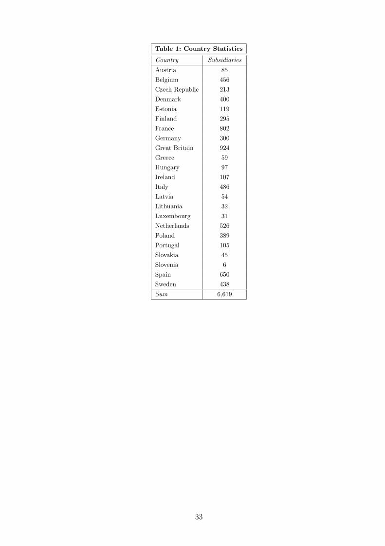
Table 1: Country Statistics

Country Subsidiaries

Austria 85

Belgium 456

Czech Republic 213

Denmark 400

Estonia 119

Finland 295

France 802

Germany 300

Great Britain 924

Greece 59

Hungary 97

Ireland 107

Italy 486

Latvia 54

Lithuania 32

Luxembourg 31

Netherlands 526

Poland 389

Portugal 105

Slovakia 45

Slovenia 6

Spain 650

Sweden 438

Sum 6,619

33

Table 2: Descriptive Statistics

Variable Obs. Mean Median Min. Max.

Subsidiary firms only:

Statutory Corporate Tax RateN 44,739 .3334 .345 .1 .5676

Avg. Tax Difference to All Other AffiliatesH 42,994 -.0071 -.0030 -.3817 .2865

Intangible Fixed AssetsF 44,739 3,303 3 0 1.03e+07

Dummy Intangible Assets� 44,739 .5501 1 0 1

SalesF 37,112 76,107 13,076 1 1.58e+07

Ratio Intangible Assets to Sales 37,112 .022 .0006 0 .9284

Country R&D Expenditures (in % of GDP)I 42,215 1.767 1.833 .3637 4.251

Corruption IndexJ 42,215 7.11 7.10 2.70 10

Population (in million)• 42,215 35.45 39.64 .4336 82.54

GDP per Capita (in thousand Euro)• 42,215 21.93 23.63 2.485 60.31

Growth Rate GDP per Capita (in %)I 42,215 2.391 2.178 -1.496 11.19

Parent firms only:

Intangible Fixed AssetsF 35,554 65,390 583 0 1.98e+07

SalesF 35,554 1,697,070 96,330 1 7.78e+07

Ratio Intangible Assets to Sales 35,554 .0775 .0086 0 3.467

Number of Subsidiaries� 35,554 80.4 29 3 752

Notes: Firm data is exported from the AMADEUS database, TOP-1.5-Million-Version, October 2006.N Obtained from the European Commission (2006) and from KPMG International (2006).H Average Tax Difference to All Other Affiliates calculated as: statutory corporate tax rate of theconsidered subsidiary minus the unweighted average statutory corporate tax rate of all other groupmembers, comprising subsidiaries (owned with at least 90% of the ownership shares) and the parentfirm.F Unconsolidated values, in thousand US dollars, current prices.� Takes on the value 1 if a subsidiary owns intangible assets and 0 otherwise.I Obtained from the World Development Indicators (June 2009) of the World Bank.J From Transparency International (TI), ranks from 0 (extreme level of corruption) to 10 (free ofcorruption).• Taken from the European Statistical Office (Eurostat).� Only subsidiaries owned with ≥ 90% of the ownership shares.

34

Table 3: Baseline Estimations

OLS Firm–Fixed–Effects, Panel 1995–2005

Depend. Variable Log Intangible Assets Log Int./Sales

Explanat. Variables: (1) (2) (3) (4) (5) (6) (7) (8)

Statutory Tax Rate -2.44∗∗∗ -2.38∗∗∗ -2.50∗∗∗ -2.54∗∗∗

(.631) (.663) (.690) (.717)

Av.TaxDiff.toOthers -2.08∗∗∗ -2.01∗∗∗ -2.08∗∗∗ -2.27∗∗∗

(.559) (.584) (.606) (.627)

Log Sales .447∗∗∗ .453∗∗∗

(.026) (.026)

Country R&D Exp. .385∗∗∗ .325∗∗∗ .247∗ .178 .094 .041(.132) (.132) (.140) (.139) (.144) (.143)

Corruption Index .007 -.001 .019 .008 .030 .019(.029) (.029) (.029) (.029) (.030) (.030)

Population .013 .010 -.013 -.020 -.025 -.029(.038) (.039) (.038) (.038) (.038) (.039)

GDP per Capita -.028∗∗ -.028∗∗ -.025∗ -.023 -.021 -.017(.013) (.014) (.015) (.016) (.016) (.016)

Growth GDPp.Cap. .018 .017 -.000 -.003 -.020∗ -.021∗

(.011) (.012) (.011) (.011) (.012) (.012)

Year Dummies√ √ √ √ √ √ √ √

# Observations 44,739 42,994 42,215 40,574 37,112 35,666 37,112 35,666

# Firms 6,619 6,363 6,617 6,361 6,017 5,788 6,017 5,788

Adjusted R2 .7218 .7207 .7274 .7262 .7538 .7531 .7195 .7194

Notes: Heteroscedasticity robust standard errors adjusted for firm clusters in parentheses.∗, ∗∗, ∗∗∗ indicates significance at the 10%, 5%, 1% level. Observational units are multinationalsubsidiaries, i.e. firms that exhibit a foreign parent which owns at least 90% of the ownership shares.Additionally, to be included in the sample, at least one affiliate of the corporate group has to ownintangible assets and at least one has to make positive profits. In (1)–(6), the dependent variable is thenatural logarithm (Log) of the level of intangible assets. In (7)–(8), the dependent variable is the logof the ratio intangible assets to sales (Log (Int./Sales)). In both cases, we add a small constant to theinitial level of intangible assets to avoid losing observations with zero intangibles by taking the log. AnOLS model with fixed firm effects is estimated. Av.TaxDiff.toOthers is defined as the unweighted averagestatutory tax rate difference between the considered subsidiary and all other affiliates of the corporategroup including the parent. Adjusted R2 values are calculated from a dummy variables regressionequivalent to the fixed-effects model.

35

Table 4: Binary Dependent Variable

Logit & OLS Firm–Fixed–Effects, Panel 1995–2005

Dependent Variable: Dummy Intangible Assets

Model Logit Fixed-Effects OLS Fixed-Effects


Statutory Tax Rate -3.36∗∗∗ -4.31∗∗∗ -.271∗∗∗ -.309∗∗∗

(1.14) (1.26) (.102) (.117)

Av.TaxDiff.toOthers -2.71∗∗∗ -2.82∗∗∗ -.218∗∗ -.208∗∗

(1.04) (1.14) (.104)

Log Sales .583∗∗∗ .575∗∗∗ .053∗∗∗ .054∗∗∗

(.048) (.048) (.004) (.004)

Country R&D Exp. .323 .122 .051∗∗ .039(.298) (.298) (.025) (.024)

Corruption Index .085 .047 .006 .004(.067) (.068) (.005) (.005)

Population -.259∗∗∗ -.287∗∗∗ -.016∗∗∗ -.017∗∗∗

(.082) (.083) (.007) (.007)

GDP per Capita -.008 -.015 -.001 -.001(.039) (.038) (.002) (.003)

Growth GDPp.Cap. -.001 -.009 .002 .001(.029) (.029) (.002) (.002)


# Observations 16,734 16,151 13,164 12,726 44,719 42,974 37,102 35,656

# Firms 2,227 2,150 1,884 1,822 6,619 6,363 6,017 5,788

Pseudo or Adj. R2 .0198 .0197 .0596 .0584 .6724 .6709 .6786 .6763

Notes: Heteroscedasticity robust standard errors adjusted for firm clusters in parentheses.∗, ∗∗, ∗∗∗ indicates significance at the 10%, 5%, 1% level. Observational units are multinationalsubsidiaries, i.e. firms that exhibit a foreign parent which owns at least 90% of the ownership shares.Additionally, to be included in the sample, at least one affiliate of the corporate group has to ownintangible assets and at least one has to make positive profits. Dependent variable (Dummy IntangibleAssets) is set to 1 if a subsidiary owns intangible assets and is 0 if not. In (1)–(4), a logit modelwith fixed firm effects is estimated while in (5)–(8) a linear OLS model with fixed firm effectsis applied. Av.TaxDiff.toOthers is defined as the unweighted average statutory tax rate differencebetween the considered subsidiary and all other affiliates of the corporate group including the parent.Adjusted R2 values are calculated from a dummy variables regression equivalent to the fixed-effects model.

36

Table 5: Instrumental Variables Estimations

OLS & IV First–Differences, Panel 1995–2005

Dependent Variable: Log Intangible Assets

Model OLS First Differences IV First Differences


Statutory Tax Rate -1.23∗∗∗ -1.14∗∗∗ -3.15∗∗∗ -3.00∗∗∗

(.419) (.446) (.994) (1.03)

Av.TaxDiff.toOthers -.972∗∗∗ -.961∗∗ -2.31∗∗∗ -2.33∗∗∗

(.390) (.411) (.844) (.880)

Log Sales .318∗∗∗ .320∗∗∗ .333∗∗∗ .337∗∗∗ -.338 -.361 -.233 -.266(.025) (.025) (.027) (.027) (.256) (.265) (.232) (.245)

Country R&D Exp. .109 .090 .472∗∗∗ .421∗∗

(.122) (.124) (.192) (.195)

Corruption Index .019 .010 -.007 -.017(.018) (.018) (.038) (.039)

Population -.021 -.024 -.106∗∗ -.121∗∗∗

(.036) (.036) (.046) (.047)

GDP per Capita -.019∗ -.017 .014 .016(.012) (.012) (.020) (.020)

Growth GDPp.Cap. -.018∗∗∗ -.019∗∗∗ -.012 -.013(.007) (.007) (.016) (.016)


# Observations 32,187 30,917 29,204 28,049 16,424 15,752 15,553 14,912

# Firms 5,709 5,491 5,656 5,439 4,080 3,920 4,048 3,888

1st-stage F-Test of 24.28 22.49 25.35 22.70excl. instr. (F-stat.)

Hansen J-Test .7108 .5267 .5933 .3864(P-value)

Notes: Heteroscedasticity robust standard errors adjusted for firm clusters in parentheses.∗, ∗∗, ∗∗∗ indicates significance at the 10%, 5%, 1% level. Observational units are multinationalsubsidiaries, i.e. firms that exhibit a foreign parent which owns at least 90% of the ownership shares.Additionally, to be included in the sample, at least one affiliate of the corporate group has to ownintangible assets and at least one has to make positive profits. Dependent variable is the naturallogarithm (Log) of the level of intangible assets; we add a small constant to the initial level of intangibleassets to avoid losing observations with zero intangibles by taking the log. In (1)–(4), an OLS model infirst differences is estimated. In (5)–(8), a first-differenced instrumental variables (IV) approach in twostages (2SLS) is applied, with the 1st difference of Log Sales being instrumented with the 2nd–4th lag ofthe level of Log Sales (cf. Anderson and Hsiao, 1982). Av.TaxDiff.toOthers is defined as the unweightedaverage statutory tax rate difference between the considered subsidiary and all other affiliates of thecorporate group including the parent. Note, unobserved time-constant heterogeneity between subsidiariesis controlled for by first-differencing.

37

Table 6: Dynamic Estimations

Difference GMM, Panel 1995–2005

Dependent Variable: Log Intangible Assets

Sample Full Sample No AT,DE,DK


1st Lag Log Int.As. .889∗∗∗ .873∗∗∗ .870∗∗∗ .866∗∗∗ .871∗∗∗ .867∗∗∗ .895∗∗∗ .889∗∗∗

(.036) (.036) (.032) (.033) (.026) (.027) (.029) (.029)

Statutory Tax Rate -1.08∗∗ -1.23∗∗ -1.51∗∗ -1.56∗∗∗

(.547) (.584) (.639) (.626)

Av.TaxDiff.toOthers -1.37∗∗∗ -1.47∗∗∗ -1.38∗∗ -1.18∗∗

(.559) (.581) (.611) (.583)

Log Sales -.031 -.001 -.422∗∗ -.351(.220) (.232) (.210) (.221)

Country R&D Exp. .501∗∗∗ .464∗∗∗ .551∗∗∗ .506∗∗∗ .511∗∗∗ .462∗∗

(.181) (.185) (.195) (.199) (.201) (.204)

Corruption Index -.002 -.007 -.014 -.021 .004 -.004(.031) (.032) (.032) (.033) (.034) (.035)

Population -.122∗∗∗ -.116∗∗∗ -.139∗∗∗ -.142∗∗∗ -.076∗ -.090∗∗

(.035) (.035) (.040) (.041) (.040) (.040)

GDP per Capita .007 .014 .005 .014 .018 .026(.010) (.009) (.014) (.016) (.015) (.016)

Growth GDPp.Cap. .003 .004 .001 .002 .005 .004(.011) (.011) (.012) (.012) (.013) (.013)


# Observations 29,730 28,556 27,950 26,832 24,792 23,792 23,729 22,759

# Firms 5,790 5,570 5,745 5,527 5,128 4,932 4,721 4,535

# Instruments 18 18 23 23 32 32 32 32

Arellano-Bond-Test .213 .180 .222 .194 .342 .327 .364 .366AR(2) (P-value)

Hansen-Test .480 .624 .438 .533 .448 .448 .604 .569(P-value)

Notes: Standard errors robust against heteroscedasticity and autocorrelation within firms are reportedin parentheses. ∗, ∗∗, ∗∗∗ indicates significance at the 10%, 5%, 1% level. Observational units are multi-national subsidiaries, i.e. firms that exhibit a foreign parent which owns at least 90% of the ownershipshares. Additionally, to be included in the sample, at least one affiliate of the corporate group has to ownintangible assets and at least one has to make positive profits. Dependent variable is the natural logarithm(Log) of the level of intangible assets; we add a small constant to the initial level of intangible assetsto avoid losing observations with zero intangibles by taking the log. A one-step linear GMM dynamicpanel-data estimation in first differences is applied. Following Arellano and Bond (1991), we instrumentthe 1st difference of the 1st Lag of Log Intangible Assets with the 2nd and all deeper lags of the levelof Log Intangible Assets. In (5)–(8), we additionally instrument the 1st difference of Log Sales with the2nd and all deeper lags of Log Sales levels. In (7)–(8), subsidiaries located in Austria (AT), Germany(DE) and Denmark (DK) are excluded. Av.TaxDiff.toOthers is defined as the unweighted average statu-tory tax rate difference between the considered subsidiary and all other affiliates of the corporate groupincluding the parent. Note, unobserved time-constant heterogeneity between subsidiaries is controlled forby first-differencing.

38

Table 7: Location of Intangible Assets and Profit Shifting

OLS Firm–Fixed–Effects, Panel 1995–2005

Dependent Variable: Log (Profit before Taxation)

Sample LowIA HighIA IAHighTax IALowTax All Subsidiaries

Explanat. Variables: (1) (2) (3) (4) (5) (6)

Av.TaxDiff.toOthers -2.078∗∗∗ -3.970∗∗∗ -1.958∗∗∗ -3.777∗∗∗ -1.894∗∗∗ 1.327(.445) (.887) (.632) (.744) (.612) (1.800)

Av.TaxDiff.toOthers -1.985∗∗∗

×D.IALowTax (.897)

Av.TaxDiff.toOthers -28.573∗∗

×IntensityDifference (12.530)

Log FixedAssets .017 .088∗∗∗ .075∗∗∗ .008 .047∗∗ .047∗∗

(.021) (.033) (.026) (.033) (.020) (.021)

Log CostEmployees .523∗∗∗ .564∗∗∗ .498∗∗∗ .561∗∗∗ .524∗∗∗ .525∗∗∗

(.048) (.062) (.057) (.065) (.043) (.044)

Country R&D Exp. .279∗∗∗ .396∗ .432∗∗∗ .032 .256∗∗∗ .255∗∗∗

(.110) (.209) (.156) (.160) (.112) (.112)

Corruption Index .056∗∗∗ .074∗ .052∗ .086∗∗ .071∗∗∗ .070∗∗∗

(.024) (.043) (.030) (.036) (.023) (.023)

Population .415∗ .775 .934∗∗ .562 .749∗∗∗ .749∗∗∗

(.287) (.536) (.040) (.424) (.291) (.291)

GDP per Capita .254∗∗∗ .498∗∗∗ .229∗∗∗ .285∗∗∗ .251∗∗∗ .025∗∗∗

(.074) (.147) (.010) (.113) (.074) (.007)

Growth GDPp.Cap. .062∗∗∗ .078∗∗∗ .071∗∗∗ .069∗∗∗ .070∗∗∗ .070∗∗∗

(.012) (.024) (.015) (.020) (.012) (.012)

Year Dummies√ √ √ √ √ √

# Observations 15,034 4,634 7,847 6,348 14,195 14,195

# Firms 3,269 1,079 1,653 1,284 2,937 2,937

Adjusted R2 .7762 .7861 .7604 .7954 .7793 .7790

Notes: Heteroscedasticity robust standard errors adjusted for firm clusters in parentheses.∗, ∗∗, ∗∗∗ indicates significance at the 10%, 5%, 1% level. Observational units are multinationalsubsidiaries, i.e. firms that exhibit a foreign parent which owns at least 90% of the ownership shares.Additionally, to be included in the sample, at least one affiliate of the group has to own intangiblesand at least one has to make profits. Dependent variable is the logarithm (Log) of subsidiary’spre-tax profits. Av.TaxDiff.toOthers is defined as the unweighted average statutory corporate tax ratedifference between the considered subsidiary and all other affiliates of the corporate group includingthe parent. In (1), the sample is restricted to groups which exhibit below average levels of intangibleassets per sales while in (2), the sample is restricted to groups which exhibit above average levelsof intangibles per sales. In (3), the sample is restricted to subsidiaries of MNEs which observe alarger intangible intensity (measured as intangibles over sales) at high-tax affiliates than at low-taxaffiliates while in the contrary, in (4) the sample is restricted to subsidiaries of MNEs which observea larger intangible intensity at low-tax than at high-tax affiliates. In (5)–(6), the full sample of allsubsidiaries is applied. In (5), we interact Av.TaxDiff.toOthers with the dummy D.IALowTax that isset to 1 if the intangible intensity at low-tax affiliates in the group is larger than at high-tax affiliatesin the group, and 0 otherwise. In (6), we interact Av.TaxDiff.toOthers with the variable IntensityD-ifference which captures the difference between the intangibles intensity at low-tax affiliates withinthe group and high-tax affiliates within the group and which is transformed to exhibit only positive values.

39

Documents

Corporate Taxes and the Location of Intangible Assets