Copyright © Cengage Learning. All rights reserved.

4Rational Functions and

Conics

4.2 GRAPHS OF RATIONAL FUNCTIONS

Copyright © Cengage Learning. All rights reserved.

3

• Analyze and sketch graphs of rational functions.

• Sketch graphs of rational functions that have slant asymptotes.

• Use graphs of rational functions to model and solve real-life problems.

What You Should Learn

4

Analyzing Graphs of Rational Functions

5

Analyzing Graphs of Rational Functions

To sketch the graph of a rational function, use the following guidelines.

6

Analyzing Graphs of Rational Functions

You may also want to test for symmetry when graphing rational functions, especially for simple rational functions.

Recall that the graph of f (x) = 1/x is symmetric with respect to the origin.

7

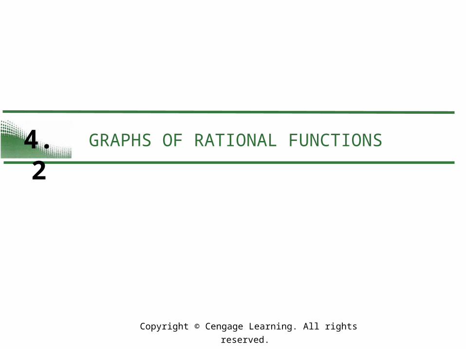
Example 1 – Sketching the Graph of a Rational Function

Sketch the graph of and state its domain.

Solution:

y-intercept: because g(0) =

x-intercept: None, because 3 ≠ 0

Vertical asymptote: x = 2, zero of denominator

Horizontal asymptote: y = 0, because degree of

N(x) < degree of D(x)

8

Example 1 – Solution

Additional points:

By plotting the intercepts,

asymptotes, and a few additional

points, you can obtain the graph

shown in Figure 4.8.

The domain of g is all real numbers

except x = 2.

cont’d

Figure 4.8

9

Analyzing Graphs of Rational Functions

The graph of g in Example 1 is a vertical stretch and a right shift of the graph of because

10

Slant Asymptotes

11

Slant Asymptotes

Consider a rational function whose denominator is of degree 1 or greater.

If the degree of the numerator is exactly one more than the degree of the denominator, the graph of the function has a slant (or oblique) asymptote.

12

Slant Asymptotes

For example, the graph of

has a slant asymptote, as shown in Figure 4.12.

To find the equation of a slant

asymptote, use long division.

Figure 4.12

13

Slant Asymptotes

For instance, by dividing x + 1 into x2 – x, you obtain

As x increases or decreases without bound, the remainder term 2/(x + 1) approaches 0, so the graph of f approaches the line y = x – 2, as shown in Figure 4.12.

Slant asymptote(y = x – 2)

14

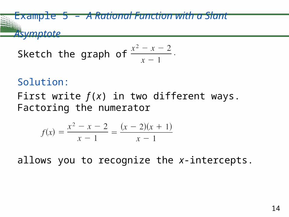
Example 5 – A Rational Function with a Slant Asymptote

Sketch the graph of f (x) =

Solution:

First write f (x) in two different ways. Factoring the numerator

allows you to recognize the x-intercepts.

15

Example 5 – Solution

Long division

allows you to recognize that the line y = x is a slant asymptote of the graph.

y-intercept: (0, 2), because f (0) = 2

x-intercepts: (–1, 0) and (2, 0), because

f (–1) = 0 and f (2) = 0

Vertical asymptote: x = 1, zero of denominator

cont’d

16

Example 5 – Solution

Slant asymptote: y = x

Additional points:

The graph is shown in Figure 4.13.

cont’d

Figure 4.13

17

Application

18

Example 6 – Finding a Minimum Area

A rectangular page is designed to contain 48 square inches

of print. The margins at the top and bottom of the page are

each 1 inch deep. The margins on each side are inches

wide. What should the dimensions of the page be so that

the least amount of paper is used?

19

Example 6 – Solution

Let A be the area to be minimized. From Figure 4.14, you can write

A = (x + 3)(y + 2).

Figure 4.14

20

Example 6 – Solution

The printed area inside the margins is modeled by 48 = xy or y = 48/x. To find the minimum area, rewrite the equation for A in terms of just one variable by substituting 48/x for y.

Use the table feature of a graphing utility to create a table of values for the function

beginning at x = 1.

cont’d

21

Example 6 – Solution

From the table, you can see that the minimum value of y1

occurs when x is somewhere between 8 and 9, as shown in Figure 4.16.

To approximate the minimum value of y1 to one decimal place, change the table so that it starts at x = 8 and increases by 0.1.

cont’d

Figure 4.16

22

Example 6 – Solution

The minimum value of y1 occurs when x ≈ 8.5, as shown in Figure 4.17.

The corresponding value of y is 48/8.5 ≈ 5.6 inches. So, the dimensions should be x + 3 ≈ 11.5 inches by y + 2 ≈ 7.6 inches.

cont’d

Figure 4.17

23

Application

If you go on to take a course in calculus, you will learn an analytic technique for finding the exact value of x that produces a minimum area.

In this case, that value is x = ≈ 8.485.