RATIONAL POINTS ON CONICS

BY

ERIK HILLGARTER

Diplomarbeit

zur Erlangung des akademischen Grades

Diplom-Ingenieur”

n der Studienrichtung

echnische Mathematik

Eingereicht von

Erik Hiligarter

Oktober 7, 1996

Angefertigt amResearch Institute for Symbolic Computation

Technisch-Naturwissenschaftljche FakultätJohannes Kepler Uuiversität

4040 Linz, Austria

Eingereicht beiUniv.-Doz. Dr. Franz Winider

Permission to copy is granted.

.zo~ ui~~qoid/~ido4 ~ ~utpTAo1d aoJ osj~ pu~ s~sa~j~ ~mojdip ~

jo k~tpqissod aq~ ~uuaijo ao,~ 1~pjuiM zu~J~J i~j JOsiAp~ icw o~ ~ UI~ J

SIN~ITNDcI~EIA\ONMOV

ABSTRACT

In order to parametrize an algebraic’ curve of genus zero, one usually faces

the problem of finding rational points on it. This problem can be reduced to find

rational points on a (birationally equivalent) conic. In this paper, we deal with a

method of computing such a rational point on a conic from its defining equation

(we are only interested in exact, i. e. symbolic solutions). The method will then

be extended to work over the rational function field too. This problem arises in

the parametrization of surfaces over Q.

Contents

1 Introduction 3

2 Rational points on rational conics 5

2.1 Problem specification and solution strategy 5

2.2 Simplification of the general conic equation 7

2.2.1 Parabolic case 8

2.2.2 Hyperbolic and elliptic case 11

2.2.3 Algorithm for the parabolic case 15

2.2.4 Algorithm for the hyperbolic/elliptic case . 16

2.3 Solution for the hyperbolic/elliptic case

The Legendre Theorem 19

2.3.1 A proof by Mordell 20

2.3.2 An algorithmic proof 24

2.3.3 An algorithm for solving the Legendre Equation 34

2.4 Real points on rational conics 38

2.4.1 Algorithm for the real case 40

2.5 Concluding Remarks 40

3 Conics over Q(t) 41

3.1 Analogies with the rational case 41

3.1.1 Quadratical residues in Q[t] 48

3.2 Algorithms for Q(t) 50

4 Quadratic forms over arbitrary fields of characteristic ~ 2 58

4.1 Equivalence of quadratic forms 58

4.2 Representation of field elements 61

4.3 Binary quadratic forms 61

A Some numbertheoretic supplements 66

A.1 The Legendre Symbol 66

A.2 A proof of the Legendre Theorem using

Min.kowski’s Lattice Point Theorem 69

B Implementation and Examples 72

B.1 Information for the user 72

B.2 Some examples 76

B.3 The MapleTM code 77

Chapter 1

Introduction

We consider here a subproblem of the so called parametrization problem (see e. g.

[GEBAUER 91], [SENDRA, WINKLER 91], and [SENDRA, WINKLER 96]). The lat

ter consists of computing a parametric representation of an implicitly given (plane) al

gebraic curve of genus zero. In order to tackle that problem algorithmically one faces

the problem of finding rational points on such a curve. This problem can be reduced by

using a theorem of Hilbert/Hurwitz that says that every plane (rational) algebraic curve

of genus zero with degree d ≥ 4 is birationally equivalent to a plane algebraic curve of

genus zero with degree d — 2 (which can be determined algorithmically). Hence, by an

iterated application of the above theorem one will finally face a curve of degree 3 or 2

(depending on whether one started with odd or even degree). Now one can determine

a rational point on this curve and then invert the birational transformations in order to

arrive at a rational point of the original curve. Since every such curve of degree 3 has a

twofold rational singularity, the problem is trivial for curves of odd degree. So the only

remaining problem is to determine a rational point on a plane algebraic curve of degree

2. i.e. on a conic. This is our concerns.

First of all, we show in chapter 2 how to decide whether there is a rational point on

a (rational) conic and - if possible - how to compute such a point. If there is no rational

point on the conic we might content ourselves with determining a real point (which is

a simpler problem). For achieving those goals we transform the defining equation of

the conic to a quadratic form, the so called Legendre Equation, which can be solved by

numbertheoretjc methods.

In chapter 3, I extend this method to the case where the defining conic equation

has rational functions (over Q) as coefficients and the goal is to find a rational function

on this “conic”. This problem arises in the context of parametrizing surfaces over Q.Especially, the following three problems are then solvable

1. Consider a surface F(x,y,t) = 0, where Fe Q[x,y,tJ is of total degree 2 in rand

y. Find a curve on F = 0 that intersects every horizontal plane (i. e. z = coast)

exactly once.

2. Parametrize a conic f(x, y) = 0 (where f e Q(t)[x, y]) with rational functions in s

and coefficients in Q(t).

3. Parametrize a surface F(x, y, t) = 0 (where F ~ Q{x, y, t] is of total degree 2 in x

and y) with rational functions in s and t.

Chapter 4 gives an overview of the (theoretical) situation of quadratic forms over

arbitrary finite fields.

In the appendix the reader finds some numbertheoretic supplements as well as the

Maple code of an implementation together with some examples produced with it.

The potential reader might note that chapter 3 depends heavily on chapter 2. In

order to satisfy the needs of readers who only want to use the results, mathematical

derivations appear in different sections (within a chapter) than algorithms.

Through the whole paper we denote variables by x, y, z (and also primed versions

of them) and we denote rational respectively ir~teger constants by a, b, c, d, e, f (and

primed versions of them).

Chapter 2

Rational points on rational conics

2.1 Problem specification arid solution strategy

In this section, we regard irreducible curves of degree two (so called “conics~) with

rational coefficients, i. e. a conic is defined by an irreducible polynomial g E Q[x, yj of

degree two as the set {(~, ~) E ~2 g(~, ~) = O}. In the sequel we refer to

~ (2.1)

as the general conic equation (2.1). From a geometrical point of view, conics are those

curves that result from cutting a circle cone with a plane. Let us first clarify the problem

under consideration.

Definition 1 (rational point on a conic) We call (~, ~) ~ a rational point on

the conic defined by (2.1) if

g(~) =0.•

By finding a rational point on the conic we understand the following.

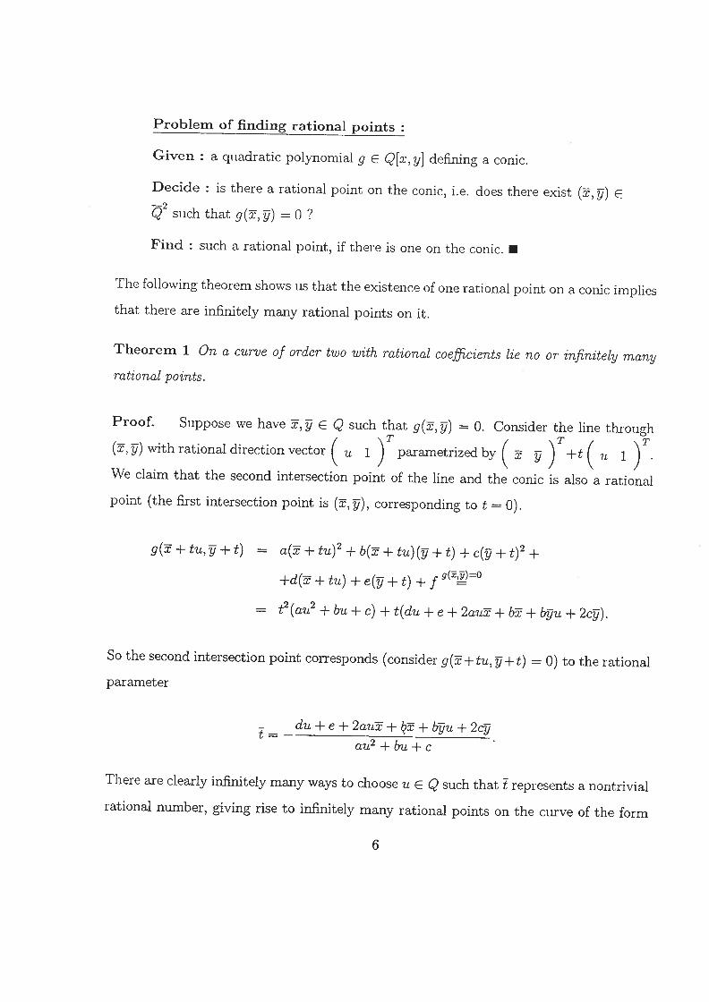
Problem of finding rational points

Given : a quadratic polynomial g ~ Q[x, y] defining a conic.

Decide : is there a rational point on the conic, i.e. does there exist (~, ~) E

such that g(~, ~) = 0?

Find : such a rational point, if there is one on the conic. •

The following theorem shows us that the existence of one rational point on a conic implies

that there are infinitely many rational points on it.

Theorem 1 On a curve of order two with rational coefficients lie no or infinitely many

rational points.

Proof. Suppose we have ~, ~ e Q such that g(~, ~) = 0. Consider the line through

(~, ~) with rational direction vector ( u i parametrized by ( ~ ~ )T+t ( u i )T.

We claim that the second intersection point of the line and the conic is also a rational

point (the first intersection point is (~, ~), corresponding to t 0).

g(~+tu,~-j-t) =

g(~) =0+d(~+tu)+e(~-~-t) +f

= t2(au2+bu+c)+t(du+e+2au~+b~+~u+2~)

So the second intersection point corresponds (consider g(~+ tu, ~+ t) = 0) to the rational

parameter

~au2+bu+c

There are clearly infinitely many ways to choose u E Q such that ~ represents a nontrivial

rational number, giving rise to infinitely many rational points on the curve of the form

6

We will see that it makes sense to distinguish between parabolas on the one hand and

ellipses and hyperbolas on the other hand, since on a parabola, we are guaranteed to

find one (and therefore infinitely many) rational point(s). The principal design of an

algorithm for finding a rational point could be as follows.

ALGORITHM RATIONAL POINT

IN : quadratic polynomial g(x, y) = ax2±b~ry+cy2+dx+ey+f with rational

coefficients.

OUT : Decision of existence of a rational point. A rational point if one exists.

1. Decide if g defines a parabola.

2. If g represents a parabola, compute a rational point on it.

Return “There is a rational point” and return the point.

3. Decide whether g defines an irreducible curve. If not, return “Degenerate case”.

4. Decide whether there is a rational point on the ellipse/hyperbola. If so, compute

one and return “There is a rational point” and return the point.

Otherwise return “No rational point”.

2.2 Simplification of the general conic equation

In order to determine rational points, we will transform (2.1) by an affine change of

coordinates to a more appropriate equation for which solution methods are available. In

this section we give the transformations for the two cases parabola and ellipse/hyperbola

and formulate the corresponding procedures in a PASCAL-like pseudocode.

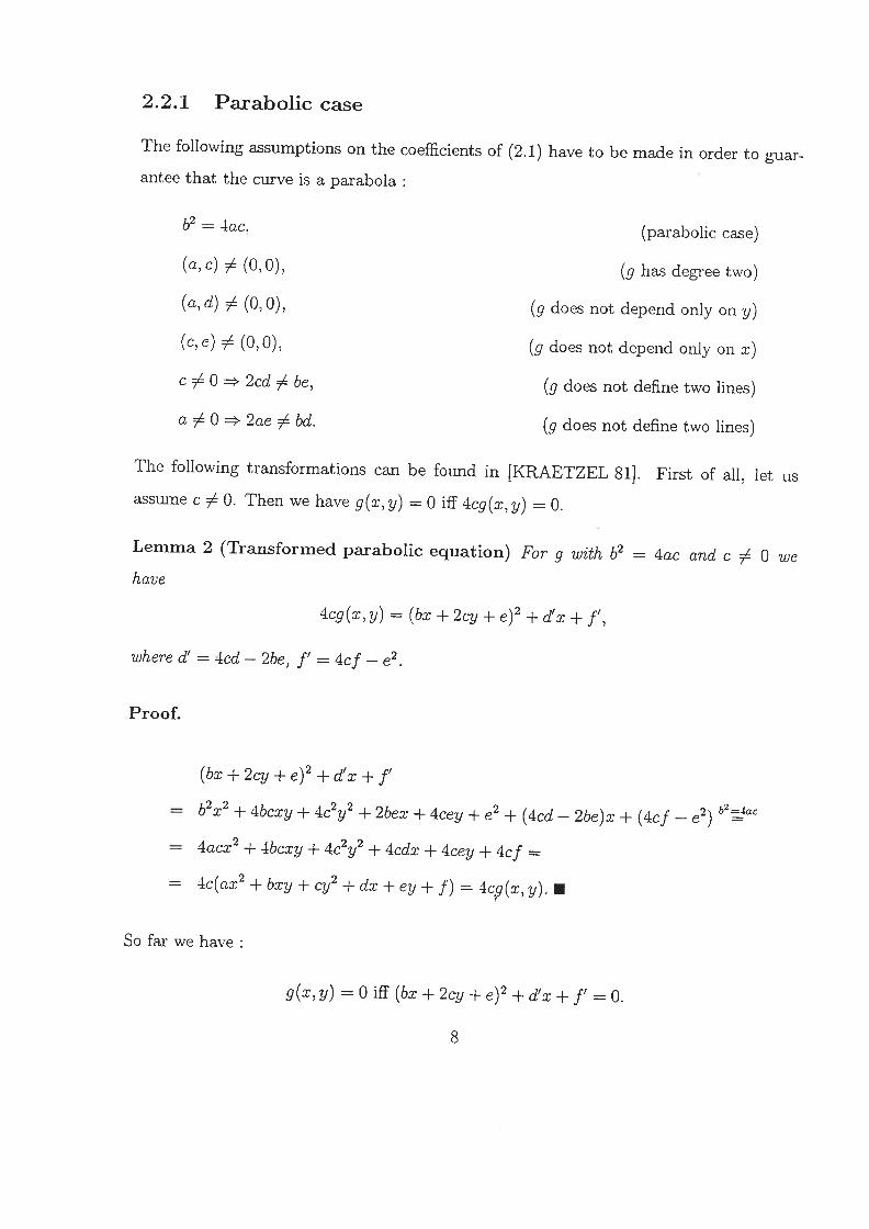
2.2.1 Parabolic case

The following assumptions on the coefficients of (2.1) have to be made in order to guar

antee that the curve is a parabola:

(parabolic case)

(g has degree two)

(g does not depend only on y)

(g does not depend only on x)

(g does not define two lines)

(g does not define two lines)

The following transformations can be found in {KRAETZEL 81]. First of all, let us

assume c ~ 0. Then we have g(x, y) = 0 iff 4cg(x, y) = 0.

Lemma 2 (Transformed parabolic equation) For g with b2 = 4ac and c ~ 0 we

have

4cg(x,y) = (bx+2cy+e)2+d’x+f’,

where d’ = 4cd — 2be, f’ = 4cf — e2.

Proof.

(bx+2cy+e)2+d’x+f’

b2x2 + 4bcxy + 4c2y2 + 2bex + 4cey + e2 + (4cd — 2be)x + (4cf — e2) b2~ac

4acx2 + 1bcxy + 4c2y2 + 4cdx + 4cey + 4cf =

4c(ax2 +bxy+ cy2 +dx+ey+ f) = 4cg(x,y). S

So far we have:

b2 = 4ac

(a,c) ~ (0,0),

(a,d) ~ (0,0),

(c,e) ~ (0,0),

c ~ 0 =~ 2cd ~ be,

a ~ 0 =~ 2ae ~ bd.

g(x,y) = 0 if (bx+2cy+e)2+cfx+f’ =0.

8

At this stage, we might explain why the condition 2cd ~ be (i.e. d’ ~ 0) was required:

(bx + 2cy + e)2 + f’ = 0 is equivalent to bx + 2cy + e = ±~/Ej7. Even if \/E? is not

complex, this equation just defines two parallel (real) lines.

Since we have d’ ~ 0, a rational solution is given by

— f’_ e+b~x = —— y = —_____

d’’ 2c

(One gets this solution by setting the terms inside and outside the brackets to zero

separately).

Now the only remaining case to treat is the one when c = 0. Then - since we required

(a, c) ~ (0,0) - we have a ~ 0. By interchanging the roles of x and y (or by considering

4ag(x, y) = 0 and proceeding as above) we get (be aware of ~ ~—* ~, a ÷—* c, d 4—* e)

d’ = 4ae — 2bcl and f’ = -Iaf — d2. Since d’ ~ 0, a rational solution is given by

f’_ d+b~i2a

EXAMPLES

Example 1 Consider g(x,y) = x2 +y, i.e. (a,b,c,d,e,f) = (1,0,0,0, 1,0).1

Since a ~ 0 we get

d’ = 4ae— 2bd= 4,arid

f’ = 4af — d2 = 0.

So we get

f’ d+by1 0+0y,=—~=O,x,=— 2a 2 0.

(x,,y,) = (0,0) is indeed a solution of g(x,y) = x2 +y = 0.

1 Clearly f 0 implies g(0, 0) = 0.

Example 2 Consider g(x, y) = y2 + x + 1, i.e. (a, b, c, d, e, f) = (0,0, 1, 1,0, 1).

Since c ~ 0 we get

d’ =4cd—2be =4,and

f’ = 4cf — e2 = 4.

So we get

f” e+bx2 0+0X2~l,y2 2c 2 =0.

Indeed, g(—1,0) = 02 + (—1) + 1 = 0.

Example 3 Consider g(x,y) = x2 + 2xy + y2 + x + 2y — 2, i.e. (a,b,c,d,e,f) =

(1,2,1,1,2,—2).

Since a ~ 0 and c ~ 0 we might use both formulae. Let us first of all use the formula for

the case a ~ 0.

d’ = 4ae —2bd= 8—4 —4,and

f’=4af—d2 = —8—1 =—9.

So we get— f’9 — d+&y3 1+~ 11

2a —— 2 ~

Indeed g(—1~, ~) = 0, as one might check.

Now we use the formula for the case c ~ 0 :

d~’ =4cd— 2be = 4—8= —4,arid

f’=4cf—e2 =—8—4=—J2.

Hence we get

12 e+bx4 2+2(—3)x = — — = — — = —3 y = — = — =

d’ 4 ‘ 2c 2

10

Again, g(—3, 2) = 0 holds.

2.2.2 Hyperbolic arid elliptic case

Again we consider (2.1), but we impose other conditions on the coefficients. We use again

[KRAETZEL 81]. First of all, let

D = 4ac — b2,

N = 4de — -lbf,

M1 = 4c2d2 — 4bcde + dace2 + 4b2cf — l6ac2f,

= 4a2e2 — 4bade + 4acd2 + 4b2af — l6ca2f.

With these definitions we require

D~0,

a = c = 0 =~ N ~ 0,

c~40=~M1~40,

a~40=~M2~0,

(c~40AD>O)=~M1 >0,

(a~0AD > 0)=~M2 >0.

(hyperbolic/elliptic case)

(g does not define two lines)

(g does not define two lines)

(g does not define two lines)

(on the conic is more than one real point)

(On the conic is more than one real point)

We consider two cases.

(CASE a = c = 0) In this case we have b ~ 0 and N ~ 0. In the new coordinates

x’ =b(x+y)+d+e,

y’ = b(x—y)—d+e

the equation 4bg(x, y) = 0 has the following form

(x’)2 — (y’)2 = N.

Note that N = 0 would imply that we consider the two lines x’ = y’ and x’ = —y’.

(CASE c ~ 0) We have M1 ~ 0 and (D > 0 =~ ML > 0). Under the coordinate change

= Dx + 2dc — be,

y’ = bx + 2cy + e

the equation 4cDg(x, y) = 0 becomes

(x’)2 + D(y’)2 = M1.

Note that M1 = 0 would imply that we consider the two (possibly complex) lines x’ =

Remark 1 The case a ~ 0 is totally analogous to the case c ~ 0 (just interchange the

roles of x and y and therefore also those of a and c respectively of d and e; in addition

use M2 instead of M1).

Proof. We let MapleTM simplify the considered equations.

(CASE a==c=O)

(b(x+y) +d+e)2— (b(x—y) —d+e)2 — (4de—4bf)

4b

a=c=Oxy+xd+ ye—f = g(x,y).

(CASE c ~ 0)

(x’)2 + D(y’)2 — 1v114cD

=x2a+y2c+f+xd+bxy+yeg(xy).

In both cases we arrived at an equation of the form

+ KY2 = L, (2.2)

where K, L ~ Q, and in both cases we do not have (K> 0 A L < 0), which would exclude

the existence of a real solution.

So let us now consider equations of this form. Switching to homogeneous coordinates

we set

x b’ c’X = ~, Y = ~-, K = —, L =

z z a’ a’

Note that if K = k1/k2, L = 11/12 we may choose a’ = lcm(k2, 12), 1! = k112/ gcd(k2, 12),

and c’ = —11k2/gcd(k2,12). Then (2.2) becomes the Diophantine equation

a’x2 + b’y2 + c’z2 = 0. (2.3)

Clearly a’, b’, and c’ are nonzero and do not all have the same sign (look at their definitions

and use -‘(K > 0 AL > 0)). But we want to achieve more, namely the reduction of (2.3)

to an equation of similar form whose coefficients are squarefree and pairwise relatively

prime. We use ideas from [ROSE 88]. Let us assume that

a’ = al r~, U = U1 r~, c’ = c’~ r~,

where a’1, b’1, and cc are squarefree. Consider

aIx2 + b~y2 + cIz2 = 0. (2.4)

(2.4) has an integral solution if (2.3) has one.. For showing the nontrivial direction,

assume that (2.4) has the integral solution (~, ~, i’). Then

a’ (~-)2+b’ (~)2 (~)2 0,i. e.

13

a’ (~r2 r~ + b’ (~r1 r3)2 + c’ (~rj r2)2 = 0,

giving an integral solution of (2.3).

Remark 2 In the end, we are only interested in the dehomogenization, so the rational

solution (x/r1, ~j/r2, ~/r3) is enough for our purposes.

Now, we divide (2.4) by gcd(a~,b~,c~), getting

a”x2 + b”y2 + c”z2 = 0. (2.5)

What remains is to make the coefficients pairwise relatively prime.

Let g1 = gcd(a”, b”), a” = a”/gj b” = b”/g1, and let (~, ~, ~) be an integral solution of

(2.5). Then 9i I c”~2, and hence, since gcd(a”, b”, c”) = 1, we have g1 ~ Furthermore,

since 9i is squarefree (since a”, b” are), we have g~ ~. So, letting z = g~z’ and cancelling

(2.5) by g1, we arrive at

a”x2 + b”y2+ c”g1 (z’)2 = 0. (2.6)

C.”

We have gcd(a”, U”) = 1 and c” is squarefree since g1 and c” are relatively prime.

Repeating this process with g~ = gcd(a”, c”) and y = g2 y’ we arrive at

“x2+ b”g2 (y’)2 + c”(z’)2 = 0. (2.7)b”

(Again a” = a”/g2, C” =

Now we do it a last time with g3 = gcd(b”, C”) and x = g3 x’. Let a = a”g3, b =

and c = c”/g3. Then we arrive at

a(x’)2 + b(y’)~ + C1~Z’)2 = 0, (2.8)

the so called Legendre Equation. We note : a, b, and c are nonzero, do not all have the

same sign, are squarefree, and pairwise relatively prime. We will treat this equation in

14

section 2.3.

2.2.3 Algorithm for the parabolic case

We use the results gained in subsection 2.2.1 for an algorithmic solution formulated in

pseudocode.

PROC PARABOLA(~g I ok ~ ~ ~

IN:

g e Q[x, yl, g(x, y) = ax2 + bxy + cy2 + dx + ey + f.OUT:

ok : boolean.

(olc = true) if g(x, y) = 0 defines an irreducible parabola.

~ ~je Q.(ok = true) implies g(~, ~) = 0.

LOCAL:

d’, f’ ~ Q.BEGIN

ok := ((a,d) ~ (0,0)) A ((c,e) ~ (0,0)) A (b2 = dac) A ((a,c) ~ (0,0));

if not ok then return;

if (a ~ 0) then

(d’, f’) := (4ae — 2bd, 4af —

if (d’ ~ 0) then

—f’/d’; ~ := —(d + b~)/2a

else

ok := false

end if

else # (c ~ 0)

(d’, f’) := (4cd — 2be, 4cf —

if (d’ ~ 0) then

15

—f’/d’; ~ := —(e + b~)/2c

else

ok := false

end if

end if

END PARABOLA.

2.2.4 Algorithm for the hyperbolic/elliptic case

Here we formulate the knowledge from subsection 2.2.2 in algorithmic form. We assume

the procedures mimer and denom, which deliver numerator and denominator of a rational

number. In addition, sqfrp should deliver the squarefree part of an integer, i.e. for

= fJ p1’-v we havep prime

sqfrp(n) = Jij ~mod(n~2)

p prime

Furthermore, we assume the procedure Legendre (presented in subsection 2.3.3) that

decides whether the Legendre Equation has (nontrivial) integral solutions and eventually

computes one (with z ~ 0). Also the theory of section 2.4 (computing a real point on

the conic in case no rational one exists) is already used here.

PROC~

IN:

a, b, c, d, e, f e Q defining the conic.

OUT:

ok, ratpoint: boolean.

X,YER.

(ok = false) means that we consider either a parabola or two lines, or

that the conic has not more than one real joint.

(ok = ratpoint = true) implies that (X, Y) are coordinates of a

rational point on the conic.

(o/c = true; ratpoirit = false) implies that there is no rational point

on the conic. In this case (X, Y) are coordinates of a real point on the

conic.

LOCAL

D, K, L e Q;ki,k2,l1,12,g,a1,a2,b1, ~,cI,c2,r1r2,r3,gl,g2,g3,x,y,z E Z.

BEGIN

D:=4ac—b2; ok:=D~O;

if not ok then return;

if a=O and c=O then

K:=—1; L:=4(de—bf)

elseif c ~ 0 then

K := D; L := 4c2d2 — 4bcde + 4ace2 + 4b2cf — l6ac2f

else# (a~OAc=O)

K D; L 4a2e2 — 4bade + 4b2af

end if

ok:=L~4OA-~(K>0AL<O);

if not ok then return;

k1 := riumer(K); k2 := denom(K);

numer(L); 12 := denom(L);

g := gcd(k2, 12);

a1 := l2k2/g; b1 := kil2/g; c1 := —11k2/g;

a2 := sqfrp(a1); r1 := sqrt(a1/a2);

sqfrp(b); r2 := sqrt(b1/b2);

C2 := sqfrp(c); r3 := sqrt(c1/c2);

g gcd(a2, b2, c2);

a2 := a2/g; b2 := b2/g; c2 := c2/g;

g1 :=gcd(a2,b2);

a2 := a2/g1; b2 := b2/g1; c2 := c2g1;

g2 :=gcd(a2,c2);

a2 := a2/g2; b2 := b2g2; c2 := c2/g2;

:= gcd(b2, c2);

a2 := a2g3; b2 := b2/g3; c2 c2/g3;

CALL Legendre(~ a2, ~ b2, ~ c2, ~ ratpoirit, T ~ y, ~

if not ratpoint then

if L>Othen

x := sqrt(L); y := 0

else

x =0; y :=

end if

else

x := xg3/r1. y := yg2/r2; z := zgi/r3;

x := x/z; y := y/z

end if

if a = 0 and c = 0 then

X (x-f-y—2e)/2b; Y := (x—y----2d)/2b

elseif c ~ 0 then

X:=(x—2dc+be)/K; Y:=(y—bX—e)/2c

else# (a~OAc=0)

Y := (x — 2ea + bcl)/K; X := (y — bY — d)/2a

end if

END CONIC2

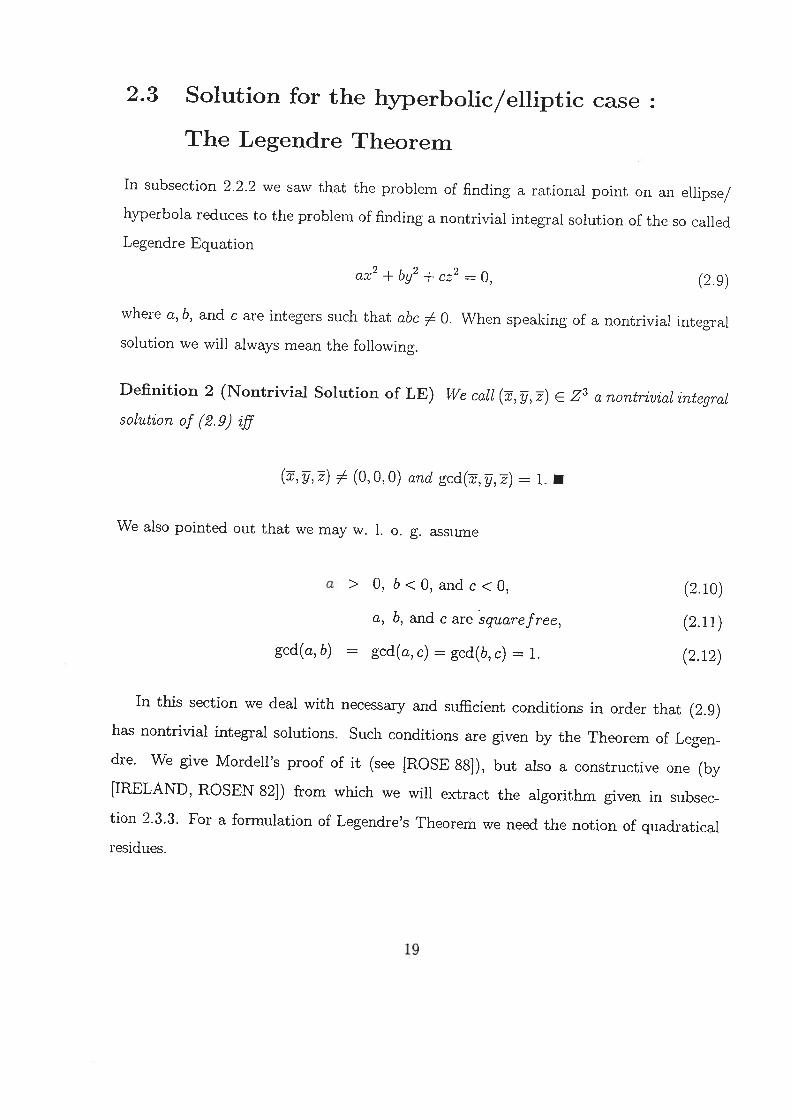
2.3 Solution for the hyperbolic/elliptic case:

The Legendre Theorem

In subsection 2.2.2 we saw that the problem of finding a rational point on an ellipse/

hyperbola reduces to the problem of finding a nontrivial integral solution of the so called

Legendre Equation

ax2 + by2 + cz2 = 0, (2.9)

where a, b, and c are integers such that abc ~ 0. When speaking of a nontrivial integral

solution we will always mean the following.

Definition 2 (Nontrivial Solution of LE) We call (~, ~, ~) E Z3 a nontrivial integral

solution of (2.9) if

~ ~ (0,0,0) and gcd(~,~,~) = 1. S

We also pointed out that we may w. 1. o. g. assume

> 0, b < 0, and c <0, (2.10)

a, b, and c are squarefree, (2.11)

gcd(a,b) gcd(a,c) = gcd(b,c) = 1. (2.12)

In this section we deal with necessary and sufficient conditions in order that (2.9)

has nontrivial integral solutions. Such conditions are given by the Theorem of Legen

die. We give Mordell’s proof of it (see [ROSE 88]), but also a constructive one (by

[IRELAND, ROSEN 82]) from which we will extract the algorithm given in subsec

tion 2.3.3. For a formulation of Legendre’s Theorem we need the notion of quadratical

residues.

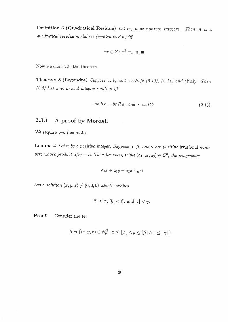
Definition 3 (Quadratical Residue) Let m, n be nonzero integers. Then m is a

quadratical residue modulo n (written m R n) if

~x e Z : rn •

Now we can state the theorem.

Theorem 3 (Legendre) Suppose a. b, and c satisfy (2.10), (2.11) and (2.12). Then

(2.9) has a nontrivial integral solution if

abRc, —bcRa, and — acRb. (2.13)

2.3.1 A proof by Mordell

We require two Lemmata.

Lemma 4 Let n be a positive integer. Suppose a, /3, and 7 are positive irrational num

bers whose product c~4?-y = n. Then for every triple (aj, a2, a3) ~ Z3, the congruence

a1x + a2y + a3z ~ 0

has a solution (~, ~, ~) ~ (0, 0, 0) which satisfies

~ <a, ~ </3, and 1z1 <7.

Proof. Consider the set

S={(x,y,z)eNo3jx<[a]Ay<[/3JAZ<[7j}

20

This set contains (1 + ~aj ) (1 + L/~i) (1+ [~j) > c~37 = n elements. But there are at most

n residue classes modulo n, and so triples (x1, yi, z1) and (x2, Y2, z2) occur in S satisfying

a1x1 + a2y1 + a3z1 ~ a1x2 + a2y2 + a3z2.

The result, follows if we take ~ = x2 — x1, ~ = Y2 — yi, and = z2 — z1. ~

Lemma 5 Let m, n e N with gcd(m, n) = 1. Suppose the form ax2 + by2 + cz2 can be

erpressed as a product of linear factors both modulo m and modulo 7?~. Then it can be

erpressed as a product of linear factors modulo mn.

Proof. Let the conditions be expressed by

ax2 + by2 + cz2 (aix + a2y + a3z)(a4x + a5y + a6z) (mod m),

ax2 + by2 + cz2 (a~x + a~y + a~z)(a~x + a~y + a~z) (mod m).

By the Chinese remainder theorem2 we can find integers a~ satisfying a~ ~m a~ and

a~ ~ a~, for i ~ {1,..., 6}. Combining these congruences we have

ax2 + by2 + cz2 ~mn (a~x + ay + az)(a~x + c4y + a~z). S

Now we proof Legendre’s Theorem.

Proof. (Legendre’s Theorem)

We first show that the conditions (2.13) are necessary. Let (~, ~, ~) be a solution of (2.9);

it follows that gcd(c, ~) = 1. For if any prime p divides gcd(c, ~), then p divides b~2 but

2This theorem states : Let m1, m2,..., m~ be pairwise relatively prime integers > 1, and let Mmlm2...mk. Then there exists a unique nonnegative solution modulo M of the simultaneous congruences

X m1 a1,x —m2 a2, ~X —mk ak. (a~ E Z)

p does not divide b (since gcd(b, c) = 1 by (2.12)) and so p divides ~J. Consequently we

have p2 divides a~2 + b~j2 and hence p2 divides c~’2. But c is squarefree and so p divides

~. This contradicts the assumption gcd(~, ~, ~) = 1.

As gcd(c, ~) = 1 we can find ~‘ satisfying ~‘ ~ 1. Also, clearly

a~2 + ~2 ~ 0,

and so, by multiplying with b(~’)2,

~ —ab(~’)~ ~ —ab.

Thus —ab R c holds. The remaining conditions can be derived similarly.

For proving the reverse implication we deal first with three special cases.

(Case b = c -1) In this case (2.13) gives —1 Ra and so, integers r and s exist sat

isfying r2 + s2 = a (a constructive proof of this fact will be given in section 2.3.2).

Hence in this case (2.9) has the solution~ = (1, r, s).

(Case a = 1, b = -1) Here (2.9) has the solution ~ = (1, 1,0).

(Case a = 1, c = -1) Here (2.9) has the solution ~ = (1,0,1).

In the general case we have —ab R c, that is an integer t can be found to satisfy

~ —ab. (2.14)

Also (since gcd(a, c) = 1 by (2.12)) a* exists satisfying aa* ~ 1. Thus working modulo

c we have

ax2 ~ ~2 ~ cz2 aa* (ax2 + by~) a*(a2x2 + aby2)

a*(a2x2 — ty2) a*(ax — ty)(ax + ty)

(x_a*ty)(ax+ty) (mod c).

22

Using the remaining conditions (2.13) we see that ax2 + by2 + cz2 can also be expressed as

a product of linear factors modulo b and modulo a and so, by Lemma 5, integers a1, ..., a6

can be found to satisfy

ax2 + by2 + C~2 =abc (aix + a2y + a3z)(a4x + a5y + a6z). (2.15)

Note that this holds for all x, y and z. For the next part we consider the congTllence

(aix + a2y + a3z) =abc 0. (2.16)

As we have dealt with three special cases above, and as a, b and c satisfy (2.11) and

(2.12), we may assume that ~ \/E~, and ~/Z~ are irrational. Applying Lemma 4

to (2.16), with ~ = ~, ~ = ~, and ~ = ~. integers x1, y~, and z1 can be found

to satisfy (xi, y~, zi) ~ (0,0,0), a1x1 + a2y1 + a3z1 ~abc 0, and

lxii < ~, y~ <~, and lzii < ~. (2.17)

Now combining (2.15) and (2.17) we have

ax? + by~ + ~ ~ 0.

But, as b and c are negative, (2.17) also gives

ax? + by~ + cz~ ~ ax? <abc, (2.18)

and, as a is positive,

ax? + by~ + cz~ ~ + (2.19)

b(—ac) + c(—ab) = —2abc.

23

These three relations (2.16), (2.18), and (2.19) imply that

ax~+by~+cz~ O,or

ax~ + by~ + cz~ = —abc.

If the first case holds the result follows, so we may assume that the second case holds.

Let

= x1z1 — byj, Y2 = YLZ1 + ax1, z2 = z~ + ab.

This gives

ax~ + by~ + cz~ = a(x1z1 — by~)2 + b(y1zi + axi)2 + c(z~ + ab)2 =

(ax~ + by~ + cz~)z~ — 2abx1y1z1 + 2abx1y1z1 +

+ab(by~ + ax~ + cz~) + abcz~ + a2b2c

= (—abc)z~ + ab(—abc) + abcz~ + a2b2c = 0,

using our assumption. This is a nontrivial solution. For if z~ + ab = 0 then a = 1

and b = —1 as a and b are coprime and squarefree, but this case has been dealt with

previously (see above). Thus nontrivial solutions have been found in all cases and the

proof is complete.

2.3.2 An algorithmic proof

Now we present an algorithmic proof of the Legendre Theorem that gives immediately

an algorithm for finding a solution of (2.9) if one exists (see section 2.3.3). We follow

[IRELAND, ROSEN 82]. First of all let us state the Legendre Theorem again.

24

Theorem 6 (Legendre, Version 1) Let a, b, c be nonzero integers, squarefree, pair-

wise relatively prime and not all positive nor all negative. Then

ax2 + by2 + cz2 = 0 (2.20)

has a nontrivial integral solution if the following conditions are satisfied.

—abRc, (2.21)

—acRb, (2.22)

—bcRa. (2.23)

I

We prove this result in the following equivalent form.

Theorem 7 (Legendre, Version 2) Let a and b be positive squarefree integers. Then

ax2 + by2 = z2 (2.24)

has a nontrivial solution if the following three conditions are satisfied.

aRb, (2.25)

bRa, (2.26)

gcd(a, b)2 R gcd(a, b). (2.27)

Proof. (Equivalence of Theorem 6 and Theorem 7)

(Version 1 implies Version 2) Consider

ax2 + by2 = z2 (2.28)

25

as in Theorem 7. Let g = gcd(a, b), a’ = a/g, b’ = b/g. We know already (compare

subsection 2.2.2) that (2.28) has a nontrivial integral solution if

a’x2 + b’y2 — gz2 = 0 (2.29)

has one. Clearly, a’, b’, and —g are nonzero integers, squarefree, pairwise relatively

prime and, not all positive nor all negative. Hence by Theorem 6, (2.29) has a

nontrivial integral solution if

—a’b’ R — g, (2.30)

—a’(—g) Rb’, (2.31)

—b’(—g) Ra’ (2.32)

are satisfied. (2.30)-(2.32) can be written as

Rg, (2.33)

aRb’, (2.34)

bRa’. (2.35)

But (2.33) already gives (2.27). By (2.34) and aRg we get by Lemma 9 (given

after the proof of Theorem 7) aRb, i. e. we get (2.25). By (2.35) and bRg we get

by Lemma 9 bRa, i. e. we get (2.26).

(Version 2 implies Version 1) We assun~e Theorem 7 and consider (2.20) with a, b,

and c as in Theorem 6. Let us assume that a and b are positive while c is negative.

Then (2.20) has a solution if

—acx2 — bcy2 — z2 = 0 (2.36)

26

has one (compare subsection 2.2.2). But (2.36) satisfies the requirements of Theo

rem 7. So we get

—acR — bc, (by (2.25)) (2.37)

—bcR — ac, (by (2.26)) (2.38)— (—ac)(—bc) Rc. (by (2.27)) (2.39)

Clearly (2.39) gives (2.21), while (2.37) implies (2.22) and (2.38) implies (2.23). ~

Proof. (Theorem 7)

First of all we consider two special (simple) instances of (2.24)

(Case a = 1) Obviously, ~ = (1,0,1) is a solution, and (2.25) - (2.27) hold.

(Case a = b) (2.25) and (2.26) always hold in this case while (2.27) requires —1 to

be a square modulo b. If this is the case, then by Lemma 8 (given immediately

after this proof) we can find integers r and s such that b = r2 + ~2, leading to

a solution ~ = (r,s,r2 + s2). On the other hand, if b(x2 + y2) = z2 has a

nontrivial solution, so has (x2 + y2) = bz2 (compare subsection 2.2.2). Choosing

such a solution (~, ~, ~) gives

X+y6O. (2.40)

Since gcd(~, b) = 1 (remember that we always require gcd(~, ~, ~) = 1), we can

choose ~‘ with ~‘ ~ 1. Multiplying (2.40) by (~f)2 gives

(~~)2 —1,

i. e. —lRb.

Now we proceed to the general case. We may assume a> b, for if b> a just interchange

the roles of x and y. The strategy will be the following : We construct a new form

27

Ax2 + by2 = z2 satisfying the same hypotheses as (2.24), 0 < A < a, and having a

nontrivial solution if (2.24) does so (and a solution of (2.24) can be computed from a

solution of the new form). After a finite number of steps, interchanging A and b in case

A is less than b. we arrive at one of the cases A = 1 or A = b, each of which has been

settled. Now for the details.

We will not reprove the necessity of (2.25) - (2.27) (see the proof of the necessity of

(2.21) - (2.23) in subsection 2.3.1 and the proof of the equivalence of Theorem 6 and

Theorem 7 given above). Therefore we will now assume that (2.25) - (2.27) hold.

By (2.26) there exist integers x and k such that

x2=b+ka. (2.41)

Let k = Am2, where A is the squarefree part of k. Also note that we can choose

such that Ixj ~ a/2 by choosing the absolute least residue of x modulo a (“ symmetric

representation of the integers modulo a”). Let us now restate (2.41) as

= b + Am2a. (2.42)

First of all we show that 0 <A < a. Since

0 ≤ by (~42) b + Am2a sinc~b<a a + Am2a a(1 + Am2)

we have 0 < 1 + Am2, and hence A ≥ 0. But if A = 0, then (2.42) gives x2 = b,

contradicting the fact that b is squarefree. So we established A> 0. On the other hand

2 by (2.42) & b >0 Xl≤a/2 a2Ama < x2 < —

— 4,

and so we have A < Am2 < a/4(< a). So we consider now

Ax2 + bY2 = Z2. (2.43)

28

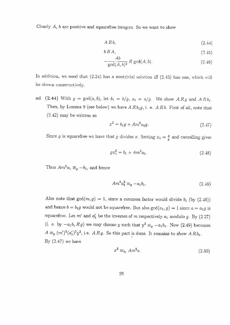
Clearly A, b are positive and squarefree integers. So we want to show

ARb, (2.44)

bRA, (2.45)

gcd(A, 6)2 R gcd(A, b). (2.46)

In addition, we need that (2.24) has a nontrivial solution if (2.43) has one, which will

be shown constructively.

ad (2.44) With g = gcd(a,b), let b1 = b/g, a1 = a/g. We show AR9 and ARb1.

Then, by Lemma 9 (see below) we have A R b1g, i. e. A Rb. First of all, note that

(2.42) may be written as

= b1g + Arn2a1g. (2.17)

Since g is squarefree we have that g divides x. Setting x1 = and cancelling gives

gx~ = b1 + Am2a1. (2.48)

Thus Am2a1 ~ —br, and hence

Am2a~ ~g —a1b1. (2.49)

Also note that gcd(m, g) = 1, since a common factor would divide b1 (by (2.48))

and hence b = b1g would not be squarefree. But also gcd(ai, g) = 1 since a = a1g is

squarefree. Let m’ and a’1 be the inverses of m respectively a1 modulo g. By (2.27)

(i. e. by —a1b1 Rg) we may choose y such that y2 ~g —a1b1. Now (2.49) becomes

A ~Zg (m’)2(a~)2y2, i.e. A Rg. So this part is done. It remains to show A Rb1.

By (2.47) we have

b1 Am2a. (2.50)

29

By (2.25) (i. e. by aRb) we have aRb1. Note also that gcd(a,bj) = 1 since

a common factor would divide b1 and g, contradicting the fact that b = b1g is

squarefree. Similarly, gcd(m, b1) = 1 (use(2.47)). Let a* and rn* be the inverses of

a respectively m modulo b1. Let z be such that z2 ~, a and let z~ be its inverse

rnodulo b1. Now (2.50) becomes

A b1 x2(m*)2a* ~b x2(rn*)2(z*)2,

i. e. ARb1.

ad (2.45) By (2.42), we have bRA immediately.

ad (2.46) With r = gcd(A, b) let A1 = A/r, b2 = b/r. We have to show —A1b2 Rr.

From (2.42) we conclude

= b2r + A1rm2a.

Since r is squarefree we have r divides x. So

A1m2a —b2 (mod r), or

—A1b2m2a b~ (mod r). (2.51)

Since gcd(a, r) = gcd(m, r) = 1, we may choose a+ and m+ as the inverses of a

respectively m modulo r. Furthermore, from (2.25) (i. e. from aRb) we obtain

a Rr. Choose w such that w2 ~r a. Denote by w+ the inverse of w modulo r.

Then (2.51) becomes

—A1b2 ~ b~(m+)2a+ ~,.

i. e. —A1b2 Rr.

30

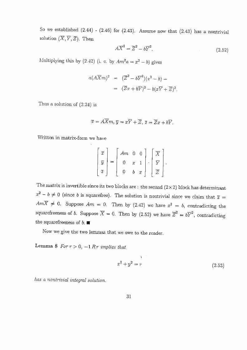
So we established (2.44) - (2.46) for (2.43). Assume now that (2.43) has a nontrivial

solution (X,?, ~). Then

A~2 = — b~2. (2.52)

Multiplying this by (2.42) (i. e. by Am2a = — b) gives

a(A~m)2 (~2 — b~2) (x2 — b) =

= (~x +b~)2 — b(x~+~)2.

Thus a solution of (2.21) is

x=AXm,~=xY+Z~~Zx+by

Written in matrix-form we have

AmOo X

= 0 xl~

0 bx Z

The matrix is invertible since its two blocks are: the second (2 x 2) block has determinant

— b ~ 0 (since b is squarefree). The Solution is nontrivial since we claim that ~ =

AmX ~ 0. Suppose Am = 0. Then by (2.42) we have x2 = b, contradicting the

squarefreeness of b. Suppose X = 0. Then by (2.52) we have Z2 = bY2, contradicting

the squarefreeness of b. ~

Now we give the two lemmas that we owe to the reader.

Lemma 8 For r > 0, —1 Rr implies that

+ ~2 = (2.53)

has a nontrivial integral solution.

Lemma 9 For relatively prime integers nj, n2 we have

aRn1 andaRn2 implies aRn1rz2.

Proof. (Lemma 8)

Since —1 Br, we may choose 10 e N0 and k e N such that x~ = kr — 1, i. e.

+ 1 = kr. (2.54)

Setting Yo 1, we can say that the equation x2 + y2 = kr has the integral solution

(10, Yo). We are done if k = 1. So suppose k> 1. We use the descent method (a common

tool in number theory). We will construct k’ with k’ < k (even k’ ≤ k/2) and 12, Y2 E N0

such that x~ + y~ = k’r. Proceeding inductively, we will finally arrive at a solution of

(2.53).

Let us consider 11 = X~ mod k, and y~ Yo mod ic in symmetric representation of

the integers modulo k. Now we have for some integers c, d

+ y~ = (x~ — ck)2 + (Yo — dk)2 k X~ + ~,g ~ (2.54)

Hence, for some /c’ we have x~ + y~ = k’Ic. Since

x~+y~< (k)~(k)~ ~kk

we have k’ < ~. In addition we have

‘k2r = (k’k)(kr) = (x~ + y~)(x~ + y~) = (101j + yoyi)2 + (x~y1 — xiyo)2.

Dividing by k2 gives

k’r (2021 +Y0Y1)2 + (b0Y1 — XIYo)2

32

So if x2 (x0x1 + yoy1)/k, 1/2 = (x0y1 — xiyo)/k are integers, we have a solution of

x2 + y2 = k’r. But the numerators of x2 (respectively y2) are multiples of k

X0X1 + YoYi = x0(x0 — c/c) + Yo(Yo — dlc) ~zk Xçj + Y~ —k 0,

and

xOy1 — x1y0 x0(y0 — dk) — yo(x0 — ck) ~k O.S

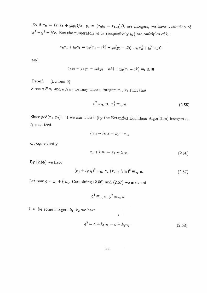
Proof. (Lemma 9)

Since a Rn1 and a Rn1 we may choose integers x1, x2 such that

~ a, ~fl2 a. (2.55)

Since gcd(n1, n2) = 1 we can choose (by the Extended Euclidean Algorithm) integers 1~,

12 such that

11n1 — 12n2 = —

or, equivalently,

X1 + 11n1 = X2 + 12n2. (2.56)

By (2.55) we have

(x1 + ljni)2 ~ a, (x2 + 12n2)2 ~ a. (2.57)

Let now g = x1 + 11n1. Combining (2.56) and (2.57) we arrive at

g2 ~ a, ~2 ~ a,

i. e. for some integers /c1, k2 we have

g2 = a + k~n~ = a + k2n2. (2.58)

33

(2.58) implies k1n1 = k2n2, and hence ri1 divides k2n2. Since ri1, n2 are relatively prime,

n1 divides k2. So, for some integer c we have

k2 = cn1. (2.59)

So, by (2.58) and (2.59) we have

g2 = a + cn1n2,

i. e. we have

a. •

Remark 3 In order to arrive at a rational point on the conic, we need not just any

nontrivial solution (~, ~, ~) but one with ~ ~ 0. In the proof of Theorem 7 an equation

like

— y2 + cz2 = 0

(note a = 1) is equipped with the solution (1, 1,0). Indeed, the existence of a solution

whose z-component is different from 0 is always guaranteed in such a case (see Theorem

19 in section ~ e. g.

~ = (1—c,—1-—c,2).

2.3.3 An algorithm for solving the Legendre Equation

Clearly the constructive proof for the existence of a nontrivial integral solution of (2.20)

in subsection 2.3.2 (under the conditions given there) leads to an recursive algorithm

for computing such a solution. We start with the subproblem considered in Lemma

8, namely the computation of a solution of (2.53). We assume the procedures msqrt

(“modular squareroot”), that has the following meaning: for integers a, b with aRb we

have

msqrt(a, b)2 b a.

34

Such a procedure exists for example in MapleTM. We work in symmetric representation

of the integers modulo any number.

PROC Circle(I r x ~ y)

IN:

r ~ N with —1 Rr.

OUT:

x, y ~ Z such that x2 + ~2 r.

LOCAL

k,x1,y~.h e Z.

BEGIN

x := rnsqrt(—1, r); y := 1; k := (x2 + y2)/r;

while Ic> 1 do

x1 :=xmodk;y1 :=ymodk;

h := (xx1 + yy1)/k; y := (xy1 — xiy)/k;

x := h; k := (x2+y2)/r

end while

END Circle

In the proof of Lemma 8 we saw that Ic drops by a factor of 2 (at least) after each new

assignment to it. The starting value of k can be estimated : x2 + 1 = kr, where lxi ≤ ~.

So we have1 2 1r2 r

k=-(x +1)<-—=-<r.r r4 4

So the number of executions of the while-loop in Circle is bounded by log(r).

In subsection 2.3.2 we saw how to reduce (2.20) to (2.24). This transformation will

be handled by the procedure Legendre. For solving the transformed equation (2.21). it

will call LegendreJ-Jelp, the procedure that does the recursive computation of a nontrivial

integral solution according to the proof of Theorem 7 in subsection 2.3.2. Clearly, Legeri

dre transforms (2.20) and calls LegendreHeip only if a solution exists. So it has to check

the conditions (2.21) - (2.23) of Theorem 6 in subsection 2.3.2. Therefore we assume the

35

procedure £ (“ Legeridre symbol”), which has the following meaning: For integers a, b we

have

L(a,b) = 1 if aRb,

L(a, b) —1 otherwise.

Thus we may test (2.21) - (2.23) in the following way : The conditions are satisfied if

L(—ab, c) + L(—ac, b) + L(—bc, a) = 3.

Also L can be found in MapleTM. Finally we need a procedure sqfrp (“sq’uarefree part”)

for computing the squarefree part of an integer (compare subsection 2.2.4). Now we can

give the pseudocode.

PROC Legenthe(J a ~ b .j. c I solvable ~ x ~ y ~ z)

IN

a, b, c E Z

nonzero, squarefree, pairwise relatively prime, not all positive nor negative.

OUT:

solvable : boolean.

(solvable = true) if ax2 + by2 + cz2 = 0 has nontrivial integral solutions.

x, y, z E Z:

nontrivial integral solution of ax2 + by2 + cz2 0 if solvable = true.

BEGIN

solvable := L(—ab, c) + L(—ac, b) + L(—bc, a) == 3;

if not solvable then return;

if (c <0 and miri(a, b) > 0) or (c> 0 and n~ax(a, b) <0) then

Call £egendreHelp(~ —ac, I —bc, j~ x, ~ y, ~ z);

z := z/c

elseif (a < 0 and min(b, c) > 0) or (a> 0 and max(b, c) <0) then

36

Call LegendreHe1p(~ —ba, 1. —Ca, ~ y, ~ z, ~

x := x/a

else

Call LegendreHe1p(~ —ab, j —cb, ~ y, ~ z, ~

y := y/b

end if

END Legendre

PROC LegendreHe1p(~ a .j. b ~ x T y ~ z)

IN:

a, b e Z:

positive, squarefree with aRb, bRa, —ab/gcd(a, b)2 Rgcd(a, b).

OUT:

x, y, z E Z

such that ax2 + ~2 = z2.

LOCAL

r, s, T, A, B, X, Y, Z, m e Z

BEGIN

if a == 1 then

x := 1; y := 0; z := 1

elseif a == b then

Call Circle(J. b, I x, ~

z := x2 + y2

elseif a> b then

s := m.sqrt(b, a);

T := (s2 — b)/a;

A := sqfrp(T); m := sqrt(T/A);

Call LegendreHelp(~ A, .~ b, ~ X, I Y, ~ Z);

37

x AXm; y := sY + Z; z := sZ + bY

else

s msqrt(a, b);

T := (~2 — a)/b;

A := sqfrp(T); rn := sqrt(T/B):

Call LegendreHelp(~ B, .L a, ~ Y, T X, ~ Z);

y :=BYm; x := sX+Z; z :=sZ+aX

end if

END LegendreHeip

Some words on the number of self-references in LegendreHeip. The worst thing that can

happen is that we reduce both coefficients of

ax2 + by2 =

to 1. The number of self-references of LegendreHeip needed to achieve this is bounded by

2 log4 (max(a, b)), since every time we reduce a coefficient, it is reduced by a factor of 4

at least (see subsection 2.3.2). In the situation a = b we call Circle (and no more call to

LegendreHelp is needed), which calls himself not more than log(a) times (as we know al

ready). So in all cases, the maximal number of any procedure calls is O(log(max(a, b)).

2.4 Real points on rational conies

Let us again consider the general conic equation

g(x,y) = ax~ +bxy+cy2 +~x+ey+f= 0, (2.60)

where a, b, c, d, e, f satisfy the conditions given in subsection 2.2.1 or 2.2.2. Remember

especially that we posed conditions on the coefficients (in the hyperbolic/elliptic case)

38

that guarantee the existence of more than one real point on the conic (e. g. (c ~ 0 A D>

0) =~ M1 ~ 0, see subsection 2.2.2). We do so, because we want to talk here only

about conics whose giaph constitutes something like a realwrv~(so we avoid cases like

x2 + y2 = —1, or x2 + y2 = 0 that would define a purely complex set respectively a set

containing only one real point).3

This time we assume that no rational point lies on the conic. In this case we ask

whether there is at least a real point on the conic, i. e. whether there exists (~, ~) e

such that

= 0.

Under the above assumptions, such a point always exists. Since we saw in subsection

2.2.1 that on every parabola lies a rational point, we only have to consider the ellip

tic/hyperbolic case. In subsection 2.2.2 we transformed (2.60) to an equation of the

form

x2 + Ky2 = L. (2.61)

where K, L are rational numbers satisfying -i(K > 0 A L <0). A real solution of (2.61)

is given by

~ = (‘~/L,0)ifL>o,

(~) = (0,~)ifL<0.

By retransforming, we arrive at a real solution to (2.60).

3Thc question when a rational algebraic plane curve over Q is parametrizable over R is treated insection 3.3 (“Parametrizing over the reals”) of [SENDRA, WINKLER 96]. We state here the main result.

Theorem 10 (Thm. 3.2 of SENDRA, WINKLER 96) A rational algebraic plane curve over Q isparametrizable over R if and only if it is not birationally e.quivalent over R to the conic x2 + y2 + z2.

39

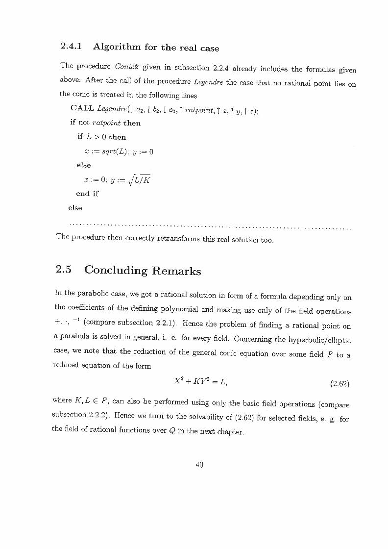
2.4.1 Algorithm for the real case

The procedure Conic2 given in subsection 2.2.4 already includes the formulas given

above: After the call of the procedure Legendre the case that no rational point lies on

the conic is treated in the following lines

CALL Legendre(~ a2, ~ ~ c2, ~ ratpoint, ~ x, T y, I z):

if not ratpoirit then

if L> 0 then

x := sq’rt(L); y := 0

else

x := 0; y :=

end if

else

The procedure then correctly retransforms this real solution too.

2.5 Concluding Remarks

In the parabolic case, we got a rational solution in form of a formula depending only on

the coefficients of the defining polynomial and making use only of the field operations

(compare subsection 2.2.1). Hence the problem of finding a rational point on

a parabola is solved in general, i. e. for every field. Concerning the hyperbolic/elliptic

case, we note that the reduction of the general conic equation over some field F to a

reduced equation of the form

+ KY2 = L, (2.62)

where K, L ~ F, can also be performed using only the basic field operations (compare

subsection 2.2.2). Hence we turn to the solvability of (2.62) for selected fields, e. g. for

the field of rational functions over Q in the next chapter.

40

Chapter 3

Conies over Q(t)

3.1 Analogies with the rational case

As pointed out in section 2.5, we only have to consider the reduced equation

x2 + K(t)Y2 = L(t), (3.1)

where K, L ~ Q(t). Our goal is to find rational functions X(t), Y(t) satisfying (3.1).

This solves the problem of finding rational functions satisfying the general conic equation

with coefficients in Q(t) completely (compare chapter 2). For solving (3.1), we try to

exploit the method used for the rational case. In order to point out the analogy between

these cases, we note that Q(t) is the quotient field of Q[t}, a Euclidean Domain’ (ED for

short), like Q is the quotient field of Z (the standard example of an ED). This means

that we can make use of modular arithmetic, as we did in the rational case. Also those

details of the rational case depending on factorization can be adapted, since every ED is

‘A Eucledian domain is an integral domain J together with a “degree” function d: J~ —* N suchthat

1. Vp,,p~ e : d(p,p2) ≥ d(p,).2. Vp,eJVp~eJ~q,reJ:

Pi =p2q+rA(r~Ovd(r) <d(p2)).In the case J _ Q[tj, d is the usual degree function for polynomials.

a Unique Factorization Domain2 (UFD).

Now let us have a look at the concrete steps performed in the (sub)sections of chapter

2. First of all, we note that we can perform the homogenization of (3.1) as in subsection

2.2.2, leading to an equation of the form

(t)x2 + b(t)y2 + c(t)z2 = 0, (3.2)

where a, b, c e Q{tJ*. Indeed, when we looked at (3.2) over the integers, we also had a sig~i

condition (“a, b, and c do not all have the same sign’~) whose role can be characterized

like this: if it does not hold, then (3.2) has only the trivial solution (at least if we restrict

ourselves to real solutions). The right generalization of this condition at this stage would

be

for every real t0 we have

a(to), b(t0), c(to)

are not all positive, (3.3)

nor all negative.

(Note that this condition would be quite nasty to check). (3.3) is necessary in the

following sense.

Lemma 11 (Necessity of Sign Condition) Suppose (3.3) does not hold. Then the

only polynomial solution of (3.2) is (x(t), y(t), z(t)) (0,0,0).

Proof. (Lemma 11)

Let t0 E R be such that w. 1. 0. g.

a(to), b(to), c(to) > 0.

2A Unique Factorization Domain is a ring R in which every nonzero element a ~ ±1 can be writtenas + the product of primes in at most one way, unique up to the order of the factors.

42

Since polynomial functions are continuous, we might choose 6> 0 such that

for all t e [to — e,t0 +€] we have

a(t), b(t), c(t) are positive.

Now we see that a solution (x(t), y(t), z(t)) of (3.2) has to satisfy

x(t) = y(t) = z(t) = 0 for all t e [to — e, to + e].

But polynomials vanishing on infinitely many points vanish everywhere, i. e.

x(t) y(t) z(t) O.•

Concerning the condition (3.3), we use a simple strategy : we ignore it. Indeed, at a

much later stage, we can easily check whether the order of Q affects the solvability of

(3.2) or not. If one wants to have a (sufficient) criterion that makes it possible to detect

non-solvability at this early stage, then one could test whether lc(a), lc(b), and lc(c) do

all have the same sign; if so then

lim a(t) =lim b(t) =lim c(t) = +00.t—*oo t—+oo t—oc

Hence there exists t0 such that a(to), b(t0), and c(to) do all have the same (nonzero) sign,

and so by lemma 11 equation (3.2) has only the trivial solution. But clearly, this test is

weaker than (3.3).

We are also able to perform the next step of subsection 2.2.2, namely to make a, b, and

c squarefree and (pairwise) relatively prime. The latter is clear since we can compute

the greatest common divisor of polynomials (by the Euclidean algorithm - this holds

for every ED). But also a squarefree factorization of a polynomial can easily be done

(and corresponding commands belong to the kernel of most Computer-Algebra systems).

43

Hence we arrive at an equation of the form

a(t)x2 + b(t)y2 + c(t)z2 = 0, (3.4)

where a. b, c e Q[tl* are sqiiarefree and pairwise relatively prime. Now the three condi

tions given in Legendre’s Theorem Version 1 (Theorem 7, see subsection 2.3.2) for the

rational case

—abRc, (3.5)

—acRb, (3.6)

—bcRa, (3.7)

are also necessary in order that (3.4) is solvable. From now on we assume that we can

decide for two polynomials pi(t), p2(t) whether p~ is a quadratical residue modulo P2

(written Pi Rp2), i. e. whether there exists a polynomial q(t) such that

q(t)2 pj(t) mod p2(t).

So we assume the existence of a function pmsqrt with the property

pi Rp2 implies pmsqrt(p1,p2)2 p~. mod P2.

We will treat a method for computing such a polynomial-modular squareroot at the end

of this section. In addition, we assume the procedure sqfrp (“squarefree part”) and psqrt

(“polynomial squareroot”) that deliver the squarefree part respectively the squareroot of

a polynomial (the latter only if the polynomial is a square).

After having verified that (3.5) - (3.5) hold, we~ can continue the reduction of (3.4) to

a(t)x2 + b(t)y2 = z2 (3.8)

44

as in subsection 2.3.2. Hence a and b are nonzero and squarefree polynomials satisfying

aRb, (3.9)

bRa, (3.10)

gcd(~b)2 Rgcd(a,b). (3.11)

W. 1. o. g. let us assume deg(a) ≥ deg(b). From the proof of Legendre’s Theorem

Version 2 (Theorem 7 in subsection 2.3.2) we know that in the new coordinates

x = AXm,

y = sY+Z,

z = sZ+bY,

where

s(t) = pmsqrt(b(t),a(t)),

s1t~2 b tk(t) = ______

a(t)A(t) = sqfrp(k(t)),

k (t)m(t) = psqrt(~—y),

(3.8) has the form

AX2+bY2=Z2.

In analogy to the rational case A is smaller than a in some sense : in subsection 2.3.3

it was the absolute value of a that dropped; here it is the degree of the polynomial a(t)

that drops.

Lemma 12 Let a(t), b(t) e ~[t}* with deg(a) ≥ deg(b) and deg(a) ≥ 2 such that bRa.

45

Then for

k(t) = s(t)2 where s(t) = pmsqrt(b, a)

we have for some positive integer I

deg(k) = deg(a) — 21, or

deg(k) = 0.

Proof. (Lemma 12)

First of all we note that s(t) can be chosen such that deg(s) ~ deg(a) — 1. Let I E N be

such that

deg(s) = deg(a) —1. (3.12)

Suppose deg(s2) <deg(b). Since

s2(t) = b(t) + k(t)a(t),

we get

deg(s2—b) = deg(k)+deg(a), i. e.

deg(k) = deg(b) — deg(a) ~ 0,

and hence deg(k) = 0 (proving the second case of the lemma). So let us now assume that

deg(s2) ≥ deg(b). (3.13)

Now we have

deg(k) = deg(5 b) = deg(s2 — b) — deg(a) by (3J3)

deg(s2) — deg(a) = 2 deg(s) — deg(a) by (3.12)

46

= 2(deg(a) — 1) — deg(a) = deg(a) — 21. S

Since A(t) = k(t)/m(t)2 we get

2 by Lemma 12deg(A) = deg(k) — deg(m) = deg(a) — 21 — 2deg(m) =

deg(a) — 2n, where ri. = I — deg(m).

Hence the degree of A(t) is smaller than the degree of a(t) by a multiple of 2 (we skipped

here the case deg(k) = 0 which leads to deg(A) = 0, an ideal situation).

Now, by iterated coordinate transformations (as long as the degree of either a or b is

greater than 2), we will finally arrive at one of the following situations

deg(a) = deg(b) = 1, (3.14)

deg(a) = 1, deg(b) = 0 (or vice versa), (3.15)

deg(a) = deg(b) = 0. (3.16)

We will now treat these special cases.

ad (3.14) Since deg(s) ~ deg(a) — 1 we have deg(s) = 0 and hence

— bdeg(k)=deg( a )=deg(b)—deg(a)=0.

This implies deg(A) = 0 and we arrive at (3.15).

ad (3.15)Again deg(s) = 0, i. e. we have

— b = k(t) (a0 + a1t).

a(t)

By comparing degrees on both sides we get k(t) 0, i. e. ~2 = b. Hence a(t)x2 +

b(t)y2 = z2 has the solution (0, 1, .s).

47

ad (3.16) In this case we are confronted with an equation of the form

ax2+&y2=z2, (3.17)

where a, b E Q. Clearly, this case can be treated with the methods of chapter 2.

Remark 4 It is sufficient to search an integral (rational) solution for equation (3.17),

since any polynomial solution implies the existence of many rational solutions by “plug

ging in” (note that this argument works only because a and b do not depend on t I). Also

the question of solvability is only decided at this stage : (3.17) might not have an integral

solution (remember our discussion on the sign-condition for (3.2)). If (3.17) has a non

trivial integral solution, then we invert all coordinate transformations (as in the rational

case), leading to a polynomial solution of (3.2) and finally to a rational function solution

for (3.1) and the general conic equation.

Now we turn to the problem of calculating (at least in principle) the squareroot of a

polynomial modulo another polynomial.

3.1.1 Quadratjcal residues in Q{t]

Suppose we want to determine for two polynomials P1, P2 whether

pi(t) Rp2(t).

We may assume deg(p1) < deg(p2), otherwise we reduce p~ modulo P2• We make an

ansatz q(t) for the polynomial squareroot of p~ modulo P2 of degree deg(p2) — 1. The

polynomial q(t) has to satisfy

q(t)2 pi(t) mod p2(t), i. e.

rem(q(t)2 —p1(t),p2(t)) = 0.

48

This condition gives us equations for determining the unknown coefficients of q(t). The

question whether there are at all any rational solutions for these coefficients decides the

question whether p1(t) Rp2(t) over Q{t]. Let us look at an example.

Example 4 We want to decide whether

t+lRt2

holds, and if it does compute a squareroot of t + 1 modulo t2. We make an ansatz of

degree deg(t2) — 1 (= 1):

q(t) = q0 + q1t.

Now we have

q(t)2 — (t + 1) = q~t2 + (2q0q1 — 1)t + (qg — 1).

Reducing this expression modulo t2 gives

(2q0q1 — 1)t+ (q~ —1).

Equating this remainder to 0 leads to

1,

2q0q1 = 1.

This system has the (rational) solutions (qo, qi) = ±(1, ~). Hence we conclude t + 1 Rt2

and that q(t) = +(~t + 1) is a polynomial squareroot oft + 1 modulo t2. S

From this example we conclude that we deal in general with n polynomial equations

(of degiee 2) in n variables, where n = deg(p2). We might use any of the known tech

niques to solve systems of polynomial equations (Gröbner bases, resultant computation,

characteristic sets, ...). But indeed, this access was quite straight forward and its value

lies more in demonstrating that we can (in principle) decide and compute the discussed

49

items. A more practical access to this problem would be considering a squarefree factor

ization of p~ modulo P2.

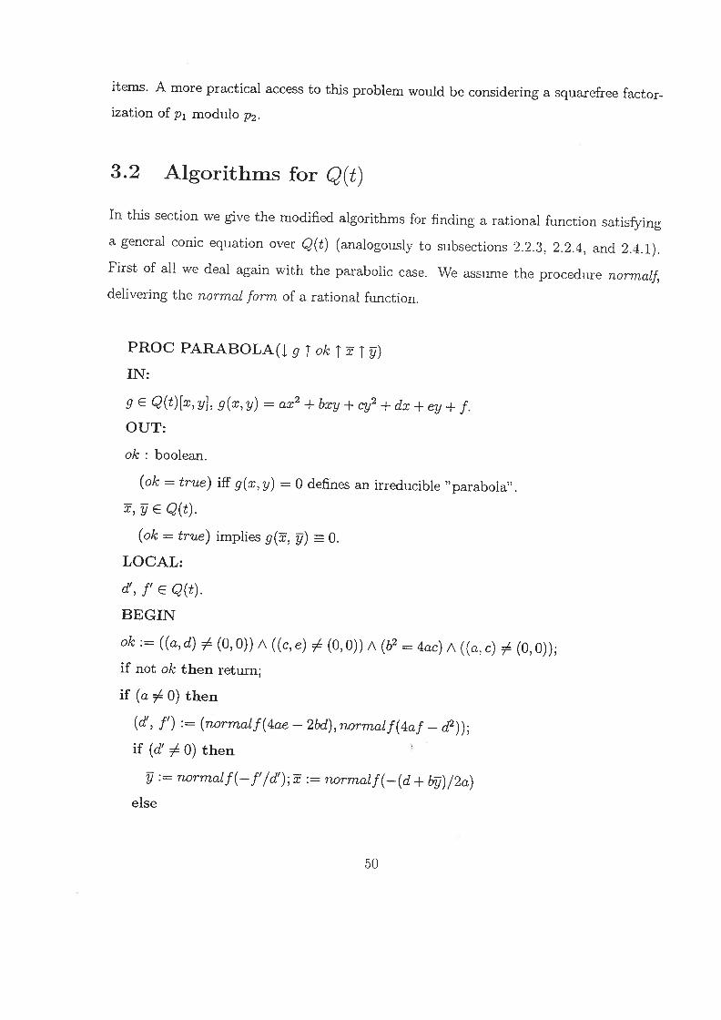
3.2 Algorithms for Q(t)

In this section we give the modified algorithms for finding a rational function satisfying

a general conic equation over Q(t) (analogously to subsections 2.2.3, 2.2.4, and 2.4.1).

First of all we deal again with the parabolic case. We assume the procedure normaif,

delivering the normal form of a rational function.

PROC PARABOLA(J g ~ ok ~ ~ ~

IN:

g e Q(t){x, yJ, g(x, y) = ax2 + bxy + cy2 + dx + ey + f.OUT:

ok : boolean.

(ok = true) if g(x, y) = 0 defines an irreducible “parabola”.

~ Q(t).

(ok = true) implies g(~, ~) 0.

LOCAL:

d’, f’ ~ Q(t).

BEGIN

ok ((a,d) ~ (0,0)) A ((c,e) ~ (0,0)) A (b2 = 4ac) A ((a,c) ~ (0,0));

if not ok then return;

if (a ~ 0) then

(d’, f’) := (normalf(4ae — 2bd), normalf(4af —

if (d’ ~ 0) then

normalf(—f’/d’); ~ := normalf(—(d + b~)/2a)

else

50

ok := false

end if

else # (c ~ 0)

(d’, f’) := (normalf(4cd — 2be), rwrmalf(4cf — e2));

if (d’ ~ 0) then

:= normalf(—f’/d’); ~ := normalf(—(e + b~)/2c)

else

ok false

end if

end if

END PARABOLA.

Now we turn to the analogous algorithm for the procedure conic~ of subsection 2.2.4.

We assume the procedures numer and denom, which deliver numerator and denomi

nator of a rational function. In addition, sqfrp should deliver the squarefree part of a

polynomial, i.e. for p =JJ p~, where the p~ are relatively prime, we have

rrnod(i,2)sqfrp(p) =11 p~

The procedure psqrt should deliver the polynomial squareroot of a polynomial that rep

resents a full square, i. e.

p(t) =.q(t)2 ~ psqrt(p) = q.

The procedure gcd should deliver the greatest common divisor of two (or more) poly

nomials. The procedure lcoeff should deliver the leading coefficient of a polynomial,

while signum delivers the signum of a rational i~umber. Furthermore, we assume the

procedure Legendre (given below) that decides whether the Legendre Equation has (non

trivial) polynomial solutions and eventually computes one (with z ~ 0). Operations like

—, ., / are to be carried out in the field of the (nonzero) rational functions.

51

PROC CONJC2(~a~bTc~dIe~f ok ratpoi t TX TY)

IN:

a, b, c, d, e, f e Q(t) defining the conic.

OUT:

ok, ratpoint: boolean.

X, Y e R(t).

(ok = true) if the general conic equation defines an irreducible

“ellipse” or “hyperbola”.

(ok = ratpoint = true) implies that (X, Y) are rational functions

over ~ on the conic.

(ok = true; ratpoint = false) implies that there is no rational function

on the conic and that (X, Y) = (fail, fail).

LOCAL

D, K, L E

x,y,z E R(t);

k1,k2,l1,l2,g,aj,a2,bl,b2,cjc2rjr2r3g1g2g3~Q[~]

BEGIN

D := normalf(4ac — b2); ok := D ~ 0;

if not ok then return;

if a = 0 and c = 0 then

K —1; L := normalf(4(cte — hf))

elseif c ~ 0 then

K := D; L := normalf(4c2c[2 — 4bcde + 4ace2 + 4b2cf — l6ac2f)

else # (a ~ 0 A c = 0)

K := D; L := normalf(4a2e2 — 4bade + 4b2~zf)

end if

ok := L ~ 0;

52

if not ok then return;

k1 numer(K); Ic2 := denom(K);

numer(L); 12 := denon2(L);

g := gcd(k2, 12);

a1 := normalf(12k2/g); b1 := normalf(k112/g); c1 := normalf(—111c2/g);

olc := —‘(signurn(lcoeff(a)) = signum(lcoeff(b)) = sigrnim(lcoeff(c))):

if not olc then return;

a2 .sqfrp(a1); r1 := psqrt(riorrnalf(aL/a2));

b2 := sqfrp(b); r~ := psqrt(normalf(b1/b2));

C2 := sqfrp(c); r3 := psq’r’t(nor’rnalf(ci/c2));

g := gcd(a2, b2, c2);

a2 := riormalf(a2/g); b2 riormalf(b2/g); c2 := normalf(c2/g);

91 :=gcd(a2,b2);

a2 normalf(a2/g1); b2 := riormalf(b2/g1); c2 := no’rmalf(c2gj);

92 := gcd(a2, c2);

a2 noTmalf(a2/g2); b2 := normalf(b2g2); c2 := normalf(c2/g2);

93 :=gcd(b2,c2);

a2 := normalf(a2g3); b2 := normalf(b2/g3); c2 := normalf(c2/g3);

CALL Legendre(L a2, .~ b2, .L c2, ~ ratpoint, ~ x, ~ y, ~ z);

if ratpoint then

x := normalf(xg3/ri); y := normalf(yg2/r2); z := rioTmalf(zg1/’r3);

x := riormalf(x/z); y := normalf(y/z)

else

if (L E Q) A (K E Q) then

if L>Othen

x := sqrt(L); y := 0

else

x =0; y :=

53

end if

else

X := fail; Y := fail; return

end if

end if

ifa=Oand c=O then

X := riormalf((x + y — 2e)/2b); Y := norrnalf((x — y — 2d)/2b)

elseif c ~ 0 then

X := riormalf((x — 2dc + be)/K); Y := normalf((y — bX — e)/2c)

else# (a#OAc=O)

Y := normalf((x — 2ea + bd)/K); X normalf((y — bY — d)/2a)

end if

END CONIC2

Now we come to the generalizations of the procedures Legendre and LegendreHelp

(compare subsection 2.3.3). We assume the procedure iLSolve that decides and solves

the Legendre equation over the integers. Furthermore we need the boolean function

quadres that decides whether a polynomial is a quadratical residue modulo another

polynomial, i. e. for polynomials a, b E Q[t} we have

quadres(a, b) = true if aRb.

PROC Legendre(j. a .j. b .~ c I solvable ~ x ~ y ‘J~ z)

IN

a, b, c ~ Q{t}

nonzero, squarefree, pairwise relatively prime.

OUT:

solvable : boolean.

(solvable = true) if a(t)x2~i~~b(t)y2-j_c(t)z2 = 0 has nontrivial polynomial solutions.

54

x, y, z e Q[t]

nontrivial polynomial solution of a(t)x2 + b(t)y2 + c(t)z2 = 0 if solvable = true.

BEGIN

if a, b, c E Q then

Call iLSolve(,J. a, .L b, J. c, I solvable, ~ x, ~ y, ~ z);

Return

end if

solvable quadres(—ab, c) A quadres(_ac, b) A quadres(—bc, a);

if not solvable then return;

Call LegendreHelp(~ —ba, .L —ca, ~ solvable, ~ y, ~f’ z, ~

x := x/a

END Legendre

For LegendreHelp we assume pmsqrt, a function that computes the squareroot of a

polynomial modulo another polynomial, i. e. for a, b E Q[tJ with a Rb we have

pmsqrt(a, b)2 a (mod b).

PROC LegendreHelp(J~ a J. b I solvable ~ x ~ y ~ z)

IN

a, b E Q{t}

squarefree polynomials with aRb, bRa, —ab/gcd(a, b)2 Rgcd(a, b).

OUT:

solvable boolean.

(solvable = true) if there exist nonzero polynomials over Q such that

a(t)x2 + b(t)y~ = z2.

x, y, z E Q[tJ

(solvable = true) implies a(t)x2 + b(t)y2 = z2.

LOCAL

55

r, s, T, A, B, X, Y, Z, m E Q{tJ.BEGIN

if degree(a) = 0 and degree(b) = 0 then

Call iLSolve(,J. a, J. b, J. —1, ~ solvable, ~ x, j~ y, ~ z)

elseif degree(a) = 0 and degree(b) odd then

x =1;

y := 0;

z := sqrt(a);

solvable := tr’ue

elseif degree(a) ≥ degree(b) then

s := pmsqrt(b, a);

T normalf((s2 — b)/a);

A := sqfrp(T); m := psqrt(normalf(T/A));

Call LegendreHelp( j. A, ~ b, ~ solvable, ~ X, I )‘~ I Z);

:= normalf(AXm); y := riormalf (sY + Z); z := normalf(sZ + bY)

else

s :=pmsqrt(a,b);

T := rzormalf((s2 — a)/b);

A := sqfrp(T); m := psqrt(normalf(T/B));

Call LegendreHelp(~ B, i a, ~ solvable, ~ ‘f~ X, ~ Z);

y := 7wrmalf(BYm); x := riormalf(sX + Z); z := riormalf(sZ + aX)

end if

END LegendreHeip

Some words on the number of self-references in LegendreHelp. The worst thing that

can happen is that we reduce both coefficients of

a(t)x2 + b(t)y2 = z2

56

~q p~xnpoi si ~i ‘q io v

Jo aai~ap aq~ ~npoi a~ amt~ AJ~A~ a~uis ‘((q)~ap ‘(v)~p)x~ui A~q popimoq S! sn~ ~A~rT{3~

o~ p~p~au d7~Ha.Lpu95~7 jo s~u~iajai-jps jo i~qmnu aqj, ~ ~ai2ap jo sj~ruiou~cjod o~

Chapter 4

Quadratic forms over arbitrary fields

of characteristic ~ 2

In this chapter we describe some of the general properties of quadratic forms over ar

bitrary fields. We shall state some well-known results without proof. Throughout, K

will denote an arbitrary field whose characteristic is not 2. The material is taken from

[BOREVICH, SHAFAREVICH 66].

4.1 Equivalence of quadratic forms

By a quadratic form over the field K we mean a homogeneous polynomial of degree 2

with coefficients in K. Any quadratic form f can be written as (for some n E N)

f = ~i,j=1.

where ~ = ~ ~ K. The symmetric matrix

A =

58

is called the matrix of the quadratic form f. If the matrix is given, the quadratic

form is completely determined (except for the names of the variables). The determinant

d = det(A) is called the determinant of the quadratic form f. If d = 0 the form f is called

singular. and otherwise it is called nonsingular. If we let X denote the column vector

of the variables x1, x2, ..., x~ (and so XT is the row vector of the variables x1, x2, ..., x~).

then the quadratic form can be written as

f = X~AX.

Suppose we replace the variables x1, x2, ..., x,~ by the new variables Yl, y~, ..., y,~ ac

cording to the formula

~ (1≤i<n,c~~éK).

In matrix form this linear substitution becomes

x=cY,

where Y is the column vector of the variables y~, Y2, ..., y~, and C is the matrix

If we replace the variables x1, x2, ..., x,~, in f by the corresponding expressions in yi, Y2, •~.,

then (after carrying out the indicated operations) we shall obtain a quadratic form g (also

over the field K) in the variables y~, Y2, ..., y~. The matrix A1 of the quadratic form g

equals

A1=CTAC. (4.1)

Two quadratic forms are called equivalent, and we write f g, if there is a nonsingular

change of variables which takes one form to the other. From formula (4.1) we obtain the

following theorem.

Theorem 13 If two quadratic forms are equivalent, then their determinants differ by a

59

nonzero factor which is a square in K.

Let y be an element of K. If there exist elements a1, a2, ..., a~, in K for which

f(ai,a2,...,a~) =7,

then we say that the form f represents ~. In other words, a number is represented by a

quadratic form if it is the value of the form for some values of the variables. It is easily

seen that equivalent quadratic forms represent the same elements of the field K.

We shall further say that the form f represents zero in the field K if there exist

values a1, a2, ..., a,, ~ K, not all zero, such that f(a1, a2, ..., a~) = 0. The property of

representing zero is clearly preserved if we pass to an equivalent form.

Theorem 14 If a quadratic form f in n variables represents an element a ~ 0, then it

is equivalent to a form of the type

where g is a quadratic form in n — 1 variables.

Regarding the proof of this theorem we only note the following. If f(a1, a2, ..., a~) =

a, then not all a~ are equal to zero, so we can find a nonsingular matrix C, whose first

row is a1, a2, ..., a,,. If we apply to f the linear substitution whose matrix is C, we obtain

a form in which the coefficient of the square of the first variable is a. The rest of the

proof is carried out as usual.

If the matrix of a quadratic form is diagonal (that is, if the coefficient of every product

of distinct variables equals zero), then we say that the form is diagonal. Theorem 14 now

implies the following theorem.

Theorem 15 Any quadratic form over K can be put in diagonal form by some nonsin

gular linear substitution. In other words, every form is equivalent to a diagonal form.

60

In terms of matrices, Theorem 15 shows that for any symmetric matrix A there exists

a nonsingular matrix C such that the matrix CTAC is diagonal.

4.2 Representation of field elements

Let n be a natural number.

Theorem 16 If a nonsingular form represents zero in the field K, then it also represents

all elements of K.

Proof. Since equivalent forms represent the same field elements, it suffices to prove the

theorem for a diagonal form f = a1x~ + a2x~ + ... +~ Let a1o~ + a2o~ + ... +~ = 0

be a representation of zero, and let -y be any element of K. We can assume that c~ ~ 0.

We express the variables x1, ..., x,~. in terms of a new variable t

x1=c~1(1+t),xk=c~k(1_t) (k=2,...,ri).

Substituting in the form f we obtain

f* f*(t)

0 0~—~--~ -~-~

a1c~(1 + t)2-t- Z a~c~(1 — t)2 = ~ a~c~ +t2 ~ a~c~ +2a1c~t— ~ 2a~c~t =

4a1c~t— ~ 2a~c~t = 4a1~t.

If we now set ~ = -y/4a1a~, we obtain f*(~) =

Theorem 17 A nonsingular quadratic form f represents the element ~ 0 in K if and

only if the form —-y2x~ + f represents zero.

Proof. The necessity of the condition is clear. On the other hand assume that

—7~g+f(~1,...,~~)=O,

where not~ all o~ (i e {O, 1, ..., n}) equal zero. If c~ ~ 0, then y = f(~1/Q’o, ...,

If a0 = 0, then the form f represents zero, and hence by Theorem 16 it represents all

elements of the field K. •

Remark 5 From the proof of Theorem 17 it is clear that if we determine all represen

tations of zero by the form —-yx~ + f (only those in which x0 ~ 0 are relevant,), then we

have also determined all representations of ~ by the form f. Hence the question of the

representability of an element of the field K by a nonsingular form can be reduced to the

question of the representability of zero by a nonsingular form in one more variable.

Theorem 18 If a nonsingular form f represents zero, then it is equivalent to a form of

the following type

YIY2 +g(y3,..,y~).

Proof. Using Theorem 16, we first find c~, ..., c~ such that f(a~, ..., c~) = 1. By

Theorem 14 we can now put f in the form x~ + f1(x2, ..., x~j. Since the form x~ + f~represents zero, we can find /~2, ..., /3~ such that fI(/32, ..., ~3~) = —1. Again applying

Theorem 14, we can put f~ in the form —x~ + g(y3, ..., y,~). Setting x1 — = Yi, and

x1 + x2 = Y2, we obtain the desired result. ~

Remark 6 If we know some representation of zero by the form f, then all the operations

described in the proof of Theorem 18 can be carried out explicitly, and the form g(y3, ..., y1~)

can be determined. Now assume that for any quadratic form which represents zero over

the field K, an actual representation of zero can be found. Then any nonsingular form

can be transformed to a form of the type

(4.2)

62

where the form h does not represent zero. In any representation of zero by the form

~ at least one of the variables Yi, Y2, ~ Y2s—1, Y2s must be nonzero. To determine all

representations of zero in which, say, Yi = c~ ~ 0, we note that we can give 113, •.., y~

arbitrary values a3, ..., a,~ and then determine 1/2 by the condition

This gives us an effective method for finding all representations of zero by a nonsingular

quadratic form over the field K, provided that we have a method for determin

ing whether or not a given form represents zero, and, in case it does, an

algorithm for finding some specific representation of zero.

Theorem 19 Let the field K contain more than five elements. If the diagonal form

a1x~ + ... + a~x~ (a~ ~ K)

represents zero in the field K, then there is a representation of zero in which all the

variables take nonzero values.

Proof. We first show that if aC2 = ~ 0, then for any b ~ 0 there exist nonzero

elements a and ,6 such that aa2 + b/32 = X. To prove this fact we consider the identity

(t—1)2 4t(t + 1)2 + (t + 1)2 =1.

Multiplying this identity by aç~2 = )s~, we obtain

a(Ct 1)2 +at(t~i)2 = ~. (4.3)

Choose a nonzero ~y in K so that the value of t = t0 = b-y2/a is not +1. This can be done

because each of the equations bx2 — a = 0 and bx2 + a = 0 has at most two solutions for

63

x in K, and the field K has more than five elements. Setting t = t0 in (4.3), we obtain

a(~t0 1)2 + b~2~)2 =

and our assertion is proved. We can now easily complete the proof of the theorem. If

the representation a1ç~ + ... + a~ç~ = 0 is such that (i ~ 0, ..., ~ 0, ~ = = 0,

where r ≥ 2, then we have shown that we can find a ~ 0 and ~ ~ 0 such that ar~ =

a,.a2 + ar+j/32, and this yields a representation of zero in which the number of nonzero

variables is increased by one. Repeating this process, we arrive at a representation in

which all the variables have nonzero value. ~

4.3 Binary quadratic forms

A quadratic form in two variables is called binary quadratic form.

Theorem 20 All nonsingular binary quadratic forms which represent zero in K are

equivalent.

Indeed, by Theorem 18, any such form is equivalent to the form YIY2.

Theorem 21 In order that the binary quadratic form f with determinant ci ~ 0 repre

sents zero in K, it is necessary and sufficient that the element —d be a square in K (that

is, —d = a2, a ~ K).

Proof. The necessity of the condition follows from Theorems 13 and 18. Conversely,

if f = ax2 + by2 and —d = —ab a2, then f(a, a) = aa2 + ba2 = —ba2 + ba2 = 0. S

Theorem 22 Let f and g be two nonsingular binary quadratic forms over the field K.

In order that f and g be equivalent, it is necessary and sufficient that their determinants

differ by a factor which is a square in K, and that there exists some nonzero element of

K which is represented by both f and g.

64

c9

.5 f ~Ifl? 15 ‘-~ 1f ~ SU~T~U S1t{~ ~3U~ ‘)J ~ /9’ UaTT~ ‘iop~ ~i~nbs ~

Aq i~~ip ,9’~ pu~ 9’o aDui~ ~fl19’ + ~xo = 15 pu~ ~f~J + ~xo = If suuoj ai~j~ o~ ~u~1~Arnb~

o pu~ f ~j ui~1oaqj, Acj 0 pu~ f q~oq icq po~uos~idoi q~rn~ ~j ~o ~uauiaja

~q o ~ 0 ~J ‘J~3U~13~Jfl9 aAoad O~ A~i~ssooau 4r~p ai~ suoi~ipuo~ q~o~ ~joo.i~

Appendix A

Some numbertheoretic supplements

A.1 The Legendre Symbol

We give some facts (without proof) for the computation of the Legendre Symbol (and

hence on the decision whether a R b for integers a and b) using the law of quadratic

reciprocity. We follow {SCHARLAU, OPOLKA 811.

Let p be an odd prime number and a an integer with gcd(p, a) = 1. Legendre (Adrien

Marie, 1752 - 1833) defined the following symbol’

L(a,p) = 1, if the congruence x2 ~, a is solvable (i. e. if aR p),

L(a,p) = —1, otherwise.

Today, L(a, p) is called the Legendre Symbol. In the first case, a is called a quadratical

residue modulo p, in the second, a quadratical nonresidue modulo p (compare the def

inition in section 2.3). The following theorem provides a first basis for computing the

Legendre Symbol.

1lndeed, Legendre used the symbol(a

for this purpose, but we stay consistent with our notation from chapter 2.

66

Theorem 23 (Law of Quadratic Reciprocity) Letp, q be prime numbers ~ 2. Then

we have

L(p. q)L(q,p) = (_1)~p-1)(q-1) (A.1)

and in addition

L(—1,p) = l,ifp~41,

L(—1,p) = —1, ifp~43. (A.2)

i. e. L(—1,p) = (_i)~(P-1)

Similarly

L(2,p) = 1, ~fP=8 1,7,

L(2,p) = —1, ifp ~ 3,5 , (A.3)

i. e. L(2,p) = (_1)~~2_1).

Formula (A.1,) is called the Law of Quadratic Reciprocity. (A.2) is called the First Sup

plement to the Law of Quadratic Reciprocity. (A.3) is called the Second Supplement to

the Law of Quadratic Reciprocity. •

Remark 7 (A.1) establishes a connection between L(p, q) and L/q,p). Offhand, it is

not immediately clear that these two ez~’pressions are in any way related.

Remark 8 If p is an odd prime number, the multiplicative group F of the field F~ with

p elements is cyclic of order 2. The kernel of the homomorphism )~x.x2 (~ Hom(F~’)) has

order 2. Therefore, (F)2, the image of this homomorphism, has order (p — 1)/2. This

means that F~* contains the same number of squares as nonsquares : [F; : (F~j2} = 2.

(A.1) only deals with primes. We try to generalize the Legendre Symbol L here up

to the point where its arguments can be two odd and relatively prime numbers : Let ~,

67

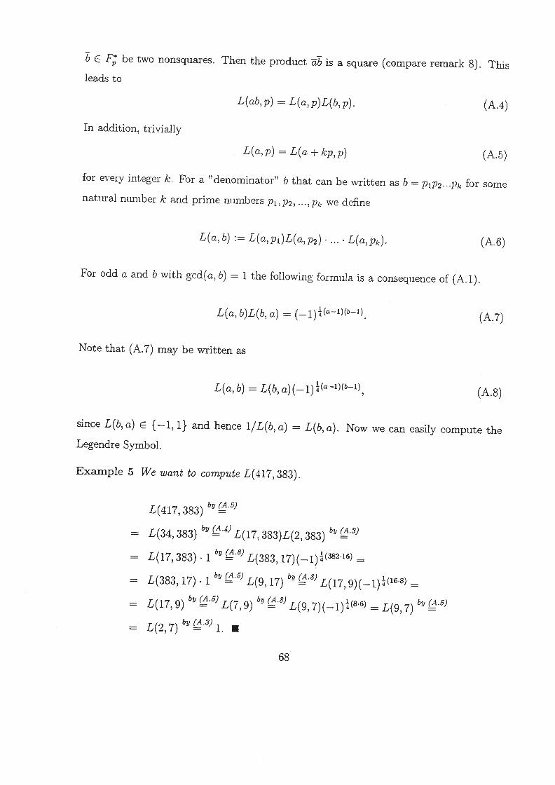
b e F be two nonsquares. Then the product &~ is a square (compare remark 8). This

leads to

L(ab,p) = L(a,p)L(b,p). (A.4)

In addition, trivially

L(a,p) = L(a + kp,p) (A.5)

for every integer k. For a “denominator” b that can be written as b = PIP2• ~~Pk for some

natural number k and prime numbers Pt, P2, ..., Pk we define

L(a,b) := L(a,pi)L(a,p2) ... . L(a,p~.). (A.6)

For odd a and b with gcd(a, b) = 1 the following formula is a consequence of (A.1).

L(a, b)L(b, a) = (_l)~(a_1)(b_1) (A.7)

Note that (A.7) may be written as

L(a, b) = L(b, a)(__1)~(~1)(b_1), (A.8)

since L(b, a) ~ {—1, 1} and hence 1/L(b, a) = L(b, a). Now we can easily compute the

Legendre Symbol.

Example 5 We want to compute L(417, 383).

L(417, 383) by (A.5)

= L(34, 383) by ~ L(17, 383)L(2, 383) by (A3)

L(17,383).1 bY~.B)L(383 17)(_1)~(38216)

L(383, 17). 1 ~v ~ L(9, 17) by ~.8) L(17, 9)(_1)~(168)

L(17, 9) ~ ~ L(7, 9) by ~ L(9, 7)(_1)~(8.6) = L(9, 7) b~ (A.5~

L(2,7) by(~.3) 1. •

68

A.2 A proof of the Legendre Theorem using

Minkowski’s Lattice Point Theorem

In this section we show how Legendre’s Theorem follows of one classical result of number

theory : Mznkowski ‘s Lattice Point Theorem. First of all we state it and give a (sketch

of a) proof. We follow [SCHARLAU, OPOLKA 84].

Theorem 24 (Minkowskj’s Lattice Point Thm.) Let L be a lattice2 in R’~ and K

a centrally symmetric convex set around the origin, i. e., when x, y E K, then —x and

~(x+y) e K. Then, if

vol(K) ≥ 2’~(L),

the set K contains a lattice point x E L, x ~ 0.

Proof. First of all let K be an arbitrary set with a well defined volume, such that

K is disjoint from all the K + x, x e L*. Then we have vol(K) ≤ vol(E), where E is

a fundamental domain. Intuitively, this is obvious; one proves it by decomposing K in

pieces K1, K2, ..., where the pieces lie in different translates of the fundamental domain.

Then one moves the pieces into a fixed fundamental domain where they are disjoint. This

immediately gives our inequality (make a sketch). If vol(K) > ~ i. e., vol(~K) > ~

with ~K = {~xIx e K}, then not all the parallel translates of ~K are disjoint. Therefore

there are ~x,~!y e ~K and z EL, z ~ 0 with ~x = ~y+z or z = ~(x—y). By our

assumption, —y and ~ (x — y) lie in K, which completes the proof. ~

Now let us restate Legendre’s Theorem.

2Let b1 b~ be linear independent column vectors of R’~ (n ≥ 2). Then we call the set

L = {~ akbk : a1, ..., a,~ E Z}

a lattice in R71. The number ~x(L) I det(b1, ..., b,~)j equals the volume of the cuboid spanned by b1, ..., b,.~(the so called fundamental domain) and is called the volume of the lattice.

69

Theorem 25 (Legendre) Let a, b, c be relatively prime square-free integers which do

not all have the same sign. The equation

ax2 + j~2 + cz2 = 0 (A.9)

has a solution (x, y, z) ~ (0, 0, 0) if and only if the following congruences are solvable

—bc (mod a), (A.1O)

v2 —ca (mod b), (A.11)

—ab (mod c). (A.12)

A proof based on Minkowski’s Lattice Point Theorem might run like this.

Proof. The necessity of (A.1O) - (A.12) might be proved as usual (For ax2+by2+cz2 =

0, one has by2 + cz2 0 (mod a) and consequently (cz)2 —bcy2 (mod a). Since we can

assume that x, y, z are relatively prime, y is a unit mod a, consequently x2 —bc (mod a)

is solvable). Conversely, we consider the lattice L of all integral (x, y, z) with

uy cz (mod a),

vz ax (mod b),

wx by (mod c)

for a fixed solution (‘u,v,w) of the congruences (A.10) - (A.12). It is easy to see that

= abcl and that these congruences lead to the congruence

ax2 + by2 + cz2 0 (mod abc), (x, y, z) E L.

We know that the convex centrally symmetrical ellipsoid

K = {(x,y,z) e R3j IaIx2 + bIy2 + cIz2 ≤ R}

has volume 47r/3~R3/~abcJ. According to the Lattice Point Theorem, an element (x, y, z) e(L fl K) with (x, y, z) ~ (0, 0, 0) exists if

> 23Jabc~

or R> (6)2/3IabI

This means that (x, y, z) ~ L with (x, y, z) ~ 0 exists with

Jax2 + by2 + cz2I ≤ ajx2 + Ibjy2 + cjz2 <2IabcI,

i. e., ax2 + by2 + cz2 = 0 or ax2 + by2 + cz2 = ±abc. In the first case, we are finished. If

axg + by~ + cz~ = —abc, then

a(xozo + byo)2 + b(yozo — axo)2 + c(z~ + ab)2 = 0,

and we are finished. To exclude the case ax2 + by2 + cz2 = abc the reader might use the

fact that a, b, c do not all have the same sign. •

Appendix B

Implementation and Examples

In this appendix I describe the MapleTM~irnp1ementecl programs for the user, and we

will see some examples of finding rational points on conics using this implementation. A

section containing the IvIapleTM_code concludes the paper.

B.1 Information for the user

In this section we give an overview of the existing procedures and their function.’

The main procedure (and usually the only procedure a “normal” user will be con

fronted with) is the procedure conic. A usual call has the following form

conic(poly, [x, y},~’ ok” ,“ parabol’,’ ratpoint’,’ X’,’ Y’);

Here poly is the conic equation (a bivariate polynomial of degree 2) with coefficients in Qrespectively Q(t), i. e. poiy is of the form ax2 +bxy+cy2 +dx+ey+f; its indeterminates

are given by the list (here [x, y}) that forms the second argument of conic. conic has 5

output parameters whose role could be characterized as follows:

~Sonietimes we loose some words on how a procedure works; this might not be understood by a readernot familiar with the theory of the previous chapters and hence he should skip such passages.

1. ok : we chose here this name for a boolean variable that checks whether the con

ditions we pose on the general conic equation are satisfied (irreducibility, conic not

purely complex, ...). If so, then ok = true. Otherwise you may ignore the other

output values.

2. parabol the value of this boolean variable equals true iff~ poiy defines a parabola.

3. ratpoirit the value of this boolean variable equals true if there is a rational point

on the conic.

4. (X, Y) : these two rational values satisfy poly(X, Y) = 0 (i. e. constitute a rational

point on the conic) if ratpoirit = true.

In addition to these output parameters, conic returns the value that results from

substituting X and Y into poly as a function value (clearly only in case that there is a

rational point on the conic). This value will always be 0, but this automatic verifying

keeps one from being tempted to “plug in”.

The tasks that conic performs are easily explained : it basically decides whether we

deal with a parabola or an ellipse/hyperbola and deals with these cases by eventually

calling the procedures parabola respectively conic2.

The procedure parabola receives as input values the six coefficients of the general

conic equation and outputs a boolean variable indicating whether we really deal with a

parabola, and if so, the coordinates of a rational point on the parabola. The rational

point is computed by a formula that only depends on the coefficients of the defining

polynomial. A typical call of this procedure looks like this

parabola(a, b, c, d, e, f,’ parabolic’,’ x’,’ y’);

The procedure conic~2 receives as input values the six coefficients of the general conic

equation and outputs two boolean values indicating whether we really deal with an

ellipse/hyperbola and whether there is a rational point on this conic; furthermore it

73

outputs two rational values representing the coordinates of a rational point on the conic

(if one exists; otherwise those output parameters are set to FAIL). A typical call of this

procedure looks like this

conic2(a, b, c, d, e, f,’ ok’,’ ratpoint’.’ X’,’ Y’);

The major task of conic2 is to transform the general conic equation to the corresponding

Legendre equation, call LegeridreSolve for finding an integral (respectively polynomial)

solution of this Diophantine (respectively polynomial) equation, and finally to retrans

form it to a rational solution of the original conic equation.

The procedure LegendreSolve receives as input values the three coefficients of a Legen

dre equation and outputs a boolean value that indicates whether the equation is solvable.

If it is, then the other three output variables contain an integral (respectively polynomial)

solution of the Legendre equation. A typical call of this procedure looks like this

LegendreSolve(a, b, c,’ solvable’,’ x’,’ y’,’ z’);

The procedure decides whether we solve a Diophantine or a polynomial equation and

treats these two cases differently. In the first case the procedure uses iLSolve (a procedure

based on Maples isolve) to solve the Diophantine equation. In the second case the

procedure reduces the Legendre equation to one of a special form (the coefficient of the

third variable is —1) and then uses Legendreffeip in order to get a polynomial solution of

this equation. A retransformation of this solution leads to a polynomial solution of the

original (more general) Legendre equation.

The procedure LegendreHelp receives as input values the two coefficients of a Legendre

equation in special form (the coefficient of the third variable is —1) and outputs a boolean

variable that indicates the solvability of the equation. If the equation is solvable, then

the other three output variables contain a polynomial solution of the Legendre equation.

A typical call of this procedure looks like this

LegendreHelp(a, b,’ solvable’,’ x’,’ y’,’ z’);

The task of LegendreHelp is to recursively transform the given Legendre equation to an

equivalent one, thereby reducing the degrees of the coefficient polynomials. The basic

case of an Legendre equation with rational coefficients is handled again by the procedure

iLSolve.

Other procedures involved are sqfr-p, a function that rehuns the squarefree part of a

polynomial, and quadres, a procedure that decides whether a polynomial is a quadratical

residue modulo another polynomial, and if so, computes the squareroot of this polynomial

rnodulo the other.

75

B.2 Some examples

In this section we give some examples produced with a MapleTM-implementation of the

algorithms given in this paper (whose listing is shown in the next section). First of all

one finds there the three examples carried out by hand in subsection 2.2.1. Then we give

examples of conics that are either not irreducible, purely complex (i. e. do not contain

a real point), or that only contain real points. An example for the non-parabolic case is

taken from [SENDRA, WINKLER 96], section 3.2, namely the conic

— 4xy—3y2 +4x+8y—5 =0.

We try then to give a feeling for the growth2 of the solutions by letting grow the constant

in this polynomial, and finally we also change other coefficients in order to “blow up”

the solution. Five examples with coefficients in Q(t) conclude the section.

We use a short program (the procedure ratpoint) that calls the procedure conic and

handles the output. Also the time needed for the calculation is given (in seconds). The

examples were carried out on a 486 DX / 50 MHz (8 MB RAM).

2~ understand groth here in the rational case in the sense of growing numerators and denominators.

76

> ratpoint := proc(g)> local ok, parab, ratp, X, Y, result, timer;> timer := timeO;> result := conic (g, [x,y] , ‘ok ‘ , ‘parab ‘ ,

> timer := time() - timer;> lprint(’Irreducible conic> iprint ( ‘Parabola> lprint(’Exjstence of a rational point> lprint(’Its x-coordjnates> iprint ( ‘ Its y-coordinates> lprint(’Conic equation evaluated there> lprint(’Time needed for calculation> RETtJRNQ;> end:>> g:=xA2+y: ratpoint(g);

Irreducible conicParabolaExistence of a rational pointIts x—coordjnates

Its y-coordirjates

Conic equation evaluated thereTime needed for calculation

> g:=yA2+x+l: ratpoint(g);Irreducible conicParabolaExistence of a rational pointIts x-coordjnates

Its y-coordinates

Conic equation evaluated thereTime needed for calculation

truetruet rue

>~ratpoint(g);Irreducible conic : trueParabola : trueExistence of a rational point : trueIts x-coordjnates

Conic equation evaluated thereTime needed for calculation

:‘, Ok);:‘, parab);:‘, ratp);:‘); print(X);:‘); print(Y);

, result):‘, timer);

ratp’ ,‘X’ IV!);I -~-

truetruetrue

00

0

0

—1

0

—114

9.’4

00

Its y-coordjnates

00

> g:= x”2 - 2*x*y ÷ 3*yA2 - 2*x - ÷ 3: ratpoint(g);Irreducible conic : trueParabola : falseExistence of a rational point : trueIts x—coordjnates

5Its y—coordinates

3Conic equation evaluated there : 0Time needed for calculation : 3.000

> g:= x~’2 - 2*x*y + 3*y”2 — 2*x - 5*y + 3/2: ratpoint(g);Irreducible conic : trueParabola : falseExistence of a rational point falseIts x—coordjnates

3 r 11~j15 +-~-

Its y—coordinates

1 r— 7~:~J15 ~

Conic equation evaluated there : 0Time needed for calculation : 1.000

> g:= x~’2 + yA2 - 1: ratpo±nt(g);Irreducible conic : trueParabola : falseExistence of a rational point : trueIts x-coordinates

0Its y—coordinates

1Conic equation evaluated there : 0Time needed for calculation : 0

> g:= x”2 + y’2 + 1: ratpoint(g);Irreducible conic : falseParabola : falseExistence of a rational point : failIts x-coordinates

failIts y-coordinates

failConic equation evaluated thereTime needed for calculation : 0

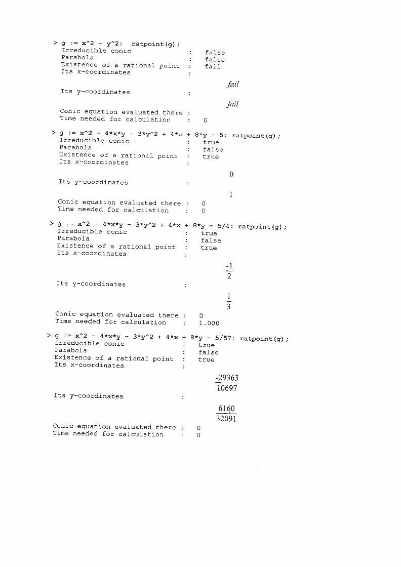
> g := xA2 - yA2: ratpoint(g);Irreducible conic : falseParabola : falseExistence of a rational point failIts x—coordinates

failIts y—coordinates

failConic equation evaluated thereTime needed for calculation : 0

> g := xA2 - 4*x*y - 3*y~’2 + 4*x + - 5: ratpoint(g);Irreducible conic : trueParabola : falseExistence of a rational point : trueIts x—coordinates

0Its y—coordinates

Conic equation evaluated there : 0Time needed for calculation : 0

> g := xA2 — 4*x*y — 3*y”2 + 4*x + - 5/4: ratpoint(g);Irreducible conic : trueParabola : falseExistence of a rational point : trueIts x—coordinates

—12

Its y-coordinates

13

Conic equation evaluated there : 0Time needed for calculation : 1.000

> g := xA2 — 4*x*y — + 4*x + 8*y — 5/57: ratpoint(g);Irreducible conic : trueParabola : falseExistence of a rational point : trueIts x—coordinates

-2936310697

Its y—coordjnates

616032091

Conic equation evaluated there : 0Time needed for calculation : 0

> g : x~2 — 4*x*y - 3*yA2 + 4*x + 8*y - 53/57: ratpoint(g)Irreducible conic : trueParabola : falseExistence of a rational point : trueIts x—coordinates

-829399

Its y—coordinates

128399

Conic equation evaluated there : 0Time needed for calculation : 1.000

> g : xA2 — 4*x*y — 3*yA2 + 4*x + 8*y — 53/589: ratpoint(g)Irreducible conic trueParabola falseExistence of a rational point trueIts x-coordinates

97798934407851283

Its y—coordinates

-50965683407851283

Conic equation evaluated there : 0Time needed for calculation : 1.000

> g := - 4*x*y — 3*yA2 + 4*x + - 540/589: ratpoint(g);Irreducible conic : trueParabola : falseExistence of a rational point : trueIts x-coordinates

74589

Its y—coordinates

32589

Conic equation evaluated there : 0Time needed for calculation : 0

> g := xA2 — — 321/412*y”2 + 4*x + — 540/589: ratpoint(g);Irreducible conic : trueParabola : falseExistence of a rational point : trueIts x—coordinates

-3034547317966475505060385415656351

Its y-coordinates

-19742763146031623215181156246969053

Conic equation evaluated there : 0Time needed for calculation : 0

> g : xA2 — 4*x*y — 32l/412*y”2 + 4*x + 842/523*y — 540/589: ratpoint(g)Irreducible conic : trueParabola : falseExistence of a rational point : trueIts x—coordjnates

-5278101767904785720565977157289164866272537463320158310505421483427

Its y-coordinates

61749401546195669389582248892801324866272537463320158310505421483427

Conic equation evaluated there : 0Time needed for calculation : 2.000

> g := x~2 — 4*x*y — 32l/4l2*yA2 + 428/965*x + 842/523*y — 540/589; ratpoint(g)

2 321 ~ 428 842 540g:=x

Irreducible conic : trueParabola : falseExistence of a rational point : trueIts x—coordjnates

-12261465859644915513874135049501531 14912778572129673865533125424081238782548808348988313982091 0469506000523656433493 98778464

Its y-coordjnates

11 14252096940557370827503010148867541625347355299678747848699703212243716347646425046964941946273 140851800157096930048196335394385

Conic equation evaluated there : 0Time needed for calculation : 27.000

> g := S2/27*X~~2+22/47*X*y_17/39*yA2_61/14*X+4l/l8*y_l7/l3; ratpoint(g);

52 2 22 17 2 61 41 17g:=~x +~Xy-~y -j-4-x+jjy-j-~-

Irreducible conic : trueParabola : falseExistence of a rational point : trueIts x-coordjnates

-4526436000505375613648193523608727824695920668167

Its y—coordinates

15968683599647322519994474607796028693833127027603

Conic equation evaluated there : 0Time needed for calculation : 1.000

> g := _t/(l_t)*xA2 + 2*t*x*y - 2*t*y’~2 - 1*x + 3*y + 2; ratpoint(g);

tx2 2g:=-1 +2txy—2ty —x+3y+2

Irreducible conic trueParabola falseExistence of a rational point trueIts x—coordjnates

-2 -1 + tt

Its y-coordinates

1 4t—3-~.

Conic equation evaluated there : 0Time needed for calculation : 21.000

> g := xA2 - 2*x*y + 4*t/(1_t)*y - 2; ratpoint(g);

2 tyg:~x —2xy+4 —t —2

Irreducible conic : trueParabola : falseExistence of a rational point trueIts x—coordjnates

1 -i + +6 t

-~ -1+tIts y—coordinates

17+t2 + lOt4 -1+t

Conic equation evaluated there : 0Time needed for calculation : 2.000

> g:= t*x’~2 — 2*x*y + (3/t)*y - 2; ratpoint(g);

g tx2 —2 xy + 3 2

Irreducible conic : trueParabola : falseExistence of a rational point trueIts x—coordjnates

1 -3 + 8 t

Its y—coordinates

1

Conic equation evaluated there : 0Time needed for calculation : 0

> g := xA2 - 2*t/(4_t)*x*y + z’2 - 5*t; ratpoint(g);

2 txy 2g:=x ~24_~+z —5t

Irreducible conic trueParabola falseExistence of a rational point trueIts x-coordinates

4Its y—coordjnates

~ (-16 — z2 +5 (-4 + t)

8Conic equation evaluated there 0Time needed for calculation : 4.000

> g := t/(tA2÷3) * zc’~2 2*y + 3; ratpoint(g)

2txg:= 2 -,

t +3

Irreducible conic trueParabola trueExistence of a rational point trueIts x-coordinates

0Its y—coordinates

32

Conic equation evaluated there 0Time needed for calculation 0

B.3 The MapleTM code

This section shows the listing of the implementation used in the previous section. One

~vi11 find two versions. The first one can only handle the case where the coefficients of

the conic equation are in Q. The second version treats the case Q(t), but also handles

the purely rational case correctly (it uses I\Iaples procedure isolve to treat Diophantine

equations). It is this version that produced the examples in the previous section and

that is documented for the user. The first version can be regarded as straight-forward

implementation of the algorithms in chapter 2, and as a basis for the second version.

> parabola := proc(a,b,c,d,e,f,ok,x,y)> local dp, fp, xl, yl;>#># IN:> # a,b,c,d,e,f : fraction.>#># OUT:> # ok : boolean.> # (ok = true) means that> # a*xA2 + b*x*y + c*y’~’2 + d*x + e*y + f = 0 (GCE)> # defines an irreducible parabola.> # x, y : fraction.> # (ok = true) implies that x and y satisfy (GCE)>#># LOCAL:> # dp, fp : fraction.>#>> ok := b”2 = 4*a*c and not (a=0 and c=0) and not (a=0 and d=0)> and not (c=0 and e=0);> if not ok then RETtJRN() fi;>> if f = 0 then x := 0; y := 0; RETURN() fi;> ifa<>Othen> dp := 4*a*e - 2*b*d;> fp := 4*a*f - d”2;> ifdp<>Othen

yl := - fp/dp;> y:=yl;> x : — (d+b*yl)/(2*a)

elseok := false

> fi> else> dp := 4*c*d - 2*b*e;> fp := 4*c*f - eA2;> ifdp<>Qthen> xl := - fp/dp;> x := xl;> y := - (e+b*xl)/(2*c)> else

ok := falsefi

> fi;>

> RETURN()>> end:>

> circle := proc(r,x,y)> local h, k, xl, yl, x2, y2;>#># IN:> # r : integer.> # r has to satisfy : r > 0,> # -1 is a quadratical residue modulo r (written -1 R r).>#># OUT:> # x, y : integer.> # They satisfy x’~2 + y”2 = r. (CE)>#># LOCAL:> # h, k, xl, yl, x2, y2 : integer.>#> ‘mod’ := mods; # symmetric representation> xl := numtheory[imagunit] (r); # now xl”2 = -1 mod r.> yl := 1;> k := (x1’2 + y]/’2) / r;>> whjlek>ldo> x2 := xl modk;> y2 :=ylmodk;> h := (xl*x2 + yl*y2) / k;> yl := (xl*y2 - yl*x2) / k;> xl := h;> k := (xlA2 + ylA2) / r> od;>> x :=xl;> y := yl;>

> RETURN()>> end:>>

> sqfrp := proc(n)> local factorlist, factornumber, signu, factorof, exponent, result, i;>#># IN:> # fl : integer;>#># OUT:> # the squarefree part of n as function value.>#># LOCAL:> # factorljst : list.> # factornuinber, factorof, signu, exponent, result, i : integer.>#> if n = 0 then RETUPN(1) fi;> readlib(isqrfree);> factorlist := isqrfree(n);> # Now factorljst = [ sign(n), [[f(l),e(1)J,...,[f(m)e(m))J ],> # where n = sign(n)*f(1)Ae(1)* . *f(~~ is a squarefree> # factorization of n.> # The squarefree part of n can then be expressed as> # sign(n)*f(~)A(~(~) mod 2)*. . .*f(m)’~(e(m) mod 2).>> factornumber := nops(factorlist[2]);> result := 1;> signu := factorlist[1];>> for i to factornuinber do> factorof := factorlist[2][i][1];> exponent := factorlist[2] [i] [2];> result := result * factorofA (exponent mod 2)> od;>> result := result * signu;>> end:>>

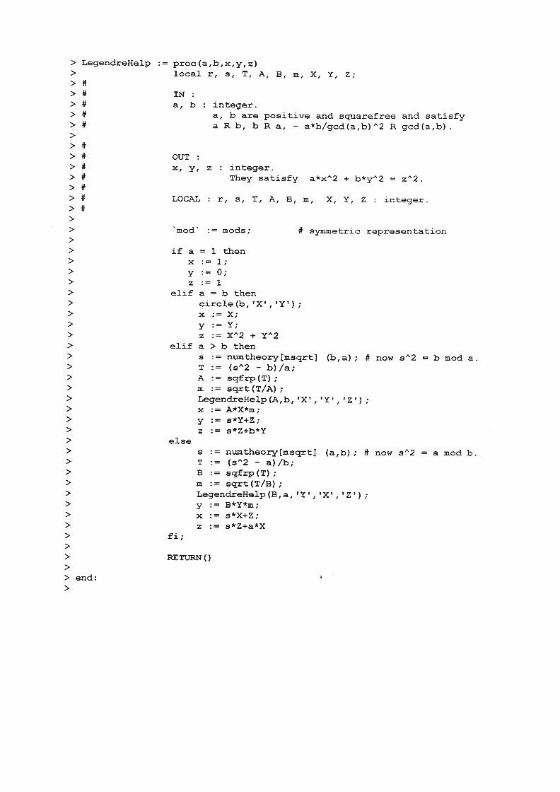
> Legend.reHelp : = proc (a ,b , x, y, z)> local r, s, T, A, B, m, X, Y, Z;>#># IN:> # a, b : integer.> # a, b are positive and squarefree and satisfy> # a R b, b R a, - a*b/gcd(a,b)”2 R gcd(a,b).>>#># OUT:> # x, y, z : integer.> # They satisfy a*x~’2 + b*yA2 = z’~2.>#> # LOCAL : r, s, T, A, B, m, X, Y, Z : integer.>#>> ‘mod~ : = mods ; # symmetric representation>> ifa=1 then> x:=l;> y:=O;> z:=l> elifa=bthen> circle(b, ‘X’, ‘Y’);> x:=X;> y:=Y;> z :=XA2+Y~2> elifa>bthen> s := numtheory[msqrt) (b,a); # now = b mod a.> T := (s’2 —

> A := sqfrp(T);> m := sqrt(T/A);> LegendreHelp(A,b, tX’, ‘Y’, ‘Z’);> x : A*X*m;> y := s*Y+Z;> z := s*Z+b*y> else> s := numtheory[msqrt) (a,b); # now = a mod b.> T := (5A2 — a)/b;> B := sqfrp(T);> m : sqrt(T/B);> LegendreHelp(B, a, ‘Y’, ‘X’, ‘Z’);> y := B*Y*m;> x := s*X+Z;> z := s*Z+a*X> fi;>

> RETtJRN()>>end:>

> Legend.resojve : = proc (a,b, c, solvable ,x,y, z)> local X, Y, Z;>#># IN:> # a, b, c : integer.> # a, b, c are nonzero, squarefree, pairwise> # relatively prime and not all positive nor> # all negative.>#># OUT:> # solvable : boolean.> # x, y, z : integer.> # (solvable = true) implies that> # a*xA2 + b*y~’2 + c*zA2 = 0 (LE)> # has a nontrivial integer solution.> # If so, then (x,y,z) is one with z <> 0.>#># LOCAL:> # X, Y, Z : integer.>#> solvable

evalb(numtheo~[L](_a*b,ab$(c)) +> numtheory[LJ (_a*c,abs(b)) +

> numtheory[L)(_b*c,abs(a)) =3);

if not solvable then RETtJRN() fi;>#> # The first “if” avoids z 0.>#> if abs(a) = 1 and abs(b) = 1 and a <> b then>> if abs(c) = 1 then> if a = c then # Case +- (x”2 - y”2 ÷ z”2) = 0.

x :=0; y :=1; z :=l> else # Case +~ (xA2 — y~’2 — zA2) = 0.> X:=l;y:0;z :=1> fi> else> if a = 1 then # Case +- (x”2 - yA2 + c*z”2) = 0.

x := 1-c; y := -1-c; z : 2> else # Case +— (_xA2 + yA2 + c*zA2) = 0.> x := -1-c; y := 1-c; z =2> fi> fi;

> RETURN()> fi;>> if (c < 0 and min(a,b) > 0) or (c > 0 and max(a,b) < 0) then> LegendreHelp(_a*c,_~*~, 1x~, ‘y’, ‘Z’) ;> z :=Z/c> elif (a < 0 and min(b,c) >0) or (a > 0 and max(b,c) <0) then> LegendreHelp(_a*~,_~*~, ‘y’, ‘z’, ‘X’)> x:=X/a> else> LegendreHelp (—a*b, _b*c, ‘x’, ‘z’, ‘Y’)> y:=Y/b> fi;>

> RETURN()>> end:>

> conic2 := proc(a,b,c,d,e,f,okratpojntXy)> local D, K, L, ki, k2, 11, 12, g, al, a2, bi, b2, ci, c2,> ri, r2, r3, gi, g2, g3, x, y, yl, z, ratp, oki;>#># IN:># a, b, c, d, e, f : rational.> # They define a conic via> # g(x,y) = a*xA2 + b*x*y + c*yA2 + d*x + e*y + f = 0. (GCE)>#># OUT:> # ok, ratpoint : boolean.> # X, Y : real.> # (ok = true) implies that (GCE) defines an> # irreducible ellipse or hyperbola with at least> # two real points.> # (ok = ratpoirit = true) implies that (X,Y) are> # rational coorthnates of a point on the conic.> # (ok = true; ratpoint = false) implies that (X,Y) are> # real coordinates of a point on the conic and that> # no rational point lies on the conic.>#># LOCAL:> # D, K, L : rational.># x, y, z : real.># ~> # gi, g2, g3 : integer.> # ratp, okl : boolean.>#> D := 4*a*c — bA2;> oki := evalb(D <> 0);> if not oki then ok := oki; PETt.TRN() fi;>#> # Transformation of (GCE) in dependence of the values of a and c.>#> ifa=OandcOthen>> L := 4*d*e - 4*b*f> elif c <> 0 then>> L := 4*0A2*dA2 — 4*b*c*d*e + 4*a*c*eA2 + 4*bA2*c*f — l6*a*c’~2*f> else # if a<>0 and c=0>> L := 4*aA2*eA2 — 4*b*a*d*e + 4*bA2*a*f -

> fi;>#> # Now (CCE) is equivalent to> # xA2 + K*y”2 = L. (TE)>#

> oki L <> 0 and not(K > 0 and L<0); # degenerate cases> ok := oki;> if not oki then RETURN() fi;> # Some very special case> if f = 0 then ratpoint := true; X 0; Y := 0; RETURN() fi;>> ki := numer(K); k2 := denoxn(K);> 11 numer(L); 12 denom(L);> g := gcd(k2,12);> al := l2*k2 / g; bi := ki*12 / g; ci := — l1*k2 / g;>#> # Now (TE) is equivalent to the diophantine equation> # ai*xA2 + b1*y~2 + cl*zA2 = 0. (DE)>#> a2 := sqfrp(ai) ; ri := sqrt(al/a2)> b2 := sqfrp(bi) ; r2 := sqrt(bi/b2)> c2 := sqfrp(ci) ; r3 := sqrt(ci/c2)> g gcd(a2 ,gcd(b2,c2));> a2 := a2/g; b2 := b2/g; c2 := c2/g;> gi := gcd(a2,b2);> a2 := a2/gi; b2 b2/gl; c2 := c2*gl;> g2 :=gcd(a2,c2);> a2 := a2/g2; b2 := b2*g2; c2 c2/g2;> g3 := gcd(b2,c2);> a2 a2*g3; b2 := b2/g3; c2 :=c2/g3;>#> # Here, (DE) is equivalent to> # a2*(xI)~2 + b2*(yI)’~2 + c2*(z1)’~2 = 0,> # where x’ = x * ri / g3, y’ = y * r2 / g2, z’ = z * r3 / gi.> # In addition, a2, b2, c2 satisfy the input-requirements> # of LegendreSolve.>#> Legendresolve (a2 ,b2 ,c2, ‘ratp’, ‘x’, ‘y’, ‘z’)> ratpoint ratp;> if ratp then # we arrive at a rational solution for (TE).> x :=x * g3 / ri; y :=y * g2 / r2; z z * gi / r3;>> x:=x/z;y:=y/z> else # we only arrive at a real solution for (TE)> ifL>Othen> x := sqrt(L); y 0> else> x := 0; y sqrt(L/K)> fi> fi;>#> # Retransforniation>#> ifa=QandcQthen> X := (x + y — 2*e) I (2*b); Y (x — y - 2*d) I (2*b)> elif c <> 0 then> x := (x - 2*d*c + b*e) / K; Y := (y - b*x - e) / (2*c);> X:=x> else> yl := (x — 2*e*a + b*d) / K; X := (y — b*yl — d) I (2*a)> Y:=yi> fi;>

> RETURN()>> end:>

> conic : = proc (p, var, ok , parabol , ratpoint, X, Y)> local a, b, c, d, e, f, oki, xl, yl, x, y;>#># IN:> # p : polynomial[varrl],var[21]> # deg(p) := 2.> # var : list of the form [van, var2), where van, var2 are the 2> # undeterminates occuning in p.>#># OUT:> # ok, parabol, ratpoint : boolean.> # X, Y : real or “fail”.> # (Ok = true) implies that g(x,y) = 0 defines an irreducible> # conic with at least two real points.> # (Ok = parabol = true) implies that g(x,y) = 0 defines a> # parabola.> # (ok = ratpoint = true) implies that (X,Y) are the coordinates> # of a rational point on the conic.> # (ok = true; ratpoint = false) implies that there is no> # rational point on the conic and that (X,Y) are coordinates> # of a real point on the conic.> # g(X,Y) as function value (verification : it has to be 0)>#># LOCAL:> # a, b, c, ci, e, f : fraction.> # oki : boolean.># xl, x2 : real.> # x, y : undeterminates.>#> x := var[l]; y := var[2];> a := coeff(p,xA2);> b := coeff(coeff(p,x),y);> c := coeff(p,yA2);> d := coeff(coeff(p,x),y,o);> e := coeff(coeff(p,y) ,x, 0);> f := coeff(coeff(p,x,o)yo);>#> # Now p = a*xA2 + b*x*y + c*zA2 + d*x + e*y + f.>#

> if b”2 = 4*a*c then # parabolic case> parabol : = true;> Parabola(aIbIc,d,e,f,~oklI,~xl~~Yll).> ok := oki;> if okl then> ratpoint := true;> X :=zcl; Y :=yl> else> ratpoint : fail; # interpret fail as “does not matter”> X := fail; Y := fail> fi> else # ellipse/hyperbola> parabol := false;> conic2(afbfcfdfefff~oklI,?ratpoint~fxl~~ylI)> ok := okl;> if okl then> X :=zcl;Y :=yl> else> ratpoint := fail;> X := fail; Y := fail> fi> fi;>> if okl then> simplify(subs({x=xl, y=yl},p)); # test (0 as function value)> fi>> end:>

> parabola :~ Proc(a,b,c,d,e,f,ok,x,y)> local dp, fp, xl, yl;>#># IN:> # a,b,c,d,e,f : rational functions over Q.>#># OUT:> # ok : boolean.> # (ok = true) iff> # a*xA2 + b*x*y + c*y’~2 + d*x + e*y + f = 0 (GCE)> # defines an irreducible parabola.> # x, y : rational functions over Q.> # (ok = true) implies that x and y satisfy (GCE).>#># LOCAL:> # dp, fp : rational functions over Q.>#>> ok := b’~2 4*a*c and not (a=0 and c=0) and not (a=0 and d0)

and not (c=0 and e=0);> if not ok then RETURN() fi;>> ifa<>Othen> dp := norlnal(4*a*e - 2*b*d);> fp := normal(4*a*f - d”2);> ifdp<>Qthen

yl := normal(- fp/dp);> y := yl;> x := flormal(- (d+b*yl)/(2*a))> else> ok := false;

> RETUI~N()> fi> else#c<>0> dp := normal(4*c*d - 2*b*e);> fp := normal(4*c*f -

> ifdp<>Qthen> xl := normal(- fp/dp);> x := xl;

y := normal(- (e+b*xl)/(2*c))> else> ok := false;

> RETURN()> fi> fi;>#> # Some very special case>#> if f = 0 then x := 0; y := 0; P~ETt3RN() fi;>

> RETURN()>> end:>

> quadres proc(poll,pol2,modsqtpsqrt)> local t, degpl, degp2, p, i, remain, PolSys, VarList, ElSys, n,> cont, Eqns, g, j, ok, Eq, Sol;>#># IN:> # poll, p012 : polynomial over Q.>#># OUT:> # modsqt : boolean.> # (modsqt = true) iff poll R p012.> # psqrt : polynomial over Q.> # (xnodsqt = true) implies that psqrtA2 = poll mod pol2.> # psqrt is undefined otherwise.>#># LOCAL:> # t : undeterminate> # degpl, degp2, i, n, j : integer.> # p, remain, g : polynomial.> # PolSys, VarList, ElSys, Eq-ns, Sol : list.> # Eq : equation.>#> degpl := degree(poll); degp2 := degree(pol2);> if degp2 = 0 then> if degpl > 0 then> modsqt := true; psqrt := 0> else> modsqt := evalb(numtheory[L](po11aj~5(p012)) 1);

psqrt := numtheory[msqrt] (poll abs(pol2))> fi;> RETtJRNO;> fi;> t := indets(po12)[1]; # now poll, pol2 are from Q[t].> p0;>#> # becomes ansatz for psqrt of degree deg(pol2) - 1> # (see next line).>#> for i from 0 to degp2 - 1 do p := p + cat(v,i)*tAj od;> remain := rem(p”~2 - poll,pol2,t);>#> # vanishing of this remainder would make p to> # a quadratical residue of poll modulo pol2.>#

> PolSys := [coeffs(remain,t)J;>#> # corresponding polynomial system in the vi’s.>#> VarList := [seq(cat(v,j),i = O..degp2-l)];> ElSys := grobner[gsolve] (PolSys, { } ,VarList);>#> # Groebner Basis for PolSys with ‘nice’ properties.>#> n := nops(ElSys); ok : true;>#> # Now we try to find a rational solution for the vi’s.>#> i := 1; cont := true;> while cont and i <= n do> Eqns := ElSys[i]; g := 0;> j := 0; ok := true;> while ok and j < degp2 do> Eq := Eqns[j+lJ;> ok := evalb(indets(Eq) = {cat(v,j)});> if ok then> Sol := roots(Eq);

if Sol <> [J then> g := g + Sol[l] [l)*t~’j> else

ok := false> fi> fi;> j:=j+1> od;> cont := not(ok);> i:=i+1> od;> modsqt := ok;> if ok then> psqrt := g> else> psqrt := fail> fi;>> RETURNQ;>> end:>

> sqfrp := proc(p)> local factorlist, factornumber, ic, factorof, exponent,> result, i;>#># IN:> # p : polynomial over Q j rational number I integer.>#># OUT:> # the squarefree part of p as function value.>#># LOCAL:> # factorljst : list.> # lc : rational.> # factornumber, exponent, i : integer.> # factorof, result : polynomial>#> if p = 0 then RETtJRN(1) fi;> if type(p,integer) then> readlib(isqrfree);

factorljst := isqrfree(p)> elif type(p,ratjonal) then> result : sqfrp(numer(p) ) /sqfrp(denom(p));> RETtJRN(result);> else # polynomial case> factorlist := sqrfree(p)> fi;> # Now factorlist = [ lc(p), [Ef(l,e1)),...,[f(m),e(m)JJ 1,> # where p = lc(p)*f(1)Ae(1)* . *f(~)A~(~) is a squarefree> # factorization of n. The squarefree part of p can then be ex=> # pressed as lc(p)*f(1)A(e(1) mod 2)* *f(m)A(e(m) mod 2).>> factornumber := nops(factorlist[2]);> result := 1;> lc := factorlist[1);> if abs(lc) <> 1 then ic := sqfrp(lc) fi;>> for i to factornumber do> factorof := factorlist[21 Li) [1)~> exponent := factorlist[2)Li]L2);> result := expand(result * factorofA (exponent mod 2))> od;>> result := normal (result * lc) ;>> end:>

> iLSolve : = proc (a ,b , o, solv, x, y, z)> local CenSol, SpecSol, u, v, w, var, i;># IN:> # a, b, c : integer.>#># OUT:> # solv : boolean.> # (solv = true) iff a*xA2 + b*yA2 + c*z’~’2 (LE)> # has a nontrivial integral solution.> # x, y, z : integer.> # (solv = true) implies that x, y, z are a> # nontrivial integral solution of (LE)>#># LOCAL:> # CenSol, SpecSol : list.> # U, v, W, var : undeterminates.> # solvable : boolean.> # i : interger.>#> CenSol := isolve(a*u~’2 + b*v~’2 + c*w”2)

> solvable := evalb(CenSol <> {u=O, v=O, w=O});> solv := solvable;> SpecSol := eval(subs({ Nl=O, N2=l, N3=l},CenSol));> forifromlto3do> var := lhs(SpecSol[iJ);> ifvar=uthen> x := abs(rhs(SpecSol[i]))> elif var = v then> y := abs(rhs(SpecSol[iJ))> else> z := abs(rhs(SpecSol[i]))> fi> od;>

> RETURN()>> end:

> LegendreHeip := proc(a,b,solv,x,yZ)> local ok, r, s, T, A, B, m, X, Y, Z;>#># IN:> # a, b : polynomials over Q.> # a, b are squarefree and> # a R b, b R a, (- a*b/gcd(a,b)~~2) R gcd(a,b)>>#># OUT:> # solv : boolean.> # (solv = true) iff there exist nonzero> # polynomials x, y, z over R such that> # a*xA2 + b*yA2 = zA2.> # x, y, z : Polynomials over R.> # (solv = true) implies that> # a*xt’2 + b*y”2 = zA2.> # The Polynomials are over Q if possible.>#># LOCAL:

> # r, s, T, A, B, m, X, Y, Z : polynomials over Q.> # ok : boolean (here dummy variable).>#> readlib(psqrt);>> if degree(a) = 0 and degree(b) = 0 then> iLSolve(a,b,_l,iokI,~xT,~y~,TZI).> solv := ok;> if not ok then> ifa>Qthen> x := 1; y := 0; z := sqrt(a); solv := true> elifb>Qthen> x := 0; y := 1; z := sqrt(b); solv := true> fi> fi> elif degree(a) = 0 and type(degree(b),odd) then>>> z := sqrt(a);> solv := true> elif degree(a) >= degree(b) then> quadres(b,a, ‘ok’,’s’); # now s”2 = b mod a.> T := normal((s~’2 — b)/a);> A := sqfrp(T);> m := psqrt (normal (T/A));> LegendreHelp (A,b, ‘solv’, ,X’, ‘Y ~, ‘Z’);> x := normal(A*X*m);> y := normal(s*y.+-Z);> z := norlnal(s*Z-,-b*y)> else> quadres(a,b, ‘ok’, ‘s’) ; # now s’~2 = a mod b.> T := normal((2A2 -

> B := sqfrp(T);> m := psqrt(normal(T/B));> LegendreHelp(B,a, ‘solv’, ‘Y’, ‘X’, ‘Z’)> y := normal(B*Y*m);> x := normal(s*X.f-z);> z := normal (s*Z+a*X)> fi;>

> RETURN()>> end:

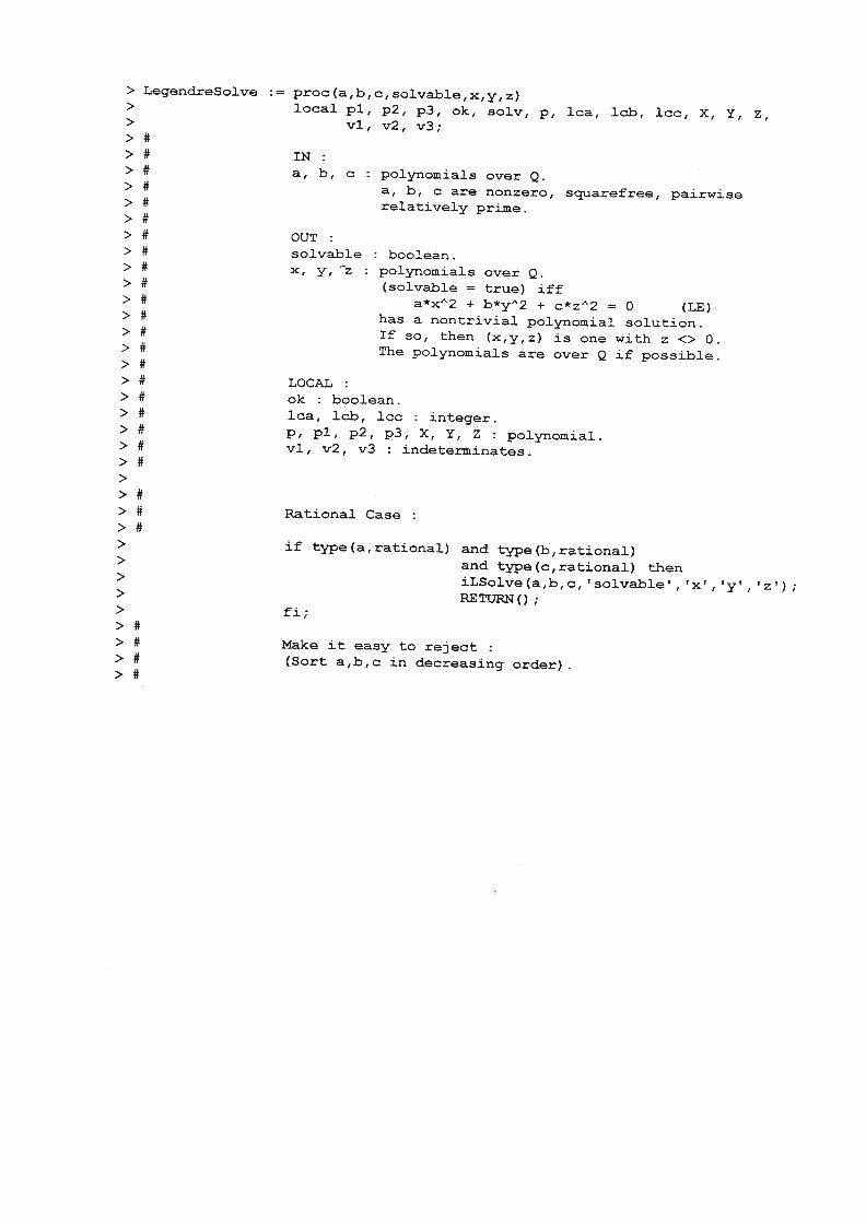
> LegendreSolve : = proc (a ,b , c, solvable, x, y, z)> local p1, p2, p3, ok, solv, p, lca, lcb, 1cc, X, Y, Z,> vi, v2, v3;>#># IN:> # a, b, c : polynomials over Q.> # a, b, c are nonzero, squarefree, pairwise> # relatively prime.>#># OUT:> # solvable : boolean.> # x, y, z : polynomials over Q.> # (solvable = true) iff> # a*x’~2 + b*yA2 + c*zA2 = 0 (LE)> # has a nontrivial polynomial solution.> # If so, then (x,y,z) is one with z <> 0.> # The polynomials are over Q if possible.>#># LOCAL:> # ok : booleari.> # ba, lob, icc : integer.> # p, p1, p2, p3, X, Y, Z : polynomial.> # vi, v2, v3 : indeterminates.>#>>#> # Rational Case>#> if type(a,rational) and type(b,rational)> and type(c,rationai) then> iLSolve(a,b,c, ‘solvable’, ‘x’, ‘y’, ‘z’)> RETtJRNO;> fi;>#> # Make it easy to reject> # (Sort a,b,c in decreasing order)>#

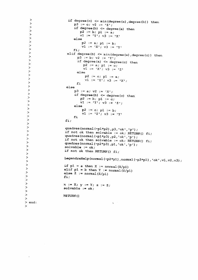
> if degree(c) <= min(degree(a),degree(b)) then

p3 := c; v2 :=> if degree(b) <= degree(a) then

p2 := b; p1 := a;vi := ‘Y’; v3 :=

> else

p2 := a; p1 := b;vi := ‘X’; v3 :=

> fi;> elif degree(b) < min(degree(a),degree(0)) then

p3 : b; v2> if degree(a) <= degree(c) then> p2 :=a;pl :=c;

vi := ‘X’; v3 :=> else> p2 :=c;pi :=a;

vi := ‘Z’; v3 := ‘X’;> fi> else> p3 := a; v2 :=

> if degree(b) <= degree(c) then> p2 :=b;pi :=c;> vi := ‘Y’; v3 :=

> else

p2 := C; p1 :=

vi := ‘Z’; v3 :=> fi> fi;>> quadres(normal(_pi*p2),p3, ‘ok’,’p’);> if not ok then solvable := ok; RETURN() fi;> quadres (normal (_pl*p3) ‘p2, ‘ok’, ‘p’);> if not ok then solvable := ok; RETTJRN() fi;> quadres (normal (_p2*p3) ,p]., ‘ok’, ‘p’);> solvable := ok;> if not ok then RETURN() fi;>> Le~endreHelp(normal(_p2*pi),flo~~l(_p3*p1) ‘ok’,vi,v2,v3);>> if p1 = a then X := normal (X/pi)> elif pi = b then Y := normal (Y/pl)> else Z := normal (Z/pi)> fi;>> x := X; y := Y; z :=

> solvable := ok;>

> RETtJRN()>> end:>

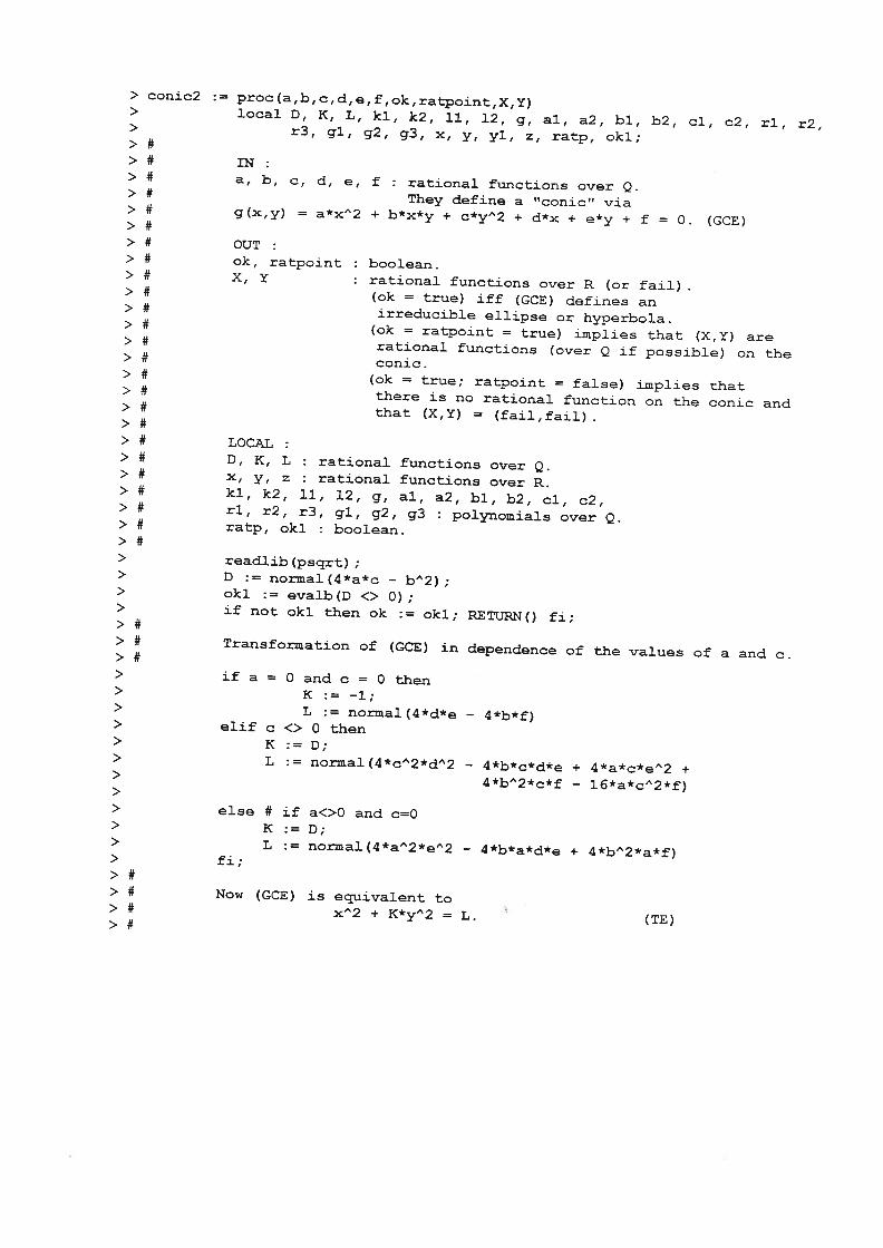
> conic2 :=

>>>>#>#>#>#>#>#>#>#>#>#>#>#>#>#>#>#>#>#>#>#>#>#>#>#>>>>>#>#>#>>>>>>>>>>>>>#>#>#>$

a, b, c, d, e,

g(x,y) = a*x”2

ok, ratpointx,Y

readlib(psqrt);D normal(4*a*c -

oki evalb(D <> 0);if not oki then ok := oki; RETURN() fi;

if a = 0 and c = 0 thenK := -1;L := normal (4*d*e - 4*b*f)

elif c <> 0 thenK := D;L := normal (4*cA2*dA2

else # if a<>0 and c=OK :=

L normal (4*aA2*eA2

Now (GCE) is equivalent toxA2 + K*yA2 = L.

OUT

proc(a,b,c,d,e,f,okratpojntXy)local D, K, L, ki, k2, 11, 12, g, ai, a2, bi, b2, ci, c2, ri, r2,

r3, gi, g2, g3, x, y, yl, z, ratp, oki;

INf : rational functions over Q.

They define a “conic” via+ b*x*y + c*yA2 + d*x + e*y + f = 0. (GCE)

boolean.rational functions over R (or fail)(Ok = true) iff (GCE) defines anirreducible ellipse or hyperbola.

(Ok = ratpoint = true) implies that (X,Y) arerational functions (over Q if possible) on theconic.

(ok = true; ratpoint = false) implies thatthere is no rational function on the conic andthat (X,Y) = (fail,fail).

LOCALD, K, L rational functions over Q.x, y, z rational functions over R.ki, k2, 11, 12, g, al, a2, bi, b2, ci, c2,ri, r2, r3, gi, g2, g3 : polynomials over Q.ratp, oki boolean.

Transformation of (CCE) in dependence of the values of a and c.

fi;

— 4*b*c*d*e + 4*a*c*eA2 +

4*bA2*c*f — i6*a*c~~2*f)

— 4*b*a*d*e + 4*bA2*a*f)

(TE)

> oki := evalb(L <> 0); # (degenerate case)> ok := oki;> if not oki then RETURN() fi;>#> # Some very special case>#> if f = 0 then ratpoint := true; X := 0; Y 0; RETURN() fi;>> ki := numer(K); k2 := denom(K);> 11 := nuxner(L); 12 := denom(L);> g := gcd(k2,12);> al normal(12*k2 / g);> bi := normal(kl*12 / g);> ci := normal(- li*k2 / g);>> oki := evalb(not( sign(lcoeff(ai)) = sign(lcoeff(bl))> and sign(lcoeff(bi)) = sign(lcoeff(ci)) ));> ok := oki;> if not oki then RETEJRN() fi;>#> # Now (TE) is equivalent to the diophantine equation> # al*x”2 + bi*yA2 + ci*zA2 = 0. (DE)>#> a2 := sqfrp(al); ri := psqrt(normal(ai/a2));> b2 := sqfrp(bl); r2 := psqrt(norxnal(bi/b2));> c2 := sqfrp(ci); r3 := psqrt(normal(cl/c2));> g := gcd(a2,gcd(b2,c2));> a2 := normal (a2/g); b2 := normal(b2/g); c2 := normal (c2/g);> gi gcd(a2,b2);> a2 := normal (a2/gi); b2 := normal(b2/gi); c2 := normal (c2*gi);> g2 gcd(a2,c2).;> a2 := normal(a2/g2); b2 := normal(b2*g2); c2 normal(c2/g2);> g3 := gcd(b2,c2);> a2 := rzormal(a2*g3); b2 := normal(b2/g3); c2 := normal (c2/g3);

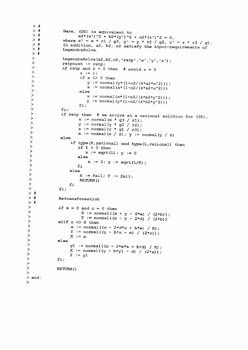
>#> # Here, (DE) is equivalent to> # a2*(xI)/~2 + b2*(y!)A2 + c2*(z’)”2 = 0,> # where x’ =x * ri / g3, yl y * r2 / g2, z’ = z * r3 / gi.> # In addition, a2, b2, c2 satisfy the input-requirements of> # Legendresolve.>#> Legendreso1ve(a2,b2,0~ ‘ratp’, ‘x’, ‘y’, ‘z’)> ratpoint := ratp;> if ratp and z = 0 then # avoid z = 0> z :=1;> ifx<>Othen> y := normal(y*(1-4-02/(4*52*XA2))).> x normal(x*(1_c2/(4*a2*xA2)))> else> x := normal(x*(1+c2/(4*b2*y~2))).> y := normal(y*(1_02/(4*b2*yA2)))> fi;> fi;> if ratp then # we arrive at a rational solution for (TE).> x normal(x * g3 / ri);> y := normal(y * g2 / r2);> z := nomal(z * gi / r3);> x := normal (x / z) ; y := normal (y / z)> else> if type(K,rational) and type(L,rational) then> ifL>Othen> x := sqrt(L); y := 0> else> x := 0; y sqrt(L/K);> fi> else> X := fail; Y := fail;

> RETtJRN()> fi> fi;>#> # Retransformation>#> ifa=Qandcothen> X := normal((x + y - 2*e) / (2*b));> Y := normal((x - y - 2*d) / (2*b))> elif o <> 0 then> x := normal((x - 2*d*c + b*e) / K);> Y := normal((y - b*x - e) / (2*c));> X:=x> else> yl := normal((x - 2*e*a + b*d) I K);> X := normal((y - b*yl - d) I (2*a));> Y:=yl> fi;>

> RETURN()>> end:>

>> conic := proc(p,var,ok,parabol,ratpointXy)> local a, b, c, d, e, f, oki, xl, yl, x, y;>#># IN:> # p : polynomial[var[1],var[2]) with coefficients from Q(t),>> # for some indeterminate t. deg(p) := 2.> # var : list of the form [van, var2j, where van, var2 are the 2> # undeterminates occuring in p.>#># OUT:> # ok, parabol, ratpoint : boolean.> # X, Y : From R(t) or “fail”.> # (ok = true) implies that g(x,y) = 0 defines an irreducible> # conic with at least two real functions on it.> # (ok = parabol = true) iff g(x,y) = 0 defines a parabola.> # (ok = ratpoint = true) implies that (X,Y) are the> # coordinates of a rational function (over Q if possible)> # on the conic.> # (Ok = true; ratpoint = false) implies that there is no> # rational function on the conic.> # g(X,Y) as function value (verification : it has to be 0).>#># LOCAL:> # a, b, c, d, e, f : rational functions over Q.> # oki : boolean.> # xl, x2 : rational functions over R or fail.> # x, y : undeterminates.>#> x := var[l]; y := var[2];> a := normal(coeff(p,xA2));> b : = normal (coeff(coeff(p,x) ,y));> c := normal(coeff(p,yA2));> d := normal(coeff(coeff(p,x),y,o));> e := normal(coeff(coeff(p,y) ,x,0));> f := normal(coeff(coeff(p,x,O) ,y, 0));

>#> # Now p = a*xF2 + b*x*y + c*zA2 ÷ d*x + e*y + f.>#> if b”2 = 4*a*c then # parabolic case> parabol := true;> Parabola(a~b,c,d,e,f,’okl~,;xlI,~yl~);> ok := okl;> if okl then> ratpoint := true;> X :=xl; Y :=yl> else> ratpoint := fail; # interpret fail as “does not matter”> X := fail; Y := fail> fi> else # ellipse/hyperbola> parabol := false;> conic2 , b, c, d, e, f, ‘okl’, ‘ratpoint’, ‘xl’ , ‘yl’)> ok :=okl;> if okl then> X :=xl; Y :=yl> else> ratpoint := fail;> X := fail; Y := fail> fi> fi;>> if oki and xl <> fail then> simplify(subs((x=xl, y=yl},p)); # test (0 as function value)> fi>> end:>

Bibliography

[BOREVICH, SHAFAREVICH 66] “Number Theory’~ by Z. I. Borevich and I. R. Sha

farevich. Academic Press, 1966.

[GEBAUER 91] “Implementation and Analysis of Parametrization

Algorithms” by Richard Gebauer (Diploma Thesis).

RISC-Linz Report Series No. 91-62, 1991.

[IRELAND, ROSEN 82] “A classical Introduction to modern Number The

ory” by K. Ireland and M. Rosen. Springer Verlag,

1982.

[KRAETZEL 81] “Zahlentheory” by E. Krätzel. VEB Dt. Verlag der

Wissenschaften, 1981.

[MORDELL 69] “Diophantine Equations” by L. J. Mordell. Aca

demic Press, 1969.

[ROSE 88] “A Course in Number Theory” by H. E. Rose. Ox

ford Science Publications, 1988.

[SCHARLAU, OPOLKA 84] “From Fermat to Minkowski” by W. Scharlau and

H. Opolka. Springer Verlag, 1984.

6L

(9661) x~dcFe o~ ‘uoT nduloD ~i~oqu1i~~ ~o J~~~~mof

JaplutM ~j pu~ ~ipuog ~j f ~q ‘~suoisua~x~ pjai~j

I~m!~dO IaAO S~An1O ~!~q~~IV ~JO~ [96 ~I~INNIM ‘V~GN~S]

(1661) I~9 - L09 d ‘9/~T uoi~nd

-moe Dr[oquI~ ~O 1~1.1r1or laPJU!JV\ ~ PU~ ~ipU~

~ f A~q ‘~~saA~rrL~ JO uOi~Zu~ur~1~d cijoquiAg~ [16 ~1~DINIM ‘v~1GN~S]