COP 4600 – Summer 2012 Introduction To Operating Systems Device Management

COP 4600: Intro To OS (Device Management) Page 1 © Dr. Mark Llewellyn

COP 4600 – Summer 2012

Introduction To Operating Systems

Device Management

Department of Electrical Engineering and Computer ScienceComputer Science DivisionUniversity of Central Florida

Instructor : Dr. Mark Llewellyn [email protected]

HEC 236, 407-823-2790http://www.cs.ucf.edu/courses/cop4600/

sum2012


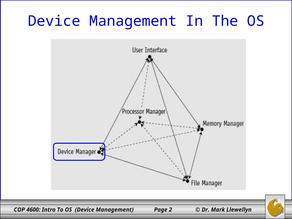
Device Management In The OS


Device Management In The OS• The Device Manager manages every peripheral device of the

system.

• Device management involves four basic functions:

1. Tracking the status of each device.

2. Using preset policies to determine which process will get a device and for how long.

3. Allocating devices to processes.

4. Deallocating devices at two levels – at the process level when an I/O command has been executed and the device is temporarily released, and at the job level when the job is finished and the device is permanently released.


Types of Devices• The system’s peripherals generally fall into one of three categories:

dedicated, shared, and virtual.• Dedicated devices are assigned to only one job at a time; they serve that

job for the entire time it is active or until it releases them. Examples are tape drives, printers, and plotters.

• Shared devices can be assigned to several different processes. For example, a disk or other direct access storage device (DASD), can be shared by several processes by interleaving their requests. The interleaving must be controlled by the Device Manager.

• Virtual devices are a combination of the first two: they’re dedicated devices that have been transformed into shared devices. For example, printers can be shared using a spooling program that reroutes print requests to a disk.


Types of Devices• The pieces of the I/O subsystem all have to work

harmoniously.

• The I/O channels play the role of dispatcher in the I/O subsystem. Their job is to keep up with the I/O requests from the CPU and pass them down the line to the appropriate control unit.

• The control unit for each device is in charge of the operations being performed on a particular I/O device.

• The I/O device itself services the request.


Types of Devices• I/O channels are programmable units placed between the CPU and the

control units. Their job is to synchronize the fast speed of the CPU with the slow speed of the I/O device, and they make it possible to overlap I/O operations with processor operations so the CPU and I/O can process concurrently.

• Channels use I/O channel programs, which can range in size from one to many instructions.

• Each channel program specifies the action to be performed by the device and controls the transmission of data between main memory and the control units.

• The channel sends one signal for each function, and the I/O control unit interprets the signal, which might say “go to the top of the page” if the device is a printer or “rewind” if the device is a tape drive.


Types of Devices• Although a control unit is sometimes part of the device, in most

systems a single control unit is attached to several similar devices, so we’ll make the distinction between the control unit and the device.

• Some systems also have a disk controller, or disk drive interface, which is a special-purpose device used to link the disk drives with the system bus.

• Disk drive interfaces control the transfer of information between the disk drives and the rest of the computer system.

• The OS normally deals only with the control and not the device.


Types of Devices• Since channels are as fast as the CPU they work with, each channel

can direct several control by interleaving commands.

• Similarly, each control unit can direct several devices.

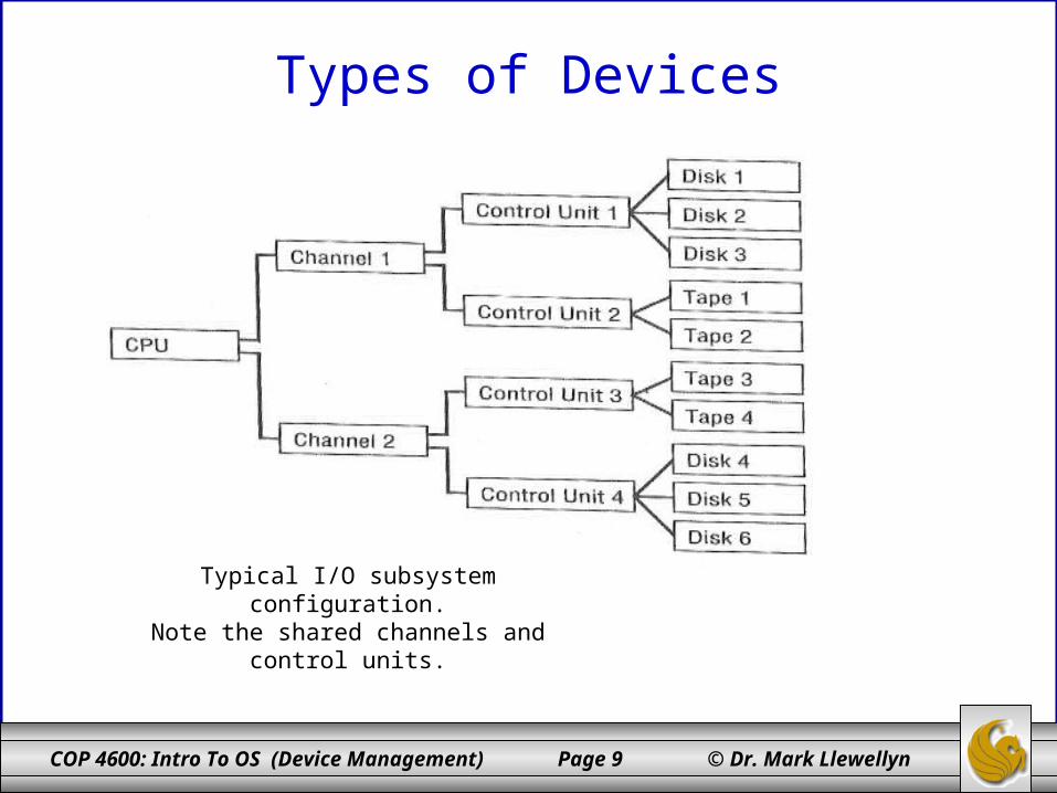
• A typical configuration might have one channel and up to eight control units, each of which communicates with up to eight I/O devices.

• Channels are often shared because they are the most expensive component in the entire I/O subsystem.

• The diagram on the next page illustrates a typical configuration. Note that the entire path be available when an I/O command is initiated.


Types of Devices

Typical I/O subsystem configuration.Note the shared channels and control units.


Types of Devices• Additional flexibility is often built into the I/O subsystem by

connecting more than one channel to a control unit, or by connecting more than one control unit to a single device.

• These multiple paths increase the reliability of the I/O subsystem by keeping communication lines open even if a component malfunctions.

• The diagram on the next page illustrates this more flexible option for the I/O subsystem configuration.


Types of Devices

Enhances I/O subsystem configuration.

Multiple paths between channels and control units as well as between control units and devices. If control unit 2 malfunctions, then tape 2 can still be accessed via control unit 3.


Storage Media Types• Storage media are divided into two groups: sequential access

storage devices (SASD) and direct access storage devices (DASD).

• SASD – This type of media stores records sequentially, one after the other. The most common form of this is magnetic tape, which originally was used for routine secondary memory, it is now used for routine archiving and storing backup data.

• DASD – This type of media can store either sequential or direct access files. Magnetic disk and optical disc drives are the most common today.


SASD – Magnetic Tape• Records on magnetic tape are stored serially, one after the other,

and each record can be of any length. The length is usually determined by the application program.

• Each record is determined by its position on the tape.

• In order to access a single record, the tape must be mounted onto a tape drive and fast-forwarded from its beginning until the desired position is located. This is a time consuming process and can take several minutes to read the entire tape, even on a fast drive.

Character representation

Parity An example of ½ inch 9 track tape – 8 tracks for character representation and 9th track used for parity bit for error checking.


SASD – Magnetic Tape• The number of character that can be recorded per inch is determined by the density of the

tape, such as 1600 or 6250 bytes per inch (bpi).

• For example, if you had records of 160 characters (bytes) each and were storing them on a tape with a density of 1600 bpi, then theoretically you could store 10 records on one linear inch of tape. Tapes typically being 2400 feet long.

• In actual practice, though, it would depend on how you store the records, individually or grouped into blocks.

• If records are stored individually, each record would be separated by a space to indicate its beginning and ending position.

• If records are stored in blocks, then the entire block is preceded by a space and followed by a space, but the individual records are stored sequentially without spaces in the block.


SASD – Magnetic TapeR

eco

rd 1

IRG

Re

cord

2

IRG

Re

cord

3

IRG

Re

cord

4

IRG

Re

cord

5

Re

cord

1

IBG

Re

cord

2

Re

cord

3

Re

cord

4

IBG

Re

cord

5

Re

cord

6

Re

cord

7

Re

cord

8

Re

cord

9

Re

cord

10

Re

cord

11

Re

cord

12

1 block of 10 records

The inter-record gap (IRG) is about ½ inch on most tapes, so using our example of 10 records/inch of tape, we’d have 9 IRGs separating 10 records and thus use a total of 5-1/2 inches of tape ( 1 inch of data needs 5-1/2 inches of tape)!

Individual records

Blocked records

The inter-block gap (IBG) is still about ½ inch on most tapes, so using our example of 10 records/inch of tape, we’d have 1 9 IBG separating 10 records and thus use a total of 1-1/2 inches of tape ( 1 inch of data needs 1-1/2 inches of tape).


SASD – Magnetic Tape• How long does it take to access a block or record on magnetic tape?• It depends on where the record is located.

Example

A 2400 foot long tape with a transport speed of 200 in/s can be read without stopping in about 2-1/2 minutes.

Thus it would take about 2-1/2 minutes to read the last record on the tape, 1-1/4 minutes on average.

Sequential access would take as long as it takes to start and stop the tape – which is about 3 ms.

• Thus, magnetic tape exhibits a high variance in access time, which makes it a poor medium for routine secondary storage, except for files with very high sequential activity, i.e., 90-100% of the records are accessed sequentially during an application.


DASD Devices• DASDs are devices that can directly read or write to a specific place

on a disk.

• Most DASDs have movable read/write heads, 1 per surface.

• Some DASDs have fixed read/write heads, 1 per track. These are very fast devices and also very expensive. They also suffer from a reduced capacity when compared to a movable head DASD (because the tracks must be positioned further apart to accommodate the width of the read/write heads). Fixed head DASDs are used when speed is of the utmost importance, such as in spacecraft monitoring and aircraft applications.

• Movable head DASDs are most common and an example is shown on the next page.


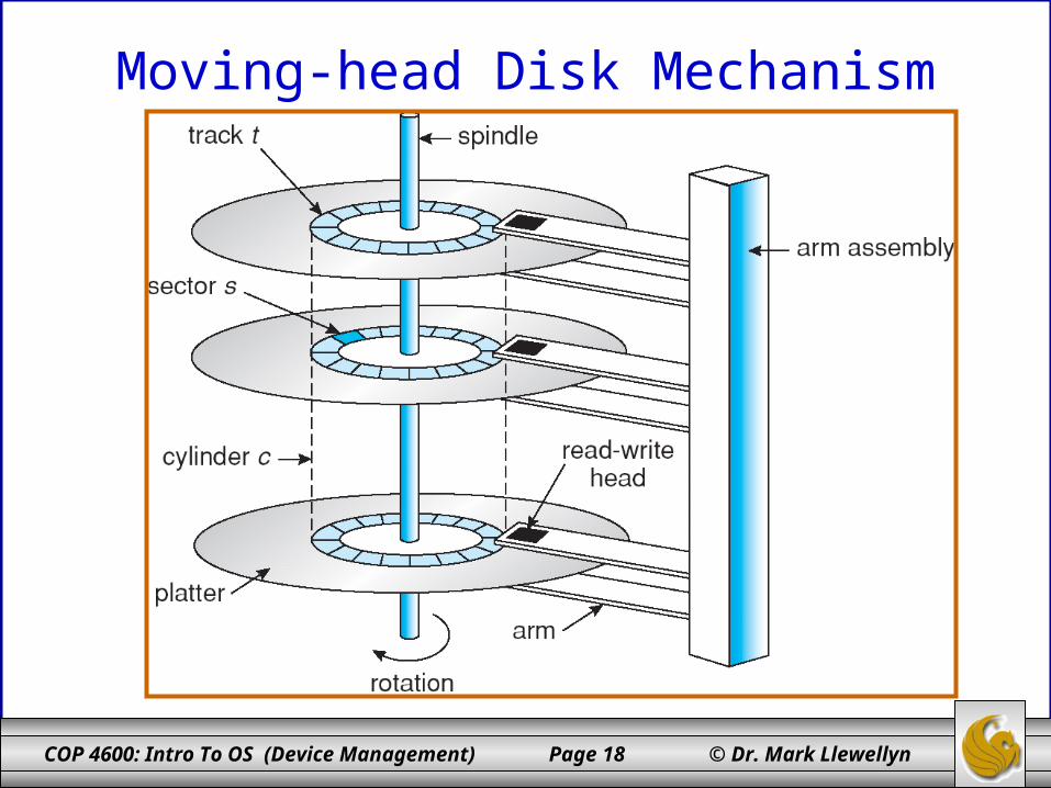
Moving-head Disk Mechanism


DASD Devices• Movable head DASDs have any where from 100 to thousands of

tracks per surface.

• Track 0 is the outmost concentric circle on each surface and the highest numbered track is in the center.

• All read/write heads are positioned over the same track simultaneously.

• It is slower to fill a disk pace surface-by-surface that it is to fill it up track-by-track.

• Filling a track on all surfaces produces a virtual cylinder of data (as shown on the previous page).

• To access any given record, the system needs three things: its cylinder number, a surface number, and a record number.


Optical Disc Storage• The advent of optical discs was made possible by developments in

laser technology.

• Laserdiscs, developed in the early 1970s, were not a big commercial success in the consumer market, although they were used for industrial training purposes.

• Audio CD, with its better sound quality, convenience, and durability, became a great success when introduced in the early 1980s.

• A fundamental difference between an optical disc and a magnetic disk is the track and sector design.

• A magnetic disk consists of concentric tracks of sectors, and it spins at a constant angular velocity (CAV). Because the sectors at the outside of the disk spin faster past the R/W head than the inner sectors, outside sectors are larger than inner sectors.


Optical Disc Storage• This format wastes space, but maximizes the speed with which

data can be retrieved.


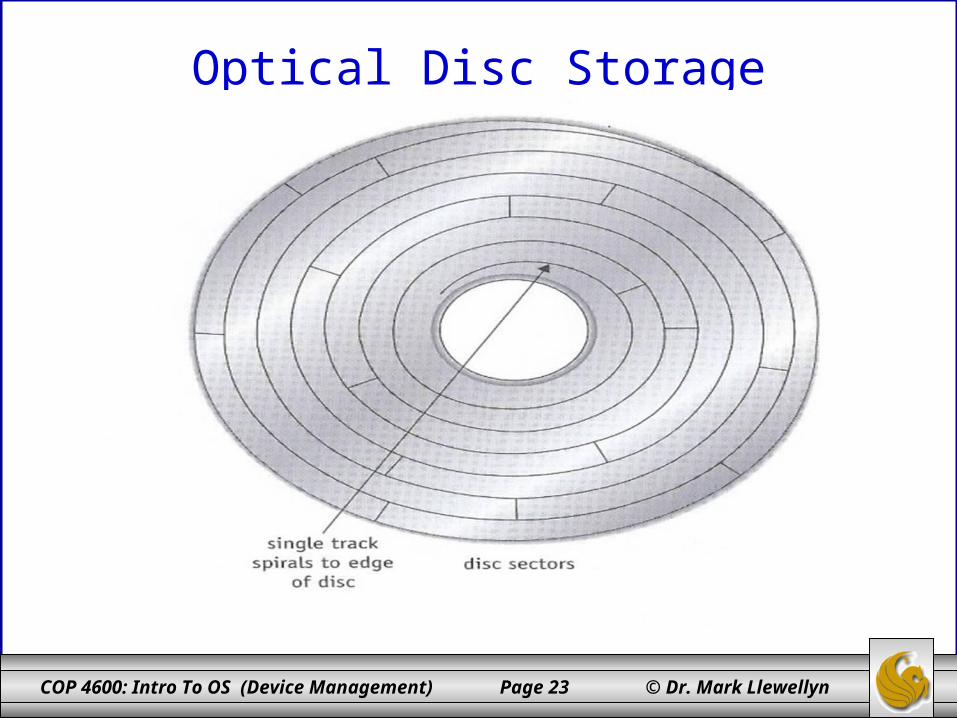
Optical Disc Storage• On the other hand, an optical disc consists of a single spiraling

track of same-sized sectors running from the center to the rim of the disc.

• This design allows many more sectors, and much more data to fit on an optical disc compared to a magnetic disk.

• If the track could be straightened on a single-sided, single layer optical disc, it would be just over 3 miles long!

• The disc drive adjusts the speed of the disc’s spin to compensate for the sector’s location on the disc. The is called constant linear velocity (CLV). Therefore, the disc spins faster to read sectors located near the center of the disc, and slower to read sectors near the outer edge. If you listen to a CD drive in action, you can hear it change speeds as it makes these adjustments.


Optical Disc Storage


Optical Disc Storage• Two of the most important measures of optical disc drive

performance are sustained data-transfer rate and average access time.

• The data transfer rate is measured in megabytes per second (MBps) and refers to the speed at which massive amounts of data can be read from the disc. This factor is crucial to applications that require sequential access, such as for audio and video playback.– For example, a CD with a fast transfer rate will drop fewer frames when

playing back a recorded video segment than will a unit with a slower transfer rate. This creates an image that is much smoother.

• The drive’s access time is more critical when retrieving data randomly. Access time is the time required to move the R/W head to a specific place on the disc. It is expressed in milliseconds.


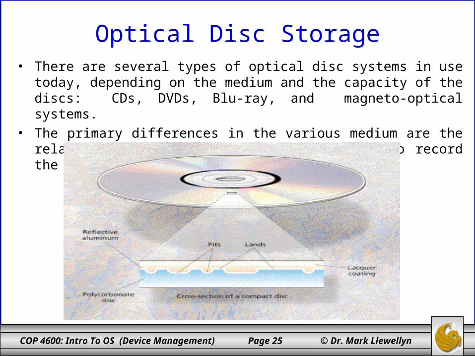
Optical Disc Storage• There are several types of optical disc systems in use today, depending on the

medium and the capacity of the discs: CDs, DVDs, Blu-ray, and magneto-optical systems.

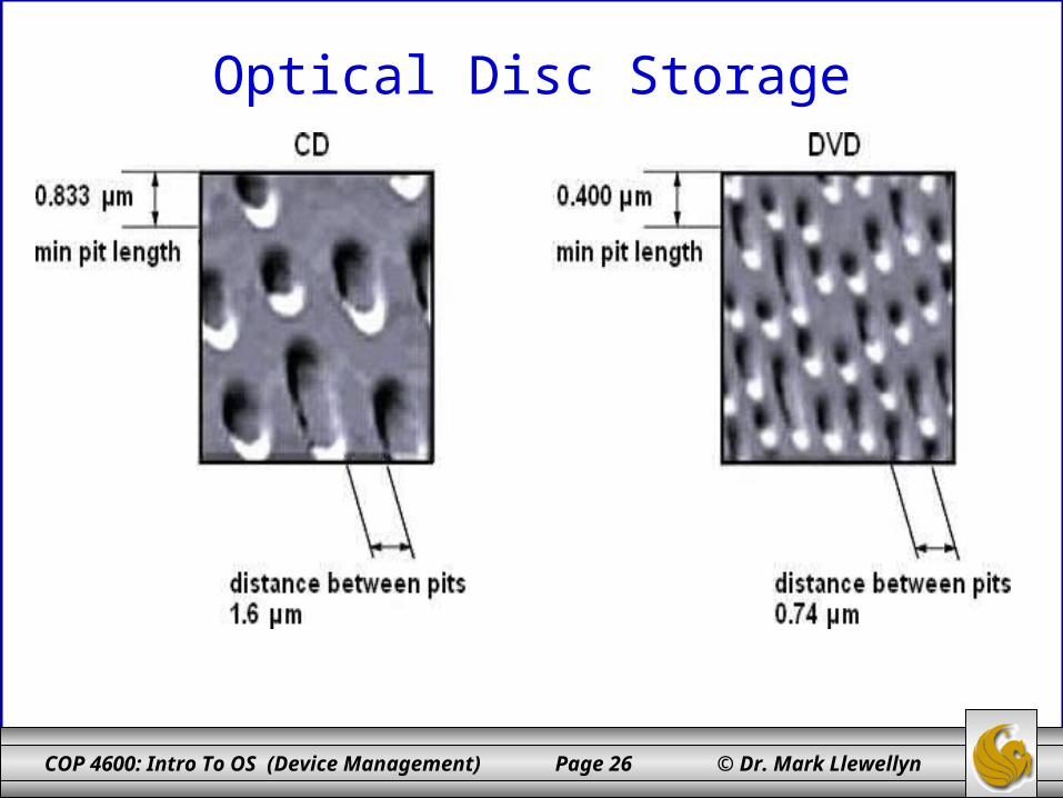
• The primary differences in the various medium are the relative sizes of the pits and lands used to record the information onto the disc.


Optical Disc Storage


DASD Access Times• Depending on whether a DASD has fixed or movable heads,

there can be as many as three factors that contribute to the time required to access a record: seek time, rotational delay, and transfer time.

• Seek time is usually the longest of the three factors. It is the time required to position the R/W head on the proper track (does not apply to fixed head DASD).

• Rotational delay is the time required to rotate the DASD until the requested record is under the R/W head.

• Transfer time is the fastest of the three, this is the time taken to actually transfer the record into main memory.


DASD Access Times• To compare the various types of DASDs on access time, let’s

assume a DASD with a time for one revolution of 16.8 ms, giving an average rotational delay of 8.4 ms.

• Seek time is normally around 50 ms for most common movable head DASDs.

• Transfer rates will vary from device to device but a typical value would be 0.00094 ms per byte. Assuming a record of 100 bytes, this would require 0.094 ms (about 0.1 ms) to transfer the record to main memory.


DASD Access Times• For fixed head DASDs:

– Access time = rotational delay + transfer time

• For movable head DASDs:

– Access time = seek time + rotational delay + transfer time

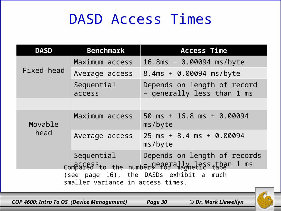
• The table on the next page illustrates the maximum access time, the average access time, and time to access sequential records for both a fixed head and a movable head DASD.


DASD Access Times

DASD Benchmark Access Time

Fixed headMaximum access 16.8ms + 0.00094 ms/byte

Average access 8.4ms + 0.00094 ms/byte

Sequential access Depends on length of record – generally less than 1 ms

Movable headMaximum access 50 ms + 16.8 ms + 0.00094 ms/byte

Average access 25 ms + 8.4 ms + 0.00094 ms/byte

Sequential access Depends on length of records – generally less than 1 ms

Compared to the numbers for magnetic tape (see page 16), the DASDs exhibit a much smaller variance in access times.


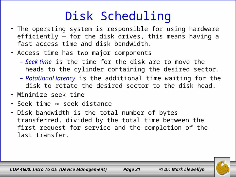
Disk Scheduling• The operating system is responsible for using hardware efficiently — for

the disk drives, this means having a fast access time and disk bandwidth.• Access time has two major components

– Seek time is the time for the disk are to move the heads to the cylinder containing the desired sector.

– Rotational latency is the additional time waiting for the disk to rotate the desired sector to the disk head.

• Minimize seek time• Seek time seek distance• Disk bandwidth is the total number of bytes transferred, divided by the

total time between the first request for service and the completion of the last transfer.


Disk Scheduling

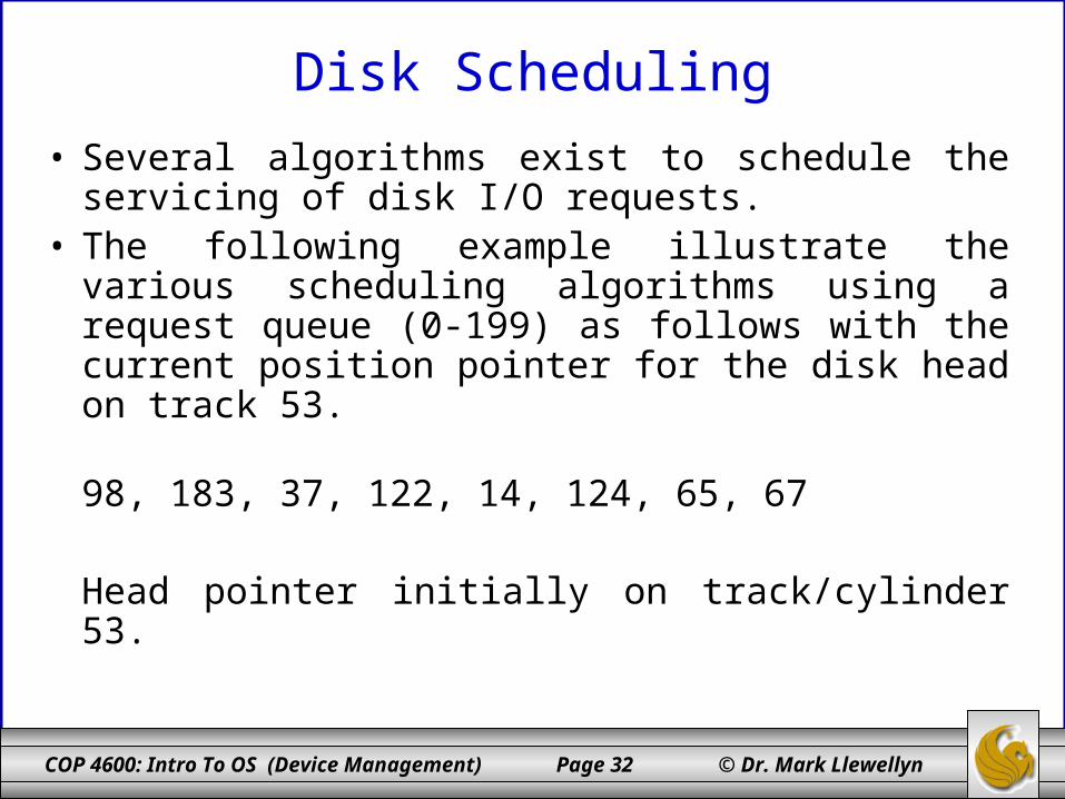
• Several algorithms exist to schedule the servicing of disk I/O requests.

• The following example illustrate the various scheduling algorithms using a request queue (0-199) as follows with the current position pointer for the disk head on track 53.

98, 183, 37, 122, 14, 124, 65, 67

Head pointer initially on track/cylinder 53.


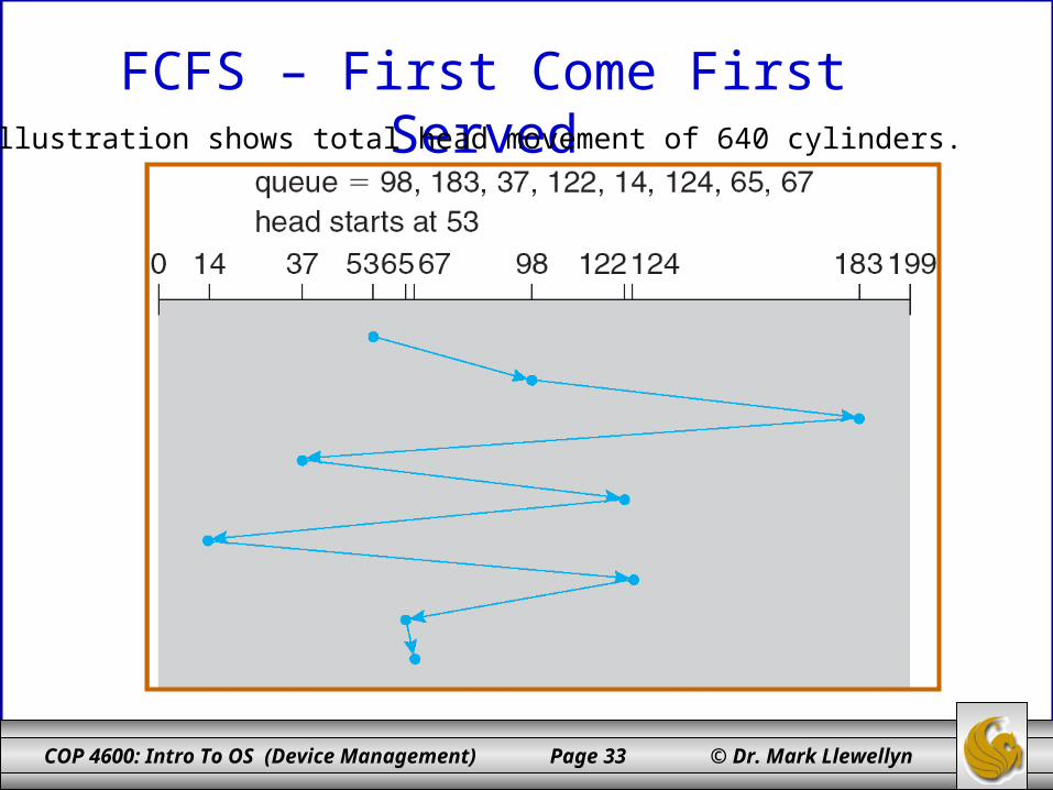
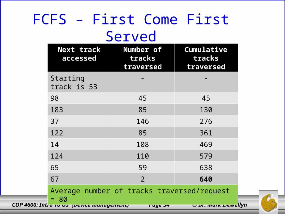
FCFS – First Come First ServedIllustration shows total head movement of 640 cylinders.


FCFS – First Come First Served

Next track accessed

Number of tracks traversed

Cumulative tracks traversed

Starting track is 53 - -

98 45 45

183 85 130

37 146 276

122 85 361

14 108 469

124 110 579

65 59 638

67 2 640

Average number of tracks traversed/request = 80


SSTF – Shortest Seek Time First

• Selects the request with the minimum seek time from the current head position.

• SSTF scheduling is a form of SJF scheduling; may cause starvation of some requests.

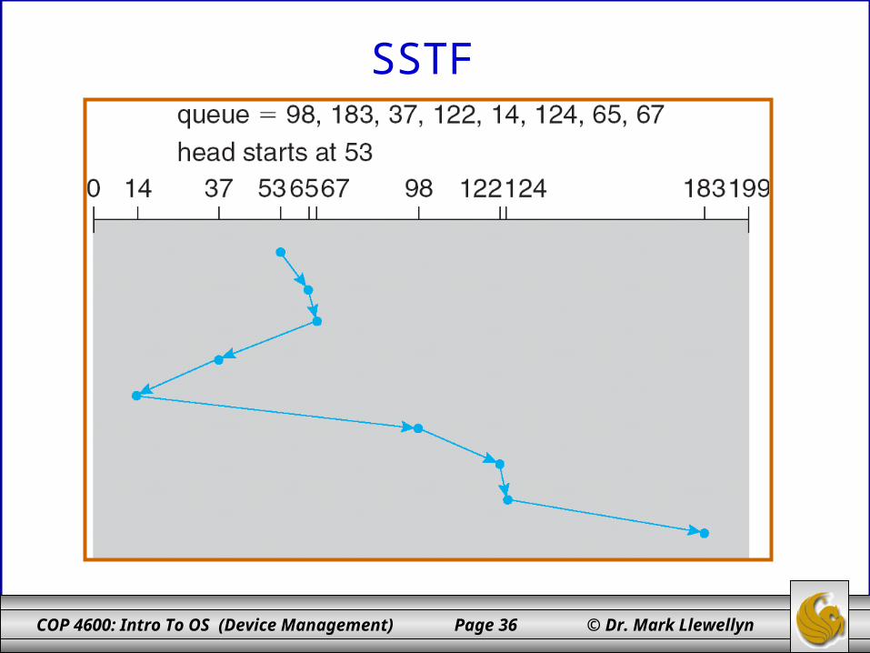
• Again if we assume that the read/write head is initially position over track/cylinder 53, then the illustration on the next page shows a total head movement of 236 cylinders.


SSTF


SSTF – Shortest Seek Time First

Next track accessed

Number of tracks traversed

Cumulative tracks traversed

Starting track is 53 - -

65 12 12

67 2 14

37 30 44

14 23 67

98 84 151

122 24 175

124 2 177

183 59 236

Average number of tracks traversed = 29.5


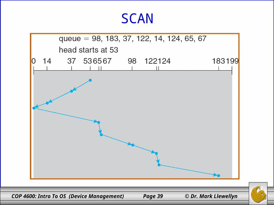
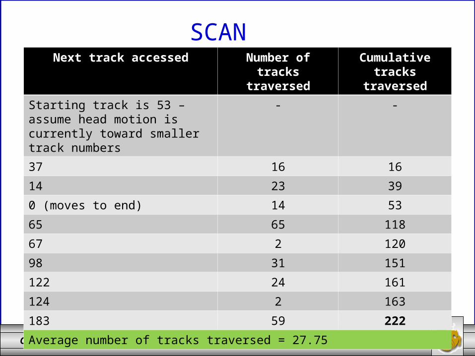
SCAN – Elevator Algorithm• The disk arm starts at one end of the disk, and moves

toward the other end, servicing requests until it gets to the other end of the disk, where the head movement is reversed and servicing continues.

• Sometimes called the elevator algorithm.

• Again, assuming the read/write head is currently positioned on track 53 and the head is moving toward smaller track numbers, the illustration on the next page shows a total head movement of 222 cylinders.


SCAN


SCANNext track accessed Number of tracks

traversedCumulative tracks

traversed

Starting track is 53 – assume head motion is currently toward smaller track numbers

- -

37 16 16

14 23 39

0 (moves to end) 14 53

65 65 118

67 2 120

98 31 151

122 24 161

124 2 163

183 59 222



SCANNext track accessed Number of tracks


traversed

Starting track is 53 – assume head motion is currently toward larger track numbers

- -

65 12 12

67 2 14

98 31 45

122 24 69

124 2 71

183 59 130

199 (moves to the end) 16 146

37 162 308

14 23 331



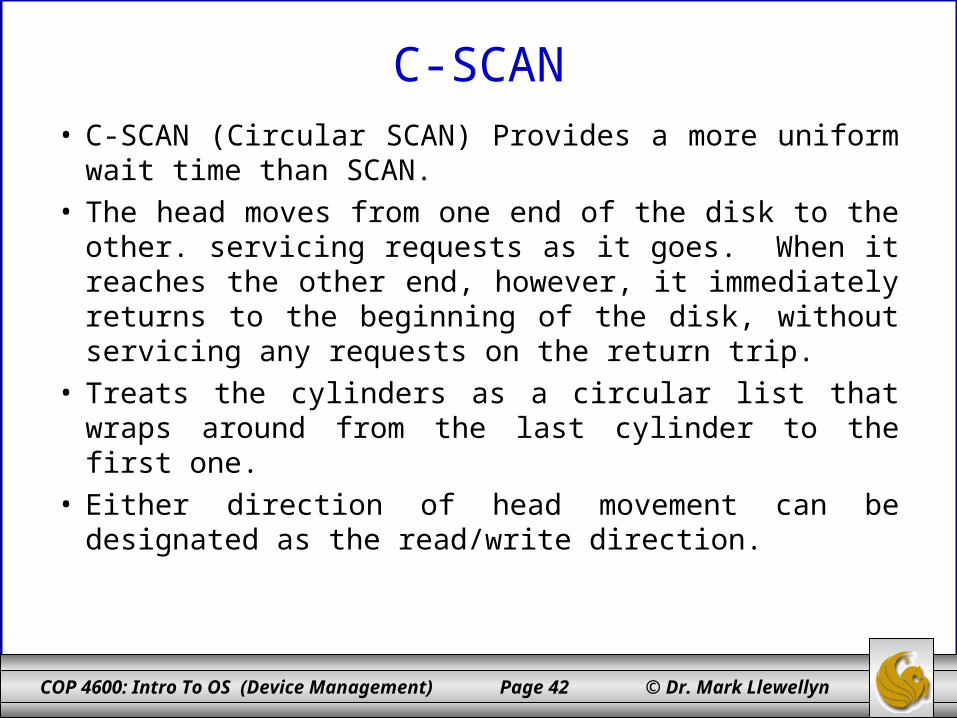
C-SCAN

• C-SCAN (Circular SCAN) Provides a more uniform wait time than SCAN.

• The head moves from one end of the disk to the other. servicing requests as it goes. When it reaches the other end, however, it immediately returns to the beginning of the disk, without servicing any requests on the return trip.

• Treats the cylinders as a circular list that wraps around from the last cylinder to the first one.

• Either direction of head movement can be designated as the read/write direction.


C-SCAN

R/W direction is toward larger track numbers


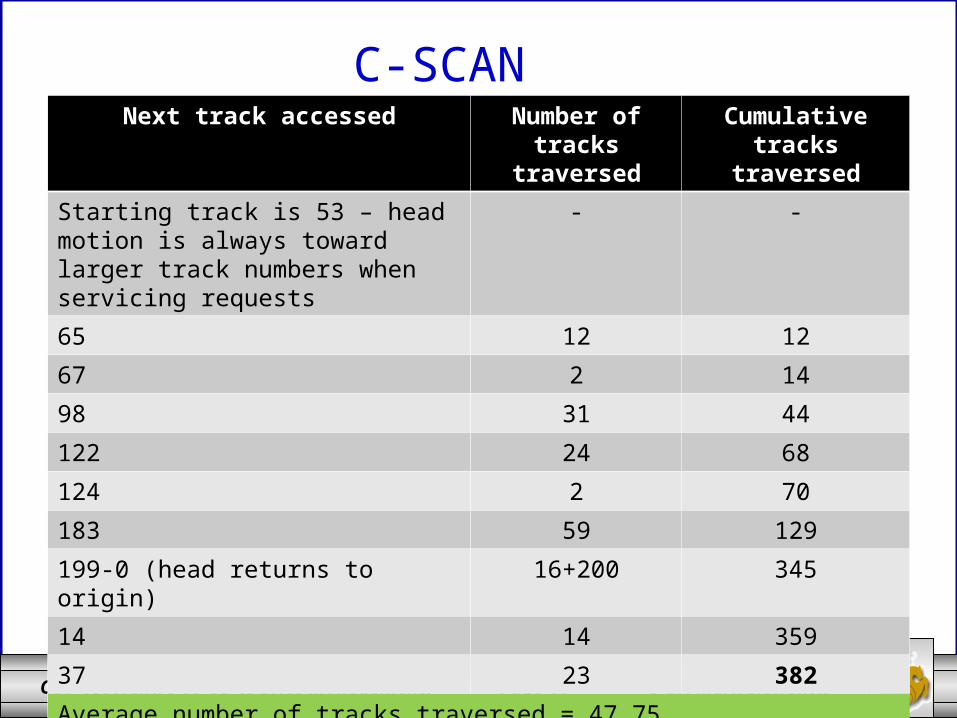
C-SCANNext track accessed Number of tracks


traversed

Starting track is 53 – head motion is always toward larger track numbers when servicing requests

- -

65 12 12

67 2 14

98 31 44

122 24 68

124 2 70

183 59 129

199-0 (head returns to origin) 16+200 345

14 14 359

37 23 382



C-SCANNext track accessed Number of tracks


traversed

Starting track is 53 – head motion is always toward smaller track numbers when servicing requests

- -

37 16 16

14 23 39

0-199 (moves to end) 14+200 253

183 16 269

124 59 328

122 2 330

98 24 354

67 31 385

65 2 387



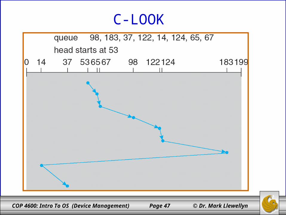
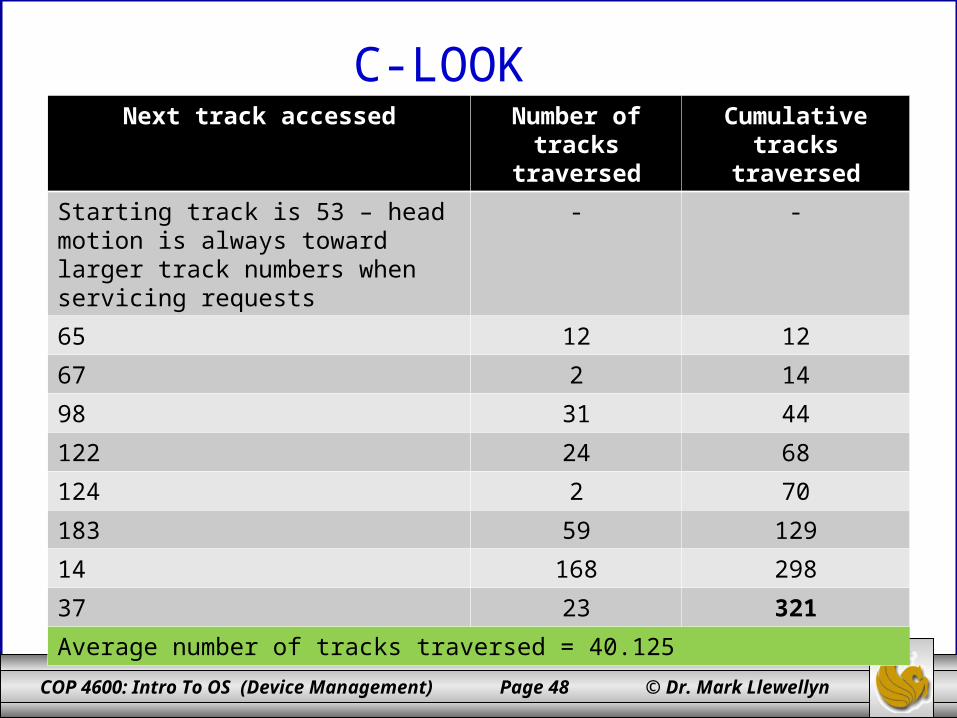
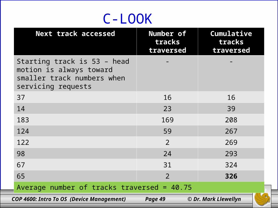
C-LOOK

• Version of C-SCAN

• Arm only goes as far as the last request in each direction, then reverses direction immediately, without first going all the way to the end of the disk.


C-LOOK


C-LOOKNext track accessed Number of tracks


traversed

Starting track is 53 – head motion is always toward larger track numbers when servicing requests

- -

65 12 12

67 2 14

98 31 44

122 24 68

124 2 70

183 59 129

14 168 298

37 23 321



C-LOOKNext track accessed Number of tracks


traversed

Starting track is 53 – head motion is always toward smaller track numbers when servicing requests

- -

37 16 16

14 23 39

183 169 208

124 59 267

122 2 269

98 24 293

67 31 324

65 2 326



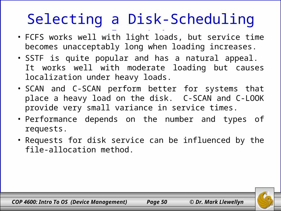
Selecting a Disk-Scheduling Algorithm• FCFS works well with light loads, but service time becomes

unacceptably long when loading increases.

• SSTF is quite popular and has a natural appeal. It works well with moderate loading but causes localization under heavy loads.

• SCAN and C-SCAN perform better for systems that place a heavy load on the disk. C-SCAN and C-LOOK provide very small variance in service times.

• Performance depends on the number and types of requests.

• Requests for disk service can be influenced by the file-allocation method.


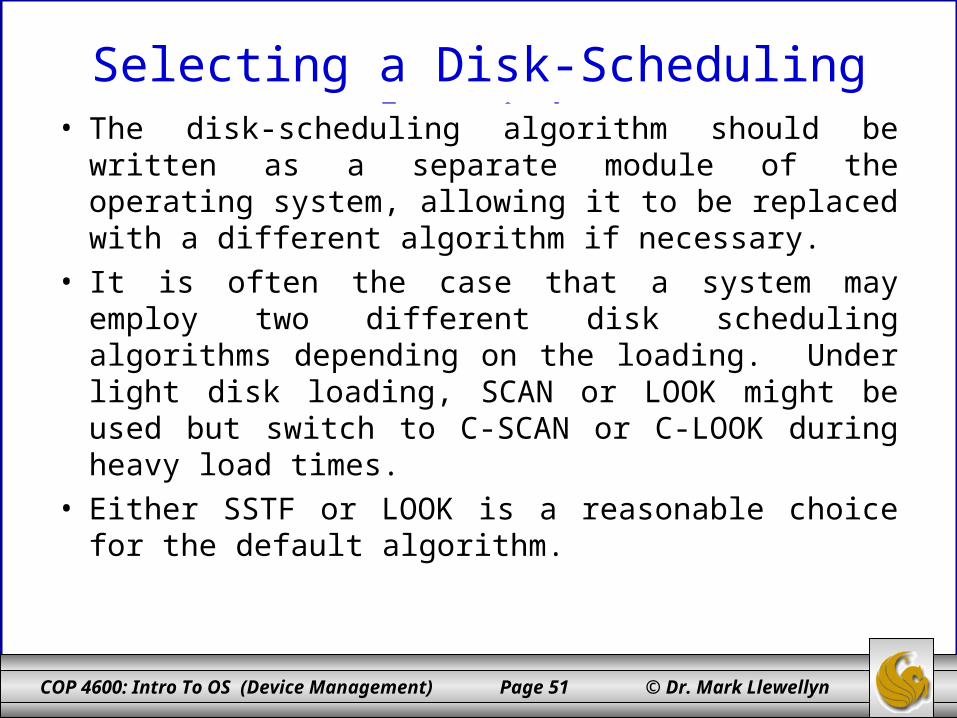
Selecting a Disk-Scheduling Algorithm• The disk-scheduling algorithm should be written as a

separate module of the operating system, allowing it to be replaced with a different algorithm if necessary.

• It is often the case that a system may employ two different disk scheduling algorithms depending on the loading. Under light disk loading, SCAN or LOOK might be used but switch to C-SCAN or C-LOOK during heavy load times.

• Either SSTF or LOOK is a reasonable choice for the default algorithm.


RAID• RAID is a set of physical disk drives that is viewed as a single

logical unit by the OS.

• RAID was introduced to close the widening gap between increasingly fast processors and slower disk drives.

• RAID assumes that several smaller capacity disk drives are preferable to a few large-capacity drives because, by distributing the data among several smaller disks, the system can simultaneously access the requested data from the multiple drives, resulting in improved I/O performance and improved data recovery in the event of disk failure.

• A typical disk array configuration is shown on the next page .


RAID Levels (cont.)

Raid 0


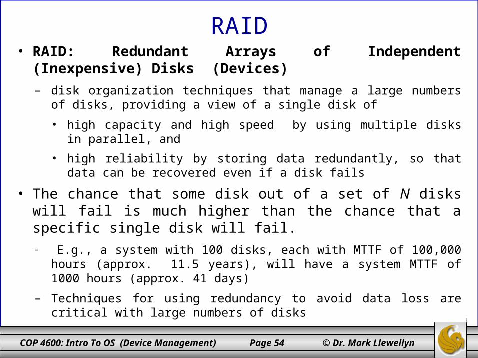
RAID• RAID: Redundant Arrays of Independent (Inexpensive) Disks

(Devices)

– disk organization techniques that manage a large numbers of disks, providing a view of a single disk of

• high capacity and high speed by using multiple disks in parallel, and

• high reliability by storing data redundantly, so that data can be recovered even if a disk fails

• The chance that some disk out of a set of N disks will fail is much higher than the chance that a specific single disk will fail.

– E.g., a system with 100 disks, each with MTTF of 100,000 hours (approx. 11.5 years), will have a system MTTF of 1000 hours (approx. 41 days)

– Techniques for using redundancy to avoid data loss are critical with large numbers of disks


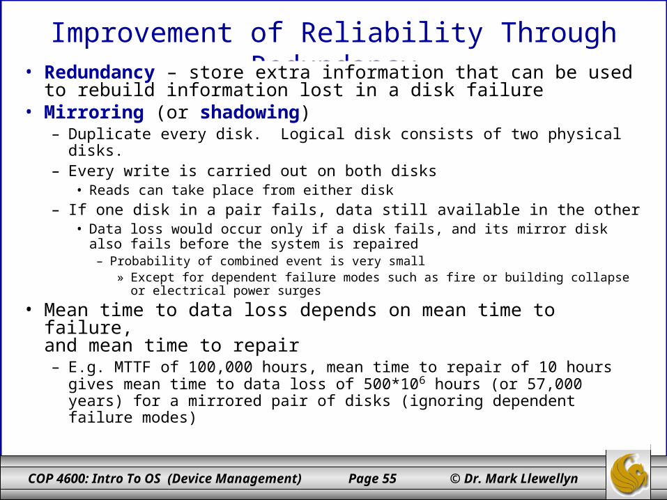
Improvement of Reliability Through Redundancy• Redundancy – store extra information that can be used to rebuild

information lost in a disk failure• Mirroring (or shadowing)

– Duplicate every disk. Logical disk consists of two physical disks.– Every write is carried out on both disks

• Reads can take place from either disk

– If one disk in a pair fails, data still available in the other• Data loss would occur only if a disk fails, and its mirror disk also fails before the

system is repaired– Probability of combined event is very small

» Except for dependent failure modes such as fire or building collapse or electrical power surges

• Mean time to data loss depends on mean time to failure, and mean time to repair– E.g. MTTF of 100,000 hours, mean time to repair of 10 hours gives mean

time to data loss of 500*106 hours (or 57,000 years) for a mirrored pair of disks (ignoring dependent failure modes)


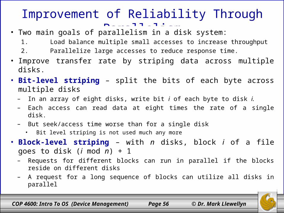
Improvement of Reliability Through Parallelism

• Two main goals of parallelism in a disk system: 1. Load balance multiple small accesses to increase throughput

2. Parallelize large accesses to reduce response time.

• Improve transfer rate by striping data across multiple disks.

• Bit-level striping – split the bits of each byte across multiple disks– In an array of eight disks, write bit i of each byte to disk i.

– Each access can read data at eight times the rate of a single disk.

– But seek/access time worse than for a single disk• Bit level striping is not used much any more

• Block-level striping – with n disks, block i of a file goes to disk (i mod n) + 1– Requests for different blocks can run in parallel if the blocks reside on

different disks

– A request for a long sequence of blocks can utilize all disks in parallel


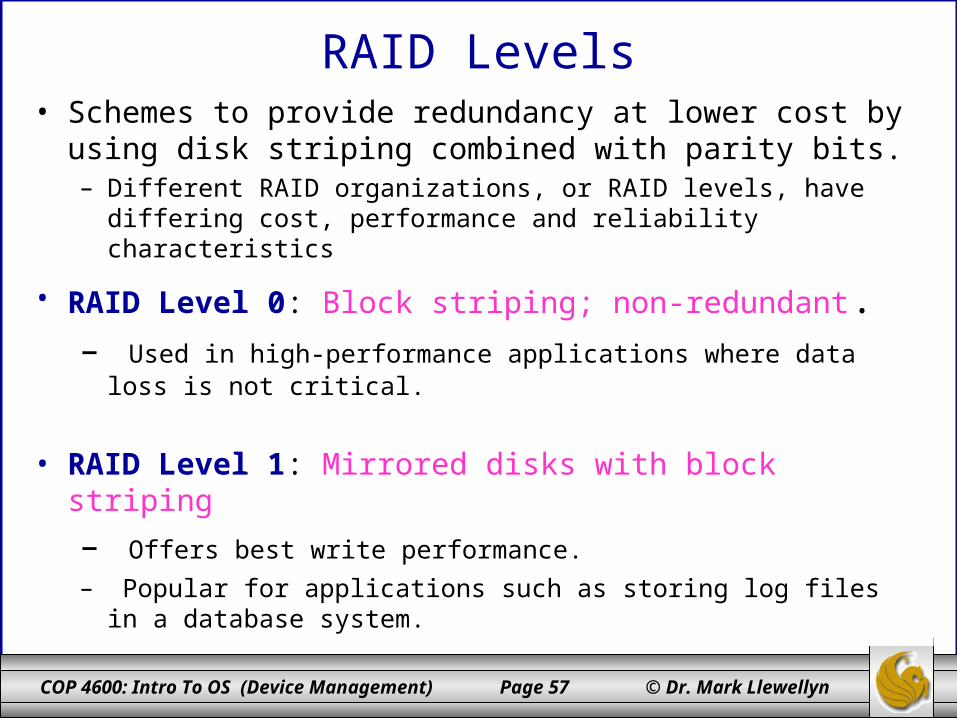
RAID Levels• Schemes to provide redundancy at lower cost by using disk

striping combined with parity bits.– Different RAID organizations, or RAID levels, have differing cost,

performance and reliability characteristics

• RAID Level 0: Block striping; non-redundant. – Used in high-performance applications where data loss is not critical.

• RAID Level 1: Mirrored disks with block striping

– Offers best write performance.

– Popular for applications such as storing log files in a database system.


RAID Levels (cont.)

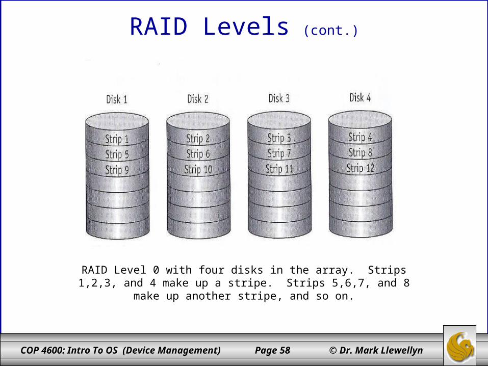
RAID Level 0 with four disks in the array. Strips 1,2,3, and 4 make up a stripe. Strips 5,6,7, and 8 make up another stripe, and so on.


RAID Levels (cont.)

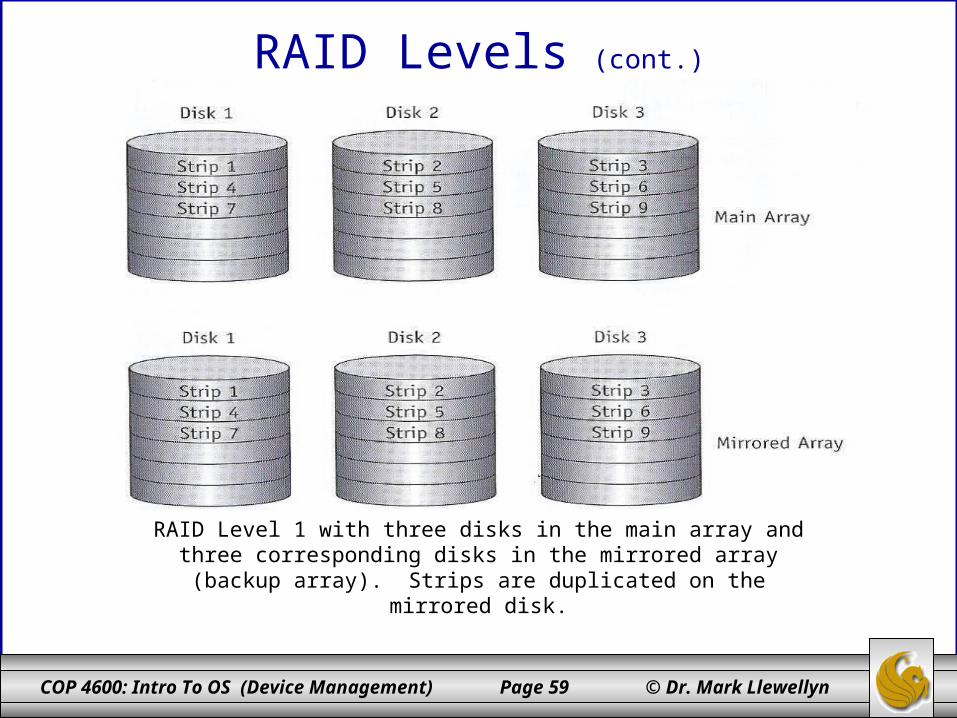
RAID Level 1 with three disks in the main array and three corresponding disks in the mirrored array (backup array). Strips are

duplicated on the mirrored disk.


RAID Levels (cont.)

• RAID Level 2: Memory-Style Error-Correcting-Codes (ECC) with bit striping.

• RAID Level 3: Bit-Interleaved Parity

– A single parity bit is enough for error correction, not just detection, since we know which disk has failed

• When writing data, corresponding parity bits must also be computed and written to a parity bit disk

• To recover data in a damaged disk, compute XOR of bits from other disks (including parity bit disk)

– Faster data transfer than with a single disk, but fewer I/Os per second since every disk has to participate in every I/O.

– Subsumes Level 2 (provides all its benefits, at lower cost).


RAID Levels (cont.)

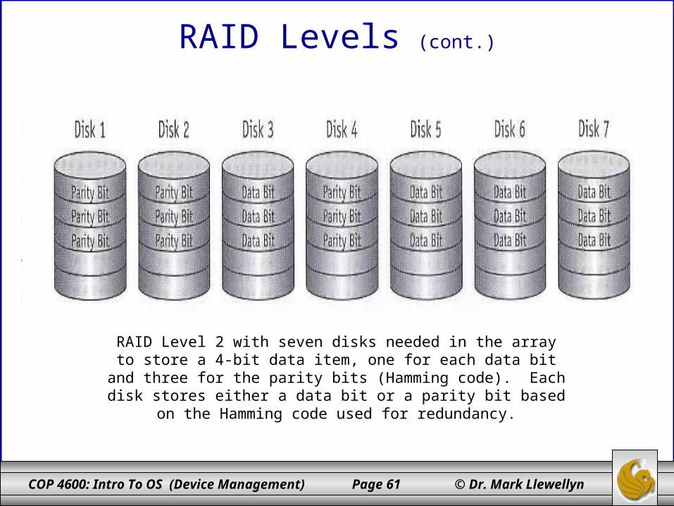
RAID Level 2 with seven disks needed in the array to store a 4-bit data item, one for each data bit and three for the parity bits

(Hamming code). Each disk stores either a data bit or a parity bit based on the Hamming code used for redundancy.


RAID Levels (cont.)

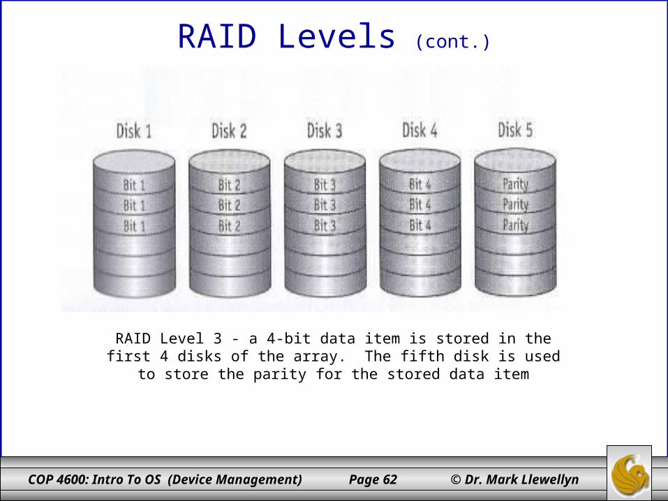
RAID Level 3 - a 4-bit data item is stored in the first 4 disks of the array. The fifth disk is used to store the parity for the stored data

item


RAID Levels (cont.)

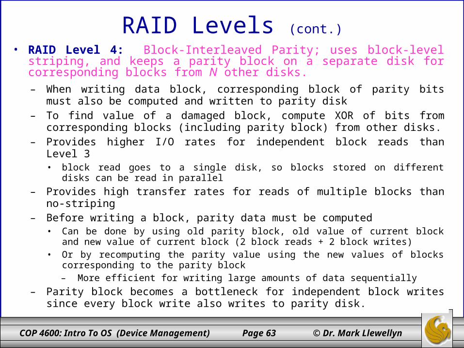
• RAID Level 4: Block-Interleaved Parity; uses block-level striping, and keeps a parity block on a separate disk for corresponding blocks from N other disks.

– When writing data block, corresponding block of parity bits must also be computed and written to parity disk

– To find value of a damaged block, compute XOR of bits from corresponding blocks (including parity block) from other disks.

– Provides higher I/O rates for independent block reads than Level 3 • block read goes to a single disk, so blocks stored on different disks can be read in parallel

– Provides high transfer rates for reads of multiple blocks than no-striping– Before writing a block, parity data must be computed

• Can be done by using old parity block, old value of current block and new value of current block (2 block reads + 2 block writes)

• Or by recomputing the parity value using the new values of blocks corresponding to the parity block

– More efficient for writing large amounts of data sequentially

– Parity block becomes a bottleneck for independent block writes since every block write also writes to parity disk.


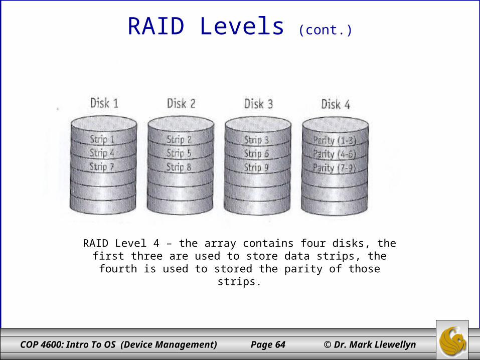
RAID Levels (cont.)

RAID Level 4 – the array contains four disks, the first three are used to store data strips, the fourth is used to stored the parity of those

strips.


RAID Levels (cont.)

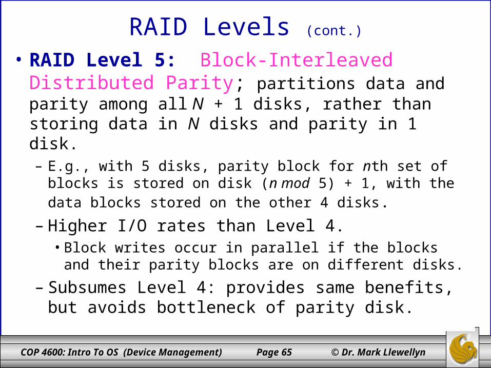
• RAID Level 5: Block-Interleaved Distributed Parity; partitions data and parity among all N + 1 disks, rather than storing data in N disks and parity in 1 disk.– E.g., with 5 disks, parity block for nth set of blocks is stored on

disk (n mod 5) + 1, with the data blocks stored on the other 4 disks.

– Higher I/O rates than Level 4. • Block writes occur in parallel if the blocks and their parity

blocks are on different disks.

– Subsumes Level 4: provides same benefits, but avoids bottleneck of parity disk.


RAID Levels (cont.)

RAID Level 5 – showing four disks. Notice how the parity strips are distributed among the disks.


Disk 1 Disk 2 Disk 3 Disk 4 Disk 5

P2 P3 P4P0 P1

Block 0 Block 1 Block 2 Block 3

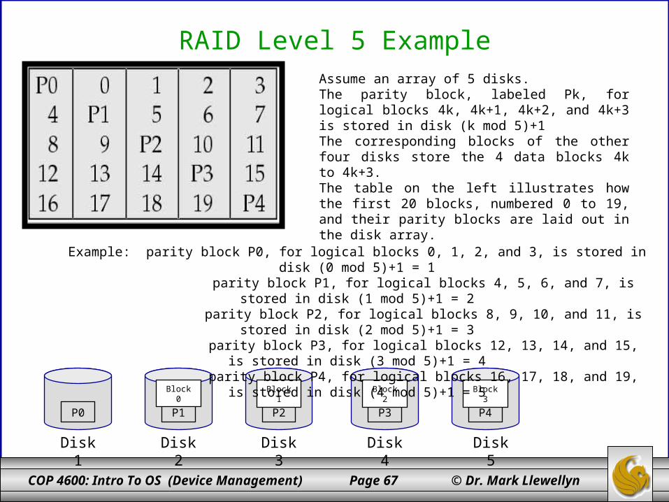
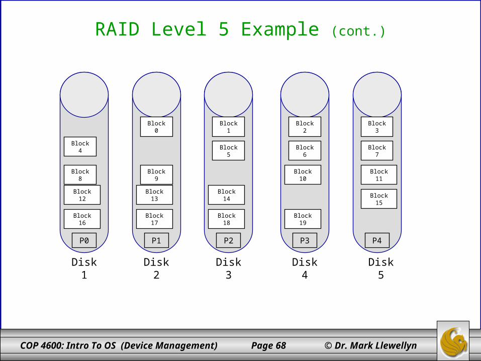
RAID Level 5 ExampleAssume an array of 5 disks.The parity block, labeled Pk, for logical blocks 4k, 4k+1, 4k+2, and 4k+3 is stored in disk (k mod 5)+1The corresponding blocks of the other four disks store the 4 data blocks 4k to 4k+3.The table on the left illustrates how the first 20 blocks, numbered 0 to 19, and their parity blocks are laid out in the disk array.

Example: parity block P0, for logical blocks 0, 1, 2, and 3, is stored in disk (0 mod 5)+1 = 1 parity block P1, for logical blocks 4, 5, 6, and 7, is stored in disk (1 mod 5)+1 = 2

parity block P2, for logical blocks 8, 9, 10, and 11, is stored in disk (2 mod 5)+1 = 3 parity block P3, for logical blocks 12, 13, 14, and 15, is stored in disk (3 mod 5)+1 = 4 parity block P4, for logical blocks 16, 17, 18, and 19, is stored in disk (4 mod 5)+1 = 5


RAID Level 5 Example (cont.)

Disk 1 Disk 2 Disk 3 Disk 4 Disk 5

P2 P3 P4P0 P1


Block 4Block 5 Block 6 Block 7


Block 12 Block 13 Block 14Block 15



RAID Levels (cont.)

• RAID Level 6: P+Q Redundancy scheme; – Similar to Level 5, but stores extra redundant information to

guard against multiple disk failures.

– Better reliability than Level 5 at a higher cost; not used as widely.


RAID Levels (cont.)

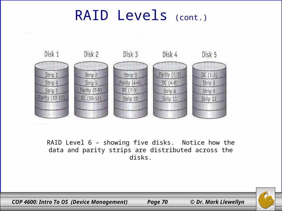
RAID Level 6 – showing five disks. Notice how the data and parity strips are distributed across the disks.


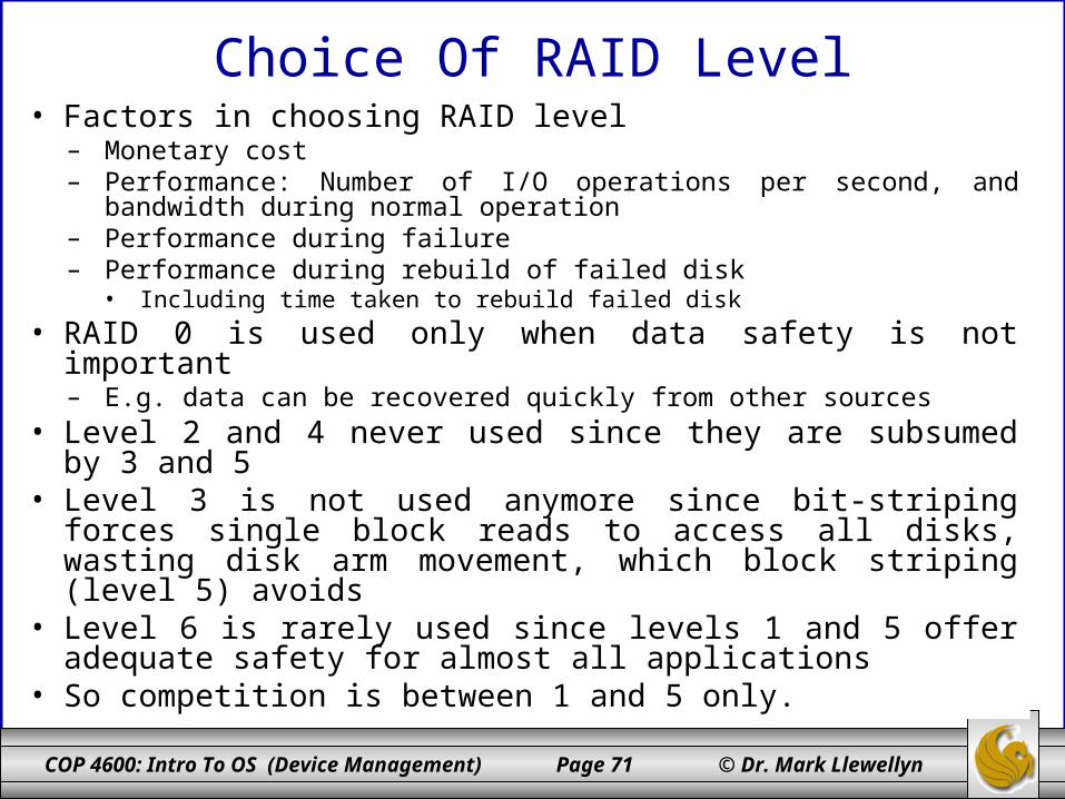
Choice Of RAID Level• Factors in choosing RAID level

– Monetary cost– Performance: Number of I/O operations per second, and bandwidth during

normal operation– Performance during failure– Performance during rebuild of failed disk

• Including time taken to rebuild failed disk

• RAID 0 is used only when data safety is not important – E.g. data can be recovered quickly from other sources

• Level 2 and 4 never used since they are subsumed by 3 and 5• Level 3 is not used anymore since bit-striping forces single block

reads to access all disks, wasting disk arm movement, which block striping (level 5) avoids

• Level 6 is rarely used since levels 1 and 5 offer adequate safety for almost all applications

• So competition is between 1 and 5 only.


Choice Of RAID Level (cont.)

• Level 1 provides much better write performance than level 5– Level 5 requires at least 2 block reads and 2 block writes to write a single

block, whereas Level 1 only requires 2 block writes

– Level 1 preferred for high update environments such as log disks

• Level 1 had higher storage cost than level 5– disk drive capacities increasing rapidly (50%/year) whereas disk access

times have decreased much less (x 3 in 10 years)

– I/O requirements have increased greatly, e.g. for Web servers

– When enough disks have been bought to satisfy required rate of I/O, they often have spare storage capacity• so there is often no extra monetary cost for Level 1!

• Level 5 is preferred for applications with low update rate,and large amounts of data

• Level 1 is preferred for all other applications


Additional RAID Levels • The single RAID levels have distinct advantages and disadvantages, which is why most

of them are used in various parts of the market to address different application requirements.

• It wasn't long after RAID began to be implemented that engineers looked at these RAID levels and began to wonder if it might be possible to get some of the advantages of more than one RAID level by designing arrays that use a combination of techniques.

• These RAID levels are called variously multiple, nested, or multi-RAID levels. They are also sometimes called two-dimensional, in reference to the two-dimensional schematics that are used to represent the application of two RAID levels to a set of disks.

• Multiple RAID levels are most commonly used to improve performance, and they do this well. Nested RAID levels typically provide better performance characteristics than either of the single RAID levels that comprise them. The most commonly combined level is RAID 0, which is often mixed with redundant RAID levels such as 1, 3 or 5 to provide fault tolerance while exploiting the performance advantages of RAID 0. There is never a "free lunch", and so with multiple RAID levels what you pay is a cost in complexity: many drives are required, management and maintenance are more involved, and for some implementations a high-end RAID controller is required.

• Not all combinations of RAID levels exist. Typically, the most popular multiple RAID levels are those that combine single RAID levels that complement each other with different strengths and weaknesses. Making a multiple RAID array marrying RAID 4 to RAID 5 wouldn't be the best idea, since they are so similar to begin with.

Documents

COP 4600 – Summer 2012 Introduction To Operating Systems Device Management