Embed Size (px)
Citation preview

8 September, 2015 Coordinated Multiantenna Interference Management in 5G Networks 1
Coordinated Multiantenna Interference Managementin 5G Networks
Antti [email protected]
Department of Communications Engineering (DCE)University of Oulu, Finland
8 September, 2015
c©Antti Tolli, Department of Comm. Engineering

8 September, 2015 Coordinated Multiantenna Interference Management in 5G Networks 2
OutlineEvolution of multiantenna systemsMIMO with large antenna arraysLinear transceiver design and resource allocation
I Introduction to convex optimisationI Resource allocation and linear transceiver designI Coordinated transceiver optimisationI Coherent vs. coordinated beamforming
Minimum power multicell beamforming with QoS constraintsI Centralised solutionI Decentralised solution via optimisation decompositionI Large system approximation
Throughput optimal linear TX-RX designI Weighted sum rate maximisation (WSRM) via MSE minimisationI WSRM with rate constraintsI Decentralised solution via precoded UL pilotI Bidirectional signalling strategies for dynamic TDDI Mode selection and transceiver design in underlay D2D MIMO
systemsc©Antti Tolli, Department of Comm. Engineering

8 September, 2015 Coordinated Multiantenna Interference Management in 5G Networks 3
Motivation
Conventional cellular systems are interference limitedI In-cell users are processed independently by each base station (BS)
I Other users are treated as inter-cell interference
I Interference mitigated by sharing and reusing available resources
Coordinated multi-node transmission with multi-user precodingI Increased spatial degrees of freedom in a multi-user MIMO channel
I A system with N distributed antennas can ideally accommodate upto N streams
I Inter-stream interference can be controlled or eliminated by a properbeamformer design.
I Coherent multi-cell MIMO: user data transmitted over a large virtualMIMO channel
c©Antti Tolli, Department of Comm. Engineering

8 September, 2015 Coordinated Multiantenna Interference Management in 5G Networks 4
General ObjectiveGoal: Design dynamic multi-dimensional radio resource managementacross time, frequency, and space (location)Assumption: Heterogeneous network composed of
I Large macro cells with massive MIMO antenna arrays,I Small cells and relays with small or distributed MIMO arrays, andI D2D communication with macro cell coordination
Backhaul / controlData
c©Antti Tolli, Department of Comm. Engineering

8 September, 2015 Coordinated Multiantenna Interference Management in 5G Networks 5
Evolution of Multiantenna Systems
!"#$%&$%$"'$(
)!)*( +!)*,)!+*( +!+*(
+-.+!+*( +-.+!+*(/(0"#$%.(
'$11(0"#$%&$%$"'$(
233%40"5#$4(6718'$11(
+-.+!+*(
c©Antti Tolli, Department of Comm. Engineering

8 September, 2015 Coordinated Multiantenna Interference Management in 5G Networks 6
Coordinated Multi-cell Transmission/Reception
Coherent (joint) multi-cell transmissionI Each data stream may be transmitted from multiple nodesI Tight synchronisation across the transmitting nodes (common carrier
phase reference)I A high-speed backbone network, e.g. Radio over Fibre
Controller
c©Antti Tolli, Department of Comm. Engineering

8 September, 2015 Coordinated Multiantenna Interference Management in 5G Networks 7
Coordinated Multi-cell Transmission/ReceptionCoordinated beamforming
I Dynamic multi-cell scheduling and inter-cell interference avoidanceI Coordinated precoder design and beam allocationI Each data stream is transmitted from a single BS nodeI No carrier phase coherence requirementI Looser requirement on the coordination and the backhaul →
Decentralized processing
Controller
c©Antti Tolli, Department of Comm. Engineering

8 September, 2015 Coordinated Multiantenna Interference Management in 5G Networks 8
Interference AlignmentConsider a symmetric constant MIMO interference channel with KTX-RX pairs each node equipped with M antennas
TX1
TX2
TX3
RX1
RX2
RX3
c©Antti Tolli, Department of Comm. Engineering

8 September, 2015 Coordinated Multiantenna Interference Management in 5G Networks 9
Interference AlignmentExact capacity characterization of the K-user interference channel isunknownDegrees of freedom (or multiplexing gain)DoF = lim
SNR→∞sum ratelog2 SNR
Achievable via interference alignment (IA) 1
Feasibility conditions for IA (for constant MIMO channel, K ≥ 3)234
(K + 1)d ≤ 2M =⇒ Total DoF ≤ 2MK
K + 1≤ 2M (1)
1V.R. Cadambe and S.A. Jafar. ”Interference Alignment and Degrees of Freedom of the K-User Interference Channel.”IEEE Trans. Inform. Theory, August 2008.
2C. Yetis, T. Gou, S. Jafar, and A. Kayran, ”On feasibility of interference alignment in MIMO interference networks,” IEEETrans. Signal Process., 2010.
3M. Razaviyayn, G. Lyubeznik, and Z.Q. Luo, ”On the Degrees of Freedom Achievable Through Interference Alignment ina MIMO Interference Channel,” IEEE Trans. Signal Process., 2012
4G. Bresler, D. Cartwright, and D. Tse, Feasibility of Interference Alignment for the MIMO Interference Channel,” in IEEETrans. Info. Theory, 2014
c©Antti Tolli, Department of Comm. Engineering
8 September, 2015 Coordinated Multiantenna Interference Management in 5G Networks 10
OutlineEvolution of multiantenna systemsMIMO with large antenna arraysLinear transceiver design and resource allocation
I Introduction to convex optimisationI Resource allocation and linear transceiver designI Coordinated transceiver optimisationI Coherent vs. coordinated beamforming
Minimum power multicell beamforming with QoS constraintsI Centralised solutionI Decentralised solution via optimisation decompositionI Large system approximation
Throughput optimal linear TX-RX designI Weighted sum rate maximisation (WSRM) via MSE minimisationI WSRM with rate constraintsI Decentralised solution via precoded UL pilotI Bidirectional signalling strategies for dynamic TDDI Mode selection and transceiver design in underlay D2D MIMO
systemsc©Antti Tolli, Department of Comm. Engineering

8 September, 2015 Coordinated Multiantenna Interference Management in 5G Networks 11
MIMO with Large Antenna Arrays
D. Tse and P. Viswanath, Fundamentals of Wireless Communication, Cambridge,England: Cambridge University Press, 2005.
A. M. Tulino and Sergio Verd, Random Matrix Theory and Wireless Communications,Foundations and Trends in Communications and Information Theory, vol. 1, no. 1, pp1-182.
Rusek, F.; Persson, D.; Buon Kiong Lau; Larsson, E.G.; Marzetta, T.L.; Edfors, O.;Tufvesson, F., ”Scaling Up MIMO: Opportunities and Challenges with Very LargeArrays,” Signal Processing Magazine, IEEE , vol.30, no.1, pp.40–60, Jan. 2013
Foundations and Trends in Communications and Information Theory, Vol. 1, Issue 1,”Random Matrix Theory and Wireless Communications” by A. Tulino and S Verdu
R. Couillet and M. Debbah, Random Matrix Methods for Wireless Communications, 1sted. Cambridge University Press, 2011.
c©Antti Tolli, Department of Comm. Engineering

8 September, 2015 Coordinated Multiantenna Interference Management in 5G Networks 12
Introduction
Point-to-point MIMO channel capacity with large antenna arraysI Capacity formulationI Approximate capacity from deterministic eigenvalue distribution
(nr, nt →∞)I Asymptotic capacity when nr (nt) is fixed while nt (nr) →∞
Multiuser MIMO sum rate in UL/DL with large antenna arraysI Capacity formulationI Asymptotic capacity when number of users K is fixed while nt (nr)→∞
Multi-user (Multi-cell) MIMO Uplink with linear MMSE receivers –Large System Approximation
I MMSE receiver derivationI MMSE SINR – large system approximation
c©Antti Tolli, Department of Comm. Engineering

8 September, 2015 Coordinated Multiantenna Interference Management in 5G Networks 13
Point-to-point MIMO Architecture334 MIMO II: capacity and multiplexing architectures
Figure 8.1 The V-BLASTarchitecture for communicatingover the MIMO channel.
+
Pnt
P1
Qx[m]
H[m]
w[m]
y[m] Jointdecoder
AWGN coderrate R1
AWGN coderrate Rnt
····
········
coordinate system given by a unitary matrix Q, not necessarily dependent onthe channel matrix H. This is the V-BLAST architecture. The data streamsare decoded jointly. The kth data stream is allocated a power Pk (such thatthe sum of the powers, P1+· · ·+Pnt
, is equal to P, the total transmit powerconstraint) and is encoded using a capacity-achieving Gaussian code with rateRk. The total rate is R=!nt
k=1Rk.As special cases:
• If Q=V and the powers are given by the waterfilling allocations, then wehave the capacity-achieving architecture in Figure 7.2.
• If Q= Inr , then independent data streams are sent on the different transmitantennas.
Using a sphere-packing argument analogous to the ones used in Chapter 5,we will argue an upper bound on the highest reliable rate of communication:
R < logdet"Inr +
1N0
HKxH!#bits/s/Hz! (8.2)
Here Kx is the covariance matrix of the transmitted signal x and is a functionof the multiplexing coordinate system and the power allocations:
Kx "=Q diag#P1$ % % % $Pnt&Q!! (8.3)
Considering communication over a block of time symbols of length N , thereceived vector, of length nrN , lies with high probability in an ellipsoid ofvolume proportional to
det'N0Inr +HKxH!(N ! (8.4)
This formula is a direct generalization of the corresponding volume for-mula (5.50) for the parallel channel, and is justified in Exercise 8.2. Sincewe have to allow for non-overlapping noise spheres (of radius
"N0 and,
hence, volume proportional to NnrN0 ) around each codeword to ensure reliable
[D. Tse and P. Viswanath, Fundamentals of Wireless Communication, Cambridge University Press, 2005.]
Generalized architecture to multiplex nt independent data streams
The choice of Q depends on the CSITI Q = V requires full CSIT → capacity achieving scheme with WF
power allocationI Q = I requires no CSIT → independent streams sent on each TX
antenna
c©Antti Tolli, Department of Comm. Engineering

8 September, 2015 Coordinated Multiantenna Interference Management in 5G Networks 14
Capacity in Fast Fading MIMO Channel
Capacity of fast fading channel H ∈Cnr×nt with CSIR
C = maxE[‖x‖2]≤P
I(x; y,H) = maxE[‖x‖2]≤P
I(x; y|H) (2)
For fixed MIMO channel realization H = H
I(x; y|H = H) = h(y)− h(y|x)
= h(y)− h(n) = h(y)− log(πeN0)nr
≤ log((πe)nr det(N0Inr + HKxHH))− log(πeN0)
nr
= log det
(Inr +
1
N0HKxH
H
)
where Kx = QPQH is the covariance matrix of x, x ∼ CN (0,Kx),and P = diag (p1, . . . , pnt)
c©Antti Tolli, Department of Comm. Engineering
8 September, 2015 Coordinated Multiantenna Interference Management in 5G Networks 15
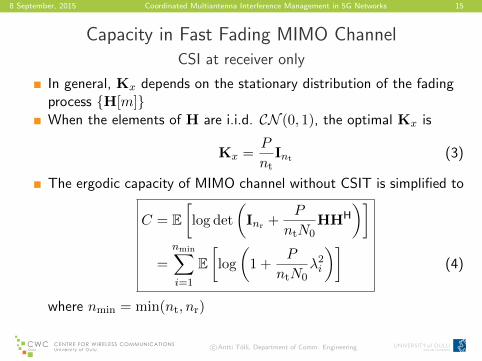
Capacity in Fast Fading MIMO ChannelCSI at receiver only
In general, Kx depends on the stationary distribution of the fadingprocess {H[m]}When the elements of H are i.i.d. CN (0, 1), the optimal Kx is
Kx =P
ntInt (3)
The ergodic capacity of MIMO channel without CSIT is simplified to
C = E[log det
(Inr +
P
ntN0HHH
)]
=
nmin∑
i=1
E[log
(1 +
P
ntN0λ2i
)](4)
where nmin = min(nt, nr)
c©Antti Tolli, Department of Comm. Engineering
8 September, 2015 Coordinated Multiantenna Interference Management in 5G Networks 16
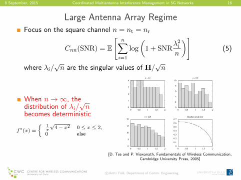
Large Antenna Array RegimeFocus on the square channel n = nt = nr
Cnn(SNR) = E
[n∑
i=1
log
(1 + SNR
λ2in
)](5)
where λi/√n are the singular values of H/
√n
When n→∞, thedistribution of λi/
√n
becomes deterministic
f∗(x) =
{1π
√4− x2 0 ≤ x ≤ 2,
0 else
342 MIMO II: capacity and multiplexing architectures
due to Marcenko and Pastur [78], the empirical distribution of the singularvalues of H/
!n converges to a deterministic limiting distribution for almost
all realizations of H. Figure 8.4 demonstrates the convergence. The limitingdistribution is the so-called quarter circle law.3 The corresponding limitingdensity of the squared singular values is given by
f "!x"=
!"
#
1#
$1x# 1
4 0 $ x $ 4$
0 else%(8.23)
Hence, we can conclude that, for increasing n,
1n
n%
i=1
log&1+ SNR
&2i
n
'%
( 4
0log!1+ SNRx"f "!x"dx% (8.24)
If we denote
c"!SNR" '=( 4
0log!1+ SNRx"f "!x"dx$ (8.25)
Figure 8.4 Convergence of theempirical singular valuedistribution of H/
!n. For
each n, a single randomrealization of H/
!n is
generated and the empiricaldistribution (histogram) of thesingular values is plotted. Wesee that as n grows, thehistogram converges to thequarter circle law.
0 0.5 1 1.5 20
1
2
3
4n = 32
0 0.5 1 1.5 20
2
4
6
8
10n = 64
0 0.5 1 1.5 20
5
10
15
20n = 128
0 0.5 1 1.5 20
0.1
0.2
0.3
0.4
0.5
0.6
0.7Quarter circle law
3 Note that although the singular values are unbounded, in the limit they lie in the interval(0$2) with probability 1.
[D. Tse and P. Viswanath, Fundamentals of Wireless Communication,Cambridge University Press, 2005]
c©Antti Tolli, Department of Comm. Engineering

8 September, 2015 Coordinated Multiantenna Interference Management in 5G Networks 17
Large Antenna Array RegimeFor increasing n 5
1
n
n∑i=1
log
(1 + SNR
λ2i
n
)→∫ 4
0log(1 + SNRx)f∗(x)dx = c∗(SNR) (6)
and the closed form solution to the integral is
c∗(SNR) = 2 log
(1 +√4SNR + 1
2
)−
log e
4SNR
(√4SNR + 1− 1
)2(7)
Furthermore
limn→∞
Cnn(SNR)
n= c∗(SNR)→ Cnn(SNR) ≈ nc∗(SNR) (8)
Capacity grows linearly in n at any SNR5More in: Foundations and Trends in Communications and Information Theory, Vol. 1, Issue 1, ”Random Matrix Theory
and Wireless Communications” by A. Tulino and S Verdu
c©Antti Tolli, Department of Comm. Engineering

8 September, 2015 Coordinated Multiantenna Interference Management in 5G Networks 18
Example: Approximate vs. Exact Capacity
343 8.2 Fast fading MIMO channel
we can solve the integral for the density in (8.23) to arrive at (see Exer-cise 8.17)
c!!SNR"= 2 log!1+ SNR" 1
4F!SNR"
"" log e
4SNRF!SNR"# (8.26)
where
F!SNR" $=##
4SNR+1"1$2
% (8.27)
The significance of c!!SNR" is that
limn$%
Cnn!SNR"n
= c!!SNR"% (8.28)
So capacity grows linearly in n at any SNR and the constant c!!SNR" is therate of the growth.We compare the large-n approximation
Cnn!SNR"& nc!!SNR"# (8.29)
with the actual value of the capacity for n = 2#4 in Figure 8.5. We see theapproximation is very good, even for such small values of n. In Exercise 8.7,we see statistical models other than i.i.d. Rayleigh, which also have a linearincrease in capacity with an increase in n.
Linear scaling: a more in-depth lookTo better understand why the capacity scales linearly with the number ofantennas, it is useful to contrast the MIMO scenario here with three otherscenarios:
Figure 8.5 Comparisonbetween the large-napproximation and the actualcapacity for n= 2! 4.
–5 0 10 15 20SNR (dB)
25 30
Approximate capacity c!
–10
9
8
7
6
5
4
3
2
1
0
Rat
e(b
its /s
/ Hz)
5
Exact capacity 14 C44
Exact capacity 12 C22
Figure: Comparison between the large-n approximation and the actual capacityfor n = 2, 4. [D. Tse and P. Viswanath, Fundamentals of Wireless Communication, Cambridge University Press, 2005]
c©Antti Tolli, Department of Comm. Engineering

8 September, 2015 Coordinated Multiantenna Interference Management in 5G Networks 19
Large Antenna Array Regime, nr >> nt
Assume nr >> nt, and the elements of H are i.i.d. CN (0, 1)
HHH
nr≈ Int (9)
then
log
∣∣∣∣Inr +P
ntN0HHH
∣∣∣∣ = log
∣∣∣∣Int +P
ntN0HHH
∣∣∣∣
≈ nt log(1 +PnrntN0
) (10)
Match filter receiver is asymptotically optimal
c©Antti Tolli, Department of Comm. Engineering

8 September, 2015 Coordinated Multiantenna Interference Management in 5G Networks 20
Large Antenna Array Regime, nt >> nr
Assume nt >> nr, and the elements of H are i.i.d. CN (0, 1)
HHH
nt≈ Inr (11)
then the rate expression without CSIT is simplified to
log
∣∣∣∣Inr +P
ntN0HHH
∣∣∣∣ ≈ nr log(1 +P
N0) (12)
The rate expression with full CSIT (at high SNR) is simplified to
log
∣∣∣∣Inr +1
N0HKxH
H
∣∣∣∣ ≈ nr log(1 +ntnr
P
N0) (13)
The rows of H are asymptotically orthogonal:Kx = VPVH ≈ P
nrntHHH
c©Antti Tolli, Department of Comm. Engineering
8 September, 2015 Coordinated Multiantenna Interference Management in 5G Networks 21
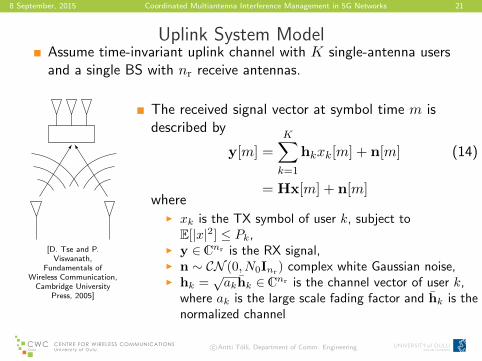
Uplink System ModelAssume time-invariant uplink channel with K single-antenna usersand a single BS with nr receive antennas.
426 MIMO IV: multiuser communication
the downlink. We conclude in Section 10.5 with a discussion of the systemimplications of using MIMO in cellular networks; this will link up the newinsights obtained here with those in Chapters 4 and 6.
10.1 Uplink with multiple receive antennas
We begin with the narrowband time-invariant uplink with each user havinga single transmit antenna and the base-station equipped with an array ofantennas (Figure 10.1). The channels from the users to the base-station aretime-invariant. The baseband model is
y!m"=K!
k=1
hkxk!m"+w!m"# (10.1)
with y!m" being the received vector (of dimension nr , the number of receiveantennas) at time m, and hk the spatial signature of user k impinged on thereceive antenna array at the base-station. User k’s scalar transmit symbol attime m is denoted by xk!m" and w!m" is i.i.d. !" $0#N0Inr% noise.
10.1.1 Space-division multiple access
In the literature, the use of multiple receive antennas in the uplink is oftencalled space-division multiple access (SDMA): we can discriminate amongstthe users by exploiting the fact that different users impinge different spatialsignatures on the receive antenna array.An easy observation we can make is that this uplink is very similar to
the MIMO point-to-point channel in Chapter 5 except that the signals sent
Figure 10.1 The uplink withsingle transmit antenna at eachuser and multiple receiveantennas at the base-station.
out on the transmit antennas cannot be coordinated. We studied preciselysuch a signaling scheme using separate data streams on each of the transmitantennas in Section 8.3. We can form an analogy between users and transmitantennas (so nt , the number of transmit antennas in the MIMO point-to-pointchannel in Section 8.3, is equal to the number of users K). Further, theequivalent MIMO point-to-point channel H is !h1# & & & #hK", constructed fromthe SIMO channels of the users.Thus, the transceiver architecture in Figure 8.1 in conjunction with the
receiver structures in Section 8.3 can be used as an SDMA strategy. Forexample, each of the user’s signal can be demodulated using a linear decorre-lator or an MMSE receiver. The MMSE receiver is the optimal compromisebetween maximizing the signal strength from the user of interest and sup-pressing the interference from the other users. To get better performance, onecan also augment the linear receiver structure with successive cancellationto yield the MMSE–SIC receiver (Figure 10.2). With successive cancella-tion, there is also a further choice of cancellation ordering. By choosing a
[D. Tse and P.Viswanath,
Fundamentals ofWireless Communication,
Cambridge UniversityPress, 2005]
The received signal vector at symbol time m isdescribed by
y[m] =
K∑
k=1
hkxk[m] + n[m]
= Hx[m] + n[m]
(14)
whereI xk is the TX symbol of user k, subject to
E[|x|2] ≤ Pk,I y ∈Cnr is the RX signal,I n ∼ CN (0, N0Inr
) complex white Gaussian noise,I hk =
√akhk ∈Cnr is the channel vector of user k,
where ak is the large scale fading factor and hk is thenormalized channel
c©Antti Tolli, Department of Comm. Engineering
8 September, 2015 Coordinated Multiantenna Interference Management in 5G Networks 22
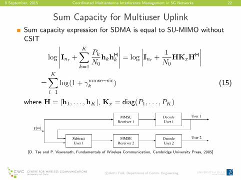
Sum Capacity for Multiuser Uplink
Sum capacity expression for SDMA is equal to SU-MIMO withoutCSIT
log
∣∣∣∣∣Inr +
K∑
k=1
PkN0
hkhHk
∣∣∣∣∣ = log
∣∣∣∣Inr +1
N0HKxH
H
∣∣∣∣
=
K∑
i=1
log(1 + γmmse−sick ) (15)
where H = [h1, . . . ,hK ], Kx = diag(P1, . . . , PK)427 10.1 Uplink with multiple receive antennas
MMSE Receiver 2
MMSE Receiver 1
y[m]
User 2Decode User 2
Subtract User 1
User 1Decode User 1
different order, users are prioritized differently in the sharing of the commonFigure 10.2 The MMSE–SICreceiver: user 1’s data is firstdecoded and then thecorresponding transmit signalis subtracted off before the nextstage. This receiver structure,by changing the ordering ofcancellation, achieves the twocorner points in the capacityregion.
resource of the uplink channel, in the sense that users canceled later are treatedbetter.
Provided that the overall channel matrix H is well-conditioned, all ofthese SDMA schemes can fully exploit the total number of degrees of free-dom min!K"nr# of the uplink channel (although, as we have seen, differentschemes have different power gains). This translates to being able to simul-taneously support multiple users, each with a data rate that is not limitedby interference. Since the users are geographically separated, their trans-mit signals arrive in different directions at the receive array even whenthere is limited scattering in the environment, and the assumption of a well-conditionedH is usually valid. (Recall Example 7.4 in Section 7.2.4.) Contrastthis to the point-to-point case when the transmit antennas are co-located, anda rich scattering environment is needed to provide a well-conditioned channelmatrix H.
Given the power levels of the users, the achieved SINR of each user canbe computed for the different SDMA schemes using the formulas derived inSection 8.3 (Exercise 10.1). Within the class of linear receiver architecture,we can also formulate a power control problem: given target SINR require-ments for the users, how does one optimally choose the powers and linearfilters to meet the requirements? This is similar to the uplink CDMA powercontrol problem described in Section 4.3.1, except that there is a furtherflexibility in the choice of the receive filters as well as the transmit powers.The first observation is that for any choice of transmit powers, one alwayswants to use the MMSE filter for each user, since that choice maximizes theSINR for every user. Second, the power control problem shares the basicmonotonicity property of the CDMA problem: when a user lowers its transmitpower, it creates less interference and benefits all other users in the system.As a consequence, there is a component-wise optimal solution for the pow-ers, where every user is using the minimum possible power to support theSINR requirements. (See Exercise 10.2.) A simple distributed power controlalgorithm will converge to the optimal solution: at each step, each user firstupdates its MMSE filter as a function of the current power levels of the otherusers, and then updates its own transmit power so that its SINR requirementis just met. (See Exercise 10.3.)
[D. Tse and P. Viswanath, Fundamentals of Wireless Communication, Cambridge University Press, 2005]
c©Antti Tolli, Department of Comm. Engineering

8 September, 2015 Coordinated Multiantenna Interference Management in 5G Networks 23
Large Antenna Array Regime, nr >> K
Assume nr >> K, and the elements of hk are i.i.d. CN (0, 1)
HHH
nr≈ AK (16)
where AK = diag(a1, . . . , aK). Then,
∣∣∣∣Inr +1
N0HKxH
H
∣∣∣∣ = log
∣∣∣∣IK +1
N0KxH
HH
∣∣∣∣
≈K∑
k=1
log(1 +nrPkakN0
) (17)
Match filter receiver is asymptotically optimal
c©Antti Tolli, Department of Comm. Engineering

8 September, 2015 Coordinated Multiantenna Interference Management in 5G Networks 24
Downlink System ModelAssume time-invariant downlink channel with K single-antennausers and a single BS with nt transmit antennas.
448 MIMO IV: multiuser communication
10.3 Downlink with multiple transmit antennas
We now turn to the downlink channel, from the base-station to the multiple
Figure 10.15 The downlinkwith multiple transmit antennasat the base-station and singlereceive antenna at each user.
users. This time the base-station has an array of transmit antennas but eachuser has a single receive antenna (Figure 10.15). It is often a practicallyinteresting situation since it is easier to put multiple antennas at the base-station than at the mobile users. As in the uplink case we first consider thetime-invariant scenario where the channel is fixed. The baseband model of thenarrowband downlink with the base-station having nt antennas and K userswith each user having a single receive antenna is
yk!m"= h!kx!m"+wk!m"# k= 1# $ $ $ #K# (10.31)
where yk!m" is the received vector for user k at time m, h!k is an nt dimen-
sional row vector representing the channel from the base-station to user k.Geometrically, user k observes the projection of the transmit signal in thespatial direction hk in additive Gaussian noise. The noise wk!m"" !" %0#N0&and is i.i.d. in time m. An important assumption we are implicitly makinghere is that the channel’s hk are known to the base-station as well as to theusers.
10.3.1 Degrees of freedom in the downlink
If the users could cooperate, then the resulting MIMO point-to- point channelwould have min%nt#K& spatial degrees of freedom, assuming that the rank ofthe matrix H= !h1# $ $ $ #hK" is full. Can we attain this full spatial degrees offreedom even when users cannot cooperate?Let us look at a special case. Suppose h1# $ $ $ #hK are orthogonal (which is
only possible if K # nt). In this case, we can transmit independent streams ofdata to each user, such that the stream for the kth user 'xk!m"( is along thetransmit spatial signature hk, i.e.,
x!m"=K!
k=1
xk!m"hk) (10.32)
The overall channel decomposes into a set of parallel channels; user k receives
yk!m"= $hk$2xk!m"+wk!m") (10.33)
Hence, one can transmit K parallel non-interfering streams of data to theusers, and attain the full number of spatial degrees of freedom in the channel.What happens in general, when the channels of the users are not orthogonal?
Observe that to obtain non-interfering channels for the users in the exampleabove, the key property of the transmit signature hk is that hk is orthogonal
[D. Tse and P.Viswanath,
Fundamentals ofWireless Communication,
Cambridge UniversityPress, 2005]
The received signal vector at symbol time m is
yk[m] = hHk x[m] + wk[m]
= hHkuk√pkdk[m] +
K∑
i=1,i 6=khHkui√pidi[m] + wk[m]
(18)
I x ∈Cnt is the TX signal vector, subject to powerconstraint E[Tr(xxH)] =
∑Kk=1 pk ≤ P ,
I uk ∈Cnt is the normalised beamformer, ‖uk‖ = 1I dk ∈C is the normalised data symbol, E
[|dk|2
]= 1
I yk ∈C is the RX signal,I wk ∼ CN (0, N0) complex white Gaussian noise,I hk =
√akhk ∈Cnt is the channel vector of user k
assumed to be ideally known at the transmitter
c©Antti Tolli, Department of Comm. Engineering
8 September, 2015 Coordinated Multiantenna Interference Management in 5G Networks 25
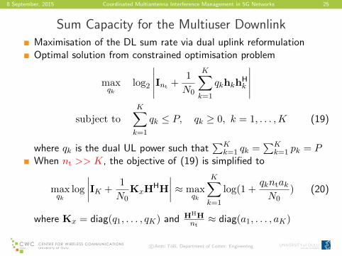
Sum Capacity for the Multiuser DownlinkMaximisation of the DL sum rate via dual uplink reformulationOptimal solution from constrained optimisation problem
maxqk
log2
∣∣∣∣∣Int +1
N0
K∑
k=1
qkhkhHk
∣∣∣∣∣
subject to
K∑
k=1
qk ≤ P, qk ≥ 0, k = 1, . . . ,K (19)
where qk is the dual UL power such that∑K
k=1 qk =∑K
k=1 pk = PWhen nt >> K, the objective of (19) is simplified to
maxqk
log
∣∣∣∣IK +1
N0KxH
HH
∣∣∣∣ ≈ maxqk
K∑
k=1
log(1 +qkntakN0
) (20)
where Kx = diag(q1, . . . , qK) and HHHnt≈ diag(a1, . . . , aK)
c©Antti Tolli, Department of Comm. Engineering

8 September, 2015 Coordinated Multiantenna Interference Management in 5G Networks 26
Linear MMSE Receiver – DerivationConsider the uplink system model y[m] = Hx[m] + n[m] (41),where the decision variables are generated as x = WHyAssume n ∼ CN (0,Kn) and x ∼ CN (0,Kx) are independent, theoptimal linear MMSE receiver is found by minimizing
W = arg minW
E[‖x−WHy‖2
]
︸ ︷︷ ︸MSE
(21)
After differentiation with respect to W and setting the gradient tozero, the optimal MMSE filter is
W =(HKxHH + Kn
)−1HKx (22)
If n ∼ CN (0, N0Inr) and x ∼ CN (0, PntInt)
W =
(P
ntHHH +N0I
)−1HP
nt(23)
c©Antti Tolli, Department of Comm. Engineering

8 September, 2015 Coordinated Multiantenna Interference Management in 5G Networks 27
Linear MMSE Receiver – SINR Derivation
Low SNR: P << N0 → W ≈ H Pnt
= Matched filter
High SNR: P >> N0 → W ≈(HHH
)−1H = ZF receiver
Output SINR for the kth stream with input power pk (P/nt) is
γmmsek =
E[|wH
k hkxk|2]
E[|wH
k (∑
i 6=k hixi + nk)|2] =
pkwHk hkh
Hkwk
wHkRkwk
= . . .
= pkhHkR−1k hk (24)
where Rk =∑
i 6=k pihihHi +N0Inr and wk is kth column of W
Achievable rate:
Rmmse = E
[nt∑
k=1
log(1 + γmmsek )
](25)
c©Antti Tolli, Department of Comm. Engineering

8 September, 2015 Coordinated Multiantenna Interference Management in 5G Networks 28
Large System Approximation of γmmsek
Some important lemmas
Lemma 1: Assume a vector x ∈ CN with i.i.d elements which havezero mean and variance equal to 1
N . Also consider a Hermitianmatrix A ∈ CN×N with elements independent of x, then
xHAx− 1
Ntr(A)
N→∞−−−−→ 0 (26)
Lemma 2:Let AN be a complex N ×N matrix with uniformlybounded spectral norm. Also, consider random Hermitian matrixCN such that for smallest eigenvalue of CN there exist an ε withprobability one such that λmin > ε for all large N , then
1
Ntr[ANC−1N ]− 1
Ntr[AN (CN + uuH)−1]
N→∞−−−−→ 0 (27)
where u is a complex vector.
c©Antti Tolli, Department of Comm. Engineering

8 September, 2015 Coordinated Multiantenna Interference Management in 5G Networks 29
Large System Approximation of γmmsek
Theorem 3: Stieltjes transform of Gram matrix YYH. Consider aN × n random matrix denoted by Y, such that elements of Y areindependent and zero mean. The variance of entries is given byE[|yi,j |2] = α2
i,j
mYYH(z) =
1
Ntr(YYH − zIN)−1 − 1
Ntr(Θ(z))
n→∞, Nn→ c−−−−−−−−→ 0
(28)where Θ(z) = diag(θ1(z), ..., θN (z)). The entries θi can be foundby fixed point iteration
θi(z) =−1
z(1 + 1n
n∑j=1
α2i,j θj(z))
∀1 ≤ i ≤ N (29)
θj(z) =−1
z(1 + 1n
N∑i=1
α2i,jθi(z))
∀1 ≤ j ≤ n (30)
c©Antti Tolli, Department of Comm. Engineering

8 September, 2015 Coordinated Multiantenna Interference Management in 5G Networks 30
Large System Approximation of γmmsek
The instantaneous random variable γmmsek (p) can be approximated
by a deterministic quantity γdetk (p) such that
γmmsek (p)− γdetk (p)
nr →∞, nrK→ c−−−−−−−−−→ 0 (31)
Sketch of proofI Define Σk =
∑i 6=k pihih
Hi and Σ = Hdiag(p1, . . . , pK)HH
I Applying Lemma 1, γmmsek can be approximated as
pkakhHk (Σk +N0Inr
)−1
hk →pkaknr
Tr(
(Σk +N0Inr)−1)
(32)
I Applying Lemma 2, we have
pkaknr
Tr(
(Σk +N0Inr)−1)≈ pkak
nrTr(
(Σ +N0Inr)−1)
= pkakmΣ(−N0) (33)
where mΣ(−N0) is the Stieltjes transform of Σ and it only dependson p and a1, . . . , ak
c©Antti Tolli, Department of Comm. Engineering

8 September, 2015 Coordinated Multiantenna Interference Management in 5G Networks 31
Large System Approximation of γmmsek
Uplink with K single-antenna users and a single BS with nr receiveantennas.
Number of users
48 16 32 64 128 256
Va
r(γ
mm
se
- γ
de
t)
0
1
2
3
4
5
6
7
8
9
Figure: Variance of γmmsek − γdetk , K = nr and pkak/N0 = 10
c©Antti Tolli, Department of Comm. Engineering

8 September, 2015 Coordinated Multiantenna Interference Management in 5G Networks 32
OutlineEvolution of multiantenna systemsMIMO with large antenna arraysLinear transceiver design and resource allocation
I Introduction to convex optimisationI Resource allocation and linear transceiver designI Coordinated transceiver optimisationI Coherent vs. coordinated beamforming
Minimum power multicell beamforming with QoS constraintsI Centralised solutionI Decentralised solution via optimisation decompositionI Large system approximation
Throughput optimal linear TX-RX designI Weighted sum rate maximisation (WSRM) via MSE minimisationI WSRM with rate constraintsI Decentralised solution via precoded UL pilotI Bidirectional signalling strategies for dynamic TDDI Mode selection and transceiver design in underlay D2D MIMO
systemsc©Antti Tolli, Department of Comm. Engineering

8 September, 2015 Coordinated Multiantenna Interference Management in 5G Networks 33
Constrained Optimisation Problem
Engineering designs are often posed as constrained optimisationproblems:
minimise f0(x)subject to fi(x) ≤ 0, i = 1, . . . ,m
hi(x) = 0, i = 1, . . . , p(34)
whereI x is a vector of decision variablesI f0 is the objective functionI fi(x), i = 1, . . . ,m are the inequality constraint functionsI hi(x), i = 1, . . . , p are the equality constraint functions
Hard to solve in generalI especially when the number of variables in x is largeI the problem might have multiple local minimaI difficult to find a feasible solutionI possibly poor convergence rate
c©Antti Tolli, Department of Comm. Engineering

8 September, 2015 Coordinated Multiantenna Interference Management in 5G Networks 34
Convex Optimisation ProblemIf f0, f1, . . . , fm in
minimise f0(x)subject to fi(x) ≤ 0, i = 1, . . . ,m
hi(x) = 0, i = 1, . . . , p(35)
are convex and hi, i = 1, . . . , p are affine (hi(x) = aTi x− bi), then
I any locally optimal point is globally optimalI feasibility can be determined unambiguouslyI can be solved efficiently using, e.g. interior point methods
incorporated in generic convex optimisation tools
A function f is convex if its domain dom(f) is convex andf(θx+ (1− θ)y) ≤ θf(x) + (1− θ)f(y) ∀ x, y ∈ dom(f), θ ∈ [0, 1]
then so are the sets
f!1(S) = {x | Ax + b ! S}f(T ) = {Ax + b | x ! T }
An example is coordinate projection {x | (x, y) !S for some y}. As another example, a constraint of theform
"Ax + b"2 # cT x + d,
where A ! Rk"n, a second-order cone constraint, sinceit is the same as requiring the affine expression (Ax +b, cT x + d) to lie in the second-order cone in Rk+1.Similarly, if A0, A1, . . . , Am ! Sn, solution set of thelinear matrix inequality (LMI)
F (x) = A0 + x1A1 + · · · + xmAm $ 0
is convex (preimage of the semidefinite cone under anaffine function).A linear-fractional (or projective) function f : Rm %
Rn has the form
f(x) =Ax + b
cT x + d
and domain dom f = H = {x | cT x + d > 0}. If Cis a convex set, then its linear-fractional transformationf(C) is also convex. This is because linear fractionaltransformations preserve line segments: for x, y ! H,
f([x, y]) = [f(x), f(y)]
PSfrag replacementsx1 x2
x3x4
PSfrag replacementsf(x1) f(x2)
f(x3)f(x4)
Two further properties are helpful in visualizing thegeometry of convex sets. The first is the separatinghyperplane theorem, which states that if S, T & Rn
are convex and disjoint (S ' T = (), then there exists ahyperplane {x | aT x ) b = 0} which separates them.
PSfrag replacements ST
a
The second property is the supporting hyperplane the-orem which states that there exists a supporting hy-perplane at every point on the boundary of a convex
set, where a supporting hyperplane {x | aT x = aT x0}supports S at x0 ! !S if
x ! S * aT x # aT x0
PSfrag replacementsS
x0
a
III. CONVEX FUNCTIONS
In this section, we introduce the reader to someimportant convex functions and techniques for verifyingconvexity. The objective is to sharpen the reader’s abilityto recognize convexity.
A. Convex functionsA function f : Rn % R is convex if its domain dom f
is convex and for all x, y ! dom f , " ! [0, 1]
f("x + (1 ) ")y) # "f(x) + (1 ) ")f(y);
f is concave if )f is convex.PSfrag replacements
xxx
convex concave neither
Here are some simple examples on R: x2 is convex(dom f = R); log x is concave (dom f = R++); andf(x) = 1/x is convex (dom f = R++).It is convenient to define the extension of a convex
function f
f(x) =
!f(x) x ! dom f++ x ,! dom f
Note that f still satisfies the basic definition for allx, y ! Rn, 0 # " # 1 (as an inequality in R - {++}).We will use the same symbol for f and its extension,i.e., we will implicitly assume convex functions areextended.The epigraph of a function f is
epi f = {(x, t) | x ! dom f, f(x) # t }
PSfrag replacements
x
f(x)
epi f
5
c©Antti Tolli, Department of Comm. Engineering

8 September, 2015 Coordinated Multiantenna Interference Management in 5G Networks 35
A Simple Exampleinfeasible). A point x ! C is an optimal point if f(x) =f! and the optimal set is Xopt = {x ! C | f(x) = f!}.As an example consider the problem
minimize x1 + x2
subject to "x1 # 0"x2 # 01 " $
x1x2 # 0
0 1 2 3 4 50
1
2
3
4
5
PSfrag replacements
x1
x2
CCC
The objective function is f0(x) = [1 1]T x; the feasibleset C is half-hyperboloid; the optimal value is f ! = 2;and the only optimal point is x! = (1, 1).In the standard problem above, the explicit constraints
are given by fi(x) # 0, hi(x) = 0. However, there arealso the implicit constraints: x ! dom fi, x ! domhi,i.e., x must lie in the set
D = dom f0 % · · ·%dom fm %domh1 % · · ·%domhp
which is called the domain of the problem. For example,
minimize " log x1 " log x2
subject to x1 + x2 " 1 # 0
has the implicit constraint x ! D = {x ! R2 | x1 >0, x2 > 0}.A feasibility problem is a special case of the standard
problem, where we are interested merely in finding anyfeasible point. Thus, problem is really to
• either find x ! C• or determine that C = & .
Equivalently, the feasibility problem requires that weeither solve the inequality / equality system
fi(x) # 0, i = 1, . . . , mhi(x) = 0, i = 1, . . . , p
or determine that it is inconsistent.An optimization problem in standard form is a convex
optimization problem if f0, f1, . . . , fm are all convex,and hi are all affine:
minimize f0(x)subject to fi(x) # 0, i = 1, . . . , m
aTi x " bi = 0, i = 1, . . . , p.
This is often written asminimize f0(x)subject to fi(x) # 0, i = 1, . . . , m
Ax = b
where A ! Rp!n and b ! Rp. As mentioned in theintroduction, convex optimization problems have threecrucial properties that makes them fundamentally moretractable than generic nonconvex optimization problems:
1) no local minima: any local optimum is necessarilya global optimum;
2) exact infeasibility detection: using duality theory(which is not cover here), hence algorithms areeasy to initialize;
3) efficient numerical solution methods that can han-dle very large problems.
Note that often seemingly ‘slight’ modifications ofconvex problem can be very hard. Examples include:
• convex maximization, concave minimization, e.g.
maximize 'x'subject to Ax ( b
• nonlinear equality constraints, e.g.
minimize cT xsubject to xT Pix + qT
i x + ri = 0, i = 1, . . . , K
• minimizing over non-convex sets, e.g., Booleanvariables
find xsuch that Ax ( b,
xi ! {0, 1}
To understand global optimality in convex problems,recall that x ! C is locally optimal if it satisfies
y ! C, 'y " x' # R =) f0(y) * f0(x)
for some R > 0. A point x ! C is globally optimalmeans that
y ! C =) f0(y) * f0(x).
For convex optimization problems, any local solution isalso global. [Proof sketch: Suppose x is locally optimal,but that there is a y ! C, with f0(y) < f0(x). Thenwe may take small step from x towards y, i.e., z =!y +(1"!)x with ! > 0 small. Then z is near x, withf0(z) < f0(x) which contradicts local optimality.]There is also a first order condition that characterizes
optimality in convex optimization problems. Suppose f0
is differentiable, then x ! C is optimal iff
y ! C =) +f0(x)T (y " x) * 0
So "+f0(x) defines supporting hyperplane for C at x.This means that if we move from x towards any otherfeasible y, f0 does not decrease.
9
x1[A. Hindi, ”A Tutorial on Convex Optimization”, Proc. of the 2004 American Control Conference Boston, Massachusetts,June, 2004]
c©Antti Tolli, Department of Comm. Engineering

8 September, 2015 Coordinated Multiantenna Interference Management in 5G Networks 36
Resource Allocation with MIMO
Multiuser MIMO: base station and users are equipped with multipleantennas
I The fundamental idea: inter-user interference is minimised
I Requires channel knowledge of all same cell users
Multiple users – only a subset of users selected at a timeI Scheduling/resource allocation
In general, a difficult non-convex combinatorial problem
1. Select a set of users for each orthogonal dimension(frequency/sub-carrier, time)
2. Optimise transceivers for the selected set of users per dimension.
Greedy allocation: Select a set of users with best channel conditionssuch that their spatial signatures overlap as little as possible
I Often unfair, users with weak channel conditions suffer
c©Antti Tolli, Department of Comm. Engineering

8 September, 2015 Coordinated Multiantenna Interference Management in 5G Networks 37
Resource Allocation with MIMO
User 1
User 2
User 3
User 4
MIMOBS
Time instant t
User 1
User 2
User 3
User 4
MIMOBS
Time instant t+1
c©Antti Tolli, Department of Comm. Engineering

8 September, 2015 Coordinated Multiantenna Interference Management in 5G Networks 38
Multi-cell MIMO System ModelB BSs, NT TX antennas per BS and NRk RX antennas per user kA user k is served by Mk = |Bk| BSs from the joint processing setBk, Bk ⊆ B = {1, . . . , B}6
yk =∑
b∈Bab,kHb,kx
′b + nk (36)
=∑
b∈Bk
ab,kHb,kxb,k +∑
b∈Bk
ab,kHb,k
∑
i6=kxb,i
+∑
b∈B\Bk
ab,kHb,kx′b + nk
whereI ab,kHb,k ∈CNRk
×NT channel from BS b to user k
I x′b ∈CNT total TX signal from BS b, and
I xb,k is the transmitted data vector from BS b to user k6Extension to multicarrier systems is straightforward – add sub-carrier index c to every variable
c©Antti Tolli, Department of Comm. Engineering

8 September, 2015 Coordinated Multiantenna Interference Management in 5G Networks 39
System Model
xb,k = Mb,kdk ∈CNT is the transmitted data vector from BS b touser k, where
I Mb,k ∈CNT×mk pre-coding matrix,
I dk = [d1,k, . . . , dmk,k]T vector of normalised data symbols,
I mk ≤ min(NTMk, NRk) number of active data streams.
The optimal linear receiver is equipped with a LMMSE filter,
dk = UHk yk:
Uk =
(K∑
i=1
∑
b∈Bi
a2b,kHb,kMb,iMHb,iH
Hb,k +N0INRk
)−1
∑
b∈Bk
ab,kHb,kMb,k (37)
c©Antti Tolli, Department of Comm. Engineering

8 September, 2015 Coordinated Multiantenna Interference Management in 5G Networks 40
Linear Transceiver DesignEntire capacity region of multiuser MIMO DL has been recentlydiscovered
I Also with individual peak power constraint per BS antenna78
I Require complex nonlinear precoding based on dirty paper coding
I Sub-optimal but less complex transmission methods are neededLinear beamforming is usually remarkably simpler in practice
I Dimensionality contraint per BS:
0 ≤∑
k∈Ubmk ≤ NT, 0 ≤ mk ≤ NRk
. (38)
I Dimensionality constraint in the multi-cell network: Upper bound∑k∈U mk ≤ BNT
I Very difficult in general (feasibility conditions for interferencealignment in high SNR)
7W. Yu and T. Lan, ”Transmitter optimization for the multi-antenna downlink with per-antenna power constraints,” IEEETransactions on Signal Processing, vol. 55, no. 6, part 1, pp. 2646–2660, Jun. 2007.
8H. Weingarten, Y. Steinberg, and S. Shamai, ”The capacity region of the Gaussian multiple-input multiple-outputbroadcast channel,” IEEE Transactions on Information Theory, vol. 52, no. 9, pp. 3936–3964, Sep. 2006.
c©Antti Tolli, Department of Comm. Engineering

8 September, 2015 Coordinated Multiantenna Interference Management in 5G Networks 41
Linear Transceiver DesignA generalised method for joint design of linear transceivers with
I Coordinated multi-cell processing
I Per-BS or per-antenna power constraints
I Subject to various optimisation criteria and Quality of Service (QoS)constraints
The proposed method can accommodate any scenario betweenI Coherent multi-cell beamforming across virtual MIMO channel
I Single-cell beamforming with inter-cell interference coordination andbeam allocation
The presented methods require a complete CSI between all pairs ofusers and BSs
I The solution represent an upper bound for the less ideal solutionswith an incomplete CSI.
Centralised and decentralised mechanisms to perform scheduling andprecoding
c©Antti Tolli, Department of Comm. Engineering

8 September, 2015 Coordinated Multiantenna Interference Management in 5G Networks 42
Linear Transceiver Design
Per data stream processing: B BSs send S independent streams,S ≤ min(BNT,
∑k∈U NRk)
For each data stream s, scheduler associates a user ks, with thechannel matrices Hb,ks , b ∈ Bs.
I In some special cases Bs ⊆ Bks . For example, a user may receive datafrom several BSs, while |Bs| = 1 ∀ s.
Let mb,s ∈CNT and us ∈CNRks be arbitrary TX and RX
beamformers for the stream s
SINR per stream:
γs =
∣∣ ∑b∈Bs
ab,ksuHs Hb,ksmb,se
jφb∣∣2
N0
∥∥us∥∥22
+S∑
i=1,i 6=s
∣∣ ∑b∈Bi
ab,ksuHs Hb,ksmb,iejφb
∣∣2(39)
φb represents the possible carrier phase uncertainty of BS b
c©Antti Tolli, Department of Comm. Engineering

8 September, 2015 Coordinated Multiantenna Interference Management in 5G Networks 43
Coordinated Transceiver Optimisation
The SINR expression can accommodate several special cases formulticell coordination:
1. Coherent multi-cell beamforming (Bs = Bk = B ∀ s, k) with per BSand/or per-antenna power constraints
2. Coordinated single-cell beamforming (|Bs| = 1 ∀ s): the other-celltransmissions considered as inter-cell interference
3. Any combination of above two, where |Bk| and |Bs| may be differentfor each user k and/or stream s.
γs =
∣∣ ∑b∈Bs
ab,ksuHs Hb,ksmb,se
jφb∣∣2
N0
∥∥us∥∥22
+S∑
i=1,i 6=s
∣∣ ∑b∈Bi
ab,ksuHs Hb,ksmb,iejφb
∣∣2
c©Antti Tolli, Department of Comm. Engineering

8 September, 2015 Coordinated Multiantenna Interference Management in 5G Networks 44
Coordinated Transceiver Optimisation
The general system optimisation objective is to maximise a functionf(γ1, . . . , γS) that depends on the individual SINR values
maximise f(γ1, . . . , γS)
subject to
∣∣ ∑b∈Bs
ab,ksuHs Hb,ksmb,s
∣∣2
N0
∥∥us∥∥22
+S∑
i=1,i 6=s
∣∣ ∑b∈Bi
ab,ksuHs Hb,ksmb,i
∣∣2≥ γs,
s = 1, . . . , S∑s∈Sb
∥∥mb,s
∥∥22≤ Pb, b = 1, . . . , B
(40)
Additional Quality of Service constraints (QoS) can be alsoincorporated in (40), e.g., minimum/maximum SINR or rateconstraints per stream or per user
c©Antti Tolli, Department of Comm. Engineering

8 September, 2015 Coordinated Multiantenna Interference Management in 5G Networks 45
Coordinated Transceiver Optimisation
Optimisation criteria, e.g.,
1. Sum power minimisation with fixed per stream SINR constraints:f(γ1, . . . , γS) = −∑B
b=1 Pb
2. Weighted sum MSE minimisation:f(γ1, . . . , γS) = −∑S
s=1 βsMSEs = −∑Ss=1
βs
(1+γs)
3. Weighted sum rate maximisation:f(γ1, . . . , γS) =
∑Ss=1 βs log2(1 + γs) = log2
∏Ss=1(1 + γs)
βs
4. Max min weighted SINR per data stream, i.e., SINR balancing :f(γ1, . . . , γS) = max mins=1,...,S β
−1s γs
5. Maximisation of weighted common user rate:f(γ1, . . . , γS) = ro = mink∈A β
−1k
∑s∈Pk
log2 (1 + γs),Pk is a subset of data streams that correspond to user k
c©Antti Tolli, Department of Comm. Engineering

8 September, 2015 Coordinated Multiantenna Interference Management in 5G Networks 46
Coordinated Transceiver Optimisation
Linear MIMO transceiver optimisation problems cannot be solveddirectly, in general – iterative procedures are required
I No cooperation between usersI Transmitter and receivers optimised separately in an iterative mannerI Some controlled inter-user interference allowed
Transmit beamformers
optimised
Iteration t+1
Controller
Receive
beamformers
fixed
c©Antti Tolli, Department of Comm. Engineering

8 September, 2015 Coordinated Multiantenna Interference Management in 5G Networks 47
Coherent Multi-cell versus Coordinated Single-cellBeamforming
A. Tolli, H. Pennanen and P. Komulainen, ”On the Value of Coherent and CoordinatedMulti-cell Transmission”, The International Workshop on LTE Evolution in conjunctionwith the International Conference on Communications (ICC’09), Dresden, Germany,June 2009
A. Tolli, M. Codreanu, and M. Juntti, ”Linear multiuser MIMO transceiver design withquality of service and per antenna power constraints,” IEEE Transactions on SignalProcessing, vol. 56, no. 7, pp. 3049 – 3055, Jul. 2008.
A. Tolli, M. Codreanu, and M. Juntti, ”Cooperative MIMO-OFDM cellular system withsoft handover between distributed base station antennas,” IEEE Transactions onWireless Communications, vol. 7, no. 4, pp. 1428–1440, Apr. 2008.
c©Antti Tolli, Department of Comm. Engineering

8 September, 2015 Coordinated Multiantenna Interference Management in 5G Networks 48
Coordinated single-cell beamformingEach stream is transmitted from a single BS, |Bs| = 1 ∀ sA user ks is typically allocated to arg max
b∈Bab,ks
Near the cell edge, the optimal beam allocation strategy depends onthe the channel Hb,k.
Large gains from fast beam allocation (cell selection) availableI A difficult combinatorial problem → exhaustive searchI Sub-optimal allocation algorithms
Allocation objectives
I Generate the least inter-streaminterference
I Provide large beamforming gainsController
c©Antti Tolli, Department of Comm. Engineering

8 September, 2015 Coordinated Multiantenna Interference Management in 5G Networks 49
Heuristic Beam Allocation Algorithms
1. Greedy selection: Beams with the largest component orthogonal tothe previously selected set of beams are chosen.
2. Maximum eigenvalue selection: The eigenvalues of channel vectorsare simply sorted and at most NT streams are allocated per cell.
3. Eigenbeam selection using maxmin SINR criterion:
I A simplified exhaustive search over all possible combinations ofuser-to-cell and stream/beam-to-user allocations
I Beamformers matched to the channel, i.e., mb,s = vb,ks,ls√PT/|Sb|
I For each allocation, the receivers us and the corresponding SINRvalues γs are recalculated
I The selection of the allocation is based on the maxmin SINRcriterion, i.e., arg max
b,k,lmin
s=1,...,Sγs.
c©Antti Tolli, Department of Comm. Engineering

8 September, 2015 Coordinated Multiantenna Interference Management in 5G Networks 50
Simulation Cases
1. Coherent multi-cell MIMO transmission (Bs = B ∀ s) with per BSpower constraints
2. Coordinated single-cell transmission (|Bs| = 1 ∀ s)I Exhaustive search over all possible combinations of beam allocations.
The SINR balancing algorithm is recomputed for each allocation.
I Fixed allocation, i.e., user ks is always allocated to a cell b with thesmallest path loss, arg max
b∈Bab,ks .
I Heuristic allocation methods
3. Non-coordinated single-cell transmission (|Bs| = 1 ∀ s), where theinter-cell interference is neglected at the transmitters
4. Single-cell transmission with time-division multiple access (TDMA),i.e., without inter-cell interference
c©Antti Tolli, Department of Comm. Engineering
8 September, 2015 Coordinated Multiantenna Interference Management in 5G Networks 51
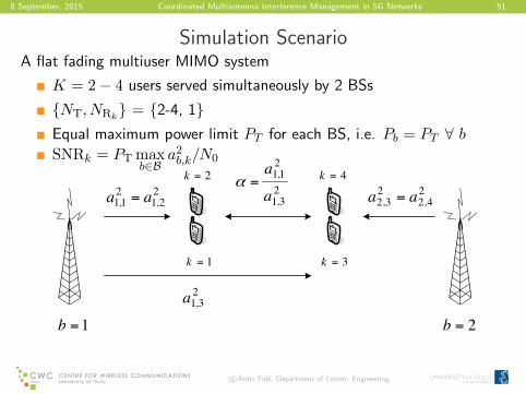
Simulation ScenarioA flat fading multiuser MIMO system
K = 2− 4 users served simultaneously by 2 BSs
{NT, NRk} = {2-4, 1}Equal maximum power limit PT for each BS, i.e. Pb = PT ∀ bSNRk = PT max
b∈Ba2b,k/N0
1=k
1=b 2=b
22,1
21,1 aa = 2
4,223,2 aa =
3=k
23,1a
23,1
21,1
a
a=α2=k 4=k
c©Antti Tolli, Department of Comm. Engineering
8 September, 2015 Coordinated Multiantenna Interference Management in 5G Networks 52
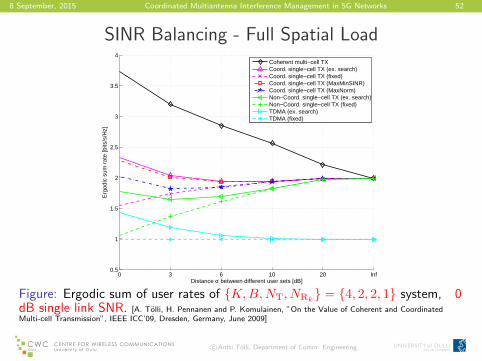
SINR Balancing - Full Spatial Load
0 3 6 10 20 Inf0.5
1
1.5
2
2.5
3
3.5
4
Distance α between different user sets [dB]
Erg
odic
sum
rat
e [b
its/s
/Hz]
Coherent multi−cell TXCoord. single−cell TX (ex. search)Coord. single−cell TX (fixed)Coord. single−cell TX (MaxMinSINR)Coord. single−cell TX (MaxNorm)Non−Coord. single−cell TX (ex. search)Non−Coord. single−cell TX (fixed)TDMA (ex. search)TDMA (fixed)
Figure: Ergodic sum of user rates of {K,B,NT, NRk} = {4, 2, 2, 1} system, 0
dB single link SNR. [A. Tolli, H. Pennanen and P. Komulainen, ”On the Value of Coherent and CoordinatedMulti-cell Transmission”, IEEE ICC’09, Dresden, Germany, June 2009]
c©Antti Tolli, Department of Comm. Engineering

8 September, 2015 Coordinated Multiantenna Interference Management in 5G Networks 53
SINR Balancing - Full Spatial Load
0 3 6 10 20 Inf0
2
4
6
8
10
12
14
16
18
20
Distance α between different user sets [dB]
Erg
odic
sum
rat
e [b
its/s
/Hz]
Coherent multi−cell TXCoord. single−cell TX (ex. search)Coord. single−cell TX (fixed)Coord. single−cell TX (MaxMinSINR)Coord. single−cell TX (MaxNorm)Non−Coord. single−cell TX (ex. search)Non−Coord. single−cell TX (fixed)TDMA (ex. search)TDMA (fixed)
Figure: Ergodic sum of user rates of {K,B,NT, NRk} = {4, 2, 2, 1} system, 20
dB single link SNR. [A. Tolli, H. Pennanen and P. Komulainen, ”On the Value of Coherent and CoordinatedMulti-cell Transmission”, IEEE ICC’09, Dresden, Germany, June 2009]
c©Antti Tolli, Department of Comm. Engineering

8 September, 2015 Coordinated Multiantenna Interference Management in 5G Networks 54
SINR Balancing - Partial Spatial Load
0 3 6 10 20 Inf2
4
6
8
10
12
14
16
Distance α between different user sets [dB]
Erg
odic
sum
rat
e [b
its/s
/Hz]
Coherent multi−cell TXCoord. single−cell TX (ex. search)Coord. single−cell TX (fixed)Coord. single−cell TX (MaxMinSINR)Coord. single−cell TX (MaxNorm)Coordinated single−cell TX (Greedy)Non−Coord. single−cell TX (ex. search)Non−Coord. single−cell TX (fixed)TDMA (ex. search)TDMA (fixed)
Figure: Ergodic sum rate of {K,B,NT, NRk} = {2, 2, 2, 1} system at 20 dB
single link SNR. [A. Tolli, H. Pennanen and P. Komulainen, ”On the Value of Coherent and Coordinated Multi-cellTransmission”, IEEE ICC’09, Dresden, Germany, June 2009]
c©Antti Tolli, Department of Comm. Engineering
8 September, 2015 Coordinated Multiantenna Interference Management in 5G Networks 55
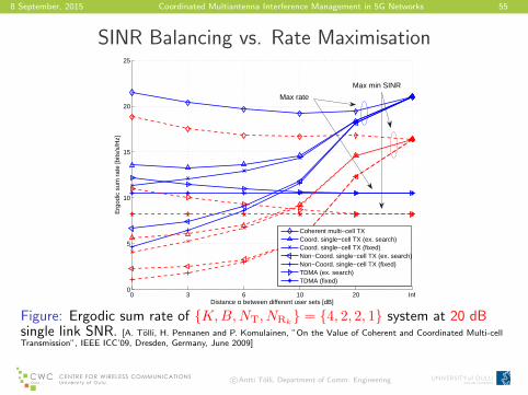
SINR Balancing vs. Rate Maximisation
0 3 6 10 20 Inf0
5
10
15
20
25
Distance α between different user sets [dB]
Erg
odic
sum
rat
e [b
its/s
/Hz]
Max rate
Max min SINR
Coherent multi−cell TXCoord. single−cell TX (ex. search)Coord. single−cell TX (fixed)Non−Coord. single−cell TX (ex. search)Non−Coord. single−cell TX (fixed)TDMA (ex. search)TDMA (fixed)
Figure: Ergodic sum rate of {K,B,NT, NRk} = {4, 2, 2, 1} system at 20 dB
single link SNR. [A. Tolli, H. Pennanen and P. Komulainen, ”On the Value of Coherent and Coordinated Multi-cellTransmission”, IEEE ICC’09, Dresden, Germany, June 2009]
c©Antti Tolli, Department of Comm. Engineering

8 September, 2015 Coordinated Multiantenna Interference Management in 5G Networks 56
OutlineEvolution of multiantenna systemsMIMO with large antenna arraysLinear transceiver design and resource allocation
I Introduction to convex optimisationI Resource allocation and linear transceiver designI Coordinated transceiver optimisationI Coherent vs. coordinated beamforming
Minimum power multicell beamforming with QoS constraintsI Centralised solutionI Decentralised solution via optimisation decompositionI Large system approximation
Throughput optimal linear TX-RX designI Weighted sum rate maximisation (WSRM) via MSE minimisationI WSRM with rate constraintsI Decentralised solution via precoded UL pilotI Bidirectional signalling strategies for dynamic TDDI Mode selection and transceiver design in underlay D2D MIMO
systemsc©Antti Tolli, Department of Comm. Engineering

8 September, 2015 Coordinated Multiantenna Interference Management in 5G Networks 57
Minimum Power Multi-cell Beamforming with UserSpecific QoS Constraints
D. N. C. Tse and P. Viswanath, Fundamentals of Wireless Communication. CambridgeUniversity Press, 2005, Chapter 10
H. Dahrouj and W. Yu, ”Coordinated beamforming for the multicell multi-antennawireless system”, IEEE Transactions on Wireless Communications, vol. 9, no. 5, pp.1748–1759, 2010.
A. Tolli, H. Pennanen, and P. Komulainen, ”Decentralized Minimum Power Multi-cellBeamforming with Limited Backhaul Signalling”, IEEE Trans. on Wireless Comm., vol.10, no. 2, pp. 570 - 580, February 2011
H. Pennanen, A. Tolli and M. Latva-aho, ”Decentralized Coordinated DownlinkBeamforming via Primal Decomposition”, IEEE Signal Processing Letters, vol. 8, no.11,pp. 647 - 650, November 2011
H. Pennanen, A. Tolli and M. Latva-aho, ”Multi-Cell Beamforming with DecentralizedCoordination in Cognitive and Cellular Networks”, IEEE Transactions on SignalProcessing, vol. 62, no. 2, pp. 295 - 308, January 2014
c©Antti Tolli, Department of Comm. Engineering
8 September, 2015 Coordinated Multiantenna Interference Management in 5G Networks 58
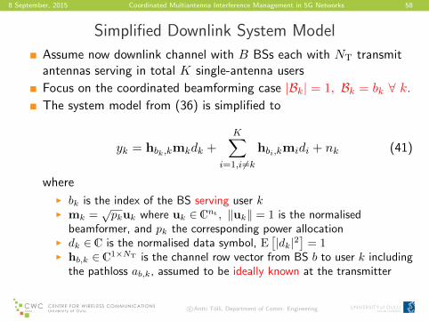
Simplified Downlink System Model
Assume now downlink channel with B BSs each with NT transmitantennas serving in total K single-antenna users
Focus on the coordinated beamforming case |Bk| = 1, Bk = bk ∀ k.
The system model from (36) is simplified to
yk = hbk,kmkdk +
K∑
i=1,i 6=khbi,kmidi + nk (41)
whereI bk is the index of the BS serving user kI mk =
√pkuk where uk ∈Cnt , ‖uk‖ = 1 is the normalised
beamformer, and pk the corresponding power allocationI dk ∈C is the normalised data symbol, E
[|dk|2
]= 1
I hb,k ∈C1×NT is the channel row vector from BS b to user k includingthe pathloss ab,k, assumed to be ideally known at the transmitter
c©Antti Tolli, Department of Comm. Engineering

8 September, 2015 Coordinated Multiantenna Interference Management in 5G Networks 59
Coordinated Minimum Power Beamforming
Minimise the transmitted power
Subject to user specific SINRtargets
Controller Centralised optimisation problem:
min.NB∑b=1
∑k∈Ub
∥∥mk
∥∥22
s. t.
∣∣hbk,kmk
∣∣2
N0 +K∑
i=1,i 6=k
∣∣hbi,kmi
∣∣2≥ γtargetk , k = 1, . . . K
(42)
where the variables are mk ∈CNT , k = 1, . . . ,K.
c©Antti Tolli, Department of Comm. Engineering
8 September, 2015 Coordinated Multiantenna Interference Management in 5G Networks 60
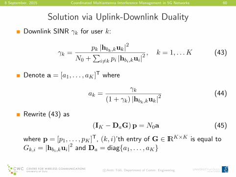
Solution via Uplink-Downlink Duality
Downlink SINR γk for user k:
γk =pk |hbk,kuk|2
N0 +∑
i 6=k pi |hbi,kui|2, k = 1, . . .K (43)
Denote a = [a1, . . . , aK ]T where
ak =γk
(1 + γk) |hbk,kuk|2(44)
Rewrite (43) as
(IK −DaG) p = N0a (45)
where p = [p1, . . . , pK ]T, (k, i)’th entry of G ∈ IRK×K is equal toGk,i = |hbi,kui|2 and Da = diag{a1, . . . , aK}
c©Antti Tolli, Department of Comm. Engineering

8 September, 2015 Coordinated Multiantenna Interference Management in 5G Networks 61
Uplink-Downlink Duality
The RX signal for user k in the dual UL is
dk[m] = uHkhH
bk,k
√qkdk +
∑
i 6=kuHkhH
bk,i
√qidi + uH
knbk
where qk is the TX power of user k
The dual uplink SINR γulk for user k (∣∣uHkhH
bk,i
∣∣ = |hbk,iuk|):
γulk =qk |hbk,kuk|2
N0 +∑
i 6=k qi |hbk,iuk|2, k = 1, . . .K (46)
c©Antti Tolli, Department of Comm. Engineering

8 September, 2015 Coordinated Multiantenna Interference Management in 5G Networks 62
Uplink-Downlink Duality
Denote b = [b1, . . . , bK ]T where
bk =γulk
(1 + γulk ) |hbk,kuk|2(47)
Rewrite (46) as (IK −DbG
T)
q = N0b (48)
where q = [q1, . . . , qK ]T and Db = diag{b1, . . . , bK}
Solve p from (45) and q from (48)
p = N0 (IK −DaG)−1 a = N0
(D−1a −G
)−11
q = N0
(IK −DbG
T)−1
b = N0
(D−1b −GT
)−11
(49)
(50)
c©Antti Tolli, Department of Comm. Engineering

8 September, 2015 Coordinated Multiantenna Interference Management in 5G Networks 63
Uplink-Downlink Duality
To achieve the same SINR’s in both DL and dual UL γk = γulk ∀ k,set a = b (Da = Db)
K∑
k=1
pk = 1Tp = N01T(D−1a −G
)−11
= N01T(D−1a −GT
)−11 =
K∑
k=1
qk (51)
The total transmit power is the same in both DL and dual UL
c©Antti Tolli, Department of Comm. Engineering

8 September, 2015 Coordinated Multiantenna Interference Management in 5G Networks 64
Solution for Fixed BeamformersFind power allocation p (similarly for q) that satisfiesγtarget = [γtarget1 , . . . , γtargetK ]
minimise∑
k pksubject to γk(p) ≤ γtargetk , ∀ k (52)
where the variables are p and (Gk,i = |hbi,kui|)
γk(p) =Gk,kpk∑
i 6=kGk,ipi + wk(53)
Equivalent to a linear program (LP)
minimise 1Tp
subject to(IK −Dtarget
a G)
p � N0a(54)
For a feasible γtarget, the closed form solution is given by (49)-(50).
c©Antti Tolli, Department of Comm. Engineering

8 September, 2015 Coordinated Multiantenna Interference Management in 5G Networks 65
Iterative Solution
Transmit beamforming and power loading can be solved optimallyvia dual uplink formulation9
min.qk,uk ∀ k
∑k qk
subject to γk(q) ≥ γtargetk , ∀ k(55)
Iterative solution – alternate until convergence
1. MMSE filter uk = uk/‖uk‖, uk = (∑i qih
Hbk,i
hbk,i +N0I)−1hbk,k isthe optimal power minimizing receiver for fixed powers q
2. Eq. (50) is optimal for fixed receivers uk ∀ kJoint update method
q[t+1]k =
γtargetk
hHk
(∑i 6=k q
[t]i hH
bk,ihHbk,i
+N0I)−1
hbk,k
=γtargetk
γk[t]q[t]k (56)
9More details in: M. Chiang, P. Hande, T. Lan, C.W. Tan, ”Power control in Wireless Cellular Networks”, 2006
c©Antti Tolli, Department of Comm. Engineering

8 September, 2015 Coordinated Multiantenna Interference Management in 5G Networks 66
SOCP Reformulation
Second order cone is associated withthe Euclidian norm ‖x‖2Important constraint in manyprecoding design applications
2.2 Some important examples 31
x1x2
t
!1
0
1
!1
0
10
0.5
1
Figure 2.10 Boundary of second-order cone in R3, {(x1, x2, t) | (x21+x2
2)1/2 !
t}.
It is (as the name suggests) a convex cone.
Example 2.3 The second-order cone is the norm cone for the Euclidean norm, i.e.,
C = {(x, t) " Rn+1 | #x#2 ! t}
=
!"xt
# $$$$$
"xt
#T "I 00 $1
#"xt
#! 0, t % 0
%.
The second-order cone is also known by several other names. It is called the quadraticcone, since it is defined by a quadratic inequality. It is also called the Lorentz coneor ice-cream cone. Figure 2.10 shows the second-order cone in R3.
2.2.4 Polyhedra
A polyhedron is defined as the solution set of a finite number of linear equalitiesand inequalities:
P = {x | aTj x " bj , j = 1, . . . ,m, cT
j x = dj , j = 1, . . . , p}. (2.5)
A polyhedron is thus the intersection of a finite number of halfspaces and hyper-planes. A!ne sets (e.g., subspaces, hyperplanes, lines), rays, line segments, andhalfspaces are all polyhedra. It is easily shown that polyhedra are convex sets.A bounded polyhedron is sometimes called a polytope, but some authors use theopposite convention (i.e., polytope for any set of the form (2.5), and polyhedron
Boundary of second-order cone in IR3,
{(x1, x2, t) |√
(x21 + x22) ≤ t}Canonical form of SOCP
minimise cTxsubject to ‖Aix + bi‖2 ≤ cT
i x + di, i = 1, . . . ,mFx = g,
(57)
where x ∈ IRn is the opt. variable, Ai ∈ IRni×n and F ∈ IRp×n
c©Antti Tolli, Department of Comm. Engineering

8 September, 2015 Coordinated Multiantenna Interference Management in 5G Networks 67
SOCP ReformulationBy rearranging the constraint in (42) as
N0 +K∑i=1
∣∣hbi,kmi
∣∣2 ≤(
1 + 1γtargetk
)|hbk,kmk|2, k = 1, . . . K
Eq. (42) can be reformulated into epigraph form
min. p
s. t.
∥∥∥∥∥∥∥∥∥
hb1,km1...
hbK ,kmK√N0
∥∥∥∥∥∥∥∥∥2
≤√
1 +1
γtargetk
hHbk,k
mk, k = 1, . . . K
‖vec(M)‖2 ≤ p(58)
where the variables are mk ∈CNT , k = 1, . . . ,K, and whereM = [m1, . . . , mK ].
Standard form SOCPc©Antti Tolli, Department of Comm. Engineering

8 September, 2015 Coordinated Multiantenna Interference Management in 5G Networks 68
Decentralised Solution via Optimisation Decomposition
TDD assumption:
each BS is able to measure atleast the channels of all celledge users
1
2
1 BK-1
K
Implementation alternatives
1. Simple ZF solution: inter-cell interference nulled whileoptimising the served users
2. Interference balancing: allow some controlled inter-cellinterference, and design the precoders in the adjacent BSsaccordingly
c©Antti Tolli, Department of Comm. Engineering

8 September, 2015 Coordinated Multiantenna Interference Management in 5G Networks 69
Decentralised Solution via Optimisation DecompositionProposed distributed solution
Beamformers are designed locally relying on limited informationexchanged between adjacent BSs
The coupled terms are decoupled by a dual decomposition10,Alternating direction method of multipliers (ADMM)11, or primaldecomposition12 approach
I Decentralized algorithm
The approach is able to guarantee always feasible solutions evenwith low feedback rate
Allows for a number of special cases with reduced backhaulinformation exchange
10A. Tolli, H. Pennanen, and P. Komulainen, ”Decentralized Minimum Power Multi-cell Beamforming with LimitedBackhaul Signalling”, IEEE Trans. on Wireless Comm., vol. 10, no. 2, pp. 570 - 580, February 2011
11C. Shen, T. H. Chang, K. Y. Wang, Z. Qiu, and C. Y. Chi, ”Distributed robust multi-cell coordinated beamforming withimperfect CSI: An ADMM approach,” IEEE Trans. Signal Processing, vol. 60, no. 6, pp. 2988 - 3003, Jun. 2012.
12H. Pennanen, A. Tolli and M. Latva-aho, ”Decentralized Coordinated Downlink Beamforming via Primal Decomposition”,IEEE Signal Processing Letters, vol. 8, no.11, pp. 647 - 650, November 2011
c©Antti Tolli, Department of Comm. Engineering

8 September, 2015 Coordinated Multiantenna Interference Management in 5G Networks 70
Decentralised Solution via Optimisation DecompositionFor the coordinated single-cell beamforming case (|Bk| = 1 ∀ k),SINR formula can be written
Γk =
∣∣hbk,kmk
∣∣2
N0 +K∑
i=1,i 6=k
∣∣hbi,kmi
∣∣2
=
∣∣hbk,kmk
∣∣2
N0 +∑b6=bk
ζ2b,k +∑
i∈Ubk\k
∣∣hbk,kmi
∣∣2 (59)
where the inter-cell interference term is
ζ2b,k =∑
i∈Ub
∣∣hb,kmi
∣∣2 (60)
c©Antti Tolli, Department of Comm. Engineering

8 September, 2015 Coordinated Multiantenna Interference Management in 5G Networks 71
Decentralised Solution via Optimisation Decomposition
Now, (42) can be reformulated for the special case |Bk| = 1 ∀ k as:
min.B∑b=1
∑k∈Ub
∥∥mk
∥∥22
s. t. Γk ≥ γk,∀ k∑i∈Ub
∣∣hb,kmi
∣∣2 ≤ ζ2b,k, ∀ k 6∈ Ub,∀ b(61)
where the variables are mk and ζb,k.
Inter-cell interference generated from a given base station b cannotexceed the user specific thresholds ζb,k ∀ k 6∈ UbBSs are coupled by the interference terms ζb,k. For fixed ζb,k, theproblem would be decoupled between BSs
c©Antti Tolli, Department of Comm. Engineering
8 September, 2015 Coordinated Multiantenna Interference Management in 5G Networks 72
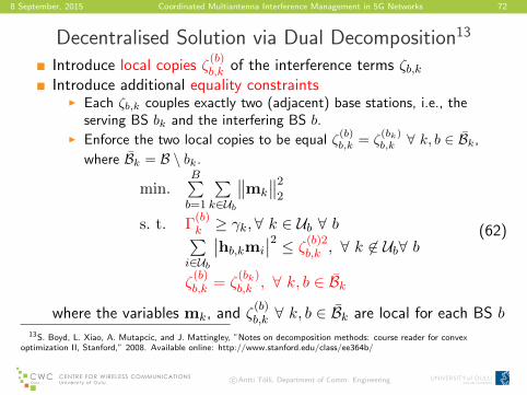
Decentralised Solution via Dual Decomposition13
Introduce local copies ζ(b)b,k of the interference terms ζb,k
Introduce additional equality constraintsI Each ζb,k couples exactly two (adjacent) base stations, i.e., the
serving BS bk and the interfering BS b.I Enforce the two local copies to be equal ζ
(b)b,k = ζ
(bk)b,k ∀ k, b ∈ Bk,
where Bk = B \ bk.
min.B∑b=1
∑k∈Ub
∥∥mk
∥∥22
s. t. Γ(b)k ≥ γk,∀ k ∈ Ub ∀ b∑
i∈Ub
∣∣hb,kmi
∣∣2 ≤ ζ(b)2b,k , ∀ k 6∈ Ub∀ b
ζ(b)b,k = ζ
(bk)b,k , ∀ k, b ∈ Bk
(62)
where the variables mk, and ζ(b)b,k ∀ k, b ∈ Bk are local for each BS b
13S. Boyd, L. Xiao, A. Mutapcic, and J. Mattingley, ”Notes on decomposition methods: course reader for convexoptimization II, Stanford,” 2008. Available online: http://www.stanford.edu/class/ee364b/
c©Antti Tolli, Department of Comm. Engineering
8 September, 2015 Coordinated Multiantenna Interference Management in 5G Networks 73
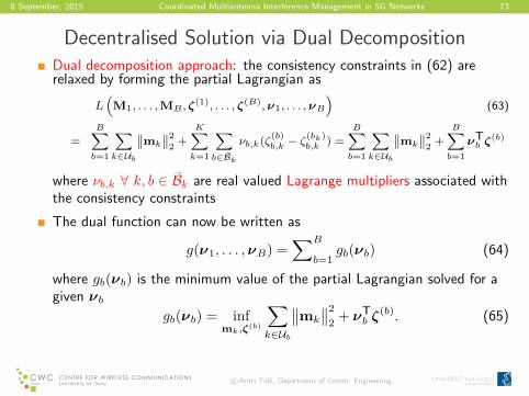
Decentralised Solution via Dual DecompositionDual decomposition approach: the consistency constraints in (62) arerelaxed by forming the partial Lagrangian as
L(M1, . . . ,MB , ζ
(1), . . . , ζ(B),ν1, . . . ,νB
)(63)
=B∑b=1
∑k∈Ub
∥∥mk
∥∥2
2+
K∑k=1
∑b∈Bk
νb,k(ζ(b)b,k − ζ
(bk)b,k ) =
B∑b=1
∑k∈Ub
∥∥mk
∥∥2
2+
B∑b=1
νTb ζ(b)
where νb,k ∀ k, b ∈ Bk are real valued Lagrange multipliers associated withthe consistency constraints
The dual function can now be written as
g(ν1, . . . ,νB) =∑B
b=1gb(νb) (64)
where gb(νb) is the minimum value of the partial Lagrangian solved for agiven νb
gb(νb) = infmk,ζ(b)
∑
k∈Ub
∥∥mk
∥∥22
+ νTb ζ
(b). (65)
c©Antti Tolli, Department of Comm. Engineering

8 September, 2015 Coordinated Multiantenna Interference Management in 5G Networks 74
Decentralised Solution via Dual Decomposition
Finally, the local problem of BS b can be formulated as
min.∑
k∈Ub
∥∥mk
∥∥22
+ νTb ζ
(b)
s. t. Γ(b)k ≥ γk,∀ k ∈ Ub∑
i∈Ub
∣∣hb,kmi
∣∣2 ≤ ζ(b)2b,k , ∀ k 6∈ Ub(66)
where the variables are mk ∀ k ∈ Ub, and ζ(b)
I Locally solved as SOCPs in each BS b with knowledge of νb
The master problem: max. g(ν1, . . . ,νB) with variables νb ∀ bI Solved iteratively with the following updates:
νb,k(t+ 1) = νb,k(t) + µ(ζ(b)b,k(t)− ζ(bk)b,k (t)
),∀ b, k (67)
I t is the iteration/time index, µ is a positive step-size
Feasible solution by using ζb,k(t) = 12(ζ
(bk)b,k (t) + ζ
(b)b,k(t)) in (61)
c©Antti Tolli, Department of Comm. Engineering

8 September, 2015 Coordinated Multiantenna Interference Management in 5G Networks 75
Distributed Algorithm
xx
xx
xx
xx
xx
xx
xx
xx
xx
xx
xx
xx
xx
xx
1=b
3=k
24,1
ceinterferen !"
23,1
ceinterferen !"
21,2
ceinterferen !"
22,2
ceinterferen !"
4=k
2=k
1=k 2=b
!"#$%&'()*+),-.
/0(#1+1#)1&2(3.#(44)
1&2(3+(3(&#()
1&+*35%21*&)
( )21,2
!( )22,2
!( )13,1
! ( )14,1
! ( )11,2
! ( )12,2
! ( )24,1
! ( )23,1
!
Information exchange between adjacent BSs
Real-valued inter-cell interference terms
c©Antti Tolli, Department of Comm. Engineering

8 September, 2015 Coordinated Multiantenna Interference Management in 5G Networks 76
Distributed Algorithm
Always feasible solution: use the average vector ζ(t) in (66)
Feasible γk, ∀ k can be guaranteed even if the update rate of ζ(b)(t)between BSs is slower than the channel coherence time
Special cases with reduced backhaul information exchange
1. Group-specific inter-cell interference constraint,ζb,k = ζb,i ∀ k, i ∈ C, k, i 6∈ Ub
2. BS-specific inter-cell interference constraint, ζb,k = ζb ∀ k 6∈ Ub.3. One common constraint for all BSs (within a given joint processing
area), ζb,k = ζ ∀ k, b.Cases that do not require exchange of ζb,k
1. The constraints ζb,k can be fixed to some values that may depend forexample on the BS- and user-specific operating environment.
2. Zero-forcing for the inter-cell interference, ζb,k = 0 ∀ k, b.
c©Antti Tolli, Department of Comm. Engineering
8 September, 2015 Coordinated Multiantenna Interference Management in 5G Networks 77
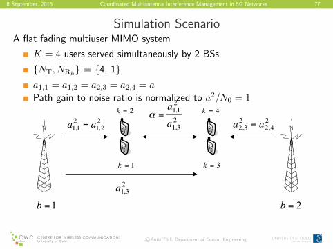
Simulation ScenarioA flat fading multiuser MIMO system
K = 4 users served simultaneously by 2 BSs
{NT, NRk} = {4, 1}a1,1 = a1,2 = a2,3 = a2,4 = a
Path gain to noise ratio is normalized to a2/N0 = 1
1=k
1=b 2=b
22,1
21,1 aa = 2
4,223,2 aa =
3=k
23,1a
23,1
21,1
a
a=α2=k 4=k
c©Antti Tolli, Department of Comm. Engineering
8 September, 2015 Coordinated Multiantenna Interference Management in 5G Networks 78
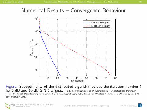
Numerical Results – Convergence Behaviour
10 20 30 40 50 60 70 80
10−6
10−4
10−2
100
102
Iterations [t]
Pdecom
p(t
) −
Popt
0 dB SINR target
10 dB SINR target
Figure: Suboptimality of the distributed algorithm versus the iteration number tfor 0 dB and 10 dB SINR targets. [Tolli, H. Pennanen, and P. Komulainen, ”Decentralized MinimumPower Multi-cell Beamforming with Limited Backhaul Signalling”, IEEE Trans. on Wireless Comm., vol. 10, no. 2, pp. 570 -580, February 2011]
c©Antti Tolli, Department of Comm. Engineering

8 September, 2015 Coordinated Multiantenna Interference Management in 5G Networks 79
Numerical Results – Block Fading
0 3 6 10 20 50−2
0
2
4
6
8
10
12
14
16
Distance α between different user sets [dB]
Tra
nsm
it p
ow
er
[dB
]
ZF for all interference
ZF for inter−cell interference
coordinated, one constr.
coordinated, per BS constr.
coordinated, per user constr.
coherent
Figure: Sum power of {K,B,NT} = {4, 2, 4} system with 0 dB SINR target.[Tolli, H. Pennanen, and P. Komulainen, ”Decentralized Minimum Power Multi-cell Beamforming with Limited BackhaulSignalling”, IEEE Trans. on Wireless Comm., vol. 10, no. 2, pp. 570 - 580, February 2011]
c©Antti Tolli, Department of Comm. Engineering

8 September, 2015 Coordinated Multiantenna Interference Management in 5G Networks 80
Numerical Results – Block Fading
0 3 6 10 20 5018
20
22
24
26
28
30
32
34
36
Distance α between different user sets [dB]
Tra
nsm
it p
ow
er
[dB
]
ZF for all interference
ZF for inter−cell interference
coordinated, one constr.
coordinated, per BS constr.
coordinated, per user constr.
coherent
Figure: Sum power of {K,B,NT} = {4, 2, 4} system with 20 dB SINR target.[Tolli, H. Pennanen, and P. Komulainen, ”Decentralized Minimum Power Multi-cell Beamforming with Limited BackhaulSignalling”, IEEE Trans. on Wireless Comm., vol. 10, no. 2, pp. 570 - 580, February 2011]
c©Antti Tolli, Department of Comm. Engineering

8 September, 2015 Coordinated Multiantenna Interference Management in 5G Networks 81
Time correlated fading - Example
1.12 1.122 1.124 1.126 1.128 1.13 1.132 1.134
x 104
100
101
102
time
Tra
nsm
it po
wer
coordinated, per user constr.coordinated (ideal), per user constr.ZF for inter−cell interference
Figure: Time evolution of the distributed algorithm with 0 dB SINR target,TSfd = 0.1 (e.g., 30 km/h with 2 ms reporting period). [Tolli, H. Pennanen, and P.Komulainen, ”Decentralized Minimum Power Multi-cell Beamforming with Limited Backhaul Signalling”, IEEE Trans. onWireless Comm., vol. 10, no. 2, pp. 570 - 580, February 2011]
TS is the signalling period and fd is the maximum Doppler shift.
c©Antti Tolli, Department of Comm. Engineering

8 September, 2015 Coordinated Multiantenna Interference Management in 5G Networks 82
ExtensionsCognitive underlay cellular network14 - a sum interference constraintis imposed to every primary user k ∈ UP from the secondary BSs BS
∑i∈US
b
∣∣hb,kmi
∣∣2 ≤ φb,k,∀b ∈ BS,∀k ∈ UP
∑b∈BS
φb,k ≤ Φk, ∀k ∈ UP
(68)
(69)
Worst case beamformer design with ellipsoid CSIT uncertainty15,16
hb,k = hb,k + ub,k ∀ b ∈ B, k ∈ UEb,k = {ub,k : ub,kEb,ku
Hb,k ≤ 1} ∀ b ∈ B, k ∈ U
(70)
(71)
where hb,k and ub,k are the estimated channel at the BS and the CSIerror, respectively, and PSD matrix Eb,k defines the CSI accuracy.
14H. Pennanen, A. Tolli and M. Latva-aho, ”Multi-Cell Beamforming with Decentralized Coordination in Cognitive andCellular Networks”, IEEE Transactions on Signal Processing, vol. 62, no. 2, pp. 295 - 308, January 2014
15C. Shen, T. H. Chang, K. Y. Wang, Z. Qiu, and C. Y. Chi, ”Distributed robust multi-cell coordinated beamforming withimperfect CSI: An ADMM approach,” IEEE Trans. Signal Processing, vol. 60, no. 6, pp. 2988 - 3003, Jun. 2012.
16H. Pennanen, A. Tolli and M. Latva-aho, ”Decentralized Robust Beamforming for Coordinated Multi-Cell MISONetworks”, IEEE Signal Processing letters, vol. 21, no. 3, pp. 334 - 338, March 2014
c©Antti Tolli, Department of Comm. Engineering
8 September, 2015 Coordinated Multiantenna Interference Management in 5G Networks 83
Decentralising the Optimal Multi-cell Beamforming viaLarge System Analysis
H. Asgharimoghaddam, A. Tolli & N. Rajatheva, Decentralizing the Optimal Multi-cellBeamforming via Large System Analysis, in Proc. IEEE ICC 2014, Sydney, Australia,June, 2014
H. Asgharimoghaddam, A. Tolli & N. Rajatheva, ”Decentralized Multi-cell BeamformingVia Large System Analysis in Correlated Channels”, in Proc. EUSIPCO 2014, Lisbon,Portugal, September, 2014
H. Asgharimoghaddam, A. Tolli & N. Rajatheva, ”Decentralizing the Optimal Multi-cellBeamforming in Correlated Channels via Large System Analysis”, submitted to IEEETrans on Signal Prog., July 2015
c©Antti Tolli, Department of Comm. Engineering
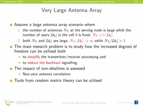
8 September, 2015 Coordinated Multiantenna Interference Management in 5G Networks 84
Very Large Antenna Array
Assume a large antenna array scenario where
1. the number of antennas NT at the serving node is large while thenumber of users |Ub| in the cell b is fixed, NT >> |Ub|
2. both NT and |Ub| are large, NT, |Ub| → ∞ while NT/|Ub| > 1
The main research problem is to study how the increased degrees offreedom can be utilised both
I to simplify the transmitter/receiver processing and
I to reduce the backhaul signalling.
The impact of non-idealities is assessedI Non-zero antenna correlation
Tools from random matrix theory can be utilised
c©Antti Tolli, Department of Comm. Engineering

8 September, 2015 Coordinated Multiantenna Interference Management in 5G Networks 85
System assumptions and research problem
Assumptions:
Local CSI available at eachBS
Linear TX-RX processing
TDD mode – channelreciprocity
NT > Kb
1
2
1 BK-1
K
Problem: Minimum power beamforming
Sum power minimization over BSs with user specificminimum rate/SINR targets
c©Antti Tolli, Department of Comm. Engineering

8 September, 2015 Coordinated Multiantenna Interference Management in 5G Networks 86
Simplified solutionsMatched filter: mk = cbk,kh
Hbk,k
/‖hbk,k‖2, where cbk,k is scaled such
that γk = |hbk,kmk|2/N0
Channel inversion (ZF): the required sum power for a given userallocation Ub is obtained from
∑Bb=1
∑k∈Ub γk‖zb,k‖
22N0 (72)
where the ZF precoders are Zb = [zb,1, . . . , zb,K ] = HHb (HbH
Hb )−1
and where Hb = [hTb,1, . . . ,h
Tb,K ]T, ∀ b.
Fixed ICI thresholds {ζb,k}, with independent optimisation per BS
min.{mk}
∑k∈Ub
∥∥mk
∥∥22
s. t. Γk ≥ γk,∀ k ∈ Ub∑i∈Ub
∣∣hb,kmi
∣∣2 ≤ ζ2b,k, ∀ k 6∈ Ub(73)
c©Antti Tolli, Department of Comm. Engineering
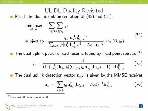
8 September, 2015 Coordinated Multiantenna Interference Management in 5G Networks 87
UL-DL Duality RevisitedRecall the dual uplink presentation of (42) and (61)
minimizeuk,qk
∑
b∈B
∑
k∈Ub
qk
subject toqk|uH
khHbk,k|2
∑l 6=k ql|uH
khHbk,l|2 +N0‖uk‖2
≥γk ∀k∈U(74)
The dual uplink power of each user is found by fixed point iteration17
qk =1
(1 + 1γk
)hbk,k(∑
l∈U qlhHbk,l
hbk,l + I)−1hHbk,k
(75)
The dual uplink detection vector ub,k is given by the MMSE receiver
uk = (∑
l∈Uqlh
Hbk,l
hbk,l +N0I)−1hHbk,k
(76)
17Note that (75) is equivalent to (56)
c©Antti Tolli, Department of Comm. Engineering
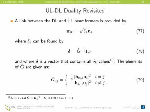
8 September, 2015 Coordinated Multiantenna Interference Management in 5G Networks 88
UL-DL Duality Revisited
A link between the DL and UL beamformers is provided by
mk =√δkuk (77)
where δk can be found by
δ = G−11K (78)
and where δ is a vector that contains all δk values18. The elementsof G are given as:
Gi,j =
{ 1γi|hbi,iui|2 i = j
−|hbj ,iuj |2 i 6= j.(79)
18δk = pk and G = D−1a −G in (49) if ‖uk‖2 = 1
c©Antti Tolli, Department of Comm. Engineering

8 September, 2015 Coordinated Multiantenna Interference Management in 5G Networks 89
Large Dimension Approximation of (75)As N,K →∞ with K/N ∈ (0, B)
qk − qk −→ 0 (80)
almost surely, where the approximated power qk is given as theresult of the convergence of the following iterative formula
q(t+1)k = q
(t)k
γk
e(t)bk,k
. (81)
e(t)bk,k
is the large system approximation of kth user’s SINR atiteration t. The functions ebk,1, ..., ebk,n are given as the uniquenonnegative solution of the following system of equation,
e(t+1)bk,i
=1
NTr{q(t)i θbk,i(
1
N
∑
l∈U
q(t)l θbk,l
1 + e(t)bk,l
+ µbkIN )−1} ∀i. (82)
where θbk,k is the correlation matrix from user k to BS bk,
c©Antti Tolli, Department of Comm. Engineering

8 September, 2015 Coordinated Multiantenna Interference Management in 5G Networks 90
Large Dimension Approximation of (75)
Similarly, the entries of matrix G can be approximated by ,19
Gl,k =
γk(λk)2
l = k
− 1N
e′bk,l
λk(1+e∗bk,l
)2l 6= k
(83)
where, e′bk,l(−1) is the differential of ebk,l(z) with respect to z atpoint z = −1
19H. Asgharimoghaddam, A. Tolli & N. Rajatheva, ”Decentralizing the Optimal Multi-cell Beamforming in CorrelatedChannels via Large System Analysis”, submitted to IEEE Trans on Signal Processing, July 2015
c©Antti Tolli, Department of Comm. Engineering

8 September, 2015 Coordinated Multiantenna Interference Management in 5G Networks 91
Approximation of Intercell Interference TermsFrom (61) and (59), the total ICI from all BSs towards user k is
∑
b 6=bk
ζ2b,k =∑
b6=bk
∑
l∈Ub
|hb,kml|2 (84)
Considering (77), the ICI term ζ2b,k in (84) can be written as follows,
ζ2b,k =∑
l∈Ub
√δl|hb,kul|2 ≈
∑
l∈Ub
√δlGl,k (85)
where δb,l is found from (78) and |hb,kub,l|2 ≈ Gl,k is from (83),
In i.i.d case the ICI can be expressed in a simple form as follows,
ζ2b,i ≈α2b,i
N(1 + e∗b,i)2
∑
j∈Ub
pb,j . (86)
Approximately optimal ICI based on only large scale characteristicsof the user channels.
c©Antti Tolli, Department of Comm. Engineering

8 September, 2015 Coordinated Multiantenna Interference Management in 5G Networks 92
Numerical Examples – Multi-cell case
7 cell wrap-around, K = 28 users dropped randomly
Number of TX antennas per BS, NT = 4− 120
Frequency flat Rayleigh fading
Correlation between adjacent antennas, 0− 0.99
Algorithm 1: Approximation ofuplink/downlink powers anddetection/beamformering vectors.
Algorithm 2: Decentralized beamformingwith approximated ICI values.
c©Antti Tolli, Department of Comm. Engineering

8 September, 2015 Coordinated Multiantenna Interference Management in 5G Networks 93
Numerical Examples
0 10 20 30 40 5072
74
76
78
80
Trial index
Tra
nsm
it S
NR
[dB
]
Transmit SNR Alg 1Transmit SNR Alg 2
0 10 20 30 40 506
8
10
12
Trial index
Res
ulte
d S
INR
[dB
]
Resulted SINR Alg 1Resulted SINR Alg 2
Figure: Transmit powers and SINR variation of Algorithms 1 and 2,N = K = 56, ρ = 0.
c©Antti Tolli, Department of Comm. Engineering

8 September, 2015 Coordinated Multiantenna Interference Management in 5G Networks 94
Numerical Examples
14 28 42 8459
60
61
62
63
64
65
66
67
Number of antennas
Tra
nsm
it S
NR
[dB
]
14 28 42 84−4
−3.5
−3
−2.5
−2
−1.5
MR
T S
INR
(dB
)
MRT SINR
MRTZFCentralizedAlgorithm 2
(a) 0 dB SINR target
14 28 42 8469
70
71
72
73
74
75
76
77
Number of antennas
Tra
nsm
it S
NR
[dB
]
14 28 42 84−0.5
0
0.5
1
1.5
2
2.5
3
3.5
4
MR
T S
INR
(dB
)
MRT SINR
MRTZFCentralizedAlgorithm 2
(b) 10 dB SINR target
Figure: Transmit SNR versus the number of antennas, K = N/2, ρ = 0.8.
c©Antti Tolli, Department of Comm. Engineering

8 September, 2015 Coordinated Multiantenna Interference Management in 5G Networks 95
Numerical Examples
16 28 58 88 12055
60
65
70
75
80
85
90
95
Number of antennas
Tra
nsm
it S
NR
[dB
]
16 28 58 88 120−6.5
−6
−5.5
−5
−4.5
−4
−3.5
−3
−2.5
−2
MR
T S
INR
(dB
)
MRT SINR
MRTZFCentralizedAlgorithm 2
Figure: Transmit SNR vs. the number of antennas, γk = 0 dB, ρ = 0.8,K = 28.
c©Antti Tolli, Department of Comm. Engineering

8 September, 2015 Coordinated Multiantenna Interference Management in 5G Networks 96
OutlineEvolution of multiantenna systemsMIMO with large antenna arraysLinear transceiver design and resource allocation
I Introduction to convex optimisationI Resource allocation and linear transceiver designI Coordinated transceiver optimisationI Coherent vs. coordinated beamforming
Minimum power multicell beamforming with QoS constraintsI Centralised solutionI Decentralised solution via optimisation decompositionI Large system approximation
Throughput optimal linear TX-RX designI Weighted sum rate maximisation (WSRM) via MSE minimisationI WSRM with rate constraintsI Decentralised solution via precoded UL pilotI Bidirectional signalling strategies for dynamic TDDI Mode selection and transceiver design in underlay D2D MIMO
systemsc©Antti Tolli, Department of Comm. Engineering

8 September, 2015 Coordinated Multiantenna Interference Management in 5G Networks 97
Throughput Optimal Linear Transmitter-Receiver Design
S. S. Christensen, R. Agarwal, E. Carvalho, and J. Cioffi, ”Weighted sum-rate maximization using weighted MMSEfor MIMO-BC beamforming design,” IEEE Trans. Wireless Commun., vol. 7, no. 12, pp. 47924799, Dec. 2008.
Q. Shi, M. Razaviyayn, Z.-Q. Luo, and C. He, An iteratively weighted MMSE approach to distributed sum-utilitymaximization for a MIMO interfering broadcast channel, IEEE Trans. Signal Processing, vol. 59, no. 9, pp. 4331 –4340, Sep. 2011
Kaleva, J.; Tolli, A.; Juntti, M.; , ”Weighted Sum Rate Maximization for Interfering Broadcast Channel viaSuccessive Convex Approximation”, Global Communications Conference, 2012. GLOBECOM 2012. IEEE , Dec. 2012
P. Komulainen, A. Tolli & M. Juntti, Effective CSI Signaling and Decentralized Beam Coordination in TDDMulti-Cell MIMO Systems, IEEE Transactions on Signal Processing, vol. 61, no. 9, pp. 2204 – 2218, May 2013
J. Kaleva, A. Tolli & M. Juntti, ”Primal Decomposition based Decentralized Weighted Sum Rate Maximization withQoS Constraints for Interfering Broadcast Channel”, in Proc. IEEE SPAWC 2013, Darmstadt, Germany, June, 2013
J. Kaleva, A. Tolli & M. Juntti, ”Decentralized Beamforming for Weighted Sum Rate Maximization with RateConstraints”, in Proc. IEEE PIMRC 2013 - Workshop on Cooperative and Heterogeneous Cellular Networks, London,UK, Sep. 2013
J. Kaleva, A. Tolli & M. Juntti, ”Decentralized Sum Rate Maximization with QoS Constraints for InterferingBroadcast Channel via Successive Convex Approximation”, IEEE Transactions on Signal Processing, submitted Feb2014, major revision May 2015
c©Antti Tolli, Department of Comm. Engineering

8 September, 2015 Coordinated Multiantenna Interference Management in 5G Networks 98
System Assumptions and Research ProblemAssumptions:
Cellular multi-userMIMO system.
Each user is associatedto single BS(non-cooperative)
TDD and perfect CSIquantization.
User 3User 1
User 2 User 4
BS2BS1
Decentralised beamformer design
Objective: WSRM problem (with user specific rate constraints)I NP-hard problemI Efficient relaxation methods are required for tractability
Focus: low computational complexity and CSI acquisition(pilot/backhaul signalling)
c©Antti Tolli, Department of Comm. Engineering

8 September, 2015 Coordinated Multiantenna Interference Management in 5G Networks 99
WSRM Problem Formulation
Maximise the WSRM over a set of transmit covariance matricesKxk = MkM
Hk
max .Kxk
B∑
b=1
∑
k∈Ub
µk log det(I + R−1k Hbk,kKxkH
Hbk,k
)
s. t.∑
k∈Ub
Tr(Kxk) ≤ Pb, b = 1, . . . , B,(87)
where the interference+noise covariance matrix for user k is
Rk =
K∑
i=1,i 6=kHbi,kKxiH
Hbi,k
+N0I (88)
Difficult non-convex optimisation problem in general (except whenB = 1 or Bk = B ∀ k)
c©Antti Tolli, Department of Comm. Engineering

8 September, 2015 Coordinated Multiantenna Interference Management in 5G Networks 100
MSE Reformulation
The MSE of the received data vector dk = UHk yk for user k is
Ek , E[(dk − dk)(dk − dk)H]
= I−UHkHbk,kMk − (UH
kHbk,kMk)H + UH
kRkUk,(89)
where the received signal covariance Rk for user k is
Rk , E[ykyHk ] =
K∑
i=1
Hbi,kMiMHi HH
bi,k+ σ2kI. (90)
When the MMSE receiver (37) is employed in (89), the MSE matrixbecomes
EMMSEk = I−MH
kHHbk,k
R−1k Hbk,kMk (91)
Furthermore
EMMSEk =
(I + MH
kHHbk,k
R−1b,kHbk,kMk
)−1(92)
c©Antti Tolli, Department of Comm. Engineering

8 September, 2015 Coordinated Multiantenna Interference Management in 5G Networks 101
MSE Reformulation
Applying (92) to (87), we can reformulate the WSRMax objective asminMk
∑Kk=1 µk log det
(EMMSEk
)– still non-convex
Local solution: introduce new variables and split the problem intosolvable subproblems
min .Uk,Mk,Ek
K∑
k=1
µk log det(Ek
)
s. t. Ek 4 Ek, k = 1, . . . ,K,Mk ∈ Pbk , k = 1, . . . ,K,
(93)
where Pb, b = 1, . . . , B are separable convex per-BS powerconstraints, and the relaxation Ek 4 Ek, k = 1, . . . ,K bounds theachieved MSE20.
20The relaxation tightness follows from the matrix monotonicity of the determinant function [Boyd&Vandenbergh].
c©Antti Tolli, Department of Comm. Engineering

8 September, 2015 Coordinated Multiantenna Interference Management in 5G Networks 102
MSE ReformulationFor fixed Mk, the rate maximizing Uk are solved from the roots ofthe Lagrangian of (93) as Uk = R−1k Hbk,kMk, k = 1, . . . ,KFor fixed receive beamformers Uk, the concave objective function isiteratively linearised w.r.t Ek.21
The linearised convex subproblem in ith iteration is given as
min .Mk,E
ik
K∑
k=1
µkTr(Wi
kEik
)
s. t. Ek 4 Eik, k = 1, . . . ,K,
Mk ∈ Pbk , k = 1, . . . ,K,
(94)
where Wik = Gi
k and Gik = ∇Ei−1
k
(log det
(Ei−1k
))= [Ei−1
k ]−1 for
all k = 1, . . . ,K.Monotonic improvement of the objective of (93) on every iteration.
21This method in the context of weighted sum rate maximisation was established in [Shi et al, TSP’11], where it wasreferred to as (iteratively) weighted MMSE minimization.
c©Antti Tolli, Department of Comm. Engineering

8 September, 2015 Coordinated Multiantenna Interference Management in 5G Networks 103
TX precoder adaptation stepThe relaxation Ek 4 Ei
k is tight → Replace Eik with Ek (89) in the
objective of (94)Local convex problem for each BS b
min∑
k∈Ub
(−2µkTr(WkU
HkHbk,kMk)
+
K∑
i=1
µiTr(MHkHH
bk,iUiWiU
Hi Hbk,iMk)
)
s. t.∑
k∈Ub
Tr(MkMHk ) ≤ Pb
(95)
Iterative solution from the KKT conditions
Mk =
(K∑
i=1
HHbk,i
UiWiUHi Hbk,i + νbkI
)−1HHbk,k
UkWk (96)
where the optimal νbk22 is found via bisection
22dual variable related to the power constraintc©Antti Tolli, Department of Comm. Engineering
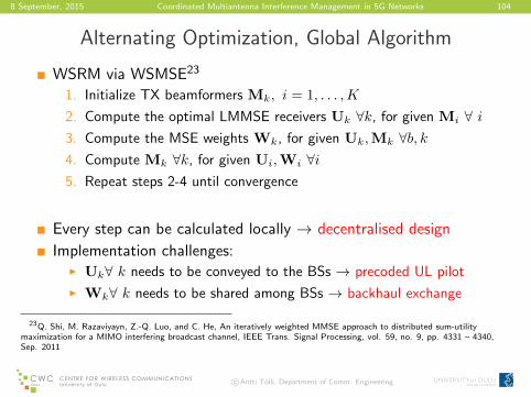
8 September, 2015 Coordinated Multiantenna Interference Management in 5G Networks 104
Alternating Optimization, Global Algorithm
WSRM via WSMSE23
1. Initialize TX beamformers Mk, i = 1, . . . ,K
2. Compute the optimal LMMSE receivers Uk ∀k, for given Mi ∀ i3. Compute the MSE weights Wk, for given Uk,Mk ∀b, k4. Compute Mk ∀k, for given Ui,Wi ∀i5. Repeat steps 2-4 until convergence
Every step can be calculated locally → decentralised design
Implementation challenges:I Uk∀ k needs to be conveyed to the BSs → precoded UL pilot
I Wk∀ k needs to be shared among BSs → backhaul exchange
23Q. Shi, M. Razaviyayn, Z.-Q. Luo, and C. He, An iteratively weighted MMSE approach to distributed sum-utilitymaximization for a MIMO interfering broadcast channel, IEEE Trans. Signal Processing, vol. 59, no. 9, pp. 4331 – 4340,Sep. 2011
c©Antti Tolli, Department of Comm. Engineering

8 September, 2015 Coordinated Multiantenna Interference Management in 5G Networks 105
Alternative WSRM Problem Formulation
Data stream specific processing
max .mk,l,uk,l
B∑
b=1
∑
k∈Ub
µk
(mk∑
l=1
log2 (1 + Γk,l)
)
s. t.∑
k∈Ub
mk∑
l=1
‖mk,l‖2 ≤ Pb, b = 1, . . . , B,
(97)
where SINR of data stream l of user k is
Γk,l =|uHk,lHbk,kmk,l|2
K∑
i=1
mi∑
j=1(i,j)6=(k,l)
|uHk,lHbi,kmi,j |2 + σ2k‖uk,l‖2
.
c©Antti Tolli, Department of Comm. Engineering

8 September, 2015 Coordinated Multiantenna Interference Management in 5G Networks 106
Preliminaries
Rate maximising receive beamformers for fixed precoders are
uk,l =
K∑
j=1
mk∑
l=1
Hbj ,kmj,lmHj,lH
Hbj ,k
+ Iσ2k
−1
Hbk,lmk,l ∀ (k, l).
Mean-squared error (MSE) for data stream l of user k is defined as
εk,l , |1− uHk,lHbk,kmk,l|2+
K∑
i=1
mi∑
j=1(i,j)6=(k,l)
|uHk,lHbi,kmj,i|2 + σ2k‖uk,l‖2.
MSE and SINR have following relation (assuming MMSE receivebeamformers)
ε−1k,l = Γk,l + 1.
c©Antti Tolli, Department of Comm. Engineering

8 September, 2015 Coordinated Multiantenna Interference Management in 5G Networks 107
MSE formulation
max .tk,l,mk,l
B∑
b=1
∑
k∈Ub
µk
(mk∑
l=1
log2 (g(tk,l))
)
s. t. εk,l ≤ [g(tk,l)]−1 ∀ (k, l),
∑
k∈Ub
mk∑
l=1
‖mk,l‖2 ≤ Pb, b = 1, . . . , B.
(98)
MSE constraint can be formulated as a difference of convexfunctions program (DCP), by introducing upper boundary g(tk,l) foreach MSE term εk,l
εk,l ≤ [g(tk,l)]−1 ⇔ εk,l − [g(tk,l)]
−1 ≤ 0.
Note that the problem is still non-convex.I g(tk,l) is monotonic and log-concave.I [g(tk,l)]
−1 is convex.
c©Antti Tolli, Department of Comm. Engineering

8 September, 2015 Coordinated Multiantenna Interference Management in 5G Networks 108
Successive convex approximation
At each point t(i)k,l ∀ (k, l), (98) is approximated as convex problem
by taking first-order Taylor series approximation of the MSE upperboundary.
f(x, x0) , f(x0) + (x− x0) ∂∂xf(x0). (99)
Convex, ith, approximation of (98) at point t(i)k,l ∀ (k, l) is
max .tk,l,mk,l
B∑
b=1
∑
k∈Ub
µk
(mk∑
l=1
log2 (g(tk,l))
)
s. t. εk,l ≤ g(tk,l, t(i)k,l) ∀ (k, l)
∑
k∈Ub
mk∑
l=1
‖mk,l‖2 ≤ Pb, b = 1, . . . , B.
(100)
c©Antti Tolli, Department of Comm. Engineering

8 September, 2015 Coordinated Multiantenna Interference Management in 5G Networks 109
SCA algorithm outline
1: Initialize t(1)k,l ∀ (k, l) in such a away that
[g(t
(1)k,l )]−1
= 1.
2: Initialize precoders mk,l ∀ (k, l) in such a way that sum powerconstraints are satisfied.
3: Set i = 1.4: repeat5: Generate MMSE receive beamformers uk,l ∀ (k, l).6: repeat7: Solve precoders mk,l ∀ (k, l) and tk,l ∀ (k, l) from (100).8: i = i+ 1.9: t
(i)k,l = tk,l ∀ (k, l).
10: until Desired level of convergence has been reached.11: until Desired level of convergence has been reached.
c©Antti Tolli, Department of Comm. Engineering

8 September, 2015 Coordinated Multiantenna Interference Management in 5G Networks 110
Exponential MSE boundary functions
An import class of functions for MSE boundary are exponentialfunctions g(tk,l) = αtk,l , where α > 0.
Allow efficient iterative solution and distributed design.
max .tk,l,mk,l
B∑
b=1
∑
k∈Ub
µk
(mk∑
l=1
log2(α)tk,l
)
s. t. εk,l ≤ α−t(i)k,l − log(α)(tk,l − t(i)k,l)α
−t(i)k,l ∀ (k, l)∑
k∈Ub
mk∑
l=1
‖mk,l‖2 ≤ Pb, b = 1, . . . , B.
(101)
c©Antti Tolli, Department of Comm. Engineering

8 September, 2015 Coordinated Multiantenna Interference Management in 5G Networks 111
Solution via KKT Conditions
Beamformers mk,l can be solved from the roots of the gradient ofthe Lagrangian as
mk,l =
∑
(i,j)
λi,jHHbk,i
ui,juHi,jHbk,i + νbkI
−1
λk,lHHbk,k
uk,l. (102)
The Lagrange multipliers are λk,l = µkαt(i)k,l
log(α) and optimal νb ∀ b arefound by bisection.
t(i+1)k,l can be found from the corresponding complementary
slackness constraint to be
t(i+1)k,l = t
(i)k,l +
1
log(α)(1− εk,lαt
(i)k,l) ∀ (k, l).
Here, term 1log(α) can be seen as step size for an exact line search.
c©Antti Tolli, Department of Comm. Engineering
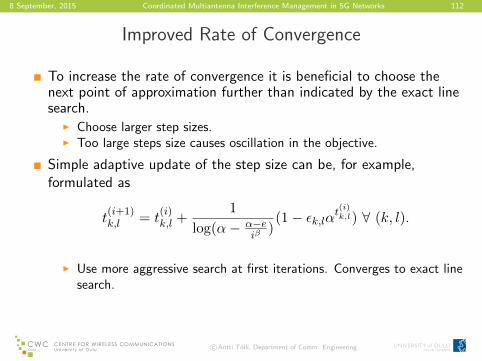
8 September, 2015 Coordinated Multiantenna Interference Management in 5G Networks 112
Improved Rate of Convergence
To increase the rate of convergence it is beneficial to choose thenext point of approximation further than indicated by the exact linesearch.
I Choose larger step sizes.I Too large steps size causes oscillation in the objective.
Simple adaptive update of the step size can be, for example,formulated as
t(i+1)k,l = t
(i)k,l +
1
log(α− α−eiβ
)(1− εk,lαt
(i)k,l) ∀ (k, l).
I Use more aggressive search at first iterations. Converges to exact linesearch.
c©Antti Tolli, Department of Comm. Engineering

8 September, 2015 Coordinated Multiantenna Interference Management in 5G Networks 113
Numerical Results
5 10 15 20 25 30 354
6
8
10
12
14
16
18
20
22
SNR (dB)
Su
m r
ate
(b
its/H
z/s
)
SCA (Imax
= 3)
[4] (Imax
= 3)
[3] (Imax
= 3)
SCA (Imax
= 6)
[4] (Imax
= 6)
[3] (Imax
= 6)
SCA (Imax
= 10)
[4] (Imax
= 10)
[3] (Imax
= 10)
10 Iterations
6 Iterations
3 Iterations
Figure: Impact of the limited number of iterations to the achievable sum ratewith NT = 4, NR = 2, K = 8. [Kaleva, J.; Tolli, A.; Juntti, M.; , ”Weighted Sum Rate Maximization forInterfering Broadcast Channel via Successive Convex Approximation”, Global Communications Conference, 2012.GLOBECOM 2012. IEEE , Dec. 2012]
[3] Q. Shi, M. Razaviyayn, Z.-Q. Luo, and C. He, An iteratively weighted MMSE approach to distributed sum-utility maximization for a MIMO
interfering broadcast channel, IEEE Trans. Signal Processing, Sep. 2011.
[4] T. Bogale and L. Vandendorpe, Weighted sum rate optimization for downlink multiuser MIMO coordinated base station systems: Centralized and
distributed algorithms, IEEE Trans. Signal Processing, Dec. 2011.
c©Antti Tolli, Department of Comm. Engineering

8 September, 2015 Coordinated Multiantenna Interference Management in 5G Networks 114
WSRmax with QoS Constraints24
Objective: WSRmax with per user QoS constraints
max .mk,l,uk,l
B∑
b=1
∑
k∈Ub
µk
(mk∑
l=1
log2 (1 + Γk,l)
)
s. t.
mk∑
l=1
log2 (1 + Γk,l) ≥ Rk ∀ k = 1, . . . ,K,
∑k∈Ub
∑mkl=1 ‖mk,l‖2 ≤ Pb, b = 1, . . . , B,
where SINR of data stream l of user k is
Γk,l =|uHk,lHbk,kmk,l|2
∑Ki=1
∑mij=1,
(i,j)6=(k,l)
|uHk,lHbi,kmi,j |2 + σ2k‖uk,l‖2
.
24J. Kaleva, A. Tolli & M. Juntti, ”Decentralized Beamforming for Weighted Sum Rate Maximization with RateConstraints”, in Proc. IEEE PIMRC 2013 - Workshop on Cooperative and Heterogeneous Cellular Networks, London, UK,Sep. 2013
c©Antti Tolli, Department of Comm. Engineering

8 September, 2015 Coordinated Multiantenna Interference Management in 5G Networks 115
MSE Reformulation
Introduce upper boundary 2tk,l for each MSE term εk,l
maxtk,l,mk,l
B∑
b=1
∑
k∈Ub
µk
(mk∑
l=1
tk,l
)
s. t. εk,l ≤ 2−tk,l ∀ (k, l),mk∑
l=1
tk,l ≥ Rk, k = 1, . . . ,K,
∑
k∈Ub
mk∑
l=1
‖mk,l‖2 ≤ Pb, b = 1, . . . , B,
Difference of convex functions program (DCP), εk,l − 2tk,l ≤ 0
Successive convex (linear) approximation is used to approximate theMSE bounds 2tk,l ∀ (k, l) iteratively.
c©Antti Tolli, Department of Comm. Engineering
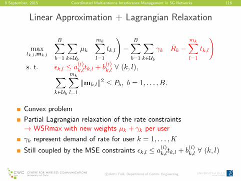
8 September, 2015 Coordinated Multiantenna Interference Management in 5G Networks 116
Linear Approximation + Lagrangian Relaxation
maxtk,l,mk,l
B∑
b=1
∑
k∈Ub
µk
(mk∑
l=1
tk,l
)−
B∑
b=1
∑
k∈Ub
γk
(Rk −
mk∑
l=1
tk,l
)
s. t. εk,l ≤ a(i)k,ltk,l + b(i)k,l ∀ (k, l),
∑
k∈Ub
mk∑
l=1
‖mk,l‖2 ≤ Pb, b = 1, . . . , B.
Convex problem
Partial Lagrangian relaxation of the rate constraints→ WSRmax with new weights µk + γk per user
γk represent demand of rate for user k = 1, . . . ,K
Still coupled by the MSE constraints εk,l ≤ a(i)k,ltk,l + b(i)k,l ∀ (k, l)
c©Antti Tolli, Department of Comm. Engineering

8 September, 2015 Coordinated Multiantenna Interference Management in 5G Networks 117
Iterative SolutionTransmit beamformers are obtained directly from the KKT conditions as
mk,l = K†k,lHHbk,l
uk,lλk,l ∀ (k, l),
where
Kk,l =K∑
i=1
mi∑
j=1
λi,jHHbk,i
ui,juHi,jHbk,i + Iνb.
MSE constraint related dual variables (MSE weights) can be written inclosed form as
λk,l = (µk + γk)/a(i)k,l ∀ (k, l).
I Depends only on the point of approximation and rate demand dual variablesγk = 1, . . . ,K.
The rate demand weight factors γk ∀ k = 1, . . . ,K are updated according tothe subgradients of the corresponding rate constraints
γ(i+1)k =
(γ(i)k + β
(i)k
(Rk +
mk∑
l=1
t(i)k,l)
))+
.
All steps can be executed locally at each BS / terminal
c©Antti Tolli, Department of Comm. Engineering

8 September, 2015 Coordinated Multiantenna Interference Management in 5G Networks 118
Features & Issues
Computational complexity
Receive beamformers uk,l can be solved in a closed form (LMMSE)
Transmit beamformers mk,l require simple bisection over νb
Dual variables λk,l are solved in a closed form
Feasibility
Each step is not required to be feasible (rate constraints)
Possibly strictly feasible only after convergence
Initialization
Does not require feasible initial pointI Simplifies distributed design
c©Antti Tolli, Department of Comm. Engineering

8 September, 2015 Coordinated Multiantenna Interference Management in 5G Networks 119
Algorithm Outline
1: Initialize precoders mk,l ∀ (k, l).2: Initialize γk,l = 0 ∀ (k, l).3: repeat4: Generate LMMSE receive beamformers uk,l ∀ (k, l).5: repeat6: Measure MSE εk,l ∀ (k, l).7: Update rate demand variables γk ∀ k = 1, . . . ,K.8: Assign weights λk,l ∀ (k, l).9: Exchange weights λk,l ∀ (k, l) between the adjacent BSs.
10: Solve transmit beamformers mk,l ∀ (k, l).11: until Desired level of convergence has been reached or i > Imax.12: until Desired level of convergence has been reached or j > Jmax.
c©Antti Tolli, Department of Comm. Engineering
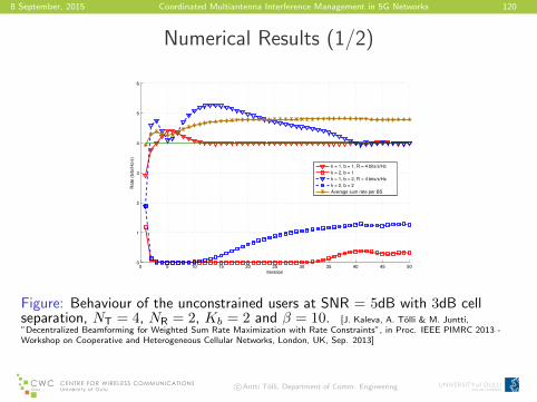
8 September, 2015 Coordinated Multiantenna Interference Management in 5G Networks 120
Numerical Results (1/2)
0 5 10 15 20 25 30 35 40 45 500
1
2
3
4
5
6
Iteration
Rate
(b
its/H
z/s
)
k = 1, b = 1, R = 4 bits/s/Hz
k = 2, b = 1
k = 1, b = 2, R = 4 bits/s/Hz
k = 2, b = 2
Average sum rate per BS
Figure: Behaviour of the unconstrained users at SNR = 5dB with 3dB cellseparation, NT = 4, NR = 2, Kb = 2 and β = 10. [J. Kaleva, A. Tolli & M. Juntti,”Decentralized Beamforming for Weighted Sum Rate Maximization with Rate Constraints”, in Proc. IEEE PIMRC 2013 -Workshop on Cooperative and Heterogeneous Cellular Networks, London, UK, Sep. 2013]
c©Antti Tolli, Department of Comm. Engineering

8 September, 2015 Coordinated Multiantenna Interference Management in 5G Networks 121
Numerical Results (2/2)
0 5 10 15 20 25 30 35 40 45 500
1
2
3
4
5
6
Iteration
Rate
(b
its/H
z/s
)
k = 1, b = 1, R = 4 bits/s/Hz
k = 2, b = 1, R = 2 bits/s/Hz
k = 3, b = 1, R = 2 bits/s/Hz
k = 1, b = 2, R = 4 bits/s/Hz
k = 2, b = 2, R = 2 bits/s/Hz
k = 3, b = 2, R = 2 bits/s/Hz
Figure: Convergence at SNR = 15dB with 3dB cell separation, NT = 4,NR = 2, Kb = 3 and β = 4. [J. Kaleva, A. Tolli & M. Juntti, ”Decentralized Beamforming for WeightedSum Rate Maximization with Rate Constraints”, in Proc. IEEE PIMRC 2013 - Workshop on Cooperative and HeterogeneousCellular Networks, London, UK, Sep. 2013]
c©Antti Tolli, Department of Comm. Engineering

8 September, 2015 Coordinated Multiantenna Interference Management in 5G Networks 122
Numerical Results - ADMM extension
0 10 20 30 40 50 601
1.5
2
2.5
3
3.5
4
4.5
5
Iteration
Rat
e (b
its/H
z/s)
Alternating Direction Method of Multipliers (ADMM).
0 10 20 30 40 50 600
0.5
1
1.5
2
2.5
3
3.5
4
4.5
Iteration
Rat
e (b
its/H
z/s)
Dual Decomposition.
k = 1k = 2k = 3k = 4
Figure: Convergence of the ADMM and dual decomposition methods withB = 2,Kb = 2, NT = 2, NR = 2, Rk = 3bits/Hz/sec, β = 2, ρ = 1.5, χ = 3dBand SNR = 15dB. [J. Kaleva, A. Tolli and M. Juntti, ”Rate Constrained Decentralized Beamforming for MIMOInterfering Broadcast Channel”, PIMRC’15, Hong Kong, June, 2015]
c©Antti Tolli, Department of Comm. Engineering
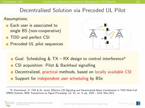
8 September, 2015 Coordinated Multiantenna Interference Management in 5G Networks 123
Decentralised Solution via Precoded UL Pilot
Assumptions:
Each user is associated tosingle BS (non-cooperative)
TDD and perfect CSI
Precoded UL pilot sequences
1
2
1 BK-1
K
Goal: Scheduling & TX – RX design to control interferencea
CSI acquisition: Pilot & Backhaul signalling
Decentralized, practical methods, based on locally available CSI
Support for independent user scheduling by BSs
aP. Komulainen, A. Tolli & M. Juntti, Effective CSI Signaling and Decentralized Beam Coordination in TDD Multi-CellMIMO Systems, IEEE Transactions on Signal Processing, vol. 61, no. 9, pp. 2204 – 2218, May 2013
c©Antti Tolli, Department of Comm. Engineering

8 September, 2015 Coordinated Multiantenna Interference Management in 5G Networks 124
Strategy A: Global AlgorithmEach BS b calculates own weights Wk ∀ k ∈ Ub : distribute viabackhaulEach BS calculates own precoders Mk ∀ k ∈ Ub : use for datatransmission
Each UE calculates own receiver Uk : use for reception and ULsounding
Slow convergence
c©Antti Tolli, Department of Comm. Engineering

8 September, 2015 Coordinated Multiantenna Interference Management in 5G Networks 125
Strategy B: Separate Channel Sounding (CS) and BusyBurst (BB) Pilots
CS pilot Qk whitens the inter-cell interference at terminal k so thatQHkQk = R−1k , where Rk =
∑i 6∈Ubk
Hbi,kMiMHi HH
bi,k+N0I
The MSE weights calculated by the terminals can be incorporated to
the uplink BB signaling so that pilot precoder is W12k Uk
Allows local iterationsno backhaul required
c©Antti Tolli, Department of Comm. Engineering

8 September, 2015 Coordinated Multiantenna Interference Management in 5G Networks 126
Strategy C: Cell-specific Iterations with CS Only
Allows local iterationsfast convergence
c©Antti Tolli, Department of Comm. Engineering

8 September, 2015 Coordinated Multiantenna Interference Management in 5G Networks 127
Numerical Results: Setup
Two 4-antenna BSs, five 2-antenna UEs per BS
Cell separation defined as a1/a2
Uncorrelated Rayleigh (quasistatic) fading
c©Antti Tolli, Department of Comm. Engineering

8 September, 2015 Coordinated Multiantenna Interference Management in 5G Networks 128
Numerical Results: Convergence
2 4 6 8 10 12 14 16 18 204
6
8
10
12
14
16
18
Frame
Su
m r
ate
per
BS
[b
its/
Hz/
s]
M = 4, N = 2, K = 5, SNR = 25dB, cell sep. = 0dB
Alg. 1 (matrix weighted)
Strat. A: BB only
Strat. B: BB+CS
Strat. C: CS only
Strat. A (AP constraints)
Non−cooperative
Figure: Average convergence of the sum rate at 0dB cell separation, at 25dBSNR. [P. Komulainen, A. Tolli & M. Juntti, Effective CSI Signaling and Decentralized Beam Coordination in TDDMulti-Cell MIMO Systems, IEEE Transactions on Signal Processing, vol. 61, no. 9, pp. 2204 – 2218, May 2013]
c©Antti Tolli, Department of Comm. Engineering

8 September, 2015 Coordinated Multiantenna Interference Management in 5G Networks 129
Bidirectional Signalling Strategies for Dynamic TDD
P. Jayasinghe, A. Tolli, J. Kaleva and M. Latva-aho, ”Bi-directionalSignaling for Dynamic TDD with Decentralized Beamforming” ICCWorkshop on Small Cell and 5G Networks (SmallNets), London, UK, June,2015
P. Jayasinghe, A. Tolli, and M. Latva-aho, ”Bi-directional SignalingStrategies for Dynamic TDD Networks” IEEE SPAWC, Stockholm,Sweden, July, 2015
METIS Deliverable D3.3 on ”Final performance results and consolidatedview on the most promising multi-node/multi-antenna transmissiontechnologies” (A. Tolli & P. Jayasinghe), https://www.metis2020.com/
c©Antti Tolli, Department of Comm. Engineering

8 September, 2015 Coordinated Multiantenna Interference Management in 5G Networks 130
Background & Introduction
Figure: Dynamic TDD system
The load variation between adjacent small cells can be significant.
Fixed UL/DL switching would be highly suboptimal.
With the flexible UL/DL allocation provides large potential gains inspectral efficiency → dynamic traffic aware TDD transmission
Allowing such flexibility makes obviously the interferencemanagement considerably more challenging.
c©Antti Tolli, Department of Comm. Engineering

8 September, 2015 Coordinated Multiantenna Interference Management in 5G Networks 131
Interference scenarios
Figure: Interference at DL terminal Figure: Interference at UL BS
Additional interference associated with the dynamic TDDI UL-to-DL interference.I DL-to-UL interference.
Interference mitigated by coordinated beamforming.More measurements and info exchange also at the terminal side
c©Antti Tolli, Department of Comm. Engineering

8 September, 2015 Coordinated Multiantenna Interference Management in 5G Networks 132
Synchronous TDD - System Model
Assumptions:
Multi-cell multiuser MIMO
Each user served by one BS
Linear TX-RX processing
TDD and perfect CSI
Coordination via pilot andbackhaul signaling
1
2
1 BK-1
K
Problem: System utility maximization
low computational complexity and CSI acquisition
Impact of forward-backward training on the system performance
c©Antti Tolli, Department of Comm. Engineering

8 September, 2015 Coordinated Multiantenna Interference Management in 5G Networks 133
Bi-directional training
Figure: Backward-Forward training structure [Changxin Shi; Berry, R.A.; Honig, M.L.,”Bi-Directional Training for Adaptive Beamforming and Power Control in Interference Networks,” Signal Processing, IEEETransactions on , vol.62, no.3, pp.607–618, Feb.1, 2014]
Bidirectional training(BIT) phase is used in the beginning of eachTDD frame to speed up the convergence of the iterative algorithms
A number of blocks of pilots are alternately transmitted in thedownlink and the uplink
c©Antti Tolli, Department of Comm. Engineering
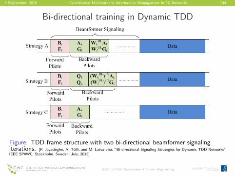
8 September, 2015 Coordinated Multiantenna Interference Management in 5G Networks 134
Bi-directional training in Dynamic TDD
Figure: TDD frame structure with two bi-directional beamformer signalingiterations. [P. Jayasinghe, A. Tolli, and M. Latva-aho, ”Bi-directional Signaling Strategies for Dynamic TDD Networks”IEEE SPAWC, Stockholm, Sweden, July, 2015]
c©Antti Tolli, Department of Comm. Engineering
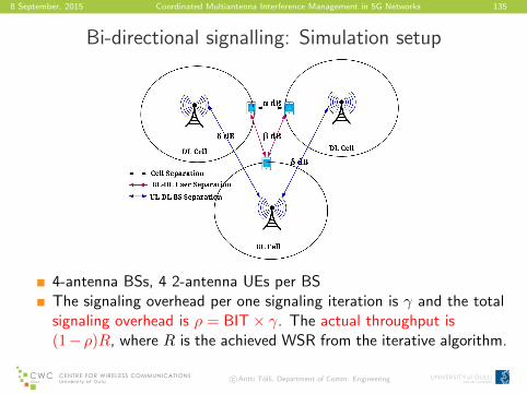
8 September, 2015 Coordinated Multiantenna Interference Management in 5G Networks 135
Bi-directional signalling: Simulation setup
4-antenna BSs, 4 2-antenna UEs per BSThe signaling overhead per one signaling iteration is γ and the totalsignaling overhead is ρ = BIT× γ. The actual throughput is(1− ρ)R, where R is the achieved WSR from the iterative algorithm.
c©Antti Tolli, Department of Comm. Engineering

8 September, 2015 Coordinated Multiantenna Interference Management in 5G Networks 136
Synchronous 2-cell Downlink, Strategy A
0 0.05 0.1 0.15 0.2 0.25 0.3 0.35 0.4 0.45 0.56
8
10
12
14
16
18
20
22
Overhead
ActualSum
Rate
(SNR
=10dB)
α = 0 dB & γ = 0.01
α = 0 dB & γ = 0.02
α = 0 dB , uncoordinated
α = 12 dB & γ = 0.01
α = 12 dB & γ = 0.02
α = 12 dB , uncoordinated
0 0.05 0.1 0.15 0.2 0.25 0.3 0.35 0.4 0.45 0.55
10
15
20
25
30
Overhead
ActualSum
Rate
(SNR
=20dB)
α = 0 dB & γ = 0.01
α = 0 dB & γ = 0.02
α = 0 dB , uncoordinated
α = 12 dB & γ = 0.01
α = 12 dB & γ = 0.02
α = 12 dB , uncoordinated
Peak Rate
Peak Rate
Figure: Actual Sum rate vs overhead with different SNR (10, 20 dB) values. [P.Jayasinghe, A. Tolli, J. Kaleva and M. Latva-aho, ”Bi-directional Signaling for Dynamic TDD with DecentralizedBeamforming” ICC Workshop on Small Cell and 5G Networks (SmallNets), London, UK, June, 2015]
c©Antti Tolli, Department of Comm. Engineering

8 September, 2015 Coordinated Multiantenna Interference Management in 5G Networks 137
Dynamic TDD 3-cell, Strategy A
0 0.05 0.1 0.15 0.2 0.25 0.3 0.35 0.4 0.45 0.510
15
20
25
30
35
Overhead
ActualSum
Rate
α = 0dB ,β = 3dB, δ = 6dB, γ = 0.01
α = 0dB ,β = 3dB, δ = 6dB uncoordinated
α = 0dB ,β = 9dB, δ = 12dB, γ = 0.01
α = 0dB ,β = 9dB, δ = 12dB uncoordinated
α = 6dB ,β = 3dB, δ = 6dB, γ = 0.01
α = 6dB ,β = 3dB, δ = 6dB uncoordinated
α = 6dB ,β = 9dB, δ = 12dB, γ = 0.01
α = 6dB ,β = 9dB, δ = 12dB uncoordinated
Peak Rate
Figure: Actual sum rate vs overhead at SNR = 20 dB, with diferent α, β, δ. [P.Jayasinghe, A. Tolli, J. Kaleva and M. Latva-aho, ”Bi-directional Signaling for Dynamic TDD with DecentralizedBeamforming” ICC Workshop on Small Cell and 5G Networks (SmallNets), London, UK, June, 2015]
c©Antti Tolli, Department of Comm. Engineering

8 September, 2015 Coordinated Multiantenna Interference Management in 5G Networks 138
Time-correlated Fading Scenario
50 55 60 65 70 75 80 85 90 95 10014
16
18
20
22
24
26
Channel Number
AverageActu
alSum
Rate
BIT =1, no reset
BIT =3, reset = 10
BIT =5, reset = 10
BIT =10, reset =10
Figure: Average sum rate over time-correlated channel at SNR = 20 dB withγ = 0.01. [P. Jayasinghe, A. Tolli, J. Kaleva and M. Latva-aho, ”Bi-directional Signaling for Dynamic TDD withDecentralized Beamforming” ICC Workshop on Small Cell and 5G Networks (SmallNets), London, UK, June, 2015]
c©Antti Tolli, Department of Comm. Engineering

8 September, 2015 Coordinated Multiantenna Interference Management in 5G Networks 139
Comparison of different signalling strategies
0 0.05 0.1 0.15 0.2 0.25 0.3 0.35 0.4 0.45 0.510
12
14
16
18
20
22
24
26
28
Overhead
Actu
alRate
atSNR
=20dB
Strategy A
Strategy B
Strategy C
Uncoordinated method
Figure: Actual sum rate at SNR = 20dB vs overhead for different bi-directionalsignaling strategies.
c©Antti Tolli, Department of Comm. Engineering

8 September, 2015 Coordinated Multiantenna Interference Management in 5G Networks 140
Mode Selection and Transceiver Design in Underlay D2DMIMO Systems
A. Tolli, J. Kaleva and P. Komulainen, ”Mode Selection and TransceiverDesign for Rate Maximization in Underlay D2D MIMO Systems”, IEEEICC, London, UK, June, 2015
A. Ghazanfari, A. Tolli and J. Kaleva, ”Joint Power Loading and ModeSelection for Network-assisted Device-to-Device Communication”, IEEEICC, London, UK, June, 2015
c©Antti Tolli, Department of Comm. Engineering

8 September, 2015 Coordinated Multiantenna Interference Management in 5G Networks 141
System assumptions and research problemAssumptions:
One multiantenna BS in charge of LD2D pairs
K = 2L multiantenna users in total
Linear TX-RX processing
Centralized processing
Half-duplex nodes
Slotted transmission - UL(1) andDL(2) slots
Problem: Weighted sum ratemaximization (WSR)
Aggregate sum of end-to-end datarates carried via uplink, downlink,and D2D links
c©Antti Tolli, Department of Comm. Engineering

8 September, 2015 Coordinated Multiantenna Interference Management in 5G Networks 142
Optimization problemThe optimization objective is to maximize the aggregate sum of E2Edata rates carried via uplink(1), downlink(2), and D2D links
max .
L∑
l=1
µl
(R
(1)l +R
(2)l + min(R
(1)l , R
(2)l ))
(103a)
s. t. ‖M(1)l ‖2F + ‖Fl‖2F ≤ Pil∀ l (103b)
‖M(2)l ‖2F ≤ Pil∀ l (103c)
L∑
l=1
‖Bl‖2F ≤ PB. (103d)
Opt. variables: TX precoders for link l
M(1)l ,M
(2)l for direct D2D TX in time slots (1) and (2)
Fl for UL TX in time slot (1)
Bl for DL TX in time slot (2)
c©Antti Tolli, Department of Comm. Engineering

8 September, 2015 Coordinated Multiantenna Interference Management in 5G Networks 143
Reformulation via MSE minimization
By writing the function min(R(1)l , R
(2)l ) in its equivalent epigraph
form, (103) can be reformulated as an equivalent log-MSEminimization problem25
min .M
(1)l ,M
(2)l ,
Bl,Fl,tl
L∑
l=1
µl
(log det
(E
(1)l
)+ log det
(E
(2)l
)− tl
)
s. t. log det(E
(s)B,l
)−1≥ tl, s = 1, 2
(103b), (103c), (103d).
(104)
25R(1)l
= log det(E
(1)l
)−1, R
(2)l
= log det(E
(2)l
)−1, R
(1)l
= log det(E
(1)B,l
)−1, and
R(2)l
= log det(E
(2)B,l
)−1
c©Antti Tolli, Department of Comm. Engineering
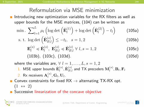
8 September, 2015 Coordinated Multiantenna Interference Management in 5G Networks 144
Reformulation via MSE minimizationIntroducing new optimization variables for the RX filters as well asupper bounds for the MSE matrices, (104) can be written as
min .∑L
l=1µl
(log det
(E
(1)l
)+ log det
(E
(2)l
)− tl
)(105a)
s. t. log det(E
(s)B,l
)≤ −tl, s = 1, 2 (105b)
E(s)l 4 E
(s)l , E
(s)B,l 4 E
(s)B,l ∀ l, s = 1, 2 (105c)
(103b), (103c), (103d). (105d)
where the variables are, ∀ l = 1, . . . , L, s = 1, 2
1. MSE upper bounds E(s)l , E
(s)B,l and TX precoders M
(s)l ,Bl,Fl
2. Rx receivers A(s)l ,Gl,Ul.
Convex constraints for fixed RX → alternating TX-RX opt.(1 ↔ 2)
Successive linearization of the concave objective
c©Antti Tolli, Department of Comm. Engineering

8 September, 2015 Coordinated Multiantenna Interference Management in 5G Networks 145
Mode selection via overloadingInitial allocation
UL slot (1)
DL slot (2)
Final allocation after convergence:
UL slot (1)
DL slot (2)
c©Antti Tolli, Department of Comm. Engineering

8 September, 2015 Coordinated Multiantenna Interference Management in 5G Networks 146
Numerical ExamplesL = 4 D2D pairs, each with 2 antennasBS is equipped with 8 antennasFrequency flat Rician fading with factor κ
[A. Tolli, J. Kaleva and P. Komulainen, ”Mode Selection and Transceiver Design for Rate Maximization in Underlay D2DMIMO Systems”, IEEE ICC, London, UK, June, 2015]
c©Antti Tolli, Department of Comm. Engineering
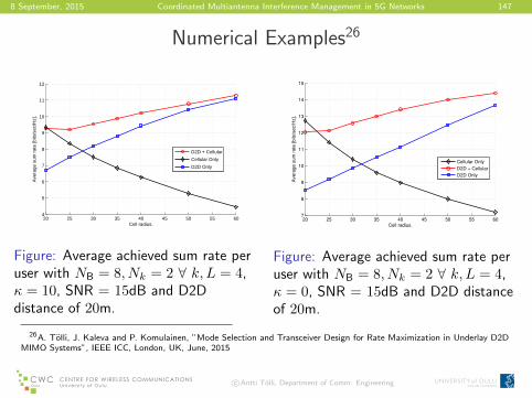
8 September, 2015 Coordinated Multiantenna Interference Management in 5G Networks 147
Numerical Examples26
20 25 30 35 40 45 50 55 604
5
6
7
8
9
10
11
12
Ave
rage
sum
rat
e [b
its/s
ec/H
z].
Cell radius.
D2D + Cellular
Cellular Only
D2D Only
Figure: Average achieved sum rate peruser with NB = 8, Nk = 2 ∀ k, L = 4,κ = 10, SNR = 15dB and D2Ddistance of 20m.
20 25 30 35 40 45 50 55 607
8
9
10
11
12
13
14
15
Ave
rag
e s
um
ra
te [
bits/s
ec/H
z].
Cell radius.
Cellular Only
D2D + Cellular
D2D Only
Figure: Average achieved sum rate peruser with NB = 8, Nk = 2 ∀ k, L = 4,κ = 0, SNR = 15dB and D2D distanceof 20m.
26A. Tolli, J. Kaleva and P. Komulainen, ”Mode Selection and Transceiver Design for Rate Maximization in Underlay D2DMIMO Systems”, IEEE ICC, London, UK, June, 2015
c©Antti Tolli, Department of Comm. Engineering