Embed Size (px)
Citation preview
i
MALIHEH SOLEIMANI
FEASIBILITY STUDY OF MULTIANTENNA TRANSMITTER
BASEBAND PROCESSING ON CUSTOMIZED PROCESSOR
CORE IN WIRELESS LOCAL AREA DEVICES
Master’s thesis
Examiner: Professors Mikko Valkama and Jarmo Takala Examiner and topic approved by the Faculty Council of the Faculty of Computing and Electrical Engineering on 8 November 2013.

ii
ABSTRACT
TAMPERE UNIVERSITY OF TECHNOLOGY Degree Programme in Electrical Engineering SOLEIMANI, MALIHEH: Feasibility Study of Multiantenna Transmitter Base-
band Processing on Customized Processor Core in Wireless Local Area Devic-es Master of Science Thesis, 62 pages, 1 Appendix page January 2013 Major subject: Wireless Communication Circuits and Systems Examiner: Professors Mikko Valkama and Jarmo Takala Keywords: Wireless Local Area Network, Baseband Processing, Parallel Processing,
Physical Layer, Software Defined Radio, Vector Processor.
The world of wireless communications is governed by a wide variety of the standards,
each tailored to its specific applications and targets. The IEEE802.11 family is one of
those standards which is specifically created and maintained by IEEE committee to im-
plement the Wireless Local Area Network (WLAN) communication. By notably rapid
growth of devices which exploit the WLAN technology and increasing demand for rich
multimedia functionalities and broad Internet access, the WLAN technology should be
necessarily enhanced to support the required specifications. In this regard,
IEEE802.11ac, the latest amendment of the WLAN technology, was released which is
taking advantage of the previous draft versions while benefiting from certain changes
especially to the PHY layer to satisfy the promised requirements.
This thesis evaluates the feasibility of software-based implementation for the MIMO
transmitter baseband processing conforming to the IEEE802.11ac standard on a DSP
core with vector extensions. The transmitter is implemented in four different transmis-
sion scenarios which include 2x2 and 4x4 MIMO configurations, yielding beyond
1Gbps transmit bit rate. The implementation is done for the frequency-domain pro-
cessing and real-time operation has been achieved when running at a clock fre-
quency of 500MHz.
The developed software solution is evaluated by profiling and analysing the imple-
mentation using the tools provided by the vendor. We have presented the results with
regards to number of clock cycles, power and energy consumption, and memory usage.
The performance analysis shows that the SDR based implementation provides improved
flexibility and reduced design effort compared to conventional approaches while main-
taining power consumption close to fixed-function hardware solutions.

iii
Preface
The research leading to this Master of Science Thesis was carried out within the Parallel
Acceleration (ParallaX) project, funded by the Finnish Funding Agency for Technology
and Innovation (Tekes). The work was also supported by Broadcom Corporation (earlier
Renesas Mobile). The research work was carried out during the year 2013 at the De-
partment of Electronics and Communications Engineering, Tampere University of
Technology, Tampere, Finland.
I would like to thank my supervisor Prof. Mikko Valkama for the given opportunity
and his enthusiastic support and guidance during this research. It was a great pleasure
for me to work under his supervision and I had this opportunity to learn a lot from him.
I would also like to thank Prof. Jarmo Takala for his valuable guidance and advices
through this research. I would like to extend my gratitude to my friends, M.Sc. Lasse
Lehtonen and M.Sc. Mona Aghababaeetafreshi for sharing their works and experiences
on this research. I am also thankful to Juho Pirskanen, Hannu Talvitie and Ekaterina
Pogosova from Broadcom Corporation for sharing their knowledge.
I would like to express my warmest thanks to my husband, Hossein Saghlatoon, for
his patience, endless support and advices given through all the ups and downs of my
studies.
I would like to extend my appreciation to my brother, Dr. Mohammad Reza
Soleymaani for his constant support, guidance and advices during all years of my stud-
ies.
Finally, I would like to express my utmost gratitude and respect to my beloved fami-
ly, especially my mother to whom I owe whatever I have achieved, for her unlimited
love, invaluable support and encouragement in every possible way she could.
Tampere, December 2013
Maliheh Soleimani

iv
TABLE OF CONTENTS
TERMS AND DEFINITIONS ..................................................................................... vi
1. INTRODUCTION ................................................................................................ 1
1.1. Background and Motivation .......................................................................... 1
1.2. Scope of the Thesis ........................................................................................ 3
1.3. Outline of the Thesis ..................................................................................... 3
2. IEEE802.11ac STANDARD ................................................................................. 5
2.1. Overview of the IEEE802.11 Standards ......................................................... 5
2.2. IEEE802.11 Physical Layer Architecture ....................................................... 6
2.2.1. Physical Layer Convergence Protocol ............................................... 6
2.2.2. Physical Medium Dependent ............................................................ 8
2.3. IEEE802.11 Medium Access Control Specifications ...................................... 8
2.3.1. Carrier Sensing Mechanisms............................................................. 8
2.3.2. Distributed Coordination Function .................................................... 9
2.3.3. Point Coordination Function ............................................................. 9
2.4. An Overview of IEEE802.11a ..................................................................... 10
2.5. High Throughput Specifications .................................................................. 10
2.5.1. High Throughput Physical Layer .................................................... 10
2.5.2. High Throughput Medium Access Control ...................................... 12
2.6. Overview of IEEE802.11ac Standard ........................................................... 12
2.7. Very High Throughput Physical Layer Specifications .................................. 13
2.7.1. Channelization ................................................................................ 14
2.7.2. Modulation and Coding Scheme ..................................................... 15
2.7.3. MIMO Operation ............................................................................ 16
2.8. Very High Throughput Medium Access Control Specifications ................... 16
2.8.1. Frame Aggregation ......................................................................... 16
2.8.2. Block Acknowledgement ................................................................ 17
2.8.3. Power Saving Enhancement ............................................................ 17
3. PROGRAMMABLE SOFTWARE DEFINED RADIO ....................................... 18
3.1. Introduction ................................................................................................. 18
3.2. Real-Time Requirement ............................................................................... 19
3.3. Very Long Instruction Word ........................................................................ 20
3.4. Vector Processing ........................................................................................ 21
3.4.1. Vector Processing Units .................................................................. 21
3.4.2. Pros and Cons ................................................................................. 21
3.4.3. Main Operations ............................................................................. 23
3.4.4. Optimization Schemes .................................................................... 23
3.4.5. Power Consumption ....................................................................... 24
3.5. Single Instruction Multiple Data .................................................................. 24
3.6. Vector Processors Deployment in Baseband Processing Wireless Modems .. 25
v
3.7. ConnX BBE32 DSP Core ............................................................................ 26
4. IEEE802.11ac TRANSMITTER IMPLEMENTATION ...................................... 29
4.1. Data Structure.............................................................................................. 29
4.1.1. Legacy Preamble ............................................................................ 30
4.1.2. Very High Throughput Preamble ................................................... 31
4.1.3. VHT Data Field .............................................................................. 32
4.1.3.1. Stream Parser.................................................................................. 32
4.1.3.2. Constellation Mapper...................................................................... 33
4.1.3.3. Low-Density Parity Check Tone Mapper ........................................ 33
4.1.3.4. Space Time Block Coding .............................................................. 34
4.1.3.5. Pilot Insertion ................................................................................. 35
4.1.3.6. Cyclic Shift Diversity ..................................................................... 35
4.1.3.7. Spatial Mapping ............................................................................. 36
4.1.3.8. Phase Rotation ................................................................................ 36
4.2. Transmission Scenarios ............................................................................... 36
4.2.1. Case a: 2x2 SU-MIMO Transmission................................................. 36
4.2.2. Case b: 4x4 SU-MIMO Transmission ................................................ 38
4.2.3. Case c: 2x2 Antenna Configuration with 1x1 SU-SISO Transmission 39
4.2.4. Case d: 4x4 Antenna Configuration with 2x2 SU-SISO Transmission 40
4.3. Time and Frequency Parameters .................................................................. 41
5. RESULTS AND ANALYSIS .............................................................................. 42
5.1. Software Implementation ............................................................................. 42
5.2. Clock Cycles ............................................................................................... 42
5.3. Power Consumption .................................................................................... 44
5.4. Energy per Bit ............................................................................................. 48
5.5. Memory Usage ............................................................................................ 50
5.6. Analysis ...................................................................................................... 51
5.7. Related Works ............................................................................................. 52
6. CONCLUSION ................................................................................................... 54
REFERENCES ........................................................................................................... 56
APPENDIX 1: CLOCK CYCLE RESULTS ............................................................... 61

vi
TERMS AND DEFINITIONS
ACK Acknowledgement
ALU Arithmetic Logic Units
AP Access Point
ASIC Application Specific Integrated Circuit
BCC Binary Convolutional Coding
BPSK Binary Phase Shift Keying
CSD Cyclic Shift Diversity
CSMA/CA Carrier Sense Multiple Access/Collision Avoidance
CSMA/CD Carrier Sense Multiple Access/Collision Detection
CTS Clear-To-Send
DCF Distributed Coordination Function
DL Downlink
DSP Digital Signal Processor
FFT Fast Fourier Transform
FPGA Field Programmable Gate Array
GI Guard Interval
GPP General Purpose Processor
GSM Global System for Mobile Communications
HT High Throughput
IEEE Institute of Electrical and Electronics Engineers
LDPC Low Density Parity Check
MAC Medium Access Control
MCS Modulation and Coding Scheme
MIMO Multiple-Input Multiple-Output
MPDU MAC Protocol Data Unit
MU Multiple User
OFDM Orthogonal Frequency Division Multiplexing
OSI Open Systems Interconnection
PCF Point Coordination Function
PHY Physical Layer
PLCP Physical Layer Convergence Protocol
PMD Physical Medium Dependent
QAM Quadrature Amplitude Modulation
RTS Request-To-Send
SAP Service Access Point
SDR Software Defined Radio
SIMD Single Instruction Multiple Data
STA Station
SNR Signal to Noise Ratio
STBC Space Time Block Coding

vii
VHT Very High Throughput
VLIW Very Long Instruction Word
VLSI Very Large Scale Integration
Wi-Fi Any WLAN products which is based on IEEE802.11 stand-
ard
WLAN Wireless Local Area Networks
1
1. INTRODUCTION
In this chapter, the history of the wireless communications and Wireless Local Area
Networks will be reviewed. Furthermore, the motivation and scope of the thesis will be
described. In the final part, the rest of thesis will be outlined.
1.1. Background and Motivation
Wireless communications has always been a part of people’s lives throughout the ages.
Starting from simple speech to fire and smoke, humankind has been always trying to
invent different ways to communicate over long distances. In the beginning of 19th
cen-
tury, with the help of science, more sophisticated communication methods were devel-
oped e.g. telegraph.
In the end of 19th century, the wired communications era was revolutionized by in-
venting telephone. Although, wired communications systems provide reliable, high in-
formation transmission rate over long distances, it always suffers from the limitation by
wires. That limitation makes the idea of wireless communications more attractive. At
first, because of the costs and complexity of electronics devices, the wireless/radio
communication was mainly used in the military and broadcasting applications. Then, in
the beginning of the 1990s, the first digital cellular networks working on Global System
for Mobile Communications (GSM) were built. After that, the extremely increasing rate
of mobile devices led to widespread use of mobile in the developed and developing
countries.
However, wireless communication is one of the most vibrant areas in the communi-
cations field. Since the 1960’s when the wireless communications became as an area of
research interest and wired communications found limited, it has been exposed by a
surge of improvements, research activities, and novelties. During the recent years, this
field has been considerably developed due to several factors. First of all, explosive
growth in the number of users whose demand for seamless service/connection has
changed the wireless communication and even introduced new objectives. Besides, the
intense progressive trend of the VLSI technology has allowed more complex systems to
be integrated on a silicon chip. Meanwhile, the sophisticated signal processing methods
have been supported by the fairly developed VLSI architectures to implement the novel
algorithms in low power and low cost techniques [1, 2].
As the wireless communications systems have been increasingly involved into the
many aspects of our daily lives, they have experienced much faster improvement rather
than the rest of communications science. Furthermore, in the recent years, the word
PORTABLE has introduced new features into the communication fields and devices.

2
Obviously, the conventional wired communication networks were not able to provide
the connection along the mobility; therefore, the Wireless Local Area Network
(WLAN)/Wi-Fi protocol was invented which was the sole practical solution to wireless
connectivity in indoor environments.
For the first time, in 1997, the Institute of Electrical and Electronics Engineering
(IEEE) introduced a new family of the communication standards titled IEEE802.11 for
the WLAN systems. Due to the rapid growth and popularity of the wireless handheld
devices, the wireless communication standards have been extremely developed during
the past decade. However, more reliable, low power, low cost connections are also seen
as crucial aspects to be supported by the WLAN standards.
Until now, the WLAN standard has substantially changed as new theory and imple-
mentation methods evolved; therefore several amendments have been released to correct
or extend the previous versions such as IEEE802.11a and 802.11b. Essentially, the
IEEE802.11 standards are described based on Physical (PHY) and Medium Access
Control (MAC) layers. The MAC layer provides the functionalities to allow reliable
data transmission, whereas the PHY features are used to govern the transmission and
reception procedure [3].
Nowadays, a widespread application of the WLAN devices in the everyday life is
witnessed; moreover, the increasing demand for higher speed connection and data
throughput results in the new version of the IEEE802.11 called 802.11ac whose PHY
and MAC features enhanced the throughput up to 6Gbps. It is worth mentioning that the
most part of this improvement is made by the PHY features which are also the main
focus of this study [4].
The IEEE802.11ac amendment actually overcame the limitations in the previous
standards. The employment of wider bandwidth, Multiple-Input Multiple-Output
(MIMO) transmission, higher number of spatial streams, and greater modulation size all
together delivered the next leap in the performance of the Wi-Fi technology.
Another side of the wireless communications world is user equipment, such as mo-
bile devices and modems which are also evolving, in their turn, in different features and
functionalities. A clear majority of the current wireless devices are based on the imple-
mentation of the baseband digital signal processing algorithms in the Application Spe-
cific Integrated Circuits (ASIC) [5]. Although ASIC circuits allow sufficiently fast pro-
cessing, they are fixed function which means they are not reconfigurable. On the other
hand, as the number of communication standards and implementation algorithms con-
tinue to grow, the hardware implementations techniques moderately suffer from the lack
of adaptability and compatibility to the new technologies. Particularly, the conventional
modem designs are implemented in the silicon/semiconductor technology. With a new
release, the previous designs are not mostly worth to be redesigned to accommodate the
new specifications, as they would need expensive and time consuming procedures.
Therefore a revolutionary method called Software Defined radio (SDR) technology in-
troduced whose components that have been typically implemented in hardware are in-
stead implemented using embedded devices or DSP cores. In fact, SDR aims to address

3
the fixed-function implementation difficulties by exchanging the fixed hardware im-
plementation with a fully programmable platform [6, 7]. This programma-
ble/configurable platform could be General Purpose Processor (GPP), Field Program-
mable Gate Array (FPGA), Digital Signal Processor (DSP), or any combination of
them.
Software Defined Radio PHY layer wireless modems can be considered as the new
trend in the field of wireless communications. In contrast with the dedicated hardware,
the software based implementation can be easily modified to implement a wide variety
of standards on the same platform. The usage of the software based solution results in
flexibility, ease of design, time-to-market, and cost savings due to use of a single plat-
form. However, the main concern is obtaining sufficient performance which can be
achieved by having parallelism in the configurable platforms. The next issue is the en-
ergy efficiency in the fixed-function solutions which is not vincible by programmable
SDR, thus the main aim is to improve the energy efficiency of the SDR solutions as
close as the fixed-function methods. Although SDR solution would not reach the ideal
case, if the gap is rational, then the cost savings in design will make the SDR solution
desirable. Basically, making vector parallelism explicit in the programming is the key
requirements of the SDR solution [8].
1.2. Scope of the Thesis
In this thesis, the feasibility of software based implementation using Very Long Instruc-
tion Word (VLIW) processor for the real-time operation of IEEE802.11ac transmitter
full PHY layer baseband processing in four different transmission scenarios which in-
clude 2x2 and 4x4 MIMO configurations is addressed. As the processing platform,
stemming from the requirements for very fast processing of huge amounts of data with
transmission bit rates in the order of 1Gbps, the customized VLIW processor with vec-
tor processing capabilities is used. Such a software based implementation, if found fea-
sible, can offer highly improved flexibility, much faster time-to-market, and highly im-
proved possibilities to bringing in new transmission features and enhancements. In this
project, the software development has been collaborative effort which leads to such an
implementation capable of providing a huge part of the IEEE802.11ac requirements.
In the existing literature, a clear majority of the WLAN device implementations are
fixed-function hardware based solutions [9]. In recent reports, some contributions
have also been made towards the software defined radio concept [11]. However, in
some works [11]-[14], only selected parts of PHY or MAC layer are typically targeted
while other processing still relies on dedicated hardware.
1.3. Outline of the Thesis
The rest of thesis is organized as follows:

4
Chapter 2 presents the basics of the IEEE802.11 standards including both PHY and
MAC layers. In the proceeding chapter, the 802.11ac and 802.11n amendments are also
described in details.
Moreover, in Chapter 3, an overview of the vector processor in the various aspects
such as architecture, pros and cons are given. In addition, the employed processor and
some of its main features are also described.
In Chapter 4, a detailed description of the selected transmission scenarios of
IEEE802.11ac standard is given. Furthermore, the software development environment
and some of the employed optimization approaches are introduced.
The implementation results and analysis of the transmitter in the terms of power and
energy consumption, clock cycle and memory usage are then provided in Chapter 5.
Finally, Chapter 6 appends some concluding remarks to the thesis. In addition, the fu-
ture status of the project will be also stated.

5 5
2. IEEE802.11AC STANDARD
In this chapter, all the Wireless Local Area Network (WLAN) standards belonging to
the IEEE802.11 family will be reviewed. The general Physical (PHY) and Medium Ac-
cess Control (MAC) layers features of this family are also described. The main dis-
cussed standard is the latest released called IEEE802.11ac, which is also referred to as
the Very High Throughput (VHT); all the features related to these standards are also
presented.
2.1. Overview of the IEEE802.11 Standards
The history of the IEEE802.11 standard dates back to 1997, when IEEE released the
first wireless networking standard, the IEEE802.11 WLAN standard [15]. As it can be
realized from its name, it belongs to the popular group of the IEEE802.x standards, such
as IEEE802.3 standard for Ethernet and IEEE802.15 for Wireless Personal Area net-
works (WPANs) [16]. In fact, it can be said that IEEE802.11 WLAN specification was
written to extend the functionality provided by 802.3 Wired LAN standard [17]. The
IEEE 802.11 standard determines a set of Physical layer and Medium Access Control
specifications to implement the WLANs communication systems in different frequency
bands [18, 19]. Basically, until 1997, the major constraint for spreading the WLAN
technology was the low penetration of the devices working based on the wireless tech-
nology. Since the popularity of wireless devices such as laptops and cell phones has
increasingly risen, the number of users who want to access the internet not only in their
offices but also in the other locations like restaurants, airport and shopping centers has
also risen up, significantly. As a result, the WLAN technology has to be updated to ful-
fill the increasing demand for WLAN connection.
The IEEE802.11 was the basic version of the WLANs communication systems;
therefore different amendments were released to extend or correct the previous specifi-
cations. The first released version of the WLAN standard family was IEEE 802.11a, but
the first broadly accepted version was IEEE 802.11b (July 1999) which used the
2.4GHz frequency with 20MHz bandwidth and provided up to 11Mbps data rate. Until
2003, the main wireless protocol was IEEE 802.11b, but in order to achieve higher data
rate another version was presented and authorized named IEEE 802.11g. From the oper-
ation frequency, bandwidth and number of spatial streams point of views, the IEEE
802.11b and 802.11g standards were similar, but IEEE 802.11g was using a new modu-
lation scheme, namely, Orthogonal Frequency Division Multiplexing (OFDM), which
resulted in up to 54 Mbps data rate. It was also compatible to IEEE802.11b, which was
a novel feature in that time.
2. IEEE802.11AC STANDARD 6
Then in 2009, the IEEE committee introduced and rectified a new version of WLAN
standard, called IEEE802.11n, which brought new concepts into the wireless communi-
cations world. For the first time, the MIMO concept was exploited, which provided up
to 600Mbps. This standard supports the usage of up to four spatial streams or 4x4
MIMO transmission system within two different channel bandwidths, 20 and 40MHz
[20]. It is worth mentioning that IEEE802.11n is the version which has brought new
format of the PHY layer, called High Throughput (HT), which will be discussed in sec-
tion 2.4.
As mentioned earlier, the IEEE802.11 standard is a set of PHY and MAC specifica-
tions to support the wireless network. The PHY selects the appropriate modulation
scheme with respect to the channel conditions given and provides the bandwidth; how-
ever the MAC layer governs how the available bandwidth shall be shared among all the
wireless stations (STAs) [21]. Although several versions have been released to develop
the protocol, the original MAC remained intact. It means that all the technology im-
provement evolved with the help of new PHY features such as the modulation and cod-
ing schemes, MIMO transmission concept, wider channel bandwidth and so on.
2.2. IEEE802.11 Physical Layer Architecture
The IEEE802.11 Physical layer is basically an interface between the medium access and
the MAC layer, as depicted in Figure 1. It also defines the radio wave modulation and
signalling characteristics for data transmission. Fundamentally, the 802.11 PHY layer
consists of two generic functions, Physical layer Convergence Protocol (PLCP) and
Physical Medium Dependent (PMD). Both functions will be discussed in the following.
In general, the physical layer can be divided into five categories, which define different
transmission techniques [22, 23]:
Frequency Hopping Spread Spectrum (FHSS)
Direct Sequence Spread Spectrum (DSSS)
Infrared light (IR)
High Rate Direct Sequence (HR/DS)
Orthogonal Frequency Division Multiplexing (OFDM)
Each PHY layer has specific PLCP and PMD to control the transmission and recep-
tion procedure [24].
2.2.1. Physical Layer Convergence Protocol
Physical Layer Convergence Protocol (PLCP) determines a suitable mapping method
for IEEE802.11 MAC Protocol Data Units (MPDUs) into a framing format appropriate
for sending and receiving user data and information management among two or more
STAs using the associate PMD system. [18]
2. IEEE802.11AC STANDARD 7
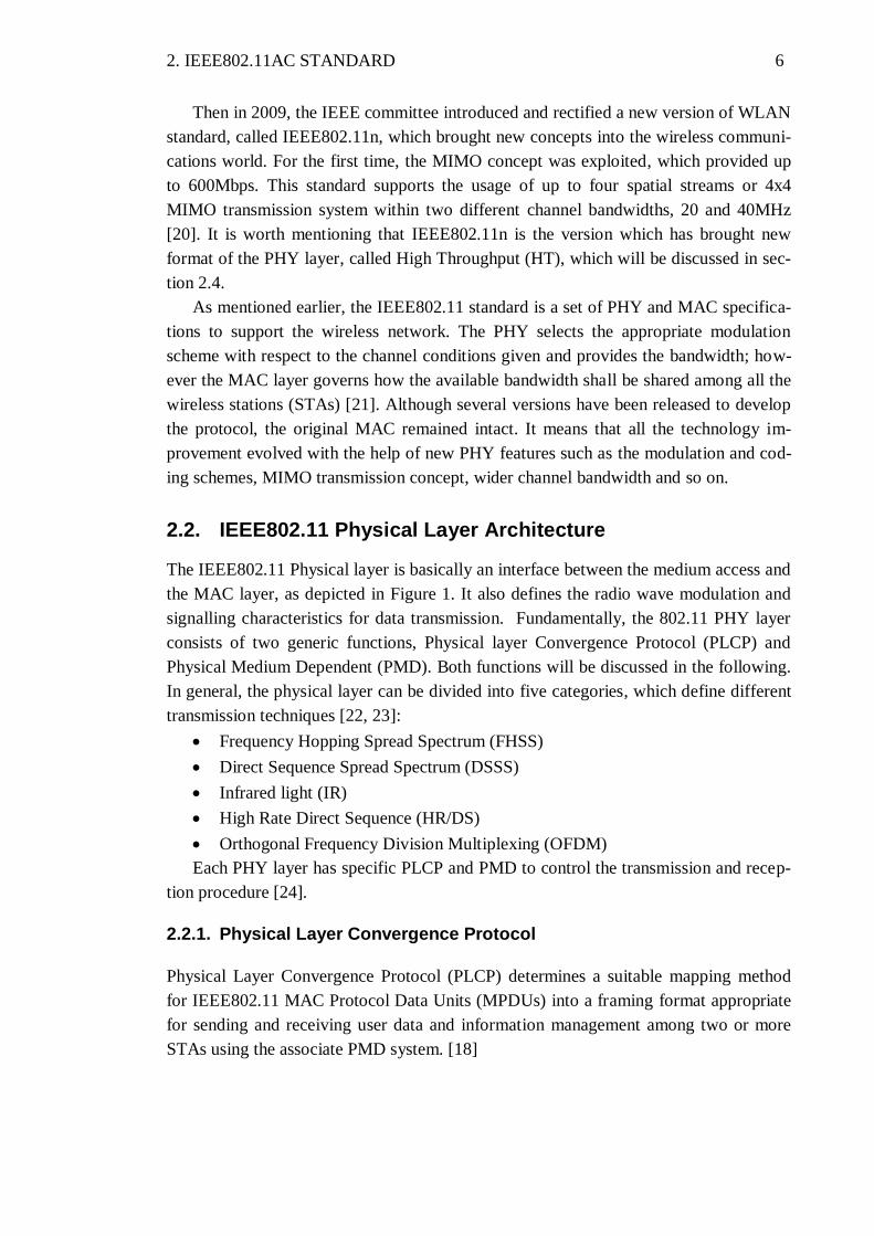
Figure 1. PHY and MAC sub-layers structure
Figure 1, illustrates how the data link and physical layers are connected to each oth-
er. According to Figure 1, the MAC sub-layer communicates with the PLCP through
Physical Layer Service Access Point (PHY_SAP) by using a set of instructive com-
mands or fundamental instructions. Basically, when the MAC layer commands the
PLCP to operate, it prepares the MPDUs for the transmission. It is worth observing that
the PLCP minimizes the MAC layer dependency on the PMD sub-layer by mapping the
MPDUs into a suitable format for transmission. It also delivers the incoming frames
from the wireless medium to the MAC layer.
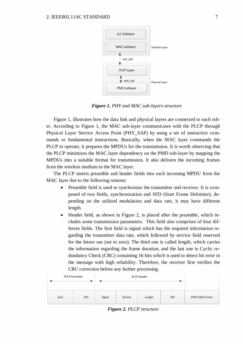
The PLCP inserts preamble and header fields into each incoming MPDU from the
MAC layer due to the following reasons:
Preamble field is used to synchronize the transmitter and receiver. It is com-
posed of two fields, synchronization and SFD (Start Frame Delimiter), de-
pending on the utilized modulation and data rate, it may have different
length.
Header field, as shown in Figure 2, is placed after the preamble, which in-
cludes some transmission parameters. This field also comprises of four dif-
ferent fields. The first field is signal which has the required information re-
garding the transmitter data rate, which followed by service field reserved
for the future use (set to zero). The third one is called length, which carries
the information regarding the frame duration, and the last one is Cyclic re-
dundancy Check (CRC) containing 16 bits which is used to detect bit error in
the message with high reliability. Therefore, the receiver first verifies the
CRC correction before any further processing.
Sync SFD Signal Service Length CRC PPDU-MAC frame
PLCP Preamble PLCP Header
Figure 2. PLCP structure
LLC Sublayer
MAC Sublayer
PMS Sublayer
PLCP Layer
Datalink Layer
Physical Layer
PHY_SAP
PMS_SAP
2. IEEE802.11AC STANDARD 8
In the end, the resulted frame (the MPDU and the additional preamble and header) is
referred to as PLCP Protocol Data Unit (PPDU) [24].
2.2.2. Physical Medium Dependent
With reference to the provided definition for the PLCP, the Physical medium Dependent
defines the data transmission and reception techniques between STAs and PHY entities
through the wireless medium, including modulation and demodulation and hiving inter-
ference with air medium [25]. As it can be observed in Figure 1, PLCP and PMD com-
municate through the PMD_SAP to control the transmission and reception functions
[24].
2.3. IEEE802.11 Medium Access Control Specifications
The Medium Access Control (MAC) layer is one of the sublayers of the data link layer
in the Open Systems Interconnection (OSI) model. Principally, the MAC layer is a set
of rules to determine how to access the medium and data link components, but the most
important functionality of the MAC layer is addressing and channel access control that
makes the communication of the multiple stations possible.
The key point is that the IEEE802.11 MAC layer is compatible with the Ethernet
standard (IEEE802.3) at the link layer, that compatibility is resulted from the fact that
these two standards are similar in terms of addressing and channel access [26]. It shall
be also added that the Carrier Sense Multiple Access technique (CSMA) is also sup-
ported by IEEE802.11 MAC layer which makes the access to the shared wireless medi-
um feasible [27]. According to CSMA technique, the STA is allowed to transmit when
the channel is ‘idle’; otherwise it has to postpone its transmission [28].
The MAC layer architecture supports two different fundamental access methods, the
Distributed Coordination Function (DCF) and the Point Coordination Function (PCF).
Besides these two key functions, the Hybrid Coordination Function (HCF), the Mesh
Coordination Function (MCF), and their coexistence are included in the IEEE802.11
WLAN standard [29]. The simple distributed, contention based access protocol support-
ed by CSMA/CA technique is the basic MAC protocol for IEEE802.11 [28].
2.3.1. Carrier Sensing Mechanisms
Except the time when the STA is transmitting and therefore knowing that the medium is
busy, it requires an additional mechanism to check the state of channel. Carrier Sensing
methods are used (by STAs) to determine whether the medium is busy or not. In the
standard, two main carrier sensing mechanisms are defined, namely, Physical Carrier
Sensing (PCS), which is supported by PHY layers, and Virtual Carrier Sensing (VCS)
[30]. However, a third carrier sensing method is also used called Network Allocation

2. IEEE802.11AC STANDARD 9
Vector (NAV) provided by MAC specifications. The state of medium will be deter-
mined by using either PCS or VCS [31].
The PCS technique must be provided by the PHY layers. In fact, the PCS is an ob-
ligatory carrier sensing method in any PHY layer to state the medium status; the respon-
sible function for this purpose is called Clear Channel Assessment (CCA). In this meth-
od, the channel state can be determined by using the PLCP layer, if it indicates that the
channel is ‘Idle’, the transmission procedure can be initiated. The busy indication
should be raised when another signal is detected in the medium; in this case, the station
would enter a contention window and the transmission is delayed until the end of the
impending transmission.
The VCS technique ascertains the state of medium by spreading the reservation in-
formation announcing the usage of medium. For instance, the transmission and recep-
tion of the Request-To-Send (RTS) and Clear-To-Send (CTS) frames (which happens
before the actual data transmission) is an example of distributing the reservation infor-
mation to the medium [32]. When a node has a packet to transmit, it first ensures that no
other node is transmitting by sending the RTS frame. When the receiving station is
ready to receive the data, it responds by sending a CTS frame. Once the RTS/CTS ex-
change is complete, the transmitter node can transmit its data frame without any concern
regarding the interference or any other problem. The medium is definitely idle and re-
served during a certain period of time which is defined by RTS and CTS frames, in fact
this period is enough to transmit the actual data frame and return the Acknowledgement
frame (ACK). The medium reservation can be done by station which either receives the
RTS or the CTS frames. [18]
2.3.2. Distributed Coordination Function
The DCF is the fundamental access method in the IEEE802.11 MAC layer which is
used to support asynchronous data transfer on a best effort basis [33]. DCF provides
distributed, but coordinated access in such a way that only one station can transmit [26].
In fact, in the case that the medium is not sensed to be busy, the transmission may pro-
ceed; otherwise it may be deferred. Therefore, the presence of the DCF is mandatory in
all types of station [34]. It is also known a Carrier Sense Multiple Access with Collision
Avoidance (CSMA/CA). The Carrier Sense Multiple Access with Collision Detection
(CSMA/CD) has not been used due to the fact that STA is not capable to listen to the
channel while transmitting.
2.3.3. Point Coordination Function
The PCF access method is an optional technique which is only applicable in the infra-
structure network configurations. In this method, one Point Coordinator (PC) is required
to determine which station will transmit. Basically, this operation is done based on the
polling mechanism and the PC is playing the role of the polling master. It can be said

2. IEEE802.11AC STANDARD 10
that the PCF is a contention free service provider, which has some special service points
to assure the provided medium is without contention [18, 35].
2.4. An Overview of IEEE802.11a
The latest two popular versions of the WLAN standards, including IEEE802.11n and
IEEE802.11ac, entail the fundamental PHY and MAC specifications of the
IEEE802.11a. Consequently, the key and common specifications of the 802.11a will be
discussed.
In 1999, the IEEE released the first established WLAN standard, IEEE802.11a
which was designed to operate in the 5GHz frequency range within a 20MHz channel
bandwidth divided into 64 subbands. The 802.11a is a packet based radio interface and
uses an OFDM based encoding scheme rather than FHSS or DSSS to send the data. Ac-
cordingly, the assigned bandwidth is channelized in such a way that 48 subcarriers out
of 64 are used for data transmission, 4 subcarriers are used as pilot, and the rest are null.
The subcarriers design was based on FFT size of 64, as shown in Figure 3. Based on the
allocated PHY specifications, the IEEE802.11a standard was expected to support up to
54Mbps for business and office applications, but it was suffering from the limited cov-
erage range, delayed time-to-market and high cost.
The 802.11a MAC unit works based on the Carrier Sense Multiple Access, Collision
Avoidance (CSMA/CA) in which the transmitter listens to figure out the status of the
medium either busy or idle. In the medium is idle, the transmitter sends a short Request-
To-Send (RTS) package containing the information regarding the package. Then, the
transmitter waits for the response from the receiver before starting the transmission.
Meanwhile, other transmitters within the reach area also receive the RTS package which
helps them to estimate how long the transmission will take.
2.5. High Throughput Specifications
The IEEE802.11n standard is the High Throughput amendment to the 802.11 standard.
The key features of the 802.11n are the application of MIMO and OFDM concepts
which lead to significant increase in the data rate in 40MHz channel bandwidth. With
the aid of these two techniques, the data rate of 600Mbps was obtained. [20]
Regarding the High Throughput IEEE802.11 standard, two groups of specifications
will be discussed. The first one is the PHY specifications, and the second is MAC.
2.5.1. High Throughput Physical Layer
The HT PHY is based on the Orthogonal Frequency Division Multiplexing (OFDM)
which is well suited for the wideband systems in the frequency selective environment.
In addition, OFDM is bandwidth efficient as multiple data symbols can be transmitted
on different orthogonal frequencies or subcarriers, simultaneously. Therefore, the
OFDM provides better spectral efficiency and immunity to multipath fading. [36]
2. IEEE802.11AC STANDARD 11
In the HT PHY, in order to modulate the data subcarriers, Binary Phase Shift Key-
ing (BPSK), Quadrature Phase Shift Keying (QPSK), 16-Quadrature Amplitude Modu-
lation (16-QAM) and 64-Quadrature Amplitude Modulation (64-QAM) are used as the
modulation scheme. The Forward Error Correction (FEC) or the convolutional coding
technique is deployed with the coding rate of 1/2, 2/3, 3/4, or 5/6. As an optional fea-
ture, the Low-Density Parity-Check (LDPC) coding method can be also used. These
features are known as Modulation and Coding Scheme (MCS) to define the modulation
size and coding rate. The notable point regarding the MCS definition in the 802.11n is
that it also determines the number of spatial streams. It means that MCS parameters
include modulation, coding rate and spatial stream number which bring complexity in
MCS set selection. [28]
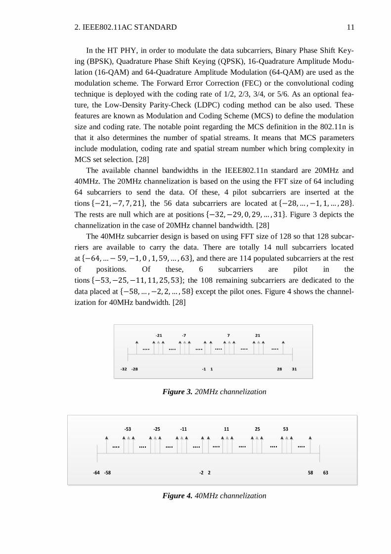
The available channel bandwidths in the IEEE802.11n standard are 20MHz and
40MHz. The 20MHz channelization is based on the using the FFT size of 64 including
64 subcarriers to send the data. Of these, 4 pilot subcarriers are inserted at the
tions { }, the 56 data subcarriers are located at { }.
The rests are null which are at positions { }. Figure 3 depicts the
channelization in the case of 20MHz channel bandwidth. [28]
The 40MHz subcarrier design is based on using FFT size of 128 so that 128 subcar-
riers are available to carry the data. There are totally 14 null subcarriers located
at { }, and there are 114 populated subcarriers at the rest
of positions. Of these, 6 subcarriers are pilot in the
tions { }; the 108 remaining subcarriers are dedicated to the
data placed at { } except the pilot ones. Figure 4 shows the channel-
ization for 40MHz bandwidth. [28]
Figure 3. 20MHz channelization
Figure 4. 40MHz channelization
…. …. …. …. …. …. …. ….
-64 -58 -2 2 58 63
-53 -25 -11 11 25 53
…. …. …. …. …. ….
-32 -28 -1 1 28 31
-21 -7 7 21

2. IEEE802.11AC STANDARD 12
It is worth pointing out that there are some other optional features such as Space
Time Block Coding (STBC) scheme, 400ns Guard interval (GI) and beam forming
which are applicable at both transmission and reception sides. With the help of these
PHY features, a maximum data rate of 600Mbps is available in the 802.11n standard.
The HT PHY includes two main functional entities, namely, the PLCP and PMD
functions which are similar to the basic model for the 802.11 standard, explained in sec-
tion 2.2.
2.5.2. High Throughput Medium Access Control
Although, it was found that without any enhancement in the MAC layer, the end user
would benefit from the PHY layer improvement. Therefore, the HT MAC layer is al-
most same as the original one, but still some enhancement has been made to improve
the efficiency in the form of frame aggregation and block acknowledgement [31]. Since,
the MAC mechanisms used in the 802.11n are similar to the 802.11ac; these changes
will be discussed in the VHT part, comprehensively.
2.6. Overview of IEEE802.11ac Standard
As the IEEE802.11n amendment became popular and matured enough in the market, in
May 2007 the IEEE committee organized a new study group to investigate the feasibil-
ity of Very High Throughput (VHT) technology. This group released the first draft ver-
sion in 2011 which was capable of providing data rate up to 6.93Gbps, under certain
circumstances. This considerable high data rate is coming from standardized modifica-
tion to both PHY and MAC layers of the IEEE802.11n standard which will be described
in the following sections.
The key requirement of the IEEE802.11ac is the compatibility with the previous
amendments, IEEE802.11a and IEEE802.11n in the frequency band of 5GHz. It must be
noted that the IEEE802.11ac was restricted to the frequency band lower than 6GHz, as
the higher frequency band was dedicated to the next generation of WLAN standard,
called IEEE802.11ad. Although in the 802.11ac standards, both PHY and MAC layers
specification have been changed, the major part of the data rate enhancement is stem-
ming from the new PHY features.
The first generation of the IEEE802.11ac devices must provide at least the previous
PHY requirements of the 802.11n such as up to three spatial streams; moreover they are
also expected to include the 256-QAM modulation. The rest of PHY features like STBC
and LDPC are expected to be employed in the next generations of the 802.11ac devices.
However, the usage of the optional properties results in both throughput and robustness
enhancement of the wireless systems. Figure 5 presents all the mandatory and optional
PHY features for the IEEE802.11ac. The principal transmitter and receiver block dia-
gram in the IEEE802.11ac are also presented in Figure 6 and Figure 7, respectively.
However, main focus of this thesis is on the transmitter chain.

2. IEEE802.11AC STANDARD 13
Figure 5. PHY layer features for IEEE802.11ac
2.7. Very High Throughput Physical Layer Specifications
The main PHY features and enhancements for the IEEE802.11ac standards to increase
the data rate include the wider channel bandwidth, efficient modulation and coding
schemes, higher number of spatial streams and downlink multiuser MIMO (DL MU-
MIMO) transmission.
In the previous amendments, the channel bandwidths of 20MHz and 40 MHz were
used. However, the bandwidth in the 802.11ac was expanded to 80MHz and 160MHz
which improve the data rate, significantly. The capability of using non-contiguous
channels to make wider channel bandwidth and better fit into the available spectrum is
one of the main remarkable features of IEEE802.11ac PHY layers. By this means, two
non-contiguous 80MHz channels can define a 160MHz channel (80+80 MHz). The
IEEE802.11ac standard also exploits the newly defined 256 Quadrature Amplitude
Modulation (QAM) with the different coding rates which considerably increase the data
rate.
Figure 6. Functional transmitter chain
1, 2 Spatial Stream
20, 40, 80 MHz
Basic MIMO/SDM
Convolutional ode
VHT Preamble
2-8 Spatial Streams
160MHz, 80+80MHz
Short GI, 256 QAM
DL MU-MIMO
TxBF
STBC
LDPC Code
Mandatory Optional
Ro
bu
stn
ess
Enh
ance
men
tTh
rou
ghp
ut
Enh
ance
men
t
Add pad bits + service field
ScramblerFEC
encodingStream parser
BCC Interleaver
ModulatorLDPC tone
mapper
Frequency Segment deparser
STBC Encoder
Add pilot carriers
Set Cyclic shifts
Spatial mapping
IFFT+CPPhase
rotation
Set L-STF
Set L-LTF
Generate L-SIG
Generate VHT-SIG-A
Mux Oversampling DAPN
modelingPA
Data bits (possibly extended
with zeros)
Transmitted Signal
Generate DATA field
Generate PPDU/PLCP/PHY preamble
MuxMux
Set VHT-STF
Set VHT-LTF
Generate VHT-SIG-B
MuxMux

2. IEEE802.11AC STANDARD 14
Figure 7. Functional receiver chain
In addition to the channel bandwidth and modulation and coding scheme improve-
ment, the DL MU-MIMO feature is defined in the 802.11ac that allows an Access Point
(AP) to transmit data streams to the multiple users, simultaneously. This feature can be
also discussed in both terms of MAC and PHY layers.
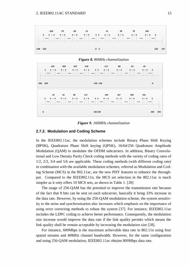
2.7.1. Channelization
The 20MHz and 40MHz channelization for the 802.11ac is similar to the 802.11n
standard, therefore, we only define the design for 80MHz and 160MHz channels. The
80MHz subcarrier design is based on the 256 FFT points meaning that 256 subcarriers
are available to carry the data. The subcarriers indices start from -128 to 127, as depict-
ed in Figure 8. There are 14 null subcarriers which are located at
{ }, and 8 pilot subcarriers which are at positions
{ }. The rest of subcarriers (234 subcarriers) are
data subcarriers placed at { } except those 8 indices which are occu-
pied by the pilot subcarriers. [28]
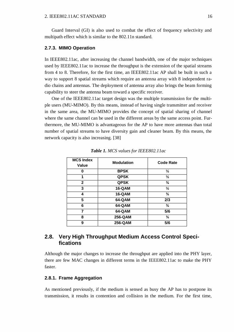
In the case of 160MHz channel, the FFT size is 512 including 28 null subcarriers, 16
pilot subcarriers, and 468 data subcarriers. The 160MHz subcarrier structure is made of
two 80MHz portions, in such a way that the lower and upper 80MHz populated subcar-
riers are mapped to -250 to -6 and 6 to 250, respectively. The null subcarriers are locat-
ed at { }, the 16
pilots are at { }. The remaining sub-
carriers are the data subcarriers. Figure 9 shows the 160MHz channelization [28]. The
new channel bandwidth definition brings more flexibility in the term of channel assign-
ment to avoid any overlap to other channels or even radars.
AGC ADGet frequency
segmentsL-STF + L-LTF
Timing estima
tion
Downsampling
L-STF Frequency estimation
VHT-LTF Timing estimation
L-STF Frequency estimation
Frequency and timing error removal
Remove CP
FFT
LMMSE channel estimator
SINR estimation
Detect L-SIG, VHT-SIG-A, and VHT-SIG-B fields
Detect DATA field
MAC
Time Domain processing
Frequency Domain processing
Add time Delay
Add noise
PN model
Add Freq. offset
2. IEEE802.11AC STANDARD 15
Figure 8. 80MHz channelization
Figure 9. 160MHz channelization
2.7.2. Modulation and Coding Scheme
In the IEEE802.11ac, the modulation schemes include Binary Phase Shift Keying
(BPSK), Quadrature Phase Shift keying (QPSK), 16/64/256 Quadrature Amplitude
Modulation (QAM) to modulate the OFDM subcarriers. In addition, Binary Convolu-
tional and Low Density Parity Check coding methods with the variety of coding rates of
1/2, 2/3, 3/4 and 5/6 are applicable. These coding methods (with different coding rate)
in combination with the available modulation schemes, referred as Modulation and Cod-
ing Scheme (MCS) in the 802.11ac, are the new PHY features to enhance the through-
put. Compared to the IEEE802.11n, the MCS set selection in the 802.11ac is much
simpler as it only offers 10 MCS sets, as shown in Table 1. [28]
The usage of 256-QAM has the potential to improve the transmission rate because
of the fact that 8 bits can be sent on each subcarrier, basically it bring 33% increase in
the data rate. However, by using the 256-QAM modulation scheme, the system sensitiv-
ity to the noise and synchronization also increases which emphasis on the importance of
using error correcting methods to robust the system [37]. For instance, IEEE802.11ac
includes the LDPC coding to achieve better performance. Consequently, the modulation
size increase would improve the data rate if the link quality permits which means the
link quality shall be remain acceptable by increasing the modulation size [28].
For instance, 600Mbps is the maximum achievable data rate in 802.11n using four
spatial streams and 40MHz channel bandwidth. However, for the same configuration
and using 256-QAM modulation, IEEE802.11ac obtains 800Mbps data rate.
…. …. …. …. …. …. …. …. …. ….
-128 -122 -2 2 122 127
-103 -75 -39 -11 11 39 75 103
…. …. …. …. …. …. …. …. …. ….
-256 -250 -130 -126 -6
-231 -203 -167 -139 -117 -89 -53 -25
…. …. …. …. …. …. …. …. …. ….
6 126 130 250 255
25 53 89 117 139 167 203 231
2. IEEE802.11AC STANDARD 16
Guard Interval (GI) is also used to combat the effect of frequency selectivity and
multipath effect which is similar to the 802.11n standard.
2.7.3. MIMO Operation
In IEEE802.11ac, after increasing the channel bandwidth, one of the major techniques
used by IEEE802.11ac to increase the throughput is the extension of the spatial streams
from 4 to 8. Therefore, for the first time, an IEEE802.11ac AP shall be built in such a
way to support 8 spatial streams which require an antenna array with 8 independent ra-
dio chains and antennas. The deployment of antenna array also brings the beam forming
capability to steer the antenna beam toward a specific receiver.
One of the IEEE802.11ac target design was the multiple transmission for the multi-
ple users (MU-MIMO). By this means, instead of having single transmitter and receiver
in the same area, the MU-MIMO provides the concept of spatial sharing of channel
where the same channel can be used in the different areas by the same access point. Fur-
thermore, the MU-MIMO is advantageous for the AP to have more antennas than total
number of spatial streams to have diversity gain and cleaner beam. By this means, the
network capacity is also increasing. [38]
Table 1. MCS values for IEEE802.11ac
MCS Index
Value Modulation Code Rate
0 BPSK ½
1 QPSK ½
2 QPSK ¾
3 16-QAM ½
4 16-QAM ¾
5 64-QAM 2/3
6 64-QAM ¾
7 64-QAM 5/6
8 256-QAM ¾
9 256-QAM 5/6
2.8. Very High Throughput Medium Access Control Speci-fications
Although the major changes to increase the throughput are applied into the PHY layer,
there are few MAC changes in different terms in the IEEE802.11ac to make the PHY
faster.
2.8.1. Frame Aggregation
As mentioned previously, if the medium is sensed as busy the AP has to postpone its
transmission, it results in contention and collision in the medium. For the first time,
2. IEEE802.11AC STANDARD 17
IEEE802.11n introduced a frame aggregation mechanism to reduce the collision and
contention, and also overcome the theoretical throughput limit to achieve VHT targets
[33]. According to this method, a station with a number of frames to transmit can com-
bine/merge them into one aggregate MAC frame. By this combination, the fewer frames
are sent so that the contention time is reduced [39].
2.8.2. Block Acknowledgement
In the previous standards, the receivers were transmitting the ACK packet to the trans-
mitter to make it sure the data frame is received properly. But in the IEEE802.11ac, the
new MAC feature allows the receiver to send a single ACK package to cover a range of
received data frames.
This method is applicable in the case of video transmission or the high data rate
transmission. It should be noted that if one frame is lost or corrupted, a long delay will
be needed to do the re-transmission. This delay is only problematic in the real-time
transmission; otherwise it is not often a problem. [39]
2.8.3. Power Saving Enhancement
Due to the fact that most of the WLAN based devices are still battery-powered, and
meanwhile there are several other units in those devices which use the battery power,
the power saving methods are worth to study. In IEEE802.11ac several power saving
techniques has been introduced and addressed which are described as follows.
One of the power saving features in the 802.11ac is the presence of higher rate. In
other words, the power consumption is dependent on the data rate. The higher the data
rate, the shorter the transmission burst which means the reception burst is also shorter.
By this means, the power consumption at the receiver side would also decrease, but it is
not significant. [39]
A new feature is also introduced in the IEEE802.11ac, which permits the client to
switch off its radio circuits when the AP indicates that a transmission is impending for
another client. Besides all these features, the capability of the beam forming to an arbi-
trary direction increases the signal-to-noise ratio (SNR), which results in longer battery
life. [39]
18 18
3. PROGRAMMABLE SOFTWARE DEFINED RA-
DIO
In this chapter, the history of vector processors will be reviewed; moreover, one of the
most important requirements for the software or hardware systems called real-time op-
eration will be studied. Then, to achieve high performance and power efficiency, three
different processor architectures will be studied. Furthermore, the programma-
ble/configurable SDR platform and their deployment in the baseband processing wire-
less modem will be discussed. In the end, one specific application processor called
ConnX BBE32 [40], which is used in the project, will be deliberated.
3.1. Introduction
Today, majority of the Central Processing Units (CPU) implement the architectures in
such a way to execute instructions in the vector processing manner on the multiple data
sets, they usually referred as the Single Instruction, Multiple Data (SIMD). On the other
hand, there are some processors which are executing multiple instructions on the multi-
ple data sets in a vector wise procedure, and so called Multiple Instruction, Multiple
Data (MIMD). It is worth mentioning that the first category is more commonly used and
designed for general computing purposes whereas the second one is usually dedicated to
a particular application and designed for specific purposes. In the continuation, the his-
tory of the vector processors will be revealed.
By starting the Solomon project in the early 1960s at Westinghouse, the development
of the vector processors started. The main target was considerably increasing the arith-
metic performance by deploying several simple co-processors controlled by one main
master CPU. In that architecture, applying one instruction to a long set of data (in the
vector/array) was allowed [41]. This effort continued and finally the first commercial
vector processor was delivered in 1972 which had only 64 Arithmetic Logical Units
(ALUs). By the way, the first successful implementation of the vector processors be-
longs to the Control Data Corporation STAR-100 and the Texas instruments Advanced
Scientific Computers (ASC) which had basically one ALU providing both scalar and
vector computations. But in 1976, for the first time, the vector processor was successful-
ly exploited in the famous design known as Cray-1. This trend followed till now that we
witness different kinds of the vector processors e.g. Cray-XMP, Cray-YMP [41].
The vector processor is a processor which is capable to execute the operation on mul-
tiple operands. The operands to the instructions are complete vectors instead of the one
element and their processing is done in a vector fashion. Furthermore, the vector pro-

19
cessors are addressed as special purpose computers to match a set of scientific arithme-
tic operations which take long time to be processed, and are accessed with low locality,
yielding poor performance from the memory hierarchy [42]. The main feature of the
vector processor is to pipeline both data sets and instructions to obtain lower decoding
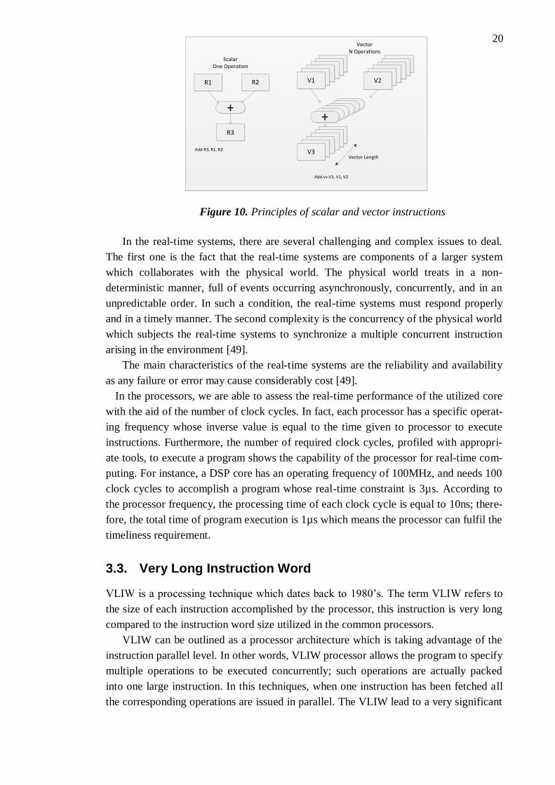
time; the Figure 10 depicts the mentioned concept simply. [43]
Wireless communication is one of the most computationally based fields which is
demanding for a huge amount of workloads, and also introduces numerous difficulties
to the design and implementation process. In this field, all the requirements must be
performed by a small mobile device and must be accomplished by a small battery which
is responsible to power the system. The main aim of the wireless communication indus-
try is to provide a seamless end-user service along high data rates, meanwhile the power
is limited. To achieve high performance and power efficient solutions, three categories
of the processors can be chosen. The first one is the application specific processors
which are very expensive and fixed-function. The second category is the usage of multi-
core processors which consist of several independent CPU lead to high power consump-
tion. The last but not least is the parallelism processors which exploiting the parallelism
concept to gain higher performance while keeping the power consumption affordable.
From the platform point of view, the parallel processors can be categorized into three
classes to compromise on both targets, namely, Very Long Instruction Word (VLIW),
vector processing and SIMD which will be discussed in the following.
3.2. Real-Time Requirement
In the recent years, the real-time processing/computing/operation has emerged as an
important discipline in the computer science and engineering. With the intensive
growth of the computational power, more systems are being implemented in the soft-
ware based solution to exploit the flexibility and sophistication afforded by the software
implementation. However, as the real-time implementations are getting more compli-
cated, the software design styles have been brought to a higher level.
Broadly speaking, real-time processing subjects the system to a real-time constraint
which means the system has to response to the input within a specific time period. The
real-time constraint is often referred to as operational deadline for each machine instruc-
tion. Thus, the ‘time’ is a source of fundamental concern in the real-time systems, and
all the instruction must be scheduled and executed to meet their timeliness require-
ments. The timeliness requirements can be classified into hard real-time where failure to
meet a deadline is treated as fatal system failure; and the soft real-time where an occa-
sional missed deadline may be tolerated.
In the field of the Digital Signal Processing (DSP), a real-time system should pro-
cess the input and output samples continuously in the time that it takes to input and out-
put the same set of samples independent of the processing delay. That means the mean
of the processing time per sample is not greater than the sampling period which is also
the reciprocal of the sampling rate.
20
In the real-time systems, there are several challenging and complex issues to deal.
The first one is the fact that the real-time systems are components of a larger system
which collaborates with the physical world. The physical world treats in a non-
deterministic manner, full of events occurring asynchronously, concurrently, and in an
unpredictable order. In such a condition, the real-time systems must respond properly
and in a timely manner. The second complexity is the concurrency of the physical world
which subjects the real-time systems to synchronize a multiple concurrent instruction
arising in the environment [49].
The main characteristics of the real-time systems are the reliability and availability
as any failure or error may cause considerably cost [49].
In the processors, we are able to assess the real-time performance of the utilized core
with the aid of the number of clock cycles. In fact, each processor has a specific operat-
ing frequency whose inverse value is equal to the time given to processor to execute
instructions. Furthermore, the number of required clock cycles, profiled with appropri-
ate tools, to execute a program shows the capability of the processor for real-time com-
puting. For instance, a DSP core has an operating frequency of 100MHz, and needs 100
clock cycles to accomplish a program whose real-time constraint is 3µs. According to
the processor frequency, the processing time of each clock cycle is equal to 10ns; there-
fore, the total time of program execution is 1µs which means the processor can fulfil the
timeliness requirement.
3.3. Very Long Instruction Word
VLIW is a processing technique which dates back to 1980’s. The term VLIW refers to
the size of each instruction accomplished by the processor, this instruction is very long
compared to the instruction word size utilized in the common processors.
VLIW can be outlined as a processor architecture which is taking advantage of the
instruction parallel level. In other words, VLIW processor allows the program to specify
multiple operations to be executed concurrently; such operations are actually packed
into one large instruction. In this techniques, when one instruction has been fetched all
the corresponding operations are issued in parallel. The VLIW lead to a very significant
R1 R2
R3
+
ScalarOne Operation R1R1R1R1R1
V1
R1R1R1R1R1V2
R1R1R1R1R1V3
++++++
Vector Length
Add R3, R1, R2
Add.vv V3, V1, V2
VectorN Operations
Figure 10. Principles of scalar and vector instructions
21
improvement which is simple hardware in a way that number of functional units can be
increased without need to any additional sophisticated hardware.
3.4. Vector Processing
Vector processing is a technique in which one instruction is executed on an entire vec-
tor. The operands to the instructions are complete vectors instead of one element. Fun-
damentally, in the vector processors, the basic idea is to read the sets of data elements
into the vector registers, and then the operation is executed on those registers. At the
end, the final results are dispersed back into the memory. In the vector processing tech-
nique, a deep level of pipelining is used to execute the element operations; meanwhile
the clock frequency can be increased. Although, deep pipeline introduces complication
from the control perspective, in the vector processing as the data elements are independ-
ent so that this problem is simply overcame.
3.4.1. Vector Processing Units
The following explained blocks are the most commonly used components in the vector
processors.
The first block is Vector Register whose length determines the maximum vector
length. These registers usually have both read and write ports. These vectors are actual-
ly specialized registers to perform the vector calculations so that they are faster and
have low startup costs. The vector register helps in significantly higher performance
compared to earlier models of the vector processors. [44]
The second one is vector functional units (FUs) which are completely pipelined and
performing new instruction in every cycle. Arithmetic and logical operations are done
within these units, moreover the load and store operation are also processed by the FUs.
The vector Load-Store Units (LSUs) are the third important blocks in the vector pro-
cessors which are responsible to move the vectors between memory and registers.
The last but not least is the Scalar registers that contain single elements or integers to
make link between LSUs, FUs and registers. In addition, they carry out the logical oper-
ations on the scalars.
It shall be noticed that one vector instruction indicates a huge amount of computa-
tion. This is as a matter of the fact that each instruction is done on the multiple data sets,
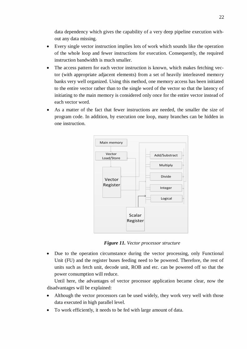
at the same time. Figure 11 depicts the main blocks in a typical vector processor.
3.4.2. Pros and Cons
In order to answer the question,” Is the usage of vector processor beneficiary or not?”,
the negative and positive aspects of them shall be reviewed. Then, regarding the appli-
cation, the significance of vector processor use will be clarified.
In the following, we first address the pros.
The computation/execution of each operation in a single vector instruction has no
22
data dependency which gives the capability of a very deep pipeline execution with-
out any data missing.
Every single vector instruction implies lots of work which sounds like the operation
of the whole loop and fewer instructions for execution. Consequently, the required
instruction bandwidth is much smaller.
The access pattern for each vector instruction is known, which makes fetching vec-
tor (with appropriate adjacent elements) from a set of heavily interleaved memory
banks very well organized. Using this method, one memory access has been initiated
to the entire vector rather than to the single word of the vector so that the latency of
initiating to the main memory is considered only once for the entire vector instead of
each vector word.
As a matter of the fact that fewer instructions are needed, the smaller the size of
program code. In addition, by execution one loop, many branches can be hidden in
one instruction.
Main memory
VectorLoad/Store
Scalar Register
Vector Register
Add/Substract
Logical
Integer
Divide
Multiply
Due to the operation circumstance during the vector processing, only Functional
Unit (FU) and the register buses feeding need to be powered. Therefore, the rest of
units such as fetch unit, decode unit, ROB and etc. can be powered off so that the
power consumption will reduce.
Until here, the advantages of vector processor application became clear, now the
disadvantages will be explained:
Although the vector processors can be used widely, they work very well with those
data executed in high parallel level.
To work efficiently, it needs to be fed with large amount of data.
Figure 11. Vector processor structure

23
On the scalar data processing, there is a deep lack of good performance which
makes the vector processors inefficient compared to the normal processors.
The cost of vector processors compared to the other processors is relatively high,
which is resulting from the need of specific design for each application, high speed
on-chip memories, difficulty in packaging and keeping the innovative architectural
design to achieve lower cost.
Due to the vectorized execution, there is high level of complexity in the codes. It has
been also found that sometimes the code alignment shall be done manually to
achieve better performance.
Besides all the aforementioned parameters, generally the performance of the vector
processors is still dependent on the length of operand vector, data dependencies and
structural hazards which will even introduce more difficulties.
All these positive and negative aspects altogether contribute in specific features to
the vector processors and indicate that vector processors need necessary modifications
to become widely popular. [43]
3.4.3. Main Operations
Although the vector processors are operating similar to the normal processors, due to
their specific features and architecture, the main operational mechanism is worth study-
ing.
A typical vector processor is capable to add two vectors to produce a third vector. It
can also subtract two vectors to generate a third one. Multiplication and division of two
vectors to make a third vector is applicable in the vector processors.
By having special Load and Store units, it is possible to read and write vectors from
or to the memory similar to the normal processors, but in the vector processors these
kinds of processes can be executed faster.
Under the certain circumstances depending on the processor, the following instruc-
tions can be also done. Inner product (multiplication and accumulation) and outer prod-
uct of two vectors are feasible to be done, but the important point is that these opera-
tions produce an array from vectors whose elements can be used as primitive data, yet.
Product between arrays can be done only for small arrays.
3.4.4. Optimization Schemes
From the optimization point of view, different techniques have been used and applied
into the vector processors to achieve the most efficient performance in terms of power,
code size and speed.
First of all, the usage of banked-memory reduces the latency for load/store instruc-
tion. In fact, the continuous or regular memory access patterns are defined in the
wide/banked-memory to accelerate the load and store instructions.
As mentioned earlier, the length of vector processor is limited. In the practical im-
plementation, the data lengths are usually greater than the Maximum Vector Length
24
(MVL) so that strip mining solution is proposed. Assume that the data length is
, to process this data vector in a parallel manner, first a loop is made to han-
dle the MLV elements. Then, another loop is generated to process the ele-
ments.
Vectorized operation within the conditional statement (if) cannot be done; therefore
Vector Mask Registers (VMRs) are used to store the test results for the next use. Gener-
ally, the Vector processors have multiple pipelines of different types. Sometimes, the
output of one pipeline instruction can be directly released into another pipeline. This
technique is called chaining, to eliminate the intermediate storage between tow pipe-
lines. [45] For instance, in the following example, it can be seen that the output vector
V1 is released to the next instruction:
MULV.D V1, V2, V3
ADDV.D V4, V1, V5
In some of the vector processors, special scatter, gather and masking instructions are
used to process the sparse matrices efficiently. All these optimization makes the vector
processors extremely faster and more efficient. [46]
3.4.5. Power Consumption
In order to evaluate the power consumption of the vector processors, there are some
parameters which effect the power consumption. The first point is that there is trade-off
between parallelism and power, the more parallelization, the less power is consumed.
The simpler instruction and logic for execution large number of operation leads to lower
power usage. In this way, there should not be multiple issues or dynamic operation logic
as the process would become complicated and the power consumption increases. It has
also been found that conditional execution results in further power saving.
By taking into account all the above mentioned methods, namely, optimization
schemes and power consumption tips, we can optimize the vector processor perfor-
mance as much as possible, which leads to lower power consumption and much more
efficient performance while fulfilling the requirements.
3.5. Single Instruction Multiple Data
SIMD is a parallelism architecture which exploits data parallelism as opposed to the
VLIW where the parallelism is used in the instructions. This technique has been added
to the general purpose DSP and multimedia processors to afford a power efficient meth-
od of parallel processing.
The SIMD can be described as an architectural feature which includes a set of in-
structions that can speed up an application performance by allowing basic operation to
be performed on multiple data elements in parallel with fewer instructions. By this
means, the main difference between SIMD and vector processing is in the way that data
elements are fed; in SIMD a stream of data elements are processed. However, it can be
25
said that vector processing machines apply the operation on the vector one element at a
time through the pipeline processors, while the SIMD machines process all the element
of the stream, simultaneously. In other words, the vector processors are SIMD opera-
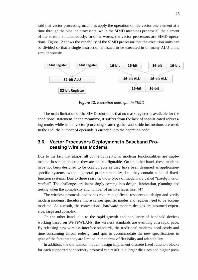
tions. Figure 12 shows the capability of the SIMD processor that the execution units can
be divided so that a single instruction is issued to be executed in on many ALU units,
simultaneously.
32-bit Register 32-bit Register
32-bit ALU
32-bit Register
16-bit 16-bit 16-bit 16-bit
16-bit ALU 16-bit ALU
16-bit 16-bit
Figure 12. Execution units split in SIMD
The main limitation of the SIMD solution is that no mask register is available for the
conditional statement. In the meantime, it suffers from the lack of sophisticated address-
ing mode, while in the vector processing scatter-gather and stride instructions are used.
In the end, the number of operands is encoded into the operation code.
3.6. Vector Processors Deployment in Baseband Pro-cessing Wireless Modems
Due to the fact that almost all of the conventional modems functionalities are imple-
mented in semiconductor, they are not configurable. On the other hand, these modems
have not been designed to be configurable as they have been designed as application-
specific systems, without general programmability, i.e., they contain a lot of fixed-
function systems. Due to these reasons, those types of modem are called “fixed-function
modem”. The challenges are increasingly coming into design, fabrication, planning and
testing when the complexity and number of air interfaces rise. [47]
The wireless protocols and bands require significant resources to design and verify
modern modems; therefore, more carrier specific modes and regions need to be accom-
modated. As a result, the conventional hardware modem designs are assumed expen-
sive, large and complex.
On the other hand, due to the rapid growth and popularity of handheld devices
working based on Wi-Fi/WLANs, the wireless standards are evolving at a rapid pace.
By releasing new wireless interface standards, the traditional modems need costly and
time consuming silicon redesign and spin to accommodate the new specifications in
spite of the fact that they are limited in the terms of flexibility and adaptability.
In addition, the old fashion modem design implement discrete fixed function blocks
for each supported connectivity protocol can result in a larger die sizes and higher pow-
26
er consumption. Consequently, the conventional fixed function modems, with their
lengthy design cycles, requirement for discrete fixed function hardware and lack of
adaptability requires the chips that are larger, inefficient, expensive and complex.
The limited compatibility of the fixed function modems leads to less competitive
products. The users experience less optimal performance, expensive devices and fewer
choices. Meanwhile, the network providers have to yield lower device performance and
increased network capital expenditure costs.
The new wireless communication standards include new specifications, which result
in more complexity in System-on-Chip (SoC) implementation. Therefore, relying on the
sequential processors is not practical anymore. One technique to improve the flexibility,
compatibility and adaptability of the baseband modems is the usage of processors with a
specific application to replace the fixed function units. For example, utilizing the vector
processors or SIMD processors is beneficial in term of cost. The applicability of the
SIMD processors is feasible due to the fact that in the baseband processing modem,
some of the data processing can be done in parallel. In fact, the baseband signal pro-
cessing in the wireless modem contains such data parallelism, in principle. [48]
3.7. ConnX BBE32 DSP Core
As mentioned earlier, the incompatibility features of the ASIC baseband processing
platforms with the evolving standards, fast time-to-market and long platform lives has
brought the significance of the configurable DSP core to a higher level.
One particular VLIW machine is ConnX BBE32 which is a specific application pro-
cessor for the next generation of baseband processors like LTE advanced, 4G cellular
networks and multi-standards broadcast transceivers will be studied. Primarily, for such
applications, high efficient computational cores are required to have high degree of par-
allelism in architecture. The ConnX BBE32 is built around the baseline Xtensa RISC
architecture which implements a rich set of generic instructions optimized for efficient
embedded processing. The power of the ConnX BBE32 comes from a comprehen-
sive set of over 350 DSP and baseband optimized instructions excluding the
baseline Xtensa RISC instructions. Hence, it can be summarized that he ConnX
BBE32 is built on Tensilica’s proven Xtensa LX customizable processor architecture,
and is specifically designed to support the needs of software-based baseband processing.
The BBE32 DSP is 4-way VLIW processor, which contains vector processing and
SIMD-extensions. This DSP engine fulfills the mentioned requirements by combining a
16-way Single Instruction Multiple Data (SIMD), 32 Multiplier-ACcumulators (MAC),
4-slot VLIW processing pipeline with a rich and extensible interfaces. It constitutes two
groups of memories, Instruction (I-RAM) and Data (D-RAM0, D-RAM1) memories,
for higher efficiency. [50]
BBE32 contains a comprehensive toolset of softwares such as high performance
C/C++ compiler with automatic vectorization to support the VLIW pipeline. This pro-
cessor is capable to execute four operations in parallel in every cycle; such massive op-
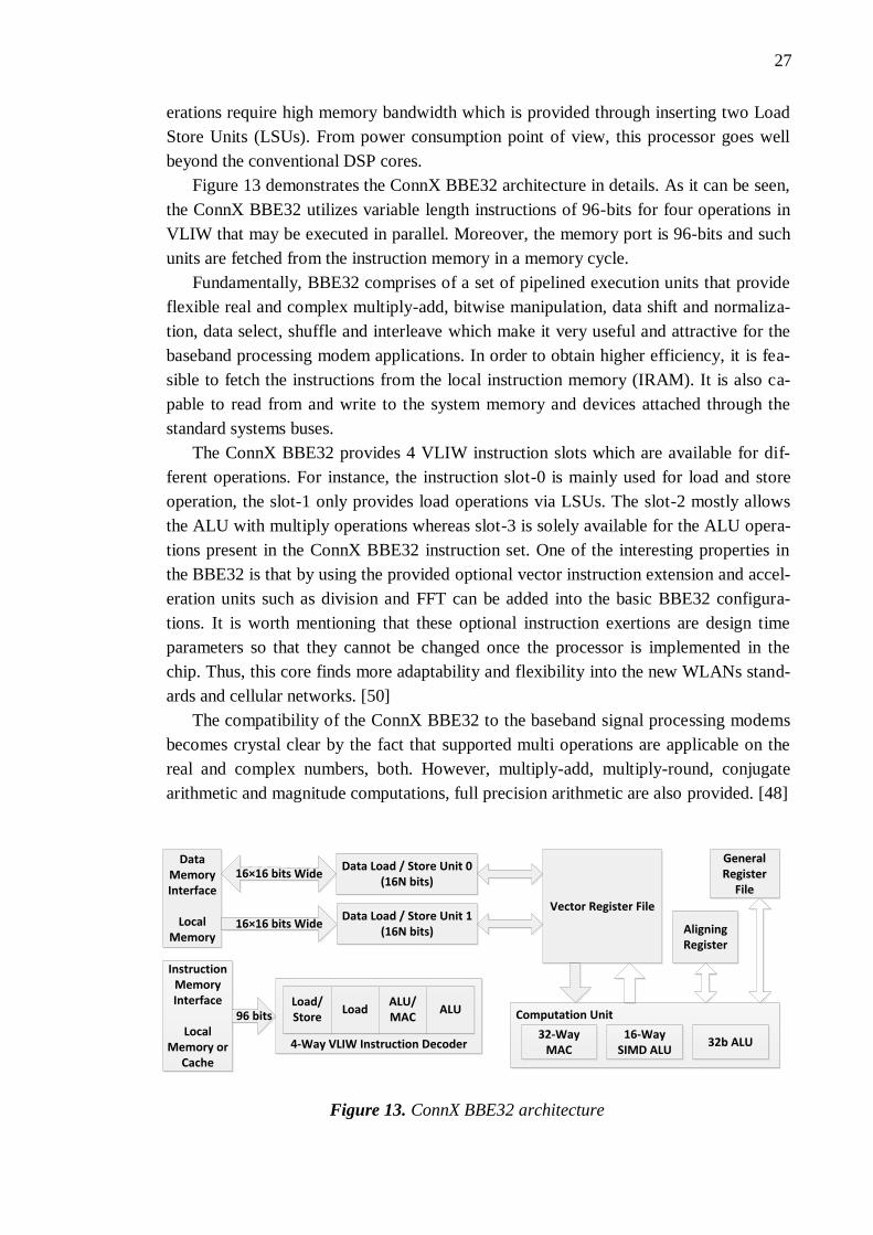
27
erations require high memory bandwidth which is provided through inserting two Load
Store Units (LSUs). From power consumption point of view, this processor goes well
beyond the conventional DSP cores.
Figure 13 demonstrates the ConnX BBE32 architecture in details. As it can be seen,
the ConnX BBE32 utilizes variable length instructions of 96-bits for four operations in
VLIW that may be executed in parallel. Moreover, the memory port is 96-bits and such
units are fetched from the instruction memory in a memory cycle.
Fundamentally, BBE32 comprises of a set of pipelined execution units that provide
flexible real and complex multiply-add, bitwise manipulation, data shift and normaliza-
tion, data select, shuffle and interleave which make it very useful and attractive for the
baseband processing modem applications. In order to obtain higher efficiency, it is fea-
sible to fetch the instructions from the local instruction memory (IRAM). It is also ca-
pable to read from and write to the system memory and devices attached through the
standard systems buses.
The ConnX BBE32 provides 4 VLIW instruction slots which are available for dif-
ferent operations. For instance, the instruction slot-0 is mainly used for load and store
operation, the slot-1 only provides load operations via LSUs. The slot-2 mostly allows
the ALU with multiply operations whereas slot-3 is solely available for the ALU opera-
tions present in the ConnX BBE32 instruction set. One of the interesting properties in
the BBE32 is that by using the provided optional vector instruction extension and accel-
eration units such as division and FFT can be added into the basic BBE32 configura-
tions. It is worth mentioning that these optional instruction exertions are design time
parameters so that they cannot be changed once the processor is implemented in the
chip. Thus, this core finds more adaptability and flexibility into the new WLANs stand-
ards and cellular networks. [50]
The compatibility of the ConnX BBE32 to the baseband signal processing modems
becomes crystal clear by the fact that supported multi operations are applicable on the
real and complex numbers, both. However, multiply-add, multiply-round, conjugate
arithmetic and magnitude computations, full precision arithmetic are also provided. [48]
Figure 13. ConnX BBE32 architecture
Data Memory Interface
Local Memory
Instruction Memory Interface
Local Memory or
Cache
16×16 bits Wide
16×16 bits Wide
96 bits
Data Load / Store Unit 0(16N bits)
Data Load / Store Unit 1(16N bits)
Load/Store
LoadALU/MAC
ALU
Vector Register File
Aligning Register
General Register
File
General Register
File
4-Way VLIW Instruction Decoder32-Way
MAC16-Way
SIMD ALU32b ALU
Computation Unit
28
Due to the specific applications that the processor is designed for, ten optional pack-
ages are considered to be supported which lead to the processing acceleration, as fol-
lowing:
Aligning Load and Store package,
8-way integer and fractional vector divide package
16-way vector reciprocal square root package
Bit-multiplication support for LFSR application and convolutional encoding
3-GPP soft-bit demapping package
FIR package
Symmetric FIR package
Pairwise real multiply package
FFT package
Linear block decoder package
By the provided packages, especially FFT and FIR ones, the baseband signal pro-
cessing would be easier.
It is worth mentioning that Tensilica has provided two different processor configura-
tions, namely Low-Power (LP) and Performance-Maximized (PM) which are used in
this research. Basically, the LP version of the ConnX BBE32 has only the base ConnX
BBE32 instruction sets. The PM configuration includes all ten optional packag-
es/accelerators instructions which are available in Xtensa Xplorer for ConnX BBE32
[50].
In addition to the optional packages, the ConnX BBE32 has a categorized set of the
register files to deliver larger bandwidth and lower memory traffic. The first one com-
prises of sixteen 256-bit general purpose narrow vector registers (vec) capable of keep-
ing operands and SIMD operations results. The second set consists of four 640-bit wide
vector registers (wvec). Principally, the interface between the data memories the wide
vector registers takes place through the narrow registers. In addition to the mentioned
vector registers, other kind of optional registers are provided in the BBE32, which are
helpful in flexibility and VLIW application, namely, Boolean vectors, Alignment regis-
ters and variable Shift/Select registers. [50, 51]

29
4. IEEE802.11AC TRANSMITTER IMPLEMENTA-
TION
Through this chapter, the detailed data structure defined by the IEEE standard will be
reviewed. In addition, the desired transmission scenario’s requirements including the
antenna configuration, modulation scheme, coding rate and bandwidth will be defined.
Moreover, the implementation procedure for each transmission mode will be described,
as well. It shall be mentioned that in the following chapter, the draft version of
IEEE802.11ac standard has been followed in this research [52].
4.1. Data Structure
In this project, the transmitter is designed in such a way to support the desired operating
points. As mentioned earlier, our main focus is on the PHY layer implementation of the
IEEE802.11ac standard rather than the MAC specifications.
According to the standard definition, the VHT packet structure is composed of three
parts. The first part is the legacy preamble, the second one is the VHT preamble, and the
last one is the data part. Figure 14 illustrates the VHT packet structure. The legacy por-
tion consists of the several fields, namely, L-STF, L-LTF and L-SIG, which are de-
scribed in the following. The VHT part also includes the VHT-SIG-A, VHT-SIG-B,
VHT-STF and VHT-LTF fields. Table 2 defines each field. [52]
As the frequency domain processing of the VHT-SIG-B field of the preamble part
and the data field is performed on the DSP, the study is mainly carried out for these two
fields.
Figure 14. VHT packet structure
L-STF L-LTF L-SIG VHT-SIG-AVHT-STF
VHT-LTFVHT-SIG-B
Data
8 µs 8 µs4 µs per VHT-LTF
symbol8 µs4 µs 4 µs 4 µs
Legacy Preamble VHT Preamble VHT Data
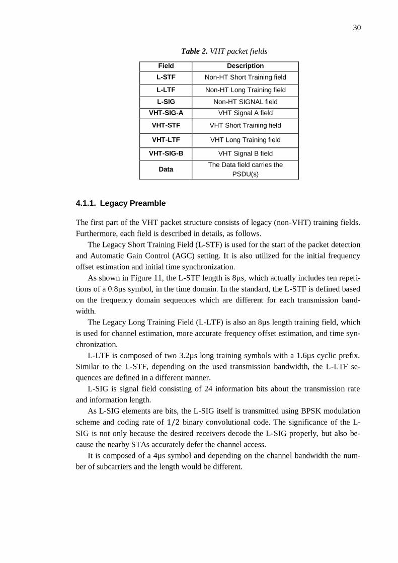
30
Table 2. VHT packet fields
4.1.1. Legacy Preamble
The first part of the VHT packet structure consists of legacy (non-VHT) training fields.
Furthermore, each field is described in details, as follows.
The Legacy Short Training Field (L-STF) is used for the start of the packet detection
and Automatic Gain Control (AGC) setting. It is also utilized for the initial frequency
offset estimation and initial time synchronization.
As shown in Figure 11, the L-STF length is 8µs, which actually includes ten repeti-
tions of a 0.8µs symbol, in the time domain. In the standard, the L-STF is defined based
on the frequency domain sequences which are different for each transmission band-
width.
The Legacy Long Training Field (L-LTF) is also an 8µs length training field, which
is used for channel estimation, more accurate frequency offset estimation, and time syn-
chronization.
L-LTF is composed of two 3.2µs long training symbols with a 1.6µs cyclic prefix.
Similar to the L-STF, depending on the used transmission bandwidth, the L-LTF se-
quences are defined in a different manner.
L-SIG is signal field consisting of 24 information bits about the transmission rate
and information length.
As L-SIG elements are bits, the L-SIG itself is transmitted using BPSK modulation
scheme and coding rate of binary convolutional code. The significance of the L-
SIG is not only because the desired receivers decode the L-SIG properly, but also be-
cause the nearby STAs accurately defer the channel access.
It is composed of a 4µs symbol and depending on the channel bandwidth the num-
ber of subcarriers and the length would be different.
Field Description
L-STF Non-HT Short Training field
L-LTF Non-HT Long Training field
L-SIG Non-HT SIGNAL field
VHT-SIG-A VHT Signal A field
VHT-STF VHT Short Training field
VHT-LTF VHT Long Training field
VHT-SIG-B VHT Signal B field
Data The Data field carries the
PSDU(s)
31
4.1.2. Very High Throughput Preamble
VHT preamble of the VHT packet structure begins with VHT-SIG-A and continues
with VHT-STF, VHT-LTF and VHT-SIG-B.
VHT-SIG-A field carries the required information to interpret VHT PPDUs. VHT-
SIG-A field consists of two parts, namely VHT-SIG-A1 and VHT-SIG-A2; each of
which consists of 24 bits. VHT-SIG-A1 is transmitted before VHT-SIG-A2.
VHT-SIG-A totally contains 48 bits carrying the information related to the band-
width, number of space time streams, transmit beam forming, modulation and coding
scheme, and the guard interval type (short/long).
The signaling part of VHT waveform will be started by the VHT Short Training
Field (VHT-STF). By receiving this field, we switch onto the cyclic shift diversity table
which is specifically defined for VHT preamble fields.
The main purpose of the VHT-STF field is to improve the automatic gain control es-
timation in a MIMO transmission. The duration of the VHT-STF field is 4μs. The fre-
quency domain sequence is used to construct the VHT-STF field in a 20 MHz transmis-
sion which is identical to the L-STF field. In a 40 MHz and an 80 MHz transmission,
the VHT-STF field is constructed from the 20 MHz version by frequency shifting a du-
plicate of it to each 20 MHz subchannel and applying appropriate phase rotations per 20
MHz subchannel.
VHT Long Training Field (VHT-LTF) is conceptually similar to the HT-LTF with
some new sequences for wider channel bandwidths 80MHz and 160MHz. By this
means, the construction procedure has these two main differences: the first one is the
presence of up to 8 spatial streams, and the second is allowance for phase tracking dur-
ing VHT-LTF. It is a 4µs frame per VHT-LF symbol.
The VHT-LTF provides a means for the receiver to estimate the MIMO channel be-
tween the set of constellation mapper outputs (or, if STBC is applied, the STBC encoder
outputs) and the receive chains. It should be noted that the channel estimation is done by
using the pilot subcarriers inserted into the VHT-LTF symbols.
Although the primary purpose of using VHT-SIG-B is for signaling user specific in-
formation in a MU packet, it is still used in all packets to maintain an unified preamble
format for VHT packets. However, in SU scenario, the receiver does not need to process
VHT-SIG-B. Since VHT-SIG-B is coming after VHT-STF and VHT-LTF, it is formed
differently than VHT-SIG-A in such a way that in our system the bits are repeated in-
cluding the tail bits. By this means, the processing gain at the receiver is obtained by
averaging repeated soft values at the decoder input.
As shown in Figure 14, VHT-SIG-B is a 4µsec OFDM symbol with single stream,
BPSK, BCC rate 1/2 modulation. In our systems, the channel bandwidth is 80MHz
which means there are 29 bits available in VHT-SIG-B consisting of 23 information bits
and 6 tail bits, each repeated four times, with a single pad bit appended at the end.
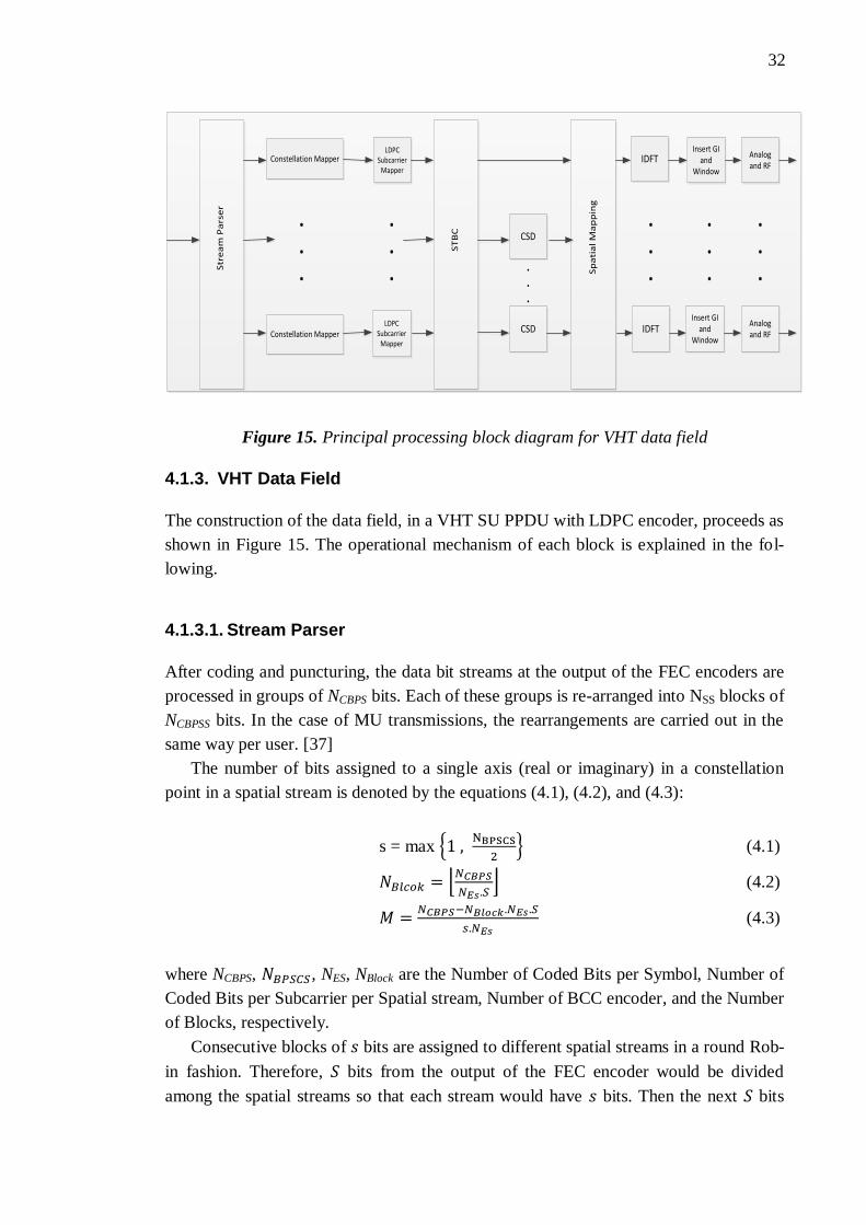
32
Figure 15. Principal processing block diagram for VHT data field
4.1.3. VHT Data Field
The construction of the data field, in a VHT SU PPDU with LDPC encoder, proceeds as
shown in Figure 15. The operational mechanism of each block is explained in the fol-
lowing.
4.1.3.1. Stream Parser
After coding and puncturing, the data bit streams at the output of the FEC encoders are
processed in groups of NCBPS bits. Each of these groups is re-arranged into NSS blocks of
NCBPSS bits. In the case of MU transmissions, the rearrangements are carried out in the
same way per user. [37]
The number of bits assigned to a single axis (real or imaginary) in a constellation
point in a spatial stream is denoted by the equations (4.1), (4.2), and (4.3):
s = max {
} (4.1)
⌊
⌋ (4.2)
(4.3)
where NCBPS, , NES, NBlock are the Number of Coded Bits per Symbol, Number of
Coded Bits per Subcarrier per Spatial stream, Number of BCC encoder, and the Number
of Blocks, respectively.
Consecutive blocks of bits are assigned to different spatial streams in a round Rob-
in fashion. Therefore, bits from the output of the FEC encoder would be divided
among the spatial streams so that each stream would have bits. Then the next bits
Str
ea
m P
ars
er
ST
BC
Sp
ati
al
Ma
pp
ing
Constellation Mapper
Constellation Mapper
LDPC Subcarrier
Mapper
LDPC Subcarrier
Mapper
CSD
CSD
Analog and RF
Insert GI and
Window
IDFT
IDFTInsert GI
and Window
Analog and RF
.
.
.
.
.
.
.
.
.
.
.
.
.
.
....
33
from the output of the encoder are used, at some point if the number of the is
greater than , then the last bits of each OFDM
symbol are provided by taking bits from the output of the first encoder. By this
means, each stream (streams 1 to M) would take s bits, in continuation bits from
the output of the next encoder are used to feed the spatial stream .
4.1.3.2. Constellation Mapper
The OFDM subcarriers shall be modulated by using BPSK, QPSK, 16-QAM, 64-QAM,
or 256-QAM, depending on the data rate requested. The encoded and interleaved binary
serial input data shall be divided into groups of NBPSC (1, 2, 4, 6, or 8) bits and converted
into complex numbers representing BPSK, QPSK, 16-QAM, 64-QAM, or 256QAM
constellation points, respectively. The conversion shall be performed according to Gray-
coded constellation mappings with the input bit b0 being the earliest in the stream. The
output values d are formed by multiplying the resulting ( ) value by a normaliza-
tion factor KMOD (which depends on the base modulation mode), defined as follows:
( ) (4.4)
It should be noted that modulation type can differ from the start to the end of the
transmission, as the signal changes from SIGNAL to DATA. However, in case of using
256-QAM modulation, a normalization/scaling factor should be used which is
√ .
4.1.3.3. Low-Density Parity Check Tone Mapper
The LDPC tone mapping shall be performed on all LDPC encoded streams as described
in the chapter 2 by using an LDPC tone-mapping distance parameter DTM. DTM is con-
stant for each bandwidth and its values for different bandwidths are shown in Table 3.
LDPC tone mapping shall not be performed on streams that are encoded using BCC.
Table 3. LDPC tone mapping distance for different bandwidth
Parameter 20MHz 40MHz 80MHz 160 MHz,
80+80 MHz
4 6 9 9
The objective of the LDPC tone mapper is to map consecutive OFDM symbols to
non-consecutive subcarriers. It is worth noticing that LDPC tone mapping is done per
OFDM symbol.
LDPC tone mapping is done by altering the incoming streams of complex numbers
from the constellation mapper; meaning, it shuffles the data subcarriers in each OFDM
symbol in each stream of complex numbers. The equation (4.5) presents how LDPC
tone mapper works:
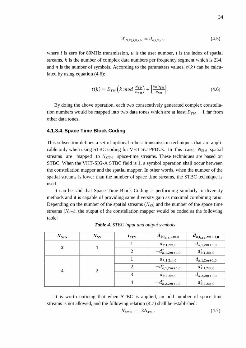
34
( ) (4.5)
where is zero for 80MHz transmission, is the user number, is the index of spatial
streams, is the number of complex data numbers per frequency segment which is 234,
and is the number of symbols. According to the parameters values, ( ) can be calcu-
lated by using equation (4.6):
( ) (
) ⌊
⌋ (4.6)
By doing the above operation, each two consecutively generated complex constella-
tion numbers would be mapped into two data tones which are at least far from
other data tones.
4.1.3.4. Space Time Block Coding
This subsection defines a set of optional robust transmission techniques that are appli-
cable only when using STBC coding for VHT SU PPDUs. In this case, NSS,0 spatial
streams are mapped to NSTS,0 space-time streams. These techniques are based on
STBC. When the VHT-SIG-A STBC field is 1, a symbol operation shall occur between
the constellation mapper and the spatial mapper. In other words, when the number of the
spatial streams is lower than the number of space time streams, the STBC technique is
used.
It can be said that Space Time Block Coding is performing similarly to diversity
methods and it is capable of providing same diversity gain as maximal combining ratio.
Depending on the number of the spatial streams (NSS) and the number of the space time
streams (NSTS), the output of the constellation mapper would be coded as the following
table:
Table 4. STBC input and output symbols
2 1 1
2
4 2
1
2
3
4
It is worth noticing that when STBC is applied, an odd number of space time
streams is not allowed, and the following relation (4.7) shall be established:
. (4.7)

35
4.1.3.5. Pilot Insertion
According to the channelization presented in the chapter 2, for a 20 MHz transmis-
sion, four pilot tones shall be inserted in subcarriers { } For a 40 MHz
transmission, six pilot tones shall be inserted in subcarriers –53, –25, –11, 11, 25, and
53.
For an 80 MHz transmission mode, eight pilot tones shall be inserted in subcarriers
{– – – – }. The pilot mapping of subcarrier of sym-
bol shall be specified based on the following equations:
{ } { ( ) ( ) } (4.8)
{ } (4.9)
where is defined according to table 5:
Table 5. Pilot values for 80MHz transmission bandwidth
1 1 1 -1 -1 1 1 1
In addition to these pilot subcarriers, 14 null subcarriers shall be inserted into the da-
ta streams resulting in data streams containing 256 subcarriers.
4.1.3.6. Cyclic Shift Diversity
Cyclic shift diversity is applied to each OFDM symbol separately in order to decorrelate
the transmitted signals from different antennas and prevent from bad beam forming ef-
fects. Based on the number of the space time streams, would be applied to the
OFDM symbols according to the equation (4.10):
( ) ( ) . (4.10)
Table 6. Cyclic shift values for data field packets
Spatial stream 1 2 3 4
1 0 ns ----- ----- -----
2 0 ns -400 ns ----- -----
3 0 ns -400 ns -200 ns -----
4 0 ns -400 ns -200 ns -600 ns
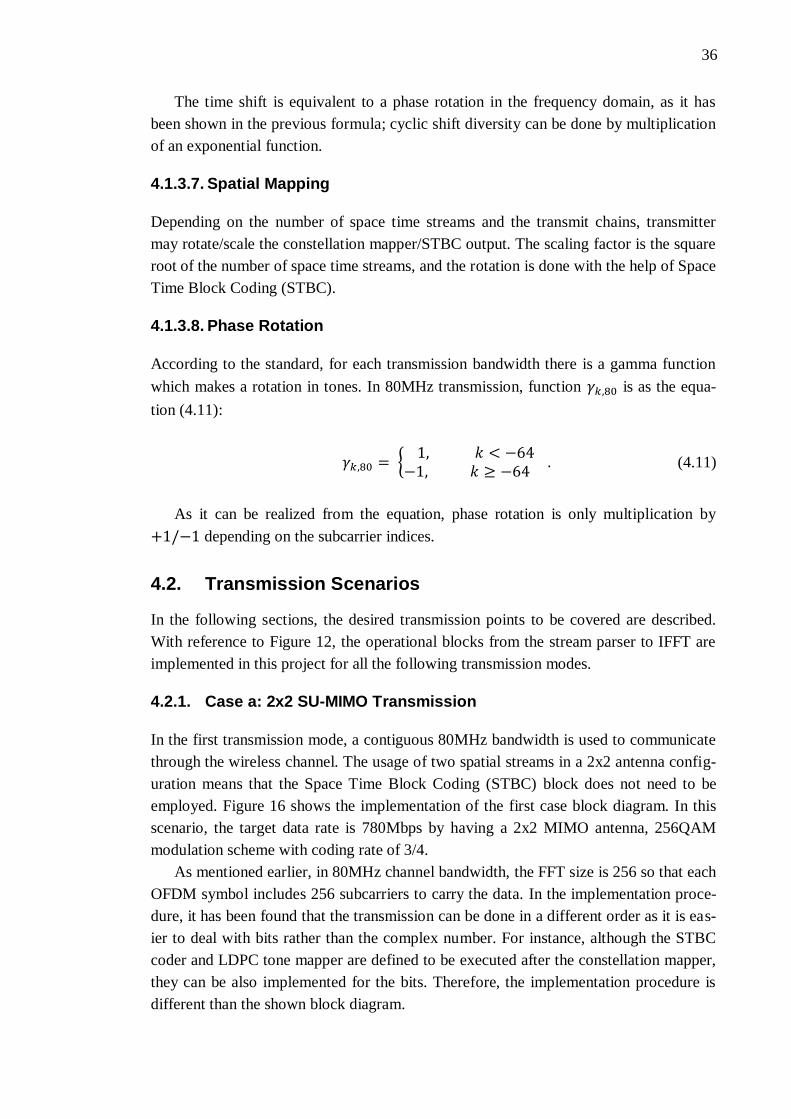
36
The time shift is equivalent to a phase rotation in the frequency domain, as it has
been shown in the previous formula; cyclic shift diversity can be done by multiplication
of an exponential function.
4.1.3.7. Spatial Mapping
Depending on the number of space time streams and the transmit chains, transmitter
may rotate/scale the constellation mapper/STBC output. The scaling factor is the square
root of the number of space time streams, and the rotation is done with the help of Space
Time Block Coding (STBC).
4.1.3.8. Phase Rotation
According to the standard, for each transmission bandwidth there is a gamma function
which makes a rotation in tones. In 80MHz transmission, function is as the equa-
tion (4.11):
{
(4.11)
As it can be realized from the equation, phase rotation is only multiplication by
depending on the subcarrier indices.
4.2. Transmission Scenarios
In the following sections, the desired transmission points to be covered are described.
With reference to Figure 12, the operational blocks from the stream parser to IFFT are
implemented in this project for all the following transmission modes.
4.2.1. Case a: 2x2 SU-MIMO Transmission
In the first transmission mode, a contiguous 80MHz bandwidth is used to communicate
through the wireless channel. The usage of two spatial streams in a 2x2 antenna config-
uration means that the Space Time Block Coding (STBC) block does not need to be
employed. Figure 16 shows the implementation of the first case block diagram. In this
scenario, the target data rate is 780Mbps by having a 2x2 MIMO antenna, 256QAM
modulation scheme with coding rate of 3/4.
As mentioned earlier, in 80MHz channel bandwidth, the FFT size is 256 so that each
OFDM symbol includes 256 subcarriers to carry the data. In the implementation proce-
dure, it has been found that the transmission can be done in a different order as it is eas-
ier to deal with bits rather than the complex number. For instance, although the STBC
coder and LDPC tone mapper are defined to be executed after the constellation mapper,
they can be also implemented for the bits. Therefore, the implementation procedure is
different than the shown block diagram.
37
Figure 16. Principal block diagram of Case a
At the beginning, an additional block called preparation block is used to rearrange
the incoming bit streams to become ready for LDPC tone mapping and modulation. As
for the processor is 16-bits, the preparation block rearranges the data in the frames of
16-bits. The incoming bit stream has , and has the following format. From
left to right, the first and second 4 bits actually present the real part of the first and sec-
ond streams (first subcarrier), respectively. In the meantime, the third and fourth 4 bits
show the first and second streams imaginary parts (first subcarrier), correspondingly.
Therefore, the preparation block combines the real and imaginary parts of each subcar-
rier in such a way that the first outcoming 16-bits frame has the real parts of two
streams, and the second 16-bits frame has the imaginary parts (8 bits in both frames are
zero). Then, two streams of complex numbers are ready to be fed into the LDPC tone
mapper.
In the LDPC tone mapper, the data subcarriers of both streams are shuffled at the
same time. According to the provided information in section 4.1.3.3., LDPC tone map-
per alters the subcarriers’ location of each OFDM symbol in each stream. It is worth of
noticing that the incoming data streams are aligned to 32 bytes which means streams of
complex numbers with bits are processed, although the original number of data
subcarriers is 234.
It has been found that if the stream parser and constellation mapper are combined,
the performance would be most optimized. Therefore in the third phase, the LDPC tone
mapped streams of complex numbers are parsed and mapped into the constellation
mapper, simultaneously. As explained earlier, streams parser parses coded
bits per symbol (NCBPS) between two streams that means each stream would have
coded bits per symbol, meaning, each stream has 8 bits including 4 bits for real
part and 4 bits for the imaginary part. By using 256-QAM modulation, every 8 bits are
simultaneously mapped into one 256-QAM constellation point.
According to the specifications given in section 4.1.3, all the functions after the
LDPC tone mapper including pilot insertion, Cyclic Shift Diversity (CSD), spatial map-
Stream parser
256QAM
DATA field – case aFrom stream parser to IFFT
Output bits from the
LDPC encoder
256QAM
LDPC tone mapper
LDPC tone mapper
Pilot Insertion
CSD
AntennaMapping
Stream 1
Stream 2
y0 y1y2 … y3744 = 234*8*2
y0, y1, y2, y3, y8, y9, y10, y11, …
y4, y5, y6, y7, y12, y13, y14, y15, …
Phase Rotation

38
ping and phase rotation are originally based on multiplication between the data subcar-
riers and coefficients. Due to this reason, they can be merged into one block and execut-
ed in one operation. Consequently, the outcoming streams from the stream parser and
constellation mapper block will be processed in one block to be ready for the IFFT op-
eration. For this purpose, we created a look up table including all those numerical values
resulted from the mentioned operations to be multiplied by the data subcarriers. There
are several remarkable points, the first one is that due to the existence of two space time
streams, the spatial mapping is only a scaling operation with the scaling factor of
√ .
The second one is originated from the repetitive nature of the cyclic shift diversity val-
ues for the data subcarriers meaning the CSD table is duplicated for every eight subcar-
riers. The last point but not the least is that the first stream remained unchanged while
the second one is shifted by 400ns in the time domain under the CSD operation.
4.2.2. Case b: 4x4 SU-MIMO Transmission
Similar to the previous case, the usage of 80MHz bandwidth provides 256 subcarriers to
send the data. In addition, transmission of four spatial streams through a 4x4 antenna
configuration results in the data rate of 1560Mbps by having modulation scheme
256QAM with coding rate of 3/4. It is worth mentioning that the equal number of spa-
tial streams and the space time streams, STBC is not employed. The transmission block
diagram for this case is shown in Figure 17.
Due to the fact that the processor is 16-bits, the incoming bits streams shall be rear-
ranged. But in this case, as 4 spatial streams are used, the first incoming 16 bits already
feature the real part of the first subcarrier of each stream, and the second 16 bits are the
imaginary parts. By this means, the desired 16-bits packets are ready so that no prepara-
tion is needed and the bit streams can be directly fed into the LDPC tone mapper.
According to the standard, the LDPC tone mapper maps the OFDM symbols into the
other indices by a sufficient distance to avoid any distortion.
After shuffling the data bits in the LDPC tone mapping block, the stream parser al-
locates 8 bits to each stream and maps them into one constellation point, at the same
time. Therefore, stream parser parses coded bits per symbol (NCBPS) among
four streams that results in each stream having coded bits per symbol, mean-
ing, each stream has 8 bits including 4 bits for real part and 4 bits for the imaginary part.
By using 256-QAM modulation, every 8 bits are simultaneously mapped into one 256-
QAM constellation point.
The rest of operation, namely pilot insertion, cyclic shift diversity, spatial mapping
and phase rotation, similar to the previous case, are done by multiplication between the
look up table numerical values and data subcarriers. The scaling factor for the spatial
mapping operation would be
√ , and the cyclic shift diversity in this scenario would
make change in all the spatial streams except the first one. As a result, the first stream
would be remained unchanged, but the second, third and fourth streams are shifted in

39
Figure 17. Principal block diagram of Case b
the time domain by 400ns, 200ns and 600ns respectively. The phase rotation is also a
multiplication with depending on the subcarrier index.
4.2.3. Case c: 2x2 Antenna Configuration with 1x1 SU-SISO Transmission
In this case, the application of 80MHz bandwidth, 256-QAM modulation scheme and
2x2 antenna configuration leads to 390Mbps data rate. The additional antenna is as-
sumed to be used at both sides to achieve diversity gain. Here, the number of spatial
streams is lower than the space time streams number which brings up the idea of em-
ploying STBC encoder. Figure 18 shows the transmission structure for the third trans-
mission scenario.
Due to the unequal number of the spatial streams and space time streams, the STBC
encoding method must be employed. We apply STBC in this step as it is easier to pro-
cess the bits rather than the complex numbers. According to the STBC description (giv-
en in Table 22-20 in the standard specification), some symbols need to be conjugated
i.e. the imaginary part should be negated and in bit level this only means inverting the
sign bit for the imaginary part. For that reason, it is possible to do the STBC coding in
the preparation block, as well. Consequently, in this block, the incoming stream of size
bits is duplicated and for some of them (depending on the index) the sign bit is
changed. At the end, two streams of the size of bits come out to be fed into the
LDPC tone mapper.
After applying the STBC coding into the streams, LDPC tone mapper is applied in
which the bit streams are interleaved or replaced into new data tones. By this means, the
output is LDPC tone mapped STBC coded bit streams.
Stream parser
256QAM
DATA field – case bFrom stream parser to IFFT
Output bits from the LDPC encoder
256QAM
LDPC tone mapper
LDPC tone mapper
Pilot Insertion
CSD
AntennaMapping
Stream 1
Stream 2
y0 y1y2 … y7488 = 234*8*4
y0, y1, y2, y3, y16, y17, y18, y19, …
y4, y5, y6, y7, y20, y21, y22, y23, …
Phase Rotation
256QAM
256QAM
LDPC tone mapper
LDPC tone mapper
CSD
Stream 3
Stream 4
y8, y9, y10, y11, y24, y25, y26, y27, …
y12, y13, y14, y15, y28, y29, y30, y31, …
CSD
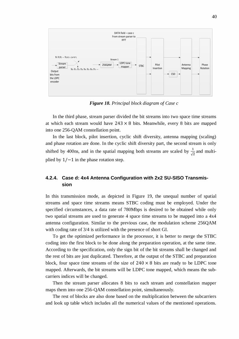
40
Figure 18. Principal block diagram of Case c
In the third phase, stream parser divided the bit streams into two space time streams
at which each stream would have bits. Meanwhile, every 8 bits are mapped
into one 256-QAM constellation point.
In the last block, pilot insertion, cyclic shift diversity, antenna mapping (scaling)
and phase rotation are done. In the cyclic shift diversity part, the second stream is only
shifted by 400ns, and in the spatial mapping both streams are scaled by
√ and multi-
plied by in the phase rotation step.
4.2.4. Case d: 4x4 Antenna Configuration with 2x2 SU-SISO Transmis-
sion
In this transmission mode, as depicted in Figure 19, the unequal number of spatial
streams and space time streams means STBC coding must be employed. Under the
specified circumstances, a data rate of 780Mbps is desired to be obtained while only
two spatial streams are used to generate 4 space time streams to be mapped into a 4x4
antenna configuration. Similar to the previous case, the modulation scheme 256QAM
with coding rate of 3/4 is utilized with the presence of short GI.
To get the optimized performance in the processor, it is better to merge the STBC
coding into the first block to be done along the preparation operation, at the same time.
According to the specification, only the sign bit of the bit streams shall be changed and
the rest of bits are just duplicated. Therefore, at the output of the STBC and preparation
block, four space time streams of the size of bits are ready to be LDPC tone
mapped. Afterwards, the bit streams will be LDPC tone mapped, which means the sub-
carriers indices will be changed.
Then the stream parser allocates 8 bits to each stream and constellation mapper
maps them into one 256-QAM constellation point, simultaneously.
The rest of blocks are also done based on the multiplication between the subcarriers
and look up table which includes all the numerical values of the mentioned operations.
Stream parser
256QAM
DATA field – case cFrom stream parser to
IFFT
Output bits from the LDPC encoder
LDPC tone mapper
Pilot Insertion
AntennaMapping
Stream 1y0 y1y2 … y1872 = 234*8*1
y0, y1, y2, y3, y4, y5, y6, y7, …
Phase Rotation
CSD
STBC
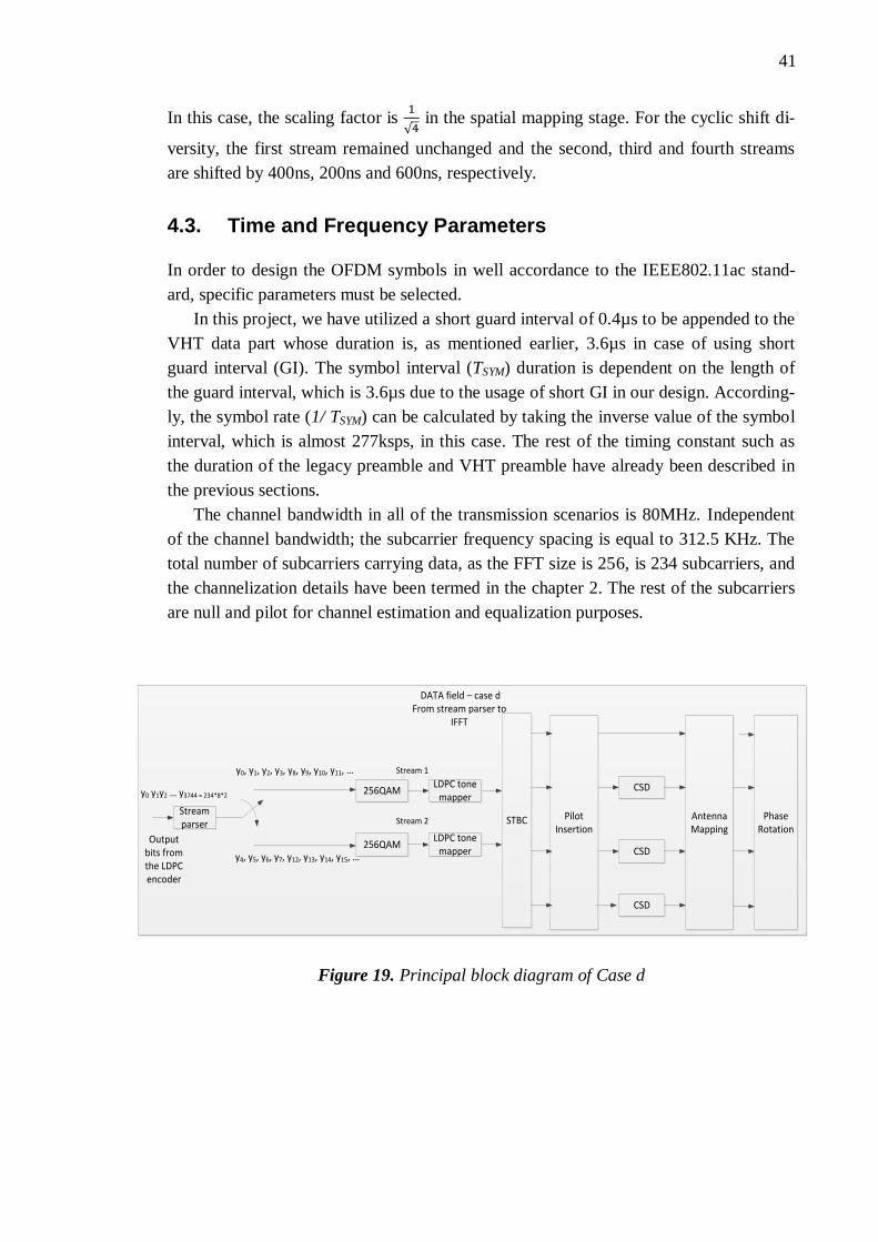
41
In this case, the scaling factor is
√ in the spatial mapping stage. For the cyclic shift di-
versity, the first stream remained unchanged and the second, third and fourth streams
are shifted by 400ns, 200ns and 600ns, respectively.
4.3. Time and Frequency Parameters
In order to design the OFDM symbols in well accordance to the IEEE802.11ac stand-
ard, specific parameters must be selected.
In this project, we have utilized a short guard interval of 0.4µs to be appended to the
VHT data part whose duration is, as mentioned earlier, 3.6µs in case of using short
guard interval (GI). The symbol interval (TSYM) duration is dependent on the length of
the guard interval, which is 3.6µs due to the usage of short GI in our design. According-
ly, the symbol rate (1/ TSYM) can be calculated by taking the inverse value of the symbol
interval, which is almost 277ksps, in this case. The rest of the timing constant such as
the duration of the legacy preamble and VHT preamble have already been described in
the previous sections.
The channel bandwidth in all of the transmission scenarios is 80MHz. Independent
of the channel bandwidth; the subcarrier frequency spacing is equal to 312.5 KHz. The
total number of subcarriers carrying data, as the FFT size is 256, is 234 subcarriers, and
the channelization details have been termed in the chapter 2. The rest of the subcarriers
are null and pilot for channel estimation and equalization purposes.
Figure 19. Principal block diagram of Case d
Stream parser
256QAM
DATA field – case dFrom stream parser to
IFFT
Output bits from the LDPC encoder
256QAM
LDPC tone mapper
LDPC tone mapper
Pilot Insertion
CSD
AntennaMapping
Stream 1
Stream 2
y0 y1y2 … y3744 = 234*8*2
y0, y1, y2, y3, y8, y9, y10, y11, …
y4, y5, y6, y7, y12, y13, y14, y15, …
Phase Rotation
CSD
CSD
STBC

42 42
5. RESULTS AND ANALYSIS
This chapter includes the implementation results which are profiled in the terms of
clock cycles, power and energy consumption and memory usage. In addition, the ob-
tained results will be discussed and compared with some references.
5.1. Software Implementation
In order to program and evaluate the performance of the ConnX BBE32 DSP core, the
Xtensa Xplorer (XX) integrated Development Environment (IDE) is used which is ca-
pable of providing a C/C++ software development workspace. It also offers a compre-
hensive collection of code generation and analysis tools. [51]
However, the utilized processor inherently provides a wide variety of the optimiza-
tion approaches to make the software implementation efficient. As mentioned in the
previous section, appropriate configuration and programming style play an important
role in the efficiency of the implementation, thus some optimization techniques have
been applied in this project to speed up the processing. In principle, everything has been
optimized almost in machine level as the C-code is full of macros, which actually means
that the code is not portable anymore. Another effective optimization approach was
merging and combing the functions as much as possible. Specifically those functions
whose functionality involves multiplication with a constant value, such as phase rota-
tion, spatial mapping, pilot insertion and cyclic shift diversity. Moreover, since it is
easier to deal with bits rather than complex numbers, we have implemented as many
operations as possible before the constellation mapping. For instance, although in the
standard and, as shown in Figure 15, the STBC and LDPC tone mapper blocks are de-
fined to be employed after the 256-QAM modulation; it has been found that such opera-
tions can be efficiently implemented when the input data is still in bits and not yet mod-
ulated to symbols.
5.2. Clock Cycles
To evaluate the processor performance in the term of clock cycle, the instruction set
simulator (iss) is used which determines the needed clock cycles for processing one
OFDM symbol.
The FFT operation needs 311 and 250 clock cycles per OFDM symbol to be done in
LP and PM models, respectively. Table 7 and Table 8 show the previous tables in the
form of bar chart as it is easier to figure out the difference and making comparison.

5. RESULTS AND ANALYSIS 43
0
100
200
300
400
500
600
700
800
900
Case a case b case c case d
Preparation block
LDPC Tone Mapper
Stream parser + ConstellationMapper
Pilot Insertion + CSD + PhaseRotation + Spatial Mapping
Total number of clock cycles
The first transmission has the lowest number of clock cycles, since it has only two
spatial streams without having STBC so that it is the simplest transmission scenario. In
the second transmission scenario, as it was mentioned that the preparation block is not
required be employed so that in Table 7 and Table 8, the preparation clock cycle is
equal to zero. For the third case, as the number of spatial streams was lower than the
number of space time streams the STBC encoder was used. Therefore, in the first block,
in addition to the preparation, the STBC encoding results are reported, That is why the
preparation bar is larger than the other cases.
Similar to the previous transmission mode, in the fourth transmission case, the une-
qual number of spatial streams and space time streams brought up the idea of using
STBC. Consequently, the preparation bar shows both preparation and STBC operations
result. However, due to the similar reason as the second mode, the preparation is not
needed. That is why the number of clock cycles is lower than in the third operation
mode, although the number of spatial streams is higher. The numerical values for all the
transmission scenarios can be found in the Appendix 1.
It is worth noticing that exploiting the PM configuration leads to the lower number
of clock cycles required to execute each transmission mode. As a matter of fact, the
existence of the optional packages accelerates the processing procedure. However, the
speedup is almost negligible, as the additional packages will add some hardware to the
processor and speedup is one few percentages.
Table 7. Clock cycle results in LP model

5. RESULTS AND ANALYSIS 44
0
100
200
300
400
500
600
700
800
900
Case a case b case c case d
Preparation block
LDPC Tone Mapper
Stream parser + ConstellationMapper
Pilot Insertion + CSD + PhaseRotation + Spatial Mapping
Total number of clock cycles
5.3. Power Consumption
One of the most useful performance analysis factors is the power consumption which is,
in this case, dependent on the memory configuration/capacity. As the Energy Xplorer
tool is only able to analyze the energy for each function, first the energy is estimated
and then the power consumption is calculated by dividing the energy values by time.
The time for each block is different and calculated from the multiplication between the
clock cycles and 2ns (the period of each clock cycle or the inverse of frequency). Alt-
hough, the tool provides the total power consumption for each transmission scenario, it
includes all the required power for initialization within the whole run-time.
As mentioned earlier, the memory configuration affects on the power consumption,
so we have considered two common cases which are the maximum (128k) and half
(64k) of the memory capacity. In order to analyze the energy consumption, the 40nm
Low-Power IC technology provided by the vendor is used, and the operation frequency
is assumed to be 500MHz. The monitoring time for the energy analysis is 3.6µs, and the
estimated energy includes both leakage and dynamic parts. In the following, the related
results to the power consumption for each function are reported for PM model, in case
of full and half memory usage. The power consumption results for the PM model are
not presented as they do not differ from the LP model results.
Table 8. Clock cycle results in PM model

5. RESULTS AND ANALYSIS 45
0
1
2
3
4
5
6
7
8
9
case a case b case c case d
Preparation
LDPC Tone Mapper
Stream Parser +Constellation mapper
Pilot Insertion + CSD +Spatial Mapping + PhaseRotation
0
2
4
6
8
10
12
case a case b case c case d
Preparation
LDPC Tone Mapper
Stream Parser +Constellation mapper
Pilot Insertion + CSD +Spatial Mapping + PhaseRotation
It can be concluded from the Table 9 and Table 10 that the second and fourth trans-
mission scenarios have the highest rate of power consumption among the transmission
cases which is due to the existence of four spatial streams for processing.
Table 11 presents the total power consumption for all the transmission scenarios
profiled in the PM configurations and memory capacity of 128K. The same information
is also introduced in Table 12 when the memory capacity is 64K.
Table 9. Power consumption for each function of the transmission scenarios in
mW, 128K
Table 10. Power consumption for each function of the transmission scenarios in
mW, 64K

5. RESULTS AND ANALYSIS 46
0
10
20
30
40
50
60
case a case b case c case d
Processor
Memory
Total
0
5
10
15
20
25
30
35
40
45
case a case b case c case d
Processor
Memory
Total
Table 13 and Table 14 show the total power consumption for all the transmission
scenarios profiled in LP configurations for maximum and half capacity of memory, re-
spectively. As it can be observed, the processor has the highest share in the total power
consumption due to the fact that huge amount of data is processed.
Table 11. Total Power consumption [mW] for PM model in case of full
memory
Table 12. Total Power consumption [mW] for PM model in case of half
memory
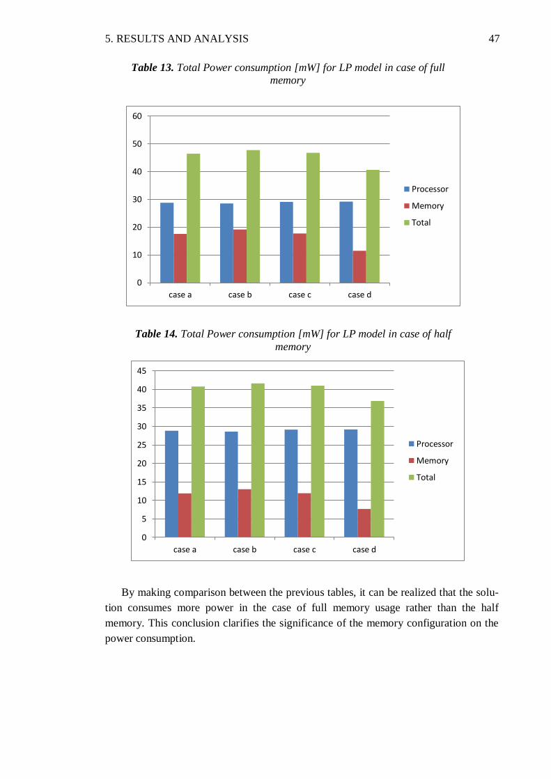
5. RESULTS AND ANALYSIS 47
0
10
20
30
40
50
60
case a case b case c case d
Processor
Memory
Total
0
5
10
15
20
25
30
35
40
45
case a case b case c case d
Processor
Memory
Total
By making comparison between the previous tables, it can be realized that the solu-
tion consumes more power in the case of full memory usage rather than the half
memory. This conclusion clarifies the significance of the memory configuration on the
power consumption.
Table 13. Total Power consumption [mW] for LP model in case of full
memory
Table 14. Total Power consumption [mW] for LP model in case of half
memory

5. RESULTS AND ANALYSIS 48
0
5000
10000
15000
20000
25000
30000
35000
case a case b case c case d
Preparation
LDPC Tone Mapper
Stream Parser +Constellation mapper
Pilot Insertion + CSD +Spatial Mapping + PhaseRotation
0
5000
10000
15000
20000
25000
30000
35000
case a case b case c case d
Preparation
LDPC Tone Mapper
Stream Parser +Constellation mapper
Pilot Insertion + CSD +Spatial Mapping + PhaseRotation
5.4. Energy per Bit
Although in the beginning it was mentioned that the power consumption is better to be
used for analysis, since the Tensilica itself claims that the power conversions are not
very reliable, in the following the energy analysis results are also revealed.
The energy analysis is made for one 3.6µs time frame; the results include both leak-
age and dynamic portions of the energy. As the memory configuration does not have
effect on the results, the memory capacity of 64K is assumed. Table 15 and Table 16
reveal the energy consumption for all the transmission scenarios blocks which are pro-
filed in LP and PM configurations, respectively.
Table 15. Energy consumption [pJ] for each block in all transmission scenarios, LP,
64K
Table 16. Energy consumption [pJ] for each block in all transmission scenarios, PM,
64K
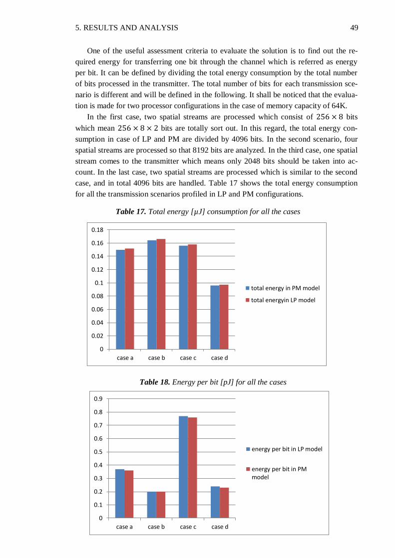
5. RESULTS AND ANALYSIS 49
0
0.1
0.2
0.3
0.4
0.5
0.6
0.7
0.8
0.9
case a case b case c case d
energy per bit in LP model
energy per bit in PMmodel
0
0.02
0.04
0.06
0.08
0.1
0.12
0.14
0.16
0.18
case a case b case c case d
total energy in PM model
total energyin LP model
One of the useful assessment criteria to evaluate the solution is to find out the re-
quired energy for transferring one bit through the channel which is referred as energy
per bit. It can be defined by dividing the total energy consumption by the total number
of bits processed in the transmitter. The total number of bits for each transmission sce-
nario is different and will be defined in the following. It shall be noticed that the evalua-
tion is made for two processor configurations in the case of memory capacity of 64K.
In the first case, two spatial streams are processed which consist of bits
which mean bits are totally sort out. In this regard, the total energy con-
sumption in case of LP and PM are divided by 4096 bits. In the second scenario, four
spatial streams are processed so that 8192 bits are analyzed. In the third case, one spatial
stream comes to the transmitter which means only 2048 bits should be taken into ac-
count. In the last case, two spatial streams are processed which is similar to the second
case, and in total 4096 bits are handled. Table 17 shows the total energy consumption
for all the transmission scenarios profiled in LP and PM configurations.
Table 17. Total energy [µJ] consumption for all the cases
Table 18. Energy per bit [pJ] for all the cases
5. RESULTS AND ANALYSIS 50
Table 18 shows the required energy for transmission of one bit for all the transmis-
sion scenarios. As it can be realized, the third case consumes more energy compared to
the rest which is due to the fact that two spatial streams are processed to generate four
space time streams by using STBC. Therefore, after STBC operations, four streams are
analyzed. However, the second case requires lower energy as it is the simplest case in
the implementation procedure due to the fact that it even does not need the preparation
block in contrast with other scenarios. It is worth noticing that LP and PM configura-
tions results do not considerably differ from each other in this term.
5.5. Memory Usage
One more evaluation parameter is the code size or memory usage. In this project as two
memory categories are used including instruction and data, the evaluation is made for
both of them.
It is worth noticing that among all the listed functions, only LDPC tone mapper and
the last block including pilot insertion, spatial mapping, cyclic shift diversity and phase
rotation are completely loop unrolled. As the loop unrolling increases the code size, the
instruction memory usage for each transmission mode per each operation is presented in
the following tables. Since there is no difference between PM and LP model from the
memory usage point of view, only the results using the PM model are presented.
It should be noted that we have assumed that all incoming bits from the LDPC en-
coder are already stored in the local data memory. The data memory usage for each
transmission mode is also reported at the same tables under ‘input buffer usage’ title,
and it only depends on the transmission scenario.
Table 19 introduces the data and instruction memories usage for the all transmission
mode. It should be noted that the first and second transmission cases does not have
STBC process so that the reported values show only the instruction and data memories
usage for preparation block.
As mentioned earlier, in order to speed up the processing, the numerical values of
the last block including pilot insertion, cyclic shift diversity, spatial mapping and phase
rotation were calculated and stored in a look-up table. This table occupies 128 and 800
bytes from the local data RAM#0 and RAM#1, respectively.
With reference to Table 19, it has been observed that LDPC tone takes more capaci-
ty among the functions. In addition, the amount of used data memory does not depend
on the transmission scenario except for the input buffer usage.
As aforementioned, the utilized processor is an extended version of the Tensilica’s
baseline DSP core and by exploiting additional extension instruction BBE32 will be
configured. Thus, by profiling the total number of instructions (those which are started
by BBE32 prefix) and their code size, useful information will be found out.
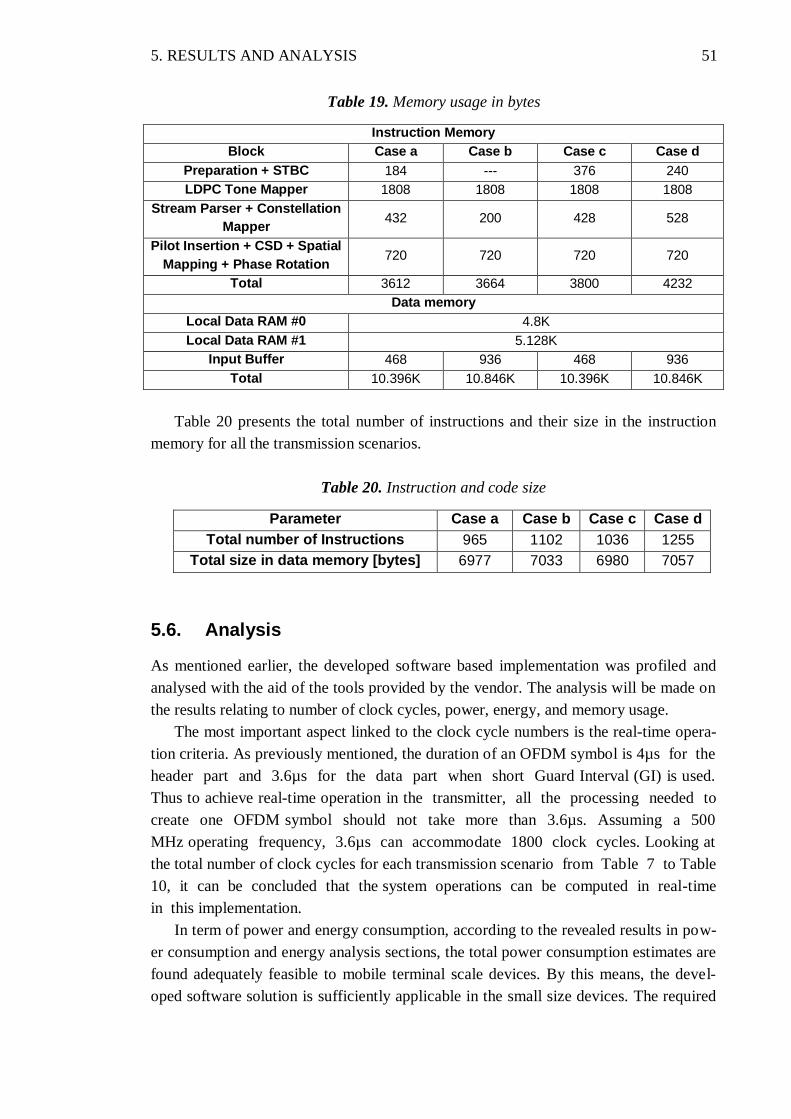
5. RESULTS AND ANALYSIS 51
Table 19. Memory usage in bytes
Instruction Memory
Block Case a Case b Case c Case d
Preparation + STBC 184 --- 376 240
LDPC Tone Mapper 1808 1808 1808 1808
Stream Parser + Constellation
Mapper 432 200 428 528
Pilot Insertion + CSD + Spatial
Mapping + Phase Rotation 720 720 720 720
Total 3612 3664 3800 4232
Data memory
Local Data RAM #0 4.8K
Local Data RAM #1 5.128K
Input Buffer 468 936 468 936
Total 10.396K 10.846K 10.396K 10.846K
Table 20 presents the total number of instructions and their size in the instruction
memory for all the transmission scenarios.
Table 20. Instruction and code size
Parameter Case a Case b Case c Case d
Total number of Instructions 965 1102 1036 1255
Total size in data memory [bytes] 6977 7033 6980 7057
5.6. Analysis
As mentioned earlier, the developed software based implementation was profiled and
analysed with the aid of the tools provided by the vendor. The analysis will be made on
the results relating to number of clock cycles, power, energy, and memory usage.
The most important aspect linked to the clock cycle numbers is the real-time opera-
tion criteria. As previously mentioned, the duration of an OFDM symbol is 4µs for the
header part and 3.6µs for the data part when short Guard Interval (GI) is used.
Thus to achieve real-time operation in the transmitter, all the processing needed to
create one OFDM symbol should not take more than 3.6µs. Assuming a 500
MHz operating frequency, 3.6µs can accommodate 1800 clock cycles. Looking at
the total number of clock cycles for each transmission scenario from Table 7 to Table
10, it can be concluded that the system operations can be computed in real-time
in this implementation.
In term of power and energy consumption, according to the revealed results in pow-
er consumption and energy analysis sections, the total power consumption estimates are
found adequately feasible to mobile terminal scale devices. By this means, the devel-
oped software solution is sufficiently applicable in the small size devices. The required
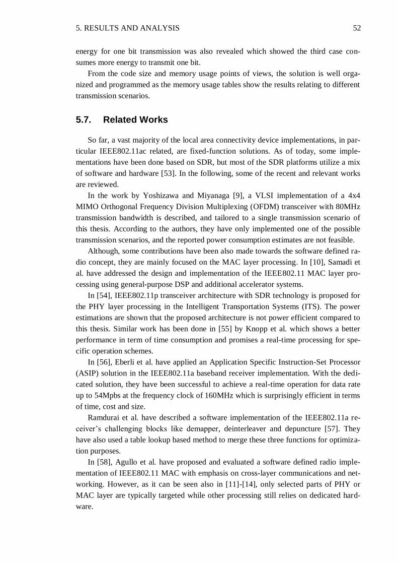
5. RESULTS AND ANALYSIS 52
energy for one bit transmission was also revealed which showed the third case con-
sumes more energy to transmit one bit.
From the code size and memory usage points of views, the solution is well orga-
nized and programmed as the memory usage tables show the results relating to different
transmission scenarios.
5.7. Related Works
So far, a vast majority of the local area connectivity device implementations, in par-
ticular IEEE802.11ac related, are fixed-function solutions. As of today, some imple-
mentations have been done based on SDR, but most of the SDR platforms utilize a mix
of software and hardware [53]. In the following, some of the recent and relevant works
are reviewed.
In the work by Yoshizawa and Miyanaga [9], a VLSI implementation of a 4x4
MIMO Orthogonal Frequency Division Multiplexing (OFDM) transceiver with 80MHz
transmission bandwidth is described, and tailored to a single transmission scenario of
this thesis. According to the authors, they have only implemented one of the possible
transmission scenarios, and the reported power consumption estimates are not feasible.
Although, some contributions have been also made towards the software defined ra-
dio concept, they are mainly focused on the MAC layer processing. In [10], Samadi et
al. have addressed the design and implementation of the IEEE802.11 MAC layer pro-
cessing using general-purpose DSP and additional accelerator systems.
In [54], IEEE802.11p transceiver architecture with SDR technology is proposed for
the PHY layer processing in the Intelligent Transportation Systems (ITS). The power
estimations are shown that the proposed architecture is not power efficient compared to
this thesis. Similar work has been done in [55] by Knopp et al. which shows a better
performance in term of time consumption and promises a real-time processing for spe-
cific operation schemes.
In [56], Eberli et al. have applied an Application Specific Instruction-Set Processor
(ASIP) solution in the IEEE802.11a baseband receiver implementation. With the dedi-
cated solution, they have been successful to achieve a real-time operation for data rate
up to 54Mpbs at the frequency clock of 160MHz which is surprisingly efficient in terms
of time, cost and size.
Ramdurai et al. have described a software implementation of the IEEE802.11a re-
ceiver’s challenging blocks like demapper, deinterleaver and depuncture [57]. They
have also used a table lookup based method to merge these three functions for optimiza-
tion purposes.
In [58], Agullo et al. have proposed and evaluated a software defined radio imple-
mentation of IEEE802.11 MAC with emphasis on cross-layer communications and net-
working. However, as it can be seen also in [11]-[14], only selected parts of PHY or
MAC layer are typically targeted while other processing still relies on dedicated hard-
ware.
5. RESULTS AND ANALYSIS 53
In [59], Iacono et al. have implemented the IEEE802.11a/p receiver based on the
SDR technology. Their main focus is also on the PHY specifications, but the data rate
they have targeted is much lower than our case. Furthermore, the used modulation and
coding schemes also differ which lead to different results. However, the comparison
between the results shows that this project is dominant in terms of clock cycles and
power consumption.

54 54
6. CONCLUSION
In this thesis, the feasibility of the software implementation of the IEEE802.11ac trans-
mitter frequency domain baseband processing is studied. Our main focus was on the
PHY layer implementation in four different multiantenna operation points which in-
clude 2x2 and 4x4 MIMO antenna configurations to achieve a data rate beyond 1Gbps.
The employment of the higher number of spatial streams up to 4 streams, higher modu-
lation order like 256-QAM scheme and wider bandwidth of 80MHz resulted in massive
amount of data processing which can be carried out by the utilized DSP, ConnX
BEE332.
The analysis of the performance numbers clearly shows that the developed software
based implementation on a DSP core can achieve real-time operation for the transmitter
baseband processing assuming 500 MHz clock frequency. Furthermore the implementa-
tion resulted in realistic power consumption and memory usage, despite of massive
amount of data processing yielding beyond 1Gbps transmission bit rate in the most am-
bitious transmission scenario. In terms of power, as the power consumption estimates,
in Chapter 5, showed the maximum value of 40mW; therefore, the proposed software
implementation is found feasible to the mobile terminal scale devices.
Regarding the programmable SDR application in the baseband processing, it can be
stated that the vector processors are well promising cores for scalable, flexible and
adaptable parallel processing a huge amount of data. Consequently, in order to deal with
newer wireless standards and multi operational standards devices, exploiting the vector
processor is probably an appropriate choice to achieve low power consumption and cost
to compete with other venders. However, flexibility, compatibility, and adaptability can
be solved with programmability, performance calls for certain processors. The perfor-
mance can be increased by customizing the processor according to the needs of the ap-
plication. If the application has inherent data parallelism, then vector processing or
SIMD extensions can be used which are capable to provide energy-efficiency compared
to general-purpose processor without customizations.
It is worth noticing that the software based implementation for the transmitter only
includes the frequency domain PHY functions, in other words it does not provide the
MAC layer functions and non-frequency domain functions such as IFFT. However, in
order to provide a competitive implementation in the terms of power and area, both
hardware and software designs need to be defined and assessed. In addition, the accura-
cy of the power and energy measurements is not certain and determined which lead to
error in the results and evaluation. In order to measure the power, the platform must be
implemented on the chip which is not done in this research. In the real-time evaluation,

55
we have not taken into account the time needed to receive all the data in the local mem-
ories. In fact, it has actually been assumed that all the data are already stored in the local
data memories; hence the required time for data transfer to the local memory has not
been considered.
In this thesis, we have also found that the customized VLIW processors with the
vector processing capabilities provide highly improved flexibility, much faster time-to-
market and more possibilities to bringing in new transmission features and enhance-
ment. Meanwhile, the compatibility and adaptability problems in the conventional
fixed-function modems can be conquered. As a result, by the rapid pace of wireless
communications systems growth, we can be hopeful that the software based implemen-
tation can be upgraded. Thus, the entire system does not need to be replaced.
The future work will focus on implementing the corresponding receiver chain PHY
processing which includes computationally more intensive processing such as channel
state estimation and detection.
56 56
REFERENCES
[1] D. Tse, P. Viswanath, Fundamental of Wireless Communications, Cambridge Uni-
versity Press, 2005.
[2] L. Cinquino, A., R. Shayan, Y., A Real-Time Software Implementation of an
OFDM Modem Suitable for Software Defined Radio, IEEE, 2004.
[3] IEEE Standard for Information Technology‒Telecommunications and Information
Exchange between Systems and Local and Metropolitan Area Networks‒Specific
Requirements. Part 11: Wireless LAN Medium Access Control (MAC) and Physical
Layer (PHY) Specifications, IEEE Std 802.11TM
, 2012.
[4] Quatenna Communications, An Introduction to IEEE802.11ac, Sigurd Schelstraete,
September 2013.
[5] R. Berger, C., Arbatov, V., Voronenko, Y., Franchetti, F., Puschel M., Real-Time
Software Implementation of an IEEE802.11a Baseband receiver on Intel Multicore,
ICAPP, 2011.
[6] Wolf, W., Building the Software Radio, Computer, Vol. 38, No. 3, March 2005.
[7] Koch, P., Prasad, R., The Universal Handset, IEEE Spectrum, Vol. 46, No. 4, April
2009.
[8] V. Berkel, K., Heinle, F., P. E. Meuwissen, P., Moerman, K., Wiess, M., Vector
Processing as an Enabler for Software Defined Radio in Handheld Devices, EURA-
SIP Journal on Applied Signal Processing, 2005.
[9] S. Yoshizawa and Y. Miyanaga, VLSI Implementation of a 4×4 MIMO-OFDM
transceiver with an 80-MHz channel bandwidth, in Proc. ISCAS, Taipei, Taiwan,
24-27 May 2009, pp. 1743-1746.
[10] S. Samadi, A. Golomohammadi, A. Jannesari, M.R. Movahedi, B. Khalaj, and
S. Ghammanghami, A Novel Implementation of the IEEE802.11 Medium Access
Control, in Proc. Int. Symp. Intelligent Signal Process. Commun., Yonago, Japan,
12-15 Dec. 2006, pp.489-492.
[11] K. Rounioja, and K. Puusaari, Implementation of an HSDPA Receiver with a
Customized Vector Processor, in Proc. Int. Symp. System-on-Chip, Tampere, Fin-
land, 13-16 Nov. 2006, pp. 1-4.

57
[12] W. Xu, M. Richter, M. Sauermann, F. Capar, and C. Grassmann, Efficient
baseband implementation on an SDR platform, in Proc. Int. Conf. ITS Telecom-
munications, St. Petersburg, Russia, 23-25 Aug. 2011, pp.794-799.
[13] J. Janhunen, T. Pitkänen, M. Juntti, and O. Silvén, Energy-efficient program-
mable processor implementation of LTE compliant MIMO-OFDM detector,” in
Proc. ICASSP, Kyoto, Japan, 25-30 March 2012, pp. 3276 – 3279.
[14] S. Eberli, A. Burg, and W. Fichtner, Implementation of a 2×2 MIMO-OFDM
Receiver on an application specific processor, Microelectronics Journal, vol. 40, No.
11, pp. 1642-1649, November 2009.
[15] IEEE global history network, Wireless LAN 802.11 Wi-Fi.
[16] IEEE Standard Association [WWW]. [Accessed on 20.11.2013]. Available at:
[http://standards.ieee.org/about/ieeesa.html]
[17] Agilent Technologies, IEEE802.11Wireless LAN PHY Layer (RF) Operation
and Measurement, USA, April 2002.
[18] IEEE Standard for Information Technology‒Telecommunications and Infor-
mation Exchange between Systems and Local and Metropolitan Area Networks‒
Specific Requirements. Part 11: Wireless LAN Medium Access Control (MAC) and
Physical Layer (PHY) Specifications, IEEE Std 802.11TM
, 2013.
[19] IEEE 802.11 WG, part 11a/11b/11g, Wireless LAN Medium Access Control
(MAC) and Physical Layer (PHY) specifications, Standard Specification,
IEEE,1999.
[20] Eldad Perahia and Intel Corporation, IEEE802.11n Development: History, pro-
cess, and Technology, July 2008, IEEE communications magazine.
[21] Mamshaei, M. H., Cantieni, G. R., Barakat, C., Turletti, T., Performance Analy-
sis of the IEEE802.11 MAC and PHY Layer Protocol, IEEE, June 2005.
[22] Valadas, R.T., Tavares, A.R., Duarte, A.M.deO., Moreira, A.C., Lomba, C.T.,
The infrared physical layer of the IEEE 802.11 standard for wireless local area net-
works, Communications Magazine, IEEE , vol.36, no.12, pp.107-112, Dec 1998.
[23] Pahlavan, K., H. Probert, T., E. Chase, M., Trends in Local Wireless Networks,
IEEE Communications magazine, March 1995.
58
[24] Aftab Ahmad, Data Communication principles: for fixed and wireless networks,
2003, Kluwer Academic Publisher.
[25] Roshan, P., Leary, J., IEEE802.11 Wireless LAN Fundamentals, Indianapolis
2003, Cisco Press.
[26] IEEE802.11b Wireless LANs; Wireless Freedom at Ethernet Speeds, Technical
Paper, 3COM Corporation.
[27] Perahia, E., Stacey, R., Next Generation Wireless LANs Throughput, Robust-
ness, and Reliability in 802.11n, Cambridge University Press, 2008, Chapter 7.
[28] Eldad Perahia, Robert Stacy, Next Generation Wireless LANs, Cambridge, 2nd
edition, 2013.
[29] Mohinder Jankiraman, Space-Time Codes and MIMO Systems, 2004, ARTECH
House.
[30] IEEE 802.11 WG. International standard for information technology – local and
metropolitan area networks, part 11: wireless LAN MAC and PHY specifications,
1999.
[31] Sylvester, A. U., Prince, A. O., Edward, O. E., Carrier Sensing Mechanisms:
The Impact on Throughput Performance of IEEE 802.11WLANs, Scholar, Vol. 1,
No. 1,March 2012.
[32] Zheng Y., Lu k., Wu D., Performance analysis of IEEE 802.11 DCF in
imperfect channels, ACM conference 2002.
[33] P. Crow, B., Widjaja, I., Geun Kim, J., T. Sakai, P., IEEE802.11 Wireless Local
Area Networks, IEEE Communications Magazine, Spetember 1997.
[34] IEEE Standard 802.11-2007, Wireless LAN Medium Access Control (MAC)
and Physical Layer (PHY) Specifications, June 2007.
[35] Sikdar, B., Delay analysis of IEEE 802.11 PCF MAC based wireless networks,
Global Telecommunications Conference, 2005. GLOBECOM ’05. IEEE , vol.1, 28
Nov.-2 Dec. 2005.
[36] Prasad, R., J. Velez, F., OFDM WI-MAX Physical Layer, Springer, 2010.
[37] Qualcomm, IEEE802.11ac The next evolution of Wi-Fi standards, May 2012.
59
[38] Roche, G., Glazunov, A. A., Allen, B., LTE-Advanced and Next Generation
Wireless Networks: Channel modeling and propagation, Wiley, 2013.
[39] Aruba White Paper, 802.11ac In-Depth,.
[40] Tensilica Inc., ConnX BBE32 DSP user guide, USA, 2012.
[41] Fosdick, D., R. Jessup, L., J. C. Shauble, E., Domik, G., An Introduction to High
Performance Scientific ComputingThe Massachusetts Institute of Technology, 1996.
[42] Asanovic, K., Vector Processors, Elsevier Science, 2003.
[43] Flynn, M. J., Computer Architecture: Pipelined and Parallel Processor Design,
Jones and Bartlett Publisher, 1995.
[44] L. Null, J. Lobur, Computer Organization and Architecture, Jones and Bartlett
Publisher, 2006.
[45] Jadhav, S. S., Advanced Computer Architecture and Computing, Technical Pub-
lication Pune, 2009.
[46] J., Dongarra, J., Hernandez, V., Vector and Parallel processing, VECPAR’98.,
Palma, Springer, 1998.
[47] Censor, N., Parallel Optimization: Theory, Algorithm, and Application., 1997,
Oxford.
[48] NVIDIA SDR Technology, The modem innovation inside NVIDIA i500 and
Tegra 4i, 2013.
[49] Saksena, M., Selic, B., Real-Time Software Design- State of the Art and Future
Challenges, IEEE Canadian Review, Summer 1999.
[50] Tensilica Inc., ConnX BBE32 DSP Core for Baseband Processing, Configura-
ble, Extensible and Scalable, USA, March 2013.
[51] Tensilica Inc., ConnX BBE32 DSP Core for Baseband Processing, USA, 2013.
[52] Draft Standard for Information Technology‒Telecommunications and Infor-
mation Exchange between Systems and Local and Metropolitan Area Networks‒
Specific Requirements. Part 11: Wireless LAN Medium Access Control (MAC) and
Physical Layer (PHY) Specifications. Amendment 4: Enhancement for Very High
60
Throughput for Operation in Bands below 6GHz. IEEE P802.11acTM
: D5.0, New
York, January 2013.
[53] Anjum, O., Ahonen, T., Garzia, F., Nurmi, J., Brunelli, C., Berg, H., State of the
art baseband DSP platforms for softwaredefined radio: a survey, EURASIP Journal
on Wireless Communications and Networking, 2011, 5.
[54] Chen, Y.-H., A novel multicore SDR architecture for smart vehicle systems,
Proc. of the 12th Int. Conf. on Intelligent Transport Systems Telecommunications
(ITST), November, 2012.
[55] Schmidt-Knorreck, C., Knorreck, D., Knopp, R., IEEE 802.11p receiver design
for software defined radio platforms, DSD 2012, 15th Euromicro Conference on
Digital System Design, 5 – 8 September, 2012, Cesme, Izmir, Turkey.
[56] Eberli, S., Burg, A., Bösch, T., & Fichtner, W., An IEEE 802.11a baseband re-
ceiver implementation on an Application Specific Processor, Proceedings of IEEE
Midwest Symposium on circuit & Systems, Montreal, Quebec, Canada, pp. 1324 –
1327, Aug 2007.
[57] Ramadurai, V., Jinturkar, S., Agarwal, S., Moudgill, M., Glossner, J., Software
Implementation of 802.11a blocks on Sandblaster DSP, Proceedings of Software
Defined Radio Technical Forum, Orlando Florida, November, 2006.
[58] J.R. Gutierrez-Agullo, B. Coll-Perales, J. Gozalvez, An IEEE 802.11 MAC
Software Defined Radio implementation for experimental wireless communica-
tions and networking research, in Proc. IFIP Wireless Days, Venice, Italy, 20-22
Oct. 2010, pp.1-5.
[59] Lo Iacono, D., Cupaiuolo, T., Power Efficient SDR Implementation of
IEEE802.11a/p Physical Layer, Springer, 2013.
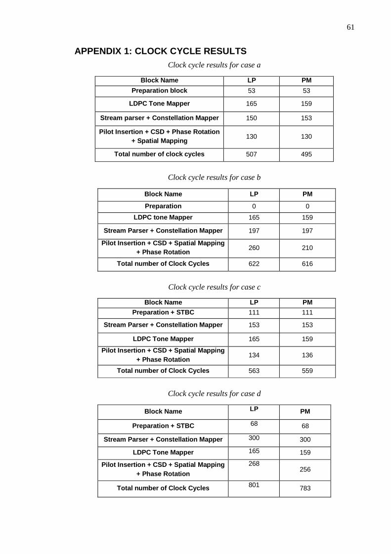
61
APPENDIX 1: CLOCK CYCLE RESULTS
Clock cycle results for case a
Block Name LP PM
Preparation block 53 53
LDPC Tone Mapper 165 159
Stream parser + Constellation Mapper 150 153
Pilot Insertion + CSD + Phase Rotation
+ Spatial Mapping 130 130
Total number of clock cycles 507 495
Clock cycle results for case b
Block Name LP PM
Preparation 0 0
LDPC tone Mapper 165 159
Stream Parser + Constellation Mapper 197 197
Pilot Insertion + CSD + Spatial Mapping
+ Phase Rotation 260 210
Total number of Clock Cycles 622 616
Clock cycle results for case c
Block Name LP PM
Preparation + STBC 111 111
Stream Parser + Constellation Mapper 153 153
LDPC Tone Mapper 165 159
Pilot Insertion + CSD + Spatial Mapping
+ Phase Rotation 134 136
Total number of Clock Cycles 563 559
Clock cycle results for case d
Block Name LP PM
Preparation + STBC 68 68
Stream Parser + Constellation Mapper 300 300
LDPC Tone Mapper 165 159
Pilot Insertion + CSD + Spatial Mapping
+ Phase Rotation
268 256
Total number of Clock Cycles 801
783