NOAA Technical Report NOS 114 Charting and Geodetic Services Series CGS 7

Coordinate Conversion for Hydrographic Surveying

Richard P. Floyd

National Charting Research and Development Laboratory

Rockville, MD

December 1 985

u.s. DEPARTMENT OF· COMMERCE National Oceanic and A�mospheric Administration National Ocean Service

NOAA Technical Report NOS 114 Charting and �eodetic Services Series CGS 7

Coordinate Conversion for Hydrographic. Surveying

Richard P. Floyd

National Charting Research and Development Laboratory

Rockville, MO December 1 985 Reprinted August 1986 Reprinted August 1987 �rinted November 1994

u.s. DEPARTMENT OF COMMERCE M.lcolm a.ldrlge, Secre.ry National Oceanic and Atmospheric Administration Anthony J. Cello. Administrator

. National Ocean Service Paul M. WOlff. Assistant Administrator

. Charting and Geodetic Services R. Adm. John D. Bossler. Director

Ment10n of a commerc1al company or product does not constitute an endorsement by the U.S. Government. Use for pub11c1ty or advert1zing purposes of information from this publ ication concern1ng proprietary products or the tests of such products 1"S not authorized.

11

CONTENTS

Acknowledgement • • • • • • • • • • • • • • • • • • • • • • • • • • • • • • 1v Abstract • • • • • • • • • • • • • • • • • • • • • • • • • • • • • • • • • 1 Introduction • • • • • • • • • • • • • • • • • • • • • • • • • • • • • • • 1

Background • • • • • • • • • • • • • • • • • • • • • • • • • • • • • • • 1 Scope • • • • • • • • • • • • • • • • • • • • • • • • • • • • • • • • • • 2 Tenni no logy • • • • • • • • • • • • • • • • • • • • • • . • • • • • • • • • 3

Planar coordinates and their reference systems • • • • • • • • • • • • • • 3 Coordinates and origins • • • • • • • • • • • • • • • • • • • • • • • • • 3 Scale . . . . . . . . . . . . . . . . . . . . . . . . . . . . . . . . . . 4 State Plane Coordinate Syst� • • • • • • • • • • • • • • • • • • • • • • 5

Accuracy • • • • • • • • • • • • • • • • • • • • • • • • • • • • • • • • • 6 Exact coordinate conversion • • • • • • • • • • • • • • • • • • • • • • • 6 Practical coordinate conversion accuracies • • • • • • • • • • • • • • • 6

Coordi nate conversion procedures • • • • • • • • • • • • • • • • • • • • • 7 Coordinate transfonnation algorithms • • • • • • • • • • • • • • • • • • • 8

Isometric latitude • • • • • • • • • • • • • • • • • • • • • • • • • • • 8 Inputs and outputs • • • • • • • • • • • • • • • • • • • • • • • • • • • 9 Synabo 1 091 • . • . . . • . • • • . . . • . • • . • . • . . . . . . . . . . 9 Normal Mercator projection • • • • • • • • • • • • • • • • • • • • • • • 10 Transverse Mercator projection • • • • • • • • • • • • • • • • • • • • • 16 Oblique Mercator projection • • • • • • • • • • • • • • • • • 24 Lambert confonnal conic projection • • • • • • • • • • • • • • • • • • • 33 Polyconi c projection • • • • '. • • • • • • • • • • • • • • • • • • • 41 Azimutha·l equidistant projection • • • • • • • • • • • • • • • • • • • • 49 Datum transformation • • • • • • • • • • • • • • • • • • • • • • • • • • 56

Appendi ces A. El l i psoi d parameters • • • • • • • • • • • • • • • • • • • • • • • • 63 B. State Plane Coordinate System of 1927 prOjection parameters • • • • • 64 C. XVZ coordinate transl ation parameters • • • • • • • • • • • • • • • • 72 D. FORTRAN subroutines • • • • • • • • • • • • • • • • • • • • • • • • • 75 E. Test points • • • • • • • • • • • • • • • • • • • • • • • • • • • • • 105

References • • • • • • • • • • • • • • • • • • • • • • • • • • • • • • • • 119

i11

ACKNOWLEDGEMENT

I thank Ruby L . Becker, of the National Charting Research and Development Labroratory. for coding the subroutines, hel pi ng to debug them , and ass i sting me i n proofreadi ng the manuscript. Her work was inval uable in making this an accurate document.

COORDINATE CONVERSION FOR HYDROGRAPHIC SURVEYING

Richard P. Fl oyd National Charting Research and Development Laboratory

Nat10nal Ocean Service , NOAA Rockvi l l e , Maryl and

ABSTRACT: Hydrographic survey pos itional data are processed , reported , and pl otted using a variety of coordinate systems . Geodetic coordinate systems (latitude and longi tude ) provide worldwide coverage on reference surfaces that cl osely approximate the physical Earth . They form a bas i s upon which pl anar coordi nate systems 'are founded. Planar systems are used extensively for the ir conceptual s impl icity and their ·cartographic . appl i cations .

Information from various sources must be referenced to a common coordinate system before i t can be rel ated. Coordi nate conversions , invol ving one or more coordinate transformations , are used to reduce coordinates to a common system. Thi s report contai ns a general procedure for performing a coordinate conversion and detail ed a lgorithms for making coordinate transformations. Expl anations of various planar projections and l imitations on their use are given.

INTRODUCTION

Background

Pl otting soundings and features to al l ow comparison of historical wi th contemporary survey data i s an important aspect of hydrographi c surveyi ng. In order to accompl i sh these tasks , i t i s necessary to reduce the pOSitions associated with the i nformation to a common frame of reference . Positional reference systems can be categorized into three broad groups : geodetic (al so cal led geographi c ) i n which coordinates are given i n terms of a curvil i near l atti ce of l ati tudes and 10n9itudes; pl anar , i n whi ch coordinates are g iven i n terms of a recti l i near l atti ce of XiS and yls , northings and eastings , or l atitudes and departures; and space , in which coordi nates are given in terms of a Cartesian system of XiS , YIS , and lis .•

The measurements obtai ned to determine positions are made relative to the physical Earth , as characterized by i ts topography and by an undulati ng , semiphysical surface cal l ed the geoid , whi l e the computations required for determining position must be based on a mathematical ly definable reference system. For geodetic coordinates , the mathematical reference system i s the surface of an e l l ipsoid of specified' s ize and .shape , oriented to the surface of the Earth in a manner defi ned by the geodeti c datum. Lati tude and l ongi tude are determined by projecting the point i n question from its physical l ocation to· the el l ipsoid , al ong a l i ne normal to the el l i psoid . Pl anar coordinates are determined s imilarly; i .e . , poi nts are projected from thei r physical l ocation onto a mathematical ly defined reference pl ane or devel opable

1

surface. (A devel opabl e surface is one having curvature i n only one di rection. such as a cone or cyl inder. which can be "rol led out" wi th no angular or l i near distortion i nto a plane. ) Usual ly, .poi nts are projected from the ir physical .l ocation onto a geodetic surface. then projected from the geodetic surface to the pl ane or devel opable surface. Such a doubl e projection may not be immediately apparent. Space coordinates depend only on the l ocation of the coordinate origin and the orientation of the coordi nate axes. Poi nts 'are not projected onto a' surface. as they are i n geodetic and . pl anar reference systems. Usual ly the space coordinate origin coincides with the center of a conventional el l ipsoi d.

:The el l ipsoid cl osely approximates the geoidal surface of the Earth. Thus , there is l ittle difference between angles and distances measured on the topographic surface of the Earth and thei r geodetiC counterparts . represented on the el l ipsoid. Any distortions are caused principal ly by i rregul arities· i n the gravity fiel d as refl ected i n the geoid. Si�i.l arly , distortions between measured quantities and thei r counterparts . in a spatial coordinate system are caused primarily by geoi,dal . undul ations . On the other hand,· planar coordinates are tied to a frame . of' reference that is further from physical rea11ty . Angles and di stances measured on the Earth acqui re greater distortion when represented i n a planar system ·than when represented i n a geodetic or a spatial system.

This discussion focuses on the fol l owing important concepts: ( 1 ) Distortions between measured and projected angl es and distances can be mathematical ly accounted for regardless of the reference system empl oyed , but distortions i n a pl anar system are of greater magnitude and requi re more l engthy computations. (2) The el l ipsoid i s often used as an i ntenmediate surface when projecting poi nts from the physical surface of the Earth to a pl ane surface. ·

·{.Hi storical hydrographic positional data might be referenced to one of several geodetic datums or to a great variety of pl anar reference systems. Coordinate conversions must be empl oyed as requi red to �present a l l positions on a common basis before the information associated with ·the pOSitions can be compared.

Scope

An automated hydrographic data acquisition and processi ng system must be capable of a variety of tasks requi red by the surveyor. Coordinate conversi ons i s one such task . I n converting coordinates from one reference system to another , one or more operations cal led "coordinate transformations" are requi red . The al gori thms provided i n thi s report are for those transformations . Subroutines coded from the a lgori thms, .. havi ng both cartographic and survey appl ications , woul d l ie at the l owest l evel of programming i n an automated system. Transformation a lgori thms are provided for differing geodetic datums and for the fol l owing mapping prOjections:

1 . Normal Mercator 2. Transverse Mercator 3 . Oblique Mercator 4. Lambert conformal conic 5. Polyconic 6·. Azimuthal equ idi stant

2

Terminol ogy

Coordinate conversion·is used in a general sense in this report to denote the process of· changing the coordi nates of a position represented i n one reference system to the coordi nates of that position represented i n any other reference system. Coordinate conversions i nvol ve one or more coordi nate transformations . .

Coordinate transformation appl ies specifical ly to the process of converti ng geodetic coordinates to planar coordi nates based on the same elli psoid (forward transformation ), converti ng planar coordinates to geodetic coordi nates based on the same el l i psoi d (inverse transformation ), and converting geodeti c coord inates to geodetic coordinates based on a d ifferent el l i psoi d (datum transformation ) . Transformations are bas i c operations i n performing the more general coordi nate conversions .

A mapping projecti on. or s imply projection , i s a system whereby geodeti c coordinates and planar coordi nates are related w ith a one-to-one correspondence. (Note that the tenn "projection" appl ies here to mappi ngs between mathemati cal surfaces, not to the projection of a poi nt on the phys i cal surface of the Earth to.a mathematical surface . ) Mappi ng projections are defi ned by specifyi ng certai n conditions that must be met. When a projecti on i s referred by name, those condi tions are i mpl ied . For exampl e. i n the transverse Mercator projection. angl es between i nfin ites imal l i ne segments are preserved, and scale i s hel d constant al ong a selected meridian . Mappi ng projections are further defined by spec ifying certai n projection parameters, thereby orienti ng the pl ane or devel opable surface to the el l i psoid . For instance. a specifi c transverse Mercator projecti on i s defi ned by speci fying the central meridian at 900 west l ongi tude, where scale factor equal s 1 (exactly ) . Most preci sely, a mapping projection is defined by i ts mappi ng equations. whi ch are used to make the one-to-one correspondence between coordinates . Mappi ng equations cou ld be left i n cl osed, exact form, but approximati ons must be i ncorporated to enable the computation of numeri cal resul ts . Di fferent mathematic ians have used different approximations, yiel ding sl i ghtly di fferent resul ts (even though a one-to-one correspondence i s ma i ntai ned us ing a particu lar set of equations ) .

PLANAR COORDINATES AND THEIR REFERENCE SYSTEMS

Coordi nates and Ori gins

Two types of pl anar coordi nates and three pl anar coordi nate ori gi ns are of i nterest i n thi s report. "True" coordinates are those reckoned from the true ori g i n of the projection . They are at a scale i nherent wi th the ·projection, a scale dictated by the projection parameters . "Grid" coord inates are at the same i nherent scale, but are referenced to an orig i n s ituated more conveniently for a parti cular area of i nterest. The true ori g in i s the fundamental orig i n of the projection. lying at a poi nt that ori ents the prOjecti on surface with the g'l obe. Nonnal ly the gri d ori gir, i s l ocated by desi gn to the west and south of the region of i nterest (or "zone" ), so. that resulti ng grid coordi nates are posi ti ve-val ued and 01 a des i red magni tude .

3

A thi rd origi n , termed "fa lse ori g in" i n this report , is sometimes used as an i ntermediate ori g in when goi ng from a, true orig in to a grid orig in . The use of a fal se orig in is strictly to, faci l itate the understanding of the transl ation of coordinates from the true origin to the grid orig i n; it has no ' other �ign�fi cance . Under certai n ci rcumstances , the fa l se origi n cou l d be co10cated with either the true orig in or the grid ori gi n . ' False easti ngs and fa'1se north i ngs are x and y val ues used in the transl ation of coordi nates from one ori g in to another. They can be thought of as coordinates i n the gri d s1stem that are aSSi gned to the true orig in or to the fa lse orig in . .

Scal e

'Sca1e , i n the context of this report , is the ratio ' of distance over the projection surface to distance over the reference el l i psoi d (geodeti c distance ) . It i s a quantity not cl early understood by many. Except along certain specific lines on some projections. scale varies from point to point. In general, scale even var1es w1th d1rection from a poi nt . In conformal map projections scale . is i ndependent of di rection , though i t,i s sti l l dependent on position. PrOjections used for 's�rveying are usually conformal . .

·Li nes al ong whi ch scale mi ght be hel d constant are specified by the projection parameters'. For example , on the 'transverse Mercator projection , scale is constant a long the centra l meridian . On the Lambert conformal conic projection , sca le is constant al ong paral lel s , al though it general ly differs from any gi ven paral lel to another. When scal e is speci fied for a prOjection , it- i s impl ied , . i f not expl i citly stated , a long those speci�ic l i nes .

The magnitude of a speci fied scale factor is near unity i f the projection is to be used for survey coordi nates . For ca�tographic appl i cations, the specified scale factor is a small number, for example 1/10,000 or 1/250,000. B�ar i n mi nd that al though the magnitudes ' of survey and cartographic scale factors are widely separated , they represent the same thi ng i n essence . A speci fied cartograp.h ic sca le factor appl ies. to a spec, ific 1 i ne or poi nt on the geodeti c reference 'el l i psoi d j ust as a spec'i fi ed survey stale factor does. . One must be careful when i nterpreti ng cartographic scale factors .

Consi der the fol l owi ng scenari o. Pl ane survey coordinates are computed on a given projection having a scale factor of 0 . 9996 along its central line . The survey coordinates are then reduced by 1/10.000 to be pl otted on a map . Subsequently , a n i nverse transformation is performed on the map coordinates. to obtai n geodeti c coordi nates for the survey poi .nts. Usi ng a scale factor of 1/10 ,000 along the central li ne of the projection wi l l result i n substantial error in the computed geodeti c coordinates. In this scenari o , the sca le factor that shoul d have been used is 0 . 9996(1/10 ,000 ) , or about 1110 ,004. If , on the other hand , map coordi nates for the survey poi nts had been orig inal ly computed di rectly from geodetic coordi nates , the scale factor of 1/10 ,000 i n the i nverse transformation wou ld have been correct.

4

State Plane Coordinate System

The State Pl ane Coordi nate System of 1927 (so cal l ed because it i s based on the North Ameri can Datum of 1927 ) was dev i sed by the U . S . Coast and Geodeti c Survey (C&GS) i n the 1930's . Its purpose was to al l ow surveyors and engineers to compute accurate coordi nates using pl ane tri gonometry. Corrections to observed angles and di stances are made to account for di screpancies between pl anar and el l i psoi dal computations . Original ly, tabl es of constants that were computed by the C&GS using common l ogarithms were pr.ovided to simpl i fy cal culation of positions . Later, Cl ai re (1973 ) of the C&GS provi ded algorithms and constants for machine computation of pos itions. These al gorithms were designed to dupl icate resul ts obtai ned using the tabl es . For that reason, they are purposely i naccurate to a s l i ght " degree.

" "

The State Pl ane Coordi nate System of 1983 (so called because it is based on the North Ameri can Datum of 1983) was necessitated by the 1983 adjustment of the North Ameri can Datum. Mappi ng equations used by the National Geodetic Survey (NGS ) of the National Ocean Service , National Oceanic and Atmospheri c Admini stration , for transformation between 1983 coordi nates provide very accurate resul ts . Several of the al gorithms i n thi s report make use of the NGS equations , and shou ld produce identi cal resul ts . They wi l l not produce results identical to the C&GS al gorithms for 1927 coordinates . However, s i nce the preval ent use of 1927 coordinate transformations woul d be i n the i nverse mode. it is more appropriate to obtain as accurate a transformation as possible than to dupl i cate the C6GS al gorithms .

Projection parameters for the State Pl ane Coordi nate System of 1927 were publ icized i n Mitchel l and Simmons (1945 ) . Some ambiguity cou ld arise from using those parameters l i sted for the Lambert conformal conic zones due to the fact that mutual ly excl usive parameters are gi ven . State pl ane coordi nate zones us ing the Lambert conformal conic projection are defined with north and south standard paral l el s . The central paral lel and its associated scal e found 1n the Mitchel l and Simmons are deri ved quantities, maki ng them approximate val ues that shou ld not be used for computations. Appendix B of thi s report contai ns the correct parameters for the State Pl ane Coordi nate System of 1927 .

The State of Michigan requ ires special attention . It was original ly gi ven three zones based on the transverse Mercator projection . In 1964 the Michigan coordi nate system was revi sed to consist of three zones based on the Lambert conformal conic projection rai sed to an elevation of (nomi nal ly ) 800 U.S. survey feet. The coordinate system el evated to that height i s equ i valent to a system at "sea l evel" on an el l i psoid with equival ent fl attening , but wi th a semimajor axi s defined as exactly 1 . 0000382 times the conventional semimajor axi s (Berry 1971 ) . Carryi ng out the multipl i cation , the semimajor axi s for the 1964 Michi gan coordinate system i s 6,378 ,450. 04748448 meters , exactly.

5

ACCURACY

Exact Coordi nate Conversion

Cons ider the process by which field observati ons are used to compute coordi nates . The basic steps are the same, i rrespecti ve of the coordinate system employed . Fi rst, measurements such as di stances and angl es are corrected for systemati c errors attributabl e to the measuri ng system. lnstrument error correcti ons account for errors di rectly attributabl e to the measuri ng equ i pment. Envi ronmenta l corrections account for fl uctuations i n a measured val ue due to the effect that envi ronmenta l fl uctuations have on the measuri ng i nstrument. Second, the corrected measurements are IIreduced" (changed, not necessari ly made smal ler) to a common surface on whi ch coordi nate computati ons can be made . And thi rd, mathemati cal model s' based on geometric relationships are used to detennine coordinates of unknown positions from those of known positions using the reduced measurements . Converti ng the coordinates thus obtained to coord"inates in a different reference system can be accompl i shed i n a straightforward manner by applyi ng equations rel ating the two coordinate sy�tems . " Precisely correct resul ts can b� obtai ned i f the fol lowi ng assumptions are val id:

1. Accurate corrections were appl ied to fiel d observations to obtai n accurate measurements .

2 . Measurements were correctly reduced to the common reference surface . 3. The mathemati cal model for determi ning coordi nates of unknown points

was correct. 4. The coordinates of the known starting poi nts were correct. 5. Equat.ions rel ating the two "Coordi nate systems were accurate .

In short, exact coordinates in a new reference system can be obtained only by applying exact transformation equations to exact coordinates in the old reference system.

Practical Coordinate Conversion Accuracies

In" practi ce, exact coordinates i n a new reference system are not obtained . To do so wou l d requ i re starting with coordinates known to be correct i n the ol d" system, converting those coordinates to the new reference system, applyi ng corrections and reductions to the original fiel d observations (assuming they were correct), then computing new coordi nates using a mathemati cal model applicable to the new reference system. Sta�ting with coordinates known to be correct i n the old system i s the crux of the problem.

"Veri fi cation of hi stori cal data and information is not a function' of an automated data acquis ition and process i ng system. Coordi nates of hi storical data points must be taken at face val ue, with the real i zation that such coordi nates cou ld be s ignifi cantly in error. A rough idea of the "magnitudes possible for such error fol lows:

Type of error Measurement system Measurement reduction Coordinate " comp�tation model

6

Possible magnitude decimeters meters centimeters

In general , the actual magnitude of these errors will not be known .

Certainly , we do not want to increase them appreciably. Therefore. coordinate transformation equations should have accuracies on the order of mi l l imeters .

COORDINATE CONVERSION PROCEDURES . .

Coordinate conv�rsions fal l i nto eight different cases , each invol ving 'one or more transformations.

Case 1 • Geodet1'c to plane coordinates referenced to the same e1l i psl"i d . Operation requi red: forward transformation

Case Z • Plane to geodetic cO'ordinates referenced to the same ell ipsoid. Operation required: inverse transformation

Case 3 - Plane coordinates on one projection to pl ane coordinates on another projection , both projections referenced to the same ell i psoid. Operations required: inverse transformation

forward transformation

Case 4 • Geodeti c coordinates based on one el l i psoid to geodetic coordinates based on another el l i psoid. Operati on required: da�um transformation

Case 5 ··Geodetic to plane coordinates referenced to a di fferent el l i psoid. Operations required: datum tranformatlon

forward transformation

Case 6 - Pl ane to geodeti c coordinates referenced to a di fferent el l i psoi d . Operations requi red: . inverse transformation . datum transformation

. Case 7 - Pl ane coordinates on one prOjection to pl ane coordinates on the same type of project10n referenced to a di fferent el l ipsoid. Operations ·requi red: inverse transfonnation

datum transformation forward transformation

Case 8 - Plane coordinates on one projection to plane coordinates on a different projection referenced to a different ell i psoid . Operations requi red: inverse transformation

datum transformation forward transformation

Assuming that a numeric code is known identi fying the reference el l i psoid for geodeti c coordinates , and assuming that numeri c codes are known identifying a projection type and the associated reference el lipsoid for planar coordinates , coordinate conversions can be accomp11shed automati cal l y. The procedure invol ves determining the case . number. then cal l i ng transformation subroutines as requi red by the case. The case number can be determined using the fol lowing l ogi c:

7

Assi gn a projecti on code of 0 to geodeti c coordina�es .

If o ld projection code = 0 (starting wi th geodeti c coordinates)

If new projection code = 0 (going to geodeti c coordinates)

If new projection code � 0 (going to pl ane coordinates) If ol d el l i psoid code = new el l i psoi d code If old el l i psoid code � new el l i psoid code

If'" ol d projection code � 0 (starting with plane coordinates) " If new projection code = 0 (going to geodetic coordinates)

If old el l i psoid code = new el l ipsoid code If ol d el l ipsoid code � new el l i psoid code

If new projection code � 0 (go;ng to plane coordinates)

If old el l i psoid code = new el 1i psoid c'ode

If old el l ipsoid code 1 new el l i psoid code If ol d projection code '= new projection code If old projection code � �ew projection code

COORDINATE TRANSFORMATION ALGORITHMS

Case = 4

Case = 1 Case = 5

Case = .2 Case = 6

Case = 3

Case = 7 Case = 8

These a l gorithms are designed to ' be sufficiently general to a l l ow thei r being used for a var;ety of purposes . The most basic ellipsoidal parameters and projection parameters are input. so' that transformations can be perfonmed wi'th projections of any orientation to any el l ipsoid . Provisions are made to anow the i nput and use of certain mutual ly excl usive defin i ng parameters. (Of three rel ated parameters , i f any two can be selected as i ndependent variables. only two , can be considered defin ing parameters,�J Coordinates are input in arrays dimensioned by variables , permitt�ng transformations to be made ei ther in groups or s ingl y (by speCifying an array of one pai r of coordi nates) . Al ternate entry points are provided between the computation of certai n constants and computations unique to the specifical ly driented projection. so that after initialization, the subroutines can be used repeatedly without having to recompute constants common to the job .

Isometri c Latitude

Isometric l atitude (T) is an auxi l iary l ati tude used i n several conformal projections . In most publ i cations it i s computed as fol lows:

T ,= 1 n rtan (:It. + sl) (1 - e s i n�) e/2 ] l 4 2 1 + e s1n

8

In this r�port (1 + s1��1/2 . 1 - Slri6)

is substftuted for tan (f +�) . Furthermore� because exp(T) i s usual ly the quantity of i nterest, the natural l ogarithm of the expression i n b,rackets above is usual ly not taken .

Inputs and Outputs

Al l inputs of l inear measure must be in l i ke units , and al l inputs of arc measure must be i n units of radians , north l atitudes and east l ongitudes positi ve . The fol l owing generi� inputs are requi red:

1. Ellipsoidal parameters. 2. Projection parameters. 3. Row dimension decl ared for coordinate arrays in calling program. 4. Array of coordinates requiring transformation . 5 . Number of pairs of coordi nates requiring transfonnation .

El l i psiodal parameters that are not uni tl ess are usual ly given i n metri c units i n reference l iterature , whi l e projection parameters are often g iven i n Engl ish units . Appropri ate conversions must be made prior to passing such i nputs.

Outputs are in the same units as the inputs , and m�st be converted as required after returning from the subroutines. Longitudes are output 1n the range ..:iTto l ess than or equa l to To The x val ues of points that are farther than 180°, from the central meridian are computed in the opposite direction from the central meridian .

At l east 12 signi ficant fi gures are requi red for the desi red accuracy i n projection zone widths that may be , encountered . Therefore , doubl e precision variables wi l l be requ ired on most computers.

Symbol ogy

Pseudocode based on the standard FORTRAN 77 programmi ng l anguage is used throughout the al gorithms . Variable names and FORTRAN statements are capital i zed. They are mixed with regul ar mathematical symbol s and with symbols conventional ly used to denote geodetic quantities . Preference i s g iven to common symbol ogy and Engl ish-l i ke phrases , but these are supplemented with FORTRAN conventions to promote cl arity and conci seness , and to faci l itate transl ation i nto code . The fol l owing l oose conventions are used i n naming FORTRAN variables: '

o Variables that have no particu lar meani ng other than a numerica l quantity are general ly gi ven names with one or two characters.

o Variables that represent recognizable quantities are general ly given names of three to six characters . '

o GPRAD(I , l ) denotes a'geodeti c l atitude to be operated on , whi l e a special l atitude , such as one selected as a parametric val ue , is represented by PH I (ell ) .

o GPRAD(I.2) and LAM (A) are used simil arly i n denoting l ongitude .

9

Normal Mercator Projection

The normal Mercator (or simply Mercator) projection is good for surveying purposes i n a band near the Equator. As the distance from the Equa�or ' i ncreases , the change i n scale factor i ncreases more and more rapidly. maki ng the projection l ess convenient for surveyi ng purposes. In cartographic appl i cations the projection is useful much·further from the Equator , but as the poles are approached , convergence of the meridians becomes a probl em . The n�rth and south pol es are undefi ned ' on the nonmal Mercator projecti on •

. .The true origin of the Mercator projection is at the i ntersection of the . Eq�ator with the meridi an of zero l ongitude . A "central . meridian" is afbitrarl1y chosen such that x coordi nates i n the area 'of i nterest remain positive-va lued . USi ng the �onvention of east l ongi tude positive. the central meridian is chosen west. of· the area of ;nterest. To reduce the magnftude of the y coord1nates , a grid origin may be estab11shed on the central meridian , just south of the area of interest. The establ ishment of the grid origin is accompl ished by speci fying a val ue other than 0 for the y coordi nate of the true origi n . In the northern hemisphere. a negative-valued y coordinate , or false north ing , i s assigned to the true origin , movi ng the grid origin north . In the southern hemisphere a false northi ng wou ld be posi tive-val ued , moving thl! gri d ori gi n south .

. '

Normal Mercator Forward Transfonmation (MERFWD)

Input:

AMAJ FINV

LAMCEN

PHISF

SFPHI

FALSEN

ROWS

N '

Semimajor axis of el l ipsoid (a).

Reciprocal of fl atteni ng (l/f) .

Central meridian of projection (ko) .

Absol ute val ue of the geodeti c l ati tude where scale factor i s

known (<lis) .

Scale factor at PHISF .•

Fals'e northi ng (Yo) .

Number of rows decl ared for arrays GPRAD and XYGRID i n the

cal l i ng program • .

Number of pOSitions t��e transfonmed.

10

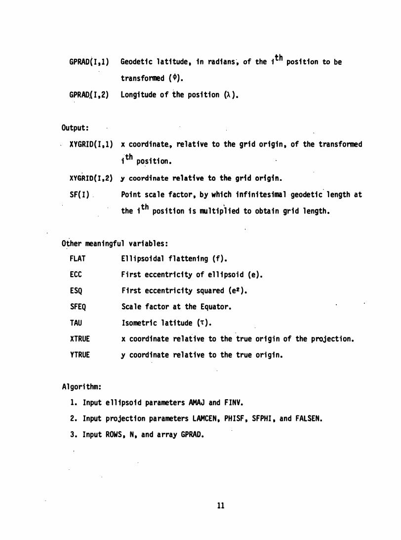
GPRAD{I,I ) Geodetic l atitude. in radians� of the ith position to be

transfonned (4)). GPRAD.(I ,2) Longitude of the posi tion (A ).

Output:

, XYGRID(I, l ) x coordinate" rel ative to the grid origin , of the transfonned

i"th pO,si ti on .

XYGRID(I,2) y coordinate relative to the grid origin. SF( I ) , Poi nt sca le factor , by which infi ni tesimal geodeti c l ength at

the i th posit10n i s multipl ied to obtai n gr1d l ength .

O�her meaningful vari abl es:

FLAT El lipsoidal fl attening (f) .

ECC First eccentricity of el l ipsoid (e ) .

ESQ First eccentricity squared (e2 ) .

SFEQ Sca le factor at the Equator.

TAU Isometr1c l atitude (T). XTRUE x coordinate rel ative to the true origin of the projection .

YTRUE y coordinate rel ative to the true origin .

Al gorithm:

1. Input e l l ipsoid parameters AMAJ and FINV.

2 . Input projection parameters LAMCEN, PHISF , SFPHI , and FALSEN.

3 . Input ROWS. N , and array GPRAD.

11

4. Compute el l ipsoidal constants ,

f = 1I( l/f)

e2 = f<.2 - f) e = Ce2)!.

5:. Compute the scal e factor a long the Equator,

" SFEQ = SFPHI ( cos �s)/ ( 1 - e2sin "2 �

s)i .

6. SAVE the constants ESQ", ECC , and SFEQ.

7 . Provi de" an alternate ENTRY poi nt named MERCF2 passi ng AMAJ , LAMCEN,

" FALSEN . ROWS , N . and GPRAD through the argument list.

S. I f no more forwa rd "-tran"sfonnati ons to perform, RETURN". Output gri d x· s , and y·s , �nd thei r respecti ve point scale factors.

9. For the next pai r of � and A in the i nput array, compute" the pl ane

" coordi nates rel ative to the true origi n ,

XTRUE = a A SFEQ

T ... In{�(1 + sin;\ ( 1 - e s�n4» eJ i} � 1 - s i �) 1 + e s1n,

YTRUE = a '\' SFEQ. ..

10. Compute the grid coordinates ,

IF C- 'IT � A - A 0 � 'IT ) XYGRID( I , I) II: XTRUE - aAoSFEQ

IF ( h - � > 'If" ) XYGRID(i ,1) = XTRUE - aCh o + 2rr )SFEQ

IF (- 'II" > h - hO> XYGRID( 1,1) = XTRUE - a ( AO - 2'IT)SFEQ

XYGRID(I,2) = YTRUE + FALSEN.

1 1 . Compute the point "scale factor,

SF ( I) II: SFEQ( l - e2sin� )!/co�.

12 . Repeat from step 8 for the next GP to be transformed.

12

References: 1 . Thomas , 1952 , pp. 85-86.

2 . Deetz and Adams . 1944 , pp. 1 12-115. ' 3. Snyder , 1983 , pp . 50-51.

Normal Mercator Inverse T�ansformlt1on (MERINY)

Input:

AMAJ FINV

LAMCEN

PHISF

SFPHI

FALSEN

ROWS

Sem1major axi s of elli psoid ( a ) .

Reciprocal of flattening (l/f) .

Central merid1,an of projection

, (�).

Absolute value of the geodetic latitude where scale factor ;s

known ( �s ) .

S�ale factor at PHISF.

False northi ng (yol.

Number of rows declared for the arrays GPRAD and XYGRID in the

calling program.

N Number of positions to be transformed.

XYGRID( I , I ) , x coordinate , relative to the grid origi n , of the i th position

to be transformed. '

XYGRID( I,2) Y coordinate relative to the grid origin.

13

Output:

GPRAD(I , I ) Geodeti"c l ati tude , i n radians , of the transfonned ith pos ition (<1». GPRAD(I ,2)

SF(I )

Longitude" of the pos ition (A ) .

Poi nt scale factor, by which i nfi ni tes imal geodeti c l ength at

the ith pos ition is m�lt ipl i�d to obtai n gri d l ength .

Other meani ngful variabl es :

FLAT El l ipsoidal fl attening (f) .

ECC Fi rst eccentri ci ty of el l i psoid (e ) .

ESQ Fi rst eccentricity "squared (e2 ) .

SFEQ Scale factor at the Equator.

YTRUE y coordi nate relative to the true origin .

Al gori thm:

-1. Input"ellipsoid parameters AMAJ and FINV.

:�2. Input projection parameters LAMCEN , PHISF , SFPHI , and FALSEN.

3. I nput ROWS , N , and array XYGRID.

4. Compute el l i psoidal constants ,

f ,= I/O/f) " e2 = f(2 - f)

e = eel)'" 5 . Compute the scale factor along the Equator .

SFEQ 1:1 SFPH I ( coScj)s )/O - e2si n2 <l>s )l.

6. SAVE the constants ESQ , ECC , and SFEQ.

7. Provide an al ternate ENTRY poi nt named MERCI2 , pass i ng AMAJ, LAMCEN ,

FALSEN . ROWS . N , and XYGRID through the argument l i st.

14

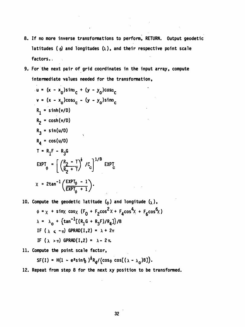
8. If no more inverse transformations to perform. RETURN. Output geodetic

latitudes (�) and longitudes (A ).t and their respective point scale

f�ctors .

9. For the next pai r of grid coordinates in the input array. compute the

y coordinate relat'1ve to the true origin .

YTRUE = y - Yo.

10. Compute an ini tial approximation of geodeti c l atitude (4) 1 ) '

t = lI{exp[YTRUE/ (aSFEQ)]} -

4> 1 = Tr /2 - 2tan-1 ( t) • . . 1 1 . Compute the next approximation of latitude (4)j+l' j = 1 ,2 .3 •••• ) .

' j+l = Tr/2 - 2tan-1{t[ ( 1 - e s in 4>j) / ( l + e S in4> j) ]e/2}.

12. Iterate step 11 unti l l4>j+l . 'j I < 5XI0·9rad•

13. Compute the l ongi tude .

� .= �o + x/[a(SFEQ)]

IF ( � '-'IT) GPRAD( I .2) = � + 2 Tr

IF ( �> Tr ) GPRAD( I .2 ) = �.;, 2Tr.

14. Compute the point s�ale factor.

SF ( I ) = SFEQ(1 - eZsinZ4» i/cos 4>. . .

15. Repeat from step 8 for the next xy position to be transformed.

Reference :

Snyder. 1983 . pp. 50-51.

15

. . Transverse Mercator Projection

The transverse Mercator projection i s often used where the area of i nterest l ies with .its l onger dimension in a north-south di rection . The true origin of thi s projecti�n i s at the intersection of the central meridian with the Equator. To maintain coordinates that are convenient for the area of interest . a .grid .origin may be establ i shed to the south and west of that area . A two-step procedure al l .ows definition · of the north-south l ocation of the grid origin in ei ther of two w�s: by speci fying a l atitude on whi ch the grid origin l ies or. by designating a val ue other than 0 for the y coordinate of the true origin. The two-step procedure involves transl ation of coordinates from the true origin .�o a fal se origin. then to the grid origin. . .

The fal se origin l ies on the central meridian of the projection and on the l at.itude of fal se origin. Y coordinates may be reduced · i n magnitude by . specifying a lat.i tude of fal se origin just to the south of the area of interest. If a false northing is specified rather than a latitude of false origin .• the false or1.gin 15 located at the intersection of the central meridian .with the Equator. - . - · The false northi ng. or grid y..�oordi nate of the fal se origi n ,· would be negative-valued in. the northern hemisphere , moving the .gri� origin northward. In the southern hemisphere the fal se northi ng would be positive-val ued . The fal se easting i s the x coordinate aSSigned to the fal se origin� It would be .positive in e1ther hemisphere.

Mapping equations . for the transverse . Mercator projection become unstable near the poles and 90°. off the central merid1an. From a practical standp01nt , use of the transverse · Mercator projection should be l imited to a region bounded by a maximum l atitude (±) and a l ongitudinal distance from the central meridian. The l imiting l atitude and l ongi·tudi nal distance wi l l depend on the purpose of the projecti on. .

Transverse Mercator Forward Transformition·(TMFWD)

Input:

AMAJ FINV

LAMCEN

FALSEE

FALSEN

PH I FAL

SFCEN

Semimajor axi s of el l �psoid (a) .

Reci procal of flattening (l/f) .

Central meridan of projection (Ao) .

Fal se easting (xo) . . . .

False northing (Yo) .

Geodetic l atitude of the fal se origin (.f) .

Scale facto� along central .meridian (ko) .

16

ROWS Number of rows declared for the arrays GPRAD and XYGRID i n the

cal l ing program.

N Number of positions to be transformed.

GPRAD(I.l) Geodetic latitude, in radians, of the ith

position to be

transformed (� ) .

GPRAD( I ,2 ) Longi tude of the position (A ) .

Output :

XYGRID( I , l ) x coordinate . relati ve to the grid ori gin , of the transformed

ith pos ition.

XYGRID( I ,2) y coordinate relative to the grid origin.

SF( I ) Point scale factor, by whi ch infi ni tesimal geodeti c l ength at

the i th position i s mul ti pl ied to obtain grid l ength.

Other meaningful va�iabl es :

FLAT El l ipsoidal fl attening ( f ) .

ESQ

E2SQ

ECC3

RN .

RREC

YVALUE

OMEGA

OMEGAF

S

ETASQ

First eccentricity of el l ipsoid , squared (eZ) .

Second eccentricity equared (eIZ) .

Third eccentri city ( n ) .

Radius of curvature in prime vertical .

Radius of recti fying sphere (r ) .

y val ue of true origin relative to fa l se origin .

Rectifying lati tude of the pOint in question (00). Recti fying latitude of fal se origin ( oof) .

Meridiona l distance .

Geodeti c variable ( nZ) representi ng the quanti ty eI2cosZ� .

17

XTRUE

YTRUE

XFALSE

YFALSE

x coordinate relative to the true origin of the projection .

y 'coordinate rel ative to the true origin.

x coordinate relative to the fal se origin.

y coordinate relative to the fal se origin .

Al gori thm:

1. Input el l ipsoi d parameters AMAJ and F INV.

2. Input projection parameters LAMCEN . FALSEE . FALSEN . PHIFAL . and SFCEN.

3. Inpu� ROWS . N . and array GPRAD. ,

4. Compute el l i psoidal constants , '

f = 1/(1/f)

e2 = f(2 - f)

e�2 = e2/ ( 1 - e2 )

n = f/(2 - f) .

5. Compute constants for meridional d1'stances .

� r = a( l - n ) ( l - n2) ( 1 + 9n2/4 + 225n4/64)

A2 = -3n/2 + 9n3/16

A4 = i5n2/16 - 15n4/32

� = -35n3/4S , As = 315n4/512

BO· 2(A2 - 2A4 + 3A6'· 4As)

B2 = S(A4 - 4A6 + lOAs)

B4 = 32(A6 • 6AS)

B6 = 12SAS•

6 . Detennine the y value of the true origin rel ative to the fal se origin,

Wf = �f + si�fco�f(Bo + B2cos24f + B4cos4�f + B6cos6�f)

YVALUE, = -kollJfr.

lS

7� SAVE the constants ESQ . E2SQ . RREC . YVALUE . 80, 82 , 84 , and 86•

8. Provide an al ternate ENTRY point named TMFWD2 , passing AMAJ. lAMCEN .

FALSEE , FALSEN , SFCEN , ROWS , N , and GPRAD through the argument l i st.

9. If no more forward transfonmati ons to perfonm , RETURN. Output grid XiS

and yls. and thei r·respective point scale factors .

10. For the next pai r of � and A in the input array , compute i ntenmediate

val ues needed for the transfonmation. Cos� and ta", should be assigned

to vari abl e names to avoid . repeated appl i cation of the i ntri nsi c cosine

and tangent functions . If � = ±n/2 . disabl e the tangent functioni the

tangent of � has no effect on the outcome i f � = ± V2.

n2 = el2cos� IF (- n �A-AO � n) L = (A - AO)COSet>

IF (A-\, > n) L =. (A- 1, - 2�cos�'

.

IF (-n > A-\') L = (A -AO + 2n) coset>

w = et> + s inet> coset>(BO + B2cos2et> + B4cos4et> + B6cos6et»

S = w r

RN � a/(1 - e2s i n2et»i

E3 = (1 - tan2et> + n2)/6

E4 = [5 - tan2et> + n2(9 + 4n 2 )]/12

E5 = [5 - 18tan2et> + tan4et> + n2(14 � 58tan2 et»]/120

E6 = [61 - 58tan2et> + tan4et> +n 2(270 - 330tan2et» ]/360

E7 = (61. - 479tan� .+ 179tan4et> - tan6 et»/5040

F2 = U'+n 2)/2 .

. F 4 =' [5 -' 4tan2et> + n 2(9 - 24tan� )]/12.

11. Compute the pl ane coor.dinates rel ati ve to the true origi n ,

XTRUE = ko(RN)L{l + L2[E3 + L2(E5 + E7L2 )]) YTRUE = .ko{S + RN(tanet» L2[1 + L2(E4 + E6L2)]/2) .

19

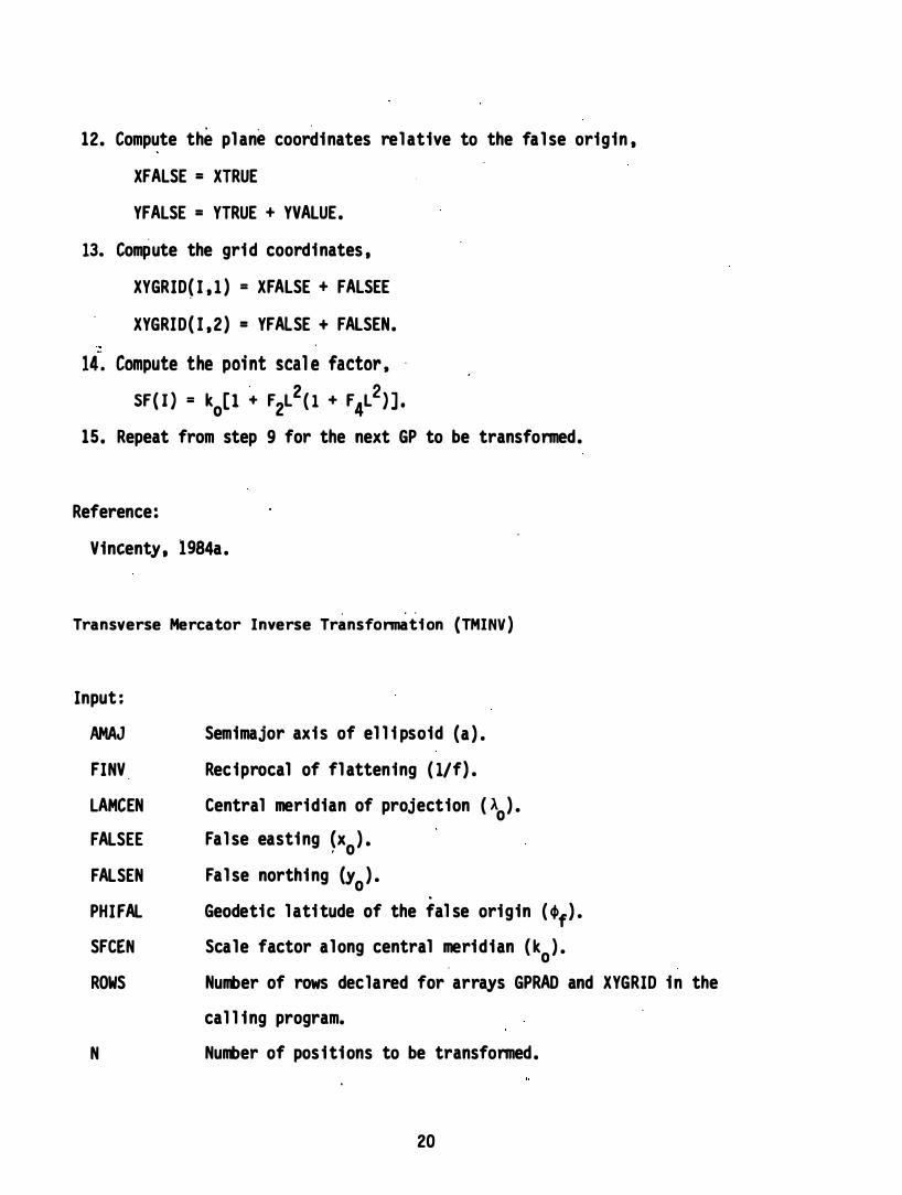
12. Compute the pl ane coordinates rel ative to the fa l se origin ,

XFALSE = XTRUE

YFALSE = YTRUE + YVALUE.

13. Compute the grid coordinates ,

XYGRID(I , l ) = XFALSE + FALSEE

XYGRID( I , 2 ) = YFALSE + FALSEN.

14� Compute the po;nt scale factor . .

SF(I) = ko[l � F2L2 ( 1 + F4L2)]. 15. Repeat from step 9 for the next GP to be transformed.

Reference:

Vincenty. 1984a .

. . . Transverse Mercator Inverse Transformati on (TMINV )

Input:

AMAJ Semimajor axi s of el l i psoid (a ) .

FINV Reciprocal of fl attening ( l/f) .

LAMCEN

FALSEE

FALSEN

PHIFAL

SFCEN

ROWS

N

Central meridian of projection ( Ao) '

Fal se easting �xo ) '

Fal se northing (Yo ) ' .

Geodetic l ati tude of the false origin ( 'f) '

Scale factor along central meridian ( ko ) ' . .

Number of rows declared for arrays GPRAD and XYGRID in the

cal l ing program.

Number of pos itions to be transformed.

20

XYGRID( I ,I ) x coordinate, relati�e to the grid ortgin , of the tth positton

to be transfo�d. . .

XYGRID(I,2) y coordinate relative to the grid origin.

Output: .

GPRAD(I,l) Geodetic l atitude , in radians , �f the transformed ith posi tion(.).

GPRAD(I.2) Longitude of the position (�).

SF( I ) Point scale factor, by which infinttestmal geodetic l ength at

the tth positton is mul tiplted to obtain grid l ength.

Other meaningful variables:

FLAT El l ipsotdal fl attening (f).

ESQ Fi rst eccentricity of el l ipsoid , squ�red (e2).

E2SQ Second eccentrictty squared (eI2 ).

ECC3 Thi rd eccentrtctty (n).

RNFP Radius of curvature tn prtme vertical . at the footpoi nt

latitude.

RREC

YVALl/E

OMEGA

OMEGAF

LATFP

S

ETASQ

Radi us of recttfying sphere ( r).

y val ue of true .origin �l�t;ye to fal se origin.

Rectifying l atitude of the point in question �). Rectifying l atitude of .fal se origin (wf).

Footpoint l atttude ( �p).

Meridional distance.

Geodetic variable (n2 ) representing eI2cos2�.

21

Al gorithm:

1 . Input elli psoid parameters 'AMAJ and F INV.

2. Input pr.ojection parameters LAMCEN . FALSEE . , FALSEN . PHIFAL . and SFCEN.

3. Input ROWS . N. and array XYGRIO.

4. Compute el l ipsoidal constants . '

f = I/O/f) ,

e2 = f(2 • f)

n = f/(2 - f)�

5. Compute constants for meridional distances .

r = a ( 1 - n ) ( 1 - n2) ( 1 + 9n2/4 + 225n4/64)

A2 = -3n/2 + 9n3/16

A4 = 15n2/16 - 15n4/32

A6' = -35n3/48 As = 315n4/512

BO = 2 (A2 - 2A4 + 3A6 - 4Aa)

82 = 8 (A4 - 4A6 + I°As)

B4 = 32(A6 - 6Aa) ,

B6 = 12SAa

C2 = 3"/2 - 27n3/32

C4 = 21n2/16 - 55n4/32

C6 = 151n3/96

Cs = 1097n4/512

DO = 2(C2 - 2C4 + 3C6 - 4CS)

D2 = 8(C4 - 4C6 + 10Cs)

04 = 32(C6 -.6CS)

D6 = 12SCS•

22

6. Detenmine the y value of the tru e ori gin rel ative to the false or;gin. 2 4 6 W, = 4>f + s inj>fcoScjlf(BO + B2cos <If + B4cos 4>f + B6cOS <l>f)

�VALUE = -kowfr. 7. SAVE the constants ESQ . E2SQ , RREC, YVALUE . DO, O2, 04, and 06" 8. Provi de an alternate ENTRY poi nt named TMINV2, passing AMAJ, LAMCEN,

FALSEEi FALSEN . SFCEN , ROWS . N , and XYGRID through the argument li st .

9. If no more inverse transformations to perform. RETURN. Output geodetic

lati tudes (�) and longi tudes (A). and thei r respective point scale

factors . 10. For the next pai r of grid coordi nates in the input array , compute

i ntermediate values needed for the transformation . Cosw and tan<l>fp shou l d be assigned to vari able names to avoid repeated appl icati on of the i ntrinsic cosi ne and tangent functions . If w = ±n/2, computation of the remaining i ntermediate values i n thi s step are ski pped; in step 1 1 . <I> = w, A i s i ndeterminate and may be set equa l to Ao for convenience; and in step 12, the point sca le factor equa l s ko•

w = (y - Yo - YVALUE)/ (kor) <l>fp = w+ s i n w CO5(£) (Do + D2cos

2w + D4COS� + D6cOS�W) RNFP = a/O - e2s in2 clfp )i

2 = e.2cos2 dl.. nfp �p 2 G2 = -tan <l>fp( l + nfp )/2

2 2 G3 = -0 + 2tan <l>fP + nfp )/6 G4 = -[5 + 3tan2<1>fp + n,p

2( 1 - 9tan2<1>fp ) - 4nfp4J/12

G5 = [5 + 28tan2<1>fp + 24tan4<1>fp + nfp2 (6 + 8ta�2 <1>fP )]/120

G6 = [61 + 90tan2<1>fp + 45tan4<1>fp + nfp2(46 - 252tan2<1>fP

- 90tan4<1>fP) ]/360

23

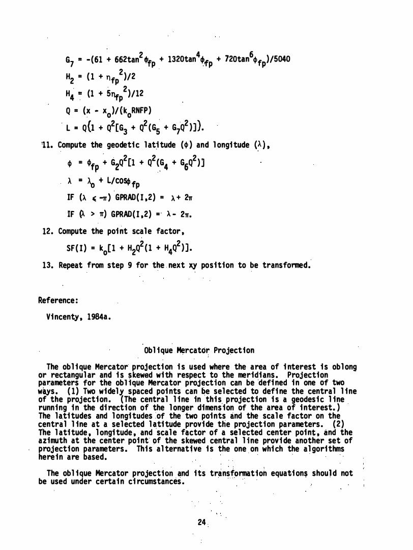
G7 = - (61 + 662tan2'fp + 1320tan4�fP + 720tan6�fP )/5040 2 .

H2 = ( 1 + nfp )/2 H4 � (1 + 5n,p

2)/12

Q = (� - xo)/{koRNFP ) . L = Qb + Q2[G3 + Q2 (G� + G7

·Q2 )]). 111. Compute the geodetic lat�tude (� ) and longitude (�),

. · 2 2 2 . tP = tPfP

+ G2Q [1 + Q (,G4 + G6Q )]

A = Aa + L/ COScfl fp IF (A '""'IT) GPRAD(I,2) = A + 2'1f IF (A > 'If) GPRAD(I,2) =. A - 2'1f .

12. Compute the poi nt scale factor,

SF(I) = ko[1 + H2Q2 ( 1 + H4Q

2 )] .

13. Repeat from step 9 for the . next � position to be transformed.

Reference : Vincenty, 1984a .

Oblique Mercator Proj�ction The oblique Mercator· projecti on i s used where the area of i nterest i s oblong

or rectangular and i s skewed wi th respect to the meridians . Projection . parameters for the ob1 1que Mercator projection can be ·defi ned i n one of two ways . ( 1 ) Two widely spaced poi nts can �e selected to defi ne the central line of the projection. (The central line in thi s projection i s a geodesic line running i n the di rection of the longer dimens·ion of the area of i nterest. ) . The la.titudes and longitudes :of the two points and the scale factor on the central line at a selected l�titude provide the projection parameters. ( 2 ) The lati tude, longitude, and scale f�ctor of a selected center point, and the azimuth at the center poi nt· �f the skewed central line provide another set of projection parameters . Thi s alternative i s the one . on which the algorithms herein are based. . .

The oblique Mercator project10� and its transf�rmatioh equati on$ should not be used under certai n ci rcumstances. . . . . .. . .

24 .

1. If the center poi nt of the area of i nterest lies near ei ther pole. use the stereograph;c projection i nstead ( not included in this report). .

2. If one of the two widely spaced poi nts defi ning the projection lies at either pole. u se equations for the transverse Mercator projection i nstead.

3. If the two widely spaced poi nts both lie on the Equator , use equations for the nonmal Mercator projection i nstead .

4. In general , if the two widely spaced pOi nts lie on the same paral l el Of lati tude other than the' Equator. use equations for the Lambert conformal conic projection i nstead. Note , however, that if the parallel of latitude on which the two defin ing poi nts lie i s close to the Equator, a normal Mercator projection may be used .

The true orig in of the projection lies at the i ntersection of the central line with the Equator of the so-called aposhere (Hotin e 1946-47). such point bei ng near the true Equator of the Earth. For Alaska zone 1 (SE Alaska) the true origin i s i n the vici nity of 00 lati tude . -1010 l ong itude . The gri d ori gin lies at a speci fied poi nt .near the area of i nterest, south and west of the center poi nt . For Alaska zone 1 , that poi nt i s 5.000 ,000 meters to the north and 5,000 ,000 meters to the west of the true origi n .

The algorithms for transformation of coordinates are based on Hotine's " recti fied skew orthomorphi c" projection . Equations were obta ined from T. Vi ncenty ( 19S4b ) of NGS and were further manipulated to el iminate application of the natural logari thm when the exponential function woul d subsequently be applied.

Obl ique Mercator Forward Transformation (OMFWD)

Input: AMAJ FINV PHICEN

. " LAMCEN SFCEN AZICEN

FALSEN FALSEE

Semimajor axi s of ellipsoid (a) . Reciprocal of flattening ( lIf) . .

Geodetic latitude of the center poi nt of the projection (�c ) . Geodetic' longi tude of the center point (Ac ) •

Scale factor at the center poi nt (kc ) . Geodetic azimuth at the center poi nt of the skewed center line (ac ) . False northi ng (Yo) . False 'easting (xo ).

25

ROWS Number of rows declared for array GPRAD and XYGRID in the

cal l i ng program.

N Number of pos.i ti on·s to be transformed.

GPRAD( I , l ) Geodeti c l ati tude, i n radians, of the i th pos ition to be

transformed (cjl ) .

"GPRAD( I,2 ) Longi tude of the ' posi tion u ) .

Output: . ,

XYGRIDO . l ) x coordinate . relati"ve to the gri d ori gi n , of the transformed ith position.

'XYGRID( I ,2 ) y coordinate rel ative to the grid ori gin . 'SF( I ) Poi nt · sca le factor, by whi ch i nfi ni tesimal geodeti c l ength at

the ith position is mul ti pl ied to obta in grid l ength .

Other meani ngfu l variabl es :

'FLAT El l i psoidal fl atteni ng (f ) . ECC Fi rst eccentric ity of el l ipsoi d (e ) . ESQ. Fi rst eccentricity squared (e2 ) . E2SQ Second eccentricity squared · ( e ' 2 ) . WSQ Geodeti c vari able (WI ) representi ng the qual i ty 1 - e2si n2cjl . EXPT Natural base of l ogari thms rai sed to the T power. where T (T)

i s the i sometri c l atitude. LAMO .

USKEW Geodetic l ongi tude of the true orig in (Ao ) . u coordinate i n the recti l i near coordinate system wi th the ori gin at the center poi nt and u axis a l ong the projected skewed center l ine.

VSKEW 'v 'toordinate i n the skewed recti l inear coordinate system.

26

Algori thm: 1 . Input elli psoid parameters AMAJ and FINV.

2. Input projection parameters PHICEN , LAMtEN , SFCEN , AZleEN , FALSEN , and

FALSEE.

, 3. Input ROWS , N , and arr� GPRAD. 4. Compute elli psoidal constants ,

f = I/O/f) e2 = f(2 - f) e = (e2 )t

e l 2 = e2/ ( 1 - e2 ) . S . Compute zone constants .

W 2 = 1 _ e2si n2� c c B = ( 1 + e , 2cos4�c)i

A =' B( l _ e2 )t/W 2 c E,XPT = [G + s i ncjlc\ (1 - e s �ncjlc\ eJ i

c 1 - s 1�c) 1 + e S l��) 1

Sc = WcA/cos�c C = S + ( S 2 - l )t c c c Jc = ( Cc - �/Cc)/2 o = kc(A/B )a F = s 1nao = s inaccos�c/ (WcA) G = cosao = cOS (S in-1F) A = A - s 1n- 1 (J F/G)/B o c c H = kcA.

6. SAVE the constants ESQ . ECC . B, EXPTc ' Cc ' 0, F, G. LAMO . and H.

27

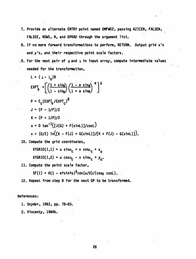
7 . Provide an al ternate ENTRY point named OMFW02 , pass ing AZ leEN , FALSEN , FALSEE . ROWS . N . and GPRAO through the argument l i st.

8. If no more forwar� transformations to perform, RETURN. Output grid X i S and y l s , and . thei r respecti ve poi nt sca le factors .

:.9 . For the next pa i r of ct> and A i n i nput array . compute i ntennediate val ues needed for the transformation ,

L = ( A - \,)8

EXPT = [(1 + sitlb\ (1 - e S inw\ e ] i if> 1 - Si"ct» 1 + e s i�)

P = Cc ( EXPTcjI /EXPTc)8

J = (P - l/P )/Z K = (P + 1/P)/2 u = 0 tan-1([J (G) + F (Si nL ) ]/coSL)

v = (0/2 ) I n([K - F(J ) + · G( s inL) ]/[K + F(J ) - G(s inL ) ]}. 10 . Compute the grid coordi nates ,

XYGRIO( I . l ) = u s i nac + v C05ac + Xo XYGRIO( I ,2 ) = u cosac - v s i nac + Yo .

1 1 . Compute the point scale factor , SF( I ) = H ( l. - e2si ri2tj» icos (u/0}/ (coScf> cosL ) .

12 . Repeat from step 8 for the next GP to be transformed.

References : 1 . Snyder , 1983 , pp . 78-83.

2 . Vi ncenty , 1984b .

28

Obl ique Mercator Inverse Transformation (OMINV )

Input: AMAJ FINV

PHICEN

LAMCEN SFCEN AlICEN

FALSEN FALSEE ROWS

N

Semimajor axi s of el l i psoi d (a) .

Reci procal of fl atteni ng ( I/f) • .

Geodet1c l at1tude of the center poi nt of the projecti on (�c ) • .

Geodetic l ongitude of the center poi nt (Ac ) . Scale factor at the center poi nt (kc ) . Geodetic azimuth at the center poi nt of the skewed center l ine (ac ) . Fal se northi ng (Yo ) . Fal se easting (xo ) . Number of rows ·declared for arrays . GPRAD and XYGRID 1 n the ca 1 1 1 ng program. Number of posi tions to be transformed.

XYGRID(I . I ) x coordinate . relative to the grid ori gi n . of the ith posi tion to be transformed.

XYGRID(I .2) y coordinate relative to the grid ori gin .

Outpait : . GPRAD(I . l ) GPRAD(I .2 ) SF( l)

Geodeti c latitude . in radians , ·of the transformed ith pos i tion (� ).

Long.i tude of the position (A ) . Point scale factor , by which i nfi ni tesimal geodetic l ength at the i th posi tion i s mul tipl ied to obtain grid l ength .

29

Other meani ngful variables : FLAT Elli psoi dal flatteni ng (f) .

ECC

ESQ

E2SQ

�WSQ ;..EXPT

LAMO

CHI USKEW

Fi rst eccentric1 -ty of elli psoid (e) . ,

Fi rst eccentricity squared (el ) . Second eccentricity squared (e l l ) .

Geodetic variable (W2 ) representing the quanity 1 - e2sin2,.

Natural base of logarithms rai sed to the, T power, where T (or ) i s the 'i sometri c latitude . Geodetic longitude of the true origin . (Ao ) . Conformal lati tude of the point 1 n question (X ) . u coordinate i n the rectilinear coordinate system with the

origin at the center poi nt and u axis along the projected ,

skewed center l ine.

VSKEW v coordinate i n ,the , skewed rect1linear coordinate system.

Algori thm: 1 . Input ellipsoid parameters AMAJ and FINV.

2. Input projection parameters PHICEN , LAMCEN . SFCEN . AZICEN , FAL5EN , and FALSEE.

3. Input ROWS . N. and a rray XYGRID.

4 . Compute el l ipsoidal constants ,

f = I/ O/f)

e2 = f(2 - f)

e = '(e2 ).

e l 2 = e2/ ( 1 - el ) .

30

5 . Compute zone constants . W 2 = 1 - e2s i n2 cfl c c B. = ( 1 + e l 2cos4 cfl )1 c A = B ( I _ e2 )1/w 2 c

EXPT '= [(I + S i n�c)(1 ". e Sincp� eJ i

c 1 - s i n�c

1 + e Sin�� Sc = WcA/co� c ' C = S + ( S 2 _ I)i c c c Jc = (Cc - I/Cc )/2 o = kc (A/B )a F = s inao = s i naccoS�c/ (WcA) G = C0910 = COs (s i�-IF)

10 = 1c - s i n-1 (JcF/G)/B H = k A c C2 = e

2/2 + 5e4/24 + e6/12 + 13eS/360 C4 = 7e4/4S + 2ge6/240 + SIleS/11520 C6 = 7e6/120 + SleS/ 1120 Cs = 427geS/ 1612S0 FO = 2 ( C2 - 2C4 " + 3C6 - 4Cs) F2 = S(C4 - 4C6 + IOCS) F4 = 32(C6 - 6CS) F6 = 12SCS•

6 . SAVE the constants ESQ . B . EXPTc ' Cc ' D . F . G . LAMO, H , FO� F2 , F4 and F6 7 . Provide an a l ternate ENTRY point named OMINV2 , passing AZICEN . FALSEN ,

FALSEE , ROWS , N . and XYGRID through the argument l i st.

31

8. If no more i nverse transformations to perform, RETURN. Output geodetic l ati tudes ( cp) and l ongi tudes (A ) , and thei r respecti ve poi nt sca le factors • .

9., For ' the next pai r of grid cOO,rdi nates i n the i nput array , compute

i ntermedi ate 'val ues needed for the transformation ,

' u = (x - Xo )S iRlc + (y - yo )casac v = (x - xo )cosac - (y - Yo) slnac R1 = s inh (v/D) R2 = cosh (v/D) R3 = s i n (u/D)

R4, = cos (l(/D) T = RIF - R3G )i ] l/B EXPT = [ (R2 - T Ie ' EXPT cp R + T e e 2 ' X = 2tan-1 ( EXPTcp - 1) .

EXPTcp + 1

10. Compute the geodetic l atitude (cp ) and l ongi tude (A ) ' cp = X + s i nx COSX ( FO + F2cos

2x + F4cos� + F6cos� ) A = AO + {tan-1[ ( R1G + R3F)/R4J) /B IF ( A , - 1T) GPRAD( I , 2 ) = A + 21T IF ( A > 1T) GPRAD ( I ,2 ) = A - 2 1T.

1 1 . Compute the poi nt. sca le factor, SF ( I ) = H(1 .. e2s in\ )iR4/{coscp COS[ ( A - Ao )BJ} .

12. Repeat from step 8 for the next xy posi tion to be transformed.

32

References : 1 . Snyder , 1983 , pp . 83-84. 2 . Vincenty , 1984b .

Lambert Conformal Conic Projection

The Lambert conformal conic projection i s often used where the area of i nterest l ies with i ts l onger dimension i n an east-west d irection . The fundamental projection parameters are centra l mer;d;an " central paral l el , and mapping rad1us of the Equator. Usual ly , north and south standard pa ra l l e l s are speci fied rather than a central paral l el , whi ch does not l ie exactly hal fway between the standard paral l el s . The next al gori thm requ i res i nput of north and south paral le l s ( not necessari ly standard) , and scal e factor at the centra l paral l el ( not necessari ly known ) . It handl es three cases for defin ing the projection . '

Case 1 - Secant projection wi th north and south standard paral l el s known : i nput a central sca le factor of 0 , and the north and south standard paral l el s .

Case 2 - Secant projection wi th central para l lel and i ts scale factor known : i nput the known central sca le factor, and north and south paral lel s equal to the central paral lel .

Case 3 -, Tangent projection : i nput the central sca l e factor of 1 (exactly ) , and north and south paral l el s equal to the central paral l el .

The true ori gin of the Lambert co�formal conic projection i s at the i ntersection of the central meridian wi th the apex of the cone on which the projection i s made . Thus , true y coordi nates are al l negati ve for projecti ons in the northern hemi sphere , and are a l l positive for projections in the southern hemi sphere . To mainta in positive-val ued y coordi nates i n an area that was of i nterest when a particul ar zone was fi rst defi ned , a latitude of fa l se orig in may have been speci fi,ed to the south of the central paral l el . The i ntersection of the central meridian wi th the l ati tude of fal se orig in gives the fa l se orig in . Subsequent to the ori ginal defi ni tion of zone , a fa l se northi ng may have been assi gned to the fal se origin al l owing the zone to be extended farther south without encountering negative coordinates . Appl ication of the fal se northi ng and the fal se easti ng to the fal se origin provides the gri d ori gi n . The 'fol l owing a l gori thms are val id i n ei ther hemi sphere when the conventional meanings of north and south are mai ntai ned i n the above di scussion .

33

Lambert Conformal Conic Forward Transformation (LCCFWD )

Input: AMAJ FINV

-LAMCEN

PHIN

PHIS SFN PHIFAL FALSEN FALSEE ROWS

Semimajor axi s of el l i psoid ( a ) .

Reciprocal of · .fl attening ( l/f) .

. Central meridan of the projection (Ao)

North para l l e� (:�n ) . South paral l el ( �s ) . Scale factor along the north (or south ) paral lel ( kn ) . Geodetic l atitude of fal se origin ( �f) . -Northi ng val ue , usual ly 0, speci fied for the fal se . origin (Yf) . Fal se easting (xo ) .

Number of rows declared for arrays GPRAD and XYGRID i n the

cal l fng program. . .

N Number of ' pos iti ons to 'be transformed.

GPRAD( I , l ) Geodetic l atitude . i n radians . of the ith pos ition to be transformed (IP ) .

GPRAD( I ,2 ) Longitude of the posi tion (A ) .

Output:

XVGRID( I , l ) x coordinate ; rel ative to the grid orgin . of the transformed i th pos i tion .

XVGRID( I , 2 ) y coordi nate relative to the grid origin . SF( ! ) Poi nt s.cal e factor. by whi ch i nfi ni tesimal geodetic l ength

at the ith position i s mul ti pl ied to obtai n grid l ength .

34

Other meaningful variables :

FLAT ECC ESQ

PHICEN

EXPT

RAD

RADEQ RADFAL THETA

Ellipsoidal flatteni ng (f) . Fi rst eccentrici ty of ellipsoid (e) . Fi rst eccentricity squared (e2 ) . Central parallel (�o) .

Natural base of logarithms rai sed to the T power, where T (t ) i s i sometric latitude . Mapping radius.

Mapping radi us at Equator. Mappi ng radius at latitude of false ori gi n . Mapping angle (9 ) .

Subscri pts ri , s , o . and f denote quanti ties associated wi th �n ' �s ' �o ' and �f' respecti vely.

Algorithm: 1 . Input elli psoid parameters AMAJ and FINV.

2. Input projection parameters LAMCEN . PHIN , PHIS . SFN , PHIFAL , FALSEN , and FALSEE.

3. Input ROWS . N . and array GPRAD. 4. For computation of zone constants , repeated computation of EXPT and of W

merit functi on subprograms ,

EXPTAU(cf» = [(1 + si n�) (1 - e slncf>\ eJ i 1 - s in� 1 + e s i ncf»

W(cf» .. ( 1 - e2sin'cf» ' .

35

5" Compute e 1 H ps01 da 1 constants . f = l/ ( l/f) e2 = f( 2 - f) e = (e2 )i .

6 . Compute zone constants .

IF (�n = �s ) THEN

�o = �n " RADEQ = k a EXPT s 1n�o/ (W tan � ) n 0 0 0

IF ( �d � �s ) THEN

s 1ndl = I n[Wncos�sl(WscoS;n )] o I n(EXPTn/EXPTs)

RADEQ " = kn a COS�n( EXPTnS 1n�0 )/ (WnS 1n�0 ) .

RADFAL = RADEQ/ ( EXPTfs1 n �0 ) .

7 . SAVE the constants ECC . ESQ . RADEQ . s 1n�0 ' and RADFAL • . � 8. Prov ide an al ternate ENTRY poi nt name� LCCFD2 . passing AMAJ , LAMCEN ,

FALSEN , FALSEE , ROWS , N , and GPRAD through the argument l i st . 9. If no more forward transformat10ns to perform. RETURN. Output grid X i S

and y l s and "thei r respect1 ve p01 nt sca le factors . 10. For the next pa1 r of � and A 1 n the 1 nputl arr� , compute 1 ntermediate

val ues needed for the transformation , RAD = RADEQ/ ( EXPT s 1ncj)o ) " e = (A - Ao ) s i n4>o .

1 1 . Compute the grid coord1nates , XYGRID( I , l ) = Xo + RADsl ne XYGRID ( I ,2 ) = RADFAL + Yf - RADcos e.

36

12 . Compute the poi nt sca le factor ,

SF( I ) = W� {RADsin�o )/(a co� ) .

13. Repeat from step 9 for the next GP to be transformed.

Reference : Vincenty , 1985.

Lambert Conformal Conic I nverse Transformation (LCCINV)

Input : AMAJ

FINV LAMCEN PH IN PHIS SFN PHI FAL FALSEN FALSEE ROWS

N

Semimajor axi s of el l i psoid (a ) .

Reci p�ocal of fl atteni ng ( l/f) . Central meridian of projection ( Ao ) . North paral l el (�n ) . · South paral lel (�s ) . Sca le factor along the north ( or south ) paral lel ( kn ) . Geodetic l atitude ' of fal se orig in (�f) . Northi ng val ue , usua l ly 0 , speci fied for the fal se origi n (Yf) . Fa l se east1ng (xo ) . Number of rows dec lared for arrays GPRAD and XVGRID i n the cal l i ng program. Number of positions to be transformed.

XYGRID ( I , l ) x coordinate , rel ati ve to the grid ori gi n , of the i th pos i ti on to be transformed .

XYGRID{ I ,2 ) Y coordinate relati ve to the gri d ori gi n .

37

Output : GPRAD( I , l ) GPRAD( I , 2 ) SF( I )

Geodetic l atitude , i n radians , of the transformed i th position (� ). Longitude of the posi tion (:\ ) . Point sca le factor, by which infinitesimal geodetic length at the ith pos ition i s mul tipl ied' to obtain grid l ength .

Other meaningful variables :

FLAT

ECC

ESQ

PHICEN

TAU EXPT

. . w

RAD RADEQ RADFAl

XTRUE YPRIME

El l i psoidal fl attening (f) .

Fi rst eccentrici ty of el l i psoid (e) .

Fi rst eccentri ci ty squared (e2 ) .

Central paral lel ( �o ) . Isometric l atitude (T ) . Natural base of l ogarithms raised to the T power, where T (T ) i s the i sometric l ati tude. Geodetic variable ·representing the quanti ty ( 1 - e2sin� )i •

Mapping radius . Mapping radius at Equator. Mapping radius at l atitude of fal se origin.

x coordinate rel ative to the true origin . Di stance a long central meridian from apex of projection to y coordinate of the point in question .

THETA Mappi ng angle (e ) . Subscripts n , s , 0 , and f .denote quantities associated wi th �n ' � s . �o ' and �f ' repectively.

38

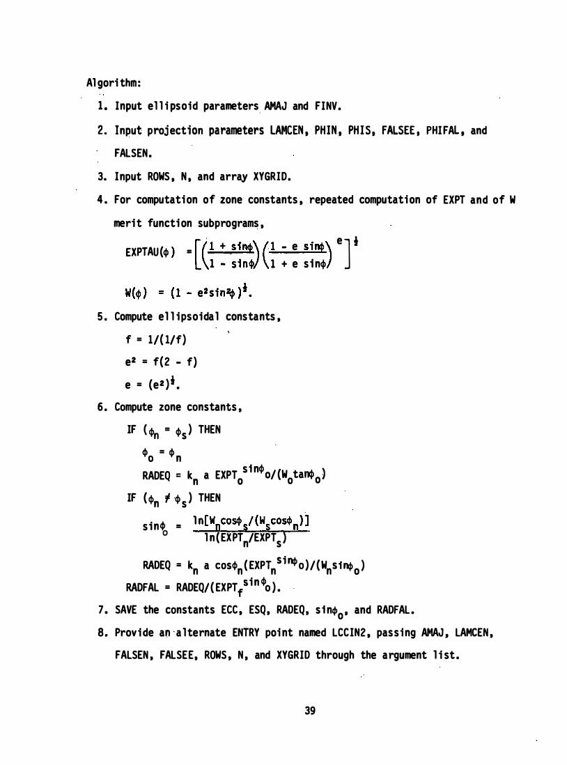
Al gori thm: 1 . Input el l i psoid parameters. AMAJ and FINV.

2 . Input projection parameters LAMCEN , PHIN , PH IS , FALSEE , PHIFAL . and FALSEN.

3. Input ROWS , N , and array XYGRID. 4. For computation of zone constants , repeated computation of EXPT and of W

merit function subprograms , . e i

EXPTAU(<I» = [(1 + .s i ne/!\ (1 - e S i�) ] 1 - s 1 n<l>J 1 + e s 1 n<l>

5 . Compute el l i psoida l constants , f = 1/( I/f) e2 = f(2 - f) e = (e2 )i .

6 . Compute zone constants , IF ( <I>n = <l>s ) THEN

<1>0 = <l> n RADEQ = kn a EXPTo

s1 n<l>o/ (WotanPo) IF (<I>n � ·<I> s ) THEN

s in� = 1 n[WncoS<!>s/ (WsCOS<l>n ) ] o I n ( EXPTn/EXPTs )

RADEQ = kn a COS<l>n ( EXPTnSl�o)/(WnSf�o )

RADFAL = RADEQ/( EXPT/ i n cllo ) . .

7 . SAVE the constants ECC , ESQ, RADEQ, s 1 n<l>o ' and RADFAL . 8. Provide an · a l ternate ENTRY poi nt named LCCIN2 , pass ing AMAJ , LAMCEN ,

FALSEN , FALSEE, ROWS , N , and XYGRID through the argument l i st .

39

9. ' If no more forward transfonnations to perfonn. RETURN. Output geodetic l ati tudes (� ) and l ongi tudes ( A) � and the ir respective poi nt sca le factors .

10. For the next pai r of grid coordi nates ,i n the i nput arr�. compute intermediate val ues needed for the transfonnation .

XTRUE = x - x ' o YPRIME = RADFAL + Yf - Y e = tan-1 ( XTRUE/YPRIME) RAD = (XTRUE2 + YPRIME2 ).

EXPT� = I RAOEQ/RAOI ( l/s �n�o) . 11 . Compute an in itial approximation of the s i ne of the geodetic

'., l atitude . g ivi ng it the a l gebrai c s ign of cfl o ' , si n cfl1 = ( EXP\ 2 - 1 )/ ( EXPTcfl

2 + 1 ) . '

12'. Iterate for S incflj+l three timl!s '(j = I �2 .3 ) as fol loWs : F1 = I n ( EXPTcflj IEXPT� ) F2 = 1/ ( 1 - s in2cfl · ) - e2/ ( 1 - e2s in2cfl · )

' J , J si n cl>j+l = s i ncl>j - F1/F2 .

13. Compute the geodeti c l atitude (cfl )- and l ongi tude (A ) . cfl = s i n-1 ( s incl>4)

, A = A 0 + e Is i ncpo IF ( A ' -'1'1') GPRAD( I .2 ) = A + 2IT I F ( A > 1T ) GPRAD( I . 2 ) = A,- 2 'IT.

14. Compute the point sca le factor . SF( I ) = ( I, - e2si n2�4) iRADs i ncl>o/ (a cos�4) .

15 . Repeat from step 9 for the next � pos it ion to be transformed.

40

Reference : Vincenty. 1985.

Polyconic Projection

There are $everal different polyconic projections . Each has a central meridian represented by a strai ght l ine and paral lel s of l atitude, representl by nonconcentric arcs of c1 rcles , the centers of. whi ch fal l on the extens10 of the central meridian. In thi s report , the term "polycon1c" refers to th ordinary (or American ) polyconic projection . Thi s projection has appl i cati l in cartography . but not in surveyi ng.

Scale along the central meridian is constant and equal to sca le along al l paral lel s of l ati tude . El sewhere . sca le varies with direction . The ordina polyconic projection i s not conformal . so poi nt scale factors are not determined in the fol lowing al gori thms .

The true ori gin of the polycon1c projection l ies at the i ntersection of t, central meridian with the Equator. True pl anar coordinates are reckoned f� the true orig in . Grid coordinates are reckoned from a grid origi n , which i defi ned by a specified l atitude and a fa l se easting . The al gorithm for the i nverse transformat10n (and the projection i tsel f for that matter) must not used at l ongitudes greater than 90° from the central meridian .

Polyconic Forward Transformation (PCFWD)

Input : AMAJ FINV LAMCEN FALSEE PHIG SFCEN

Semimajor axi s of el l i psoid (a ) . ,

Reciprocal of flatteni ng ( l/f) . Central meridian of projection bol e Fal se easti ng (xo ) . Geodetic l atitude of the grid 'origin (� g ) . Scal e factor a long the central meridian ( for the case at hand , a cartographic scale factor) ( ko ) .

ROWS Number of rows declared for arr�s GPRAD and XYGRID i n the cal l i ng program.

41

N Number of pos itions to be transformed .

GPRAD( I , l ) . Geodeti c l atitude , i n "radians , of the i th pos i t i on to be

trans�onned <4» .

GPRAD( I , 2 ) . Longi tude of the pos i ti on (l ) .

Output:

�kVGRID( I , l ) x coord i nate , relati ve to the grid ori gi n , of the transformed

i th pos i ti on .

XYGRID ( I ,2) y coordi nate rel at i ve to the gri d ori g i n .

Other mean i ngful variables :

FLAT

ESQ

ECC3

RN

RREC

OMEGA

OMEGAG

YVALUE

S

THETA

• XTRUE

YTRUE

El l i posoldal fl atteni ng ( f ) .

Fi rst eccentri ci ty of el l i pso,d . squared" (eZ ) .

Th i rd eccentri city ( n ) .

Radius of curvatu re i n the prime vert i cal .

Radi us of rectifying sphere ( r ) . .

Recti fyfng l atitude of the poi nt i n question (00 ) .

Recti fyi ng l a t i tude of grid ori g i n (OOg) . "

y val ue of true orl g i n rel ati ve to gri d ori g i n "(Yo ) .

Meri diona l di stance .

Mapping angle <e ) .

x coord i nate rel ative to the true ori g i n of the projection .

y coordi nate rel ati ve to the true ori g i n .

42

Algori thm:

1. Input el � ipsoi dal parameters AMAJ and FINV .

2. "Input projection parameters LANCEN, FALSEE , PHIG , and SFCEN.

3. Input ROWS , N , and array GPRAD.

"4. Compute el l ipsoidal constants ,

f = l/(1/f)

e2 = f{2 - f)

n II f/(2 - f) .

5. Compute constants for meridional distances ,

r = a(1 - n )(1 - n2)(1 + 9n2/4 + 225n4/64)

A2 = -3n/2 + 9n3/16

A4 = iSn2/16 - ISn4/32

� • -35n3/48

As = 31Sn4/512

BO = 2(A2 - 2A4 + 3A6 - 4Aa) 82 II 8(A4 - 4� + lOAa)

84 = . 32(A6 - 6Aa)

B6 • 128Aa·

6. Detenn1ne the y val ue of ihe true origin relative to the grid ortgtn

(whi ch is the meridional distance to the grtd origin ) ,

IF ( .g II 0) YVALUE = 0 IF (41g � 0) THEN

�g • � + S1�.gCO�g(Bo + B2cos2•g + B4cos4•g + B6cos6 •g )

YVALUE • -ko�gr.

7. SAVE the constants ESQ. RREC, ·YVALUE. BO' B2 • B4, and B6-

43

8. Provide an al ternate ENTRY poi nt named PCFWD2 , passing AMAJ , LAMCEN ,

FALSEE, SFCEN , ROWS , N , and GPRAD through the argument l i st.

9. If no more forward transformations to perform, RETURN. Output grid XiS

and y l s .

to. For the next pai r of � and A i n the i nput array , compute i ntermedi ate

. . , val ues needed for the transformation ,

e == ( A- \, )s;n�

w == � + s i n � cos � (BO + B2cos2 � + B4cos4� + B6cos6� )

S == w r

RN == a/( 1 - �2sin2 �ll .

11 . Compute the pl ane coordi nates rel ati ve to the true origi n ,

I F ( �= .0 ) THEN XTRUE = koa ( A - Ao)

YTRUE = 0 IF ( cp " 0 ) THEN

IF ( e = 0) THEN

XTRUE = 0 YTRUE = koS

IF ( e 'I 0) THEN

XTRUE = ko ( RN s ;ne/tanp )

YTRUE = ko[S + RN( 1 - cose )�tancp] .

12. Compute the grid coordi nates ,

XYGRID( I , I ) = XTRUE +- FALSEE

XYGRID ( I ,2 ) = YTRUE + YVALUE.

13. Repeat from step 9 for the next GP ,to be transformed.

44

References :

1 . Snyder, 1983 , pp. 130.

2. Vincenty, 1984a (for computation of meridional distance ) .

Polyconic Inverse Transformation (PCINV)

Input: AHAJ

, FINV

LAMCEN

FALSEE

PHIG

SFCEN

ROWS

Semimajor axi s of el l i psoi d (a ) .

Rec'iprocal of fl attening ( l/f) .

Central meridian of projection (Ao) .

Fal se easting (xo ) .

Geodeti c l atitude of the gr,i d origin (cfIg ) .

Sca le factor al ong the central meridian (for the case at

hand , a cartographic sca le factor) ( ko ) .

Number of rows declared for arrays GPRAD and XYGRID in the

ca l l ing program.

N Number of positions to be transformed.

XYGRID( I , l ) x coordinate , rel ative to the grid origi n , of the i th position

to be transfonmed.

XYGRID( I ,2 ) Y coordinate rel ative to the grid origin .

Output:

GPRAD( I , l ) Geodetic ' l atitude , i n radians , of the transfonned ;th pos ftfon '(cfI ).

GPRAD( I ,2 ) Longi tude of the position (A ) .

45

Other meaningful variables:

FLAT

ESQ

ECC3

RREC

El l ipsoidal fl attening (f) .

First eccentricity of el l ipsoid . squared (el ) .

Thi rd eccentricity ( n ) .

·Radius of rectifying sphere (r) .

··OMEGA

- ·OMEGAG Recti fying l atitude· of the point i n question � ) . Rectifying l atitude of grid origin. ( lI)g ) •

.

YVALUE

XTRUE

YTRUE

. y v�l ue of true origin relative to grid origin (Yo) .

x coordinate rel ative to the true origin of the projection . . ' . ':�'i Y coordinate rel ative to the true origin • .

Algorithm:

1 . Input el l ipsoidal parameters AMAJ and FINV.

2. Input projection parameters LAMCEN . FALSEE . PHIG, and SFCEN.

3 . Input ROWS, N. and arr� XVGRID.

·4 . Compute el l i psoidal constants ,

f = 1/( 1/1)

e2 = . f(2 - f)

n I: flU - f) .

5. Compute" constants for meridional distances ,

FACTOR I: ( 1 - n ) ( 1 - n2) ( 1 + 9n2/4 + 225n4/64)

r I: a (FACTOR) . A2 = . -3n/2 . + .9n3/16 .

A4 I: 15n2/16 � 15�4/32 � I: -35n3/48

46

AS = 315n4/512

BO = 2(A2 - 2A4 + 3A6 - 4AS) '

B2 = S(A4 - . 4A6 + 10AS)

B4 = 32 (A6 - 6Aa)

B6 = 128Aa

Co = 1 - 2A2 + 4A4 - 6A6 + SAa

C2 = 4(A2 - aA4 + 27A6 - 64Aa) .

C4 = 3�(A4 - 9A6 + 40AS)

C6 = · 64(3A6 - 32Aa)

Cs = 1024Aa· 6 . Determine the y val ue· of the true origin rel ative to the grid origi n

(which i s the meridiona l distance to the grid origin ) ,

IF ( �g = 0) YVALUE = 0

IF ( �g � 0) THEN

Wg = �g + s in�gcOS�g (Bo + B2COS2�g + B4COS4�g + 86COS6�g )

YVALUE = -koWgr.

7 . SAVE the constants ESQ . FACTOR. RREC . YVALUE . 80, 82 , 84 , 86 , CO' C2 , C4 ,

C6 • and CS.

s. Provide an al terante ENTRY poi nt named PCI�V2 , passing AMAJ, LAMCEN ,

.FALSEE . SFCEN , ROWS , N . and XYGRID through the argument l i st.

9. If no more i nverse transformati ons to perform, RETURN . Output geodeti c

l atitudes (� ) and longitudes (A ) . 10. For the next pai r of grid coordinates i n the i nput array , compute

pl ane coordinates relative to the true origin ,

XTRUE" = x - x o YTRUE = Y - Yo. '

47

11 . I F ( YTRUE = 0) THEN

I) = 0

" =: " 0 + XTRUE/ (koa ) .

Ski p to step 17.

12. Compute intermediate val ues needed for the transformation ,

A = YTRUE/ ( koa )

B • [XTRUE/ (koa ) ]2 + A2 .

13. Let the fi rst approximation of I) equal A,

1)1 ' = A. 14. Compute the next approximation of l atitude (l)j+l ' j = 1 ,2 .,3., • • • ) ,

Cj

= ( 1 - e2S i n2 l)j

)itanl)j

Wj =. I)j +. s inl)jcosl)j (Bo + B2cosZ l)j '+ B4cos41)j + B6cos6l)j )

Rj = wj FACTOR . 2 4 . 6 S Tj = FACTOR(CO + C2cos 'j + C4cos 'j + C6cos 'j + Cscos 'j )

' j+1 = 'j - (A(CjRj + 1 ) - Rj - Cj (R2j + B)/2} /{2e2s ; n" jCOS'j (Rj2

+ B - 2RjA)/ (4Cj ) + (A - Rj ) [Cj Tj - l/ (s inifljcoS'j ) ] - Tj }.' 15. Iterate step 13 unti l I l)j+1 - 'j I < Sx10-9

rad.

16. Compute the l ongi tude ,

" = "0 + s in�l[CjXTRUE/( koa ) ]/sinc) .

17. Convert output to conventional range ,

IF ( A , -� ) GPRAD( I ,2 ) = A + 2rr

IF (A > � ) GPRAD( I ,2 ) = A- 2�.

IS. Repeat from step 9 for the next � 'posi tion to be transformed.

48

References :

1 . Snyder . 1983 . pp. 130-131.

2 . Vincently . 1984a (for computation of meridional di stances ) .

Azimuthal Equidi stant ProjectiQn

By defi nition . pl ane distances and azimuths from the center point of the azimuthal equidi stant projection to al l other points are equal to geodetic distances and azimuths. Computations involving geodetic distances and azimuths therefore l ie at the heart of the transformation equations . Such computational procedures have been derived to va�ing degrees of accuracy and accompa�ing complexi ty . The fol l owing al gori thms provide suffi cient accuracy for geodeti c survey purposes out to several hundred ki l ometers from the center poi nt.

.

The azimuthal equidi stant projection has been used for mapping but not charti ng in Guam and on individual i s l ands of Micronesia . In Guam. both "semi -rigorous" ( because certain approximations are unavoidable ) and "approximate" transfonnation fonnul as have been used . The cORlllonly used approximate method was deri ved by Cl ai re ( 1973 ) to meet the needs of publ ic and pri vate organizati ons using el ectronic data processi ng equi pment. Approximate inverse transformation formulas are not the exact reverse of approximate forward transformation fonmulas . Therefore . for our purposes . a semi -ri gorous approach i s appropriate.

A true origi n for the azimuthal equi di stant projection is speci fied at the center of the area of i nterest . A grid ori gin i s defi ned by speci fying coordi nates for the true ori gin . When used for surveying . scale i s hel d true ,at the true origin . Reducing scale at the true origi n woul d contradict the main purpose of the projection . whi ch i s to provide correct geodetic di stances from the center point . Of course . a cartographic sca le factor may be appl ied to al l coordinates for mapping purposes. Point scale factor is not computed for the az imuthal equidi stant projection because the projection i s not confomal .

Azimuthal Equidi stant Forward Transformation (AEFWD)

Input :

AftIAJ FINV

lAMCEN

Semimajor axi s of el l i psoid ( a ) .

Reci prQcal of fl attening ( l/f) .

Central meridian (Ao) '

49

PHICEN

SFCEN

FALSEN

FALSEE

. Geodeti c l ati tude of the center point (�o) . .

Scale factor at the center poi nt (for the case at hand , a

cartographic scale factor) ( ko ) .

Fal se northi ng (Yo) .

Fal se easting (xo ) .

Number of rows declared for the arrays GPRAD and XYGRID i n the

cal l i ng program.

N Number of positions to be · transformed.

GPRAD( I . l ) Geodetic l atitude . i n radians . of the i th pos ition to be

transformed (� ) .

GPRAD( I .2 ) Longitude of . the posi tion (A ) .

Output :

·XYGRID( I . l ) x coordinate , rel ative to the grid origi n . of the transfonmed

i th posi tion.

·· XYGRID( I ,2) y coordinate relative to the grid origin .

Other meaningful variabl es :

FLAT

·ESQ

ECC2

E2SQ

RN

RNCEN

. TAU

E1 1 1 psoi.da 1 f1 atteni ng (f) .

F1 rst eccentrici ty of e 1 1.1 psoid . squared (e2 ) .

Second eccentricity (e l ) .

Second eccentricity squared (e l f ) .

Radius of curvature i n the prime vertical .

RN at the center poi nt (RNo) .

I sometri c l atitude <-r ) •

50

All Geodetic azimuth . measured cl ockwi se from north . of the normal

section from the central poi nt to the poi nt in question (Q ) . SIGMA The angle at the i ntersection of the Earth ' s rotational axi s

with the normal to the el l i psoid through the central poi nt of

the projection . s·uch angle between the normal and l.i ne segment

running to the point in question (0 ) . ETA Geodetic variable (n ) representing the quanti ty e l co� .

DIST . Geodetic di stance between center point and point in question.

XTRUE x coordinate relative to the true origin of the projection .

YTRUE y coordinate rel ative to the true origin.

Algorithm:

1. Input el l i psoidal parameters AMAJ and FINV.

2. Input projection parameters LAMCEN . PHICEN . SFCEN . FALSEN . and

FALSEE.

3. Input ROWS . N . and array GPRAD.

4. Compute el l ipsoi dal constants .

f = 1/ ( 1/f)

e2 = f(2 - f)

e l 2 = e2/ ( 1 - e2 )

e l · = (e ' 2 )i.

5 . Compute constants needed for the transformation .

RN = a/( 1 - e2sin2� ) i . o 0 G = e ' s in ... o · ... 0 . GSQo = e 1 2s1n2�0 n o = e l cos�o ·

51

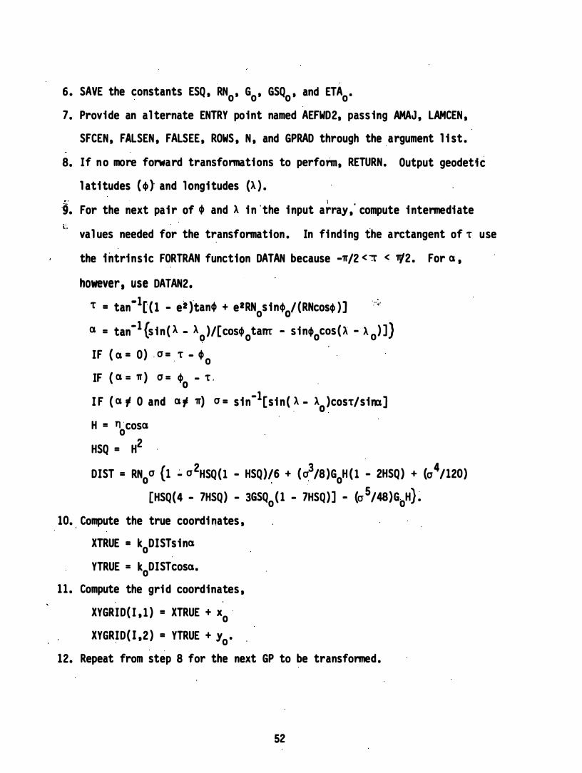
6 . SAVE the constants ESQ , RNo ' Go ' GSQo ' and ETAo.

7. Provide an al ternate ENTRY point named AEFWD2, pass ing AMAJ , LAMCEN ,

SFCEN , FALSEN , FALSEE , ROWS , N , and GPRAD through the .argument l i st .

8. If no more forward transformations to perform, RETURN. Output geodetic

l atitudes (�l and l ongitudes (A ) .

·9. For the next pai r of , and A i n ' the i nput a�ray ,' compute i ntermediate

t. val ues needed for the transfonnation . In finding the arctangent of t use

the hltr1ns1c FORTRAN funct10n DATAN because -Tf/2 < "l' < Tr/2. For a ,

however, use DATAN2.

t = tan-1[U - et han' + e2RNos in'0/ (RNcos, )] .:'.'

a = tan-1 {s i n ( A - Ao )/[cos'otam - s in,ocos ( x - A O) ]) IF ( a = O) . o = . t - ,o IF ( a = Tf ) o = 'o - t .

I F ( a rI 0 and a rl '11') 0 = s 1n-1[si n ( A - A )cost/sirn] . 0 H = n · cosa o HSQ = H2 .

DIST = RNoo {I � 02HSQ(1 - HSQ)!6 + ( �3/8)GoH ( 1 - 2HSQ) + (04/120)

[HSQ(4 - 7HSQ) - 3GSQo( 1 - 7HSQ)] - (0 5/48)GoH) �

10. Compute the true coordi nates ,

XTRUE = koDISTsina

YTRUE = koDISTcosa.

1 1 . Compute the grid coordinates ,

XYGRID( I , l ) = XTRUE + xo .

XYGRID( I ,2 ) = YTRUE + Yo .

12. Repeat from step 8 for the next GP to be transformed.

52

Reference :

Snyder, 1983 , pp . 188-189.

Azimuthal Equidi stant Inverse Transformation (AEINV )

Input :

AMAJ

FINV

LAMCEN

PHICEN

SFCEN

FALSEN

FALSEE

ROWS

Semimajor axi s of el l ipsoid ( a ) .

Reci procal of fl atteni ng ( l/f) .

Central meridian ( AO ) . Geodeti c l ati tude of the center point (�o ) .

Scal e factor at the center poi nt (for the case at hand , a

cartographic scale factor) ( ko ) .

Fal se northi ng (Yo ) .

Fal s� easting (xo) .

Number of rows declared for the arrays GPRAD and XYGRID i n the

cal l i ng program.

N Number of positions to . be transformed.

XYGRID( I , l ) · x coordinate , relative to the grid origi n , of the ith posi tion

to be transformed .

XYGRID( I ,2) y coordinate relati ve . to the grid origin.

Output :

GPRAD( I , l )

GPRAD( I ,2 )

Geodeti c l atitude , in radians , of the transformed ith posi tion (� ).

Longi tude of the posi tion (A ) .

53

Other meaningful · variables:

FLAT

ESQ

E·2SQ

El l ipsoidal flattening (f) . Fi rst eccentrici ty of el l ipsoid , squared (el ) .

Second eccentricity squared (e ' l ) .

. . E TASQ

:RN

·RNCEN -

DIS T

All

Geodetic variable (Il l ) representing the quantity e ' lcosl� •

Rad'us of curviture in the prime vertical .

RN at the center point (RNo) .

Geodetic distance between center point and point i n question.

Geodetic azimuth , measured clockwise from north , of the normal

section from the central point to the point in question (B ) • •

TAU Isometric l atitude (T ) .

JTRUE x coordinate rel ative to the true origin of the projection .

Y TRUE y coordinate relative to the true origin.

Algorithm:

·.1 . Input el l i psoid parameters AMAJ and FINV.

2 . Input projection parameters LAMCEN , PH ICEN ,·SFCEN, FALSEN , and

FALSEE.

3. Input ROWS , N , .and array XYGRID.

4. Compute el l i psoidal constants ,

f • 1/(1/f)

el • f(2 - f)

e ' l - el/(1 - el ) .

5 . CoInpute co.nstants needed for the transfonnation ,

RN • 1/(1 - elsinl «k )1 o . 0 ·flo I · e I ICOSI�O.

54

6. SAVE the· constants ESQ , E2SQ , RNo and ETASQo . 7 . Provide an al ternate ENTRY poi nt named AEINV2 , passing AMAJ , LAMCEN ,

SFCEN , FALSEN , FALSEE, ROWS , N , and XYGRID through the argument l i st. 8. If no more i nverse transfonnati ons .to perform, RETURN . Output geodetic

lati tudes ( �) and l ongi tudes (A ) .

9 . For the next pa; r of gr;d coord; nates ;n the ;nput array . compute intermediate val ues needed for . the transformation . In finding the arctangent of a , use the " i ntrinsi c FORTRAN functi on DATAN2 . For 4> use DATAN because - '0/2 , 4> 'n/2.

XTRUE = x - xo YTRUE = y - Yo DIST = (XTRUE2 + YTRUE2 )i/ko a = tan-1 ( XTRUE/YTRUE) A = "110 2cos2 a 8 = 3e · 2( 1 + A)sin4>oco�ocosa D = DIST/RNo E = D + A( l - A)D3/6 - 8( 1 - 3A)D4/24

F = 1 + A(E2/2 ) - 8( E3/6 ) L = s in-1 ( s i n4>oCOSE + cos4>osinE coSa ) .

10. Compute the geodeti c l ati tude (4) ) and longi tude (A ) ,

� = tan-1[ (tanL - e2FSin�0/cosL )/ ( 1 - e2 ) ] A = A o "+ s in-� (S inasinE/cosr ) IF (). . � -'It) GPRAD( I ,2) = ). + 21T I F (A > � GPRAD( I ,2 ) = ). - 2'If .

1 1 . Repeat from step 8 for the next pai r · of xy coordinates to be transformed.

55

Reference :

S�der, 1983 , pp . 19l-192.

Datum Transfonnation

Geodetic Datums

�A cl assical horizontal geodeti c datum i s simpl e i n concept . It i s a mathematical surface , an el l i psoid , oriented by defi nition to the topographi c sUrface of the Earth . On an ideal planet . survey observations could be entered di rectly i nto an el l i psoidal model of the Earth , and accurate posi tions would be obtained .

In real i ty , survey observations are affected by the distribution of mass wi thin the Earth . . Instruments used in classical geodeti � surveyi ng are oriented to the Earth by -gravity ,· ;which i s i rregular dlle�tto uneven di'stribution of mass . Observations are therefore "ti l ted" at varyi ng degrees

. wl:th respect to the el l i psoid . The ti l t i s gi ven i n geodeti c tenns as " deflection of the verti cal " . Additional ly , position computations must account for the i rregular topography over which the observations were obta; ned.. Thus . the mathemat; ca 1 surface upon whi ch position computations are made i s ·'only a good approximation of the physi cal Earth . .

.:·A mi nimum of five parameters are needed to defi ne · a geodeti c datum. Two ·of the parameters define the s ize and shape of the el l i psoid . Length of the semimajor axi s and el l i psoidal fl attening are commonly used . The other three p�rameters are l atitude and l ongi tude of a ,survey monument used as a starti ng poi nt (or geodeti c origi n ) , and azimuth from the ori gi n to another nearby monument. The l atter three parameters coul d · be ass.i gned arbitrari ly·, but i n practi ce they are usual ly detenni ned by astronomic observations . Si nce they are detennined by ·; observation . they are i nfl uenced by gravi ty and topography by �n amount that can be detenni ned only wi th further observations .

If the. ori gin happened to be l ocated where el evation was known and where the gravity field behaved favorably� the datum woul d be a fai rly good one . Defl ection of the vertical at other survey poi nts throughout the region i n whi ch the datum was employed woul d tend to average out. More typical ly , gravity anomol ies exist i n the vicinity of the origin . Wi th the resul ts of a prel iminary survey , a deflection of the vertical can be assi gned to the ori gin , whi ch wi l l _minimize deflection of the vertical averaged for survey poi nts throughout the region .

Deflection of the vertical i s quantified in two ways , each requi ri ng two parameters . Either a total deflection and an azimuth i n the d irection of maximum defl ection , or components of the deflection i n a north-south ( prime meridian ) and east-west (prime verti cal )" di rection can be used . : The parameters defin ing the defl ection of'··the verti'·ca·l at the ·orig in , al ong with the other five parameters di scussed earl ier , amount to seven parameters . c lassical ly used to define a geodeti c datum.

56

Defi nition of a geodeti c datum can be seen as an iterative procedure. The seven defini ng parameters provide the basi s for computation of al l other positions i n the network . As geodeti c and astronomic pos itions of more and more survey poi nts a� determined , they can be used to redefine the deflection of the vertical at the orig in , thereby making the datum more closely fi t the p�sical Earth . A geodetic datum. therefore , might be defined as the l ocus of al l monumented points in the geodetic network rather than a l i st of seven p�rameters .

Three concl usions drawn from thi s di scussion wi l l hel p i n the understandi ng of datum transformations :

1 . · Class i cal geodeti c datums are desi gned to fit a particu lar region . A datum that i s suitable for one region might not be sui table el sewhere.

2 . A geodetic datum i s not necessari ly geocentri c , but in a wel l ­designed datum the equatorial pl ane of the el l i psoid i s nearly coi ncident wi th the equatorial pl �ne of the Earth , and the mi nor axi s of the el l ipsoi d i s nearly paral lel wi th the average spin axi s of the Earth . Thi s i s because astronomic observations interspersed throughout the network hel p define the orientation of the reference el l i psoid .

3. Because the geodeti c datum can be thought of as the l ocus of al l monumented poi nts i n the regional network , each subset of poi nts . i .e . , an area wi thin the region , can be thought of as defi ning a sl i ghtly different datum.

Space Coordinates

A space coordinate system i s simply a three-dimensional system of Cartes ian coordinates . When used for satel l ite surveying , the ori gin of the XVZ space coordinate system i s l ocated at the Earth ' s center of mass , providing truly . geocentric coordinates . For our purposes the origin of the XVZ coordi nate system i s l ocated at the center of the reference el l i psoi d upon which a geodetic datum i s based . It may or may not be truly Earth-centered. The XV plane of the system i s coi ncident wi th the equatorial pl ane of the el l i psoid , the I axi s i s coi ncident with the minor axi s of the el l i psoid , and the Xl plane contains · the meridian of zero l ongi tude . .

Transformation Overview

There are many approaches to performing datum transformations . The fol l owing scheme i s used here : .

1 . Geodetic coordinates i n the "old" datum are converted to o l d XYI coordi nates .

2 . The old XVI coordinates are transformed to "new" XYI coordi nates . The XYI coordinate transformation invol ves a transl ation of the orig in . rotation of the axes . and a scale change.

3. The new XVI coordinates are converted to geodetic coordi nates i n the new datum.

The conversion ·of geodeti c coordinates to XVI coordinates i n step 1 requi res knowl edge of the hei ght of the poi nt in question above the el l ipsoid . Height

57

above the el l ipsoid i s the sum of orthometric height (el evation above spa l evel ) and geoidal separation . For cartographic appl ications , geoidal hei ght , if unknown , can be assumed to be O.

The transformation of original XYI coordinates to new XYI coordinates is the crux of the ,prOblem. There are a number of ways to accompl i sh thi s . The method di scussed here i s the Bursa-Wol f model .

where

x

Y

I new

('� , Il Y , Ill ) 0

00, £ , and IP

Ilk

= 1 00 -lP

Il Y + -00 1 £

Il I 0 IP - £ 1

x

Y

I ol d

( 1 + Il k )

a re the components of transl ation of the ori gi n (new minus old) are rotations about the I , X and Y axes , respectively i s the change i n scal� .

rhe rotation matrix i n the Bursa-Wol f model i s an approximation , making use of ' the fact that 00 , £ , and IP are smal l ; therefore th� si nes of these angl es are approximately equa l to the angl es themsel ves , the product of the s ines approximately equal 0, and the cosi nes approximately equal 1 . Carrying out the mul ti pl ication and rearrangi ng , the fol l OWi ng equations are obtained :

Xn = , � + (Xo + 00 Yo - lPlo ) ( l + Il k ) Yn = IlY + (Yo - WXo + £lo ) ( 1 + Il k ) In =, III + (lo + IPXo - £Yo ) ( l + Il k )

where subscr1'pts n and 0 denote new and old .

IlX , Il Y , Il l , w , £ , IP , and Ilk are seven transfonnation parameters needed to compute new X ' s , Y " s , and l ' s . Thei r val ues are detenni ned by a l east squares method in which the model i s suppl ied with known coordinates in the o ld and new coordinate systems . In practi ce i t i s di fficul t to detenmine the correct combination of trans lation , rotation , ' and scale change . If the geodeti c datum was devel oped wi th care , w , and especial ly £ and IP are i ndeed very smal l , i ndicating the reference el l i psoid i s properly oriented to the physi cal Earth. Smal l rotation angles compl i cated by di stortions i n the geodeti C network make i t practical to consider datum shifts i n subregions of a geodetic network to be caused enti rely by transl ation of XYI origins . Thi s argument i s supported by conclusion 3 , above.

Estimated val ues of IlX , Il Y , and III to prel iminary NAD 83 have been computed by the National Geodetic Survey for stations i n the Uni ted States . Mean shifts ca l culated from these val ues a're li sted i n appendix, C . Mean shifts rel ating other l ocal datums to the World Geodetic System of 1972 (WGS 72) have been tabul ated by , the Defense Mappi ng Agency Hydrographic/Topographic Center,

58

Geodesy and Surveys Department (DMATC) (AYres 1983 ) . To transl ate coordi nates from these l ocal datums to NAD 83 . add A X = O. I:J. Y = O . and I:J. Z = 4 . 5 meters to the DMATC parameters used to obtain WGS 72 coordi nates . Shifts of hydrographic posi tions at sea are assumed to be t�e same as the shifts along the coast where the shore control was l ocated .

Note wel l that the datum transformation thus obtained i s general ly not suitabl e. for preci se positioning , but can be safely used i n cartographic appl ications . If w • t ' lP • and I:J.k are suppl ied , and i f the elevation and geoidal separation are known . the transfonmation can be used for geodetic appl ications .

Input :

AMAJ

FINV

DELTAX

DELTAY

DELTAZ

OMEGA

Semimajor axis of el l i psoid (a ) .

Reci procal of fl atteni ng ( l/f) .

Transl ation i n the X di rection i n the sense new mi nus ol d (A X ) .

Transl ation i n the Y di rection . i n the sense new minus ol d (I:J. Y ) .

Translation i n the Z di rection i n the sense new minus ol d (I:J. Z ) .

Angle of rotation of the in itial XYZ system about the Z axis ,

positive i n the counter-clockwi se di rection as preceived from

positive Z toward the origin (w) .

EPSIL Angl e of rotation in same sense as w , about the X axi s after w

has been appl ied (£ ) • .

PSI Angl e of. rotatfon . i n same sense as w. about the Y axi s after w

and £. have been appl ied (1P ) . DELTAK

ROWS

N

Change i n scale factor i n the sense new minus ol d (l:J.k ) .

Number of ro�s decla.red .for the arrays GPORAD and GPNRAD in the

cal l ing program.

Number of positions to be transformed .

GPORAD ( t. l ) Old geodetic l atitude . i n radians , of the ith position to be

transfonmed (410 ) . GPORAD( I .2) O l d longitude of the posi tion (Ao) .

59

" ELEV ( I ) " . Elevation (orthometri c hei ght) of the i th p�si tion (H) . NSEPO( I ) Geoidal separation of the ol d datum at the i th pos i ti on (NSEPo ) .

Output : "

tPNRAD( I , l ) New geodeti c l ati tude , i n radians , of the transformed i th

posi ti on ( 4)n ) . 'GPNRAD( 1 ,2 ) HTO( I ) HTN( I ) NSEPN( I )

' New l ongi tude of posi tion (An ) . Height of the i th posi tion above the o ld el l i psoid ( ho ) . Height of the i th posi tion above the new el l i psoi d ( hn ) . Geoidal separation of the old datum at th� ith posi tion (NSEPn ) .

Other Meani ngful Variables : , "

FLAT El l i psoidal fl atteni ng (f) . BMIN Semimi nor axi s of el l i psoi d (b ) . ESQ Fi rst eccentri c ity of el l i psoid , squared (e2 ) . �E2SQ Second eccentric ity squared (e I 2 ) . RN Radi us of curvature i n prime verti cal . Suffixes 0 and N denote "ol d" and "new" .

Al gori thm: 1 . Input el l i psoid " parameters AMAJO . FINVO . AMAJN , and " FINVN. 2 . Input transformation parameters DELTAX , DELTAY , DELTAZ , OMEGA . EPS IL ,

PS I . and DELTAK. 3. Input ROWS , N . and arrays GPORAD ELEV . and NSEPO.

60

4. Compute el l i psoidal constants ,

fo = l/ ( 1/fo )

f n' = 1/ ( 1/fn )

bn = an ( 1 - fn)

e 2 = 2f - f 2 0 0 0

e 2 = 2f - f 2 n n n

en " = en'/( l - en' ) ·

5. SAVE the constants FLATO. FLATN . BMINN . ESQO , ESQN an� E2SQN.

6. Provide an al ternate EN�RY point named DATUM2 , passing AMAJO. AMAJN .

DELTAX . DELTAY . DELTAZ . OMEGA, EPSIL. PSI . DELTAK, ROWS , N , GPORAD , ELEV ,

and NSEPO through the argument l i st .

7 . If no more transformations to perform. RETURN . Output new geodetic

latitudes (�n ) ' l ongi tudes (� ) . el l ipsoidal heights (ho and hn ) , and

geoidal separations (NSEPn ) .

8. For the next set of cjlo ' >. 0 ' and ho in the input arrays , compute the

radi us of curvature and height above el l i psoid in the ol d system,

RN = a/ ( l - e2sin2cj1 ) 1 o 0 ho � H + " NSEPo•

9 . Compute Cartesian coordi nates in the ol d system,

Xo = (RNo + ho ) coscjlo cosAo Yo = (RNo + ho ) cOScjlo sin>.o Zo = [RNo ( l - e02 ) + hol sin cjlo ·

10. Transform the Cartesian coordi nates from the ol d to the new · system,

Xn = �X + (Xo + w Yo - w Zo ) ( 1 + �k) Y n = 6 Y + (Yo

- w Xo + e20) ( 1 + 6 k)

Zn =. 6Z + ( Zo + wXo - eVo ) (1 + � k ) .

61

1 1 . Compute geodeti c coordi nates in the" ,new datum, us�ng the DATAN2 function

for cal culati ng A ,

P = (X 2 + Y 2)i n n

e = tan -l[anzn/ (bnP ) ]

� = tan-1[ ( Z + e . 2b s in3e )i (p - e 2a cos3e ) ] �n ' n n n n n A n EI tan-1 (yn/xn)

I F (An <. -1T) " GPNRAD( I ,Z) = An + Z1T I� (Xn > on: ) GPNRAD( I ,2) = A n - 21T

RN = a / ( 1 - e 2sin2cp )i n n n n

hn • p/cOS4>n - RNn NSEPn = hn - H.

lZ. Repeat from step 7 for the �ext GP to be transformed.

Reference's :

1 . Rapp . 1981 . pp. 53-57 . 66.

2. Bowring , 1976, p�. 323-327.

62

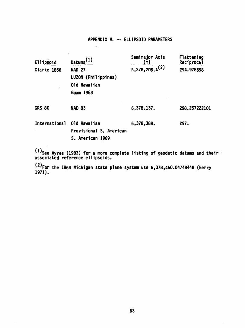
APPENDIX A. -- ELL IPSOID PARAMETERS

El l i2S0id Datums ( l ) Semimajor Axis Fl atteni ng {ml Rec12rocal

Clarke 1866 NAD 27 6 ,378 ,206 . 4(2) 294. 978698 LUZON ( Phi l i ppi nes ) Ol d Hawai i an Guam 1963

GRS 80 NAD 83 6 ,378 , 137 . 298. 257222101

International Old Hawai ian 6 ,378 ,388. 297 . Provi sional S. American. S . American 1969

( 1 )See AYres ( 1983 ) for a more compl ete l i sti ng of geodeti c datums and thei r · associated reference el l i psoids . ( 2 )For the 1964 Michi gan state pl ane system use 6 ,378 ,450 .04748448 (Berry 1971 ) .

63

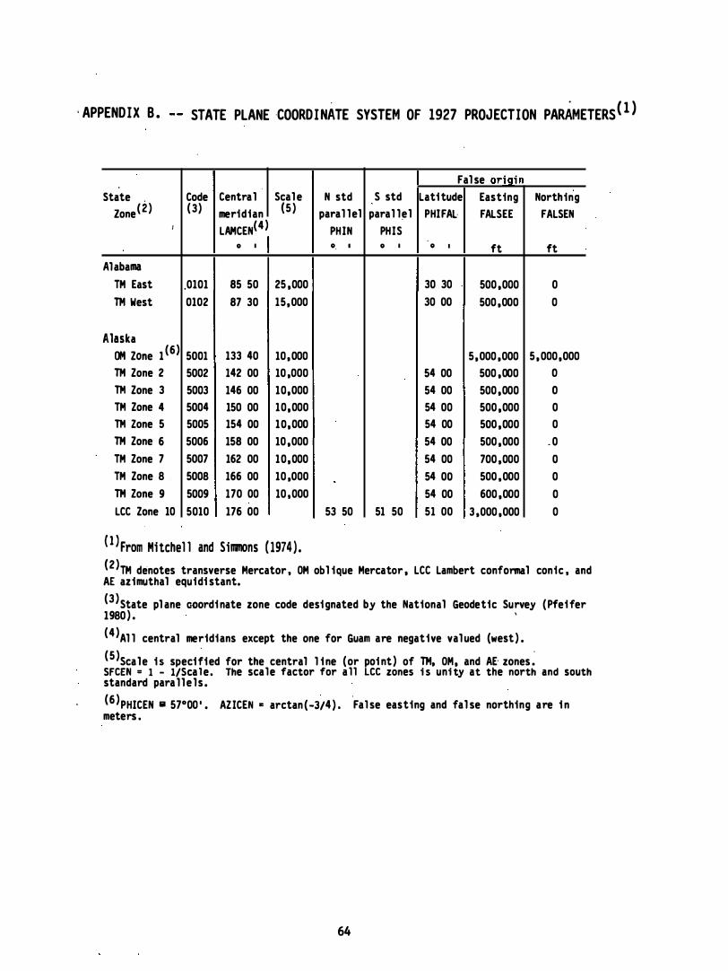
' APPENDIX B . STATE PLANE ·COORDINATE SYSTEM OF 1927 PROJECTION PARAMETERS( l )

Fal se oriJlin State Code Central Scal e N std S std Lati tude Easting Northing

zone( 2 ) ( 3) meridian (5 ) paral lel paral lel PHIFAL FALSEE FALSEN I LAMCEN(4 ) PHIN PHIS

° , ° , ° , ° , ft ft Alabama

TM East .0101 85 50 25 .000 30 30 500 .000 0 TM West 0102 87 30 15.000 30 00 500 .000 0

Alaska OM Zone 1 (6) 5001 133 40 10.000 5.000 .000 5 .000.000 TM Zone 2 5002 142 00 10 .000 54 00 500 .000 a TM Zone 3 5003 146 00 10.000 54 00 500 .000 a TM Zone 4 5004 150 00 10.000 54 00 500 .000 0 TM Zone 5 5005 154 00 10.000 54 00 500 .000 0 TM Zone 6 5006 158 00 10 .000 54 00 500 .000 . 0 TM Zone 7 5007 162 00 10.000 54 00 700 ,000 0 TM Zone 8 5008 166 00 10 ,000 54 00 500 ,000 0 TM Zone 9 5009 170 00 10 ,000 54 00 600 .000 0 LCC Zone 10 5010 176 00 53 50 51 50 51 00 3 .000 .000 0

( l ) From Mi tchel l and Simmons ( 1974 ) . (2 )TM denotes transverse Mercator , OM obl ique Mercator . LCC Lambert conformal conic , and AE azimuthal equidi stant.

(3 )State pl ane GOordi nate zone code desi gnated by the National Geodetic Survey ( Pfei fer 1980 ) . '

(4 )Al l central meridians except the one for Guam are negative val ued (west ) .

( 5 )Scale i s speci�ied for the central l i ne (or poi nt ) of TM. OM. and AE· zones � SFCEN = 1 - l/Scale . The scale factor for al l LCC zones i s uni ty at the north and south standard para l l e l s .

(6 )PHICEN a 57°00 ' . AZICEN E arctan ( -3/4 ) . Fal se easting and fal se northing are i n meters .

64

State Code Central Scal e N std S std Zone (2 ) ( 3 ) meridian ( 5) paral lel paral lel

LAMCEN(4) PHIN PHIS 0 I 0 I 0 I

Ameri can Samoa LCC 170 00 -14 16 -14 16

Ari zona TM East 0201 1 10 10 10,000 TM ,Central 0202 1 1 1 55 10 ,000 TM West " 0203 113 45 ' 15 ,000

Arkansas LCC North . 0301 92 00 36 14 34 56 LCC South ' 0302 92 00 34 46 33 18 I

Cal i fornia LC� Zone 1 0401 122 00 41 40 40 00 LCC Zone 2 0402 122 00 39 50 38 20 LCC Zone 3 0403 120 30 38 26 37 30 LCe Zone 4 0404 119 00 37 15 36 00 LCC Zone 5 0405 ' 118 00 35 28 34 02 LCC Zone 6 0406 116 15 33 53 32 47 LeC Zone 7 0407 118 20 34 25 33 52

Col orado LCC North 0501 105 30 40 47 39 43 Lee Central 0502 105 30 39 45 38 27 LCC South 0503 105 30 38 26 37 14

Connecticut LCC 0600 72 45 41 52 41 12

Del aware TM 0700 75 25 200 ,000

(7 ) FALSEE • 4 , 186 ,692 . 58. FALSEN · 4 , 160 ,926 . 74.

65

Fal se origin LatHude Easting North i ng

PHI FAL FALSEE FALSEN

0 I ft ft --- 14 16 . 500 ,000 312 ,234.65

31 00 500 ,000 0 31 00 500 ,000 0 31 00 500 ,000 0

34 20 2 ,000 ,000 0 32 40 2 ,000,000 0

39 20 2 ,000 ,000 0 37 40 2 ,000 ,000 0 36 04 2 ,000 ,000 0 35 20 2 ,000 ,000 0 33 30 2 ,000,000 0 32 10 2 ,000 ,000 0 34 08 ( 7 ) ( 7 )

39 20 2 ,000 ,000 0 37 50 2 , 000 ,000 0 36 40 2 ,OCO ,OOO 0

40 50 600 ,000 0

38 00 500 ,OCO 0

Fal se origin State Code Central Scale N std S std Latitude Easting Northi ng

Zone( 2 ) (3 ) meridian (5 ) paral lel paral lel PHIFAL FAlSEE FALSEN LAMCEN(4) I PHIN PHIS

0 1 0 1 0 1 0 1 ft ft Fl orida

1M East 0901 81 00 17 ,000 24 20 500 ,000 0 1M West 0902 82 00 17 ,000 . 24 20 500 ,000 0 LCC North 0903 84 30 30 45 29 35 29 00 2 ,000 ,000 0

Georg;a 1M East 1001 82 10 10,000 30 00 500 ,000 0 1M West 1002 84 10 10 ,000 30 00 500,000 0

Guam(8) AE Exact . . 50 ,000 50 ,000

HawaH 1M Zone 1 5101 155 30 30,000 18 50 500 ,000 0 1M Zone 2 · 5102 156 40 30,000 20 20 500 ,000 0 1M Zone 3 5103 158 00 100 ,000 21 10 500 ,000 0 1M Zone 4 5104 159 30 100 ,000 21 50 500 ,000 0 1M Zone 5 5105 160 10 Exact 21 40 500 ,000 0

Idaho 1M East 1 101 ' 112 10 19,000 , 41 40 500 ,000 a 1M Central 1102 114 00 19 ,000 41 40 500,000 0 1M West 1 103 115 45 15 ,000 41 40 500 ,000 0

I 1 H nois 1M East 1201 88 20 40,000 36 40 500 .000 0 1M West 1202 90 10 17 ,000 36 40 500 .000 0

Indiana 1M East 1301 85 40 30 ,000 37 30 500 ,000 0 1M West 1 302 87 05 30 .000 37 30 500,000 0

(8)Fal se easti ng and fal se northing are i n meters . LAMCEN . east (+ ) 144044 1 55. 50254" . PHICEN • north 13D28 1 20.87887" •

66

Fal se ori!lin State Code Central Scale N std S std Lati tude Easting North i ng

Zone ( 2) (3) meridian (5 ) paral l el paral lel PHIFAl FALSEE FAlSEN LAMCEN(4) PHIN PHIS

0 I 0 I 0 I 0 I ft ft Iowa

LCC North 1401 93 30 43 16 42 04 41 30 2. 000.000 0 LCC South 1402 93 30 41 47 40 37 40 00 2 .000 .000 0

Kansas LCC North 1501 98 00 39 47 38 43 38 20 2 ,000 .000 0 LCC South 1502 98 30 38 34 37 16 36 40 2 .000 ,000 0

Kentucky LCC North 1601 84 15 38 58 37 58 37 30 2 .000 .000 0 LCe South 1602 85 45 37 56 36 44 36 20 2 . 000 .000 0

Loui s,tana Lee North 1701 92 30 32 40 31 10 30 40 2 .000 ,000 0 Lee South 1702 91 20 30 42 29 18 28 40 2,000 ,000 0 lCe Offshore 1703 91 20 27 50 26 10 25 40 2 .000 ,000 0

\

Maine TM East 1801 68 30 10 .000 43 50 500 .000 0 TM West 1802 70 10 30 ,000 42 50 500 .000 0

Maryland Lee 1900 77 00 39 27 38 18 ' 37 50 80C.000 0

Massachusetts lec, Mainland 2001 71 30 42 41 41 43 41 JO 600 .000 0 leC Island 2002 70 30 41 29 41 17 41 00 200.000 0

Mi,chtgan ( 1934 ) TM East 21(il 83 40 17 .500 41 30 500 .000 a TM Central 2102 85 '45 11 ,000 41 30 500 .000 0 TM West 2103 88 45 11 .000 41 30 500 .000 0

67

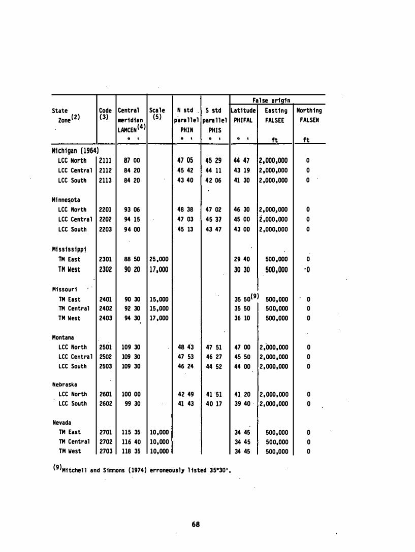
State Code Zone(2) (3)

Mi chi gan ( 1964)

LCC North 2111

LCC Central 2112 Lee South 2113

Mi nne�ota Lee North 2201 Lee Central 2202 LeC South 2203

Mi ssissipp1

TM East 2301 TM West 2302

Mi ssouri .

TM East 2401 1M Central 2402 1M West 2403

Montana LCe North 2501-LCC Central 2502 LCC South 2503

Nebrask.a LCC North 2601 LCC South 2602

Nevada 1M East 2701 1M Central 2702 1M West 2703

Central Scale

meridian (5 ) LAMCEN (4 )

0 ,

87 00 84 20 84 20

93 06 94 15 94 00

88 50 25 .000 90 20 17.000

90 30 15.000 92 30 15 .000 94 30 17 .000

109 30 109 30 109 30

100 00 99 30

115 35 10 .000 116 40 10.000 118 35 10.000

N std .

paral lel

PHIN 0 ,

47 05

45 42 43 40

48 38 47 03 45 13

48 4·3 47 53 46 24

42 49 41 43

S std

paral lel

PHIS 0 ,

45 29

44 11 42 06

47 02 45 37 43 47

47 51 46 27 44 52

41 '51 40 17

(9)Mi tchel l and Simons ( 1974) erroneously l isted 35°30 ' .

68

Fal se origin

latitude Easting Northing

PHIFAL FALSEE FALSEN

0 , ft ft

44 47 ?,OOO,OOO ·0 43 19 2 ,000,000 0 41 30 2 .000 .000 0

46 30 2 .000 .• 000 0 45 00 2 .000 .000 0 43 00 2 .000.000 0

29 40 500 .000 0 30 30 500 .000 ·'0

35 50(9) 500.000 0 35 50 500.000 0 36 10 500 .000 0

47 00 2 .000.000 0 45 50 2 .000 .000 0 44 00 2 .000.000 0

41 20 2 .000.000 0 39 40 . 2 .000 .000 0

34 45 500.000 0 34 45 500.000 0 34 45 500 .000 0

Fal se origfn State Code Central Scale N std S std Lati tude East ing Northins;

Zone( 2) ( 3 ) meridian ( 5 ) para l l el paral lel PHI FAL FALSEE FALSEN lAMCEN(4) PHI N PHIS

0 I 0 I 0 I 0 I ft ft New Hampshire

TM 2800 71 40 30 ,000 42 30 500.000 0

New Jersey TM 2900 74 40 40 ,000 38 50 2 ,000 .000 0

New Mexi co TM East 3001 104 20 11 ,000 31 00 500 ,000 0 TM Central 3002 106 15 10,000 31 00 500 ,000 0 1M West 3003 107 50 12,000 31 00 500 .000 0

New York LCC Long I s . 3104 74 00 41 02 40 40 40 30 2 ,000 ,000 100 , 000 TM East 3101 74 20 30 ,000 40 00 500,000 0 1M Central 3102 76 35 16 .000 40 00 500 ,000 0 TM West 3103 78 35 16,000 40 00 500 .000 0

North Ca ro 1 ina LCC 3200 79 00 36 10 34 20 33 45 2 .000 ,000 0

North Dakota LCC North 3301 100 30 48 44 47 26 47 00 2 , 000 ,000 0 LCC South 3302 100 30 47 29 46 1 1 4 5 40 2,000 ,000 0

Ohio LCC North 3401 82 30 41 42 40 26 39 40 2,000 .000 0 LCC South 3402 82 30 40 02 38 44 38 00 2 ,000 .000 0

Oklahoma LCC North 3501 98 00 36 46 35 34 35 00 2 .000 ,OOC 0 LCC South 3502 98 00 35 14 33 56 33 20 2,OOO ,OOC 0

69

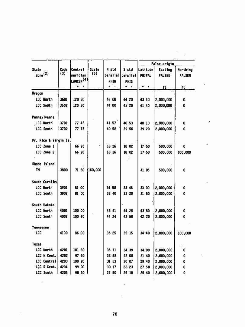
Fal se origin State Code Central Scale N std S std Latitude Easting Northing

Zone(2) (3) meridian (5) paral lel para l l el PHIFAL FALSEE FALSEN LAMCEN (4 PHIN PHIS

0 I 0 I 0 I 0 I ft ft Oregon

LCC North 3601 120 30 46 00 44 20 43 40 2,000,000 O. LCC South 3602 120 30 44 00 42' 20 41 40 2,000,000 0

Pennsylvania LCC Nortti 3701 77 45 41 57 40 53 40 10 2,000 ,000 0 LCC South 3702 77 45 40 58 ' 39 56 39 20 2 ,000,000 0

Pro Rico & V;rgin Is . LCC Zone 1 66 26 18 26 18 02 17 50 500,000 0 LCC Zone 2 66 26 18 26 18 02 17 50 500 ,000 100 ,000

Rhode Isl and TM 3800 71 30 160,000 41 05 500 ,000 0

South Carol im LCC North 3901 81 00 34 58 33 46 33 00 2,000,000 0 LCC South 3902 81 00 33 40 32 20 31 50 2,000,000 0

' South Dakota LCC North 4001 100 00 45 41 44 25 43 50 2 ,000,000 0 LCC South 4002 1QO 20 44 24 42 50 42 20 2,000,000 0

Tennessee LCC 4100 86 00 36 25 35 15 34 40 2,000 ,000 100 ,000

Texas LCC North 4201 101 30 36 11 34 39 34 00 2,000,000 0 LCC N Cent. 4202 97 30 33 58 32 08 31 40 2,000 ,000 0 LCC Central 4203 100 20 31 53 30 07 29 40 2 ,000,000 0 LeC S Cent. 4204 99 00 30 17 28 23 27 50 2 ,000 ,000 0 LCC South 4205 98 30 27 50 26 10 25 40 2,000,000 0

70

State Code Central Scale N std

Zone(2) (3) meridian (5 ) paral lel

lAMCEN (4) PHIN 0 , 0 I

Utah LCC North 4301 111 30 41 47 LCC Central 4302 111 30 40 39 LCC South 4303 III 30 38 21

Vennont TM 4400 72 30 28 .000

Vi rginia Lee North 4501 78 30 39 12 · LCe South 4502 78 30 37 58

Washi ngton Lee North 4601 120 50 48 44 LCC South 4602 120 30 47 20

West V irginia Lee North 4701 79 30 40 15 Lee South 4702 81 00 38 53

Wi sconsi n Lee North 4801 90 00 46 46 LCC Central 4802 90 00 45 30 leC South 4803 90 00 44 04

Wyoming TM Zone I 4901 105 10 17 ,000 TM Zone I I 4902 107 20 17.000 TM Zone I I I 4903 108 45 17.000 TM Zone IV 4904 110 05 17 ,000

7 1

S std

paral lel

PHIS 0 I

. 40 43 39 01 37 13

38 02 36 46

47 30 4S 50

39 00 37 29

45 34 44 15 42 44

Fa he orilli n

Lati tude Easting Northing PHI FAL FALSEE FALSEN

D I ft ft

40 20 2 .000 .000 0 38 20 2 .000 .000 0 36 40 2 .000 .000 0

42 30 500 .000 0

37 40 1 2 .JOO ,OOO . 0 36 20 2 . 000,000 0

!

47 00 2 .000.JOO 0 45 20 2 .000 .300 0

38 30 2 .000 .000 0 37 00 2 .000,000 0

45 10 2 ,000 .000 0 43 50 2 .000 , 000 0 42 00 2 .000,000 0

40 40 500 .000 0 40 40 500 .000 0 40 40 500.000 J 40 40 500.000 0

APPENDIX C . -- XYZ COORDINATE TRANSLATION PARAMETERS( I )

NAD 27 TO PRELIMINARY NAD 83

Del ta X Del ta Y Del ta Z Area 'ml 'ml 'ml

Conti guous Uni ted States Mai ne 23. 1 - 16 1 . 0 " -187 . 5 Massachusetts 19. 1 - 161 . 5 -189.2 Gape May 17. 5 -16 1 . 4 -186.8

Vi rginia 15. 5 -158. 4 -186. 1

Paml ico Sound 12. 8 -161 . 5 - 187 . 2

Cape Fear 15. 0 -157 . 2 -182 . 3

South Carol ina 17 . 0 -154. 0 - 180 . 3

Georgia 1 1 . 8 -152 . 4 -181 . 9

F.� ori da (peninsula ) 1 1 . 6 -153 . 6 -178 . 5

Fl ori da ( panhandl e) 12.2 -150. 6 -175 . 7 Mi ss 1ss 1pp1 Del ta 15. 5 -150.8 -176. 0 Texas 15 . 6 -150. 8 -178 . 3

Cal i fornia San Diego area 2 1 . 4 - 153.8 -180. 9 Los Angeles area 22. 5 - 154. 2 -182 . 3

Santa Maria 25. 4 -155. 6 -ld2 . 2

Monterey a rea 24. 1 - 158. 5 -186 . 7 San Francisco area 22. 8 -158. 3 -187 . 3

" Ukiah to Eureka 22 . 7 - 156.8 -188.4

Klamath 19. 3 - 161. 4 -182.9 Washi ngton 18. 7 -157 . 1 -187 . 4

Alaska Southeast Al aska

Shoal Cove 17 . 6 -154 . 6 -182 . 9

Craig 13.4 -151 . 0 -182 . 6

Wrangel l to Biorka Isl and "13. 9 �146 . 4 -180. 2

Juneau 10. 3 -145 . 1 -181 . 3

( I ) For coa�tal areas . Ori ginal data furni shed by Astrono� and Space Geodesy Section , National Geodetic Survey, NOAA. Some val ues represent averages for the area; othe"rs a'1! : for s ingl e stations i n the area .

72

Del ta X Delta Y Del ta Z Area (m) . (m) (m) -

Southeast Alaska (conti nued) Hai nes 9 . 9 -143 . 6 -180. 9

Yakutat Irregular Southern Al aska

Cape Yakataga -0. 8 -134. 1 -184 . 7

Prince· Wi l l iam Sound 11 . 7 -130 . 3 -177 . 3

Anchorage and Kenia Peninsula (exe. Nuka Island) . 10.8 -136 . 9 - lS0. 7

Nuka Island 17. 4 -131 . 9 -176 . 1

kamishak Bay 1 1 . 5 -137 . 0 -181 . 1

Kodiak Isl and Irregular Alaska Peninsula

king Salmon Irregular Port Heiden 2 1 . 6 - 149. 6 -179 . 0

Cape Kekurnoi lS. 4 -151 . 8 -181 . 4

Kuml lk Isl and 17.2 -153. 7 -182.8

Port Mol l er 17. 4 -142. 1 -180. 1

Perryvi l l e 15.8 -143 . 6 - 181. 3

Unga Island 16. 0 -143 . 2 -180. 6

Tip of peninsul a and Unimak Isl and 13. 4 -136. 1 -181 . 4

Aleutian Isl ands Adak 41 . 5 -173. 3 -165 . 4

Attu Isl and 38.6 -217. 9 -162 . 2

St. Paul Island -20 . 7 -280. 1 -220. 9

Western Alaska Mosquito Point 1 1 . 6 -146 . 0 -183. 9

Platinum 10. 5 -138.8 - 183 . 7

Cape Avinof to Dal 1 Point 6 . 7 -135 . 0 -185 . 5

St . Lawrence Isl and -56. 9 26. 2 -204 . 6

Unalakleet to Kotzebue 10. 5 -130. 7 -182 . 3

Poi nt Hope 12.8 -127 . 0 - 181 . 4

7 3

Del ta X Del ta Y Del ta Z Area em) - {ml {ml

Al aska (continued ) North Sl o_pe

Icy Cape 15. 1 -132-. 6 -180.-4 Smi th Bay 1 1 . 6 -134 .2 -180 .9 01 i ktok Poi nt 8. 3 -133.8 -181 . 2-Poi nt Gordon 5 . 7 -133 .4 - 181 . 6 Barter Island - 3 . 9 -133 . 4 _-181 . 4

OLD HAWI IAN TO PRIL IMINARY NAD 83

Del ta X Del ta Y Del ta Z Area {m) {ml {ml

Hawi i an Isl ands Kauai -0.8 297 . 9 .155 . 5 Oahu -14. 2 290 .8 165. 3 Molokai -22.3 296-. 1 170. 3

Maui -29 . 1 296. 0 177 . 6 Hawi , Hawai i -38. 1 292 . 5 168 . 6 Ki l euea Crater-, Hawa i i -38 . 7 296. 1 199 . 9 Remai nder of Hawai i -45 .7 289. 3 168 . 9

PUERTO RICAN TO PRIL IMINARY NAD 83

Area --. Puerto Rico and Virg i n Isl ands

74

Del ta X Del ta Y Del ta Z {ml {ml {ml -6. 7 , -64 . 7 102 .2

APPENDIX D. -- FORTRAN SUBROUTINES

FORTRAN subroutines are l i sted in the order shown below. They confonm to the ANSI X3. 9-1978 (ful l -language) standard.

MERFWD - Transfonms geodetic l atitude and l ongi tude to x and y on the normal Mercator projection.

MERINV - Transfonms x and y on the normal Mercator projection to geodetic l ati tude and l ongitude. "

TMFWD - Transfonns geodetic l atitude and l ongitude to x and y on the transverse Mercator projection . "

TMINV - Transforms x and y on the transverse Mercator projection to geodeti c l ati tude and l ongitude.

OMFWD - Transfonns geodetic l at�tude and l ongitude to x and y on the obl ique Mercator projection .

OMINV - Transfonms x and y on the obl ique Mercator projection to geodetic l ati tude and l ongitude . "

LCCFWD - Transforms geodeti c l atitude and l ongi tude to x and y on the Lambert conformal conic " projection .

LCCINV - "Transfonms x and y on the Lambert conformal conic projecti on to geodeti c l atitude and l ongitude . "

PCFWD - Transforms geodetic l atitude and l ongi tude to x and y on the American polyconic projection .

PCINV - Transfonms x and y on the Ameri can polyconic projection to geodetic lati tude and l ongi tude.

AEFWD - Transfonns geodetic l atitude and l ongitude to x and y on the azimuthal equi di stant projection .

AEINV - Transfonms x and y on the azimuthai equidi stant projecti on to geodetic latitude and l ongitude.

DATUMT - Transfonms geodetic l atitude . l ongitude . and height on an "ol d" datum to geodetic latitude , l ongitude . and " height on a II new II datum.

7S

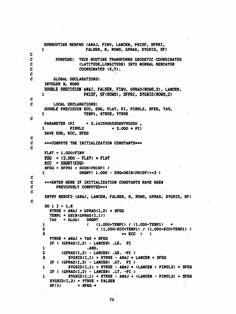
C

SUBROUTINE MERFWD· ( AMAJ, FINV, LAMCEN , PHISF, SFPHI , 1 FALSEN , N , ROWS, GPRAD , XYGRID, .SF)

C PURPOSE : THIS ROUTINE TRANSFORMS GEODETIC COORDINATES C ( LATITUDE , LONGITUDE) INTO NORMAL MERCATOR C COORDINATES ( X , Y ) . C C GLOBAL ·DECLA�ATIONS :

C

INTEGER N, ROWS DOUBLE PRECISION AMAl , rALSEN , rIMV, GPRAD (ROWS , 2) , LAMCEN ,

1 PHISF, SF (ROWS) , SFPHI , XYGRID (ROWS,2)

C LOCAL DECLARATIONS :

C

DOUBLE PRECISION ECC, ESQ , FLAT , PI , PIMUL2 , SFEQ, TAU, 1 TEMP1 , XTRUE , YTRUE ,

PARAMETER (PI : 3 . 141S926S3S897932DO , 1 PIMUL2 : 2 . 0DO • PI )

SAVE ESQ , ECC, SFEQ C C • • • COMPUTE THE INITIALIZATION CONSTANTS ••• C

C

FLAT = 1 . 0DO/FINV �SQ = ( 2 . 0DO. - rLAT) • FLAT ECC = DSQRT (ESQ) SFEQ = SFPHI • DCOS (PHISF) I

1 .

DSQRT ( 1 . 0DO - ESQ.DSIN (PHISF) • • 2 )

C • • • ENTER HERE IF INITIALIZATION CONSTANTS HAVE BEEN C PREVIOUSLY COMPUTED • • -C

C ENTRY MERCF2 (AMAJ , LAMCEN, FALSEN , N , ROWS , �PRAD . XYGRID. SF )

DO 1 I = 1 . N . XTRUE : AMAJ • GPRAD ( I , 2 ) • SFEQ

TEMPI = DSIN ( GPRAD ( I , I » TAU : DLOG ( DSQRT

1 ( ( 1 . 0DO+TEMP1 ) I ( 1 . 0DO-TEMP1 ) -2 ( ( 1 . 0DO-ECC-TEMP1 ) I ( 1 . 0DO+ECC-TEMP1 ) ) 3 • • · ECC ) )

YTRUE = AMAJ - TAU • SFEQ ·IF ( (GPRAD C I , 2 ) - LANCEN) . LE . PI

1 . AND . 2 ( GPRAD ( I , 2 ) - LAMCEN ) . GE . -PI ) 3 XYGRID ( I , l ) = XTRUE - AMAJ • LAMCEN • SFEQ

IF ( (GPRAD C I , 2) - LAMCEN ) · .GT . PI ) 1 XYGRID ( I , 1 ) = XTRUE - AMAJ • ( LAMCEN + PINUL2) • SFEQ

IF ( (GPRAD ( I , 2 ) - LAMCEN ) . LT . -PI ) 1 XYGRID ( I , l ) = XTRUE - AMAJ � ( LAMCEN - PIMUL2) • SFEQ

XYGRID ( I , 2) = · YTRUE + FALSEN SF ( I ) = SFEQ •

76

1

1 2

COIITIIIUE . RETURII

E�D

DSQaT (1 .0DO - ESQ - TEIP1--2) I DeOS( GPR6D ( 1 , 1 ) )

77

C

SUBROUTINE "ERINY (AIIAJ, FINY, ·LAIICEN, PHIS, SFPHI . 1 FALSEN, I, · ROWS, XYGRID, GPRAD, SF)

C .. .

. PURPOSE : THIS ROUTINE TRAIISFORIIS 1I0RlAL IERCATOR .

C COORDIIiATES (X,Y) lITO GEODETIC COORDIIiATES C . (LATITUDE,LOIIGITUDE) . C C GLOBAL DECLARATIOIIS :

C

INTEGER N, ROWS. SLP

. DOUBLE PRECISIOI ·AIIAJ, FALSEN, FIIV, GPRAD CROWS, 2) , LAICEII, 1 PHISF, SF (ROWS) , SFPHI , XYGRID (ROws,2)

C LOCAL DECLARATIORS:

c

C C C

DOUBLE PRECISIOi · ECC, ESQ, FLAT, PHIEST, PI , PIDIV2, PIIIUL2, 1 . SfEQ, " ';KP1 , YTRUE

. PARAIIETER (PI II 3 . 141:5'32653589793200 , 1 PIDIY2 • PI / 2 .0DO " 2 PIIUL2 • PI • 2 . 000 ) colloi 1101 SLP SAYE ECC, ESQ, SFEQ

. . . • • • CONPUTE raE IIITIALIZATIO. COISTAITS • • •

· FLAT • 1 .0DO/FIIIY . . ESQ , • C2 .0DO - FLAT) • FLAT

ECC .. DSQRT CESQ) SFEQ .. SFPHI • DCOS (PHISF) /

1 .

. D5ORT (-· 1 . 0DO � ESQ.OSllI (PHlSF' . . 2 , C C

.• �. EITER HERE · IF IIITIALIZATION CONSTANTS HAVE BEEN

C PREVIOUSLY COMPUTED • • • C

EITRY IIERCI2 ·CAIIAJ, LAIICEI , FALSEN, I, . ROWS, XYGRID, GPRAD, SF) C

DO 2 I = 1 ,1 . YTRUE • XYGRID( I ,2) - FALSEN

e COMPUTE AI .INITIAL APPROXIMATION OF GEODETIC LATITUDE .

C

T = 1 . 0DO / DEXP C YTRUE/ CAIAJ.SFEQ) ) GPRAD C I , 1 ) .. PIDIV2 - 2 . 0DO.DATAN CT)

C PERFORII SUCCESSIVE APPRaXIIATIONS TO OBTAIN THE LATITUDE FOR C THIS POSIT 1011 . . . . e

DO 1 '=1 ,.5 TEIIP1 • ECC.OSIN CGPRAD ( I , 1 » .

C COIIPUTE ·IIEXT APPROXIIATIOIL OF LATITUDE (PHIEST) . PHIEST = PIDIV2 - '

1 2 . 0DO.DATAII C .

T. 2 DSQRT ( · ( ( 1 .0DO-TEIIP1 ) I ( 1 .0DO+TElPl ) )

. . 3

.. ECC ) )

78

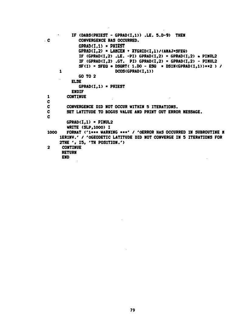
. C

1

IF ( DABS ( PHIEST - GPRAD ( I , 1 » . LE . S . D-9) THEN CONVERGENCE HAS OCCURRED • CPRAD l I . 1 ) = PHI�ST GPRAD ( I , 2) • LAICE. + XYGRID ( I , l ) / (AKAJ·SFEQ) IF (GPRAD ( I , 2 ) . LE . -PI ) GPRAD ( I , 2 ) = GPRAD ( I . 2 ) • PIMUL2 IF ( GPRAD ( I ,2) .GT . PI) GPRAD ( I , 2 ) = GPRAD ( I , 2 ) - PIKUL2 SF ( I ) = SFEQ • DSQRT ( 1 .DO - ESQ • DSIN (GPRAD ( I , 1 » • • 2 ) I

GO TO 2 ELSE

DCOS (GPRAD ( I , 1 »

GPRAD ( I , 1 ) = PRIEST ENDIF

1 CONT�NUE C C CONVERGENCE DID NOT OCCUR WITHIN 5 ITERATIONS . C SET LATITUDE TO BOGUS VALUE AND PRINT OUT ERROR KESSAGE . C

GPRAD ( I , l ) = PIKUL2 WRITE ( SLP , 1000) I

1000 FORMAT ( ' 1 • • • WARNING • • • ' I ' OERROR HAS OCCURRED IN SUBROUTINE I lERINV . ' / ' OGEODETIC LATITUDE DID NOT CONVERGE IN 5 ITERATIONS FOR 2THE " IS, ' TH POSITION . ' )

2 CONTINUE RETURN END

79

C C LOCAL DECLARATIONS :

C

DOU8LE PRECISION A2, A4, A6, A8, 80, 82, 84, 86, C , E3, E4, ES, I E6, E7, ECC3, ESQ, E2SQ, E3SQ, ETASQ, 2 F2, F4, FLAT, L, L2, OMEGA, OMEGAF, PI , 3 PIDIV2, PIKUL2, RN, RREC, S, T, T2, T4, 4 XFAL5E, XTRUE, YFALSE, YTRUE, YVALUE

C THE FOLLOWING ARE TEMPORARY STORAGE VARIABLES : '

C C, E3SQ , L2, T, T2 , T4 . C

PARAMETER (PI = 3 . 141S926S3S897932DO, I PIDIV2 = O . Soo - PI , ' 2 PIMUL2 • 2 . 0DO - PI )

SAVE ESQ, E2SQ, RRE�, YVALUE, BO, B2, B4, B6 C C --- COMPUTE THE INITIALIZATION CONSTANTS ---C

FLAT = 1 . 00 I rIMV ' ESQ • ( 2 . DO - FLAT) • FLAT E2SQ = ESQ I ( 1 . 00 - ESQ) ECC3 • FLAT I ( 2 . DO - FLAT ) E3SQ • ECC3 - - 2 RREC = AMAJ - < 1 . DO - ECC3) - ( i . DO -. E3SQ) •

1 ( I . DO � 2 . 2SDO-E3SQ • 22S . DO-E3SQ--2 I 64 . 00) A2 • ECC3 • ( - 1 . SDO • 9 . 00- E3SQ 116 . DO) A4 • 1S . DO- E3SQ 132 . DO - ( 2 . DO - E3SQ) A6 = -35 . DO • E3SQ • ECC3 I 48 . DO A8 = 31S . DO • E3SQ--2 I S12 . DO BO • 2 . DO - (A2 - 2 . DO-A4 • 3 . DO-A6 -4 . DO-A8 ) B2 • 8 . DO - ( A4 - 4 . DO-A6 • 10 . DO-A8) B4 =

'32 . DO - (A6 - 6 . DO-A8)

B6 = 128 . DO • A8 C • DCOS (PHIFAL) OMEGAF • PHIFAL • C - DSIN ( PHIFAL) •

1 ( 80 '. B2-C--2 • B4-C-.4 • B6-C--6) YVALUE = -SFCEN • OMEGAF • RREC

C C _ . - ENTER HERE IF INITIALIZATION CONSTANTS HAVE BEEN . C PREVIOUSLY COMPUTED • • •

80

C

C

C

EITRY TNFWD2 (ANAJ, LANCEI , FALSEE, FALSEI , SFCEI, N, ROWS, 1 GPRAD, XYGRID, SF)

DO 1 I = 1 , N C = DCOS (GPRAD C I , l »

C IF LATITUDE EQUALS PI/2, DISABLE THE TANGENT FUICTIOI . C SINCE THE INTERNAL REPRESENTATION or LATITUDE IN RADIANS C KAY NOT BE EXACTLY. EQUAL TO THAT or PIDIV2, DISABLE THE C TANGENT FUNCTION IF THE LATITUDE IS WITHIN 1 .0D-I5 OF PIDIV2. C

C

IF ( DABS (GPRAD ( I , l ) - PIDIV2) . LT . 1 . 0D-1S 1 . OR .

2 DABS ( GPRAD ( I � l ) + PIDIV2) . LT . 1 .0D-15 ) THEN T = O . DO

ELSE T = DTAN (GPRAD ( I , l »

ENDIF T2 II T"2 T4 II T2 .. 2 ETASQ II E2SQ • C •• 2 IF ( ( GPRAD ( I ,2) - LANCEN ) . LE . PI

1 . . AND . 2 (GPRAD U , 2), - LANCEN) . GE . -PI ) 3 L II (GPRAD ( I , 2 ) - LAMCEN) • C

IF (' (GPRAD U ,2) ' - LANCEN ) . GT . PI ) 1 L II (GPRAD ( I , 2) - LAMCEN - PIMUL2) • C

IF ( (GPRAD ( I , 2 ) - LANCEN ) . LT . -PI ) 1 L II (GPRAD ( I , 2) - LAMCEN + PIMUL2) • C

C TO AVOID FLOATING POINT UNDERFLOW ERROR ON PERKIN-ELNER 3205 C COMPUTER, REMOVE 4TH AND 6TH ORDER TERMS IN CALCULATION OF ONEGA C WHEN C IS NEAR ZERO (WITHIN A NEIGHBORHOOD OF 1 .0D-l0) . C

IF (C . LT . 1 . 0�-10) THEN

1

1 .

ELSE

ENDIF S RI E3 E4 E5

. E6 : 1

. E7 F2

ONEGA II GPRAD ( I , l ) + C • DSIN (GPRAD ( I , l » • CBO + B2-C--2)

OKEGA II GPRAD ( I , l ) + C • DSIN (GPRAD ( I , l » • (80 + B2-C--2 + B4-C--4 + B6-C--6)

II OKEGA • RREC II AMAJ / DSQRT ( 1 . DO - ESQ-DSIN (GPRAD ( I , l » --2 ) = ( l . DO - T2 + ETASQ) / 6 . DO = ( 5 . DO - T2 + ETASQ - (9 . DO + 4 . DO-ETASQ) ) / 12 . 00 = ( 5 . DO - · 18 . DO-T2 + T4 + ETASQ- ( 14 . DO - 58 . DO-T2» /

120 . DO • ( 61 . DO - 58 . OO-T2 + T4 + ETASQ- (270 . DO - 330 . DO-T2) ) /

360 . DO II (61 .DO - 479 . DO-12 + 179 . DO-T4 - 12-T4 ) / �040 . DO II ( l . DO + ETASQ) / 2 . DO

8 1

F4 • ( 5 . DO - 4 . DO-T2 • ETASQ • ( 9 . DO - 24 . DO-T2) ) I 12 . DO L2 II L--2 XTRUE II SFCEN • RN • L -

1 ( 1 . DO + L2 - ( E3 + L2- ( E5 + E7.L2) ) ) YTRUE • SFCEN • ( S + RN-T-L2 - ( 1 . DO • L2. ( E4 • E6-L2) ) I

1 XFALSE II XTRUE YFALSE II YTRUE • YVALUE . XYGRIDCI , 1 ) = XFALS; • FALS;; XYGRID ( I , 2) • YFALSE • FALSEI

2 . DO )

SF ( I ) II SF9EJ • ( 'l .DO • F2-L2 • ( 1 .00 • F4.L2) )

1 CONTINUE RETURN EID

82

C C C

' C C C

C C

C C C C

SUBROUTINE TIINV (AIAJ, FINV, LAICEN , FALSEE, FALSEN , PHIFAL, 1 SFCEN, N, . ROWS, X'GRID, GPR�D, �F)

PURPOSE : THIS ROUTIN! TRANSFORIS TRANSVERSE IERCATOR ' COORDINATES (X,') INTO GEODETIC COORDINATES

.

(LATITUDE, LONGITUDE) . . . . .

GLOBAL DECLARATIONS : INTEGER N, ROWS DOUBLE PRECISION AIAJ, FALSEE, FALSEN, FIIV, GPRAD (ROWS,2) ,

1 LAICE., PHIFAL, SF CROWS) , SFCE., X'GRID CROWS,2)

LOCAL DECLARATIONS : . DOUBLE PRECISION A2, A4, A6, A8, 80, 82, 84, 86, C,

1 C2, C4 , '06, ·C8, DO, D2, D4, D6, 2 ECCS, ESQ, E2SQ, ESsa, ETASQ, 3 FL.T , G2, G3, G4, G5, G6, G7 , H2, H4, 4 L, LATFP, OIEGA, OIEGAF, PI , PIIUL2, S Q, Q2, RNFP, RREC, S , T, T2, T4� 'VALUE

THE FOLLOWING ARE TEIPORARY STORAGE VARIABLES : C, E3sa, al, T, T2, T4 .

PARAIETER ( PI = 3 . 141592653589793200 , : 1 PIRUL2 • 2 . 0DO • PI ) .

SAVE ESQ, E2SG, RREC, 'VALUE, DO, D2, D4 , . D6 C C · • • • COIPUTE THE INITIALIZATION CONSTANTS • • • C

1

FLAT ESQ E2SQ ECC3 E3SQ . RREC

·A2. A4 A' A8 BO . B2 B4 86 C2 C4 06 C8 DO 02 04

• 1 � 00 1 FIIV • (2.DO � FLAT) • FLAT = ESQ 1 ( l � DO - ESQ) = FLAT 1 ( 2 . 00 - FLAT) = ECCS -- 2 • ARAJ • ( 1 . DO - ECCS) • ( l . DO - E3SQ) •

( 1 . DO • 2 . 25DO.E3SQ .• 225 . DO.E3SQ.-2 1 '4 . 00) • ECes • ( -1 . 500 • 9 . DO.E3SQ/l' . DO) = 15.00 • E3SQ 1 32 . DO - ( 2 . DO - E3sa) • -35 . DO • E3SQ • ECC3 1 48·.DO • 315 � DO • E3SQ.�2 I 512. 00 .

= 2 . 00 • (A2 - 2 .oo-A4 • 3 . DO.A' - 4 . DO-A8) • 8 . 00 • (A4' - 4 . DO-A' • 10 . DO-A8) • 32 . 00 - (A6 - ' . DO.�8) II 128 . DO • A8 • 1 .5DO • ECC3 • ( 1 . DO - 9 . DO-E3SQ/16 .DO) • 21 . 00 • E3SQ 1 1' . DO - 55 . DO • E35Q.-2 I 32 . 00 • 151 . DO • ECC3 • E3SQ I ' 96 . DO

.

• 1097 . DO • E3SQ--2 1 512 . DO • 2 . 00 • (02 - .� . DO.C4 • 3 . DO�06 - 4 . DO-CS) • 8 . 00 • (C4 - 4 . 00-06 . • 10 . DO.C8) • 32 . DO • (06 - 6 . DO-�8)

-

83

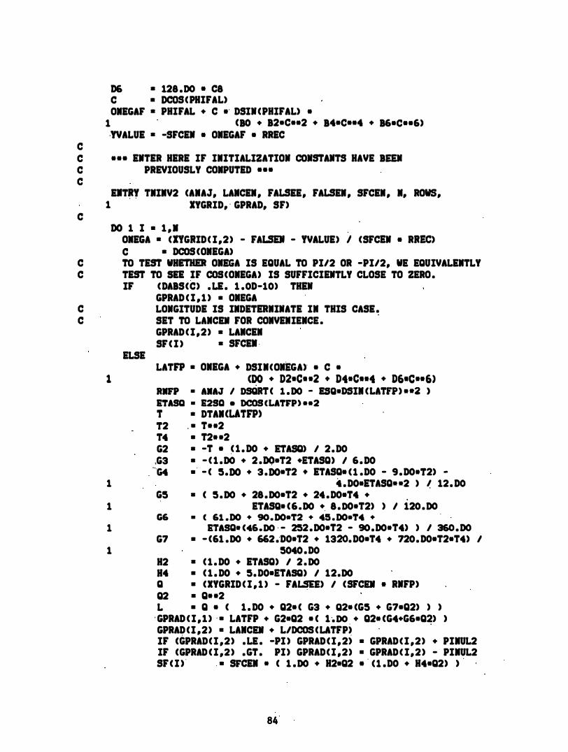
D6 • 128 .00 - C8 C • DCQS( PHIFAL) OIEGAF • PHIFAL • C .' DSIN (PHIFAL) -

1 (10 • 12-C--2 • 14-0--4 • 16-0--6) ,!VALUE • -SFCEN - OIEGAF - RREC

C C --- ENTER HERE IF IIITIALIZATION CONSTANTS HAVE lEEN C PREVIOUSLY COIPUTED ---C

C

E.T�Y TIIIV2 (AIAJ, LAICEI, FALSEE, FALSEI, SFCEI, I, ROWS, 1 XYGRID, ' GPRAD, SF)

DO 1 I • 1 , 1 OIEGA • (IYGRID( I ,2) - FALSEN - !VALUE) I (SFCIN - RREC) C • DCOS (OIEGA)

C TO TEST WHETHER OIEGA IS EQUAL TO PI/2 OR -PI/2, WE EOUIVALEITLY C TEST TO SEE IF cas(OIEGA) IS SUFFICIENTLY CLOSE TO ZERO .

IF (DAIS(C) . LE . 1 .0D-10) THEN GPRAD ( I , l ) • OIEGA

C LONGITUDE IS IIDETERIINATE II THIS CASE . C SET TO LAICEI FOR COIVEIIEICE .

ELSE

GPRAD ( I ,2) • LAICEI SF ( I ) • SFCE. ,

LATFP • OIEGA • DSII(OIEGA), - C -1 (DO • D2-C.-2 • D4-C.-4 • D6.C •• 6)

RIFP • AIAJ I DSQRT ( I . DO - ESQ.DSII (LATFP) • • 2 ) ETASQ • E2S0 • DCQS CLATFP) --2 T • DTAI (LATD) 12 , . T .. 2 T4 • T2 . . 2 G2 • -T - ( l . DO • ETASG) 1 2 . DO

,G3 • - ( l .DO • 2 .DQ-T2 .ETASO) 1 6 . DO , '-'G4 . ' - ( 5.DO • 3 .DO-12 • ETASO- U .DO - 9 . DO.12) -

1 4 . DO-ETASO • • 2 ) � 12. DO G5 • ( 5 . DO • 28 . DO-T2 • 24 . DO-T4 • .

1 ETASQ. ( 6 . DO ., 8 . DO.T2) ) 1 120 . 00 G6 • C 61 .DO • 9O.DO-T2 • 45 . DO-T4 •

1 ETASO. (46.DO ' - 252 . DO.T2 - 9O .DO.T4) ) 1 360 . DO G7 • - (61 . DO • 662 .'DO.T2 • 1320. DO-T4 • 720. DO-T2-T4) 1

1 5040 . DO H2 • ( 1 . DO • ETASO) 1 2 . DO H4 • ( 1 . DO • 5. DO-ETASQ) 1 12.DO o • (XYGRID ( I , 1 ) - FALSE!) 1 (SFCEI • RNFP) 02 • 0 . . 2 L • 0 - ( 1 . DO . 02- ( G3 • 02- (G5 • G7-02) ) )

' GPRAD ( I , U ' . LATFP • G2-02 - ( 1 '. DO , • 02- ('G4.G6-0�) ) GPRAD ( I ,2) • LAICEI • L/DCOS (LATFP) IF (GPRAD( I ,2) . LE . -PI ) GPRAD ( I , 2) • GPRAD C I ,2) • PIIUL2 IF (GPRAD ( I ,2 ) . GT . PI ) GPRAD( I ,2) • GPRAD C I , 2 ) - PIIUL2 SF C I ) , , . SrCEI • ( 1 . DO • H2.02 - ' U .DO • H4-02) ) '

84

ENDIF

1 CONTINUE

RE1'URN

END

85

C

SUBROUTIIE OIFWD (AIAJ, FIIV, PHlCEI, LAICEI , SFCEI , AZICEI , 1 FALSEI, FALSIE, I, ROWS, GPRAD, XYGRID, SF)

C PURPOSE : THIS ROUTIIE TRAISFORIS GEODETIC COORDIIATES · C (LATITU�E� LOIGITUDE) liTO OBLIQUE IERCATOR COORDINATES C ( X , Y) . C C GLOBAL DECLARATIOIS :

C

IITEGER ., ROWS . . DOUILE PRECISION AIAJ, AZICI�, FALSEE, FALSEI, FIRV�

1 GPRAD(ROWS,2) , LAICEI, PHICEI, SF (ROWS) , 2 SFC •• , XYGRID(ROWS,2)

C LOCAL DECLARATIONS :

C

DOUlLE PRECISION A, I, C, CC, D , ECC, ESQ, E2SQ, EXPT, 1 EXPTC, F, FLAT, G , H, J, JC, K , L , LAID, 2 P, S, SC, TEIP, USKEW, ¥SKEW, WSQ

C THE FOLLOWIIG ARE TBIPORARY STORAGE VARIAILES: .C, S, TEIP SAVE ESQ, ECC, I, EXPTC, CC, D, F , G , LAID, H

C C '" CO.PUT! THE IIITIALlZATIOI 001511119. , •• c

C

FLAT ESQ ECC E2SQ S .

C WSQ I . A EXPTC

1 • TEIP SC CC JC D F G LAID H

• ·l . DO I FIIV • (2.DO - FLAT) • FLAT • DSQRT (ESQ) • ESQ I ( l . DO - ESQ) = .DSIII(PHICEI) • DCOS (PHICEN) • 1 . DO - ESQ.S •• 2 • DSQRT ( l . DO . • E2SQ.C • • 4) = I • DSQRT U .DO - ES) I WSQ • DSQRT ( ( l . DO . S) / ( 1 . DO - S) •

( ( 1 . DC) - ECC.S) / ( l . DO • ECC.S) ) •• ECC ) = DSQRT (WSQ) • A = TEIP 1 C = SC • DSQRT ( SC • • 2 - 1 . DO) = (CC - 1 . DO/CC) I 2 . DO • SFCEN • ( A/8) • AIAJ = DSIII (AZICEI) • C I TEIP • DOOS( DASIN(F) ) • LAICEII - DASIII (JC.F/G) I I • SFCEN • A

C • • • EITER HERE IF IIITIALIZATIOI CONSTANTS HAVE IEEI C PREVIOUSLY CO.PUTED • • • C

EITRY O.FWD2 ( AZICEII, FALSD, FALSIE, II , ROWS, GPRAD, 1 XYGRID, SF)

C DO 1 I • 1,1

. 86

L = CGPRAD C I , 2 ) - LAKO) • B S = DSIN CGPRAD C I , l » EXPT = DSQRT ( ( l . DO + S) / ( l .DO -S) -

1 ( ( l . DO - ECC-S) / ( l . DO + ECC-S) ) •• ECC ) P = CC • ( EXPT/EXPTC) --B J = 0 . 5DO • ( P - 1 . DO/P) K = 0 . 5DO - (P + 1 . DO/P ) USKEW = D - DATAN2( (J-G + F-DSINCL» , DCOS (L) ) TEMP = F-J - G-DSIN (L) VSKEW = 0/2 . 00 - OLOG ( (K - TEMP) I (K + TE"P � ) XYGRIO ( I , l ) = USKEW-OSIN (AZICEN ) + VSKEW-OCOS (AZICEN ) + FALSEE XYGRID n , 2) = USKEW.DCOS(AZI"CEN) - VSKEW.DSIN ( AZICEN ) + FALSEN SF U ) = H • DSQRT C l . DO - ESQ-S"2 ) • "DCOS (USKEW/D) I

1 ( DCOS (GPRAD ( I . l » • DCOS (L» 1 CONTINUE

RETURN ENO

87

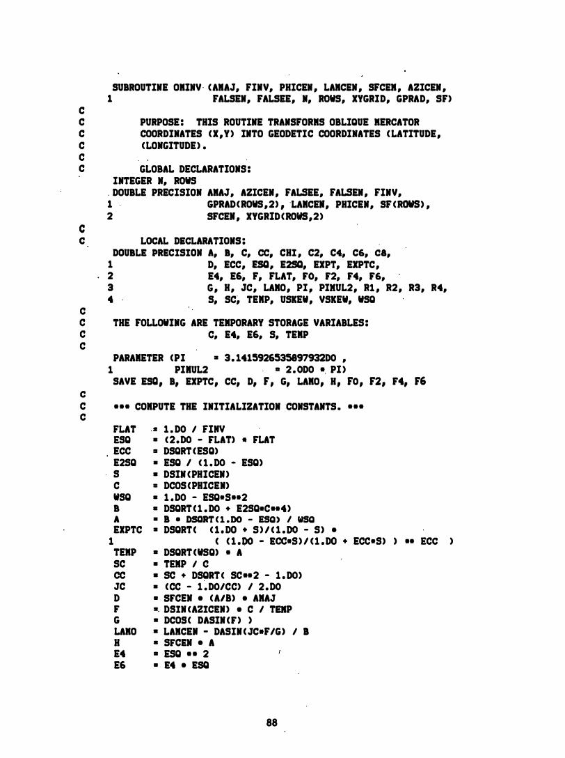
C

SUBROUTINE OIINV · ( AIAJ, FINV, PHICEN , LAICEN , SFCEI , AZICEN , 1 FALSEN, FALSEE, N, ROWS, XYGRID, GPRAD, SF)

C PURPOSE : THIS ROUTINE TRANSFORIS OBLIQUE IERCATOR C COORDINATES ( X , Y ) INTO GEODETIC COORDINATES ( LATITUDE, C (LONGITUDE) . C C GLOBAL DECLARATIONS :

c C

C

INTEGER N, ROWS . DOUBLE PRECISION AIAJ, AZICEN, FALSEE, FALSEN, FINV, 1 GPRAD( ROWS , 2) , ·LAIICEN, PHICEN, SF ( Raws) , 2 SFCEN , XYGRID ( ROWS,2)

LOCAL DECLARATIONS : DOUILE PRECISION A, I, C, ee, CHI , C2, C4, C6, ca,

1 D, ECC, ESQ, E2SQ, EXPT, EXPTC, 2 E4, E6, F, FLAT, ro, r2, r4, r6, 3 G , H , JC, LAIO, PI , PIXUL2, Rl , R2, R3, R4, 4 S, SC� TEIIP, USKEW, VSKEW, WSQ

C THE FOLLOWING ARE TEIPORARY STORAGE VARIABLES : C C, E4, E6, S, TEIIP C

c

PARAIIETER (PI = 3 . 1415926535897932DO , 1 PIIIUL2 . - 2 . 0DO •. PI )

SAVE ESQ , B, EXPTC, CC, D, F, G, LAIIO, H , FO , F2, F4, F6

C • • • COIIPUTE THE INITIALIZATION CONSTANTS . • • • C

FLAT ESQ ECC E2SQ S C WSQ I A EXPTC

1 TEIP SC ee JC D r G LAIO H E4 E6

. D 1 . DO I rIMY • ( 2 . DO - rLAT) • rLAT =- DSQRT (ESQ) • ESQ I ( I . DO - ESQ) • DSIN CPHICEN) = DCOS CPHICEN) • 1 . DO - ESQ.S •• 2 • DSQRT C 1 . DO • E2SQ.C •• 4) • I • DSQRT ( l .DO - ESQ) I WSQ = DSQRTC ( 1 . DO . S ) / ( 1 . oo - S ) •

C C 1 . oo - ECC.S ) / C 1 . DO • ECC.S) ) •• ECC ) - DSQRT CWSQ) • A • TEIP I C • SC • DSQRT ( SC •• 2 - 1 . DO) • (CC - 1 . DO/CC) I 2 . 00 • srCEN • ( All) • AIAJ =. DSIN (AZICEN) • C I TIIP • DCOS( DASIN C r ) ) • LAICEI - DASIN ( JC.F/G) I I • SFCEN • A - ESQ • • 2 • E4 • ESQ

88

C ·

C2 • ESQ/2 . 00 · - ( 1 . 00 • 5 . 00-EsQ/12 . 00 • E4/6 . 00 • 1 1 3 . 00-E6/180 . DO )

C4 = E4 • ( 7 . 00/48 . 00 • 29 . 00-EsQ/240 . D� • 81 1 . DO-E4/11520 . DO ) C6 • E6 • ( 7 . 00/120 . 00 • 81 . DO-ESQ/1120 . DO ) C8 • 4279 . DO - E4--2 1 161280 . DO

ro • 2 . DO • (C2 - 2 . DO-C4 • 3 . DO-C& . - 4 . DO.C8) F2 = 8 . 00 - (C4 - 4 . 00-C6 • 10.00-C8) F4 • 32 . 00 • ( C6 - 6 . DO-C8 ) F6 = 128 . 00 • C8

C • • • EITER HERE IF INITIALIZATIOI COlsTAITS HAVE BEEI C PREVIOUSLY COMPUTED •• -C

C

ENTRY OMIIV2 (AZICEI, FALSEI, FALSEE, N , �OWS, XYGRID, 1 GPRAD, SF)

1

1

1

DO 1 I • 1 , N USKEW

VSKEW

R1 R2 R3 R4 TEMp· EXPT

= eXYGRID ( I , 1 ) - FALSEE) • DsIN (AZICEN ) + (XYGRID ( I , 2) - FALsEN) • DCOs ( AZICEN )

= ( XYGRID ( I , l ) - FALSEE) • DCOS (AZICEN ) (XYGRID ( I ,2) - FALSEN) • DSIN(AZICEN )

• DSINH (VSKEW/D) = DCOSH eVSKEW/D) = DSIN (USKEW/D) = DCOS (UsKEW/D) = Rl .F - R3.,G = ( DSQRT ( (R2 - TEMP) I ( R2 + TEMP) ) 1 CC)

• • ( l . DO/B) • EXPTC CHI = 2 . DO • DATAN ( (EXPT - 1 . 00 ) I (EXPT + 1 . 00) ) S = DSIN (CHI ) C = DCOs (CHI ) GPRAD ( I , 1 ) = CHI + S.C . ( FO + F2.C.-2 • F4-C.-4 +F6-C. -6) GPRAD ( I , 2 ) = LAMO + ( DATAN2 ( (R1-G + R3-F) , R4 ) ) 1 B IF· ( GPRAD C I , 2 ) . LE . -PI ) GPRAD C I , 2 ) = GPRAD C I , 2 ) + PIIIUL2 IF (GPRAD ( I , 2 ) . GT . PI ) GPRAD ( I , 2) = GPRAD ( I , 2) - PIMUL2 SF ( I ) = H • DSQRT ( 1 . DO - EsQ.DsINCGPRAD ( I . l » • • 2) • R4 1

1 ( �COS (GPRAD ( I , 1 » -DCOs « GPRAD ( I , 2 ) - LAMO) • B) ) 1 CONTINUE

RETURN END

89

C

SUBROUTINE LCCFWD (AMAJ , FINV, LAMCEN , PHIN , PHIS, SFN , PHIFAL , .' 1 FALSEN, FALSEE, N , ROWS, GPRAD, XYGRID, SF)

C PURPOSE : THIS ROUTINE TRANSFORMS GEODETIC COORDINATES C (LATITUDE, LONGITUDE) INTO LAMBERT CONFORMAL CONIC C. COORDINATES ( X , Y ) . C C GLOBAL DECLARATIONS :

C

INTEGER N, ROWS DOUBLE PRECISION AMAJ, FALSEE, FALSEN , FINV, GPRAD ( ROWS , 2 ) ,

1 LAMCEN, PHIFAL, PRIN , PHIS, SF (ROWS ) , SFN , 2 XYGRID (ROWS , 2 )

C LOCAL DECLARATIONS :

C

C

DOUBLE PRECISION ECC, ESQ, EXPT, EXPTAU , FLAT, PRICEN , 1 RAD, RADEQ, RADFAL, SCEN , THETA , X , W

SAVE ECC , ESQ, RADEQ, SCEN , RADFAL

C EXPTAU AND W ARE STATEMENT FUNCTIONS USED IN COMPUTATION OF C ZONE CONSTANTS BELOW . THE ARGUMENT OF BOTH FUNCTIONS IS THE C SINE OF THE APPROPRIATE LATITUDE . C

C

( l . DO.X) / ( l . DO-X) • EXPTAU ( X ) = DSQRT ( 1 ( ( l . DO-ECC.X ) · / ( l . DO+ECC.X) ) • • ECC )

= DSQRT ( l . DO - ESQ • X.�2) W ( X )

C ••• COMPUTE THE INITIALIZATION CONSTANTS . • • • C

C

1

1 2

FLAT = 1 . 00 / FINV ESQ = ( 2 . 00 - FLAT) • FLAT ECC = DSQRT ( ESQ)

IF ( PHIN · . EQ . PHIS). - THEN PRICEN = PHIl SCEN = DSIN (PHICEN) RADEQ = SFN • AMAJ • EXPTAU (SCEN ) •• SCEN /

ELSE . SCEN

RADEQ

( W ( SCEM ) • DTAN ( PHICEN ) )

= DLOG ( W ( DSIN ( PHIN» • DCOS ( PHIS) / C W C DSIN CPHIS» • DCOS C PHIN» ) /

DLOG C EXPTAU C DSIN CPHIN» / EXPTAU ( DSIN (PHIS » ) = �FN • AMAJ • DCOS (PHIN) • EXPTAU (DSIN CPHIN» • • SCEN I

1 ENDIF

C W ( DSIN (PHIN» • SCEN ) .

RADFAL = RADEQ / EXPTAU (DSI N ( PHIFAL» • • SCEN C C • • • ENTER HERE IF INITIALIZATION CONSTANTS HAVE BEEN C PREVIOUSLY COMPUTED • • • • C

ENTRY LCCFD2 ( AMAJ, LAMpEN , FALSEN , FALSEE , N , ROWS,

90

1 C

1

DO 1 I = 1 , N RAD THETA XYGRID C I , l > XYGRID C I , 2) SF ( I )

1 CONTINUE RETURN END

GPRAD, XYGRID, SF)

I: RADEQ I EXPTAU ( DSIN (GPRAD C I., l » ) "SCEN I: ( GPRAD ( I ,2) - LAMCEN) • SCEN = FALSEE • RAD • DSIN (THETA) I: RADFAL • FALSEN - RAD • DCOS (THETA) = W( DSIN (GPRAD ( I , l » ) • RAD • SCEN I

C AIAJ • DCOS CGPRAD C I , l » )

9 1

C

SUBROUTINE LCCINV ( AMAJ. FINV. LAMCEN . PHIN . PHIS. SFN . PHIFAL. 1 . FALSEN . FALSEE . N. ROWS. XYGRID. GPRAD. SF)

C PURPOSE : THIS ROUTINE TRANSFORMS LAMBERT CONFORMAL CONIC C. COORDINATES ( X . Y ) INTO GEODETIC COORDINATES (LATITUDE. C LONGITUDE ) . C

C

INTEGER N . ROWS DOUBLE PRECISION AMAJ . FALSEE , FALSEN , FINV, GPRAD (ROWS , 2) ,

1 LAMCEN , PHIFAL. PHIN, PHIS, SF (ROWS) . SFN , 2 XYGRID (ROWS , 2)

C LOCAL DECLARATIONS :

C

C C C c C

C

DOUBLE PRECISION ECC , ESQ. EXPT , EXPTAU . FLAT , Fl . F2 , PHICEN . 1

. PI , PIMUL2, �AD, RADEQ, RADFAL, SCEN , SEST,

2 THETA, X , XTRUE, YPRIME, W

PARAMETER (PI = 3 . 1415926535897932DO , 1 PIMUL2 = 2 . 0DO • PI )

SAVE ECC, ESQ , RADEQ , SCEN , RADFAL ,

EXPTAU AND W ARE STATEMENT FUNCTIONS USED IN COMPUTATION OF ZONE CONSTANTS BELOW . THE ARGUKENT OF BOTH FUNCTIONS IS THE SINE OF THE APPROPRIATE LATITUDE .

( l . DO+X) J ( l . DO-X) • EXPTAU ( X ) = " DSQRT ( 1 ( ( l . DO-ECC.X) I ( l . DO+ECC.X) ) • • ECC )

= DSQRT ( l . DO - ESQ . X • • 2) W ( X )

C • • • COMPUTE THE INITIALIZATION CONSTANTS • • • • C

C

C

1

1 2

FLAT = 1 . DO I FINV ESQ = ( 2 . DO - FLAT) • FLAT ECC = DSQRT (ESQ )

IF (PHIN . EQ . PHIS) THEN

PHICEN = PHIN . SCEN = DSIN (PHICEN) RADEQ = SFN • AMAJ • EXPTAU (SCEN ) •• SCEN I

( W ( SCEN ) • DTAN (PHIC�N ) ) ELSE

SCEN

RADEQ

= DLOG ( W ( DSIN (PHIN» • DCOS (PHIS) I ( W ( DSIN (PHIS» • DCOS (PHIN» ) I

DLOG ( EXPTAU (DSIN (PHIN» I EXPTAU (DSIN (PHIS» )

1 ENDIF

= SFN • AMAJ • DCOS (PHIN) • EXPTAU ( DSI N ( PHIN» •• SCEN I ( W ( DSIN (PHIN » • SCEN )

RADFAL = RADEQ I EXPTAU ( DSIN (PHIFAL» •• SCEN

C ••• ENTER HERE IF INITIALIZATION CONSTANTS HAVE BEEN C PREVIOUSLY COMPUTED . • • • "

92

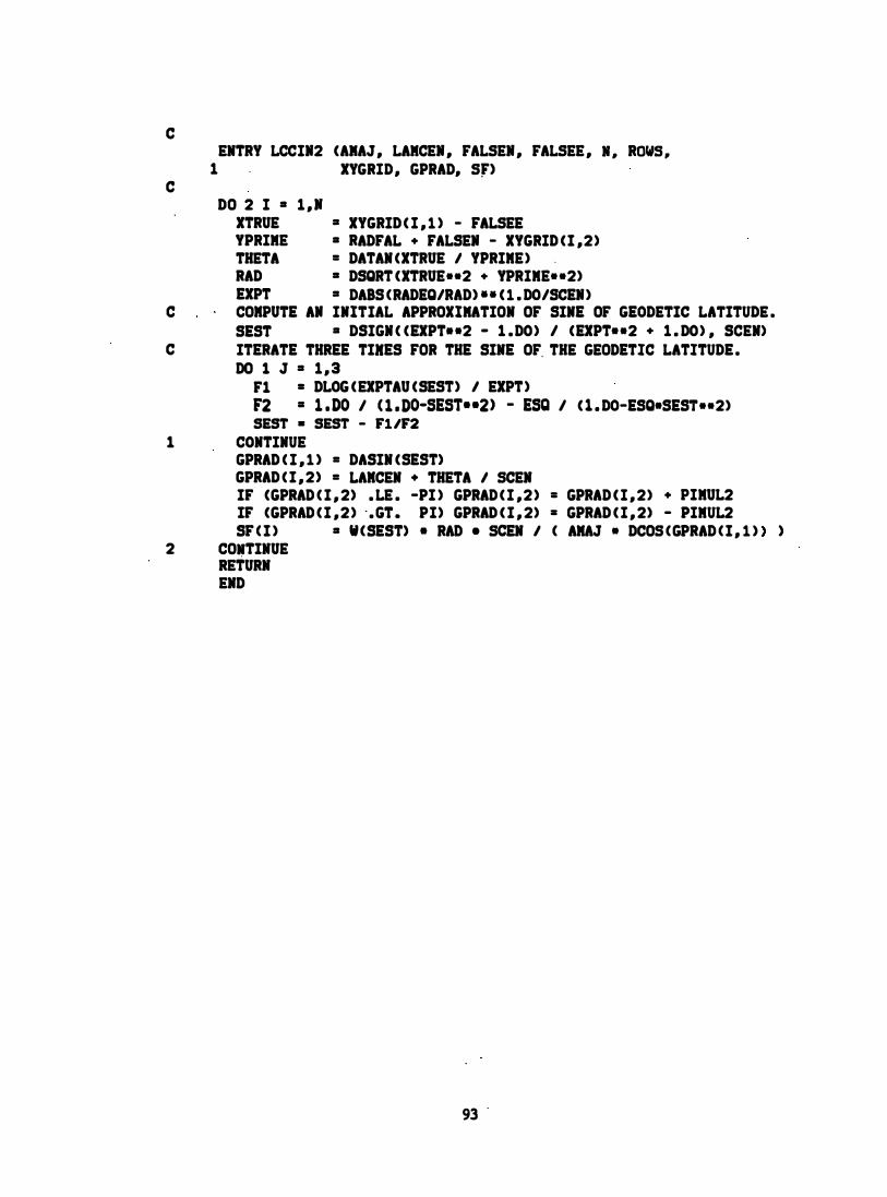
C

C

ENTRY LCCII2 CANAJ , LAMCEI , FALSEI , FALSEE , I , ROWS , 1 XYGRID , GPRAD, S�)

DO 2 I = 1 , 1 XTRUE = XYGRID C I , l ) - FALSEE YPRIME = RADFAL • FALSEI - XYGRID C I ,2) THETA = DATAN CXTRUE I YPRIME) RAD = DSQRT CXTRUE--2 • YPRIME--2) EXPT = DA8S (RADEQ/RAD) .· C l . DO/SCEI)

C COMPUTE AI INITIAL APPROXIMATION OF SINE OF GEODETIC LATITUDE . SEST = DSIGN C CEXPT.-2 - 1 . DO) I CEXPT.-2 • 1 . DO) , SCEN)

C ITERATE THREE TIKES FOR THE SINE OF. THE GEODETIC LATITUDE . DO 1 J = 1 , 3

F1 = DLOG C EXPTAU CSEST) I EXPT) F2 = l i DO I ( 1 I DO-SEST • • 2) - ESQ I C l . DO-ESQ.SEST--2) SEST • SEST - Fl/F2

1 CONTINUE GPRAD C I , l ) = DASIN CSEST) GPRAD C I , 2) = LAMCEN + THETA I SCEN IF CGPRAD C I , 2) . LE . -PI ) GPRAD C I , 2 ) = GPRAD C I , 2) • PIMUL2 IF CGPRAD C I , 2 ) · . GT . PI) GPRAD C I , 2) = GPRAD C I , 2) - PIMUL2 SF ( I ) = W ( SEST) • RAD • SeEN I ( AMAJ • DCOS ( GPRAD ( I , l » )

2 CO�TINUE RETURN END

93 .

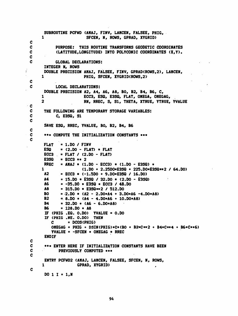
C

SUBROUTINE PCFWD (AMAJ , FINV, LAMCEN , FALSEE , PHIG, . 1 SFCEN , N , ROWS , GPRAD, XYGRID)

C PURPOSE : THIS ROUTINE TRANSFORMS GEODETIC COORDINATES C ( LATITUDE, LONGITUDE) INTO POLYCONIC COORDINATES ( X, Y ) . C C GLOBAL DECLARATIONS :

C

INTEGER N, ROWS DOUBLE PRECISION AMAJ, FA"LSEE , FINV, GPRAD (ROWS , 2) , LAMCEN ,

1 PHIG, SFCEN, XYGRID(ROWS , 2 ) ·

C LOCAL DECLARATIONS :

· C

DOU8LE PRECISION A2, A4, A6, A8, 80, 82, 84, 86, C, 1 ECC3, ESO, E35O, FLAT, OMEGA, OMEGAG, 2 RN, RREC, S, 51 , THETA, XTRUE, YTRUE, YVALUE

C THE FOLLOWING ARE TEMPORARY STORAGE VARIA8LES : C C, E3S0 , 51 C

SAVE ESO , RREC, YVALUE, BO, 82, 84, 86 C C • • • COMPUTE THE INITIALIZATION CONSTANTS • • • C

C

FLAT = 1 . 00 I FINV ESO = ( 2 . DO - FLAT) • FLAT ECC3 = FLAT I (2 . 00 - FLAT) E3S0 = ECC3 •• 2 RREC = AMAJ • ( 1 . 00 - ECC3) • ( 1 . 00 - E3SQ) •

1 ( 1 . 00 + 2 . 25DO.E3SQ + 225 . 00.E3S0 •• 2 I 64 . 00) A2 = ECC3 • ( - 1 . 500 + 9 . DO.E3SQ I 16 . 00) A4 = 15 . 00 • E3SQ I 32 . DO • ( 2 . 00 - E3SQ) A6 = -35 . 00 • E3SQ • ECC3 I 48 . DO A8 = 315 . DO • E3S0 •• 2 I 512 . 00 80 = :·2 . 00 • ( A2 - 2 . DO.A4 + 3 . DO.A6 -4 . DO.A8) 82 .=. 8 . 00 • (A4 - 4 . DO.A6 + 10 . DO.A8) B4 = 32 . 00 • ( A6 - 6 . DO.A8) 86 = 128 . 00 • A8 IF (PHIG . EO . 0 . 00) YVALUE = 0 . 00 IF ( PHIG . NE . O . DO ) THEN

C = DCOS (PHIG) OMEGAG = PHIG + DSIN (PHIG) .C. (BO + B2-C •• 2 + B4-C •• 4 + B6.C.-6) YVALUE = -SFCEN • OMEGAG • RREC

ENDIF '

C •• • ENTER HERE IF INITIALIZ�TION CONSTANTS HAVE 8EEN C PREVIOUSLY COMPUTED • • • C

ENTRY PCFWD2 ( AMAJ, LAMCEN, FALSEE, SFCEN, N , ROWS, 1 GPRAD, XYGRID)

C DO 1 I = 1 , N

94

C • DC05 CGPRAD C I , 1 » 51 • DSINCGPRAD C I , 1 » THETA = CGPRAD C I , 2) - LAMCEN) • S1 OMEGA • GPRAD ( I , 1 ) • S1 • C • ( BO • B2.C •• 2 • B4.C •• 4 • B6.C •• 6 ) S = OMEGA • RREC RN � AMAJ I DSQRT C 1 . DO - ESQ . S1 • • 2) IF CGPRAD C I , l ) . EO . O . DO) THEN

XTRUE = SFCEN • AMAJ • CGPRAD C I , 2) - LAMCEN> YTRUi == O . DO

ELSE IF (THETA . EQ . O . DO) THEN

XTRUE = O . DO

ELSE YTRUE = SFCEN • S

XTRUE = SFCEN • ( RN • DSIN(THETA ) I DTAN (GPRAD ( I , l » ) YTRUE = SFCEN •

1 "( S ". RN" • < 1 . DO - DCOS (THETA» I DTAN (GPRAD U , U ) ) ENDIF

ENDIF XYGRID ( I , 1 ) = XTRUE • FALSEE XYGRID C I , 2) = YTRUE • YVALUE

1 CONTINUE RETURN END

95

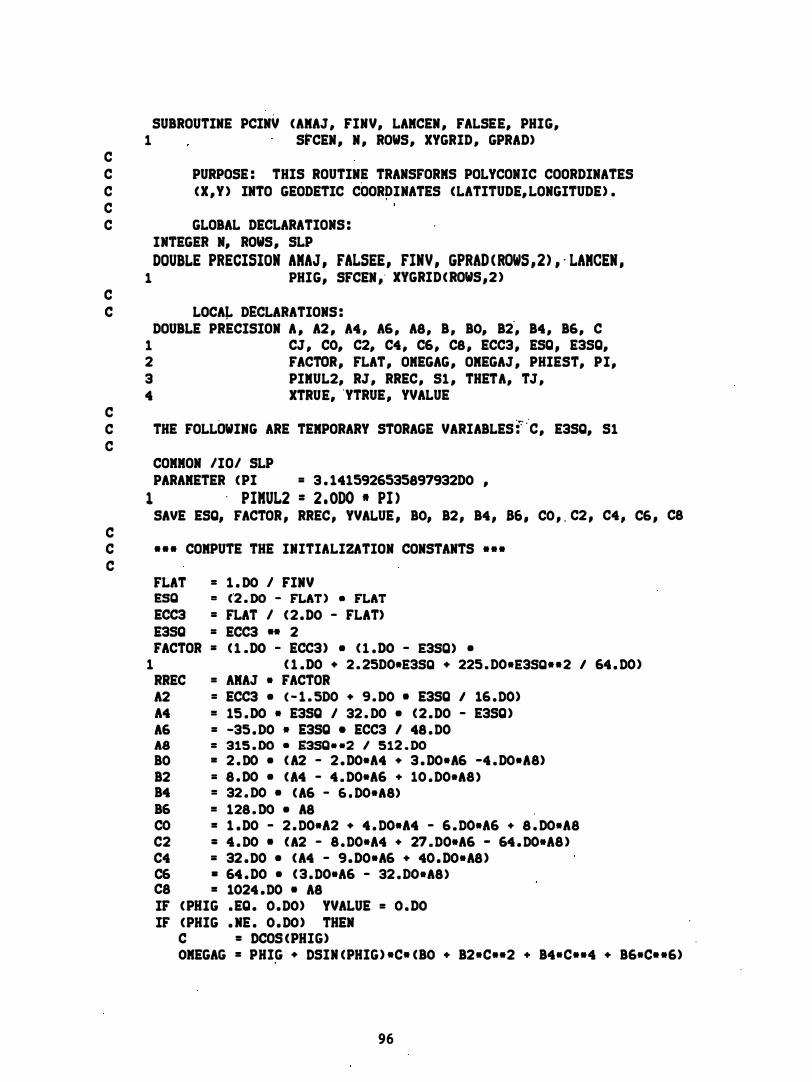
C

SUBROUTINE PCINV (AMAJ , FINV, LAMCEN , FALSEE, PHIG, 1 StCEN, N , ROWS, XYGRID , GPRAD)

C PURPOSE : THIS ROUTINE TRANSFORMS POLYCONIC COORDINATES C ( X , Y ) INTO GEODETIC COORPINATES (LATITUDE, LONGITUDE) . C C GLOBAL DECLARATIONS :

C

INTEGER N, ROWS, SLP DOUBLE PRECISION AMAJ, FALSEE, FINV , GPRAD ( ROWS , 2) , · LAMCEN ,

1 PHIG, SFCEN ," XYGRID ( ROWS , 2 )

C LOCA� DECLARATIONS :

C

DOUBLE PRECISION A , A2 , A4 , A6 , AS, B , BO, B2", B4 , B6, C 1 CJ , CO, C2, C4 , C6, CS , ECC3, ESQ, E3SQ, 2 FACTOR, FLAT, OMEGAG, OMEGAJ , PHIEST, PI, 3 PIMUL2, RJ , RREC, Sl , THETA, TJ , 4 XTRUE, "YTRUE, YVALUE

C THE FOLLOWING ARE TEMPORARY STORAGE VARIABLES f :c, E3SQ, Sl C

C

COMMON IIOI SLP PARAMETER ( PI = 3 . 1415926535S97932DO ,

1 " PI"UL2 = 2 . 0DO • PI ) SAVE ESQ, FACTOR , RREC, YVALUE , BO, B2, B4 , 86 , CO , . C2 , C4 , C6 , C8

C • • • COMPUTE THE INITIALIZATION CONSTANTS ---C

FLAT = 1 . DO I FINV ESQ = C"2 . DO - FLAT) • FLAT

ECC3 = FLAT I ( 2 . DO - FLAT) E3SQ = ECC3 -- 2 FACTOR = ( l . DO - ECC3) • ( l . DO - E3SQ) •

1 ( l . DO • 2 . 2500-E3SQ • 225 . 00-E3SQ--2 I 64 . 00) RREC = AMAJ - FACTOR A2 = ECC3 • ( - 1 . 500 • 9 . 00 • E3SQ I 16 . 00) A4 = lS . DO - E3SQ I 32 . 00 • ( 2 . DO - E3SQ) A6 = -35 . 00 - E3SQ • ECC3 I 4S . 00 A8 = 315 . 00 • E3SQ- -2 I 512 . DO

BO = 2 . 00 • ( A2 - 2 . DO-A4 • 3 . DO-A6 -4 . DO-A8) B2 = S . OO • ( A4 - 4 . 00-A6 • 10 . 00-AS )

B4 = 32 . 00 • ( A6 - 6 . 00-A8)

B6 = 128 . DO • AS CO = 1 . DO - 2 . 00-A2 • 4 . 00-A4 - 6 . 00-A6 + S . OO-AS C2 = 4 . 00 • ( A2 - 8 . 00-A4 + 27 . 00-A6 - 64 . 00-A8 ) C4 = 32 . 00 • ( A4 - 9 . DO-A6 • 40 . DO-AS ) C6 • 64 . DO • ( 3 . 00-A6 - 32 . 00-A8)

CS = 1024 . 00 • AS IF ( PHIG . EQ . O . DO) YVALUE = O . DO IF (PHIG . NE . O . DO) THEN

C = OCOS (PHIG) OMEGAG = PHIG • OSIN (PHIG) .C. (BO • B2-C--2 • B4-C--4 • B6-C- -6)

96

C

YVALUE = -SFCEN • OMEGAG '- RREC ENDI�

C --- ENTER HERE IF INITIALIZATION CONSTANTS HAVE BEEN C PREVIOUSLY COMPUTED ---C

C

ENTRY PCINV2 (AMAJ, . LAMCEN , FALSEE , SFCEN , N, ROWS , 1 XYGRID, GPRAD)

DO 3 I = 1 , N XTRUE = XYGRID ( I , l ) - FALSEE YTRUE = XYGRID ( I , 2) - YVALUE IF (YTRUE . EQ . O.DO) THEN

GPRAD ( I , 1 ) = O . DO GPRAD ( I , 2 ) = LAMCEN + XTRUE J ( SFCEN • AKAJ )

ELSE A = YTRUE / (SFCEN • AMAJ) B = ( XTRUE / (SFCEN-AMAJ ) ) - -2 + A- -2

C SET FIRST APPROXIMATION OF GEODETIC LATITUDE . GPRAD ( I , l ) = A

C C PERFORM SUCCESSIVE APPROXIMATIONS TO OBTAIN THE LATITUDE C FOR THIS POSITION . c

C

C

1

C C C

DO 1 J= 1 , 5 C = DCOS (GPRAD ( I , l » S1 .= DSIN (GPRAD ( I , 1 » CJ = DSQRT ( l . DO - ESQ-Sl --2) • DTAN (GPRAD C I , l » OKEGAJ = GPRAD ( I , 1 ) +

1 Sl-C - ( BO + B2-C--2 + B4-C- -4 + B6-C- .6)

1

1 2 3

1

RJ = OMEGAJ • FACTOR TJ = FACTOR •

( CO + C2-C--2 + C4-C- -4 + C6.C--6 + CS-C--S) COMPUTE NEXT APPROXIMATION OF LATITUDE (PHIEST) . PHIEST = GPRAD ( I , l ) -

( A- (CJ-RJ + 1 . DO) - RJ - CJ- (RJ- -2 + B ) /2 . DO ) / ( 2 . DO-ESQ-SI -C- (RJ--2 + B - 2 . DO-RJ-A) / ( 4 . DO-CJ) . . + (A - RJ) - (CJ-TJ - 1 . DO/ C S1-C» - TJ )

IF (DABS (PHIEST - GPRAD ( I , 1 » . LT . 5 . 0-9) THEN CONVERGENCE HAS OCCURRED . GPRAD ( I , 1 ) = PHIEST GPRAD ( I , 2 ) = LANCEN + DASIN ( CJ-XTRUE / ( SFCEN-AMAJ) ) /

DSIN ( PHIEST) GO TO 2

ELSE GPRAD ( I , l ) = PHIEST

ENDIF CONTINUE

CONVERGENCE DID NOT OCCUR WITHIN 5 ITERATIONS . SET LATITUDE TO BOGUS VALUE AND PRINT OUT ERROR NESSAGE .

97

C GPRAD ( I , 1 ) = 8 . DO ,. DATAN C 1 . DO ) WRITE ( SLP , 1000) I

1000 FORKAT C ' O • • • WARNING • • • ' I ' OERROR HAS OCCURRED IN SUBROUTIN IE PCINV . ' I ' OGEODETIC LATITUDE DID NOT CONVERGE IN 5 ITERATIONS F 20R THE " IS, ' TH POSITION . ' )

ENDIF 2 IF CGPRAD C I , 2 ) . LE . -pi ) GPRAD ( I , 2 ) = GPRAD C I , 2) • PIKUL2

IF (GPRAD C I , 2 ) . GT . PI > GPRAD C I , 2) '= GPRAD C I , 2 ) - PIKUL2 3 CONTINUE

'RETURN END

98

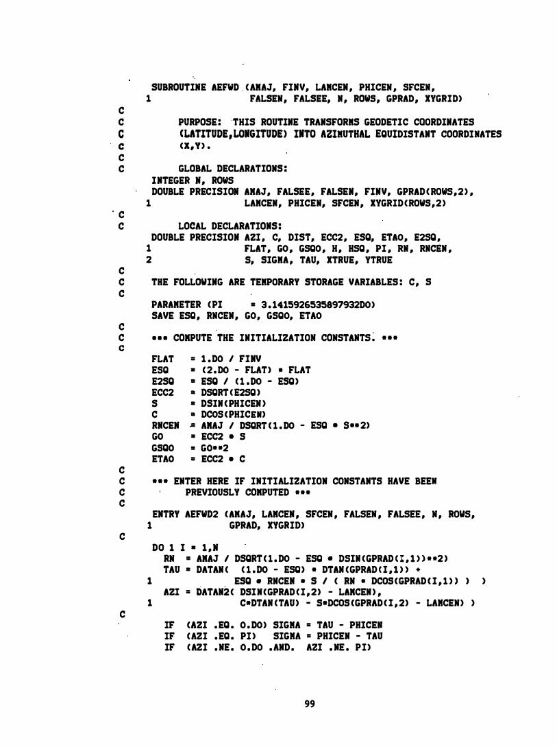
C

SUBROUTINE AEFWD . ( AMAJ, FINV, LAMCEN , PHICEN , SFCEN , 1 FALSEN, FALSEE, N , ROWS, GPRAD, XYGRID)

C PURPOSE : ·THIS ROUTINE TRANSFORMS GEODETIC CaORDINATES C (LATITUDE, LONGITUDE) INTO AZIMUTHAL EQUIDISTANT COORDINATES c (X,V) . C C GLOBAL DECLARATIONS :

· C

INTEGER N, ROWS DOUBLE PRECISION AMAJ, FALSEE, FALSEN, FINV, GPRAD ( ROWS , 2 ) ,

1 LAMCEN, PHICEN, SFCEN, XYGRID (ROWS , 2 )

C LOCAL DECLARATIONS :

C

DOUBLE PRECISION AZI , C, DIST, ECC2, ESQ, ETAO, E2SQ , 1 FLAT, GO , GSQO , H , HSQ , PI , RN , RNCEN , 2 5, SIGMA , TAU, XTRUE, YTRUE

C THE FOLLOWING ARE TEMPORARY STORAGE VARIABLES : C , S C

C

PARAMETER ( PI = 3 . 1415926535897932DO) SAVE ESQ, RNCEN, GO, GSQO, ETAO

C • • • COIPUTE THE INITIALIZATION CONSTANTS : • • • c

C

FLAT ESQ E2SQ ECC2 S C RNCEN GO GSQO ETAO

= 1 . DO I FINV = ( 2 . DO - FLAT) • FLAT = ESQ I ( l . DO - ESQ) II DSQRT C E2SQ ) = DSIN C PHICEN ) II DCOS (PHICEN) � AMAJ I DSQRT ( l . DO - ESQ . 5 •• 2) = ECC2 • S = GO· ·2 = ECC2 • C

C • • • ENTER HERE IF INITIALIZATION CONSTANTS HAVE BEEN C PREVIOUSLY COIPUTED • • • C

C

C

ENTRY AEFWD2 (AIAJ, LAICEN , SFCEN , FALSEN , FALSEE , N , ROWS, 1 GPRAD, XYGRID)

DO 1 I • 1 , N RN = AIAJ I DSQRT ( l . DO - ESQ • DSIN (GPRAD C I , 1 » • • 2 ) TAU = DATAN ( ( l . DO - ESQ) • DTAN (GPRAD C I , 1 » +

1 ESQ . RNCEN • S I ( RN • DCOS (GPRAD ( I , l » ) ) AZI = DATAN2 ( DSI N (GPRAD ( I , 2) - LAICEN ) ,

1 C.DTAN (TAU) - S.DCOS (GPRAD ( I , 2) - LAMCEN) )

IF (&ZI . EQ . O . DO) SIGMA = TAU - PHICEM IF (AZI . EQ . PI ) SIGMA = PHICEN - TAU IF (AZI . NE . O . DO . AND . AZI . NE . P I )

99

C 1 SIGMA = DASIN ( DSIN( GPRAD ( I , 2) -LAMCEN) • DCOS (TAU) /DSIN CAZI »

H = ETAO • DCOS (AZI ) HSQ • H • • 2

DIST = RRCER • SIGMA • 1 ( 1 . DO - SIGMA • • 2 • HSQ . • . ( l . DO - HSQ) 1 6 . DO • 2 ( SIGMA • • 3 I a . DO) • GO • H • ( 1 . D() - 2 . DO.HSQ) • 3 (SIGMA • • 4 I 120 . DO) • (Hsa • ( 4 . DO - 7 . DO.HSQ) 4 - 3 . DO • GSQO • ( 1 . D() � 7 . DO.HSQ» S (SIGMA • • S I 48 . DO ) • GO • H )

XTRUE = SFCER • DIST • DSIN (AZI ) 'TRUE = SFCER • DIST • DCOS (AZI ) X'GRID ( I , l ) • XTRUE + FALSEE XYGRID ( I , 2 ) = YTRUE + FALSE.

1 CONTINUE RETURN END

100

C

SUBROUTINE AEINV (AMAJ , FINV, LAMCEN , PHICEN , SFCEN , 1 FALSEN , FALSEE, N, ROWS, XYGRID, GPRAD)

C PURPOSE : THIS ROUTINE TRANSFORMS AZIMUTHAL EQUIDISTANT C COORDINATES ( X , Y ) INTO GEODETIC COORDINATES CLATITUDE, C LONGITUDE ) . C C GLOBAL DECLARATIONS :

C

INTEGER N , ROWS DOUBLE PRECISION AMAJ , FALSEE , FALSEN , rIMV , GPRAD C ROWS , 2 ) ,

1 LAMCEN , PHICEN, srCEN , XYGRIDC ROWS, 2 )

C LOCAL DECLARATIONS :

C

DOUBLE P�ECISION A, A2I , B , C, CA , D, DIST, E , ESQ, ETASQO , . E2SQ, 1 F , FLAT , PI , PIMUL2, RN , RNCEN , S, TAU , XTRUE, 2 YTRUE

C THE FOLLOWING ARE TEMPORARY STORAGE VARIABLES : C, CA , S C

C

PARAMETER CPI = 3 . 1415926535897932DO, 1 PIMUL2 = 2 . DO • PI )

SAVE ESQ , E2SQ , RNCEN , ETASQO

·C • • • COMPUTE THE INITIALIZATION CONSTANTS • • • • C

C

FLAT ESQ E2SQ S C RNCEN

= 1 . DO I FINV = C 2 . DO - FLAT) • FLAT = ESQ I C l . DO - ESQ ) = DSINC PHICEN ) = DCOS (PHICEN ) = AMAJ I DSQRT ( l . DO - ESQ . S • • 2>

ETASQO = E2SQ • C •• 2

C • • • ENTER HERE IF INITIALIZATION CONSTANTS HAVE BEEN C PREVIOUSLY COMPUTED • • • C

C

ENTRY AEINV2 (AMAJ , LAMCEN , SFCEN , FALSEN , FALSEE, N, ROWS, 1 XYGRID, GPRAD >

DO 1 I = 1 , N XTRUE = XYGRID ( I , l ) - FALSEE YTRUE = XYGRID C I , 2 ) - FALSEN DIST = DSQRT C XTRUE • • 2 + YTRUE�.2 ) I SFCEN AZI = DATAN2 C XTRUE, YTRUE> CA = DCOS C AZI ) A = ETASQO • CA •• 2 B = 3 . DO • E2SQ • ( l . DO + A ) • S • C • CA D = DIST I RNCEN E = D + A • ( 1 . 00 - A ) • 0 • • 3 I 6 . 00 -

1 B • ( 1 . 00 - 3 . DO.A) • D • • 4 I 24 . DO F = 1 . DO + A • ( E • • 2 I 2 . DO ) - B • (E • • 3 I 6 . DO )

101

TAU = DASII CS • DCOS CE) + C • DSII CE) • CA ) GPRAD ( I , 1 ) = DATAI ( ( DTAI ( TAU) - ESQ . F • S I DCOS ( TAU» I

2 ( l . DO - ESQ) ) GPRAD ( I , 2) = LAMCEI + DASII ( DSII (AZI) • DSII ( E ) I DCOS C TAU) ) IF (GPRAD ( I , 2 ) . LE . -PI ) GPRAD ( I ,2) = GPRAD ( I , 2 ) + PIMUL2 .

IF (GPRAD C I , 2) . GT . PI ) GPRAD ( I ,2) = GPRAD C I ,2) - PIMUL2 1 COITIIUE

RETURN END

1 02

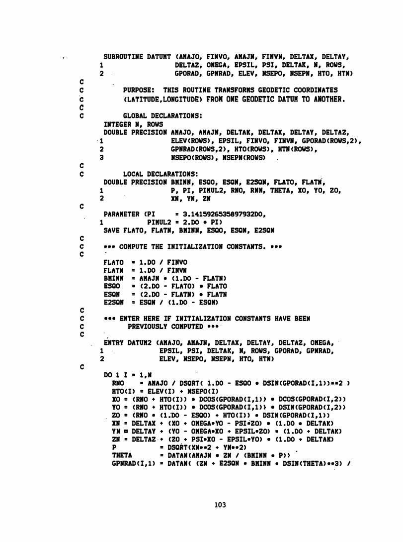
C

SUBROUTINE DATUMT ( AMAJO� FINVO� AMAJN� FINVN� DELTAX � DELTAY � 1 DELTAZ, OMEGA, EPSIL, PSI , DELTAK , N , ROWS , 2 GPORAD, GPNRAD, ELEV, NSEPO, NSEPN , HTO , HTN )

C PURPOSE : THIS ROUTINE TRANSFORMS GEODETIC COORDINATES C ( LATITUDE . LONGITUDE) FROM ONE GEODETIC DATUM TO ANOTHER . C C GLOBAL DECLARATIONS :

C

INTEGER N , ROWS DOUBLE PRECISION AMAJO, AMAJN, DELTAK, DELTAX, DELTAY , DELTAZ,

' 1 ELEV (ROWS) , EPSIL, FINVO, FINVN , GPORAD (ROWS, 2 ) , 2 GPNRAD (ROWS , 2 ) , HTO CROWS ) , HTN (ROWS ) , 3 NSEPO ( ROWS) , NSEPN CROWS)

C LOCAL DECLARATIONS :

C

DOUBLE PRECISION BMINN, ESQO, ESQN, E2SQN, FLATO , FLATH, 1 P , PI , PIMUL2, RNO� RNN, THETA , XO, YO, ZO, 2 XN , YN , ZN

PARAMETER (PI = 3 . 141592653589793200 , 1 PIMUL2 = 2 . 00 • PI )

SAVE FLATO , FLATN, BMINN, ESQO , ESQN , E2SQN C C • • • COMPUTE THE INITIALIZATION CONSTANTS . • • • C

C

FLATO FLATN BMINN ESQO ESQN E2SQN

= 1 . DO I FINVO = 1 . 00 I FINVN = AMAJN • ( 1 . 00 - FLATN ) = ( 2 . 00 - FLATO) • FLATO = ( 2 . DO - FLATN ) • FLATN = ESQN I ( 1 . 00 - ESQN)

C • • • ENTER HERE IF INITIALIZATION CONSTANTS HAVE BEEN C PREVIOUSLY COMPUTED • • • . C

C

ENTRY DATUM2 ( AMAJO, AMAJN , DELTAX , DELTAY � DELTAZ , OKEGA , 1 EPSIL, PSI , DELTAk, N, ROWS, GPORAD, GPNRAD, 2 ELEV , NSEPO , NSEPN , HTO, HTN )

DO 1 I = 1 , N . RNO = AMAJO I DSQRT ( 1 . 00 - ESQO • DSIN (GPORAD ( I � 1 » • • 2 ) HTO ( I ) = ELEV ( I ) + NSEPO ( I ) XO = ( RNO + KTO ( Z » • DCOS (GPORAD ( I , l » • DCOS (GPORAD ( I , 2 » YO = (RNO + HTO ( I » • DCOS (GPORAD ( I , l » • DSIN (GPORAD ( I , 2 » 20 = (RNO • ( 1 :00 - ESQO) + KTO ( 1 » • DSIN (GPORAD ( l , l » XN = DELTAX + ( XO + OMEGA.YO - PSI -20) • ( 1 . 00 • DELTAK) YN a DELTAY + (YO - OMEGA-XO + EPSIL.20) • ( 1 . 00 + DELTAK ) 2N = DELTA2 · + (ZO + PSI-XO - EPSIL.YO) • ( 1 . 00 + DELTAK) P = DSQRT ( XN • • 2 + YN-.2) THETA = DATAN ( AMAJN • ZN I (BMINN • P» GPNRAD ( I , l ) = DATAN ( (2N + E2SQN • BMINN • DSIN (THETA) • • 3 ) I

103

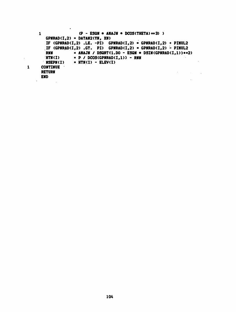
1 CP - ESQN • AIAJN • DCOS CTHETA) •• 3) ) GPNRAD C I ,2 ) = DATAN2 CYI , XI ) , IF CGPNRAD C I , 2) . LE . -PI ) GPNRAD C I , 2) . GPNRAD C I , 2) + PIIUL2

, IF CGPNR�D C I , 2 ) . GT . PI ) GPIRAD C I , 2 ) . GPIRAD C I , 2 ) � PIIUL2 RNN = AIAJN I DSQRT C 1 . DO - ESQN • DSIN CGPNRAD C I , 1 » • • 2 )

' HTI ( I ) = P I DCOS (GPIRAD ( I , l » - RIN NSEPN ( I ) = HTN ( l ) - ELEV ( I )

1 CONTINUE RETURN END

104

APPENDIX E. -- TEST POINTS

Test points are incl uded in thi s appendfx to provfde a standard against whi ch to compare resul ts in the event the subroutines are somed� revi sed . Parameters and coordinates have been chosen not as those that woul d be typical ly found in practice , but rather , those that thoroughly exerci se the transformations . Whole-degree l atitudes and longi tudes are transformed to XiS and y ' s . which are then transformed back to latitudes and longitudes . The " Round Trip Errorn i s the difference in degrees between the starting and endi ng coordi nates . Both the pl anar coordi nates and round tri p error shou l d be used to check the resul ts of future revis ions .

105

NORMAL MERCATOR TRANSFORMATION TEST POINT.S ON GRS 80, ELLIPSOID . SEMIMAJOR AXIS = 6378137 . RECIPROCAL OF FLATTENING = 298 . 257222101

PROJECTION PARAMETERS : CENTRAL MERIDIAN = . O . DEGREES REFERENCE LATITUDE FOR SCALE FACTOR = O . SCALE FACTOR AT REFERENCE LATITUDE = 1 / 1 FALSE NORTHING = 0 . 0

ORIGINAL POSITION LAT LON �"� . O .

o . -60 . O . 120 . O . -180 . O . 240 .

TRANSFORMED POSITION X Y

O . OOOOOOOOOOOOE+OO O·. OOOOOOOOOOOOE+OO· - . 667916944760E+07 O . OOOOOOOOOOOOE+OO 0 . 133583388952E+08 O . OOOOOOOOOOOOE+OO - . 200375083428E+08 O . OOOOOOOOOOOOE+OO - . 133583388952E+08 O . OOOOOOOOOOOOE+OO

PROJECTION PARAMETERS : CENTRAL MERIDIAN = 90 . DEGREES REFERENCE LATITUDE FOR SCALE FACTOR = 25 .

. . SCALE FACTOR AT REFERENCE LATITUDE = 1 / 100 FALSE NORTHING = -25000 . 0

ORICINAl POSITION LAT LON 29 . O . 29 . -60 . 29.. 120 . 29 . -180 . 29 . 240 . ·

TRANSFORMED POSITION X Y

- . 908550812557E.05 0 . 542423039994£.04 - . 151425135426E.06 0 . 542423039994E+04 0 . 302850270852E+05 0 . 542423039994E+04 0 . 908550812557E+05 0 . 542423039994E+04 0 . 151425135426E+06 0 . 542423039994E+04

PROJECTION PARAMETERS : CENTRAL MERIDIAN = - 180 . DEGREES REFERENCE LATITUDE FOR SCALE ' FACTOR = 50 . SCALE FACTOR AT REFERENCE LATITUDE = 1 / 10000 FALSE NORTHING = 500 . 0

ORIGINAL POSITION

LAT LON -58 . O. -58 . -60 . -58 . 120 . -58 . -180 . -58 . 240 .

TRANSFORRED POSITION

X Y 0 . 129052356510E+04 - . 10802351 1948E+02 0 . 860349043400E+03 - . 108023511948E+02 - . 430174521700E+03 - . 10802351 1948E+02 O . OOOOOOOOOOOOE+OO - . 10802351 1·948E+02 0 . 430174521700E+03 - . 108023511948E+02

PROJECTION PARAMETERS : CENTRAL MERIDIAN = 270 . DEGREES REFERENCE LATITUDE FOR SCALE FACTOR = 75 . SCALE FACTOR AT REFERENCE LATITUDE = 1/1000000 FALSE NORTHING = -7 . 5

106

ROUND TRIP ERROR LAT LON

- . 12722£-13 0 . 00000£+00 - . 12722E-13 0 . 35527E- 14 - . 12722E-13 0 . 35527£- 14 - . 12722E-13 O . OOOOOE+OO - . 12722E-13 O . OOOOOE+OO

ROUND TRIP ERROR LAT LON

0 . 11278£-09 0 . 00000£+00 0 . 1 1278E-09 0 . 35527E- 14 0 . 1 1278E-09 0 . 35527E-14 0 . 1 1278E-09 O . ooOOOE+OO 0 . 1 1278E-09 O . OOOOOE+OO

ROUND TRIP ERROR LAT LON

- . 22240E-11 O . OOOOOE+OO - . 22240E-l1 0 . 35527E-14 - . 22240E-l1 0 . 35527E- 14 - . 22240E-11 O . OOOOOE+OO - . 22240E-11 O . OOOOOE+oo

ORIGINAL POSITION LAT LON 81 . O . 87 . -60. 81 . 120 . 87 . -180 . 81 . 240 .

TRANSFORIED POSITION X Y

0 . 260118052292£+01 - . 141919489501£+01 0 . 861060114308E+00 - . 147919489501E+Ol - .433530087154E+Ol - . 141919489501E+01 - . 260118052292E+Ol - . 147919489501£+01 - .867060174308E+00 - . 147919489501E+Ol

107

ROUND TRIP ERROR LAT LOI

- . 35527£-14 0 . 00000£+00 - . 35527E-14 0 . 35527E-14 - . 355271- 14 0 . 17764E-13 - . 35527E-14 O . OOOOOE+oo - . 355271-14 O . OOOooE+OO

TRANSVERSE MERCATOR TRANSFORMATION TEST POINTS ON GRS 80 ELLIPSOID � SEMI MAJOR AXIS = 6378137 . RECIPROCAL OF FLATTENING = 298 . 257222101

PROJECTION PARAMETERS : CENTRAL MERIDIAN = 0 . ' DEGREES LATITUDE OF FALSE , ORIGIN = o . DEGREES SCALE FACTOR ALONG CENTRAL MERlDAN = 1/ 1 FALSE NORTHING = 100000 . 0 FALSE EASTING = 0 . 0

ORIGINAL POSITION TRANSFORMED POSITION LAT LON X Y

O . O . O . OOOOOOOOOOOOE+OO 0 . 100000000000E+06 O . -2. - . 222684�13479E+06 0 . 100000000000E+06 0 .' 4 . 0 . 445642555682E+06 0 . 100000000000E+06 O . -6. - . 669149347436E+06 0 . 100000000000E+06 O . 8 . 0 . 893483518340E+06 0 . 100000000000E+06

PROJECTION PARAMETERS : CENTRAL MERIDIAN = 90 . DEGREES LATITUDE OF FALSE ORIGIN = -25 . DEGREES

',: SCALE FACTOR ALONG CENTRAL MERIDAN ' = 1/ 100 FALSE NORTHING = 3000 . 0 FALSE EASTING = 10000 . 0

ORIGINAL POSITION LAT LON

-22 . 90 . -� . 88 . -22 . 94 . -'22 . 84 . -22 . 98 .

, TRANSFORMED POSITION X y

0 . 10oooo000000E+05 0 . 632253691352E+04 0 . 793445318814E+04 0 . 630902834553E+04 0 . 141329175271E+05 0 . 626843336086E+04 0 . 379605916890E+04 0 . 620054333499E+04 0 . 182804549437E+05 0 . 610500795230E+04

PROJECTION PARAMETERS : CENTRAL MERIDIAN = -180 . DEGREES LATITUDE OF FALSE ORIGIN = 50 . DEGREES SCALE FACTOR ALONG CENTRAL MERIDAN = 1 / 10000 FALSE NORTHING = 90 . 0 FALSE EASTING = 200 . 0

ORIGINAL POSITION LAT LON �8 . -180 . 68 . - 182 . 68 . -176 . 68 . - 186 . 68 . -172 .

TRANSFORMED POSITION X Y

0 . 200000000000E+03 0 . 290503560859E+03 0 . 191636915907E+03 0 . 290638913337E+03 0 . 216718834120E+03 0 . 291044944735E+03 0 . 174940100580E+03 0 . 291721575926E+03 0 . 233378896294E+03 0 . 292668671623E+03

1 08

ROUND TRIP ERROR LAT LON

O . OOOOOE+OO O . OOOOOE+OO O . OOOOOE+OO - . 12366E-10 O . OOOOOE+OO 0 . 51664E-09 O . OOOOOE+OO - . 57793E-08 O . OOOOOE+OO 0 . 38211E-07

ROUND TRIP ERROR LAT LON

0 . 26539E-11 - . 71054E- 14 0 . 13856E- 12 0 . 77094E-12 - .56462E-09 - . 86409E- 10 - . 14244E-07 0 . 90809E-09 - . 14214E-06 - . 37515E-09

ROUND TRIP ERROR LAT LON

- . 26752E-11 O .OOOOOE+OO - . 10445E-11 - . 56843E- 13 0 . 41643E-09 0 . 20584E-09 0 . 10845E-07 - . 80304E-08 0 . 10978E-06 0 . 10858E-06

PR03ECTION PARAIETERS . : CENTRAL MDIDIAN = 270. DEGREES LATITUDE OF FALSE ORIGIN • -75. DEGREES SCALE FACTOR ALOIG CENTRAL KERIDAI • 1/1000000

FALSE NORTHING = . 2 . 7 ' FALSE EASTING • 3 . 0

ORIGINAL POSITION . TRANSFORIED POSITION LAT LON

6 . 270 .

6. 268 .

� . 274 .

6. 26'4 .

6 . 278 .

X Y O . 300000000000E+Ol 0 . 116904075425E+02

0 . 277852826580E+Ol · 0 . 116908117121E+02 0 . 344320954773E+01 0 . 1 16920266851E+02

0. 233451890015E+Ol 0. 116940598906E+02

0 . 388855723131E+01 0 . 116969238317E+02

109

ROUND TRIP ERROR LAT LON

0 .50160E-12 O . OOOOOE+OO

0 . 16467E-11 - . 10914E-l0

0 . 24745E-09 0 . 44832E-09

0 . 61325E-08 - . 49868E-08

0 .60809E-07 0 . 33358E-07

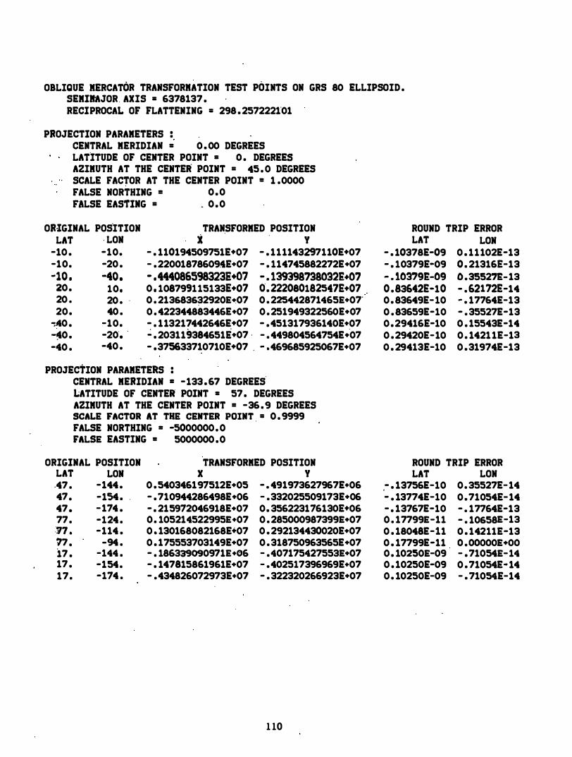
OBLIQUE MERCATOR TRANSFORMATION TEST POINTS ON GRS 80 ELLIPSOID . SEMIRAJOR . AXIS = 6378137 . RECIPROCAL OF FLATTENING = 298 . 2572221·01

PROJECTION PARAMETERS : CENTRAL MERIDIAN = 0 . 00 DEGREES LATITUDE OF CENTER POINT = O . DEGREES A2IMUTH AT THE CENTER POINT = 45 . 0 DEGREES SCALE FACTOR AT THE CENTER POINT = 1 .0000 FALSE NORTHING = 0 . 0 FALSE EASTING = _ 0 . 0

ORIGINAL POS·ITION LAT . LON

-10 . -10. -10. -20 . -10 . -40.

20 . 10. 20 . 20 • . 20 . 40 .

-;40 . -10. -!l0 . -20· • .

-40 . -40 .

TRAN.SFORMED POSITION I .

Y - . 110194509751E+07 - . 1 1 1143297110E+07 - . 220018786094E+07 - . 114745882272E+07 - .444086S98323E+07 - . 1393987g80g2E.07 0 . 1087991 15133E+07 0. 222080182547E+07 0 . 213683632920E�07 0 . 225442871465E.07· 0 . 422344883446E.07 0 . 251949322560E.07 - . 1 13217442646E+07 - . 451317936140E.07 � . 203119384651E.07 · - . 449804564754E.·07 - • 375633710710E+07 . - • 469685925067E+07

PROJECTION PARAMETERS : CENTRAL MERIDIAN = - 133 . 67 DEGREES LATITUDE OF CENTER POINT = 57 . DEGREES AZIMUTH AT THE CENTER POINT = -36 . 9 DEGREES SCALE FACTOR AT THE CENTER POINT . = 0 . 9999 FALSE NORTHING = -5000000 . 0 FALSE EASTING = 5000000 . 0

ORIGINAL POSITION LAT LON .47 . -144 . 47 . -154 • .

47 . - 114 . 77 . -124 . :'!/7 . - 1 14 . '17 . -94 . 17 . -144 . 17 . -154 . 1 7 . -114 .

TRANSFORMED POSITION X Y

0 . 540346191512E+05 - . 491973627967E+06 - . 710944286498E.06 - . 332025509173E+06 - . 215912046918E+07 0 . 356223116130E+06 0 . 105214522995E+07 0 . 285000987399E+07 0 . 130168082168E+07 0 . 292134430020E+07 0 . 175553703149E+07 0 . 318750963565E+07 - . 186339090971E+06 - . 407175427553E+07 - . 147815861961E+07 - . 402517396969E+07 - . 434826072973E+07 - . 322320266923E+07

1 10

ROUND TRIP ERROR LAT LON

- . 10378E-09 0 . 1 1 102E-13 - . 10379E-09 0 . 21316£-13 - . 10�9E-09 0 . 35527£- 13 0 . 83642E-10 - . 62172E-14 0 . 83649E- l0 - . 17764E-13 0 . 83659E-l0 - . 35527E-13 0 . 29416E-l0 0 . 15543E-14 0 . 29420E- 10 0 . 1421 1E-13 0 . 29413E-l0 0 . 31974E-13

ROUND TRIP ERROR LAT

.- . 13756E-l0 - . 13774E-l0 - . 13767E-l0 0 . 17799E-11 0 . 18048E-l1 0 . 17799E-11 0 . 10250E-09 0 . 10250E-09 0 . 10250E-09

LON 0 . 35527E- 14 0 . 71054E- 14 - . 17764E-13 - . 10658E-13 0 . 14211£-13 O . OOOOOE+OO - . 71054E- 14 0 . 71054E- 14 - . 71054E-14

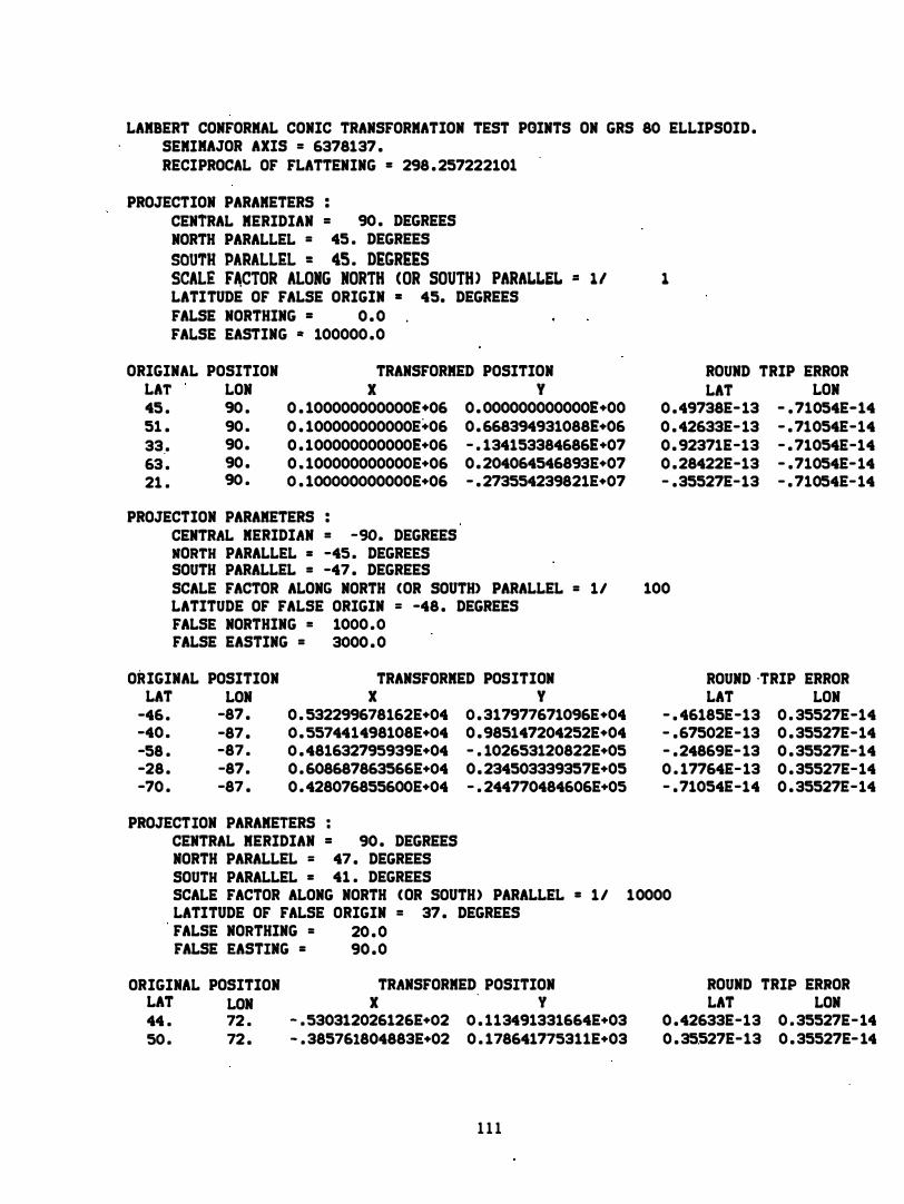
LAMBERT CONFORMAL CONIC TRANSFORMATION TEST POINTS ON GRS 80 ELLIPSOID . SEMI MAJOR AXIS = 6378137 . RECIPROCAL OF FLATTENING = 298 . 257222101

PROJECTION PARAMETERS : CENTRAL MERIDIAN = 90 . DEGREES NORTH PARALLEL = 45 . DEGREES SOUTH PARALL&L = 45. D;GR;;S SCALE F�CTOR ALONG NORTH (OR SOUTH) PARALLEL = 1 / 1 LATITUDE OF FALSE ORIGIN = 45. DEGREES FALSE NORTHING = 0 . 0 . FALS£ £ASTING = 100000 . 0

ORIGINAL POSITION TRANSFORMED POSITION LAT LON 45 . 90 . 51 . 90 . 33 . 90 . 63 . 90 . 21 . 90 .

X 0 . 100000000000£+06 0 . 100000000000E+06 0 . 100000000000£+06 0 . 100000000000E+06 0 . 100000000000£+06

PROJECTION PARAMETERS : CENTRAL MERIDIAN = -90. DEGREES NORTH PARALLEL = -45 . DEGREES SOUTH PARALLEL = -47 . DEGREES

Y 0 . 000000000000£+00 0 . 668394931088£+06 - . 134153384686£+07 0 . 204064546893E+07 - . 273554239821E+07

ROUND TRIP ERROR LAT LON

0 . 49738E- 13 - . 71054E-14 0 . 42633E- 13 - . 71054E-14 0 . 92371E-13 - . 71054E-14 0 . 28422E-13 - . 71054E- 14 - . 35527E-13 - . 71054E- 14

SCALE FACTOR ALONG NORTH (OR SOUTH) PARALLEL = 1/ 100 LATITUDE OF FALSE ORIGIN = -48 . DEGREES FALSE NORTHING = 1000 . 0 FALSE EASTING = 3000 . 0

ORIGINAL POSITION LAT LON

-46 . -87 . -40 . -87 . -58 . -87 . -28 . -87 . -70 . -87 .

TRANSFORMED POSITION X Y

0 . 532299678162E+04 0 . 317977671096E+04 0 . 557441498108E+04 0 . 985147204252E+04 0 . 481632795939E+04 - . 102653120822E+05 0 . 608687863566E+04 0 . 234503339357E+05 0 . 428076855600E+04 - . 244770484606E+05

PROJECTION PARAMETERS : CENTRAL MERIDIAN = 90 . DEGREES NORTH PARALLEL = 47 . DEGREES SOUTH PARALLEL = 41 . DEGREES

ROUND ·TRIP ERROR LAT LON

- . 46185E-13 0 . 35527E-14 - . 67502E-13 0 . 35527E-14 - . 24869E- 13 0 . 35527E-14 0 . 17764E- 13 0 . 35527E-14 - . 71054E-14 0 . 35527E-14

SCALE FACTOR ALONG NORTH (OR SOUTH) PARALLEL = 1 / 10000 LATITUDE OF FALSE ORIGIN = 37 . DEGREES FALSE NORTHING = 20 . 0 FALSE EASTING = 90 . 0

ORIGINAL POSITION LAT LON 44 . 72 . 50 . 72 .

TRANSFORMED POSITION X

. Y - . 530312026126E+02 0 . 113491331664E+03 - . 385761804883E+02 0 . 178641775311E+03

1 1 1

ROUND TRIP ERROR LAT LON

0 . 42633E-13 0 . 35527E- 14 0 . 35527E-13 0 . 35527E- 14

32 . 62. 20 .

72 . 72 . 72 • .

- . 820463175976E+02 - . 172831214965E+02 - . 890450684381E+01 0 . 312375413700E+03 - . 112203315241E+03 - . 153204170845E+03

PROJECTION PARAMETERS : . CENTRAL RERIDIAN = �90 . DEGREES I NORTH PARALLEL = -41 . DEGREES SOUTH PARALLEL = -63 . DEGREES

0 . 74607E-13 0 . 35527E-14 0 . 39080E-13 0. 35527E-14 - . 21316E-13 0 . 35527E-14

SCALE FACTOR ALONG NORTH ( OR SOUTH) PARALLEL = 1/1000000 LATITUDE OF FALSE ORIGIN = -72 . DEGREES FALSE NORTHING = 0 . 3 FALSE EASTING = 2 . 7

ORIGIMAL POSITIOM LAT LON

-52 . -9 . -46. ·9. -64 . -9 . -34. -9 . -76 . -9 .

TRANSFORKED POSITION X Y

0 . 708627916328E+01 - . 216266453769E+00 0 . 767742915085E+01 0 . 690324367425E-01 0 . 589648620445E+01 - . 790480474290E+00 0 . 888326834518E+01 0 .650990639417E+00 0 . 463806124612E+01 - . 139781744790E+01

1 12

ROUND TRIP ERROR LAT LON

- . 46185E-13 - . 66613E-15 - . 56843E-13 - . 66613E-15 - . 35527E-13 - . 66613E-15 - . 81712E-13 - .66613E-15 - . 21316E-13 - . 66613E-15

POLYCONIC TRANSFORMATION TEST POINTS ON GRS 80 ELLIPSOID SEftlftAJOR AXIS = 6378137 .

. RECIPROCAL OF FLATTENING = 298 . 257222101

PROJECTION . PARAMETERS : CENTRAL MERIDIAN = O . DEGREES . LATITUDE OF GRID ORIGIN = O . DEGREES SCALE .FACTOR ALONG CENTRAL MERIDIAN = 1/ 1 FALSE EASTING = 0 . 0

ORIGINAL POSITION TRANSFORMED POSITION LAT LON X Y

O • . O . O . OOOOOOOOOOOOE+OO O . OOOOOOOOOOOOE+OO O . -2 . - . 222638981587E+06 O . OOOOOOOOOOOOE+OO O . 4 . O . 445277963173E+06 O . OOOOOOOOOOOOE+OO O . -6. - . 667916944760E+06 O . OOOOOOOOOOOOE+OO o . 8 . 0 . 890555926346E+06 O . OOOOOOOOOOOOE+OO

PROJECTION PARAMETERS : CENTRAL MERIDIAN = 90 . DEGREES LATITUDE OF GRID ORIGIN = -25 . DEGREES SCALE FACTOR ALONG CENTRAL . MERIDIAN = 1/ 100 FALSE EASTING = 10000 . 0

ORIGINAL POSITION LAT LON

-22 . 90 . -22 . 88 . -22 . 94 . -22 . 84 . -22 . 98 .

TRANSFORMED POSITION X , Y

0 . 100000000000E+05 0 . 332253691352E+04 0 . 793481586721E+04 0 . 330903430263E+04 0 . 141300151490E+05 . 0 . 326852877871E+04 0 . 380586000770E+04 0 . 320102726762E+04 0 . 182572057273E+05 0 . 310654131114E+04

PROJECTION PARAMETERS : CENTRAL .MERIDIAN = -180 . DEGREES LATITUDE OF GRID ORIGIN = 50 . DEGREES SCALE FACTOR ALONG CENTRAL MERIDIAN = 1/ 10000 FALSE EASTING = 200 . 0

ORIGINAL POSITION TRANSFORMED POSITION LAT LON 68 . -180 . 68 . · -182 . 68 . -176 . 68 . - 186 . 68 . -17� .

X 0 . 200000000000E+03 0 . 191637154283E+03 0 . 216716932271E+03 0 . 174946490328E+03 0 . 233363846271E+03

PROJECTION PARAMETERS :

y 0 . 200503560859E+03 0 . 200638903680E+03 0 . 201044790387E+03 0 . 201720795857E+03 0 . 202666212049E+03

CENTRAL MERIDIAN = · 270 . DEGREES LATITUDE OF GRID ORIGIN = -75 . DEGREES SCALE FACTOR ALONG C£NTRAL M£RIDIAN • 1 /1000000 FALSE EASTING · = . 3 . 0 . .

1 1 3

ROUND TRIP ERROR LAT LON

O . OOOOOE+OO O . OOOOOE+OO O . OOOOOE+OO O . OOOOOE+OO O . OOOOOE+OO O . 22204E- 15 O . OOOOOE+OO O . OOOOOE+OO O . OOOOOE+OO - . 44409E-15

ROUND TRIP ERROR LAT LON

- . 15016£-08 - . 11054£- 14 - . 41594E-09 - . 17808E-06 0 . 28557£-08 0 . 35678E-06 0 . 83267E-08 - . 53674E-06 0 . 16025£-07 0 . 71859E-06

ROUND TRIP £RROR LAT LON

0 .44052E-08 0 . 00000£+00 0 . 36550E-10 - . 71821E-06 - . 13159£-07 0 . 14383£-05 - . 34925£-07 - . 21622E-05 - .65744£-07 0 . 28917£-05

ORIGINAL POSITION TRANSFORME"D POSITION ROUND TRIP ERROR LAT LON X Y LAT LON

6 � 270 . 0 . 300000000000E+01 0 . 8990407�4253£+01 0 . 15740E-08 0 . 00000£+00 6". 268 . 0 . 277857305116£+01 0 . 899081150674£+01 - . 42497£-09 - . 10967£-05 6 . 274 . 0 . 344285094977E+01 0 . 899202339399£+01 - . 64194E-08 0 . 21975E-05 6 . 264 . 0 . 233573094508£+01 0 . 899404318816£+01 - . 16397£-07 - . 33062£-05 , . 278 . 0 . 388567831651E+01 0 . 899687086234E+01 - . 30334E-07 0 . 44269E-05

1 14

AZIMUTHAL EQUIDISTANT TRANSFORMATION TEST POINTS ON GRS " 80 ELLIPSOID . SEMIMAJOR AXIS = 6378137 . RECIPROCAL OF FLATTENING = 298 . 257222101

PROJECTION PARAMETERS : CENTRAL MERIDIAN = O . DEGREES LATITUDE OF CENTER POINT • " O . DEGREES seALE rAe,oR A' eEN'ER POIN' = 11 1 FALSE NORTHING = 100000 . 0 FALSE EASTING = 0.0

ORIGINAL POSITION TRANSFORMED POSITION LAT LON X Y

O . O . O .OOOOOOOOOOOOE+OO 0 . 10000oo000ooE+06 O . -4 . - . 445277963173E+06 0 . 10oooo000000E+06 O . 8 . 0 . 890555926346E+06 0 . lOO000000000E+06 O . - 12 . - . 133583388952E+07 0 . 100000000000E+06 o . 16. 0 . 178111185269E+07 0 . 100000000000E+06

PROJECTION PARAMETERS : CENTRAL MERIDIAN = 90 . DEGREES LATITUDE OF CENTER POINT = -25 . DEGREES SCALE FACTOR AT CENTER POINT = 11 " 100 FALSE NORTHING = " 3000 . 0 FALSE EASTING = 10000 . 0

ORIGINAL POSITION TRANSFORMED POSITION LAT LON

-21 . 90 . -21 . 86 . -21 . 98. -21 . 78 . -21 . 106 .

X 0 . 100000000000E+05 0 . 583832194842E+04 0 . 183202425567E+05 - . 247254370047E+04 0 . 266153580596E+05

PROJECTION PARAMETERS :

. y 0 . 742977300029E+04 0 . 737140323260E+04 0 . 7196101.7008E+04 0 . 690328843789E+04 0 . 649199356040E+04

CENTRAL MERIDIAN = - 180 . DEGREES LATITUDE OF CENTER POINT = 50 . DEGREES SCALE FACTOR AT CENTER POINT = 11 10000 FALSE NORTHING = 90 . 0 FALSE EASTING = 200 . 0

ORIGINAL POSITION " TRANSFORMED POSITION LAT LON 58 . - 180 . 58 . - 184: . 58 . - 172 . 58 . - 192 . 58 . - 164 .

X 0 . 200000000000E+03 0 . 176282478599E+03 0 . 247358939396E+03 0 . 129151985260E+03 0 . 294108239265E+03

y 0 . 179043563031E+03 0 . 179702783757E+03 0 . 181679446287E+03 0 . 184970535438E+03 0 . 189570971987E+03

1 1 5

ROUND TRIP ERROR "LAT LON

O . OOooOE+OO O . OOOooE+oo - . 24638E- 15 0 . 62172E-14 - .49156E- 15 - . 13101E-13 - . 73434E-15 0 . 20872E- 13 - . 97355E- 15 - . 31974E-13

ROUND TRIP ERROR LAT LON

- . 17150E-07 - . 71054E-14 - . 26883E-07 0 . 21661E-07 - . 24700E-07 - . 38441E-07 0 . 93255E-07 - . 21072E-06 0 .53314E-06 0 . 15008E-05

ROUND TRIP ERROR LAT LON

0 . 38432E-07 O . OOooOE+OO 0 . 64368E-07 - . 44858E-07 0 . 16013E-06 0 . 22781E-06 0 . 37251E-06 - . 83417E-06 0 . 75603E-06 0 . 24376E-05

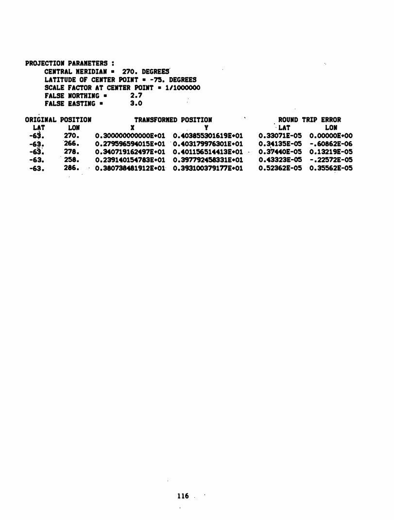
PROJECTION PARAMETERS : CENTRAL MERIDIAN . 270 . DEGREES" LATITUDE OF CENTER POINT • -75. DEGREES SCALE FACTOR AT CENTIR POINT • 111000000 FALSE NORTHING . 2 . 7 FALSE lASTING • 3 . 0

ORIGINAL POSITION LAT LON

-6� . 270 . -63 . 266 . -63� 278 . -63. 258. -63 . 286 .

TRANSFORMED POSITION X " Y

0 . 300000000000E.Ol 0 . 4038553016191.01 0 . 279596594015E.01 " 0 . 403179976301E+01 0 . 3407191624971+01 0 . 4011565144131.01 0 . 239140154783E+01 0 . 397792458331E.Ol 0 . 3807384819121.01" 0 . 3931003791771.01

1 16

ROUND TRIP ERROR " LAT

0 . 330711-05 0 . 3,4135E-05 0 . 374401-05 0 .43323E-05 0 .523621-05

LON 0 . 000001+00 - . 60862E-06 0 . 132191-05 - . 22572E-05 0 . 355621-05

..... ..... .....,

DATUM TRANSFORMATION TEST POINTS FROM NAD 27 ( SEMIMAJOR AXIS • 6378206 . 4 , , RECIPROCAL OF FLATTENI NG = 294 . 978698) TO NAD 83 ( SEMIMAJOR AXIS = 6378137 . , RECIPROCAL OF FLATTENI NG = 298 . 257222101 ) .

PROJECTION PARAMETERS : DELTA X = o . METERS DELTA Y = O . METERS DELTA Z = O . METERS OMEGA = 0 . 0 SECONDS EPSILON = 0 . 00 SECONDS PSI • 0 . 0 SECONDS DELTA K = O . OOE+OO

POSITION ON NAD 83 LAT LON HT

0 . 000000000 0 . 000000000 1069 . 40000

POSITION ON NAD 27 LAT LON ELEV NSEP 0 . 0 o. 1000 . o .

22 . 4 45 . -2000 . -20 . 44 . 8 -90 . 3000 . 40 .

-67 . 2 -135 . -4000 . -60 .

22 . 398489256 45 . 000000000 - 1985 . 04682 44 . 797860212 -90 . 000000000 2991 . 47876

-67 . 198471215 - 135 . 000000000 -4192 . 68196 -89 . 6 180 . 5000 . 80 .

PROJECTION PARAMETERS :

-89 . 599970182 180 . 000000000 4911 . 49748

DELTA X = 20 . METERS DELTA Y = -25 . METERS DELTA 2 = , 5 . METERS OMEGA = 0 . 3 SECONDS EPSILON = 0 . 05 SECONDS PSI = 0 . 1 SECONDS DELTA K = - . 10E-06

POSITION ON NAD 27 LAT LON ELEV NSEP 0 . 0 O . 1000 . O .

22. 4 45. -2000. -20. 44 . 8 -90 . 3000 . 40 .

-67 . 2 -135. -4000. -60. -89 . 6 180 . 5000 . 80 .

POSITION ON NAD 83 LAT LON HT

0 . 000073176 -0. 000307874 1088 . 76218 22 . 398553066 44 . 999619615 - 1 987 . 04499 44 . 797747595 -89 . 999858081 301 2 . 10988

-67 . 198434372" -134 . 999277757 - 4196 . 55394 -89 . 600176311 -179 . 966055878 4905 . 72204

ROUND TRIP ERROR LAT

O . OOOOOE+OO -0 . 23093E- 12 -0 . 14815E-11

0 . 10232E- 11 0 . 00000£+00

LON O . OOOOOE+OO O . OOOOOE+OO 0 . 71054E-14 0 . 35527E-14 O . OOOOOE+OO

NSEP O . OOOOOE+OO

- 0 . 10245E-07 - 0 . 16391E-06 -0 . 26962E-06

O . OOOOOE+OO

ROUND TRI P ERROR LAT

0 . 15830E-09 0 . 35650E-09

-0 . 1 1269E-l0 0 . 43280E-09 0 . 38503£-09

LON NSEP -0 . 221 1 9E-09 -0. 55780E-04

0. 1 1674E-09 -0. 46066E-04 -0 . 50204E-09 0 . 16177E-04 -0 . 21319E-09 0 . 35572E-05

0. 38271E-07 - 0 . 16804E-04

PROJECTION PARAMETERS : DELTA I . -40. METERS DELTA y . SO. METERS DELTA Z . -SO. IETERS OKEGA • -0. 9 SECONDS EPSILON • - . 15 SECONDS PSI • - . 2 SECONDS DELTA K • 0 . 20E-05

POSITIOI 01 lAD 83 LAT " LON

POSITION 01 lAD 27 LAT LON ELEV" NSEP 0 .0 0. " 1000. o.

22 . 4 45 . -2000. -20 . 44 . 8 -90 . 3000 . 40.

-67.2 -135. -4000. -60.

-0.000508041 0 . 000699086

-89.6 180. 5000. 80.

= PROJECTIOI PARAMETERS :

22. 398037183 45 . 000840080 44.797815914 -90 . 000200507

-67. 198693505 -135. 001384358 -89.599559985 179. 930326288

� DELTA I" • 60. METERS DELTA y . -75 . METERS DELTA Z · -375 . K£TERS OKEGA • 2 . 1 SECOIDS £PSILON • 0 . 35 SECOIOS PSI = - . 3 SECONDS DELTA K • - .30£-04

POSITIOI 01 lAD 27 POSITIOI 01 lAD 83 LAT LOI " £LEV ISEP LAT LON 0 .0 o. 1000 . O . -0.003474778 -0. 001256965

22 . 4 45. -2000. -20. 22.395269447 44 . 998493320 44 .8 -90. 3000. 40 . 44.795094311 -89 . 999743168

-67.2 �135 . -4000. -60 . -67 . 199564450 -134 . 998352192 -89.6 180. 5000. 80 . -89.600446926 -179 . 890522738

RT 1042 . 15914

- 1984 . 81722 2933 .49403

-4136 . 62038 4974 . 49897

HT 938 . 03700

-2328. 95865 2589. 39877

-4033 .58247 5095 . 21984

ROUHD TRIP £RROR LAT LON ISEP

-0. 41706£-10 - 0 . 30244E�09 -0. 47410E-03 0 . 13008£-08 0 . 21483E-08 -0 . 34293E-03 0 . 11601E-09 -0. 42401£-08 -0.85144£-04 0 . 20128E-08 ·-0. 4932OE-08 0 . 12569£-03 0 .32724E-08 0.83439£-07 0 . 18302£-04

ROU.D TRIP ERROR LAT LON lSEP

0 . 10309£-06 0 . 88658£-08 -0 . 37838£-02 0 . 10160E-06 0 . 27692E-07 0 .23364£-02 0 . 81340E-07 - 0 . 38158£-07 0 .69795E-02 0 .49519£-07 -0. 70343E-07 -0.99545£-02 0. 29460£-07 - 0 . 14059£-05 -0 . 11299£-01

REFERENCES Adams , Oscar S . , 1949 : lati tude devel opments i n connection wi th geodesy and

cartography , s�ecial Publ ication 67 , U . S . Coast and Geodeti c Su rvey , Washi ngton , D • • , pp . 89 , 125, National Geodeti c Informati on Center, NOAA, Rockvi l le , MD 20852.

AYres , James A. , 1983 : Ci rcular Letter 44/1983 , International Hydrographic Organization , Monaco .

Berry , Ral ph M. , 1971 : The Michigan coordinate system, paper presented to Mi chigan Association of Regi stered Land Surveyors , pp. 22-25, Nati onal Geodeti c I nformation Center , NOAA, Rockvi l le , MD 20852 �

Bowring , B . R. , 1976 : Transformation from spacial to geographi ca l coordi nates , Survey Revi ew. no . 181 , pp . 323-327.

Cl ai re , Charles N. , 1968 , rev . 1973 : State pl ane coordi nates by automatic data process i ng , Publ ication 62-4 , U. S . Coast and Geodeti c Survey , Washington , D . C . , National Geodetic Informati on Center, NOAA , Rockvi l l e , MD 20852 .

Deetz , Charles H . , and Adams , Oscar S . , 1944: Elements of map projection wi th appl i cations to map and chart construction , Special Publ i cation 68 , 5th ed . , U . S . Coast and Geodeti c Survey; Washi ngton , D.C. , pp . 1 12-114.

Hoti ne , Martin , 1945-46 : The orthomorphi c projecti on of the spheroid , Empi re Survey Review , vol s . V I I I and I X , no . 62-66 .

Mi tchel l , Hugh C . , and Simmons , Lanci ng G . , 1945 : The state coordinate systems (a manual for surveyors ) , Special Publ i cation 235 , U.S. Coast and Geodeti c Survey , Washington , D. C.

Pfeifer, Ludvi k , 1980 : Input Formats and Speci fications of the National Geodeti c Survey Data Base , vol . I : Horizontal control data , Federal Geodetic Control Committee , pp . B-1 - B-2 , National Geodeti c Information Center. NOAA, Rockvi l le , MD 20852. .

Rapp , Richard H . , 1981 : Transformation of geodeti c data between reference datums , Geometri c Geodesy , vol . I I , Ohio State Univers ity , Col umbus , pp . 53-57 , 66.

Snyder , James P. , 1983: Map projections used by the U .S . Geol og ical Survey , Geol ogical Survey Bul l eti n 1532 , 2nd ed . , U . S . Geol ogical Survey , washington , b. t. , 313 pp.

Thomas , Paul D. , 1952 : Conformal projections in geodesy and cartography , Special Publ i cation 251 , U . S . Coast and Geodeti c Survey , Washi ngton , D .C . pp . 85-90.

1 1 9

Vincenty , T. , (National Geodetic Survey . National Oceanic and Atmospheric Administration . u.s. Department of ·Commerce , Rockvi l le , MD) 1984a : Transverse Mercator projection formulas for GRS80 el l i psoi d , 7 pp • • Aug. 31 , 1984 (unpubl ished fi le report) . . .

Vincenty , T. , (National Geodetic Survey , National Oceanic and Atmospheric Admini stration , ' U .S . Department of Commerce , Rockvi l le , MO) 1984b : ·Obl ique Mercator projection formulas for GRS80 el l i psoi d . 4 pp. , Sept. 1 , 1984 (unpubl i shed fi l e report ) . .

Vincenty, T. , (National Geodetic Survey, National Oceani c and · Atmospheric ·�mini stration , U .S . Department of Commerce . Rockvl l le � MO) 1985 : Lambert conformal conic projection formulas for GRS80 el l ipsoi d , 5 pp. , Mar. 1 . 1985 (unpubl i shed fi l e report) . . .