Convolutional Neural Networks

CSC 4510/9010Andrew Keenan

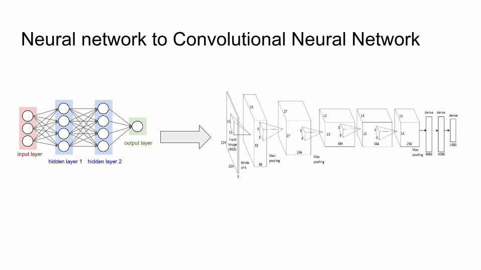
Neural network to Convolutional Neural Network

0.4

0.7

0.3

Neural Network Basics

0.4

0.7

0.3

NetworkIndividual Neuron

Backpropagation1. Compute forward pass of network2. Calculate error from expected value3. Backpropagate error signal to adjust

weights4. Repeat until convergence

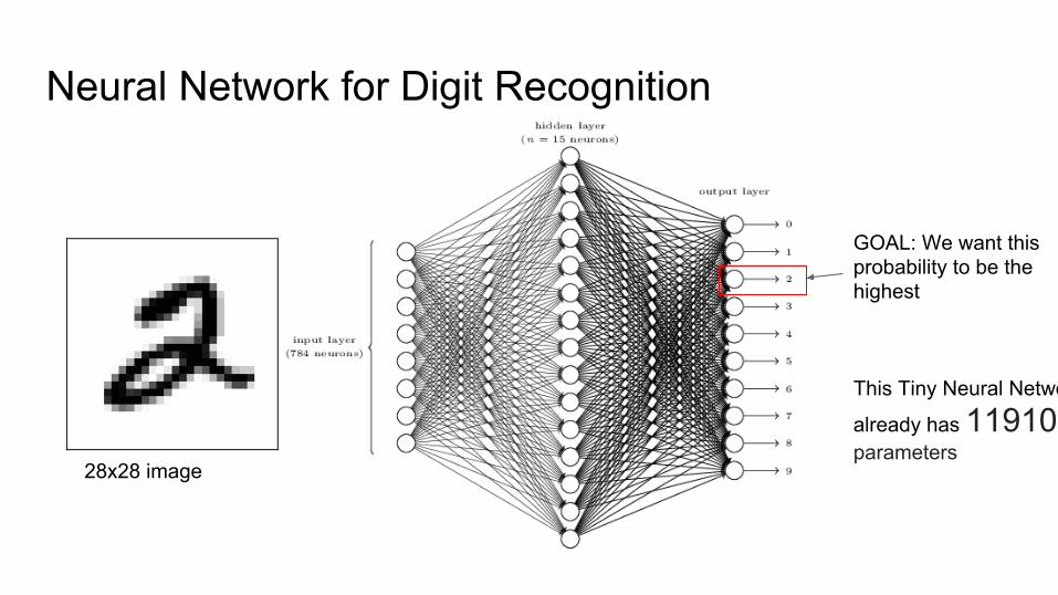
Neural Network for Digit Recognition

28x28 image

GOAL: We want this probability to be the highest

This Tiny Neural Network

already has 11910 parameters

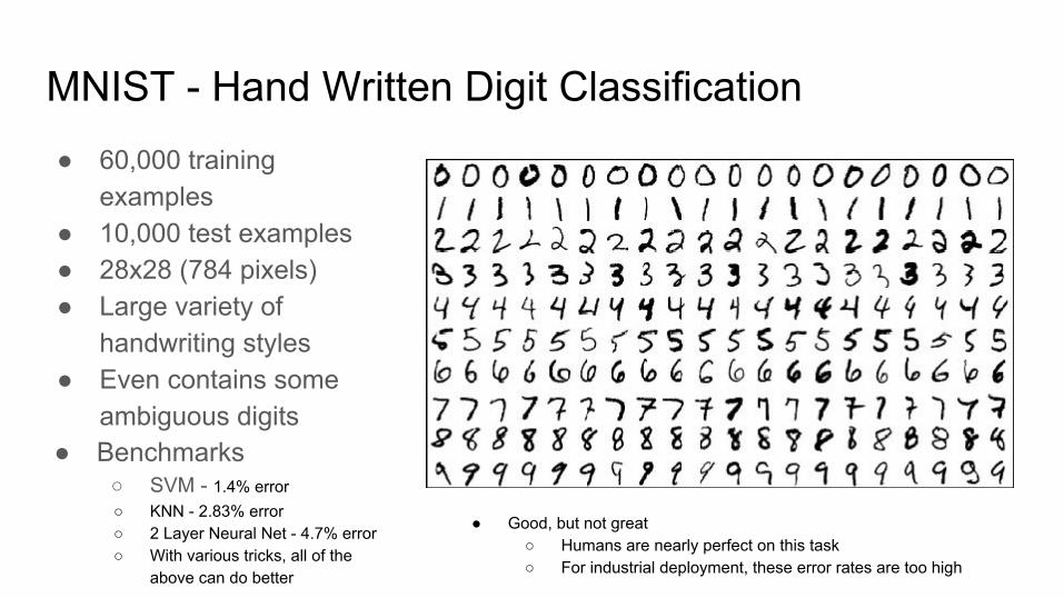
MNIST - Hand Written Digit Classification● 60,000 training

examples● 10,000 test examples● 28x28 (784 pixels)● Large variety of

handwriting styles● Even contains some

ambiguous digits● Benchmarks

○ SVM - 1.4% error○ KNN - 2.83% error○ 2 Layer Neural Net - 4.7% error○ With various tricks, all of the

above can do better

● Good, but not great○ Humans are nearly perfect on this task○ For industrial deployment, these error rates are too high

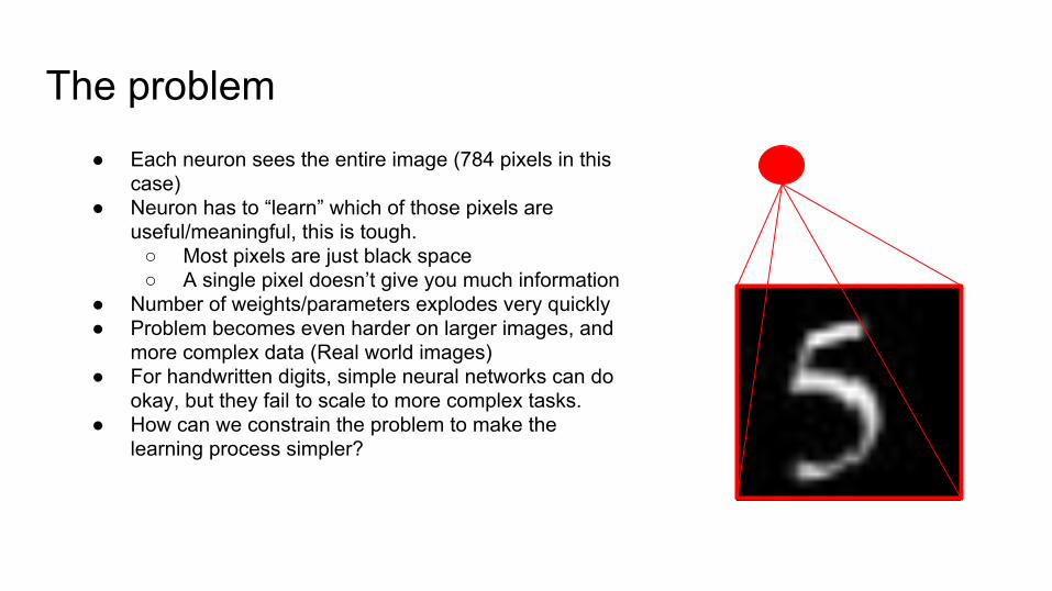
The problem● Each neuron sees the entire image (784 pixels in this

case)● Neuron has to “learn” which of those pixels are

useful/meaningful, this is tough.○ Most pixels are just black space○ A single pixel doesn’t give you much information

● Number of weights/parameters explodes very quickly● Problem becomes even harder on larger images, and

more complex data (Real world images)● For handwritten digits, simple neural networks can do

okay, but they fail to scale to more complex tasks.● How can we constrain the problem to make the

learning process simpler?

Permutation InvarianceThe simple Neural Network can be trained on permuted version of data

As long as permutation is consistent across entire dataset.

Neural Network has no problem with this, but the problem becomes impossible for Humans. What does this say about the difference between how we process images, and how Neural Nets do?

=

f( x1*w1 + x2*w2 + x3*w3…..) = f( x3*w3 + x2*w2 + x1*w1…….)

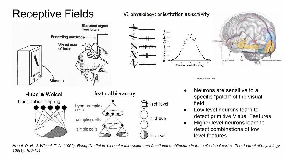
Receptive Fields

Hubel, D. H., & Wiesel, T. N. (1962). Receptive fields, binocular interaction and functional architecture in the cat's visual cortex. The Journal of physiology, 160(1), 106-154.

● Neurons are sensitive to a specific “patch” of the visual field

● Low level neurons learn to detect primitive Visual Features

● Higher level neurons learn to detect combinations of low level features

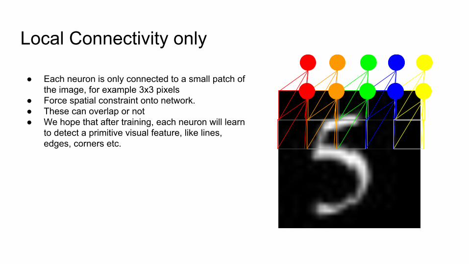
Local Connectivity only

● Each neuron is only connected to a small patch of the image, for example 3x3 pixels

● Force spatial constraint onto network. ● These can overlap or not● We hope that after training, each neuron will learn

to detect a primitive visual feature, like lines, edges, corners etc.

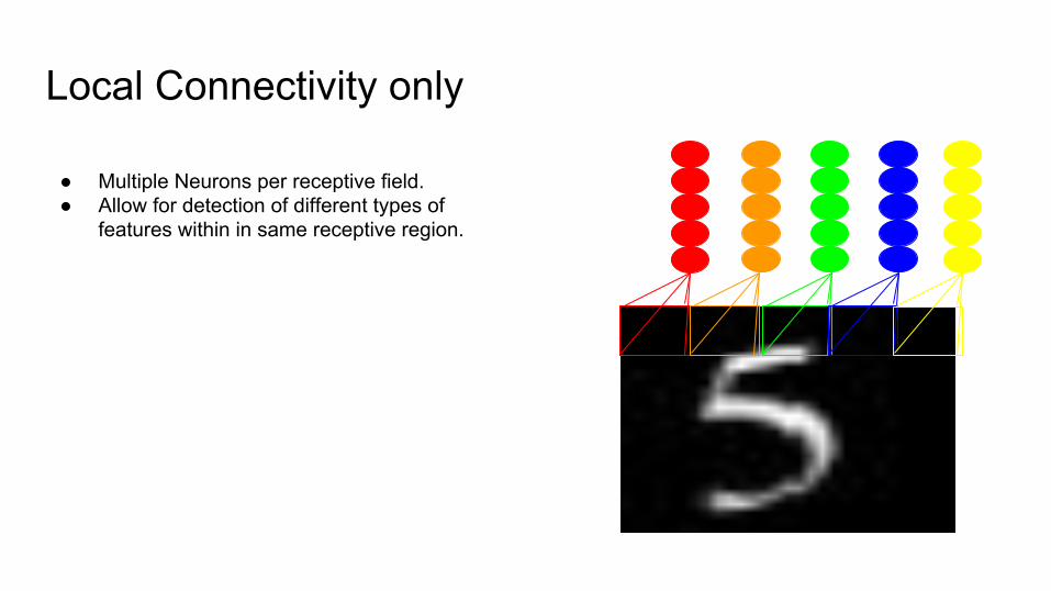
Local Connectivity only

● Multiple Neurons per receptive field.● Allow for detection of different types of

features within in same receptive region.

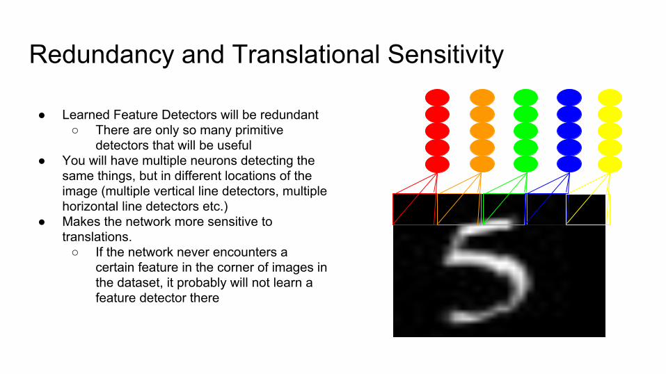
Redundancy and Translational Sensitivity

● Learned Feature Detectors will be redundant○ There are only so many primitive

detectors that will be useful● You will have multiple neurons detecting the

same things, but in different locations of the image (multiple vertical line detectors, multiple horizontal line detectors etc.)

● Makes the network more sensitive to translations.

○ If the network never encounters a certain feature in the corner of images in the dataset, it probably will not learn a feature detector there

Share Parameters between columns

● Learn one column of neurons, and “sweep” it across the entire image.

● As an added bonus, we reduce the number of parameters dramatically

○ 784 parameters per neuron, vs. 9 for a 3x3 patch.

○ This helps us train our network much faster, less parameters = smaller weight space to search through

Share Parameters between neurons

● Learn one column of neurons, and “sweep” it across the entire image.

● As an added bonus, we reduce the number of parameters dramatically

○ 784 parameters per neuron, vs. 9 for a 3x3 patch.

○ This helps us train our network much faster, less parameters = smaller weight space to search through

Share Parameters between neurons

● Learn one column of neurons, and “sweep” it across the entire image.

● As an added bonus, we reduce the number of parameters dramatically

○ 784 parameters per neuron, vs. 9 for a 3x3 patch.

○ This helps us train our network much faster, less parameters = smaller weight space to search through

Share Parameters between neurons

● Learn one column of neurons, and “sweep” it across the entire image.

● As an added bonus, we reduce the number of parameters dramatically

○ 784 parameters per neuron, vs. 9 for a 3x3 patch.

○ This helps us train our network much faster, less parameters = smaller weight space to search through

Share Parameters between neurons

● Learn one column of neurons, and “sweep” it across the entire image.

● As an added bonus, we reduce the number of parameters dramatically

○ 784 parameters per neuron, vs. 9 for a 3x3 patch.

○ This helps us train our network much faster, less parameters = smaller weight space to search through

Share Parameters between neurons

● Learn one column of neurons, and “sweep” it across the entire image.

● As an added bonus, we reduce the number of parameters dramatically

○ 784 parameters per neuron, vs. 9 for a 3x3 patch.

○ This helps us train our network much faster, less parameters = smaller weight space to search through

Share Parameters between neurons

● Learn one column of neurons, and “sweep” it across the entire image.

● As an added bonus, we reduce the number of parameters dramatically

○ 784 parameters per neuron, vs. 9 for a 3x3 patch.

○ This helps us train our network much faster, less parameters = smaller weight space to search through

Share Parameters between neurons

● Learn one column of neurons, and “sweep” it across the entire image.

● As an added bonus, we reduce the number of parameters dramatically

○ 784 parameters per neuron, vs. 9 for a 3x3 patch.

○ This helps us train our network much faster, less parameters = smaller weight space to search through

Share Parameters between neurons

● Learn one column of neurons, and “sweep” it across the entire image.

● As an added bonus, we reduce the number of parameters dramatically

○ 784 parameters per neuron, vs. 9 for a 3x3 patch.

○ This helps us train our network much faster, less parameters = smaller weight space to search through

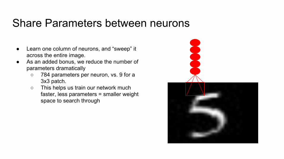
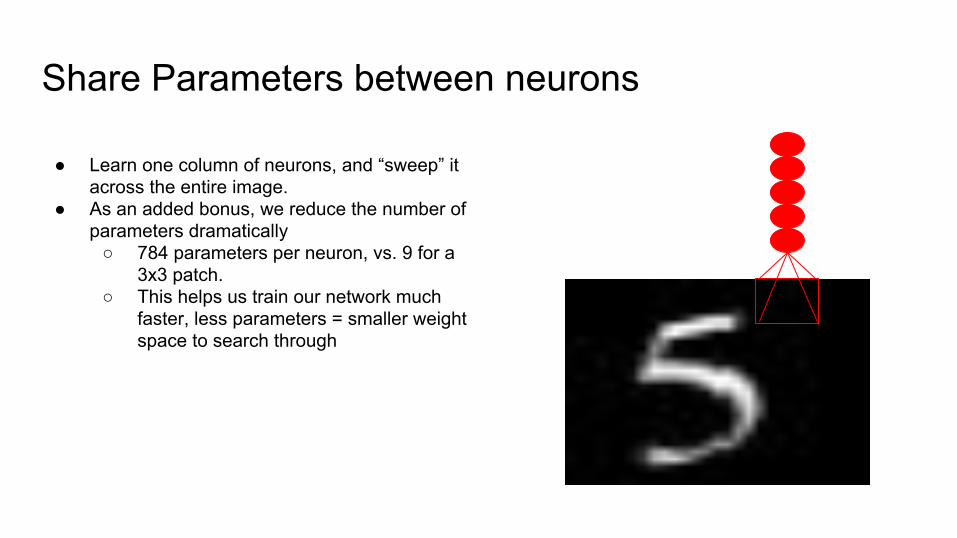
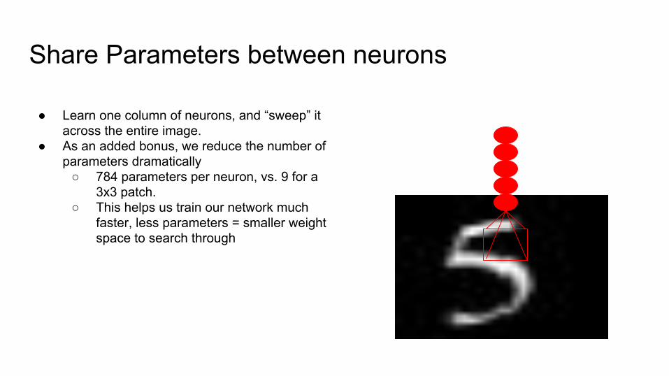
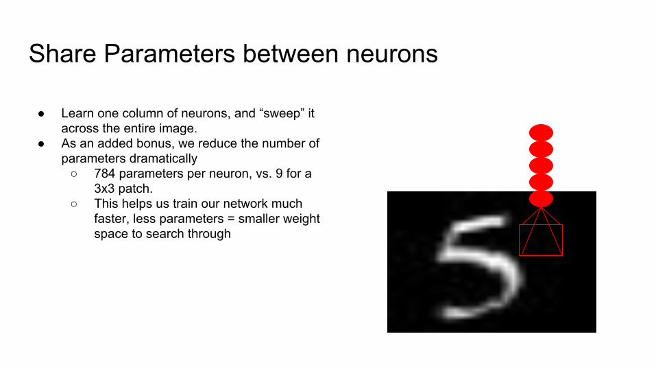
Share Parameters between neurons

● Learn one column of neurons, and “sweep” it across the entire image.

● As an added bonus, we reduce the number of parameters dramatically

○ 784 parameters per neuron, vs. 9 for a 3x3 patch.

○ This helps us train our network much faster, less parameters = smaller weight space to search through

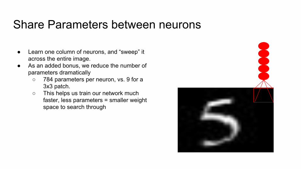
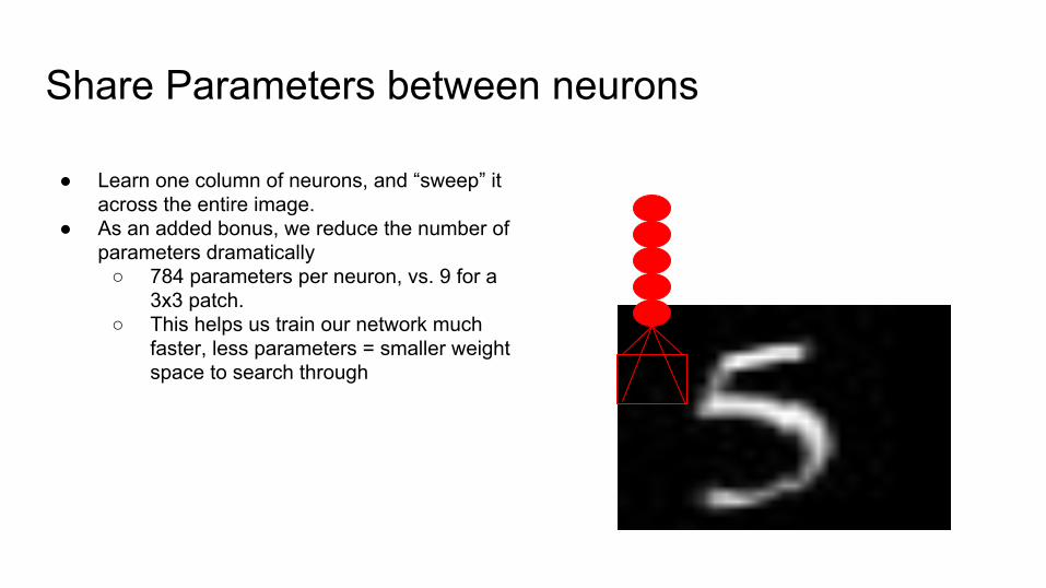
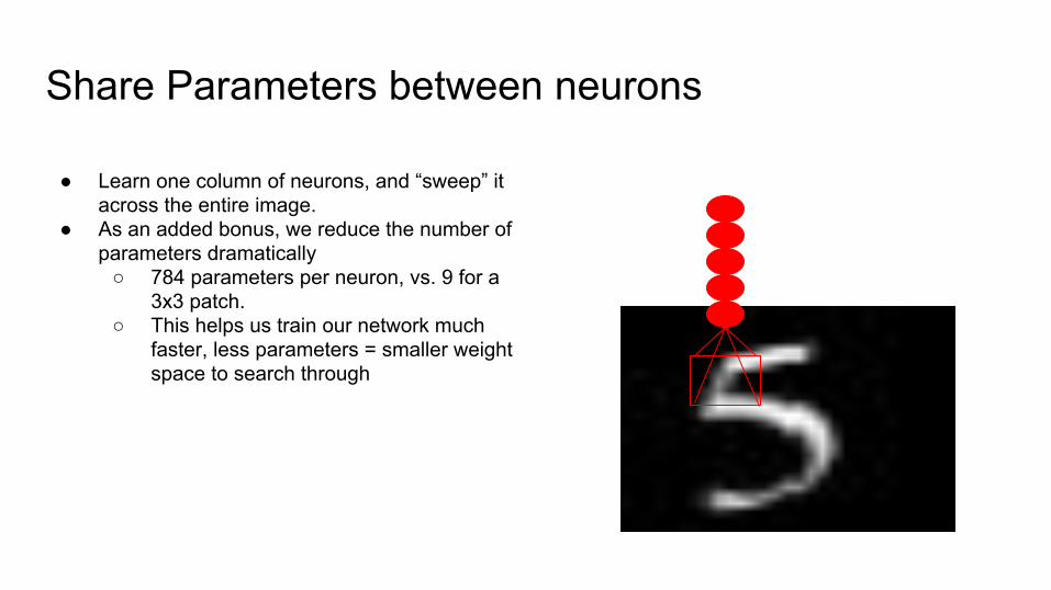
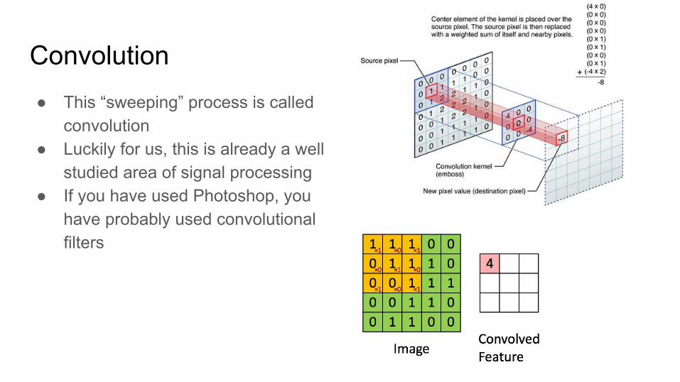
Convolution● This “sweeping” process is called

convolution● Luckily for us, this is already a well

studied area of signal processing● If you have used Photoshop, you

have probably used convolutional filters

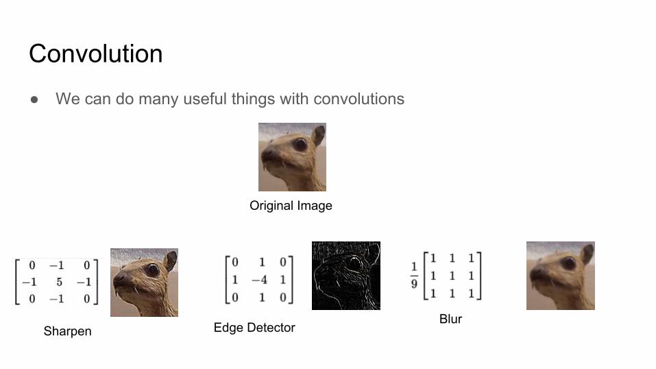
Convolution● We can do many useful things with convolutions

Edge DetectorBlur

Sharpen

Original Image

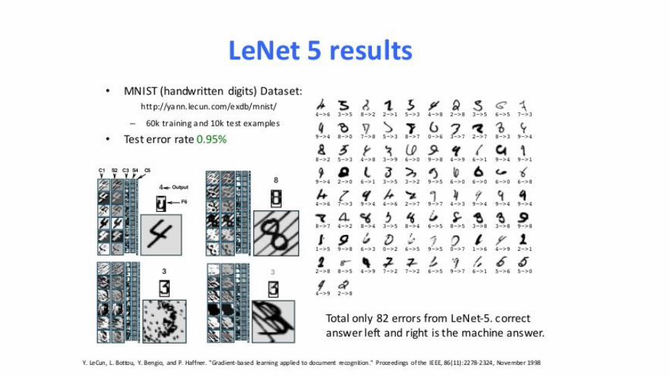
Add More layers - LeNet - Yann LeCun et. All (1989)

● Convolve multiple filters across image.

● Each filter produces a feature map,

○ basically a

filtered version of the image

● Treat feature maps like new images, convolve over them again

● Feature maps are subsampled (typically using max pooling)○ Basically just there to decrease image

size/# of parameters

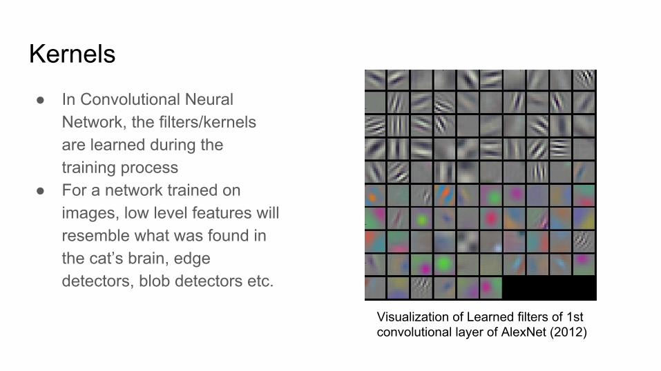
Kernels● In Convolutional Neural

Network, the filters/kernels are learned during the training process

● For a network trained on images, low level features will resemble what was found in the cat’s brain, edge detectors, blob detectors etc.

Visualization of Learned filters of 1st convolutional layer of AlexNet (2012)

Learn a Hierarchy of features

Decompose the Problem into easier problems

PixelsLines/Edges Shapes

Objects

MNIST is kind of simple● MNIST has sanitized data specifically designed as a machine learning

benchmark○ Real world images are messier and more complex

● Linear classifiers can get under 1% error rate with a few tricks + preprocessing

● Lets try something more difficult

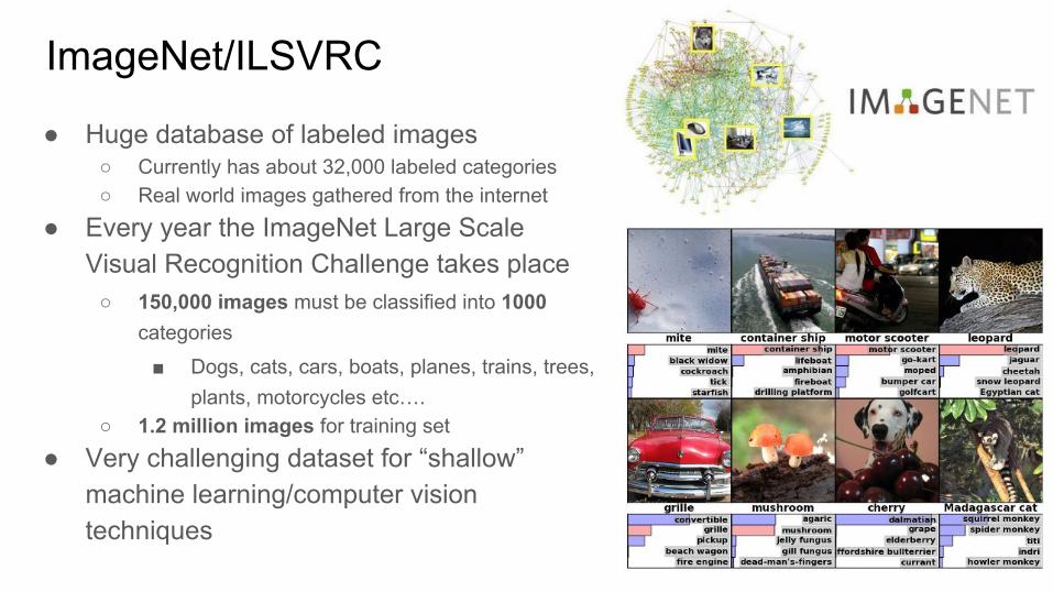
ImageNet/ILSVRC

● Huge database of labeled images○ Currently has about 32,000 labeled categories○ Real world images gathered from the internet

● Every year the ImageNet Large Scale Visual Recognition Challenge takes place

○ 150,000 images must be classified into 1000 categories

■ Dogs, cats, cars, boats, planes, trains, trees, plants, motorcycles etc….

○ 1.2 million images for training set

● Very challenging dataset for “shallow” machine learning/computer vision techniques

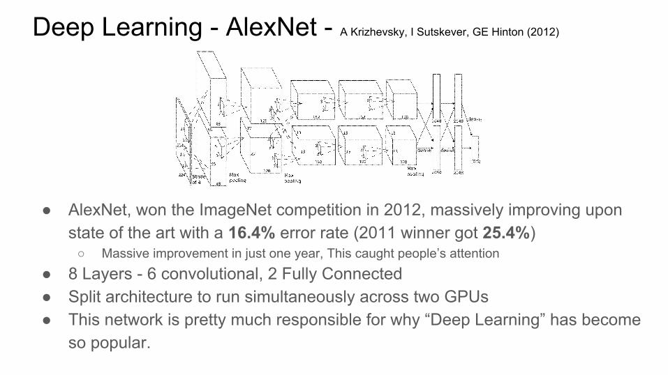
Deep Learning - AlexNet - A Krizhevsky, I Sutskever, GE Hinton (2012)

● AlexNet, won the ImageNet competition in 2012, massively improving upon state of the art with a 16.4% error rate (2011 winner got 25.4%)

○ Massive improvement in just one year, This caught people’s attention

● 8 Layers - 6 convolutional, 2 Fully Connected● Split architecture to run simultaneously across two GPUs● This network is pretty much responsible for why “Deep Learning” has become

so popular.

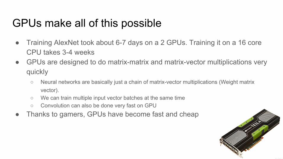
GPUs make all of this possible● Training AlexNet took about 6-7 days on a 2 GPUs. Training it on a 16 core

CPU takes 3-4 weeks● GPUs are designed to do matrix-matrix and matrix-vector multiplications very

quickly○ Neural networks are basically just a chain of matrix-vector multiplications (Weight matrix

vector).○ We can train multiple input vector batches at the same time○ Convolution can also be done very fast on GPU

● Thanks to gamers, GPUs have become fast and cheap

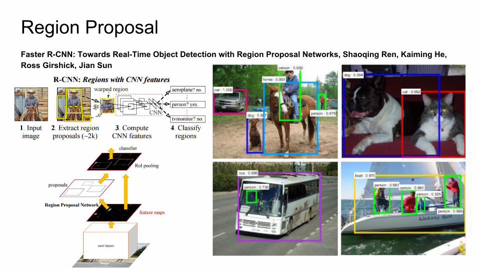
Region ProposalFaster R-CNN: Towards Real-Time Object Detection with Region Proposal Networks, Shaoqing Ren, Kaiming He, Ross Girshick, Jian Sun

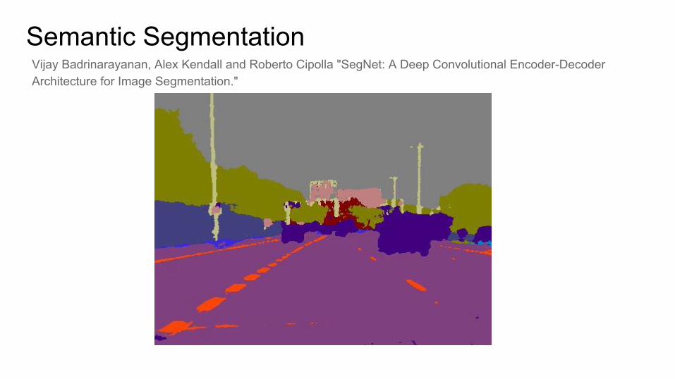
Semantic SegmentationVijay Badrinarayanan, Alex Kendall and Roberto Cipolla "SegNet: A Deep Convolutional Encoder-Decoder Architecture for Image Segmentation."

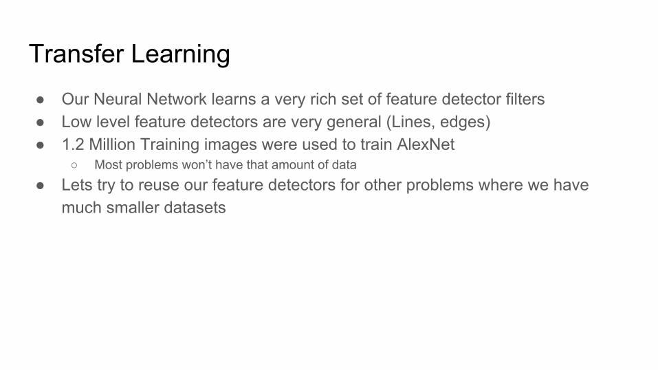
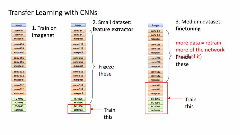
Transfer Learning● Our Neural Network learns a very rich set of feature detector filters● Low level feature detectors are very general (Lines, edges)● 1.2 Million Training images were used to train AlexNet

○ Most problems won’t have that amount of data

● Lets try to reuse our feature detectors for other problems where we have much smaller datasets

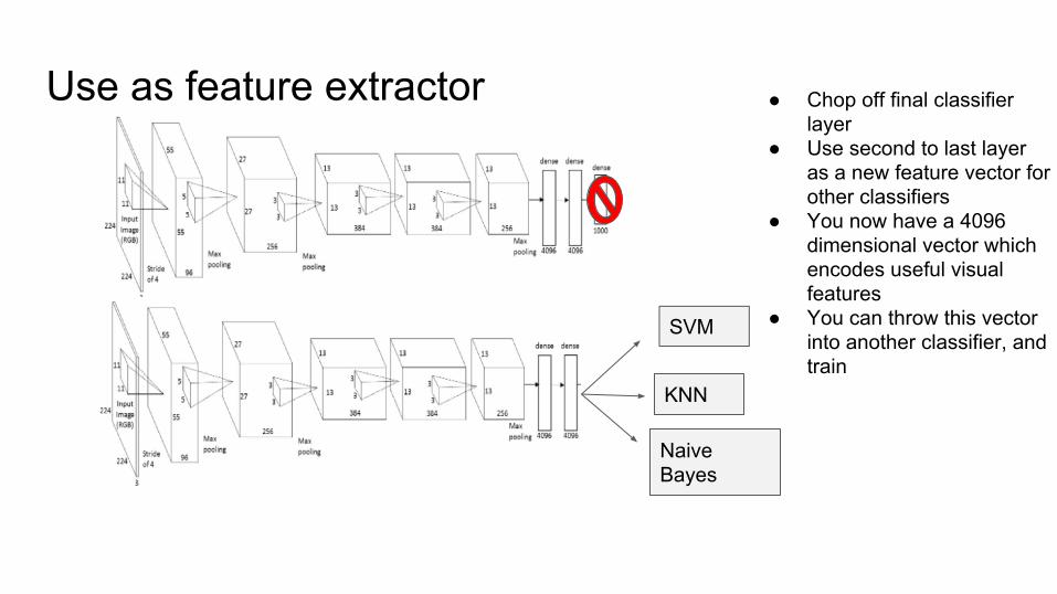
Use as feature extractor ● Chop off final classifier layer

● Use second to last layer as a new feature vector for other classifiers

● You now have a 4096 dimensional vector which encodes useful visual features

● You can throw this vector into another classifier, and train

SVM

KNN

Naive Bayes

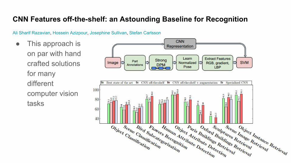
● This approach is on par with hand crafted solutions for many different computer vision tasks

CNN Features off-the-shelf: an Astounding Baseline for Recognition

Ali Sharif Razavian, Hossein Azizpour, Josephine Sullivan, Stefan Carlsson

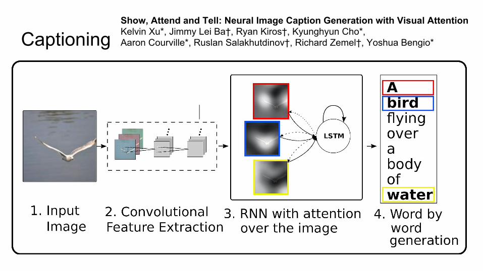
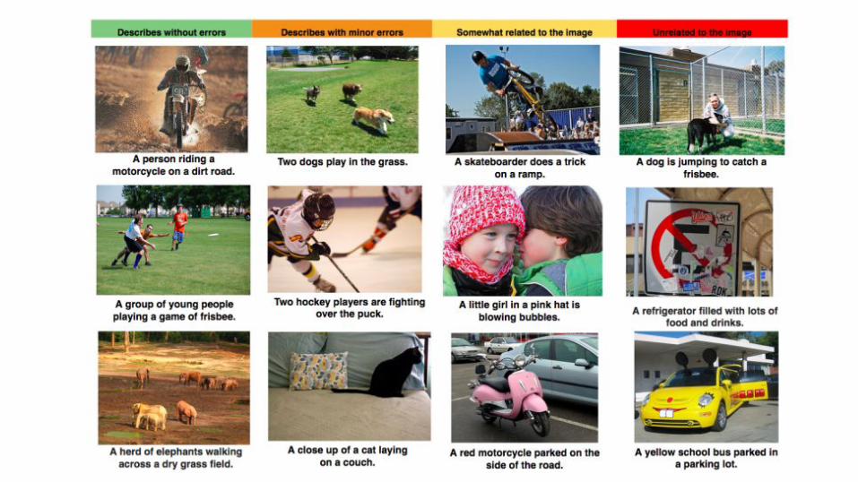
CaptioningShow, Attend and Tell: Neural Image Caption Generation with Visual AttentionKelvin Xu*, Jimmy Lei Ba†, Ryan Kiros†, Kyunghyun Cho*,Aaron Courville*, Ruslan Salakhutdinov†, Richard Zemel†, Yoshua Bengio*

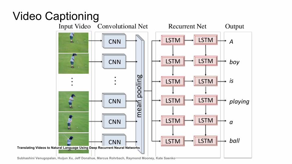
Video Captioning

Translating Videos to Natural Language Using Deep Recurrent Neural Networks

Subhashini Venugopalan, Huijun Xu, Jeff Donahue, Marcus Rohrbach, Raymond Mooney, Kate Saenko

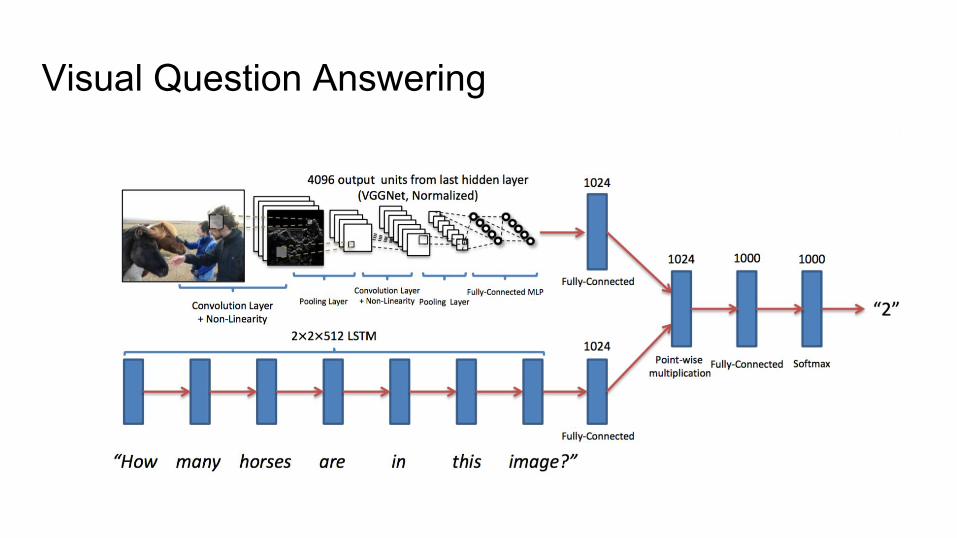
Visual Question Answering

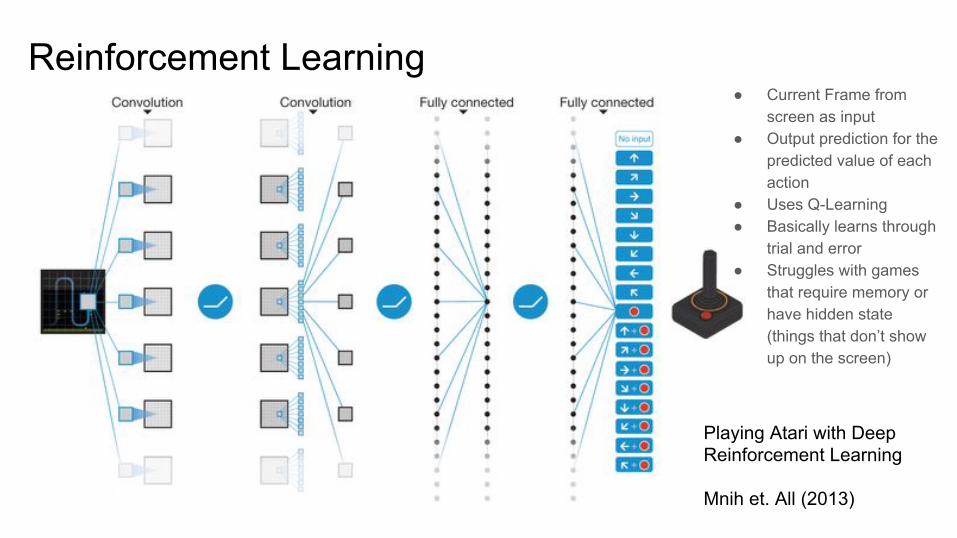
Reinforcement Learning● Current Frame from

screen as input● Output prediction for the

predicted value of each action

● Uses Q-Learning● Basically learns through

trial and error● Struggles with games

that require memory or have hidden state (things that don’t show up on the screen)

Playing Atari with Deep Reinforcement Learning

Mnih et. All (2013)

http://www.youtube.com/watch?v=V1eYniJ0Rnk

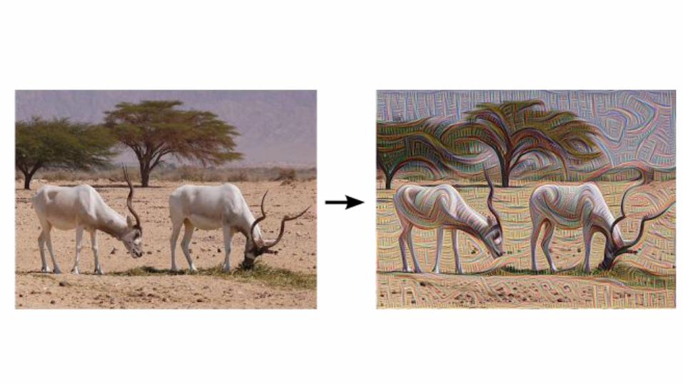
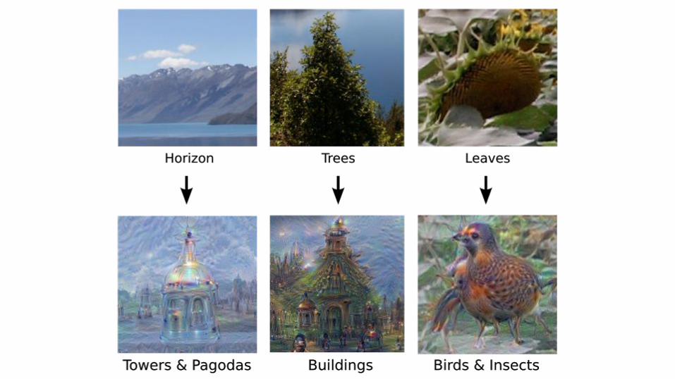
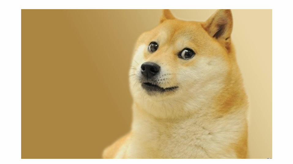
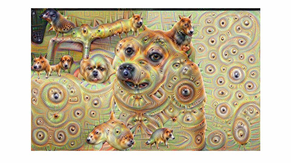
Inceptionism/Deep Dream - How do CNNs “see” things

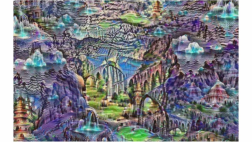
Style Transfer

Keras● Simple and Easy to use Python Library for Deep

Learning● Can run on top of TensorFlow or Theano● Simple, high level code to get the job done

Deeplearning4J● Java Library for Deep learning● Designed for enterprise scale deployment● Good tutorials and Documentation

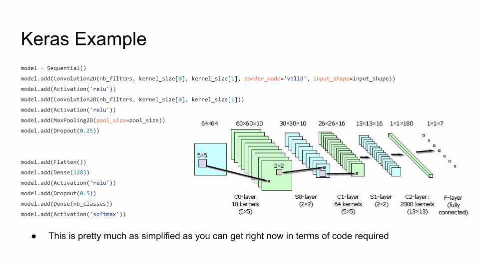
Keras Examplemodel = Sequential()

model.add(Convolution2D(nb_filters, kernel_size[0], kernel_size[1], border_mode='valid', input_shape=input_shape))

model.add(Activation('relu'))

model.add(Convolution2D(nb_filters, kernel_size[0], kernel_size[1]))

model.add(Activation('relu'))

model.add(MaxPooling2D(pool_size=pool_size))

model.add(Dropout(0.25))

model.add(Flatten())

model.add(Dense(128))

model.add(Activation('relu'))

model.add(Dropout(0.5))

model.add(Dense(nb_classes))

model.add(Activation('softmax'))

● This is pretty much as simplified as you can get right now in terms of code required

Libraries

The End

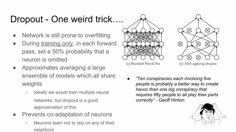
● Network is still prone to overfitting● During training only, in each forward

pass, set a 50% probability that a neuron is omitted

● Approximates averaging a large ensemble of models which all share weights

○ Ideally we would train multiple neural

networks, but dropout is a good approximation of this

● Prevents co-adaptation of neurons○ Neurons learn not to rely on any of their

neighbors

Dropout - One weird trick….

● “Ten conspiracies each involving five people is probably a better way to create havoc than one big conspiracy that requires fifty people to all play their parts correctly” - Geoff Hinton