Convexity Shape Constraints for Image Segmentation

Loic A. Royer1∗ David L. Richmond1∗ Carsten Rother2 Bjoern Andres3 Dagmar Kainmueller1

1MPI-CBG 2TU Dresden 3MPI for Informatics

kainmueller@mpi-cbg.de

Abstract

Segmenting an image into multiple components is a cen-

tral task in computer vision. In many practical scenarios,

prior knowledge about plausible components is available.

Incorporating such prior knowledge into models and algo-

rithms for image segmentation is highly desirable, yet can

be non-trivial. In this work, we introduce a new approach

that allows, for the first time, to constrain some or all compo-

nents of a segmentation to have convex shapes. Specifically,

we extend the Minimum Cost Multicut Problem by a class

of constraints that enforce convexity. To solve instances of

this NP-hard integer linear program to optimality, we sep-

arate the proposed constraints in the branch-and-cut loop

of a state-of-the-art ILP solver. Results on photographs and

micrographs demonstrate the effectiveness of the approach

as well as its advantages over the state-of-the-art heuristic.

1. Introduction

Image segmentation is a challenging task for which often

times the use of suitable prior knowledge about the shape of

the sought objects plays an important role. One interesting

shape prior is convexity [13, 14, 10, 9]. In natural images,

it often occurs that there are multiple convex structures of

the same or different classes present in one image, such

as bricks in walls, floor tiles, and piles of fruit or wooden

logs. Biology similarly gives numerous examples of multiple

convex structures in one micrograph. For example, many

cell types are convex, such as bacteria, yeast, and more

complicated cells densely packed into tissue. Numerous

sub-cellular structures, including nuclei and various types of

vesicles, are also convex. Despite the clear relevance of this

situation to the task of image segmentation, respective priors

have, to the best of our knowledge, not yet been addressed

in the literature.

Existing methods for segmenting multiple convex struc-

tures are specifically designed for certain shapes like ellip-

∗Shared first authors

soids or rods, as e.g. [7]. Such methods do not enforce

generic convexity, but instead employ priors of specific

shapes that happen to be convex. Furthermore, such meth-

ods commonly segment multiple structures sequentially, and

neither the reconstruction of individual structures nor the

resulting segmentation of multiple structures is globally op-

timal w.r.t. the underlying objective.

Beyond specific shape priors, there has been recent inter-

est in generic convexity priors for binary image segmentation.

Star convexity priors were introduced in [14], where convex-

ity is defined with respect to all rays emanating from a cen-

tral, user-defined seed point. This approach was generalized

to the case of Geodesic Star Convexity by [10], which de-

fines convexity with regards to Geodesic paths. Truly convex

objects were first handled by [13]. However, this approach

is limited to a single foreground class, which must be ex-

plicitly modeled. The task of segmenting convex foreground

objects without the requirement of user input or explicit mod-

eling is studied in [9]. They propose a graphical model with

triple-cliques that encode convexity constraints as 1-0-1 label

sequences along straight lines in the image. This formulation

captures the global nature of convexity. However, it implies

that only one connected component of the foreground class

can be present. Furthermore, the complexity of the problem

requires the use of approximate solvers which may lead to

local minima. None of the above methods is able to segment

many generic convex objects of multiple foreground classes,

fully automatically, without user-defined seed points.

Contributions. In this work we propose the first model and

solver for pixel-level segmentation of many generic con-

vex objects of multiple foreground classes. We introduce

new models that include convexity constraints into multicut

problems, which are ILP formulations of image decompo-

sition problems. We consider two multicut problems, one

equivalent to the correlation clustering problem [4], another

one equivalent to the Potts model. For efficiency, follow-

ing the idea in [11, 1], we iteratively incorporate into the

respective ILPs only the constraints that are violated per

instance, and when no more violations occur, we are guar-

anteed the globally optimal solution. To the best of our

knowledge, our models are the first to handle many convex

1402

Figure 1. Method overview. (a) The Multicut Problem (Def. 1) expresses image decomposition as a binary edge labeling problem in a pixel

grid graph. Components are inferred from the edge labels via connectivity analysis. (b) Cycle constraints enforce that edges between pixels

in the same component cannot be cut. (c) We enrich the Multicut Problem by convexity constraints. Our constraints implement the set

theoretic definition of convexity on a discrete grid.

objects and multiple foreground classes. Our models can

be solved to global optimality in small yet practical cases.

Figure 1 gives an overview of the multicut problems as well

as our proposed convexity constraints, as described in detail

in Sections 2 and 3.

2. Image Decomposition by Multicuts

Given the pixel grid graph G = (V,E) of an image,

image segmentation tasks are often modeled as the problem

of assigning, to each node v ∈ V , one label from a label set

L = {1, . . . , k} so as to minimize some objective function.

A widely used objective function is the energy of a pairwise

conditional random field. A particular instance of this type of

objective is the well-known Potts model. Its pairwise terms

are non-zero only for edges that connect nodes with different

labels. A special case of the Potts model is the Correlation

Clustering or Partitioning model [4]. The respective energy

neglects unary terms, and the number of labels equals the

number of nodes.

In the following we describe two Multicut Problems. The

first one is equivalent to Correlation Clustering. The second

one is equivalent to the Potts model. We also discuss respec-

tive solvers as proposed in [11, 1]. These Multicut Problems

are ILPs that form the basis of our contribution: In Section 3

we take the set theoretic definition of convexity of the con-

nected components of a segmentation, and directly translate

it into inequality constraints that we add to the respective

ILPs.

The Minimum Cost Multicut Problem. The minimum

cost multicut problem [6] is equivalent to the correlation

clustering problem. Its feasible solutions are all decompo-

sitions of the graph G. A decomposition of G is a partition

Π of V such that, for every U ∈ Π, the subgraph of Ginduced by U is connected. A subgraph of G that is con-

nected and induced by a node set U ⊆ V is called a com-

ponent of G. Any decomposition Π of G is characterized

by the subset of edges that straddle distinct components:

EΠ = {vw ∈ E | ∀U ∈ Π : v /∈ U ∨ w /∈ U}. Such a sub-

set of edges is called a multicut of G. There is exactly one

multicut related to each decomposition of G. The following

Theorem forms the basis of multicut problems:

Theorem 1 The multicuts of G are precisely the subsets

Y ⊆ E for which every cycle C ⊆ E in G satisfies

|C ∩ Y | 6= 1.

This has been proven in [6]. For a sketch, see Figure 1b.

Let y ∈ {0, 1}E be a 01-encoding of a multicut Y . It

makes explicit, for any pair uv ∈ E of neighboring nodes,

whether u and v are in distinct components, namely iff yuv =1.1 These edge labels ye allow for an equivalent formulation

of |C ∩ Y | 6= 1 as linear inequality constraints (2), which

leads to the following Definition:

Definition 1 [6] Given a finite, simple, non-empty graph

G = (V,E) and a map c : E → R (that is, for any pair

vw ∈ E of neighboring nodes, a cost or reward cvw for

v and w being in distinct components), the instance of the

Minimum Cost Multicut Problem (MC) with respect to Gand c is the ILP

miny∈{0,1}E

∑

e∈E

ceye (1)

subject to

∀C ∈ cycles(G) ∀e ∈ C : ye ≤∑

e′∈C\{e}

ye′ (2)

Constraints (2) are referred to as as cycle constraints. It

is sufficient to consider only the chordless cycles of G [6].

For general graphs, the Minimum Cost Multicut Problem

1Note that in [6] the interpretation of the 01-encoding is flipped, i.e.

ye = 0 means that an edge is an element of the multicut.

403

is NP-hard [4] and APX-hard [8]. For planar graphs, it is

NP-hard and constant-factor approximable [3].

The Minimum Cost Multicut Problem with Node Labels.

We also consider a Multicut Problem that is equivalent to

the Potts model. This is a more constrained optimization

problem in which every node assumes precisely one out of

finitely many labels, and neighboring nodes are in the same

component iff they have the same label:

Definition 2 Given a finite, simple, non-empty graph

G = (V,E), a map c : E → R, a finite set of labels L 6= ∅and a map d : V × L → R (that is, for every node v and

any every l, a cost or reward dvl for v being labeled l), the

instance of the Minimum Cost Multicut Problem with Node

Labels (MCN) with respect to G, L, c and d is the ILP

minx∈{0,1}V ×L

y∈{0,1}E

∑

e∈E

ceye +∑

v∈V

∑

l∈L

dvlxvl (3)

subject to

∀v ∈ V :∑

l∈Lxvl = 1 (4)

∀vw ∈ E ∀{l, l′} ∈(

L2

)

: xvl + xwl′ − 1 ≤ yvw (5)

∀vw ∈ E ∀l ∈ L : yvw ≤ 2− xvl − xwl (6)

Here, any feasible solution (x, y) is constrained such that ev-

ery node v is assigned at least and at most one label, namely

the unique l ∈ L such that xvl = 1, by (4). It is also con-

strained such that, for any edge vw ∈ E, yvw = 1 if and

only if v and w have distinct labels, by (5) and (6). Thus, yis the characteristic function of a multicut of G. It defines

uniquely a decomposition of G.

The MCN (Def. 2) specializes to the MC (Def. 1) for

d ≡ 0 and |L| = |V |, as shown e.g. in [11]. Hence the MCN

is NP-hard.

Solvers. Branch-and-cut algorithms for the MC (Def. 1)

are proposed in [11, 1]. They find globally optimal solutions

in reasonable run-time in many practical cases by includ-

ing constraints (2) per instance of the problem only in case

they are violated. The MCN (Def. 2) is solved by [11] by

transforming it into an equivalent Minimum Cost Multicut

Problem on a modified graph. This transformation involves

flipping the meaning of node label variables resulting in the

so-called multiway cut problem.

3. Method

This Section provides the methodological contribution

of our work. In Section 3.1, we propose a model for image

decomposition under the constraint that each component of

the resulting partition has to be convex. We achieve this

via additional inequality constraints that we include into the

Minimum Cost Multicut Problem (Def. 1). Furthermore,

we propose a respective model with node labels. With this

model, we can enforce for any pair of labels, {k, l} ∈(

L2

)

,

that a component of label k does not contain any node labeled

l in its convex hull. This is more general than “simply”

enforcing convexity of components. We achieve this via

inequality constraints that we include into the Minimum Cost

Multicut Problem with Node Labels (Def. 2). In Section 3.2

we propose a solver for the above optimization problems.

3.1. Convexity Constraints for Image Decomposi­tion

Let P ⊂ E denote an arbitrary open path in G = (V,E).All components of an image decomposition Π are convex

iff for any path P that does not contain any edges in EΠ,

the straight line between the end points of P also does not

contain any edges in EΠ. In other words, for any path P that

lies within a single component, the straight line between its

end points also lies within this component. We discretize

this set theoretic definition of convexity as follows: In a

pixel grid graph with the usual embedding into the 2d plane,

where pixels are Voronoi regions of graph nodes (cf. Fig. 1a),

a component is discrete convex iff for every path P that does

not contain any edges in EΠ, the interior of the loop formed

by P and the straight line between its end points does not

enclose any nodes of a distinct component. We call the set

of nodes enclosed by this loop the hull of P . See Figure 2

for a sketch. Let S(P ) denote the path in G that runs along

the boundary of the discrete hull of P and connects the first

and the last node covered by P (cf. Fig. 2). All components

of an image partition are discrete convex iff

∀P ∈ paths(G) :∑

e∈P

ye = 0 ⇒∑

e∈S(P )

ye = 0. (7)

For a sketch, see Figure 1c. Note that in general, the Bresen-

ham line [5] is different from S(P ), as sketched in Figure 2.

We propose to formulate (7) as linear inequality constraints,

which enables us to formulate the task of finding the optimal

decomposition of G into convex components as an ILP:

Definition 3 Given a finite, simple, non-empty graph

G = (V,E) and a map c : E → R, the instance of the Mini-

mum Cost Convex Component Multicut Problem (Convex-

MC) with respect to G and c is the ILP

miny∈{0,1}E

∑

e∈E

ceye subject to (2) (8)

and

∀P ∈ paths(G) : |S(P )| ·∑

e∈P

ye ≥∑

e∈S(P )

ye (9)

Lemma 1 Constraints (9) are equivalent to (7).

A proof of Lemma 1, as well as a discussion of the computa-

tional complexity of Convex-MC, is given in the Appendix.

We also refer to the Convex-MC as correlation clustering

404

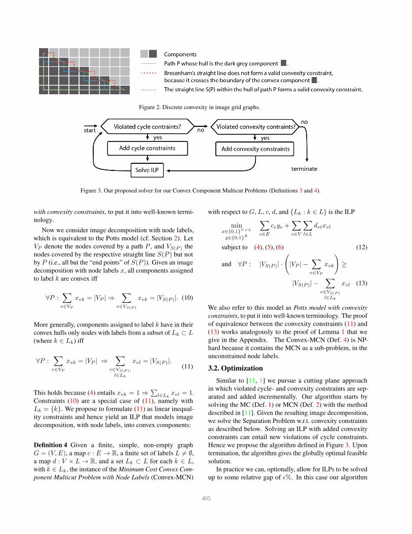
Figure 2. Discrete convexity in image grid graphs.

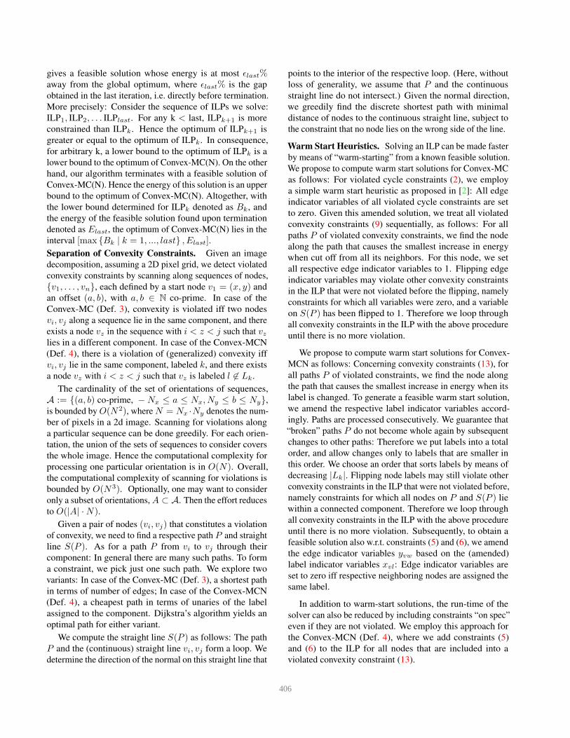
Figure 3. Our proposed solver for our Convex Component Multicut Problems (Definitions 3 and 4).

with convexity constraints, to put it into well-known termi-

nology.

Now we consider image decomposition with node labels,

which is equivalent to the Potts model (cf. Section 2). Let

VP denote the nodes covered by a path P , and VS(P ) the

nodes covered by the respective straight line S(P ) but not

by P (i.e., all but the “end points” of S(P )). Given an image

decomposition with node labels x, all components assigned

to label k are convex iff

∀P :∑

v∈VP

xvk = |VP | ⇒∑

v∈VS(P )

xvk = |VS(P )|. (10)

More generally, components assigned to label k have in their

convex hulls only nodes with labels from a subset of Lk ⊂ L(where k ∈ Lk) iff

∀P :∑

v∈VP

xvk = |VP | ⇒∑

v∈VS(P ),

l∈Lk

xvl = |VS(P )|.(11)

This holds because (4) entails xvk = 1 ⇒∑

l∈Lkxvl = 1.

Constraints (10) are a special case of (11), namely with

Lk = {k}. We propose to formulate (11) as linear inequal-

ity constraints and hence yield an ILP that models image

decomposition, with node labels, into convex components:

Definition 4 Given a finite, simple, non-empty graph

G = (V,E), a map c : E → R, a finite set of labels L 6= ∅,

a map d : V × L → R, and a set Lk ⊂ L for each k ∈ L,

with k ∈ Lk, the instance of the Minimum Cost Convex Com-

ponent Multicut Problem with Node Labels (Convex-MCN)

with respect to G, L, c, d, and {Lk : k ∈ L} is the ILP

minx∈{0,1}V ×L

y∈{0,1}E

∑

e∈E

ceye +∑

v∈V

∑

l∈L

dvlxvl

subject to (4), (5), (6) (12)

and ∀P : |VS(P )| ·

(

|VP | −∑

v∈VP

xvk

)

≥

|VS(P )| −∑

v∈VS(P )

l∈Lk

xvl (13)

We also refer to this model as Potts model with convexity

constraints, to put it into well-known terminology. The proof

of equivalence between the convexity constraints (11) and

(13) works analogously to the proof of Lemma 1 that we

give in the Appendix. The Convex-MCN (Def. 4) is NP-

hard because it contains the MCN as a sub-problem, in the

unconstrained node labels.

3.2. Optimization

Similar to [11, 1] we pursue a cutting plane approach

in which violated cycle- and convexity constraints are sep-

arated and added incrementally. Our algorithm starts by

solving the MC (Def. 1) or MCN (Def. 2) with the method

described in [11]. Given the resulting image decomposition,

we solve the Separation Problem w.r.t. convexity constraints

as described below. Solving an ILP with added convexity

constraints can entail new violations of cycle constraints.

Hence we propose the algorithm defined in Figure 3. Upon

termination, the algorithm gives the globally optimal feasible

solution.

In practice we can, optionally, allow for ILPs to be solved

up to some relative gap of ǫ%. In this case our algorithm

405

gives a feasible solution whose energy is at most ǫlast%away from the global optimum, where ǫlast% is the gap

obtained in the last iteration, i.e. directly before termination.

More precisely: Consider the sequence of ILPs we solve:

ILP1, ILP2, . . . ILPlast. For any k < last, ILPk+1 is more

constrained than ILPk. Hence the optimum of ILPk+1 is

greater or equal to the optimum of ILPk. In consequence,

for arbitrary k, a lower bound to the optimum of ILPk is a

lower bound to the optimum of Convex-MC(N). On the other

hand, our algorithm terminates with a feasible solution of

Convex-MC(N). Hence the energy of this solution is an upper

bound to the optimum of Convex-MC(N). Altogether, with

the lower bound determined for ILPk denoted as Bk, and

the energy of the feasible solution found upon termination

denoted as Elast, the optimum of Convex-MC(N) lies in the

interval [max {Bk | k = 1, ..., last} , Elast].

Separation of Convexity Constraints. Given an image

decomposition, assuming a 2D pixel grid, we detect violated

convexity constraints by scanning along sequences of nodes,

{v1, . . . , vn}, each defined by a start node v1 = (x, y) and

an offset (a, b), with a, b ∈ N co-prime. In case of the

Convex-MC (Def. 3), convexity is violated iff two nodes

vi, vj along a sequence lie in the same component, and there

exists a node vz in the sequence with i < z < j such that vzlies in a different component. In case of the Convex-MCN

(Def. 4), there is a violation of (generalized) convexity iff

vi, vj lie in the same component, labeled k, and there exists

a node vz with i < z < j such that vz is labeled l 6∈ Lk.

The cardinality of the set of orientations of sequences,

A := {(a, b) co-prime, −Nx ≤ a ≤ Nx, Ny ≤ b ≤ Ny},

is bounded by O(N2), where N = Nx ·Ny denotes the num-

ber of pixels in a 2d image. Scanning for violations along

a particular sequence can be done greedily. For each orien-

tation, the union of the sets of sequences to consider covers

the whole image. Hence the computational complexity for

processing one particular orientation is in O(N). Overall,

the computational complexity of scanning for violations is

bounded by O(N3). Optionally, one may want to consider

only a subset of orientations, A ⊂ A. Then the effort reduces

to O(|A| ·N).

Given a pair of nodes (vi, vj) that constitutes a violation

of convexity, we need to find a respective path P and straight

line S(P ). As for a path P from vi to vj through their

component: In general there are many such paths. To form

a constraint, we pick just one such path. We explore two

variants: In case of the Convex-MC (Def. 3), a shortest path

in terms of number of edges; In case of the Convex-MCN

(Def. 4), a cheapest path in terms of unaries of the label

assigned to the component. Dijkstra’s algorithm yields an

optimal path for either variant.

We compute the straight line S(P ) as follows: The path

P and the (continuous) straight line vi, vj form a loop. We

determine the direction of the normal on this straight line that

points to the interior of the respective loop. (Here, without

loss of generality, we assume that P and the continuous

straight line do not intersect.) Given the normal direction,

we greedily find the discrete shortest path with minimal

distance of nodes to the continuous straight line, subject to

the constraint that no node lies on the wrong side of the line.

Warm Start Heuristics. Solving an ILP can be made faster

by means of “warm-starting” from a known feasible solution.

We propose to compute warm start solutions for Convex-MC

as follows: For violated cycle constraints (2), we employ

a simple warm start heuristic as proposed in [2]: All edge

indicator variables of all violated cycle constraints are set

to zero. Given this amended solution, we treat all violated

convexity constraints (9) sequentially, as follows: For all

paths P of violated convexity constraints, we find the node

along the path that causes the smallest increase in energy

when cut off from all its neighbors. For this node, we set

all respective edge indicator variables to 1. Flipping edge

indicator variables may violate other convexity constraints

in the ILP that were not violated before the flipping, namely

constraints for which all variables were zero, and a variable

on S(P ) has been flipped to 1. Therefore we loop through

all convexity constraints in the ILP with the above procedure

until there is no more violation.

We propose to compute warm start solutions for Convex-

MCN as follows: Concerning convexity constraints (13), for

all paths P of violated constraints, we find the node along

the path that causes the smallest increase in energy when its

label is changed. To generate a feasible warm start solution,

we amend the respective label indicator variables accord-

ingly. Paths are processed consecutively. We guarantee that

“broken” paths P do not become whole again by subsequent

changes to other paths: Therefore we put labels into a total

order, and allow changes only to labels that are smaller in

this order. We choose an order that sorts labels by means of

decreasing |Lk|. Flipping node labels may still violate other

convexity constraints in the ILP that were not violated before,

namely constraints for which all nodes on P and S(P ) lie

within a connected component. Therefore we loop through

all convexity constraints in the ILP with the above procedure

until there is no more violation. Subsequently, to obtain a

feasible solution also w.r.t. constraints (5) and (6), we amend

the edge indicator variables yvw based on the (amended)

label indicator variables xvl: Edge indicator variables are

set to zero iff respective neighboring nodes are assigned the

same label.

In addition to warm-start solutions, the run-time of the

solver can also be reduced by including constraints “on spec”

even if they are not violated. We employ this approach for

the Convex-MCN (Def. 4), where we add constraints (5)

and (6) to the ILP for all nodes that are included into a

violated convexity constraint (13).

406

(a) (b)

Figure 4. Examples for convexity constraints in two-label Potts

models. Top row: Photograph of a pile of wooden beams (a),

and micrograph of densely packed cells in a fly wing (b). Mid-

dle row: Two-label Potts model. Bottom row: Convexity constraints

on foreground label of the respective Potts model.

4. Results and Discussion

We present proof-of-concept results of our method on ex-

emplary photographs and biological images. We also show

the respective results obtained without convexity constraints.

We provide a comparison to state of the art [9] on two ex-

emplary images. We employ a four-connected grid graph in

all experiments, check violations of convexity in all discrete

directions, and set the stopping criterion for the ILP solver

to a relative gap of 2%.

Potts Model. Figure 4 shows examples to which we apply

two-label Potts models enriched by convexity constraints on

the foreground label by means of the Convex-MCN (Def. 4).

Figure 4(a) shows a photograph of a pile of wooden beams.

Convexity constraints allow for a perfect segmentation of

the beams. In contrast, a Potts model without convexity

constraints fails to split apart the beams. Figure 4(b) shows

a biological image of polygonal cells in a fly wing. Again,

(a) (b)

Figure 5. Examples for convexity constraints in three-label Potts

models. (a) Photograph of two fried eggs in a pan. Middle: Three-

label Potts model. Bottom: Convexity constraints on yolk label of

the same three-label Potts model. (b) Image of an apple occluding

an orange. Middle: Three-label Potts model. Bottom: Generalized

convexity constraints, with Lapple = {apple} and Lorange =

{apple, orange}. Thus the apple label cannot have anything but

apple in it’s convex hull, while the orange label is allowed to have

apple in it’s convex hull, but not background.

convexity constraints allow for a perfect segmentation of

the cells, while a respective Potts model without convexity

constraints fails to split them apart. Figure 5(a) shows a

photograph to which we apply a three-label Potts model with

convexity constraints on one foreground label. Our method

is able to accurately segment two convex foreground objects

on top of a second, non-convex foreground label.

Results in Figures 4 and 5(a) were achieved with “simple”

convexity constraints as captured by (10). An example for

the more general constraints (11) is given in Figure 5(b).

Here, we enforce components labeled “apple” to be convex

as such, while we enforce components labeled “orange” to be

convex only w.r.t. the background. In other words, we allow

concavities in orange-labeled components as long as they

are filled exclusively by apple-labeled nodes. Consequently

such concavities appear, and both objects are segmented as

desired. However, note that spurious orange components

fringe the apple.

407

(a) (b)

Figure 6. Examples for convexity constraints in correlation clus-

tering models: (a) Photograph of a stone wall. (b) Densely packed

cells in micrograph of fly wing. (Same image as in Figure 4(b).)

Middle: Correlation clustering model. Bottom: Convexity con-

straints in the respective correlation clustering model.

Correlation Clustering. Figure 6 shows two exemplary

results for correlation clustering enriched by convexity con-

straints by means of the Convex-MC (Def. 3). In both exam-

ples, densely packed objects, namely bricks in a stone wall

and cells in a fly wing, are nicely separated due to convexity

constraints. At the same time, the space between these ob-

jects is tesselated into convex components. Although these

results might not be of direct use as segmentations of the re-

spective objects, they may well serve as convex super-voxels

to be used as input for further processing.

Run-time and Optimality. Table 1 lists the energies, num-

bers of iterations, per-instance gaps, and run-times obtained

for our examples. To evaluate the impact of our warm start

and constraint heuristics, we also state run-times without

warm start, as well as with neither warm start nor constraint

heuristics. Note that the ILP stopping criterion of 2 % is

not a hard stopping criterion, and hence smaller gaps are

achieved per instance.

Warm start heuristics tremendously improve run-times,

making our optimization algorithm up to 16 times faster than

without warm start. Constraint heuristics yield smaller but

still significant improvements of run-times. Run-times as

well as speed-ups highly depend on the particular instance

of the problem. As for any NP-hard problem, there is no

guarantee that our optimization algorithm will terminate in

reasonable time. It appears that our warm start heuristics are

particularly effective in cases where objects have to be split

apart. This is intuitively explained by the fact that we find

feasible warm start solutions by breaking paths of violated

constraints, while never replenishing their respective convex

hulls. The latter may be a direction for further speed-ups

via alternative warm start solutions that “convexify” current

solutions. That said, future speed-ups may also be achieved

by different means, e.g. by identifying independent subsets

of variables of individual ILPs, in the spirit of what has been

proposed for Potts models in [12].

Comparison to State-Of-The-Art. We compare our

method to the state-of-the-art for segmentation with con-

vexity constraints [9] on two exemplary images. The method

of Gorelick et al. [9] is able to handle one single convex

structure of one foreground label, and we chose exemplary

images accordingly (Figure 7). We use the code provided by

the authors. First we study a synthetic image (Figure 7 top).

The method of [9] initializes via the Graph Cuts solution,

yielding a hole in the foreground object. In the process of re-

solving this high energy configuration, the method breaks the

outer boundary of the object and settles to a sub-optimal so-

lution. In contrast, our method is able to obtain the globally

optimal solution. On a biological image (Figure 7 bottom),

we ran [9] with two different initializations, namely the stan-

dard Graph Cut solution, as well as a box that we manually

placed around the sought structure. Both initializations result

in sub-optimal solutions, whereas our method is again able

to obtain a globally optimal solution. However, we note that

the method of [9] is considerably faster than ours.

Use Cases and Limitations. Our method ensures that all

connected components of an image partition or the connected

components of desired labels in a Potts model are convex.

Our method is suitable for application to 2D images that

show 2D scenes (like e.g. piles of objects with a convex cross

section, floor or wall tilings, satellite images of buildings or

agricultural fields), or a slices through 3D scenes (commonly

seen in biological applications). The case of occlusions in

photographic images of 3D scenes cannot be handled by our

method without knowing in advance which object occludes

which. This is currently a limitation of our method.

Furthermore, Convex-MC achieves a convex super-

pixelization of an image. This may serve as a valuable

pre-processing step for applications concerned with the seg-

mentation of composite objects formed by convex parts.

408

Experiment Res E ConvexE # Iter Gap Time NoW NoWC

Wooden beams, 2 label Potts 128x128 30686 30868 45 0.3 % 43 sec 524 sec 559 sec

Fly wing, 2 label Potts 101x101 1014 1156 18 1.97 % 91 sec 221 sec 266 sec

Fried eggs, 3 label Potts 163x137 64562 64632 45 0.05 % 36 sec 601 sec 665 sec

Apple and orange, 3 label Potts 100x83 41308 41381 156 0.15 % 1197 sec * *

Stone wall, correlation clustering 101x101 -215 -177 50 1.7 % 28224 sec * -

Fly wing, correlation clustering 101x101 -445 -435 25 0.08 % 66 sec 123 sec -

Table 1. For each experiment, we list the image resolution in pixels (Res), the energy of the solution obtained without convexity constraints

(E), the energy of the solution obtained with convexity constraints (ConvexE), the number of times that convexity constraints are iteratively

added to the ILP (# Iter), the gap achieved in the final iteration (Gap), the run-time of the algorithm with convexity constraints (Time), the

run-time without the described warm-start heuristics (NoW), and with neither warm start nor additional “on-spec” constraints (NoWC).

*Computation omitted due to excessive run times.

(a) (b) (c) (d) (e)

Figure 7. Comparison of our method to the state-of-the-art method of Gorelick et al. [9] on a synthetic and a biological image. Top row:

(a) Synthetic image. (b) Optimal solution of a Potts model. (c,d) Method [9], initialized by (b). (c) First iteration, and (d) sixth iteration

(converged), with energy. (e) Our method obtains the globally optimal convex solution. Bottom: (a) Micrograph of the nucleus of a cell.

(b) Optimal solution of a Potts model. (c) Solution of [9], initialized by (b), and (d) initialized by a square manually placed around the

sought structure (top right small image). Both solutions of [9] are sub-optimal. (e) Our method yields a globally optimal convex solution.

5. Conclusion and Future Work

We proposed a new approach that introduces convexity

constraints into two multicut problems that are equivalent

to Correlation Clustering and the Potts Model, respectively.

Our approach is, to our knowledge, the first that handles

convexity constraints for many connected components of

multiple different classes, and additionally for pre-specified

convexity relationships between objects of different classes.

We have presented proof-of-concept results on exemplary

photographs and micrographs. All concepts described in this

paper extend in a straightforward way to 3D. In future work

we will explore strategies for further improving the run-time

for the application to larger data.

Appendix

Proof of Lemma 1. Given a path P . In case∑

e∈P ye = 0it follows from ye ≥ 0 that (9) ⇔

∑

e∈S(P ) ye ≤ 0 ⇔∑

e∈S(P ) ye = 0 ⇔ (7). Case∑

e∈P ye 6= 0 entails

∑

e∈P ye ≥ 1 because ye ∈ {0, 1}. Hence |S(P )| ·∑

e∈P ye ≥ |S(P )|. And, |S(P )| ≥∑

e∈S(P ) ye because

ye ≤ 1. So, true ⇔ (9) ⇔ (7).

Computational Complexity of Convex-MC. It is, to our

knowledge, an open question whether the Convex-MC (Def.

3) is NP-hard. For initiating a discussion, we offer here a

plausibility argument that leads us to speculate that it might

be hard: The MC (Def. 1) is “almost” polynomially reducible

to Convex-MC: MC and Convex-MC, resp., can be stated

equivalently as a node labeling problem, an unconstrained

integer QP that is invariant under any permutation of labels.

Now, in order to state an instance of the MC as an instance

of the Convex-MC, replace each label in the QP formulation

of the MC with sufficiently many labels, so as to allow for

a decomposition of any non-convex component into convex

components in polynomial time. The only reason why this

construction is not a reduction of MC to Convex-MC is that

the resulting QP, if its solutions are to coincide with those of

the MC, cannot be invariant under all permutations of labels.

409

References

[1] B. Andres, J. Kappes, T. Beier, U. Kothe, and F. Hamprecht.

Probabilistic image segmentation with closedness constraints.

In Computer Vision (ICCV), 2011 IEEE International Confer-

ence on, pages 2611–2618, Nov 2011. 1, 2, 3, 4

[2] B. Andres, T. Kroeger, K. L. Briggman, W. Denk, N. Korogod,

G. Knott, U. Koethe, and F. A. Hamprecht. Globally optimal

closed-surface segmentation for connectomics. In Computer

Vision–ECCV 2012, pages 778–791. Springer, 2012. 5

[3] Y. Bachrach, P. Kohli, V. Kolmogorov, and M. Zadimoghad-

dam. Optimal coalition structure generation in cooperative

graph games. In AAAI, 2013. 3

[4] N. Bansal, A. Blum, and S. Chawla. Correlation clustering.

Machine Learning, 56(1-3):89–113, 2004. 1, 2, 3

[5] J. E. Bresenham. Algorithm for computer control of a digital

plotter. IBM Systems journal, 4(1):25–30, 1965. 3

[6] S. Chopra and M. R. Rao. The partition problem. Mathemati-

cal Programming, 59(1-3):87–115, 1993. 2

[7] R. Delgado-Gonzalo, P. Thevenaz, C. S. Seelamantula, and

M. Unser. Snakes with an ellipse-reproducing property. Image

Processing, IEEE Transactions on, 21(3):1258–1271, 2012.

1

[8] E. D. Demaine, D. Emanuel, A. Fiat, and N. Immorlica. Cor-

relation clustering in general weighted graphs. Theoretical

Computer Science, 361(2):172–187, 2006. 3

[9] L. Gorelick, O. Veksler, Y. Boykov, and C. Nieuwenhuis.

Convexity shape prior for segmentation. In D. Fleet, T. Pajdla,

B. Schiele, and T. Tuytelaars, editors, Computer Vision ECCV

2014, volume 8693 of Lecture Notes in Computer Science,

pages 675–690. Springer International Publishing, 2014. 1, 6,

7, 8

[10] V. Gulshan, C. Rother, A. Criminisi, A. Blake, and A. Zisser-

man. Geodesic star convexity for interactive image segmenta-

tion. In Computer Vision and Pattern Recognition (CVPR),

2010 IEEE Conference on, pages 3129–3136, June 2010. 1

[11] J. Kappes, M. Speth, B. Andres, G. Reinelt, and C. Schnorr.

Globally optimal image partitioning by multicuts. In

Y. Boykov, F. Kahl, V. Lempitsky, and F. Schmidt, editors,

Energy Minimization Methods in Computer Vision and Pat-

tern Recognition, volume 6819 of Lecture Notes in Computer

Science, pages 31–44. Springer Berlin Heidelberg, 2011. 1, 2,

3, 4

[12] J. H. Kappes, M. Speth, G. Reinelt, and C. Schnorr. To-

wards efficient and exact map-inference for large scale dis-

crete computer vision problems via combinatorial optimiza-

tion. In Computer Vision and Pattern Recognition (CVPR),

2013 IEEE Conference on, pages 1752–1758. IEEE, 2013. 7

[13] E. Strekalovskiy and D. Cremers. Generalized ordering con-

straints for multilabel optimization. International Conference

on Computer Vision (ICCV), 2011. 1

[14] O. Veksler. Star Shape Prior for Graph-Cut Image Segmen-

tation. In Computer Vision–ECCV 2008, pages 454–467.

Springer Berlin Heidelberg, Berlin, Heidelberg, 2008. 1

410