ED Convexity Adjustment

8/2/2019 ED Convexity Adjustment

http://slidepdf.com/reader/full/ed-convexity-adjustment 1/19

EURODOLLAR FUTURES CONVEXITY ADJUSTMENTS IN STOCHASTIC

VOLATILITY MODELS

VLADIMIR V. PITERBARG AND MARCO A. RENEDO

A. A formula that explicitly incorporates volatility smile, as well as a realistic correlation structureof forward rates, in computing Eurodollar futures convexity adjustments is derived. The eff ect of volatilitysmile on convexity adjustments is studied and is found significant.

1. I

An interest rate term curve (a collection of discount factors for all future dates) is the fundamental inputfor interest rate derivatives valuation. A term curve is created from (or fit to) prices of liquidly-traded

interest rate instruments. One of the most liquid interest rate contracts is the Eurodollar futures (or ED )contract (and its Euro and Yen equivalents). These are futures contracts with the underlying being a Liborrate, and they are traded on the Chicago Mercantile Exchange (their equivalents are traded on CME, SIMEXand LIFFE). ED futures contracts are fundamental building blocks of interest rate term curves.

The ED contract is subject to margining1. Its price not only incorporates information on the relevantforward rate (the input necessary for building an interest rate term curve), but also on what is known asa convexity adjustment . The convexity adjustment is the extra value that a futures contract on a rate hasover a forward contract on the same rate, arising from the fact that the profits can be reinvested daily at ahigher rate, while the losses can be financed at a lower rate. The value assigned to the convexity adjustmentis model-dependent, that is, it depends on a model of future evolution of interest rates. In order to estimatethe relevant forward rate for a given period from the ED contract price, this convexity adjustment needs tobe estimated first.

In this paper we present a new formula for computing convexity adjustments. It is diff erent from what has

been proposed previously (see Section 2) in a number of important ways. The most fundamental diff erence isthat our formula incorporates the volatility smile, unlike any other formula proposed to date. We demonstratethat accounting for volatility smile properly is vital to value the convexity adjustment correctly2.

Let us define f (t , T , S ) to be the forward value, at time t, of a simple rate covering the period [T, S ] , with0 ≤ t ≤ T < S ; that is,

f (t , T , S ) =P (t, T )− P (t, S )

(S − T ) P (t, S ),

where P (·, ·) are zero-coupon discount factors. As well-known, the value of a futures contract on an assetequals the expected value of its payoff under the risk neutral measure. In particular, the value at time t of the futures contract on the rate f (·, T , S ) is given by (as in [HK00])

F (t , T , S ) = EQt f (T , T , S ) ,(1.1)

where Q is the risk-neutral measure.The convexity adjustment is defined as the diff erence between the futures and the forward on the rate,

Etf (T , T , S )− f (t , T , S ) .

Date : February 04, 2004.Key words and phrases. Eurodollar convexity adjustment, stochastic volatility, volatility smile, forward Libor models.We would like to thank Leif Andersen for his insightful comments.1Marginning is the process of closing a contract at a certain price and writing a similar contract at a new price using a

margin account to pay the diff erence between the two.2This fact has been recognized for other types of convexity adjustments such as constant maturity swap and Libor-in-arrears

convexity adjustments some time ago, but not for ED convexity adjustment.

1



2 VLADIMIR V. PITERBARG AND M ARCO A. RENEDO

Thus, conceptually, computing the convexity adjustment should be as simple as evaluating (1.1) using aMonte-Carlo simulation in an interest rate model of choice. This is, however, unfeasible in practice due tospeed constraints. We address this issue by deriving a closed-form approximation to the “true” model valueof the convexity adjustment, an approximation that is very accurate and fast to compute.

For the same practical reasons, the formula for convexity adjustments should depend on observable marketinputs in the most direct way possible, with lengthy model and curve calibrations reduced to a minimum or

eliminated altogether. In general, as we will demonstrate in the paper, the values of convexity adjustmentsdepend on the law of a joint evolution of a large collection of rates. We reduce this complex dependence toa small number of parameters.

Furthermore, we separate the parameters into two categories: those that change often, and those that donot. The parameters that change, volatility parameters, are taken directly from the prices of options on EDcontracts with diff erent expiries and, importantly, strikes. These parameters can be updated in real time.The other category of parameters, correlation parameters as we call them, come from calibrating a modelwith a rich volatility structure to caps and swaptions. While the latter parameters cannot be updated inreal time, they do not need to be. They can be updated on an infrequent basis and kept constant betweenupdates.

In summary, our formula for ED convexity adjustments,

• Expresses forward rates in terms of futures rates (not the other way around);• Introduces volatility smile as an explicit and direct input;• Is designed for speed of valuation;• Incorporates a sensible correlation structure of rates that can be updated infrequently.

The formula is derived by the following procedure:

1. First, an expansion technique is applied to derive a model-independent relationship that expresses a forward rate as a functional of a collection of futures with expiries on or before the forward rate’sexpiry.

2. Second, the variance terms that appear in the formula are separated into parameters that are easilyobserved in the market and change often (volatility parameters), and those that require calibration tobe estimated but do not change often (correlation parameters).

3. Next, the volatility parameters are represented in a number of ways, both in a model-independent way

as functions of prices of options on ED futures across strikes3, and as closed-form expressions involvingvolatility smile parameters.

4. Finally, the correlation parameters are expressed in terms of the parameters of a forward Libor model(instantaneous Libor volatilities), properly calibrated to relevant market instruments.

Let us comment on the innovative approach used in the first step of the algorithm. Typically an “inverse”procedure is adopted, in which (approximate) values of futures are expressed in terms of forward rates.This still leaves the problem of solving the derived equations to obtain forward rates from market-observedfutures. This step is dispensed with in the algorithm we develop. Moreover, with our approach, it appearsthat significantly more accurate, and model-independent, expansions can be obtained with fewer terms.

In the final stages of preparing this paper, we became aware of the work by Jäckel and Kawai (see [JK04])who also consider the problem of computing Eurodollar convexity adjustments in displaced-lognormal forwardLibor models. While the object of modeling is the same, the diff erences in the approaches and techniquesare significant. Their approximation is derived by formal asymptotic expansions of the drift of a forwardrate in a forward Libor model to an arbitrary order. While we use expansions to the second order only, ourapproach incorporates stochastic volatility and, furthermore, a diff erent quantity is expanded (see previousparagraph). It is also worth reiterating that our main expansion is model-independent.

The paper is concluded with a number of tests. They demonstrate a significant impact that the volatilitysmile has on convexity adjustments, and also verify the accuracy of proposed approximations.

3This is similar to the modern approach for computing constant-maturiy-swap and Libor-in-arrears convexity adjustments,but has not yet been extended to ED convexities.



ED CONVEXITY 3

2. R

There are several published works that address future-forward convexity adjustments, with Flesaker in[Fle93], Burghardt and Hoskings in [BH95], Kirikos and Novak in [KN97], Vaillant in [Vai99], Musiela andRutkowski in [MR97], Hunt and Kennedy in [HK00], and Hull in [Hul02] among them.

The convexity adjustment in [Hul02] is given by the expression 12σ

2t1t2, where σ is the standard deviation

of the short rate in one year, t1 the expiration of the contract, and t2 is the maturity of the Libor rate. Thisformula is an approximation to Flesaker’s formula. Flesaker in [Fle93] derived the convexity adjustment bycomputing the required expectation of a Libor rate under the risk-neutral measure using the Ho-Lee model ina continuous and discrete setup. The formula is extended in [KN97], who derived the convexity adjustmentin the Hull-White model.

Both Ho-Lee and Hull-White models are Gaussian Heath-Jarrow-Morton (HJM) models, ie HJM modelswith deterministic bond (or instantaneous forward rate) volatilities. In such models computing convexityadjustments is straightforward. If the bond price satisfies the SDE

dP (t, T ) = r (t) P (t, T ) dt +Σ (t, T ) P (t, T ) dW (t)

with deterministic Σ (·, ·) , the ED convexity adjustment EQ [f (T , T , S )] − f (0, T , S ) , where f (t , T , S ) is asimple forward rate for period [T, S ] observed at time t, is equal to

1 + (S − T ) f (0, T , S )S − T

e 12

T 0 (Σ(u,S )−Σ(u,T ))2du+1

2

T 0 ((Σ(u,S ))2−(Σ(u,T ))2)du − 1

.

Flesaker’s formula is obtained by setting Σ (t, T ) to −σ(T −t) (Ho-Lee model), and Kirikos-Novak’s formula isobtained by setting Σ (t, T ) to −σ

1− e−κ(T −t)

/κ (Hull-White model). These formulas are fast to compute

but do not incorporate the volatility smile eff ect. Moreover, the Ho-Lee formula and the Hull-White formulaare too simplistic (being one-factor) to capture the de-correlation eff ect on convexity adjustments.

Hunt and Kennedy in [HK00] prove from the first principles that if H is the settlement value of a futurescontract, H is square integrable, and the money market account B(t) is always positive then the martingale

EQt [H ] is a futures price and that the convexity adjustment is given by

cov[H, B(S )]

P (0, S ),

where the covariance is taken under the risk neutral measure. No model-specific calculations are given.Vaillant in [Vai99] proposes a model of the form

dF (t , T , S ) = µ(t)F (t , T , S ) dt + σF (t)F (t , T , S ) dW (t) ,

P (t, S ) = e−(S −t)r(t,S ),

dr (t, S ) = γ (r∞ − r (t, S )) dt + σr(t)r∞ dZ (t) ,

d W (t) , Z (t) = ρ (t) dt,

where W, Z are standard Brownian motions, r (t, S ) is the spot zero rate, and r∞ is some asymptotic valuethe zero rate reaches. The convexity adjustment C (t) = f (t , T , S ) /F (t , T , S ) (defined as the quotientbetween the forward rate and the futures rate) is given by the formula

C (t) = exp−r∞

T t

(S − u)σr(u)σF (u)ρ (u) dt

.

It is not clear whether his model is arbitrage-free and, moreover, no provision is given for the choice of ρ (t),a critical input.

Burghardt and Hoskins in [BH95] analyze the market statistically. They look at the discrete eff ect of mark-to-market and show the existence of the convexity bias empirically. To estimate the convexity bias,they suggest assuming that each forward rate and each zero rate are normally distributed with a givencorrelation, and to linearize the payoff . The convexity adjustment formula they propose consists of two partsreflecting the two simplifications made.

With few notable exceptions (eg the paper [JK04] mentioned in the introduction), the modeling of EDconvexity adjustments has not progressed far beyond simplistic distributional assumptions. In particular, no




model that incorporates a realistic volatility smile has been proposed so far, and no study of the volatilitysmile eff ects on the convexity adjustments has been made. These are the gaps filled by this paper.

3. T

3.1. Preliminaries. Let

0 = T 0 < T 1 < · · · < T N ,

τ n = T n+1 − T n,

be a tenor structure, ie a sequence of (roughly) equidistant dates. We define by P (t, T ) the value, at timet, of a zero coupon bond paying $1 at time T. We define spanning Libor rates

f n (t) f (t, T n, T n+1) =P (t, T n)− P (t, T n+1)

τ nP (t, T n+1),

n = 0, . . . , N − 1.

The numeraire Bt (discretely-compounded money-market account) is defined by

BT 0 = 1,

BT n+1 = BT n × (1 + τ nf n (T n)) , 1 ≤ n < N,Bt = P (t, T n+1) BT n+1 , t ∈ [T n, T n+1] .

The corresponding measure (known as spot Libor measure) is denoted by P. The T n-forward measure (iethe measure for which P (·, T n) is the numeraire) is denoted by Pn.

Let F (t , T , S ) be the value of a futures contract on the rate f (t , T , S ) . We denote F n (t) = F (t, T n, T n+1) ,ie F n (t) is the futures contract on the Libor rate f n (t) .

Proposition 3.1. If the futures contract is marked-to-market only on the dates T 0, T 1, . . . , T N , then its value is given by

F (t , T , S ) = Etf (T , T , S ) .

In particular,

E0f n (T n) = F n (0) .

Proof. See Appendix A.1.

The following relations hold,

F n (0) = E0f n (T n) = E0F n (T n) ,(3.1)

f n (0) = En+10 f n (T n) = En+10 F n (T n) ,(3.2)

for all n. We assume that all F n (0) , n = 0, . . . , N − 1, are known; we would like to derive formulas thatexpress forward rates {f n (0)} in terms of futures {F n (0)} (and other market-observed quantities).

The following result is straightforward.

Proposition 3.2. For each n, n = 1, . . . , N − 1,

f n (0) = E0

ni=0

1 + τ if i (0)

1 + τ if i (T i)

f n (T n)

.(3.3)

This formula expresses the forward rate f n (0) as an expectation of a certain payoff under the spot Libormeasure (not forward measure as in (3.2)), the measure that is used in de fining futures in (3.1). This formulais used as a starting point for deriving expressions for convexity adjustments.

Proof. Follows by measure change.



ED CONVEXITY 5

3.2. Expansion around the futures value. To express the expected value in (3.3) in terms of market-observed quantities, we derive a Taylor series expansion of (3.3) in powers of a small parameter that measuresthe deviation of each of f n (T n) from its mean in the spot Libor measure, F n (0) = E0f n (T n) .

Fix ε > 0, and define f εn’s by

f εn (t) = ε (f n (t)− F n (0)) + F n (0) .

For the future we note that for any n,

f 1n (t) = f n (t) ,(3.4)

f 0n (t) = F n (0) ,(3.5)

∂ f εn (t)

∂ε= f n (t)− F n (0) ,(3.6)

f εn (T n) = ε (f n (T n)−E0f n (T n)) +E0f n (T n) .(3.7)

We define

V (ε) =

n

i=01 + τ if i (0)

1 + τ if εi (T i)

f εn (T n) .(3.8)

It is clear that V (1) is the value on the right-hand side of (3.3),

f n (0) = E0V (1) .(3.9)

Expanding V (ε) into a Taylor series in ε yields,

V (ε) = V (0) +E0∂ V

∂ε(0) × ε +

1

2E0

∂ 2V

∂ε2(0) × ε2 + O

ε3

.(3.10)

The values of the derivatives of V (ε) are computed in the following theorem.

Theorem 3.3. For any n, n = 1, . . . , N − 1,

V (0) = ni=0

1 + τ if i (0)1 + τ iF i (0)

F n (0) ,(3.11)

E0∂ V

∂ε(0) = 0,(3.12)

E0∂ 2V

∂ε2(0) = V (0)

nj,m=0

Dj,m covar (f j (T j) , f m (T m)) ,(3.13)

where the coe ffi cients Dj,m are given by

Dj,m =

−

τ j

1 + τ jF j (0)+ 1{j=n}

1

F n (0)

−

τ m

1 + τ mF m (0)+ 1{m=n}

1

F n (0)

(3.14)

+1{j=m} τ 2

j(1 + τ jF j (0))

2 − 1{j=n}1

F n (0)2

,

and by de fi nition

covar (f j (T j) , f m (T m)) = E0 (f j (T j)−E0f j (T j)) (f m (T m) −E0f m (T m))

= E0 (F j (T j)− F j (0))(F m (T m)− F m (0)) .

The proof is given in the appendix. The main contribution of this theorem is that it expresses quantities

V (0) , E0∂ 2V ∂ε2

(0) from the series expansion (3.10) in terms of quantities that are either directly observable(ie futures and forward rates) or computable (covariances of forward rates). Applying the results of Theorem3.3 to the representation (3.9) and expansion (3.10), the following corollary follows.




Corollary 3.4. For any n, n = 1, . . . , N −1, the (approximation to) forward rate f n (0) can be obtained from

the futures {F i (0)}ni=0 and forward rates for previous periods {f i (0)}n−1

i=0 by solving the following equation,

f n (0) = V (0)

1 +

1

2

nj,m=0

Dj,m covar (f j (T j) , f m (T m))

,(3.15)

with V (0) and Dj,m given in Theorem 3.3.

This corollary provides an algorithm for solving for forward rates f n (0) sequentially for all n, using futuresprices {F j (0)} as inputs.

Remark 3.1. The expression on the right-hand side of (3.15) will be simpli fi ed in the sections that follow.In many cases the rate to be determined from the expression, f n (0) , will appear on the right-hand side of (3.15) as well. In this case, (3.15) should be treated not just as an identity, but as an equation on f n (0).While this may seem to complicate the problem of fi nding f n (0) , in reality the dependence of the right-hand side of (3.15) on f n (0) is typically mild, and the equation can be solved iteratively in just a few steps.

The formula (3.15) depends on covariances between various forward (or futures) rates. These covariancesare not directly observable in the market. We proceed to specify a model that would allow us to relate thisquantity to market observables.

By the definition of the covariance,

covar (f j (T j) , f m (T m)) = (var f j (T j) var f m (T m))1/2 corr(f j (T j) , f m (T m)) ,(3.16)

where the variances and the correlation are computed under the spot Libor measure.

4. C

4.1. Preliminaries. In this section diff erent approaches to computing the variances of forward (or futures)rates, as required by formula (3.16), are proposed. It is the variances of f n (T n) under the spot Libor measurethat are required by the formula. From the modeling prospective, it is much more natural to compute thevariance of each f n (T n) under its own T n+1-forward measure, since each f n (·) is a martingale under itscorresponding forward measure. We propose to approximate var’s in (3.16) with varn+1’s,

varf n (T n) ≈ varn+1 f n (T n) ,(4.1)

n = 1, . . . , N − 1,

where by definition

varn+1 f n (T n) En+10

f n (T n)−En+10 f n (T n)

2.

It can be shown that the error of this approximation is small4. With this approximation, the formula forcomputing forward rates from future ones is expressed as

f n (0) = V (0)

1 +

1

2

nj,m=0

Dj,m

varj+1 f j (T j) varm+1 f m (T m)

1/2corr(f j (T j) , f m (T m))

,(4.2)

4.2. Model-independent approach. A market in options on ED contracts is very liquid, being perhapsthe most liquid market of options on interest rates. The variance of a forward rate can be obtained, ina model-independent way, from the prices of options on the forward rate of diff erent strikes. This is theobservation utilized in this section.

A option on a futures contract expires at the same (or close to) time as the futures contract itself. Since

at expiration F n (T n) = f n (T n) , the option can be regarded as paying (f n (T n)− K )+ at time T n+1. Thevalue of the option at time 0 is given by5

E0B−1T n+1

(f n (T n)− K )+

= P (0, T n+1)En+10 (f n (T n)−K )+

.

4This statement can be made rigorous by showing that the two variances agree to a high order in an expansion with respectto a small volatility scaling parameter. The details are beyond the scope of this paper.

5Options on ED futures are typically American-style. We treat them as Europeans, which should introduce only a smallerror.



ED CONVEXITY 7

Proposition 4.1. The following holds model-independently

varn+1 f n (T n) = En+10

f n (T n)−En+10 f n (T n)

2(4.3)

= 2

f n(0)−∞

En+10 (K − f n (T n))

+dK + 2

∞

f n(0)

En+10 (f n (T n)−K )+

dK.

The proof is standard and is omitted.This method has an advantage in that, to compute variances in (4.2), it directly uses observable option

prices. The forward f n (0) , the rate to solve for, enters the right-hand side of the equation only as anintegration limit in (4.3). The comments of Remark 3.1 apply.

The formula (4.3) demonstrates explicitly one of our main statements, namely that the ED convexityadjustment value depends on prices of options of all strikes, ie on the volatility smile.

The formula (4.3) is intuitive and theoretically appealing, but may not be easy to use in practice. Thisis so because only a discrete set of strikes is typically traded, and not all of them are very liquid. For thesereasons, a model-based approach may be preferable. It is based on computing the required variances of forward rates in a model that is calibrated to the volatility smile in options.

Stochastic volatility models are widely recognized as providing the superior framework for modeling volatil-ity smiles in interest rates, see [AA02]. Moreover, stochastic volatility models typically have intuitive para-

meters and efficient numerical methods for valuation and calibration. While only individual forward ratesneed to be modeled, for reasons that will be clear later, a term structure model will be required. A “global”forward Libor model with stochastic volatility is defined next.

4.3. The forward Libor model with stochastic volatility. A stochastic variance process z (t) is definedby the SDE

dz (t) = θ (z0 − z (t)) dt + η

z (t) dV (t) ,(4.4)

z (0) = z0.

Let

dW (t) = (dW 1 (t) , . . . , d W K (t))

be a K -dimensional Brownian motion (under the measure Q) independent of dV. The Stochastic Volatilityforward Libor model is defined by the following dynamics imposed on the spanning forward Libor rates underthe appropriate forward measures,

df n (t) = (bf n (t) + (1 − b) f n (0))

z (t)K k=1

σk (t; n) dW n+1k (t) ,

n = 1, . . . , N − 1.

The following SDEs govern the dynamics of Libor rates under the spot Libor measure,

df n (t) = (bf n (t) + (1 − b) f n (0))

z (t)

K k=1

σk (t; n)

z (t)µk

t, f̄ (t) ; n

dt + dW k (t)

,(4.5)

n = 1, . . . , N − 1.

Here

µk

t, f̄ (t) ; n

are Libor rate drifts whose form can be found in eg [ABR01].The shape of the volatility smile produced by the model is primarily governed by the blending parameter

b and the volatility of variance parameter η. Blending b aff ects the slope of the volatility smile, while η

aff ects its curvature. The mean reversion of variance parameter θ controls the evolution of the volatilitysmile with time, and the volatility structure σ (·; ·) determines the overall level of volatilities for all capletsand swaptions. They are usually calibrated to match at-the-money volatilities of all swaptions. For moredetails see [Sid00] and [AA02].




4.4. Forward rate variances in the forward Libor model with stochastic volatility. In this section

varn+1 f n (T n) = En+10

f n (T n)−En+1

0 f n (T n)2

is evaluated in the model developed in Section 4.3 (recall that these variances are needed for the mainvaluation formula (4.2)). Let us denote

un (s) =

K k=1

σ2k (s; n)

1/2

.

Proposition 4.2. Denote the moment generating function of T n0

z (s) u2n (s) ds by χn (µ) ,

χn (µ) En+10

exp

µ

T n0

z (s) u2n (s) ds

.

Then

varn+1 f n (T n) =f 2n (0)

b2χn

b2− 1

.

Proof. See Appendix A.3.

Note that the function χn (µ) can be computed by numerically solving a Riccati system of ordinarydiff erential equations, see [AP04]. Also note that f n (0) enters the expression for the variance (and theright-hand side of (4.2) by extension). The equation (4.2) is of degree 2 in f n (0) and can either be solvedexactly, or by iteration as explained in Remark 3.1.

The result of Proposition 4.2 is useful from a theoretical prospective, but is not very helpful in practice,since it requires a fully-calibrated stochastic volatility forward Libor model to compute the variances, amodel that is typically (relatively) slow to calibrate. The result is simplified in the next section.

4.5. Forward rate variances in a simple stochastic volatility model. Rather than using a full-blownforward Libor model, practitioners prefer reduced-form models to value options on ED futures (as well ascaps and swaptions). Since under the appropriate forward measure a forward rate is a martingale, the Black

model can be used, and has historically been the model of choice. Relatively recently, more sophisticatedmodels started to appear. Arguably, the most popular among them is the stochastic volatility model.With the reduced-form model, only a single forward rate at a time is being modeled. For the rate f n (t) ,

the following model can for example be used,

dz (t) = θ (z0 − z (t)) dt + ηn

z (t) dV (t) ,(4.6)

df n (t) = λn (bnf n (t) + (1 − bn) f n (0))

z (t) dU (t) .

These equations can be understood to be under the T n+1-forward measure. The set of parameters (λn, bn, ηn)define the volatility smile in options on the rate f n (T n).

While superficially the model (4.6) appears similar to the model (4.4)-(4.5), the key diff erence is thatin the former each forward rate is modeled separately, while in the latter the joint evolution of rates isconsidered.

The value of the variance in the model (4.6) can be obtained easily.

Proposition 4.3. Denote the moment generating function of λ2n T n0 z (s) ds in the model (4.6) by χ0n (µ) ,

χ0n (µ) En+10

exp

µλ2n

T n0

z (s) ds

.(4.7)

Then

varn+1 f n (T n) =f 2n (0)

b2n

χ0n

b2n− 1

.

Proof. Similar to the proof of Proposition 4.2, see Appendix A.3.



ED CONVEXITY 9

The moment-generating function χ0n (µ) can be written out in closed form, see Appendix B. Moreover,one of the methods of calibration for the stochastic volatility forward Libor model (see [Pit04]) advocatesusing the method of matching moment generating functions χ0n (µ) and χn (µ) for certain values of µ. Thisprovides another connection between Proposition 4.2 and 4.3.

We again comment that the expression for the variance varn+1 f n (T n) involves f n (0) , that would appearon the right-had side of (4.2) and would make it a quadratic equation.

One should realize that the implied values of parameters (λn, bn, ηn) also technically depend on theparameter f n (0) . However, the loss of accuracy is negligeable if (λn, bn, ηn) are implied with the “previous”value of the forward rate f n (0) , ie the value before the update of the convexity adjustment.

As explained in [AP04], the variance varn+1 f n (T n) can become infinite for certain values of parametersof the model (4.6). In practice, a suitable restriction of the domain of integration will solve this problem.

5. C

By direct computation in the forward Libor model (4.5), assuming T j ≤ T m, we obtain,

corr (f j (T j) , f m (T m))

= E0

T j

0

ϕ (f j (s))ϕ (f m (s)) z (s)K

k=1

σk (s; j)σk (s; m) ds

×

E0

T j0

ϕ2 (f j (s)) z (s)K k=1

σ2k (s; j) ds

−1/2

×

E0

T m0

ϕ2 (f m (s)) z (s)K k=1

σ2k (s; m) ds

−1/2.

By “freezing” the forward rates at their initial values when used as arguments in the local volatility functions,a correlation approximation formula6 is obtained,

corr(f j (T j) , f m (T m)) =

T j0

K k=1 σk (s; j)σk (s; m) ds

T j0 K k=1 σ

2k (s; j) ds

1/2

T m0 K k=1 σ

2k (s; m) ds

1/2.(5.1)

Model parametersσ2k (·; m)

are not directly observable; to extract them, the model needs to be cal-

ibrated to market inputs. This is why the power of the fully-calibrated forward Libor model is required.Options on Libor rates (caplets and ED options) do not contain this information; calibrating exclusively tothese options is not sufficient to extract the required correlation information from the market. Thus, the cal-ibration procedure needs to include a wider range of instruments. Fortunately, European swaptions (optionsto enter interest rate swaps) of various expiries and maturities are very liquid. Since European swaptionscan be viewed as options on baskets of Libor rates (see Rebonato’s book [Reb98]), their market-quotedimplied volatilities can be seen to contain Libor rate correlation information. A calibration of the forwardLibor model (see [Sid00]) to caps and swaptions returns

σ2k (·; m)

, from which the required correlations

can be computed with the help of (5.1). In essence, the forward Libor model is used as a “device” to extractimplied Libor rate correlations from the swaption market. (A similar approach is advocated in [And04] forcalibrating a simple interest rate model for pricing Bermudan swaptions.) Since correlations do not change

often, this calibration does not have to be performed intra-day.

6. T

Let us present the final formula that we propose to use. Of the three approaches we developed forcomputing variances, we advocate using the reduced-form stochastic volatility model of Libor rates (Section4.5). The other two approaches, while perhaps theoretically more appealing for the reasons of model-independence (Section 4.2) or consistency with correlation computations (Section 4.4), are not as well-suitedfor practical applications.

6This formula can be interpreted as a leading-term in the expansion of the original formula in a small volatility scalingparameter.



10 VLADIMIR V. PITERBARG AND MARCO A. RENEDO

Before stating the result, let us recall the notations. Let {f n (0)}N n=1 be the (unknown) sequence of forward

rates for the tenor structure {T n}N n=0 . Let {F n (0)}N

−1n=1 be the (known) sequence of futures contracts on these

rates. For each n, n = 1, . . . , N − 1, let the triple (λn, bn, ηn) be the set of parameters of the model (4.6)implied from market prices of options on the rate f n (T n) (options expiring at T n and with diff erent strikes).Finally, let {σk (·; n)}k,n be instantaneous factor volatilities of forward rates as obtained from a calibrated

forward Libor model (4.5).

Theorem 6.1. For each n, n = 1, . . . , N − 1, the forward rate f n (0) can be obtained from the futures

{F i (0)}ni=0 and forward rates for previous periods {f i (0)}n−1

i=0 by solving the following equation,

f n (0) = V (0)

1 +

1

2

nj,m=0

Dj,mf j (0) f m (0)

b2χ0j

b2j− 1

1/2 χ0m

b2j− 1

1/2cjm

,(6.1)

with

V (0) = V (0) =

ni=0

1 + τ if i (0)

1 + τ iF i (0)

F n (0) ,

Dj,m =

−

τ j

1 + τ jF j (0)+ 1{j=n}

1

F n (0)

−

τ m

1 + τ mF m (0)+ 1{m=n}

1

F n (0)

+1{j=m}

τ 2j

(1 + τ jF j (0))2 − 1{j=n}

1

F n (0)2

,

and

cjm =

T j0

K k=1 σk (s; j)σk (s; m) ds

T j0

K k=1 σ

2k (s; j) ds

1/2

T m0

K k=1 σ

2k (s; m) ds

1/2

,(6.2)

χ0n (µ) = En+10

exp

µλ2n

T n

0

z (s) ds

.

The functions χ0n (µ) can be computed in closed form, see Appendix B.

Proof. The proof follows by combining the statement of Corollary 3.4, equations (3.16), (4.1), Proposition4.3 and equation (5.1).

7. T

The formula we have derived for ED convexity adjustments is unique; it is, to the best of our knowledge,the only one that explicitly incorporates volatility smile. Thus, testing it against other “alternatives” is not

very illuminating. Instead, we perform the following studies. First, we look at the eff ects of volatility smileparameters on ED convexity adjustments. Second, we take the Monte-Carlo-computed values of convexityadjustments in a fully-calibrated stochastic volatility forward Libor model as their “true” values, and proceedto test the formula we derived against them. This checks the accuracy of approximations made in derivingthe formula.

In all tests, Eurodollar futures with expiries up to 5 years are considered (Eurodollar futures with expiriesup to 4 years are considered liquid; after four years, they are typically replaced with swaps as primary interestrate curve building instruments). There are 20 contracts in total. The first is assumed to start in 3 monthsfrom the valuation date.

The results are presented in basis points (bp), ie 0.01-ths of a percent. For reference, a bid-ask spread ona typical ED contract is 0.5 basis points.



ED CONVEXITY 11

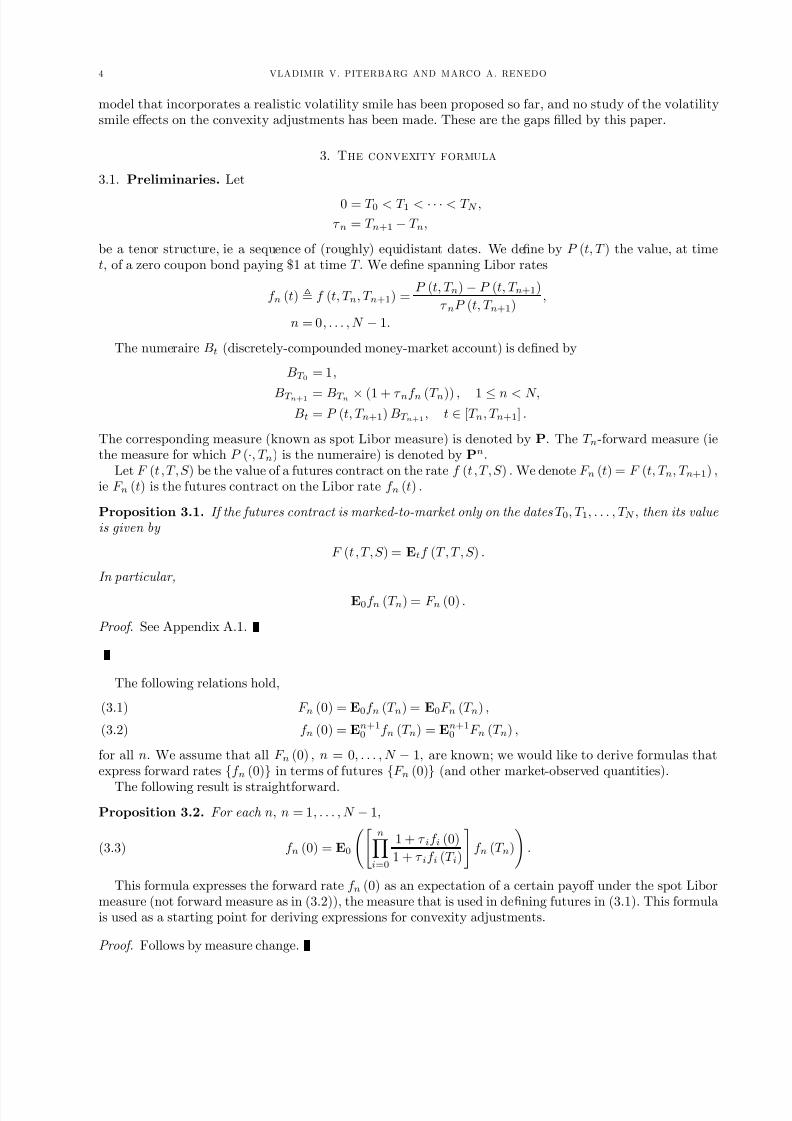
7.1. Eff ect of stochastic volatility parameters on convexity adjustments. The eff ects of stochasticvolatility parameters (blending parameters bn and volatility of variance parameters ηn from Sections 4.4and 4.5) on ED convexity adjustments is studied. The convexity adjustments are computed by the formulafrom Theorem 6.1, with the simple stochastic volatility model (4.6) used to compute the variances. Thecorrelations {cjm} in (6.1) are not taken from a forward Libor model as in (6.2), but specified externally, asexplained below.

To allow for easy reproducibility of our test results, simulated market conditions are considered. Theconditions are chosen to broadly reflect the features of the US interest rate market at the time of writing.The input rates on futures contracts are given by

F n (0) = 0.01 + 0.04 ×T n5

,

n = 1, . . . , 20.

The “market” stochastic volatilities are given by

λn = 0.5 − 0.35 ×T n10

,

n = 1, . . . , 20.

Also,

z0 = 1,

θ = 0.3.

The correlations {cjm} in (6.1) are computed according to the formula

cjm =

1 − exp(−2a min(T j , T m))

1 − exp(−2a max(T j , T m))

1/2

,

a = 0.05,

j, m = 1, . . . , 20,

(this is a formula for correlations between appropriate forward continuously-compounded rates in a simpleone-factor Gaussian model with constant volatility and mean reversion parameter a).

Convexity adjustments F n (0) − f n (0) , n = 1, . . . , 20, are evaluated using the formula (6.1) for variouslevels of blending b and volatility of variance η (flat parameters bn ≡ b, ηn ≡ η are used). In Table 1,convexity adjustments for various contracts (rows) and levels of blending b (columns) are presented. InTable 2, convexity adjustments for various contracts (rows) and volatilities of variance η (columns) arepresented. The results are presented graphically in Figure 1 and Figure 2.

Clearly, the eff ect of blending and volatility of variance on convexity adjustments is very significant. Forback-end contracts (5 years to expiry), the diff erence between the extreme blending values (b = 0.0 andb = 1.0) is about 20 basis points, a huge diff erence. The diff erence is also extremely large, at about 5 basispoints, between the models with η = 0 and η = 100%. Clearly, mis-specifying (or not account for) thevolatility smile parameters has a very pronounced impact on convexity adjustments.

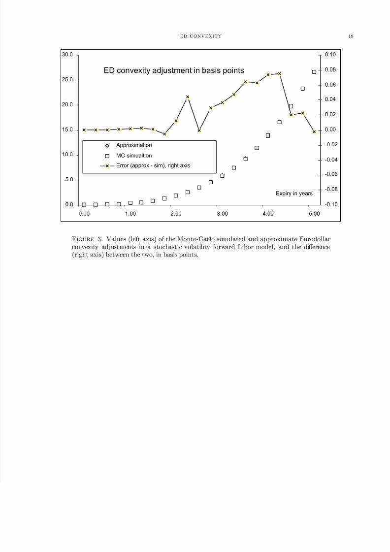
7.2. Formula versus Monte-Carlo. In this section, an interest rate curve and a forward Libor model arespecified, and the approximate formula developed in Theorem 6.1 is compared to the “brute-force” Monte-Carlo simulated values of F n (0) , n = 1, . . . , 20. Monte-Carlo values are computed by averaging over 250,000paths.

An interest rate curve used in testing is given by

P (0, t) = exp

−

t0

φ (s) ds

,

φ (t) = 0.01 + 0.04 ×t

5,

t ≥ 0.




A two-factor forward Libor model is used, with

σ1 (t; n) ≡ 0.2,

σ2 (t; n) = 0.5 × e−0.4t − 0.15.

Stochastic volatility parameters are given by

b = 0.5,η = 0.5,

θ = 0.3,

z0 = 1.

The results are presented in Figure 3. Clearly, the agreement between the “true” model value (computedvia Monte-Carlo) and the approximation (6.1) is very good, within 0.1 basis point for all contracts.

R

[AA02] Leif B.G. Andersen and Jesper Andreasen. Volatile volatilities. Risk , 15(12), December 2002.[ABR01] Leif B.G. Andersen and Rupert Brotherton-Ratcliff e. Extended libor market models with stochastic volatility. Working

paper, 2001.

[And04] Jesper Andreasen. Markov yield curve models for exotic interest rate products. Lecture notes, 2004.[AP04] Leif B.G. Andersen and Vladimir V. Piterbarg. Moment explosions in stochastic volatility models. SSRN working

paper, 2004.[BH95] Galen Burghardt and B. Hoskins. A question of bias. Risk , pages 63—70, March 1995.[Fle93] Bjorn Flesaker. Arbitrage free pricing of interest rate futures and forward contracts. The Journal of Futures Markets ,

13(1):77—91, 1993.[HK00] Philip Hunt and Joanne Kennedy. Financial Derivatives in Theory and Practice . John Wiley and Sons, 2000.[Hul02] John C. Hull. Options, futures and other derivatives . Prentice Hall, 2002.[JK04] Peter Jaeckel and Atsushi Kawai. The future is convex. Working paper, 2004.[KN97] George Kirikos and David Novak. A question of bias. Risk , pages 60—61, March 1997.[MR97] Marek Musiela and Marek Rutkowski. Martingale Methods in Financial Modeling . Springer, 1997.[Pit04] Vladimir V. Piterbarg. A stochastic volatility model with time-dependent skew. To appear in Applied Mathematical

Finance, 2004.[Reb98] Riccardo Rebonato. Interest-Rate Option Models . John Wiley and Son, 1998.[Sid00] Jakob Sidenius. Libor market models in practice. Journal of Computational Finance , 3(Spring):75—99, 2000.

[Vai99] N. Vaillant. Convexity adjustments between futures and forward rate using a martingale approach. Probability tuto-rials, 1999.

A A. P

A.1. Proof of Proposition 3.1. Kennedy and Hunt in [HK00] showed that in the case of discrete margin-ing, futures price F (t , T , S ) for t in [T i, T i+1) is given by

F (t , T , S ) =Et

F (T i+1, T , S ) B−1

T i+1

+Et

nj=i+2 (F (T j , T , S )− F (T j−1, T , S )) B−1

T j

Et

B−1T i+1

.

Assume, by induction, that for all k > i and for all t in [T k, T k+1), Et[f (T , T , S )] = F (t , T , S ). It will be

shown that for all t in [T i, T i+1), Et[f (T , T , S )] = F (t , T , S ).The key to prove the statement is to observe that if Bt is the numeraire of the spot Libor measure, thenBT j is known at time T j−1, for any j. Using this fact and the induction assumption,

Et

nj=i+2

(F (T j , T , S )− F (T j−1, T , S )) B−1T j

= Et

nj=i+2

B−1T jET j−1 [(F (T j, T , S )− F (T j−1, T , S ))]

= 0



ED CONVEXITY 13

By the same property,

Et

F (T i+1, T , S ) B−1

T i+1

Et

B−1T i+1

= Et [F (T i+1, T , S )]

which proves the result.

A.2. Proof of Theorem 3.3. Define

p (y0, . . . , yn) =

ni=0

1

1 + τ iyi

yn.

Then

∂

∂ yj p = −

τ j

1 + τ jyj

ni=0

1

1 + τ iyi

yn + 1j=n

ni=0

1

1 + τ iyi

= p

−

τ j

1 + τ jyj+ 1j=n

1

yn

Also,

∂

∂ ym

∂

∂ yj p =

∂

∂ ym p

−

τ j

1 + τ jyj+ 1j=n

1

yn

(A.1)

+ p

1j=m

τ 2j

(1 + τ jyj)2 − 1m=n1j=n

1

y2n

= p

−

τ m

1 + τ mym+ 1m=n

1

yn

−

τ j

1 + τ jyj+ 1j=n

1

yn

+ p

1j=m

τ 2j

(1 + τ jyj)2 − 1m=n1j=n

1

y2n

.

Recall (3.8),

V (ε) =

ni=0

1 + τ if i (0)

1 + τ if εi (T i)

f εn (T n) .

Clearly

V (ε) =

ni=0

(1 + τ if i (0))

p (f ε0 (T 0) , . . . , f εn (T n)) .

Obviously, (3.11) follows from (3.5). Moreover,

V (ε) =

ni=0

(1 + τ if i (0))

n

j=0

∂

∂ yj p (f ε0 (T 0) , . . . , f εn (T n))

∂ f εj (T j)

∂ε

=

ni=0

(1 + τ if i (0))

nj=0

∂

∂ yj p (f ε0 (T 0) , . . . , f εn (T n)) (f j (t)− F j (0))

(A.2)

where (3.6) was used for the second step. Thus,

V (0) =

ni=0

(1 + τ if i (0))

n

j=0

∂

∂ yj p (F 0 (0) , . . . , F n (0))(f j (t)− F j (0))

.

Since

E0 (f j (t)− F j (0)) = 0,




we obtain

E0V (0) = 0,

ie (3.12) is proved.Diff erentiating (A.2) with respect to ε again, we obtain

V (ε) =

ni=0

(1 + τ if i (0))

j,m

∂ 2

∂ ym∂ yj p (f ε0 (T 0) , . . . , f εn (T n)) (f j (t)− F j (0))(f m (t)− F m (0))

,

and

V (0) =

ni=0

(1 + τ if i (0))

p (F 0 (0) , . . . , F n (0))

j,m

Dj,m (f j (t) − F j (0))(f m (t)− F m (0))

,

where we have used (A.1) and the definition (3.14) of Dj,m’s. Simplifying, we obtain

V

(0) = V (0)

j,mDj,m (f j (t)− F j (0))(f m (t)− F m (0))

.

Taking the expected value E0 from both sides, (3.12) is obtained. This concludes the proof of the theorem.

A.3. Proof of Proposition 4.2. Recall that

un (s) =

K k=1

σ2k (s; n)

1/2

.

Denote

dU n (s) =

1

un (s)

K k=1

σk (s; n) dW

n+1

k (t) .

It is easy to see that dU n (s) is a drift-less Brownian motion under Pn+1.Under Pn+1,

f n (T n) =f n (0)

b

exp

b

T n0

z (s)un (s) dU n (s)−

b2

2

T n0

z (s) u2n (s) ds

− (1− b)

.

Thus

varn+1 f n (T n) =f 2n (0)

b2En+10

exp

b

T n0

z (s)un (s) dBn (s)−

b2

2

T n0

z (s) u2n (s) ds

− 1

2.

Conditioning on z (·) we obtain

varn+1 f n (T n) =f 2n (0)

b2En+10

exp

b2 T n0

z (s) u2n (s) ds

− 1

.

The moment-generating function of T n0 z (s) u2n (s) ds is known (see Appendix B) and is easily computable.

Let us denote it by χn (z) . Then

varn+1 f n (T n) =f 2n (0)

b2χn

b2− 1

.

The proposition is proved.



ED CONVEXITY 15

A B. L

Recall the definition

χn (µ) = En+10

exp

µ

T n0

z (s) u2n (s) ds

,

where the stochastic variance process z (·) follows (4.6). As explained in [AA02], the function χn (µ) can berepresented as

χn (µ) = exp (An (0, T )− z0Bn (0, T )) ,

where the functions A (t, T ) , B (t, T ) satisfy the Riccati system of ODEs

An (t, T )− θz0Bn (t, T ) = 0,(B.1)

B

n (t, T )− θBn (t, T )−1

2η2B2

n (t, T ) + µu2n (t) = 0,(B.2)

with terminal conditions

An (T, T ) = 0,

Bn (T, T ) = 0.

For the constant-parameter Laplace transform,

χ0n (µ) = En+10

exp

µλ2n

T 0

z (s) ds

,

the system of ODEs can be solved explicitly, to yield

χ0n (µ) = exp

A0n (0, T ) − z0B0

n (0, T )

,(B.3)

B0n (0, T ) =

2µλ2n

1− e−γ T

(θ + γ ) (1− e−γ T ) + 2γ e−γ T ,

A0n (0, T ) =

2θz0η2

log

2γ

θ + γ (1− e−γ T ) + 2γ e−γ T

+ 2θz0

µλ2nT

θ + γ ,

γ = θ2 − 2η2λ2

n

µ.

A C. T

B A, 5 C S, L E14 5AQ, U K

E-mail address : vladimir.piterbarg@@bankofamerica.com

B A, 233 S W D, S 2800 C IL 60606, USA

E-mail address : marco.renedo@@bankofamerica.com




T n b = 0.00 b = 0.25 b = 0.50 b = 0.75 b = 1.000.25 0.0 0.0 0.0 0.0 0.00.50 0.1 0.1 0.1 0.1 0.10.75 0.2 0.2 0.2 0.2 0.21.00 0.4 0.4 0.4 0.4 0.51.25 0.7 0.7 0.8 0.8 0.9

1.50 1.2 1.2 1.2 1.3 1.51.75 1.8 1.8 1.9 2.1 2.32.00 2.5 2.6 2.7 3.0 3.52.25 3.5 3.6 3.8 4.3 5.02.50 4.7 4.8 5.1 5.8 7.02.75 6.1 6.2 6.7 7.6 9.43.00 7.8 8.0 8.6 9.9 12.43.25 9.7 9.9 10.7 12.4 15.83.50 11.8 12.1 13.2 15.3 19.83.75 14.2 14.6 15.9 18.6 24.34.00 16.8 17.3 18.9 22.2 29.34.25 19.7 20.3 22.2 26.1 34.7

4.50 22.8 23.5 25.7 30.3 40.54.75 26.1 26.9 29.4 34.8 46.55.00 29.6 30.5 33.3 39.4 52.7

T 1. Convexity adjustments (in basis points) for all Eurodollar contracts up to 5 years(rows) for various values of the blending b (columns).

T n η = 0.00 η = 0.25 η = 0.50 η = 0.75 η = 1.000.25 0.0 0.0 0.0 0.0 0.00.50 0.1 0.1 0.1 0.1 0.10.75 0.2 0.2 0.2 0.2 0.21.00 0.4 0.4 0.4 0.4 0.41.25 0.7 0.7 0.7 0.7 0.81.50 1.1 1.1 1.1 1.2 1.21.75 1.7 1.7 1.7 1.8 1.92.00 2.4 2.4 2.5 2.6 2.72.25 3.4 3.4 3.5 3.6 3.82.50 4.5 4.5 4.6 4.8 5.12.75 5.8 5.9 6.0 6.3 6.73.00 7.4 7.5 7.7 8.1 8.63.25 9.2 9.3 9.6 10.0 10.73.50 11.2 11.3 11.7 12.3 13.23.75 13.5 13.6 14.1 14.8 15.94.00 16.0 16.2 16.7 17.6 18.94.25 18.7 18.9 19.6 20.6 22.2

4.50 21.7 21.9 22.6 23.9 25.74.75 24.8 25.1 25.9 27.3 29.45.00 28.1 28.4 29.4 31.0 33.3

T 2. Convexity adjustments (in basis points) for all Eurodollar contracts up to 5 years(rows) for various values of the volatility of variance η (columns).



ED CONVEXITY 17

ED convexity adjustment in basis points

0.0

10.0

20.0

30.0

40.0

50.0

60.0

0.00 1.00 2.00 3.00 4.00 5.00

Expiry in years

Blend=0

Blend=0.5

Blend=1

F 1. Eurodollar convexity adjustments for contracts with expiries up to 5 years fordiff erent values of the blending parameter b.





0.0

5.0

10.0

15.0

20.0

25.0

30.0

35.0

0.00 1.00 2.00 3.00 4.00 5.00

Expiry in years

Vol of variance=0

Vol of variance=0.5

Vol of variance=1

F 2. Eurodollar convexity adjustments for contracts with expiries up to 5 years fordiff erent values of the volatility of variance parameter η.



ED CONVEXITY 19


0.0

5.0

10.0

15.0

20.0

25.0

30.0

0.00 1.00 2.00 3.00 4.00 5.00

Expiry in years

-0.10

-0.08

-0.06

-0.04

-0.02

0.00

0.02

0.04

0.06

0.08

0.10

Approximation

MC simualtion

Error (approx - sim), right axis

F 3. Values (left axis) of the Monte-Carlo simulated and approximate Eurodollarconvexity adjustments in a stochastic volatility forward Libor model, and the diff erence(right axis) between the two, in basis points.

Documents

ED Convexity Adjustment