Embed Size (px)
Citation preview

LECTURE SLIDES ON
CONVEX ANALYSIS AND OPTIMIZATION
BASED ON LECTURES GIVEN AT THE
MASSACHUSETTS INSTITUTE OF TECHNOLOGY
CAMBRIDGE, MASS
BY DIMITRI P. BERTSEKAS
http://web.mit.edu/dimitrib/www/home.html
Last updated: 10/12/2005
These lecture slides are based on the author’s book:“Convex Analysis and Optimization,” Athena Sci-entific, 2003; see
http://www.athenasc.com/convexity.html
The slides are copyrighted but may be freely re-produced and distributed for any noncommercialpurpose.

LECTURE 1
AN INTRODUCTION TO THE COURSE
LECTURE OUTLINE
• Convex and Nonconvex Optimization Problems
• Why is Convexity Important in Optimization
• Lagrange Multipliers and Duality
• Min Common/Max Crossing Duality

OPTIMIZATION PROBLEMS
• Generic form:
minimize f(x)subject to x ∈ C
Cost function f : �n �→ �, constraint set C, e.g.,
C = X ∩{x | h1(x) = 0, . . . , hm(x) = 0
}∩
{x | g1(x) ≤ 0, . . . , gr(x) ≤ 0
}• Examples of problem classifications:
− Continuous vs discrete
− Linear vs nonlinear
− Deterministic vs stochastic
− Static vs dynamic
• Convex programming problems are those forwhich f is convex and C is convex (they are con-tinuous problems).
• However, convexity permeates all of optimiza-tion, including discrete problems.

WHY IS CONVEXITY SO SPECIAL IN OPTIMIZATION?
• A convex function has no local minima that arenot global
• A convex set has a nonempty relative interior
• A convex set is connected and has feasibledirections at any point
• A nonconvex function can be “convexified” whilemaintaining the optimality of its global minima
• The existence of a global minimum of a convexfunction over a convex set is conveniently charac-terized in terms of directions of recession
• A polyhedral convex set is characterized in termsof a finite set of extreme points and extreme direc-tions
• A real-valued convex function is continuous andhas nice differentiability properties
• Closed convex cones are self-dual with respectto polarity
• Convex, lower semicontinuous functions areself-dual with respect to conjugacy

CONVEXITY AND DUALITY
• A multiplier vector for the problem
minimize f(x) subject to g1(x) ≤ 0, . . . , gr(x) ≤ 0
is a µ∗ = (µ∗1, . . . , µ
∗r) ≥ 0 such that
infgj(x)≤0, j=1,...,r
f(x) = infx∈�n
L(x, µ∗)
where L is the Lagrangian function
L(x, µ) = f(x)+r∑
j=1
µjgj(x), x ∈ �n, µ ∈ �r.
• Dual function (always concave)
q(µ) = infx∈�n
L(x, µ)
• Dual problem: Maximize q(µ) over µ ≥ 0

KEY DUALITY RELATIONS
• Optimal primal value
f∗ = infgj(x)≤0, j=1,...,r
f(x) = infx∈�n
supµ≥0
L(x, µ)
• Optimal dual value
q∗ = supµ≥0
q(µ) = supµ≥0
infx∈�n
L(x, µ)
• We always have q∗ ≤ f∗ (weak duality - impor-tant in discrete optimization problems).
• Under favorable circumstances (convexity in theprimal problem, plus ...):
− We have q∗ = f∗
− Optimal solutions of the dual problem aremultipliers for the primal problem
• This opens a wealth of analytical and computa-tional possibilities, and insightful interpretations.
• Note that the equality of “sup inf” and “inf sup”is a key issue in minimax theory and game theory.

MIN COMMON/MAX CROSSING DUALITY
0
(a)
Min Common Point w*
Max Crossing Point q*
M
0
(b)
M
_M
Max Crossing Point q*
Min Common Point w*w w
u
0
(c)
S
_M
MMax Crossing Point q*
Min Common Point w*
w
u
u
• All of duality theory and all of (convex/concave)minimax theory can be developed/explained in termsof this one figure.
• The machinery of convex analysis is neededto flesh out this figure, and to rule out the excep-tional/pathological behavior shown in (c).

EXCEPTIONAL BEHAVIOR
• If convex structure is so favorable, what is thesource of exceptional/pathological behavior [likein (c) of the preceding slide]?
• Answer: Some common operations on convexsets do not preserve some basic properties.
• Example: A linearly transformed closed con-vex set need not be closed (contrary to compactand polyhedral sets).
C = {(x1,x2) | x1 > 0, x2 >0, x1x2 ≥ 1}
x1
x2
• This is a major reason for the analytical difficul-ties in convex analysis and pathological behaviorin convex optimization (and the favorable charac-ter of polyhedral sets).

COURSE OUTLINE
1) Basic Concepts (4): Convex hulls. Closure,relative interior, and continuity. Recession cones.2) Convexity and Optimization (4): Direc-tions of recession and existence of optimal solu-tions. Hyperplanes. Min common/max crossingduality. Saddle points and minimax theory.3) Polyhedral Convexity (3): Polyhedral sets.Extreme points. Polyhedral aspects of optimiza-tion. Polyhedral aspects of duality.4) Subgradients (3): Subgradients. Conical ap-proximations. Optimality conditions.5) Lagrange Multipliers (3): Fritz John theory.Pseudonormality and constraint qualifications.6) Lagrangian Duality (3): Constrained opti-mization duality. Linear and quadratic program-ming duality. Duality theorems.7) Conjugate Duality (3): Fenchel duality the-orem. Conic and semidefinite programming. Ex-act penalty functions.8) Dual Computational Methods (3): Classi-cal subgradient and cutting plane methods. Appli-cation in Lagrangian relaxation and combinatorialoptimization.

WHAT TO EXPECT FROM THIS COURSE
• Requirements: Homework and a term paper
• We aim:
− To develop insight and deep understandingof a fundamental optimization topic
− To treat rigorously an important branch ofapplied math, and to provide some appreci-ation of the research in the field
• Mathematical level:
− Prerequisites are linear algebra (preferablyabstract) and real analysis (a course in each)
− Proofs will matter ... but the rich geometryof the subject helps guide the mathematics
• Applications:
− They are many and pervasive ... but don’texpect much in this course. The book byBoyd and Vandenberghe describes a lot ofpractical convex optimization models (seehttp://www.stanford.edu/ boyd/cvxbook.html)
− You can do your term paper on an applica-tion area

A NOTE ON THESE SLIDES
• These slides are a teaching aid, not a text
• Don’t expect a rigorous mathematical develop-ment
• The statements of theorems are fairly precise,but the proofs are not
• Many proofs have been omitted or greatly ab-breviated
• Figures are meant to convey and enhance ideas,not to express them precisely
• The omitted proofs and a much fuller discussioncan be found in the “Convex Analysis” textbook

LECTURE 2
LECTURE OUTLINE
• Convex sets and functions
• Epigraphs
• Closed convex functions
• Recognizing convex functions

SOME MATH CONVENTIONS
• All of our work is done in �n: space of n-tuplesx = (x1, . . . , xn)
• All vectors are assumed column vectors
• “′” denotes transpose, so we use x′ to denote arow vector
• x′y is the inner product∑n
i=1 xiyi of vectors xand y
• ‖x‖ =√
x′x is the (Euclidean) norm of x. Weuse this norm almost exclusively
• See Section 1.1 of the textbook for an overviewof the linear algebra and real analysis backgroundthat we will use

CONVEX SETS
Convex Sets Nonconvex Sets
x
y
αx + (1 - α)y, 0 < α < 1
x
x
y
y
xy
• A subset C of �n is called convex if
αx + (1 − α)y ∈ C, ∀ x, y ∈ C, ∀ α ∈ [0, 1]
• Operations that preserve convexity
− Intersection, scalar multiplication, vector sum,closure, interior, linear transformations
• Cones: Sets C such that λx ∈ C for all λ > 0and x ∈ C (not always convex or closed)

CONVEX FUNCTIONS
αf(x) + (1 - α)f(y)
x y
C
z
f(z)
• Let C be a convex subset of �n. A functionf : C �→ � is called convex if
f(αx+(1−α)y
)≤ αf(x)+(1−α)f(y), ∀x, y ∈ C
• If f is a convex function, then all its level sets{x ∈ C | f(x) ≤ a} and {x ∈ C | f(x) < a},where a is a scalar, are convex.

EXTENDED REAL-VALUED FUNCTIONS
• The epigraph of a function f : X �→ [−∞,∞] isthe subset of �n+1 given by
epi(f) ={(x, w) | x ∈ X, w ∈ �, f(x) ≤ w
}• The effective domain of f is the set
dom(f) ={x ∈ X | f(x) < ∞
}• We say that f is proper if f(x) < ∞ for at leastone x ∈ X and f(x) > −∞ for all x ∈ X, and wewill call f improper if it is not proper.
• Note that f is proper if and only if its epigraphis nonempty and does not contain a “vertical line.”
• An extended real-valued function f : X �→[−∞,∞] is called lower semicontinuous at a vec-tor x ∈ X if f(x) ≤ lim infk→∞ f(xk) for everysequence {xk} ⊂ X with xk → x.
• We say that f is closed if epi(f) is a closed set.

CLOSEDNESS AND SEMICONTINUITY
• Proposition: For a function f : �n �→ [−∞,∞],the following are equivalent:
(i) {x | f(x) ≤ a} is closed for every scalar a.
(ii) f is lower semicontinuous at all x ∈ �n.
(iii) f is closed.f(x)
x
Epigraph epi(f)
γ
{x | f(x) ≤ γ}0
• Note that:
− If f is lower semicontinuous at all x ∈ dom(f),it is not necessarily closed
− If f is closed, dom(f) is not necessarily closed
• Proposition: Let f : X �→ [−∞,∞] be a func-tion. If dom(f) is closed and f is lower semicon-tinuous at all x ∈ dom(f), then f is closed.

EXTENDED REAL-VALUED CONVEX FUNCTIONS
f(x)
x
Convex function
f(x)
x
Nonconvex function
Epigraph Epigraph
• Let C be a convex subset of �n. An extendedreal-valued function f : C �→ [−∞,∞] is calledconvex if epi(f) is a convex subset of �n+1.
• If f is proper, this definition is equivalent to
f(αx+(1−α)y
)≤ αf(x)+(1−α)f(y), ∀x, y ∈ C
• An improper closed convex function is very pe-culiar: it takes an infinite value (∞ or−∞) at everypoint.

RECOGNIZING CONVEX FUNCTIONS
• Some important classes of elementary convexfunctions: Affine functions, positive semidefinitequadratic functions, norm functions, etc.
• Proposition: Let fi : �n �→ (−∞,∞], i ∈ I, begiven functions (I is an arbitrary index set).(a) The function g : �n �→ (−∞,∞] given by
g(x) = λ1f1(x) + · · · + λmfm(x), λi > 0
is convex (or closed) if f1, . . . , fm are convex (re-spectively, closed).(b) The function g : �n �→ (−∞,∞] given by
g(x) = f(Ax)
where A is an m × n matrix is convex (or closed)if f is convex (respectively, closed).(c) The function g : �n �→ (−∞,∞] given by
g(x) = supi∈I
fi(x)
is convex (or closed) if the fi are convex (respec-tively, closed).

LECTURE 3
LECTURE OUTLINE
• Differentiable Convex Functions
• Convex and Affine Hulls
• Caratheodory’s Theorem
• Closure, Relative Interior, Continuity

DIFFERENTIABLE CONVEX FUNCTIONS
f(z)f(x) + (z - x)'∇f(x)
x z
• Let C ⊂ �n be a convex set and let f : �n �→ �be differentiable over �n.
(a) The function f is convex over C if and onlyif
f(z) ≥ f(x) + (z − x)′∇f(x), ∀ x, z ∈ C
(b) If the inequality is strict whenever x �= z,then f is strictly convex over C, i.e., for allα ∈ (0, 1) and x, y ∈ C, with x �= y
f(αx + (1 − α)y
)< αf(x) + (1 − α)f(y)
TWICE DIFFERENTIABLE CONVEX FUNCTIONS
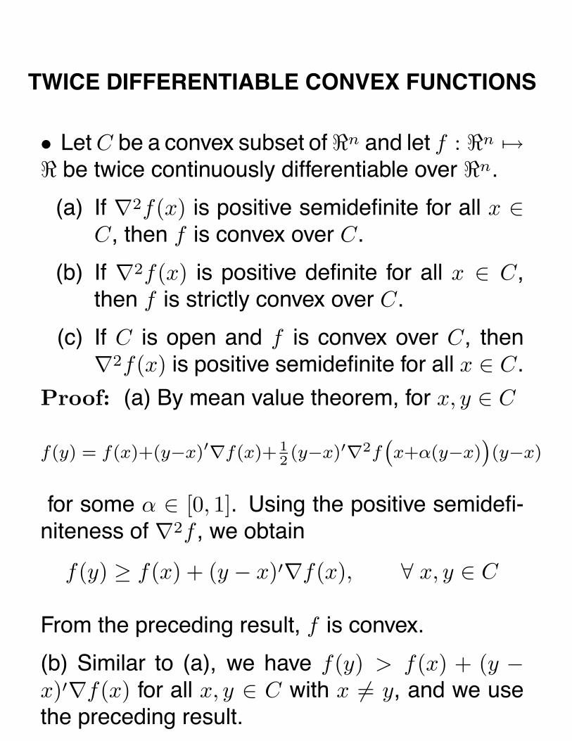
• Let C be a convex subset of �n and let f : �n �→� be twice continuously differentiable over �n.
(a) If ∇2f(x) is positive semidefinite for all x ∈C, then f is convex over C.
(b) If ∇2f(x) is positive definite for all x ∈ C,then f is strictly convex over C.
(c) If C is open and f is convex over C, then∇2f(x) is positive semidefinite for all x ∈ C.
Proof: (a) By mean value theorem, for x, y ∈ C
f(y) = f(x)+(y−x)′∇f(x)+ 12(y−x)′∇2f
(x+α(y−x)
)(y−x)
for some α ∈ [0, 1]. Using the positive semidefi-niteness of ∇2f , we obtain
f(y) ≥ f(x) + (y − x)′∇f(x), ∀ x, y ∈ C
From the preceding result, f is convex.
(b) Similar to (a), we have f(y) > f(x) + (y −x)′∇f(x) for all x, y ∈ C with x �= y, and we usethe preceding result.

CONVEX AND AFFINE HULLS
• Given a set X ⊂ �n:
• A convex combination of elements of X is avector of the form
∑mi=1 αixi, where xi ∈ X, αi ≥
0, and∑m
i=1 αi = 1.
• The convex hull of X, denoted conv(X), is theintersection of all convex sets containing X (alsothe set of all convex combinations from X).
• The affine hull of X, denoted aff(X), is the in-tersection of all affine sets containing X (an affineset is a set of the form x + S, where S is a sub-space). Note that aff(X) is itself an affine set.
• A nonnegative combination of elements of X isa vector of the form
∑mi=1 αixi, where xi ∈ X and
αi ≥ 0 for all i.
• The cone generated by X, denoted cone(X), isthe set of all nonnegative combinations from X:
− It is a convex cone containing the origin.
− It need not be closed.
− If X is a finite set, cone(X) is closed (non-trivial to show!)

CARATHEODORY’S THEOREM
X
cone(X)
x1
x2
0
x1
x2
x4
x3
conv(X)
x
(a) (b)
x
• Let X be a nonempty subset of �n.
(a) Every x �= 0 in cone(X) can be representedas a positive combination of vectors x1, . . . , xm
from X that are linearly independent.
(b) Every x /∈ X that belongs to conv(X) canbe represented as a convex combination ofvectors x1, . . . , xm from X such that x2 −x1, . . . , xm − x1 are linearly independent.

PROOF OF CARATHEODORY’S THEOREM
(a) Let x be a nonzero vector in cone(X), and letm be the smallest integer such that x has theform
∑mi=1 αixi, where αi > 0 and xi ∈ X for
all i = 1, . . . , m. If the vectors xi were linearlydependent, there would exist λ1, . . . , λm, with
m∑i=1
λixi = 0
and at least one of the λi is positive. Considerm∑
i=1
(αi − γλi)xi,
where γ is the largest γ such that αi − γλi ≥ 0 forall i. This combination provides a representationof x as a positive combination of fewer than m vec-tors of X – a contradiction. Therefore, x1, . . . , xm,are linearly independent.
(b) Apply part (a) to the subset of �n+1
Y ={(x, 1) | x ∈ X
}

AN APPLICATION OF CARATHEODORY
• The convex hull of a compact set is compact.
Proof: Let X be compact. We take a sequencein conv(X) and show that it has a convergent sub-sequence whose limit is in conv(X).
By Caratheodory, a sequence in conv(X)can be expressed as
{∑n+1i=1 αk
i xki
}, where for all
k and i, αki ≥ 0, xk
i ∈ X, and∑n+1
i=1 αki = 1. Since
the sequence
{(αk
1 , . . . , αkn+1, x
k1 , . . . , xk
n+1)}
is bounded, it has a limit point
{(α1, . . . , αn+1, x1, . . . , xn+1)
},
which must satisfy∑n+1
i=1 αi = 1, and αi ≥ 0,xi ∈ X for all i. Thus, the vector
∑n+1i=1 αixi,
which belongs to conv(X), is a limit point of the
sequence{∑n+1
i=1 αki xk
i
}, showing that conv(X)
is compact. Q.E.D.

RELATIVE INTERIOR
• x is a relative interior point of C, if x is aninterior point of C relative to aff(C).
• ri(C) denotes the relative interior of C, i.e., theset of all relative interior points of C.
• Line Segment Principle: If C is a convex set,x ∈ ri(C) and x ∈ cl(C), then all points on the linesegment connecting x and x, except possibly x,belong to ri(C).
S
Sα
x
ε
α εx
xα = αx + (1 - α)x
C

ADDITIONAL MAJOR RESULTS
• Let C be a nonempty convex set.
(a) ri(C) is a nonempty convex set, and has thesame affine hull as C.
(b) x ∈ ri(C) if and only if every line segmentin C having x as one endpoint can be pro-longed beyond x without leaving C.
X
z1
0
C
z2
Proof: (a) Assume that 0 ∈ C. We choose m lin-early independent vectors z1, . . . , zm ∈ C, wherem is the dimension of aff(C), and we let
X =
{m∑
i=1
αizi
∣∣∣ m∑i=1
αi < 1, αi > 0, i = 1, . . . , m
}
(b) => is clear by the def. of rel. interior. Reverse:take any x ∈ ri(C); use Line Segment Principle.

OPTIMIZATION APPLICATION
• A concave function f : �n �→ � that attains itsminimum over a convex set X at an x∗ ∈ ri(X)must be constant over X.
aff(X)
x*x
x
X
Proof: (By contradiction.) Let x ∈ X be suchthat f(x) > f(x∗). Prolong beyond x∗ the linesegment x-to-x∗ to a point x ∈ X. By concavityof f , we have for some α ∈ (0, 1)
f(x∗) ≥ αf(x) + (1 − α)f(x),
and since f(x) > f(x∗), we must have f(x∗) >f(x) - a contradiction. Q.E.D.

LECTURE 4
LECTURE OUTLINE
• Review of relative interior
• Algebra of relative interiors and closures
• Continuity of convex functions
• Recession cones***********************************
• Recall: x is a relative interior point of C, if x isan interior point of C relative to aff(C)
• Three important properties of ri(C) of a convexset C:
− ri(C) is nonempty
− Line Segment Principle: If x ∈ ri(C) andx ∈ cl(C), then all points on the line seg-ment connecting x and x, except possibly x,belong to ri(C)
− Prolongation Principle: If x ∈ ri(C) and x ∈C, the line segment connecting x and x canbe prolonged beyond x without leaving C

A SUMMARY OF FACTS
• The closure of a convex set is equal to the clo-sure of its relative interior.
• The relative interior of a convex set is equal tothe relative interior of its closure.
• Relative interior and closure commute with Carte-sian product and inverse image under a lineartransformation.
• Relative interior commutes with image under alinear transformation and vector sum, but closuredoes not.
• Neither closure nor relative interior commutewith set intersection.

CLOSURE VS RELATIVE INTERIOR
• Let C be a nonempty convex set. Then ri(C)and cl(C) are “not too different for each other.”
• Proposition:
(a) We have cl(C) = cl(ri(C)
).
(b) We have ri(C) = ri(cl(C)
).
(c) Let C be another nonempty convex set. Thenthe following three conditions are equivalent:
(i) C and C have the same rel. interior.
(ii) C and C have the same closure.
(iii) ri(C) ⊂ C ⊂ cl(C).
Proof: (a) Since ri(C) ⊂ C, we have cl(ri(C)
)⊂
cl(C). Conversely, let x ∈ cl(C). Let x ∈ ri(C).By the Line Segment Principle, we have αx+(1−α)x ∈ ri(C) for all α ∈ (0, 1]. Thus, x is the limit ofa sequence that lies in ri(C), so x ∈ cl
(ri(C)
).
x
xC

LINEAR TRANSFORMATIONS
• Let C be a nonempty convex subset of �n andlet A be an m × n matrix.
(a) We have A · ri(C) = ri(A · C).
(b) We have A · cl(C) ⊂ cl(A ·C). Furthermore,if C is bounded, then A · cl(C) = cl(A · C).
Proof: (a) Intuition: Spheres within C are mappedonto spheres within A·C (relative to the affine hull).
(b) We have A · cl(C) ⊂ cl(A · C), since if a se-quence {xk} ⊂ C converges to some x ∈ cl(C)then the sequence {Axk}, which belongs to A ·C,converges to Ax, implying that Ax ∈ cl(A · C).
To show the converse, assuming that C isbounded, choose any z ∈ cl(A · C). Then, thereexists a sequence {xk} ⊂ C such that Axk → z.Since C is bounded, {xk} has a subsequence thatconverges to some x ∈ cl(C), and we must haveAx = z. It follows that z ∈ A · cl(C). Q.E.D.
Note that in general, we may have
A · int(C) �= int(A · C), A · cl(C) �= cl(A · C)

INTERSECTIONS AND VECTOR SUMS
• Let C1 and C2 be nonempty convex sets.
(a) We have
ri(C1 + C2) = ri(C1) + ri(C2),
cl(C1) + cl(C2) ⊂ cl(C1 + C2)
If one of C1 and C2 is bounded, then
cl(C1) + cl(C2) = cl(C1 + C2)
(b) If ri(C1) ∩ ri(C2) �= Ø, then
ri(C1 ∩ C2) = ri(C1) ∩ ri(C2),
cl(C1 ∩ C2) = cl(C1) ∩ cl(C2)
Proof of (a): C1 + C2 is the result of the lineartransformation (x1, x2) �→ x1 + x2.
• Counterexample for (b):
C1 = {x | x ≤ 0}, C2 = {x | x ≥ 0}

CONTINUITY OF CONVEX FUNCTIONS
• If f : �n �→ � is convex, then it is continuous.
e1
xk
xk+1
0
yke3 e2
e4 zk
Proof: We will show that f is continuous at 0. Byconvexity, f is bounded within the unit cube by themaximum value of f over the corners of the cube.
Consider sequence xk → 0 and the sequencesyk = xk/‖xk‖∞, zk = −xk/‖xk‖∞. Then
f(xk) ≤(1 − ‖xk‖∞
)f(0) + ‖xk‖∞f(yk)
f(0) ≤ ‖xk‖∞‖xk‖∞ + 1
f(zk) +1
‖xk‖∞ + 1f(xk)
Since ‖xk‖∞ → 0, f(xk) → f(0). Q.E.D.
• Extension to continuity over ri(dom(f)).

RECESSION CONE OF A CONVEX SET
• Given a nonempty convex set C, a vector y isa direction of recession if starting at any x in Cand going indefinitely along y, we never cross therelative boundary of C to points outside C:
x + αy ∈ C, ∀ x ∈ C, ∀ α ≥ 0
0
x + αy
x
Convex Set C
Recession Cone RC
y
• Recession cone of C (denoted by RC): The setof all directions of recession.
• RC is a cone containing the origin.

RECESSION CONE THEOREM
• Let C be a nonempty closed convex set.
(a) The recession cone RC is a closed convexcone.
(b) A vector y belongs to RC if and only if thereexists a vector x ∈ C such that x + αy ∈ Cfor all α ≥ 0.
(c) RC contains a nonzero direction if and onlyif C is unbounded.
(d) The recession cones of C and ri(C) are equal.
(e) If D is another closed convex set such thatC ∩ D �= Ø, we have
RC∩D = RC ∩ RD
More generally, for any collection of closedconvex sets Ci, i ∈ I, where I is an arbitraryindex set and ∩i∈ICi is nonempty, we have
R∩i∈ICi = ∩i∈IRCi

PROOF OF PART (B)
x
z1 = x + y
z2
z3
x_
x + y_
x + y1_ x + y2
_ x + y3_
C
• Let y �= 0 be such that there exists a vectorx ∈ C with x + αy ∈ C for all α ≥ 0. We fix x ∈ Cand α > 0, and we show that x + αy ∈ C. Byscaling y, it is enough to show that x + y ∈ C.
Let zk = x + ky for k = 1, 2, . . ., and yk =(zk − x)‖y‖/‖zk − x‖. We have
yk
‖y‖=
‖zk − x‖‖zk − x‖
y
‖y‖+
x − x
‖zk − x‖,
‖zk − x‖‖zk − x‖
→ 1,x − x
‖zk − x‖→ 0,
so yk → y and x + yk → x + y. Use the convexityand closedness of C to conclude that x + y ∈ C.

LINEALITY SPACE
• The lineality space of a convex set C, denoted byLC , is the subspace of vectors y such that y ∈ RC
and −y ∈ RC :
LC = RC ∩ (−RC)
• Decomposition of a Convex Set: Let C be anonempty convex subset of �n. Then,
C = LC + (C ∩ L⊥C).
Also, if LC = RC , the component C ∩ L⊥C is com-
pact (this will be shown later).
C
0
S
S
C∩S
x
y
z

LECTURE 5
LECTURE OUTLINE
• Directions of recession of convex functions
• Existence of optimal solutions - Weierstrass’theorem
• Intersection of nested sequences of closed sets
• Asymptotic directions
−−−−−−−−−−−−−−−−−−−−−−−−• For a closed convex set C, recall that y is adirection of recession if x + αy ∈ C, for all x ∈ Cand α ≥ 0.
0
x + αy
x
Convex Set C
Recession Cone RC
y
• Recession cone theorem: If this property istrue for one x ∈ C, it is true for all x ∈ C; also Cis compact iff RC = {0}.

DIRECTIONS OF RECESSION OF A FUNCTION
• Some basic geometric observations:
− The “horizontal directions” in the recessioncone of the epigraph of a convex function fare directions along which the level sets areunbounded.
− Along these directions the level sets{x |
f(x) ≤ γ}
are unbounded and f is mono-tonically nondecreasing.
• These are the directions of recession of f .
γ
epi(f)
Level Set Vγ = {x | f(x) ≤ γ}
“Slice” {(x,γ) | f(x) ≤ γ}
RecessionCone of f
0

RECESSION CONE OF LEVEL SETS
• Proposition: Let f : �n �→ (−∞,∞] be a closedproper convex function and consider the level setsVγ =
{x | f(x) ≤ γ
}, where γ is a scalar. Then:
(a) All the nonempty level sets Vγ have the samerecession cone, given by
RVγ ={y | (y, 0) ∈ Repi(f)
}(b) If one nonempty level set Vγ is compact, then
all nonempty level sets are compact.
Proof: For all γ for which Vγ is nonempty,
{(x, γ) | x ∈ Vγ
}= epi(f) ∩
{(x, γ) | x ∈ �n
}The recession cone of the set on the left is
{(y, 0) |
y ∈ RVγ
}. The recession cone of the set on the
right is the intersection of Repi(f) and the reces-sion cone of
{(x, γ) | x ∈ �n
}. Thus we have
{(y, 0) | y ∈ RVγ
}=
{(y, 0) | (y, 0) ∈ Repi(f)
},
from which the result follows.

RECESSION CONE OF A CONVEX FUNCTION
• For a closed proper convex function f : �n �→(−∞,∞], the (common) recession cone of thenonempty level sets Vγ =
{x | f(x) ≤ γ
}, γ ∈ �,
is the recession cone of f , and is denoted by Rf .
0
Level Sets of ConvexFunction f
Recession Cone Rf
• Terminology:
− y ∈ Rf : a direction of recession of f .
− Lf = Rf ∩ (−Rf ): the lineality space of f .
− y ∈ Lf : a direction of constancy of f .
− Function rf : �n �→ (−∞,∞] whose epi-graph is Repi(f): the recession function of f .
• Note: rf (y) is the “asymptotic slope” of f in thedirection y. In fact, rf (y) = limα→∞ ∇f(x+αy)′yif f is differentiable. Also, y ∈ Rf iff rf (y) ≤ 0.

DESCENT BEHAVIOR OF A CONVEX FUNCTION
f(x + αy)
α
f(x)
(a)
f(x + αy)
α
f(x)
(b)
f(x + αy)
α
f(x)
(c)
f(x + αy)
α
f(x)
(d)
f(x + αy)
α
f(x)
(e)
f(x + αy)
α
f(x)
(f)
• y is a direction of recession in (a)-(d).
• This behavior is independent of the startingpoint x, as long as x ∈ dom(f).

EXISTENCE OF SOLUTIONS - BOUNDED CASE
Proposition: The set of minima of a closed properconvex function f : �n �→ (−∞,∞] is nonemptyand compact if and only if f has no nonzero direc-tion of recession.
Proof: Let X∗ be the set of minima, let f∗ =infx∈�n f(x), and let {γk} be a scalar sequencesuch that γk ↓ f∗. Note that
X∗ = ∩∞k=0
(X ∩
{x | f(x) ≤ γk
})If f has no nonzero direction of recession,
the sets X ∩{x | f(x) ≤ γk
}are nonempty, com-
pact, and nested, so X∗ is nonempty and com-pact.
Conversely, we have
X∗ ={x | f(x) ≤ f∗
},
so if X∗ is nonempty and compact, all the levelsets of f are compact and f has no nonzero di-rection of recession. Q.E.D.

SPECIALIZATION/GENERALIZATION OF THE IDEA
• Important special case: Minimize a real-valued function f : �n �→ � over a nonemptyset X. Apply the preceding proposition to the ex-tended real-valued function
f(x) ={
f(x) if x ∈ X,∞ otherwise.
• The set intersection/compactness argument gen-eralizes to nonconvex.Weierstrass’ Theorem: The set of minima of fover X is nonempty and compact if X is closed,f is lower semicontinuous over X, and one of thefollowing conditions holds:
(1) X is bounded.
(2) Some set{x ∈ X | f(x) ≤ γ
}is nonempty
and bounded.
(3) f is coercive, i.e., for every sequence {xk} ⊂X s. t. ‖xk‖ → ∞, we have limk→∞ f(xk) =∞.
Proof: In all cases the level sets of f are com-pact. Q.E.D.

THE ROLE OF CLOSED SET INTERSECTIONS
• A fundamental question: Given a sequenceof nonempty closed sets {Sk} in �n with Sk+1 ⊂Sk for all k, when is ∩∞
k=0Sk nonempty?
• Set intersection theorems are significant in atleast three major contexts, which we will discussin what follows:
1. Does a function f : �n �→ (−∞,∞] attain aminimum over a set X? This is true iff the in-tersection of the nonempty level sets
{x ∈ X |
f(x) ≤ γk
}is nonempty.
2. If C is closed and A is a matrix, is A C closed?Special case:
− If C1 and C2 are closed, is C1 + C2 closed?
3. If F (x, z) is closed, is f(x) = infz F (x, z) closed?(Critical question in duality theory.) Can be ad-dressed by using the relation
P(epi(F )
)⊂ epi(f) ⊂ cl
(P
(epi(F )
))
where P (·) is projection on the space of (x, w).

ASYMPTOTIC DIRECTIONS
• Given a sequence of nonempty nested closedsets {Sk}, we say that a vector d �= 0 is an asymp-totic direction of {Sk} if there exists {xk} s. t.
xk ∈ Sk, xk �= 0, k = 0, 1, . . .
‖xk‖ → ∞,xk
‖xk‖→ d
‖d‖
• A sequence {xk} associated with an asymp-totic direction d as above is called an asymptoticsequence corresponding to d.
x0
x1
x2
x3
x4
x5
x6
S0
S2
S1
0
d
S3
Asymptotic Direction
Asymptotic Sequence

CONNECTION WITH RECESSION CONES
• We say that d is an asymptotic direction of anonempty closed set S if it is an asymptotic direc-tion of the sequence {Sk}, where Sk = S for allk.
• Notation: The set of asymptotic directions ofS is denoted AS .
• Important facts:− The set of asymptotic directions of a closed
set sequence {Sk} is
∩∞k=0ASk
− For a closed convex set S
AS = RS \ {0}
− The set of asymptotic directions of a closedconvex set sequence {Sk} is
∩∞k=0RSk \ {0}

LECTURE 6
LECTURE OUTLINE
• Asymptotic directions that are retractive
• Nonemptiness of closed set intersections
• Frank-Wolfe Theorem
• Horizon directions
• Existence of optimal solutions
• Preservation of closure under linear transfor-mation and partial minimization
−−−−−−−−−−−−−−−−−−Asymptotic directions of a closed set sequence
x0
x1
x2
x3
x4
x5
x6
S0
S2
S1
0
d
S3
Asymptotic Direction
Asymptotic Sequence

RETRACTIVE ASYMPTOTIC DIRECTIONS
• Consider a nested closed set sequence {Sk}.
• An asymptotic direction d is called retractive iffor every asymptotic sequence {xk} there existsan index k such that
xk − d ∈ Sk, ∀ k ≥ k.
• {Sk} is called retractive if all its asymptotic di-rections are retractive.
• These definitions specialize to closed convexsets S by taking Sk ≡ S.
x0
x1
x2
S0
S2
S1
0
d
(a)
S0
S1
S2
x0
x1
x20
d
(b)

SET INTERSECTION THEOREM
• If {Sk} is retractive, then ∩∞k=0 Sk is nonempty.
• Key proof ideas:
(a) The intersection ∩∞k=0 Sk is empty iff there is
an unbounded sequence {xk} consisting ofminimum norm vectors from the Sk.
(b) An asymptotic sequence {xk} consisting ofminimum norm vectors from the Sk cannotbe retractive, because such a sequence even-tually gets closer to 0 when shifted oppositeto the asymptotic direction.
x0
x1
x2x3
x4 x5
0d
Asymptotic Direction
Asymptotic Sequence

RECOGNIZING RETRACTIVE SETS
• Unions, intersections, and Cartesian produstsof retractive sets are retractive.
• The complement of an open convex set is re-tractive.
C: Open, convexS: Closed
x0
xk+1xk
x1d
d
d
d
• Closed halfspaces are retractive.
• Polyhedral sets are retractive.
• Sets of the form{x | fj(x) ≥ 0, j = 1, . . . , r
},
where fj : �n �→ � is convex, are retractive.
• Vector sum of a compact set and a retractiveset is retractive.
• Nonpolyhedral cones are not retractive, levelsets of quadratic functions are not retractive.

LINEAR AND QUADRATIC PROGRAMMING
• Frank-Wolfe Theorem: Let
f(x) = x′Qx+c′x, X = {x | a′jx+bj ≤ 0, j = 1, . . . , r},
where Q is symmetric (not necessarily positivesemidefinite). If the minimal value of f over Xis finite, there exists a minimum of f of over X.
• Proof (outline): Choose {γk} s.t. γk ↓ f∗,where f∗ is the optimal value, and let
Sk = {x ∈ X | x′Qx + c′x ≤ γk}
The set of optimal solutions is ∩∞k=0 Sk, so it will
suffice to show that for each asymptotic direc-tion of {Sk}, each corresponding asymptotic se-quence is retractive.
Choose an asymptotic direction d and a cor-responding asymptotic sequence. Note that Xis retractive, so for k sufficiently large, we havexk − d ∈ X.

PROOF OUTLINE – CONTINUED
• We use the relation x′kQxk + c′xk ≤ γk to show
that
d′Qd ≤ 0, a′jd ≤ 0, j = 1, . . . , r
• Then show, using the finiteness of f∗ [whichimplies f(x + αd) ≥ f∗ for all x ∈ X], that
(c + 2Qx)′d ≥ 0, ∀ x ∈ X
• Thus,
f(xk−d) = (xk − d)′Q(xk − d) + c′(xk − d)= xk
′Qxk + c′xk − (c + 2Qxk)′d + d′Qd
≤ xk′Qxk + c′xk
≤ γk,
so xk − d ∈ Sk. Q.E.D.

INTERSECTION THEOREM FOR CONVEX SETS
Let {Ck} be a nested sequence of nonemptyclosed convex sets. Denote
R = ∩∞k=0RCk , L = ∩∞
k=0LCk .
(a) If R = L, then {Ck} is retractive, and∩∞k=0 Ck
is nonempty. Furthermore, we have
∩∞k=0Ck = L + C,
where C is some nonempty and compactset.
(b) Let X be a retractive closed set. Assumethat all the sets Sk = X ∩ Ck are nonempty,and that
AX ∩ R ⊂ L.
Then, {Sk} is retractive, and∩∞k=0 Sk is nonempty.

CRITICAL ASYMPTOTES
• Retractiveness works well for sets with a polyhe-dral structure, but not for sets specified by convexquadratic inequalities.
• Key question: Given nested sequences {S1k}
and {S2k} each with nonempty intersection by it-
self, and with
S1k ∩ S2
k �= Ø, k = 0, 1, . . . ,
what causes the intersection sequence {S1k ∩S2
k}to have an empty intersection?
• The trouble lies with the existence of some “crit-ical asymptotes.”
S2
Sk1
d: “Critical Asymptote”

HORIZON DIRECTIONS
• Consider {Sk}with∩∞k=0 Sk �= Ø. An asymptotic
direction d of {Sk} is:
(a) A local horizon direction if, for every x ∈∩∞
k=0 Sk, there exists a scalar α ≥ 0 suchthat x + αd ∈ ∩∞
k=0 Sk for all α ≥ α.
(b) A global horizon direction if for every x ∈ �n
there exists a scalar α ≥ 0 such that x+αd ∈∩∞
k=0 Sk for all α ≥ α.
• Example: (2-D Convex Quadratic Set Se-quences)
Sk = {(x1,x2) | x1 - x2 ≤ 1/k}2
x1
x2
0Sk
Sk+1
Sk = {(x1,x2) | x1 ≤ 1/k}2
x1
x2
0
Sk
Sk+1
Directions (0,γ), γ ≠ 0,are local horizon directions
that are retractive
Directions (0,γ), γ > 0,are global horizon directions

GENERAL CONVEX QUADRATIC SETS
• Let Sk ={x | x′Qx + a′x + b ≤ γk
}, where
γk ↓ 0. Then, if all the sets Sk are nonempty,∩∞
k=0Sk �= Ø.
• Asymptotic directions: d �= 0 such that Qd = 0and a′d ≤ 0. There are two possibilities:
(a) Qd = 0 and a′d < 0, in which case d is aglobal horizon direction.
(b) Qd = 0 and a′d = 0, in which case d isa direction of constancy of f , and it followsthat d is a retractive local horizon direction.
• Drawing some 2-dimensional pictures and us-ing the structure of asymptotic directions demon-strated above, we conjecture that there are no“critical asymptotes” for set sequences of the form{S1
k ∩ S2k} when S1
k and S2k are convex quadratic
sets.
• This motivates a general definition of noncriticalasymptotic direction.

CRITICAL DIRECTIONS
• Given a nested closed set sequence {Sk} withnonempty intersection, we say that an asymptoticdirection d of {Sk} is noncritical if d is either aglobal horizon direction of {Sk}, or a retractivelocal horizon direction of {Sk}.
• Proposition: Let Sk = S1k∩S2
k∩· · ·∩Srk, where
{Sjk} are nested sequence such that
Sk �= Ø, ∀ k, ∩∞k=0 Sj
k �= Ø, ∀ j.
Assume that all the asymptotic directions of all{Sj
k} are noncritical. Then ∩∞k=0 Sk �= Ø.
• Special case: (Convex Quadratic Inequal-ities) Let
Sk ={x | x′Qjx + a′
jx + bj ≤ γjk, j = 1, . . . , r
}where {γj
k} are scalar sequences with γjk ↓ 0. As-
sume that Sk �= Ø is nonempty for all k. Then,∩∞
k=0 Sk �= Ø.

APPLICATION TO QUADRATIC MINIMIZATION
• Letf(x) = x′Qx + c′x,
X = {x | x′Rjx + a′jx + bj ≤ 0, j = 1, . . . , r},
where Q and Rj are positive semidefinite matri-ces. If the minimal value of f over X is finite, thereexists a minimum of f of over X.
Proof: Let f∗ be the minimal value, and let γk ↓f∗. The set of optimal solutions is
X∗ = ∩∞k=0
(X ∩ {x | x′Qx + c′x ≤ γk}
).
All the set sequences involved in the intersectionare convex quadratic and hence have no criticaldirections. By the preceding proposition, X∗ isnonenpty. Q.E.D.

CLOSURE UNDER LINEAR TRANSFORMATIONS
• Let C be a nonempty closed convex, and let Abe a matrix with nullspace N(A).
(a) A C is closed if RC ∩ N(A) ⊂ LC .
(b) A(X ∩ C) is closed if X is a polyhedral setand
RX ∩ RC ∩ N(A) ⊂ LC ,
(c) AC is closed if C = {x | fj(x) ≤ 0, j =1, . . . , r}with fj : convex quadratic functions.
Proof: (Outline) Let {yk} ⊂ A C with yk → y.We prove ∩∞
k=0Sk �= Ø, where Sk = C ∩ Nk, and
Nk = {x | Ax ∈ Wk}, Wk ={z | ‖z−y‖ ≤ ‖yk−y‖
}
C
AC
y
x
ykyk+1
Wk
Sk
Nk

LECTURE 7
LECTURE OUTLINE
• Existence of optimal solutions
• Preservation of closure under partial minimiza-tion
• Hyperplane separation
• Nonvertical hyperplanes
• Min common and max crossing problems−−−−−−−−−−−−−−−−−−−−−−−−−−−−• We have talked so far about set intersection the-orems that use two types of asymptotic directions:
− Retractive directions (mostly for polyhedral-type sets)
− Horizon directions (for special types of sets- e.g., quadratic)
• We now apply these theorems to issues ofexistence of optimal solutions, and preservationof closedness under linear transformation, vectorsum, and partial minimization.

PROJECTION THEOREM
• Let C be a nonempty closed convex set in �n.
(a) For every x ∈ �n, there exists a unique vec-tor PC(x) that minimizes ‖z − x‖ over allz ∈ C (called the projection of x on C).
(b) For every x ∈ �n, a vector z ∈ C is equal toPC(x) if and only if
(y − z)′(x − z) ≤ 0, ∀ y ∈ C
In the case where C is an affine set, theabove condition is equivalent to
x − z ∈ S⊥,
where S is the subspace that is parallel toC.
(c) The function f : �n �→ C defined by f(x) =PC(x) is continuous and nonexpansive, i.e.,
∥∥PC(x)−PC(y)∥∥ ≤ ‖x−y‖, ∀ x, y ∈ �n

EXISTENCE OF OPTIMAL SOLUTIONS
• Let X and f : �n �→ (−∞,∞] be closed convexand such that X∩dom(f) �= Ø. The set of minimaof f over X is nonempty under any one of thefollowing three conditions:
(1) RX ∩ Rf = LX ∩ Lf .
(2) RX ∩ Rf ⊂ Lf , and X is polyhedral.
(3) f∗ > −∞, and f and X are specified byconvex quadratic functions:
f(x) = x′Qx + c′x,
X ={x | x′Qjx+a′
jx+bj ≤ 0, j = 1, . . . , r}.
Proof: Follows by writing
Set of Minima = ∩ (Nonempty Level Sets)
and by applying the corresponding set intersec-tion theorems. Q.E.D.

EXISTENCE OF OPTIMAL SOLUTIONS: EXAMPLE
(a)(b)
0 x1
x2
Level Sets of Convex Function f
Constancy Space Lf
X
0 x1
x2
Level Sets of Convex Function f
Constancy Space Lf
X
• Here f(x1, x2) = ex1 .
• In (a), X is polyhedral, and the minimum isattained.
• In (b),
X ={(x1, x2) | x2
1 ≤ x2
}We have RX ∩ Rf ⊂ Lf , but the minimum is notattained (X is not polyhedral).

PARTIAL MINIMIZATION THEOREM
• Let F : �n+m �→ (−∞,∞] be a closed properconvex function, and consider f(x) = infz∈�m F (x, z).
• Each of the major set intersection theoremsyields a closedness result. The simplest case isthe following:
• Preservation of Closedness Under Com-pactness: If there exist x ∈ �n, γ ∈ � such thatthe set {
z | F (x, z) ≤ γ}
is nonempty and compact, then f is convex, closed,and proper. Also, for each x ∈ dom(f), the set ofminima of F (x, ·) is nonempty and compact.
Proof: (Outline) By the hypothesis, there is nononzero y such that (0, y, 0) ∈ Repi(F ). Also, allthe nonempty level sets
{z | F (x, z) ≤ γ}, x ∈ �n, γ ∈ �,
have the same recession cone, which by hypoth-esis, is equal to {0}.

HYPERPLANES
Positive Halfspace{x | a'x ≥ b}
a
Negative Halfspace{x | a'x ≤ b}
x
Hyperplane{x | a'x = b} = {x | a'x = a'x}
_
_
• A hyperplane is a set of the form {x | a′x = b},where a is nonzero vector in �n and b is a scalar.
• We say that two sets C1 and C2 are separatedby a hyperplane H = {x | a′x = b} if each lies in adifferent closed halfspace associated with H, i.e.,
either a′x1 ≤ b ≤ a′x2, ∀x1 ∈ C1, ∀x2 ∈ C2,
or a′x2 ≤ b ≤ a′x1, ∀ x1 ∈ C1, ∀ x2 ∈ C2
• If x belongs to the closure of a set C, a hyper-plane that separates C and the singleton set {x}is said be supporting C at x.

VISUALIZATION
• Separating and supporting hyperplanes:
a C2
C1
(a)
a
C
(b)
x
• A separating {x | a′x = b} that is disjoint fromC1 and C2 is called strictly separating:
a′x1 < b < a′x2, ∀ x1 ∈ C1, ∀ x2 ∈ C2
(b)(a)
C2 = {(ξ1,ξ2) | ξ1 > 0, ξ2 >0, ξ1ξ2 ≥ 1}
C1 = {(ξ1,ξ2) | ξ1 ≤ 0}
a
C1
C2x2
x1
x

SUPPORTING HYPERPLANE THEOREM
• Let C be convex and let x be a vector that isnot an interior point of C. Then, there exists ahyperplane that passes through x and contains Cin one of its closed halfspaces.
x3x2
x1
x0
a2
a1
a0
C
x2 x1
x0
x
x3
Proof: Take a sequence {xk} that does not be-long to cl(C) and converges to x. Let xk be theprojection of xk on cl(C). We have for all x ∈ cl(C)
a′kx ≥ a′
kxk, ∀ x ∈ cl(C), ∀ k = 0, 1, . . . ,
where ak = (xk − xk)/‖xk − xk‖. Le a be a limitpoint of {ak}, and take limit as k → ∞. Q.E.D.

SEPARATING HYPERPLANE THEOREM
• Let C1 and C2 be two nonempty convex subsetsof �n. If C1 and C2 are disjoint, there exists ahyperplane that separates them, i.e., there existsa vector a �= 0 such that
a′x1 ≤ a′x2, ∀ x1 ∈ C1, ∀ x2 ∈ C2.
Proof: Consider the convex set
C1 − C2 = {x2 − x1 | x1 ∈ C1, x2 ∈ C2}
Since C1 and C2 are disjoint, the origin does notbelong to C1 − C2, so by the Supporting Hyper-plane Theorem, there exists a vector a �= 0 suchthat
0 ≤ a′x, ∀ x ∈ C1 − C2,
which is equivalent to the desired relation. Q.E.D.

STRICT SEPARATION THEOREM
• Strict Separation Theorem: Let C1 and C2
be two disjoint nonempty convex sets. If C1 isclosed, and C2 is compact, there exists a hyper-plane that strictly separates them.
(b)(a)
C2 = {(ξ1,ξ2) | ξ1 > 0, ξ2 >0, ξ1ξ2 ≥ 1}
C1 = {(ξ1,ξ2) | ξ1 ≤ 0}
a
C1
C2x2
x1
x
Proof: (Outline) Consider the set C1−C2. SinceC1 is closed and C2 is compact, C1−C2 is closed.Since C1 ∩ C2 = Ø, 0 /∈ C1 − C2. Let x1 − x2
be the projection of 0 onto C1 − C2. The strictlyseparating hyperplane is constructed as in (b).
• Note: Any conditions that guarantee closed-ness of C1 − C2 guarantee existence of a strictlyseparating hyperplane. However, there may exista strictly separating hyperplane without C1 − C2
being closed.

ADDITIONAL THEOREMS
• Fundamental Characterization: The clo-sure of the convex hull of a set C ⊂ �n is theintersection of the closed halfspaces that containC.
• We say that a hyperplane properly separates C1
and C2 if it separates C1 and C2 and does not fullycontain both C1 and C2.
a
C2
C1Separatinghyperplane
(b)(a)
a
C2
C1
Separatinghyperplane
• Proper Separation Theorem: Let C1 and C2
be two nonempty convex subsets of�n. There ex-ists a hyperplane that properly separates C1 andC2 if and only if
ri(C1) ∩ ri(C2) = Ø

MIN COMMON / MAX CROSSING PROBLEMS
• We introduce a pair of fundamental problems:
• Let M be a nonempty subset of �n+1
(a) Min Common Point Problem: Consider allvectors that are common to M and the (n +1)st axis. Find one whose (n + 1)st compo-nent is minimum.
(b) Max Crossing Point Problem: Consider “non-vertical” hyperplanes that contain M in their“upper” closed halfspace. Find one whosecrossing point of the (n + 1)st axis is maxi-mum.
0
Min Common Point w*
Max Crossing Point q*
M
w
0
M
Max Crossing Point q*
Min Common Point w*w
uu
• We first need to study “nonvertical” hyperplanes.

NONVERTICAL HYPERPLANES
• A hyperplane in �n+1 with normal (µ, β) is non-vertical if β �= 0.
• It intersects the (n+1)st axis at ξ = (µ/β)′u+w,where (u, w) is any vector on the hyperplane.
(µ,β)
w
uNonverticalHyperplane
(µ,0)
VerticalHyperplane
(u,w)__
(µ/β)' u + w__
0
• A nonvertical hyperplane that contains the epi-graph of a function in its “upper” halfspace, pro-vides lower bounds to the function values.
• The epigraph of a proper convex function doesnot contain a vertical line, so it appears plausi-ble that it is contained in the “upper” halfspace ofsome nonvertical hyperplane.

NONVERTICAL HYPERPLANE THEOREM
• Let C be a nonempty convex subset of �n+1
that contains no vertical lines. Then:
(a) C is contained in a closed halfspace of anonvertical hyperplane, i.e., there exist µ ∈�n, β ∈ � with β �= 0, and γ ∈ � such thatµ′u + βw ≥ γ for all (u, w) ∈ C.
(b) If (u, w) /∈ cl(C), there exists a nonverticalhyperplane strictly separating (u, w) and C.
Proof: Note that cl(C) contains no vert. line [sinceC contains no vert. line, ri(C) contains no vert.line, and ri(C) and cl(C) have the same recessioncone]. So we just consider the case: C closed.
(a) C is the intersection of the closed halfspacescontaining C. If all these corresponded to verticalhyperplanes, C would contain a vertical line.
(b) There is a hyperplane strictly separating (u, w)and C. If it is nonvertical, we are done, so assumeit is vertical. “Add” to this vertical hyperplane asmall ε-multiple of a nonvertical hyperplane con-taining C in one of its halfspaces as per (a).

LECTURE 8
LECTURE OUTLINE
• Min Common / Max Crossing problems
• Weak duality
• Strong duality
• Existence of optimal solutions
• Minimax problems
0
Min Common Point w*
Max Crossing Point q*
M
w
0
M
Max Crossing Point q*
Min Common Point w*w
uu

WEAK DUALITY
• Optimal value of the min common problem:
w∗ = inf(0,w)∈M
w
• Math formulation of the max crossing problem:Focus on hyperplanes with normals (µ, 1) whosecrossing point ξ satisfies
ξ ≤ w + µ′u, ∀ (u, w) ∈ M
Max crossing problem is to maximize ξ subject toξ ≤ inf(u,w)∈M{w + µ′u}, µ ∈ �n, or
maximize q(µ)�= inf
(u,w)∈M{w + µ′u}
subject to µ ∈ �n.
• For all (u, w) ∈ M and µ ∈ �n,
q(µ) = inf(u,w)∈M
{w + µ′u} ≤ inf(0,w)∈M
w = w∗,
so maximizing over µ ∈ �n, we obtain q∗ ≤ w∗.
• Note that q is concave and upper-semicontinuous.

STRONG DUALITY
• Question: Under what conditions do we haveq∗ = w∗ and the supremum in the max crossingproblem is attained?
0
(a)
Min Common Point w*
Max Crossing Point q*
M
0
(b)
M
_M
Max Crossing Point q*
Min Common Point w*w w
u
0
(c)
S
_M
MMax Crossing Point q*
Min Common Point w*
w
u
u

DUALITY THEOREMS
• Assume that w∗ < ∞ and that the set
M ={
(u, w) | there exists w with w ≤ w and (u, w) ∈ M}
is convex.
• Min Common/Max Crossing Theorem I : Wehave q∗ = w∗ if and only if for every sequence{(uk, wk)
}⊂ M with uk → 0, there holds w∗ ≤
lim infk→∞ wk.
• Min Common/Max Crossing Theorem II : As-sume in addition that −∞ < w∗ and that the set
D ={u | there exists w ∈ � with (u, w) ∈ M}
contains the origin in its relative interior. Thenq∗ = w∗ and there exists a vector µ ∈ �n such thatq(µ) = q∗. If D contains the origin in its interior, theset of all µ ∈ �n such that q(µ) = q∗ is compact.
• Min Common/Max Crossing Theorem III : In-volves polyhedral assumptions, and will be devel-oped later.

PROOF OF THEOREM I
• Assume that for every sequence{(uk, wk)
}⊂
M with uk → 0, there holds w∗ ≤ lim infk→∞ wk.If w∗ = −∞, then q∗ = −∞, by weak duality, soassume that −∞ < w∗. Steps of the proof:
(1) M does not contain any vertical lines.
(2) (0, w∗ − ε) /∈ cl(M) for any ε > 0.
(3) There exists a nonvertical hyperplane strictlyseparating (0, w∗ − ε) and M . This hyper-plane crosses the (n + 1)st axis at a vector(0, ξ) with w∗− ε ≤ ξ ≤ w∗, so w∗− ε ≤ q∗ ≤w∗. Since ε can be arbitrarily small, it followsthat q∗ = w∗.
Conversely, assume that q∗ = w∗. Let{(uk, wk)
}⊂
M be such that uk → 0. Then,
q(µ) = inf(u,w)∈M
{w+µ′u} ≤ wk+µ′uk, ∀ k, ∀µ ∈ �n
Taking the limit as k → ∞, we obtain q(µ) ≤lim infk→∞ wk, for all µ ∈ �n, implying that
w∗ = q∗ = supµ∈�n
q(µ) ≤ lim infk→∞
wk

PROOF OF THEOREM II
• Note that (0, w∗) is not a relative interior pointof M . Therefore, by the Proper Separation Theo-rem, there exists a hyperplane that passes through(0, w∗), contains M in one of its closed halfspaces,but does not fully contain M , i.e., there exists(µ, β) such that
βw∗ ≤ µ′u + βw, ∀ (u, w) ∈ M,
βw∗ < sup(u,w)∈M
{µ′u + βw}
Since for any (u, w) ∈ M , the set M contains thehalfline
{(u, w) | w ≤ w
}, it follows that β ≥ 0. If
β = 0, then 0 ≤ µ′u for all u ∈ D. Since 0 ∈ ri(D)by assumption, we must have µ′u = 0 for all u ∈ Da contradiction. Therefore, β > 0, and we canassume that β = 1. It follows that
w∗ ≤ inf(u,w)∈M
{µ′u + w} = q(µ) ≤ q∗
Since the inequality q∗ ≤ w∗ holds always, wemust have q(µ) = q∗ = w∗.

MINIMAX PROBLEMS
Given φ : X × Z �→ �, where X ⊂ �n, Z ⊂ �m
considerminimize sup
z∈Zφ(x, z)
subject to x ∈ X
andmaximize inf
x∈Xφ(x, z)
subject to z ∈ Z.
• Some important contexts:
− Worst-case design. Special case: Minimizeover x ∈ X
max{f1(x), . . . , fm(x)
}− Duality theory and zero sum game theory
(see the next two slides)
• We will study minimax problems using the mincommon/max crossing framework

CONSTRAINED OPTIMIZATION DUALITY
• For the problem
minimize f(x)subject to x ∈ X, gj(x) ≤ 0, j = 1, . . . , r
introduce the Lagrangian function
L(x, µ) = f(x) +r∑
j=1
µjgj(x)
• Primal problem (equivalent to the original)
minx∈X
supµ≥0
L(x, µ) =
{f(x) if g(x) ≤ 0,
∞ otherwise,
• Dual problem
maxµ≥0
infx∈X
L(x, µ)
• Key duality question: Is it true that
supµ≥0
infx∈�n
L(x, µ) = infx∈�n
supµ≥0
L(x, µ)

ZERO SUM GAMES
• Two players: 1st chooses i ∈ {1, . . . , n}, 2ndchooses j ∈ {1, . . . , m}.
• If moves i and j are selected, the 1st playergives aij to the 2nd.
• Mixed strategies are allowed: The two playersselect probability distributions
x = (x1, . . . , xn), z = (z1, . . . , zm)
over their possible moves.
• Probability of (i, j) is xizj , so the expectedamount to be paid by the 1st player
x′Az =∑i,j
aijxizj
where A is the n × m matrix with elements aij .
• Each player optimizes his choice against theworst possible selection by the other player. So
− 1st player minimizes maxz x′Az
− 2nd player maximizes minx x′Az

MINIMAX INEQUALITY
• We always have
supz∈Z
infx∈X
φ(x, z) ≤ infx∈X
supz∈Z
φ(x, z)
[for every z ∈ Z, write
infx∈X
φ(x, z) ≤ infx∈X
supz∈Z
φ(x, z)
and take the sup over z ∈ Z of the left-hand side].
• This is called the minimax inequality . Whenit holds as an equation, it is called the minimaxequality .
• The minimax equality need not hold in general.
• When the minimax equality holds, it often leadsto interesting interpretations and algorithms.
• The minimax inequality is often the basis forinteresting bounding procedures.

LECTURE 9
LECTURE OUTLINE
• Min-Max Problems
• Saddle Points
• Min Common/Max Crossing for Min-Max
−−−−−−−−−−−−−−−−−−−−−−−−−−−−
Given φ : X × Z �→ �, where X ⊂ �n, Z ⊂ �m
considerminimize sup
z∈Zφ(x, z)
subject to x ∈ X
andmaximize inf
x∈Xφ(x, z)
subject to z ∈ Z.
• Minimax inequality (holds always)
supz∈Z
infx∈X
φ(x, z) ≤ infx∈X
supz∈Z
φ(x, z)

SADDLE POINTS
Definition: (x∗, z∗) is called a saddle point of φ if
φ(x∗, z) ≤ φ(x∗, z∗) ≤ φ(x, z∗), ∀x ∈ X, ∀ z ∈ Z
Proposition: (x∗, z∗) is a saddle point if and onlyif the minimax equality holds and
x∗ ∈ arg minx∈X
supz∈Z
φ(x, z), z∗ ∈ arg maxz∈Z
infx∈X
φ(x, z) (*)
Proof: If (x∗, z∗) is a saddle point, then
infx∈X
supz∈Z
φ(x, z) ≤ supz∈Z
φ(x∗, z) = φ(x∗, z∗)
= infx∈X
φ(x, z∗) ≤ supz∈Z
infx∈X
φ(x, z)
By the minimax inequality, the above holds as anequality holds throughout, so the minimax equalityand Eq. (*) hold.
Conversely, if Eq. (*) holds, then
supz∈Z
infx∈X
φ(x, z) = infx∈X
φ(x, z∗) ≤ φ(x∗, z∗)
≤ supz∈Z
φ(x∗, z) = infx∈X
supz∈Z
φ(x, z)
Using the minimax equ., (x∗, z∗) is a saddle point.

VISUALIZATION
x
z
Curve of maxima
Curve of minima
φ(x,z)
Saddle point(x*,z*)
^φ(x(z),z)
φ(x,z(x))^
The curve of maxima φ(x, z(x)) lies above thecurve of minima φ(x(z), z), where
z(x) = arg maxz
φ(x, z), x(z) = arg minx
φ(x, z)
Saddle points correspond to points where thesetwo curves meet.

MIN COMMON/MAX CROSSING FRAMEWORK
• Introduce perturbation function p : �m �→ [−∞,∞]
p(u) = infx∈X
supz∈Z
{φ(x, z) − u′z
}, u ∈ �m
• Apply the min common/max crossing frameworkwith the set M equal to the epigraph of p.
• Application of a more general idea: To evalu-ate a quantity of interest w∗, introduce a suitableperturbation u and function p, with p(0) = w∗.
• Note that w∗ = inf supφ. We will show that:
− Convexity in x implies that M is a convex set.
− Concavity in z implies that q∗ = sup inf φ.
M = epi(p)
u
supzinfx φ(x,z)
= max crossing value q*
w
infx supzφ(x,z)
= min common value w*
(a)
0
M = epi(p)
u
supzinfx φ(x,z)
= max crossing value q*
w
infx supzφ(x,z)
= min common value w*
(b)
0
q(µ)q(µ)
(µ,1)
(µ,1)

IMPLICATIONS OF CONVEXITY IN X
Lemma 1: Assume that X is convex and thatfor each z ∈ Z, the function φ(·, z) : X �→ � isconvex. Then p is a convex function.
Proof: Let
F (x, u) ={
supz∈Z
{φ(x, z) − u′z
}if x ∈ X,
∞ if x /∈ X.
Since φ(·, z) is convex, and taking pointwise supre-mum preserves convexity, F is convex. Since
p(u) = infx∈�n
F (x, u),
and partial minimization preserves convexity, theconvexity of p follows from the convexity of F .Q.E.D.

THE MAX CROSSING PROBLEM
• The max crossing problem is to maximize q(µ)over µ ∈ �n, where
q(µ) = inf(u,w)∈epi(p)
{w + µ′u} = inf{(u,w)|p(u)≤w}
{w + µ′u}
= infu∈�m
{p(u) + µ′u
}Using p(u) = infx∈X supz∈Z
{φ(x, z) − u′z
}, we
obtain
q(µ) = infu∈�m
infx∈X
supz∈Z
{φ(x, z) + u′(µ − z)
}
• By setting z = µ in the right-hand side,
infx∈X
φ(x, µ) ≤ q(µ), ∀ µ ∈ Z
Hence, using also weak duality (q∗ ≤ w∗),
supz∈Z
infx∈X
φ(x, z) ≤ supµ∈�m
q(µ) = q∗
≤ w∗ = p(0) = infx∈X
supz∈Z
φ(x, z)

IMPLICATIONS OF CONCAVITY IN Z
Lemma 2: Assume that for each x ∈ X, thefunction rx : �m �→ (−∞,∞] defined by
rx(z) ={−φ(x, z) if z ∈ Z,∞ otherwise,
is closed and convex. Then
q(µ) ={
infx∈X φ(x, µ) if µ ∈ Z,−∞ if µ /∈ Z.
Proof: (Outline) From the preceding slide,
infx∈X
φ(x, µ) ≤ q(µ), ∀ µ ∈ Z
We show that q(µ) ≤ infx∈X φ(x, µ) for all µ ∈Z and q(µ) = −∞ for all µ /∈ Z, by consideringseparately the two cases where µ ∈ Z and µ /∈ Z.
First assume that µ ∈ Z. Fix x ∈ X, and forε > 0, consider the point
(µ, rx(µ)−ε
), which does
not belong to epi(rx). Since epi(rx) does not con-tain any vertical lines, there exists a nonverticalstrictly separating hyperplane ...

MINIMAX THEOREM I
Assume that:
(1) X and Z are convex.
(2) p(0) = infx∈X supz∈Z φ(x, z) < ∞.
(3) For each z ∈ Z, the function φ(·, z) is convex.
(4) For each x ∈ X, the function −φ(x, ·) : Z �→� is closed and convex.
Then, the minimax equality holds if and only if thefunction p is lower semicontinuous at u = 0.
Proof: The convexity/concavity assumptions guar-antee that the minimax equality is equivalent toq∗ = w∗ in the min common/max crossing frame-work. Furthermore, w∗ < ∞ by assumption, andthe set M [equal to M and epi(p)] is convex.
By the 1st Min Common/Max Crossing The-orem, we have w∗ = q∗ iff for every sequence{(uk, wk)
}⊂ M with uk → 0, there holds w∗ ≤
lim infk→∞ wk. This is equivalent to the lowersemicontinuity assumption on p:
p(0) ≤ lim infk→∞
p(uk), for all {uk} with uk → 0

MINIMAX THEOREM II
Assume that:
(1) X and Z are convex.
(2) p(0) = infx∈X supz∈Z φ(x, z) > −∞.
(3) For each z ∈ Z, the function φ(·, z) is convex.
(4) For each x ∈ X, the function −φ(x, ·) : Z �→� is closed and convex.
(5) 0 lies in the relative interior of dom(p).
Then, the minimax equality holds and the supre-mum in supz∈Z infx∈X φ(x, z) is attained by somez ∈ Z. [Also the set of z where the sup is attainedis compact if 0 is in the interior of dom(f).]
Proof: Apply the 2nd Min Common/Max Cross-ing Theorem.

EXAMPLE I
• Let X ={(x1, x2) | x ≥ 0
}and Z = {z ∈ � |
z ≥ 0}, and letφ(x, z) = e−
√x1x2 + zx1,
which satisfy the convexity and closedness as-sumptions. For all z ≥ 0,
infx≥0
{e−
√x1x2 + zx1
}= 0,
so supz≥0 infx≥0 φ(x, z) = 0. Also, for all x ≥ 0,
supz≥0
{e−
√x1x2 + zx1
}=
{1 if x1 = 0,∞ if x1 > 0,
so infx≥0 supz≥0 φ(x, z) = 1.
epi(p)
u
p(u)
1
0
p(u) = infx≥0
supz≥0
{e−
√x1x2 + z(x1 − u)
}
=
{∞ if u < 0,
1 if u = 0,
0 if u > 0,

EXAMPLE II
• Let X = �, Z = {z ∈ � | z ≥ 0}, and let
φ(x, z) = x + zx2,
which satisfy the convexity and closedness as-sumptions. For all z ≥ 0,
infx∈�
{x + zx2} ={−1/(4z) if z > 0,−∞ if z = 0,
so supz≥0 infx∈� φ(x, z) = 0. Also, for all x ∈ �,
supz≥0
{x + zx2} ={
0 if x = 0,∞ otherwise,
so infx∈� supz≥0 φ(x, z) = 0. However, the sup isnot attained.
u
p(u)
0
epi(p)
p(u) = infx∈�
supz≥0
{x + zx2 − uz}
=
{−√
u if u ≥ 0,
∞ if u < 0.

SADDLE POINT ANALYSIS
• The preceding analysis has underscored theimportance of the perturbation function
p(u) = infx∈�n
F (x, u),
where
F (x, u) ={
supz∈Z
{φ(x, z) − u′z
}if x ∈ X,
∞ if x /∈ X.
It suggests a two-step process to establish theminimax equality and the existence of a saddlepoint:
(1) Show that p is closed and convex, therebyshowing that the minimax equality holds byusing the first minimax theorem.
(2) Verify that the infimum of supz∈Z φ(x, z) overx ∈ X, and the supremum of infx∈X φ(x, z)over z ∈ Z are attained, thereby showingthat the set of saddle points is nonempty.

SADDLE POINT ANALYSIS (CONTINUED)
• Step (1) requires two types of assumptions:
(a) Convexity/concavity/semicontinuity conditions:
− X and Z are convex and compact.
− φ(·, z): convex for each z ∈ Z, and φ(x, ·)is concave and upper semicontinuous overZ for each x ∈ X, so that the min com-mon/max crossing framework is applicable.
− φ(·, z) is lower semicontinuous over X, sothat F is convex and closed (it is the point-wise supremum over z ∈ Z of closed convexfunctions).
(b) Conditions for preservation of closedness bythe partial minimization in
p(u) = infx∈�n
F (x, u)
• Step (2) requires that either Weierstrass’ Theo-rem can be applied, or else one of the conditionsfor existence of optimal solutions developed so faris satisfied.

SADDLE POINT THEOREM
Assume the convexity/concavity/semicontinuity con-ditions, and that any one of the following holds:
(1) X and Z are compact.
(2) Z is compact and there exists a vector z ∈ Zand a scalar γ such that the level set
{x ∈
X | φ(x, z) ≤ γ}
is nonempty and compact.
(3) X is compact and there exists a vector x ∈ Xand a scalar γ such that the level set
{z ∈
Z | φ(x, z) ≥ γ}
is nonempty and compact.
(4) There exist vectors x ∈ X and z ∈ Z, and ascalar γ such that the level sets
{x ∈ X | φ(x, z) ≤ γ
},
{z ∈ Z | φ(x, z) ≥ γ
},
are nonempty and compact.
Then, the minimax equality holds, and the set ofsaddle points of φ is nonempty and compact.

LECTURE 10
LECTURE OUTLINE
• Polar cones and polar cone theorem
• Polyhedral and finitely generated cones
• Farkas Lemma, Minkowski-Weyl Theorem
• Polyhedral sets and functions
−−−−−−−−−−−−−−−−−−−−−−−−−−−−• The main convexity concepts so far have been:
− Closure, convex hull, affine hull, relative in-terior, directions of recession
− Set intersection theorems
− Preservation of closure under linear trans-formation and partial minimization
− Existence of optimal solutions
− Hyperplanes, Min common/max crossing du-ality, and application in minimax
• We now introduce new concepts with importanttheoretical and algorithmic implications: polyhe-dral convexity, extreme points, and related issues.

POLAR CONES
• Given a set C, the cone given by
C∗ = {y | y′x ≤ 0, ∀ x ∈ C},
is called the polar cone of C.
0C∗
Ca1
a2
(a)
C
a1
0C∗
a2
(b)
• C∗ is a closed convex cone, since it is the inter-section of closed halfspaces.
• Note that
C∗ =(cl(C)
)∗ =(conv(C)
)∗ =(cone(C)
)∗• Important example: If C is a subspace, C∗ =C⊥. In this case, we have (C∗)∗ = (C⊥)⊥ = C.

POLAR CONE THEOREM
• For any cone C, we have (C∗)∗ = cl(conv(C)
).
If C is closed and convex, we have (C∗)∗ = C.
xC
y
z
0
C∗
z2 z
z - z
Proof: Consider the case where C is closed andconvex. For any x ∈ C, we have x′y ≤ 0 for ally ∈ C∗, so that x ∈ (C∗)∗, and C ⊂ (C∗)∗.
To prove the reverse inclusion, take z ∈ (C∗)∗,and let z be the projection of z on C, so that(z − z)′(x − z) ≤ 0, for all x ∈ C. Taking x = 0and x = 2z, we obtain (z − z)′z = 0, so that(z−z)′x ≤ 0 for all x ∈ C. Therefore, (z−z) ∈ C∗,and since z ∈ (C∗)∗, we have (z − z)′z ≤ 0. Sub-tracting (z− z)′z = 0 yields ‖z− z‖2 ≤ 0. It followsthat z = z and z ∈ C, implying that (C∗)∗ ⊂ C.

POLYHEDRAL AND FINITELY GENERATED CONES
• A cone C ⊂ �n is polyhedral , if
C = {x | a′jx ≤ 0, j = 1, . . . , r},
where a1, . . . , ar are some vectors in �n.
• A cone C ⊂ �n is finitely generated , if
C =
⎧⎨⎩x
∣∣∣ x =r∑
j=1
µjaj , µj ≥ 0, j = 1, . . . , r
⎫⎬⎭
= cone({a1, . . . , ar}
),
where a1, . . . , ar are some vectors in �n.
(a)
a1
0
a3a2
a1
0
a3a2
(b)

FARKAS-MINKOWSKI-WEYL THEOREMS
Let a1, . . . , ar be given vectors in �n, and let
C = cone({a1, . . . , ar}
)(a) C is closed and
C∗ ={y | a′
jy ≤ 0, j = 1, . . . , r}
(b) (Farkas’ Lemma) We have
{y | a′
jy ≤ 0, j = 1, . . . , r}∗ = C
(There is also a version of this involving sets de-scribed by linear equality as well as inequality con-straints.)
(c) (Minkowski-Weyl Theorem) A cone is polyhe-dral if and only if it is finitely generated.

PROOF OUTLINE
(a) First show that for C = cone({a1, . . . , ar}),
C∗ = cone({a1, . . . , ar})∗ ={y | a′
jy ≤ 0, j = 1, . . . , r}
If y′aj ≤ 0 for all j, then y′x ≤ 0 for all x ∈ C,so C∗ ⊃
{y | a′
jy ≤ 0, j = 1, . . . , r}
. Conversely,if y ∈ C∗, i.e., if y′x ≤ 0 for all x ∈ C, then,since aj ∈ C, we have y′aj ≤ 0, for all j. Thus,C∗ ⊂
{y | a′
jy ≤ 0, j = 1, . . . , r}
.
• Showing that C = cone({a1, . . . , ar}) is closedis nontrivial! Follows from Prop. 1.5.8(b), whichshows (as a special case where C = �n) thatclosedness of polyhedral sets is preserved by lin-ear transformations. (The text has two other linesof proof.)
(b) Assume no equalities. Farkas’ Lemma says:{y | a′
jy ≤ 0, j = 1, . . . , r}∗ = C
Since by part (a), C∗ ={y | a′
jy ≤ 0, j = 1, . . . , r}
and C is closed and convex, the result follows bythe Polar Cone Theorem.
(c) See the text.

POLYHEDRAL SETS
• A set P ⊂ �n is said to be polyhedral if it isnonempty and
P ={x | a′
jx ≤ bj , j = 1, . . . , r},
for some aj ∈ �n and bj ∈ �.
• A polyhedral set may involve affine equalities(convert each into two affine inequalities).
v3
v4
v1
v2
0
C
Theorem: A set P is polyhedral if and only if
P = conv({v1, . . . , vm}
)+ C,
for a nonempty finite set of vectors {v1, . . . , vm}and a finitely generated cone C.

PROOF OUTLINE
Proof: Assume that P is polyhedral. Then,
P ={x | a′
jx ≤ bj , j = 1, . . . , r},
for some aj and bj . Consider the polyhedral cone
P ={(x, w) | 0 ≤ w, a′
jx ≤ bjw, j = 1, . . . , r}
and note that P ={x | (x, 1) ∈ P
}. By Minkowski-
Weyl, P is finitely generated, so it has the form
P =
⎧⎨⎩(x, w)
∣∣∣ x =m∑
j=1
µjvj , w =m∑
j=1
µjdj , µj ≥ 0
⎫⎬⎭ ,
for some vj and dj . Since w ≥ 0 for all vectors(x, w) ∈ P , we see that dj ≥ 0 for all j. Let
J+ = {j | dj > 0}, J0 = {j | dj = 0}

PROOF CONTINUED
• By replacing µj by µj/dj for all j ∈ J+,
P =
⎧⎨⎩(x, w)
∣∣∣ x =∑
j∈J+∪J0
µjvj , w =∑
j∈J+
µj , µj ≥ 0
⎫⎬⎭
Since P ={x | (x, 1) ∈ P
}, we obtain
P =
⎧⎨⎩x
∣∣∣ x =∑
j∈J+∪J0
µjvj ,∑
j∈J+
µj = 1, µj ≥ 0
⎫⎬⎭
Thus,
P = conv({vj | j ∈ J+}
)+
⎧⎨⎩
∑j∈J0
µjvj
∣∣∣ µj ≥ 0, j ∈ J0
⎫⎬⎭
• To prove that the vector sum of conv({v1, . . . , vm}
)and a finitely generated cone is a polyhedral set,we reverse the preceding argument. Q.E.D.

POLYHEDRAL FUNCTIONS
• A function f : �n �→ (−∞,∞] is polyhedral if itsepigraph is a polyhedral set in �n+1.
• Note that every polyhedral function is closed,proper, and convex.
Theorem: Let f : �n �→ (−∞,∞] be a convexfunction. Then f is polyhedral if and only if dom(f)is a polyhedral set, and
f(x) = maxj=1,...,m
{a′jx + bj}, ∀ x ∈ dom(f),
for some aj ∈ �n and bj ∈ �.
Proof: Assume that dom(f) is polyhedral and fhas the above representation. We will show thatf is polyhedral. The epigraph of f can be writtenas
epi(f) ={(x, w) | x ∈ dom(f)
}∩
{(x, w) | a′
jx + bj ≤ w, j = 1, . . . , m}.
Since the two sets on the right are polyhedral,epi(f) is also polyhedral. Hence f is polyhedral.

PROOF CONTINUED
• Conversely, if f is polyhedral, its epigraph is apolyhedral and can be represented as the inter-section of a finite collection of closed halfspacesof the form
{(x, w) | a′
jx+ bj ≤ cjw}
, j = 1, . . . , r,where aj ∈ �n, and bj , cj ∈ �.
• Since for any (x, w) ∈ epi(f), we have (x, w +γ) ∈ epi(f) for all γ ≥ 0, it follows that cj ≥ 0, so bynormalizing if necessary, we may assume withoutloss of generality that either cj = 0 or cj = 1.Letting cj = 1 for j = 1, . . . , m, and cj = 0 forj = m + 1, . . . , r, where m is some integer,
epi(f) ={(x, w) | a′
jx + bj ≤ w, j = 1, . . . , m,
a′jx + bj ≤ 0, j = m + 1, . . . , r
}.
Thus
dom(f) ={x | a′
jx + bj ≤ 0, j = m + 1, . . . , r},
f(x) = maxj=1,...,m
{a′jx + bj}, ∀ x ∈ dom(f)
Q.E.D.

LECTURE 11
LECTURE OUTLINE
• Extreme points
• Extreme points of polyhedral sets
• Extreme points and linear/integer programming
−−−−−−−−−−−−−−−−−−−−−−−−−−Recall some of the facts of polyhedral convexity:
• Polarity relation between polyhedral and finitelygenerated cones
{x | a′jx ≤ 0, j = 1, . . . , r} = cone
({a1, . . . , ar}
)∗• Farkas’ Lemma
{x | a′jx ≤ 0, j = 1, . . . , r}∗ = cone
({a1, . . . , ar}
)• Minkowski-Weyl Theorem: a cone is polyhedraliff it is finitely generated. A corollary (essentially):
Polyhedral set P = conv({v1, . . . , vm}
)+ RP

EXTREME POINTS
• A vector x is an extreme point of a convex set Cif x ∈ C and x cannot be expressed as a convexcombination of two vectors of C, both of which aredifferent from x.
ExtremePoints
ExtremePoints
ExtremePoints
(a) (b) (c)
Proposition: Let C be closed and convex. If His a hyperplane that contains C in one of its closedhalfspaces, then every extreme point of C ∩ H isalso an extreme point of C.
zx
y
C
H
Extremepoints of C∩H
Proof: Let x ∈ C ∩H be a nonextreme
point of C. Then x = αy +(1−α)z for
some α ∈ (0, 1), y, z ∈ C, with y = x
and z = x. Since x ∈ H, the closed
halfspace containing C is of the form
{x | a′x ≥ a′x}. Then a′y ≥ a′x and
a′z ≥ a′x, which in view of x = αy +
(1 − α)z, implies that a′y = a′x and
a′z = a′x. Thus, y, z ∈ C ∩H, showing
that x is not an extreme point of C∩H.

PROPERTIES OF EXTREME POINTS I
Proposition: A closed and convex set has atleast one extreme point if and only if it does notcontain a line.
Proof: If C contains a line, then this line trans-lated to pass through an extreme point is fully con-tained in C - impossible.
Conversely, we use induction on the dimen-sion of the space to show that if C does not containa line, it must have an extreme point. True in �,so assume it is true in �n−1, where n ≥ 2. We willshow it is true in �n.
Since C does not contain a line, there mustexist points x ∈ C and y /∈ C. Consider the rela-tive boundary point x.
xxy
C
H
The set C∩H lies in an (n−1)-dimensional
space and does not contain a line, so it
contains an extreme point. By the pre-
ceding proposition, this extreme point
must also be an extreme point of C.

PROPERTIES OF EXTREME POINTS II
Krein-Milman Theorem: A convex and com-pact set is equal to the convex hull of its extremepoints.
Proof: By convexity, the given set contains theconvex hull of its extreme points.
Next show the reverse, i.e, every x in a com-pact and convex set C can be represented as aconvex combination of extreme points of C.
Use induction on the dimension of the space.The result is true in �. Assume it is true for allconvex and compact sets in �n−1. Let C ⊂ �n
and x ∈ C.
x x2xx1
C
H1
H2
If x is another point in C, the points
x1 and x2 shown can be represented as
convex combinations of extreme points
of the lower dimensional convex and com-
pact sets C∩H1 and C∩H2, which are
also extreme points of C.

EXTREME POINTS OF POLYHEDRAL SETS
• Let P be a polyhedral subset of �n. If the set ofextreme points of P is nonempty, then it is finite.
Proof: Consider the representation P = P + C,where
P = conv({v1, . . . , vm}
)and C is a finitely generated cone.
• An extreme point x of P cannot be of the formx = x + y, where x ∈ P and y �= 0, y ∈ C,since in this case x would be the midpoint of theline segment connecting the distinct vectors x andx + 2y. Therefore, an extreme point of P mustbelong to P , and since P ⊂ P , it must also be anextreme point of P .
• An extreme point of P must be one of the vectorsv1, . . . , vm, since otherwise this point would be ex-pressible as a convex combination of v1, . . . , vm.Thus the extreme points of P belong to the finiteset {v1, . . . , vm}. Q.E.D.

CHARACTERIZATION OF EXTREME POINTS
Proposition: Let P be a polyhedral subset of�n.If P has the form
P ={x | a′
jx ≤ bj , j = 1, . . . , r},
where aj and bj are given vectors and scalars,respectively, then a vector v ∈ P is an extremepoint of P if and only if the set
Av ={aj | a′
jv = bj , j ∈ {1, . . . , r}}
contains n linearly independent vectors.
(a) (b)
a1
a2a3
a1
a2
v v
PP
a3
a5 a5
a4a4

PROOF OUTLINE
If the set Av contains fewer than n linearly inde-pendent vectors, then the system of equations
a′jw = 0, ∀ aj ∈ Av
has a nonzero solution w. For small γ > 0, wehave v + γw ∈ P and v − γw ∈ P , thus showingthat v is not extreme. Thus, if v is extreme, Av
must contain n linearly independent vectors.Conversely, assume that Av contains a sub-
set Av of n linearly independent vectors. Supposethat for some y ∈ P , z ∈ P , and α ∈ (0, 1), wehave v = αy + (1 − α)z. Then, for all aj ∈ Av,
bj = a′jv = αa′
jy+(1−α)a′jz ≤ αbj+(1−α)bj = bj
Thus, v, y, and z are all solutions of the system ofn linearly independent equations
a′jw = bj , ∀ aj ∈ Av
Hence, v = y = z, implying that v is an extremepoint of P .

EXTREME POINTS AND CONCAVE MINIMIZATION
• Let C be a closed and convex set that has atleast one extreme point. A concave function f :C �→ � that attains a minimum over C attains theminimum at some extreme point of C.
x*
C
(a)
C∩H1∩H2
C
x*
(c)
C
x*
C∩H1
(b)
Proof (abbreviated): If x∗ ∈ ri(C) [see (a)], fmust be constant over C, so it attains a minimumat an extreme point of C. If x∗ /∈ ri(C), there is ahyperplane H1 that supports C and contains x∗.
If x∗ ∈ ri(C ∩ H1) [see (b)], then f mustbe constant over C ∩ H1, so it attains a mini-mum at an extreme point C ∩ H1. This optimalextreme point is also an extreme point of C. Ifx∗ /∈ ri(C∩H1), there is a hyperplane H2 support-ing C ∩ H1 through x∗. Continue until an optimalextreme point is obtained (which must also be anextreme point of C).

FUNDAMENTAL THEOREM OF LP
• Let P be a polyhedral set that has at leastone extreme point. Then, if a linear function isbounded below over P , it attains a minimum atsome extreme point of P .
Proof: Since the cost function is bounded belowover P , it attains a minimum. The result now fol-lows from the preceding theorem. Q.E.D.
• Two possible cases in LP: In (a) there is anextreme point; in (b) there is none.
(a) (b)
P
Level sets of f
P

EXTREME POINTS AND INTEGER PROGRAMMING
• Consider a polyhedral set
P = {x | Ax = b, c ≤ x ≤ d},
where A is m×n, b ∈ �m, and c, d ∈ �n. Assumethat all components of A and b, c, and d are integer.
• Question: Under what conditions do the ex-treme points of P have integer components?
Definition: A square matrix with integer compo-nents is unimodular if its determinant is 0, 1, or-1. A rectangular matrix with integer componentsis totally unimodular if each of its square subma-trices is unimodular.
Theorem: If A is totally unimodular, all the ex-treme points of P have integer components.
• Most important special case: Linear networkoptimization problems (with “single commodity”and no “side constraints”), where A is the, so-called, arc incidence matrix of a given directedgraph.

LECTURE 12
LECTURE OUTLINE
• Polyhedral aspects of duality
• Hyperplane proper polyhedral separation
• Min Common/Max Crossing Theorem underpolyhedral assumptions
• Nonlinear Farkas Lemma
• Application to convex programming

HYPERPLANE PROPER POLYHEDRAL SEPARATION
• Recall that two convex sets C and P such that
ri(C) ∩ ri(P ) = Ø
can be properly separated, i.e., by a hyperplanethat does not contain both C and P .
• If P is polyhedral and the slightly stronger con-dition
ri(C) ∩ P = Ø
holds, then the properly separating hyperplanecan be chosen so that it does not contain the non-polyhedral set C while it may contain P .
C
P
Separatinghyperplane
a
P
Separatinghyperplane
aC
On the left, the separating hyperplane can be cho-sen so that it does not contain C. On the rightwhere P is not polyhedral, this is not possible.

MIN COMMON/MAX CROSSING TH. - SIMPLE
• Consider the min common and max crossingproblems, and assume that:
(1) The set M is defined in terms of a convexfunction f : �m �→ (−∞,∞], an r×m matrixA, and a vector b ∈ �r:
M ={(u, w) | for some (x, w) ∈ epi(f), Ax − b ≤ u
}(2) There is an x ∈ ri(dom(f)) s. t. Ax − b ≤ 0.
Then q∗ = w∗ and there is a µ ≥ 0 with q(µ) = q∗.
• We have M ≈ epi(p), where p(u) = infAx−b≤u f(x).
• We have w∗ = p(0) = infAx−b≤0 f(x).
f(x) < w
Ax-b ≤ 0
Ax-b ≤ u
w
x
x
w
u
p(u)
0
M = epi(p)

PROOF
• Consider the disjoint convex sets
v
x
x
C1
w*C2
(ξ,β)
C1 ={
(x, v) | f(x) < v}
C2 ={
(x, w∗) | Ax − b ≤ 0}
• Since C2 is polyhedral, there exists a separatinghyperplane not containing C1, i.e., a (ξ, β) �= (0, 0)
βw∗+ξ′z ≤ βv+ξ′x, ∀ (x, v) ∈ C1, ∀ z with Az−b ≤ 0,
inf(x,v)∈C1
{βv + ξ′x
}< sup
(x,v)∈C1
{βv + ξ′x
}Because of the relative interior point, β �= 0, sowe may assume that β = 1. Hence
supAz−b≤0
{w∗ + ξ′z
}≤ inf
(x,w)∈epi(f)
{w + ξ′x
}
The LP on the left has an optimal solution z∗.

PROOF (CONTINUED)
• Let a′j be the rows of A, and J = {j | a′
jz∗ = bj}.
We have
ξ′y ≤ 0, ∀ y with a′jy ≤ 0, ∀ j ∈ J,
so by Farkas’ Lemma, there exist µj ≥ 0, i ∈ J ,such that ξ =
∑j∈J µjaj . Defining µj = 0 for
j /∈ J , we have
ξ = A′µ and µ′(Az∗ − b) = 0, so ξ′z∗ = µ′b
• Hence from w∗+ξ′z∗ ≤ inf(x,w)∈epi(f)
{w+ξ′x
},
w∗ ≤ inf(x,w)∈epi(f)
{w + µ′(Ax − b)
}≤ inf
(x,w)∈epi(f),Ax−b≤u
{w + µ′(Ax − b)}
≤ inf(x,w)∈epi(f), u∈�n
Ax−b≤u
{w + µ′u}
= inf(u,w)∈M
{w + µ′u} = q(µ) ≤ q∗.
Since generically q∗ ≤ w∗, it follows that q(µ) =q∗ = w∗. Q.E.D.

NONLINEAR FARKAS’ LEMMA
• Let C ⊂ �n be convex, and f : C �→ � andgj : C �→ �, j = 1, . . . , r, be convex functions.Assume that
f(x) ≥ 0, ∀ x ∈ F ={x ∈ C | g(x) ≤ 0
},
and one of the following two conditions holds:
(1) 0 is in the relative interior of the setD =
{u | g(x) ≤ u for some x ∈ C
}.
(2) The functions gj , j = 1, . . . , r, are affine, andF contains a relative interior point of C.
Then, there exist scalars µ∗j ≥ 0, j = 1, . . . , r, s. t.
f(x) +r∑
j=1
µ∗jgj(x) ≥ 0, ∀ x ∈ C
• Reduces to Farkas’ Lemma if C = �n, and fand gj are linear.

VISUALIZATION OF NONLINEAR FARKAS’ LEMMA
0
{(g(x),f(x) | x ∈ C}
(a)
(µ,1)
{(g(x),f(x) | x ∈ C}
0
{(g(x),f(x) | x ∈ C}
0
(c)(b)
(µ,1)
• Assuming that for all x ∈ C with g(x) ≤ 0, wehave f(x) ≥ 0, etc.
• The lemma asserts the existence of a nonver-tical hyperplane in �r+1, with normal (µ, 1), thatpasses through the origin and contains the set
{(g(x), f(x)
)| x ∈ C
}in its positive halfspace.
• Figures (a) and (b) show examples where sucha hyperplane exists, and figure (c) shows an ex-ample where it does not.

PROOF OF NONLINEAR FARKAS’ LEMMA
• Apply Min Common/Max Crossing to
M ={(u, w) | there is x ∈ C s. t. g(x) ≤ u, f(x) ≤ w
}• Under condition (1), Min Common/Max Cross-ing Theorem II applies: 0 ∈ ri(D), where
D ={u | there exists w ∈ � with (u, w) ∈ M
}• Under condition (2), Min Common/Max Cross-ing Theorem III applies: g(x) ≤ 0 can be writtenas Ax − b ≤ 0.
• Hence for some µ∗, we have w∗ = supµ q(µ) =q(µ∗), where q(µ) = inf(u,w)∈M{w + µ′u}. Usingthe definition of M ,
q(µ) ={
infx∈C
{f(x) +
∑rj=1 µjgj(x)
}if µ ≥ 0,
−∞ otherwise,
so µ∗ ≥ 0 and infx∈C
{f(x) +
∑rj=1 µ∗
jgj(x)}
=w∗ ≥ 0.

EXAMPLE
g(x)
f(x)f(x)
g(x)
g(x) ≤ 0
• Here C = �, f(x) = x. In the example on theleft, g is given by g(x) = e−x − 1, while in theexample on the right, g is given by g(x) = x2.
• In both examples, f(x) ≥ 0 for all x such thatg(x) ≤ 0.
• On the left, condition (1) of the Nonlinear FarkasLemma is satisfied, and for µ∗ = 1, we have
f(x) + µ∗g(x) = x + e−x − 1 ≥ 0, ∀ x ∈ �
• On the right, condition (1) is violated, and for ev-ery µ∗ ≥ 0, the function f(x) + µ∗g(x) = x + µ∗x2
takes negative values for x negative and suffi-ciently close to 0.

APPLICATION TO CONVEX PROGRAMMING
Consider the problem
minimize f(x)
subject to x ∈ F ={x ∈ C | gj(x) ≤ 0, j = 1, . . . , r
}where C ⊂ �n is convex, and f : C �→ � andgj : C �→ � are convex. Assume that f∗ is finite.
• Replace f(x) by f(x)−f∗ and apply the nonlin-ear Farkas Lemma. Then, under the assumptionsof the lemma, there exist µ∗
j ≥ 0, such that
f∗ ≤ f(x) +r∑
j=1
µ∗jgj(x), ∀ x ∈ C
Since F ⊂ C and µ∗jgj(x) ≤ 0 for all x ∈ F ,
f∗ ≤ infx∈F
⎧⎨⎩f(x) +
r∑j=1
µ∗jgj(x)
⎫⎬⎭ ≤ inf
x∈Ff(x) = f∗
Thus equality holds throughout, and we have
f∗ = infx∈C
⎧⎨⎩f(x) +
r∑j=1
µ∗jgj(x)
⎫⎬⎭

CONVEX PROGRAMMING DUALITY - OUTLINE
• Define the dual function
q(µ) = infx∈C
⎧⎨⎩f(x) +
r∑j=1
µjgj(x)
⎫⎬⎭
and the dual problem maxµ≥0 q(µ).
• Note that for all µ ≥ 0 and x ∈ C with g(x) ≤ 0
q(µ) ≤ f(x) +r∑
j=1
µjgj(x) ≤ f(x)
Therefore, we have the weak duality relation
q∗ = supµ≥0
q(µ) ≤ infx∈C, g(x)≤0
f(x) = f∗
• If we can use Farkas’ Lemma, there exists µ∗ ≥0 that solves the dual problem and q∗ = f∗.
• This is so if (1) there exists x ∈ C with gj(x) < 0for all j, or (2) the constraint functions gj are affineand there is a feasible point in ri(C).

LECTURE 13
LECTURE OUTLINE
• Directional derivatives of one-dimensional con-vex functions
• Directional derivatives of multi-dimensional con-vex functions
• Subgradients and subdifferentials
• Properties of subgradients

ONE-DIMENSIONAL DIRECTIONAL DERIVATIVES
• Three slopes relation for a convex f : � �→ �:
slope =
slope =slope =y - x
f(y) - f(x)z - y
f(z) - f(y)
z - xf(z) - f(x)
x y z
f(y) − f(x)y − x
≤ f(z) − f(x)z − x
≤ f(z) − f(y)z − y
• Right and left directional derivatives exist
f+(x) = limα↓0
f(x + α) − f(x)α
f−(x) = limα↓0
f(x) − f(x − α)α

MULTI-DIMENSIONAL DIRECTIONAL DERIVATIVES
• For a convex f : �n �→ �
f ′(x; y) = limα↓0
f(x + αy) − f(x)α
,
is the directional derivative at x in the direction y.
• Exists for all x and all directions.
• f is differentiable at x if f ′(x; y) is a linear func-tion of y denoted by
f ′(x; y) = ∇f(x)′y,
where ∇f(x) is the gradient of f at x.
• Directional derivatives can be defined for ex-tended real-valued convex functions, but we willnot pursue this topic (see the textbook).

SUBGRADIENTS
• Let f : �n �→ � be a convex function. A vectord ∈ �n is a subgradient of f at a point x ∈ �n if
f(z) ≥ f(x) + (z − x)′d, ∀ z ∈ �n
• d is a subgradient if and only if
f(z) − z′d ≥ f(x) − x′d, ∀ z ∈ �n
so d is a subgradient at x if and only if the hyper-plane in �n+1 that has normal (−d, 1) and passesthrough
(x, f(x)
)supports the epigraph of f .
z
(x, f(x))
f(z)
(-d, 1)

SUBDIFFERENTIAL
• The set of all subgradients of a convex functionf at x is called the subdifferential of f at x, and isdenoted by ∂f(x).
• Examples of subdifferentials:
f(x) = |x| f(x) = max{0, (1/2)(x2 - 1)}
0 0 1- 1 x
∂f(x) ∂f(x)
0 0 1- 1
1
- 1
x x
x

PROPERTIES OF SUBGRADIENTS I
• ∂f(x) is nonempty, convex, and compact.
Proof: Consider the min common/max crossingframework with
M ={(u, w) | u ∈ �n, f(x + u) ≤ w
}Min common value: w∗ = f(x). Crossing valuefunction is q(µ) = inf(u,w)∈M{w + µ′u}. We havew∗ = q∗ = q(µ) iff f(x) = inf(u,w)∈M{w + µ′u}, or
f(x) ≤ f(x + u) + µ′u, ∀ u ∈ �n
Thus, the set of optimal solutions of the max cross-ing problem is precisely −∂f(x). Use the MinCommon/Max Crossing Theorem II: since the set
D ={u | there exists w ∈ � with (u, w) ∈ M
}= �n
contains the origin in its interior, the set of op-timal solutions of the max crossing problem isnonempty, convex, and compact. Q.E.D.

PROPERTIES OF SUBGRADIENTS II
• For every x ∈ �n, we have
f ′(x; y) = maxd∈∂f(x)
y′d, ∀ y ∈ �n
• f is differentiable at x with gradient ∇f(x), ifand only if it has ∇f(x) as its unique subgradientat x.
• If f = α1f1+· · ·+αmfm, where the fj : �n �→ �are convex and αj > 0,
∂f(x) = α1∂f1(x) + · · · + αm∂fm(x)
• Chain Rule: If F (x) = f(Ax), where A is amatrix,
∂F (x) = A′∂f(Ax) ={A′g | g ∈ ∂f(Ax)
}
• Generalizes to functions F (x) = g(f(x)
), where
g is smooth.

ADDITIONAL RESULTS ON SUBGRADIENTS
• Danskin’s Theorem: Let Z be compact, andφ : �n × Z �→ � be continuous. Assume thatφ(·, z) is convex and differentiable for all z ∈ Z.Then the function f : �n �→ � given by
f(x) = maxz∈Z
φ(x, z)
is convex and for all x
∂f(x) = conv{∇xφ(x, z) | z ∈ Z(x)
}• The subdifferential of an extended real valuedconvex function f : �n �→ (−∞,∞] is defined by
∂f(x) ={d | f(z) ≥ f(x) + (z − x)′d, ∀ z ∈ �n
}• ∂f(x), is closed but may be empty at rela-tive boundary points of dom(f), and may be un-bounded.
• ∂f(x) is nonempty at all x ∈ ri(dom(f)
), and
it is compact if and only if x ∈ int(dom(f)
). The
proof again is by Min Common/Max Crossing II.

LECTURE 14
LECTURE OUTLINE
• Conical approximations
• Cone of feasible directions
• Tangent and normal cones
• Conditions for optimality
−−−−−−−−−−−−−−−−−−−−−−−−−−• A basic necessary condition:
− If x∗ minimizes a function f(x) over x ∈ X,then for every y ∈ �n, α∗ = 0 minimizesg(α) ≡ f(x + αy) over the line subset
{α | x + αy ∈ X}
• Special cases of this condition (f : differen-tiable):
− X = �n: ∇f(x∗) = 0.
− X is convex: ∇f(x∗)′(x−x∗) ≥ 0, ∀ x ∈ X.
• We will aim for more general conditions.

CONE OF FEASIBLE DIRECTIONS
• Consider a subset X of �n and a vector x ∈ X.
• A vector y ∈ �n is a feasible direction of X at xif there exists an α > 0 such that x + αy ∈ X forall α ∈ [0, α].
• The set of all feasible directions of X at x isdenoted by FX(x).
• FX(x) is a cone containing the origin. It neednot be closed or convex.
• If X is convex, FX(x) consists of the vectors ofthe form α(x − x) with α > 0 and x ∈ X.
• Easy optimality condition: If x∗ minimizes adifferentiable function f(x) over x ∈ X, then
∇f(x∗)′y ≥ 0, ∀ y ∈ FX(x∗)
• Difficulty: The condition may be vacuous be-cause there may be no feasible directions (otherthan 0), e.g., take X to be the boundary of a circle.

TANGENT CONE
• Consider a subset X of �n and a vector x ∈ X.
• A vector y ∈ �n is said to be a tangent of X at x ifeither y = 0 or there exists a sequence {xk} ⊂ Xsuch that xk �= x for all k and
xk → x,xk − x
‖xk − x‖ → y
‖y‖
• The set of all tangents of X at x is called thetangent cone of X at x, and is denoted by TX(x).
Xx
x + yk
x + yk+1
xk
xk+1
x + y
Ball of radius ||y||
• y is a tangent of X at x iff there exists {xk} ⊂ Xwith xk → x, and a positive scalar sequence {αk}such that αk → 0 and (xk − x)/αk → y.

EXAMPLES
x1
x2
(a)
x1
x2
(b)
(1,2)TX(x) = cl(FX(x))
x = (0,1)x = (0,1)
TX(x)
• In (a), X is convex: The tangent cone TX(x) isequal to the closure of the cone of feas. directionsFX(x).
• In (b), X is nonconvex: TX(x) is closed butnot convex, while FX(x) consists of just the zerovector.
• In general, FX(x) ⊂ TX(x).
• For X: polyhedral, FX(x) = TX(x).

RELATION OF CONES
• Let X be a subset of �n and let x be a vectorin X. The following hold.
(a) TX(x) is a closed cone.
(b) cl(FX(x)
)⊂ TX(x).
(c) If X is convex, then FX(x) and TX(x) areconvex, and we have
cl(FX(x)
)= TX(x)
Proof: (a) Let {yk} be a sequence in TX(x) thatconverges to some y ∈ �n. We show that y ∈TX(x) ...
(b) Every feasible direction is a tangent, so FX(x) ⊂TX(x). Since by part (a), TX(x) is closed, the re-sult follows.
(c) Since X is convex, the set FX(x) consists ofthe vectors of the form α(x − x) with α > 0 andx ∈ X. Verify definition of convexity ...

NORMAL CONE
• Consider subset X of �n and a vector x ∈ X.
• A vector z ∈ �n is said to be a normal of X at xif there exist sequences {xk} ⊂ X and {zk} with
xk → x, zk → z, zk ∈ TX(xk)∗, ∀ k
• The set of all normals of X at x is called thenormal cone of X at x and is denoted by NX(x).
• Example:
NX(x)x = 0
X
TX(x) = Rn
• NX(x) is “usually equal” to the polar TX(x)∗,but may differ at points of “discontinuity” of TX(x).

RELATION OF NORMAL AND POLAR CONES
• We have TX(x)∗ ⊂ NX(x).
• When NX(x) = TX(x)∗, we say that X is regularat x.
• If X is convex, then for all x ∈ X, we have
z ∈ TX(x)∗ if and only if z′(x−x) ≤ 0, ∀ x ∈ X
Furthermore, X is regular at all x ∈ X. In partic-ular, we have
TX(x)∗ = NX(x), TX(x) = NX(x)∗
• Note that convexity of TX(x) does not implyregularity of X at x.
• Important fact in nonsmooth analysis: If X isclosed and regular at x, then
TX(x) = NX(x)∗.
In particular, TX(x) is convex.

OPTIMALITY CONDITIONS I
• Let f : �n �→ � be a smooth function. If x∗ is alocal minimum of f over a set X ⊂ �n, then
∇f(x∗)′y ≥ 0, ∀ y ∈ TX(x∗)
Proof: Let y ∈ TX(x∗) with y �= 0. Then, thereexist {ξk} ⊂ � and {xk} ⊂ X such that xk �= x∗
for all k, ξk → 0, xk → x∗, and
(xk − x∗)/‖xk − x∗‖ = y/‖y‖ + ξk
By the Mean Value Theorem, we have for all k
f(xk) = f(x∗) + ∇f(xk)′(xk − x∗),
where xk is a vector that lies on the line segmentjoining xk and x∗. Combining these equations,
f(xk) = f(x∗) + (‖xk − x∗‖/‖y‖)∇f(xk)′yk,
where yk = y + ‖y‖ξk. If ∇f(x∗)′y < 0, sincexk → x∗ and yk → y, for sufficiently large k,∇f(xk)′yk < 0 and f(xk) < f(x∗). This con-tradicts the local optimality of x∗.

OPTIMALITY CONDITIONS II
• Let f : �n �→ � be a convex function. A vectorx∗ minimizes f over a convex set X if and only ifthere exists a subgradient d ∈ ∂f(x∗) such that
d′(x − x∗) ≥ 0, ∀ x ∈ X
Proof: If for some d ∈ ∂f(x∗) and all x ∈ X, wehave d′(x − x∗) ≥ 0, then, from the definition of asubgradient we have f(x)−f(x∗) ≥ d′(x−x∗) forall x ∈ X. Hence f(x) − f(x∗) ≥ 0 for all x ∈ X.
Conversely, suppose that x∗ minimizes f overX. Then, x∗ minimizes f over the closure of X,and we have
f ′(x∗;x−x∗) = supd∈∂f(x∗)
d′(x−x∗) ≥ 0, ∀x ∈ cl(X)
Therefore,
infx∈cl(X)∩{z|‖z−x∗‖≤1}
supd∈∂f(x∗)
d′(x − x∗) = 0
Apply the saddle point theorem to conclude that“infsup=supinf” and that the supremum is attainedby some d ∈ ∂f(x∗).

OPTIMALITY CONDITIONS III
• Let x∗ be a local minimum of a function f : �n �→� over a subset X of �n. Assume that the tangentcone TX(x∗) is convex, and that f has the form
f(x) = f1(x) + f2(x),
where f1 is convex and f2 is smooth. Then
−∇f2(x∗) ∈ ∂f1(x∗) + TX(x∗)∗
• The convexity assumption on TX(x∗) (which isimplied by regularity) is essential in general.
• Example: Consider the subset of �2
X ={(x1, x2) | x1x2 = 0
}Then TX(0)∗ = {0}. Take f to be any convex non-differentiable function for which x∗ = 0 is a globalminimum over X, but x∗ = 0 is not an uncon-strained global minimum. Such a function violatesthe necessary condition.
LECTURE 15
LECTURE OUTLINE
• Intro to Lagrange multipliers
• Enhanced Fritz John Theory
−−−−−−−−−−−−−−−−−−−−−−−−−−−−
• Problem
minimize f(x)subject to x ∈ X, h1(x) = 0, . . . , hm(x) = 0
g1(x) ≤ 0, . . . , gr(x) ≤ 0
where f , hi, gj : �n �→ � are smooth functions,and X is a nonempty closed set
• Main issue: What is the structure of the con-straint set that guarantees the existence of La-grange multipliers?

DEFINITION OF LAGRANGE MULTIPLIER
• Let x∗ be a local minimum. Then λ∗ = (λ∗1, . . . , λ
∗m)
and µ∗ = (µ∗1, . . . , µ
∗r) are Lagrange multipliers if
µ∗j ≥ 0, ∀ j = 1, . . . , r,
µ∗j = 0, ∀ j with gj(x∗) < 0,
∇xL(x∗, λ∗, µ∗)′y ≥ 0, ∀ y ∈ TX(x∗),
where L is the Lagrangian function
L(x, λ, µ) = f(x) +m∑
i=1
λihi(x) +r∑
j=1
µjgj(x)
• Note: When X = �n, then TX(x∗) = �n andthe Lagrangian stationarity condition becomes
∇f(x∗) +m∑
i=1
λ∗i∇hi(x∗) +
r∑j=1
µ∗j∇gj(x∗) = 0

EXAMPLE OF NONEXISTENCE
OF A LAGRANGE MULTIPLIER
x1
x2
∇f(x*) = (1,1)
∇h1(x*) = (2,0)∇h2(x*) = (-4,0)
h1(x) = 0
h2(x) = 0
2−1 x*
Minimizef(x) = x1 + x2
subject to the two constraints
h1(x) = (x1 + 1)2 + x22 − 1 = 0,
h2(x) = (x1 − 2)2 + x22 − 4 = 0

CLASSICAL ANALYSIS
• Necessary condition at a local minimum x∗:
−∇f(x∗) ∈ T (x∗)∗
• Assume linear equality constraints only
hi(x) = a′ix − bi, i = 1, . . . , m,
• The tangent cone is
T (x∗) = {y | a′iy = 0, i = 1, . . . , m}
and its polar, T (x∗)∗, is the range space of the ma-trix having as columns the ai, so for some scalarsλ∗
i
∇f(x∗) +m∑
i=1
λ∗i ai = 0

QUASIREGULARITY
• If the hi are nonlinear AND
T (x∗) = {y | ∇hi(x∗)′y = 0, i = 1, . . . , m} (∗)
similarly, for some scalars λ∗i , we have
∇f(x∗) +m∑
i=1
λ∗i∇hi(x∗) = 0
• Eq. (∗) (called quasiregularity) can be shown tohold if the ∇hi(x∗) are linearly independent
• Extension to inequality constraints: If quasireg-ularity holds, i.e.,
T (x∗) = {y | ∇hi(x∗)′y = 0, ∇gj(x
∗)′y ≤ 0, ∀j ∈ A(x∗)}
where A(x∗) = {j | gj(x∗) = 0}, the condition−∇f(x∗) ∈ T (x∗)∗, by Farkas’ lemma, impliesµ∗
j = 0 ∀ j /∈ A(x∗) and
∇f(x∗) +m∑
i=1
λ∗i∇hi(x∗) +
r∑j=1
µ∗j∇gj(x∗) = 0

FRITZ JOHN THEORY
• Back to equality constraints. There are twopossibilities:
− Either ∇hi(x∗) are linearly independent and
∇f(x∗) +m∑
i=1
λ∗i∇hi(x∗) = 0
− or for some λ∗i (not all 0)
m∑i=1
λ∗i∇hi(x∗) = 0
• Combination of the two: There exist µ∗0 ≥ 0 and
λ∗1, . . . , λ
∗m (not all 0) such that
µ∗0∇f(x∗) +
m∑i=1
λ∗i∇hi(x∗) = 0
• Question now becomes: When is µ∗0 �= 0?

SENSITIVITY (SINGLE LINEAR CONSTRAINT)
∇f(x*)
x* + ∆x
x*
∆x
a a'x = b + ∆b
a'x = b
• Perturb RHS of the constraint by ∆b. The min-imum is perturbed by ∆x, where a′∆x = ∆b.
• If λ∗ is Lagrange multiplier, ∇f(x∗) = −λ∗a,
∆cost = ∇f(x∗)′∆x+o(‖∆x‖) = −λ∗a′∆x+o(‖∆x‖
• So ∆cost = −λ∗∆b + o(‖∆x‖), and up to firstorder we have
λ∗ = −∆cost∆b

EXACT PENALTY FUNCTIONS
• Consider
Fc(x) = f(x) + c
⎛⎝ m∑
i=1
|hi(x)| +r∑
j=1
g+j (x)
⎞⎠
• A local min x∗ of the constrained opt. problemis typically a local minimum of Fc, provided c islarger than some threshold value.
g(x) < 0
f(x)
x*
µ*g(x)
x
Fc(x)
(a)
g(x) < 0
f(x)
x*
g(x)
x
(b)
• Connection with Lagrange multipliers.

OUR APPROACH
• Abandon the classical approach – it does notwork when X �= �n.
• Enhance the Fritz John conditions so that theybecome really useful.
• Show (under minimal assumptions) that whenLagrange multipliers exist, there exist some thatare informative in the sense that pick out the “im-portant constraints” and have meaningful sensi-tivity interpretation.
• Use the notion of constraint pseudonormality asthe linchpin of a theory of constraint qualifications,and the connection with exact penalty functions.
• Make the connection with nonsmooth analysisnotions such as regularity and the normal cone.

ENHANCED FRITZ JOHN CONDITIONS
If x∗ is a local minimum, there exist µ∗0, µ
∗1, . . . , µ
∗r ,
satisfying the following:
(i) −
⎛⎝µ∗
0∇f(x∗) +r∑
j=1
µ∗j∇gj(x∗)
⎞⎠ ∈ NX(x∗)
(ii) µ∗0, µ
∗1, . . . , µ
∗r ≥ 0 and not all 0
(iii) IfJ = {j �= 0 | µ∗
j > 0}
is nonempty, there exists a sequence {xk} ⊂X converging to x∗ and such that for all k,
f(xk) < f(x∗), gj(xk) > 0, ∀ j ∈ J,
g+j (xk) = o
(minj∈J
gj(xk))
, ∀ j /∈ J
• The last condition is stronger than the classical
gj(x∗) = 0, ∀ j ∈ J

LECTURE 16
LECTURE OUTLINE
• Enhanced Fritz John Conditions
• Pseudonormality
• Constraint qualifications
−−−−−−−−−−−−−−−−−−−−−−−−−−−−
• Problem
minimize f(x)subject to x ∈ X, h1(x) = 0, . . . , hm(x) = 0
g1(x) ≤ 0, . . . , gr(x) ≤ 0
where f , hi, gj : �n �→ � are smooth functions,and X is a nonempty closed set.
• To simplify notation, we will often assume noequality constraints.

DEFINITION OF LAGRANGE MULTIPLIER
• Consider the Lagrangian function
L(x, λ, µ) = f(x) +m∑
i=1
λihi(x) +r∑
j=1
µjgj(x)
Let x∗ be a local minimum. Then λ∗ and µ∗ areLagrange multipliers if for all j,
µ∗j ≥ 0, µ∗
j = 0 if gj(x∗) < 0,
and the Lagrangian is stationary at x∗, i.e., has≥ 0 slope along the tangent directions of X at x∗
(feasible directions in case where X is convex):
∇xL(x∗, λ∗, µ∗)′y ≥ 0, ∀ y ∈ TX(x∗)
• Note 1: If X = �n, Lagrangian stationaritymeans ∇xL(x∗, λ∗, µ∗) = 0.
• Note 2: If X is convex and the Lagrangianis convex in x for µ ≥ 0, Lagrangian stationaritymeans that L(·, λ∗, µ∗) is minimized over x ∈ Xat x∗.

ILLUSTRATION OF LAGRANGE MULTIPLIERS
X
(TX(x*))*
∇f(x*)
∇g(x*)
g(x) < 0
Level Setsof f
... .xk
x*x*
∇g1(x*)
∇g2(x*)
g1(x) < 0
g2(x) < 0
Level Setsof f
∇f(x*)
.
xk
...
(a) (b)
• (a) Case where X = �n: −∇f(x∗) is in thecone generated by the gradients ∇gj(x∗) of theactive constraints.
• (b) Case where X �= �n: −∇f(x∗) is in thecone generated by the gradients ∇gj(x∗) of theactive constraints and the polar cone TX(x∗)∗.

ENHANCED FRITZ JOHN NECESSARY CONDITIONS
If x∗ is a local minimum, there exist µ∗0, µ
∗1, . . . , µ
∗r ,
satisfying the following:
(i) −
⎛⎝µ∗
0∇f(x∗) +r∑
j=1
µ∗j∇gj(x∗)
⎞⎠ ∈ NX(x∗)
(ii) µ∗0, µ
∗1, . . . , µ
∗r ≥ 0 and not all 0
(iii) IfJ = {j �= 0 | µ∗
j > 0}
is nonempty, there exists a sequence {xk} ⊂X converging to x∗ and such that for all k,
f(xk) < f(x∗), gj(xk) > 0, ∀ j ∈ J,
g+j (xk) = o
(minj∈J
gj(xk))
, ∀ j /∈ J
• Note: In the classical Fritz John theorem, con-dition (iii) is replaced by the weaker condition that
µ∗j = 0, ∀ j with gj(x∗) < 0

GEOM. INTERPRETATION OF LAST CONDITION
X
(TX(x*))*
∇f(x*)
∇g(x*)
g(x) < 0
Level Setsof f
... .xk
x*x*
∇g1(x*)
∇g2(x*)
g1(x) < 0
g2(x) < 0
Level Setsof f
∇f(x*)
.
xk
...
(a) (b)
• Note: Multipliers satisfying the classical FritzJohn conditions may not satisfy condition (iii).
• Example: Start with any problem minh(x)=0 f(x)that has a local min-Lagrange multiplier pair (x∗, λ∗)with ∇f(x∗) �= 0 and ∇h(x∗) �= 0. Convert it tothe problem minh(x)≤0,−h(x)≤0 f(x). The (µ∗
0, µ∗)
satisfying the classical FJ conditions:
µ∗0 = 0, µ∗
1 = µ∗2 �= 0 or µ∗
0 > 0, (µ∗0)−1(µ∗
1−µ∗2) = λ∗
The enhanced FJ conditions are satisfied only for
µ∗0 > 0, µ∗
1 = λ∗/µ∗0, µ∗
2 = 0 or µ∗0 > 0, µ∗
1 = 0, µ∗2 = −λ∗/µ∗
0

PROOF OF ENHANCED FJ THEOREM
• We use a quadratic penalty function approach.Let g+
j (x) = max{0, gj(x)}, and for each k, con-sider
minX∩S
F k(x) ≡ f(x) +k
2
r∑j=1
(g+
j (x))2 +
12||x− x∗||2
where S = {x | ||x − x∗|| ≤ ε}, and ε > 0 is suchthat f(x∗) ≤ f(x) for all feasible x with x ∈ S.Using Weierstrass’ theorem, we select an optimalsolution xk. For all k, F k(xk) ≤ F k(x∗), or
f(xk) +k
2
r∑j=1
(g+
j (xk))2 +
12||xk − x∗||2 ≤ f(x∗)
Since f(xk) is bounded over X ∩ S, g+j (xk) → 0,
and every limit point x of {xk} is feasible. Also,f(xk) + (1/2)||xk − x∗||2 ≤ f(x∗) for all k, so
f(x) +12||x − x∗||2 ≤ f(x∗)
• Since x ∈ S and x is feasible, we have f(x∗) ≤f(x), so x = x∗. Thus xk → x∗, and xk is aninterior point of the closed sphere S for all large k.

PROOF (CONTINUED)
• For k large, we have the necessary condition−∇F k(xk) ∈ TX(xk)∗, which is written as
−(∇f(xk) +
r∑j=1
ζkj ∇gj(x
k) + (xk − x∗)
)∈ TX(xk)∗,
where ζkj = kg+
j (xk). Denote
δk =
√√√√1 +r∑
j=1
(ζkj )2, µk
0 =1δk
, µkj =
ζkj
δk, j > 0
Dividing with δk,
−
(µk
0∇f(xk) +
r∑j=1
µkj ∇gj(x
k) +1
δk(xk − x∗)
)∈ TX(xk)∗
Since by construction (µk0)2+
∑rj=1(µ
kj )2 = 1, the
sequence {µk0 , µk
1 , . . . , µkr} is bounded and must
contain a subsequence that converges to somelimit {µ∗
0, µ∗1, . . . , µ
∗r}. This limit has the required
properties ...

CONSTRAINT QUALIFICATIONS
Suppose there do NOT exist µ1, . . . , µr, satisfying:
(i) −∑r
j=1 µj∇gj(x∗) ∈ NX(x∗).
(ii) µ1, . . . , µr ≥ 0 and not all 0.
• Then we must have µ∗0 > 0 in FJ, and can take
µ∗0 = 1. So there exist µ∗
1, . . . , µ∗r , satisfying all the
Lagrange multiplier conditions except that:
−
⎛⎝∇f(x∗) +
r∑j=1
µ∗j∇gj(x∗)
⎞⎠ ∈ NX(x∗)
rather than −(·) ∈ TX(x∗)∗ (such multipliers arecalled R-multipliers).
• If X is regular at x∗, R-multipliers are Lagrangemultipliers.
• LICQ (Lin. Independence Constr. Qual.):There exists a unique Lagrange multiplier vectorif X = �n and x∗ is a regular point , i.e.,{
∇gj(x∗) | j with gj(x∗) = 0}
are linearly independent.

PSEUDONORMALITY
A feasible vector x∗ is pseudonormal if there areNO scalars µ1, . . . , µr, and a sequence {xk} ⊂Xsuch that:
(i) −(∑r
j=1 µj∇gj(x∗))∈ NX(x∗).
(ii) µj ≥ 0, for all j = 1, . . . , r, and µj = 0 for allj /∈ A(x∗).
(iii) {xk} converges to x∗ and
r∑j=1
µjgj(xk) > 0, ∀ k
• From Enhanced FJ conditions:
− If x∗ is pseudonormal there exists an R-multipliervector.
− If in addition X is regular at x∗, there existsa Lagrange multiplier vector.

GEOM. INTERPRETATION OF PSEUDONORMALITY I
• Assume that X = �n
Tε
u1
u2
0
Tε
u1
u2
0
Not Pseudonormal
µ
Tε
u1
u2
0
µ
Pseudonormalgj: Concave
Pseudonormal∇gj: Linearly Indep.
• Consider, for a small positive scalar ε, the set
Tε ={g(x) | ‖x − x∗‖ < ε
}• x∗ is pseudonormal if and only if either
− (1) the gradients ∇gj(x∗), j = 1, . . . , r, arelinearly independent, or
− (2) for every µ ≥ 0 with µ �= 0 and suchthat
∑rj=1 µj∇gj(x∗) = 0, there is a small
enough ε, such that the set Tε does not crossinto the positive open halfspace of the hyper-plane through 0 whose normal is µ. This istrue if the gj are concave [then µ′g(x) is max-imized at x∗ so µ′g(x) ≤ 0 for all x ∈ �n].

GEOM. INTERPRETATION OF PSEUDONORMALITY II
• Assume that X and the gj are convex, so that
−
⎛⎝ r∑
j=1
µj∇gj(x∗)
⎞⎠ ∈ NX(x∗)
if and only if x∗ ∈ arg minx∈X
∑rj=1 µjgj(x). Pseu-
donormality holds if and only if for every hyper-plane with normal µ ≥ 0 that passes through theorigin and supports the set G = {g(x) | x ∈ X},contains G in its negative halfspace.
(a)
0
G = {g(x) | x ∈ X}
g(x*)
µ
x*: pseudonormal(Slater criterion)
H
(b)
0
G = {g(x) | x ∈ X}
g(x*)
µ
x*: pseudonormal(Linearity criterion)
H
(c)
0
G = {g(x) | x ∈ X}
g(x*)
µ
x*: not pseudonormal
H

SOME MAJOR CONSTRAINT QUALIFICATIONS
CQ1: X = �n, and the functions gj are concave.
CQ2: There exists a y ∈ NX(x∗)∗ such that
∇gj(x∗)′y < 0, ∀ j ∈ A(x∗)
• Special case of CQ2: The Slater condition (Xis convex, gj are convex, and there exists x ∈ Xs.t. gj(x) < 0 for all j).
• CQ2 is known as the (generalized) Mangasarian-Fromowitz CQ. The version with equality constraints:
(a) There does not exist a nonzero vector λ =(λ1, . . . , λm) such that
m∑i=1
λi∇hi(x∗) ∈ NX(x∗)
(b) There exists a y ∈ NX(x∗)∗ such that
∇hi(x∗)′y = 0, ∀ i, ∇gj(x∗)′y < 0, ∀ j ∈ A(x∗)

CONSTRAINT QUALIFICATION THEOREM
• If CQ1 or CQ2 holds, then x∗ is pseudonormal.
Proof: Assume that there are scalars µj , j =1, . . . , r, satisfying conditions (i)-(iii) of the defini-tion of pseudonormality. Then assume that eachof the constraint qualifications is in turn also sat-isfied, and in each case arrive at a contradiction.
Case of CQ1 : By the concavity of gj , the condition∑rj=1 µj∇gj(x∗) = 0, implies that x∗ maximizes
µ′g(x) over x ∈ �n, so
µ′g(x) ≤ µ′g(x∗) = 0, ∀ x ∈ �n
This contradicts condition (iii) [arbitrarily close tox∗, there is an x satisfying
∑rj=1 µjgj(x) > 0].
Case of CQ2 : We must have µj > 0 for at leastone j, and since µj ≥ 0 for all j with µj = 0 forj /∈ A(x∗), we obtain
r∑j=1
µj∇gj(x∗)′y < 0,
for the vector y of NX(x∗)∗ that appears in CQ2.

PROOF (CONTINUED)
Thus,
−r∑
j=1
µj∇gj(x∗) /∈(NX(x∗)∗
)∗Since NX(x∗) ⊂
(NX(x∗)∗
)∗,
−r∑
j=1
µj∇gj(x∗) /∈ NX(x∗)
a contradiction of conditions (i) and (ii). Q.E.D.
• If X = �n, CQ2 is equivalent to the cone{y | ∇gj(x∗)′y ≤ 0, j ∈ A(x∗)} having nonemptyinterior, which (by Gordan’s theorem) is equivalentto conditions (i) and (ii) of pseudonormality.
• Note that CQ2 can also be shown to be equiv-alent to conditions (i) and (ii) of pseudonormality,even when X �= �n, as long as X is regular atx∗. These conditions can in turn can be shown inturn to be equivalent to nonemptiness and com-pactness of the set of Lagrange multipliers (whichis always closed and convex as the intersection ofa collection of halfspaces).

LECTURE 17
LECTURE OUTLINE
• Sensitivity Issues
• Exact penalty functions
• Extended representations
−−−−−−−−−−−−−−−−−−−−−−−−−−−−Review of Lagrange Multipliers
• Problem: min f(x) subject to x ∈ X, and gj(x) ≤0, j = 1, . . . , r.
• Key issue is the existence of Lagrange multipli-ers for a given local min x∗.
• Existence is guaranteed if X is regular at x∗
and we can choose µ∗0 = 1 in the FJ conditions.
• Pseudonormality of x∗ guarantees that we cantake µ∗
0 = 1 in the FJ conditions.
• We derived several constraint qualifications onX and gj that imply pseudonormality.

PSEUDONORMALITY
A feasible vector x∗ is pseudonormal if there areNO scalars µ1, . . . , µr, and a sequence {xk} ⊂Xsuch that:
(i) −(∑r
j=1 µj∇gj(x∗))∈ NX(x∗).
(ii) µj ≥ 0, for all j = 1, . . . , r, and µj = 0 for allj /∈ A(x∗) = {j | gj(x∗) = 0}.
(iii) {xk} converges to x∗ and
r∑j=1
µjgj(xk) > 0, ∀ k
• From Enhanced FJ conditions:
− If x∗ is pseudonormal, there exists an R-multiplier vector.
− If in addition X is regular at x∗, there existsa Lagrange multiplier vector.

EXAMPLE WHERE X IS NOT REGULAR
h(x) = x2 = 0
X
x1
x2
x* = 0
• We have
TX(x∗) = X, TX(x∗)∗ = {0}, NX(x∗) = X
Let h(x) = x2 = 0 be a single equality constraint.The only feasible point x∗ = (0, 0) is pseudonor-mal (satisfies CQ2).
• There exists no Lagrange multiplier for somechoices of f .
• For each f , there exists an R-multiplier, i.e., aλ∗ such that −(∇f(x∗) + λ∗∇h(x∗)) ∈ NX(x∗) ...BUT for f such that there is no L-multiplier, theLagrangian has negative slope along a tangentdirection of X at x∗.

TYPES OF LAGRANGE MULTIPLIERS
• Informative: Those that satisfy condition (iii)of the FJ Theorem
• Strong: Those that are informative if the con-straints with µ∗
j = 0 are neglected
• Minimal: Those that have a minimum numberof positive components
• Proposition: Assume that TX(x∗) is convex.Then the inclusion properties illustrated in the fol-lowing figure hold. Furthermore, if there existsat least one Lagrange multiplier, there exists onethat is informative (the multiplier of min norm isinformative - among possibly others).
Lagrange multipliers
Strong
Informative Minimal

SENSITIVITY
• Informative multipliers provide a certain amountof sensitivity.
• They indicate the constraints that need to beviolated [those with µ∗
j > 0 and gj(xk) > 0] inorder to be able to reduce the cost from the optimalvalue [f(xk) < f(x∗)].
• The L-multiplier µ∗ of minimum norm is informa-tive, but it is also special; it provides quantitativesensitivity information.
• More precisely, let d∗ ∈ TX(x∗) be the directionof maximum cost improvement for a given value ofnorm of constraint violation (up to 1st order; seethe text for precise definition). Then for {xk} ⊂ Xconverging to x∗ along d∗,we have
f(xk) = f(x∗) −r∑
j=1
µ∗jgj(xk) + o(‖xk − x∗‖)
• In the case where there is a unique L-multiplierand X = �n, this reduces to the classical inter-pretation of L-multiplier.

EXACT PENALTY FUNCTIONS
• Exact penalty function
Fc(x) = f(x) + c
⎛⎝ m∑
i=1
|hi(x)| +r∑
j=1
g+j (x)
⎞⎠ ,
where c is a positive scalar, and
g+j (x) = max
{0, gj(x)
}• We say that the constraint set C admits an exactpenalty at a feasible point x∗ if for every smoothf for which x∗ is a strict local minimum of f overC, there is a c > 0 such that x∗ is also a localminimum of Fc over X.
• The strictness condition in the definition is es-sential.
Main Result: If x∗ ∈ C is pseudonormal, theconstraint set admits an exact penalty at x∗.

PROOF NEEDS AN INTERMEDIATE RESULT
• First use the (generalized) Mangasarian-FromovitzCQ to obtain a necessary condition for a local min-imum of the exact penalty function.
Proposition: Let x∗ be a local minimum of Fc =f +c
∑rj=1 g+
j over X. Then there exist µ∗1, . . . , µ
∗r
such that
−
⎛⎝∇f(x∗) + c
r∑j=1
µ∗j∇gj(x∗)
⎞⎠ ∈ NX(x∗),
µ∗j = 1 if gj(x∗) > 0, µ∗
j = 0 if gj(x∗) < 0,
µ∗j ∈ [0, 1] if gj(x∗) = 0
Proof: Convert minimization of Fc(x) over X tominimizing f(x) + c
∑rj=1 vj subject to
x ∈ X, gj(x) ≤ vj , 0 ≤ vj , j = 1, . . . , r

PROOF THAT PN IMPLIES EXACT PENALTY
• Assume PN holds and that there exists a smoothf such that x∗ is a strict local minimum of f overC, while x∗ is not a local minimum over x ∈ X ofFk = f + k
∑rj=1 g+
j for all k = 1, 2, . . .
• Let xk minimize Fk over all x ∈ X satisfying‖x − x∗‖ ≤ ε (where ε is s.t. f(x∗) < f(x) forall x ∈ X with x �= 0 and ‖x − x∗‖ < ε). Thenxk �= x∗, xk is infeasible, and
Fk(xk) = f(xk) + kr∑
j=1
g+j (xk) ≤ f(x∗)
so g+j (xk) → 0 and limit points of xk are feasible.
• Can assume xk → x∗, so ‖xk − x∗‖ < ε forlarge k, and we have the necessary conditions
−
⎛⎝1
k∇f(xk) +
r∑j=1
µkj∇gj(xk)
⎞⎠ ∈ NX(xk)
where µkj = 1 if gj(xk) > 0, µk
j = 0 if gj(xk) < 0,and µk
j ∈ [0, 1] if gj(xk) = 0.

PROOF CONTINUED
• We can find a subsequence {µk}k∈K such thatfor some j we have µk
j = 1 and gj(xk) > 0 for allk ∈ K. Let µ be a limit point of this subsequence.Then µ �= 0, µ ≥ 0, and
−r∑
j=1
µj∇gj(x∗) ∈ NX(x∗)
[using the closure of the mapping x �→ NX(x)].
• Finally, for all k ∈ K, we have µkj gj(xk) ≥ 0
for all j, so that, for all k ∈ K, µjgj(xk) ≥ 0 forall j. Since by construction of the subsequence{µk}k∈K, we have for some j and all k ∈ K, µk
j = 1and gj(xk) > 0, it follows that for all k ∈ K,
r∑j=1
µjgj(xk) > 0
This contradicts the pseudonormality of x∗. Q.E.D.

EXTENDED REPRESENTATION
• X can often be described as
X ={x | gj(x) ≤ 0, j = r + 1, . . . , r
}• Then C can alternatively be described withoutan abstract set constraint,
C = {x | gj(x) ≤ 0, j = 1, . . . , r}
We call this the extended representation of C.
Proposition:
(a) If the constraint set admits Lagrange multi-pliers in the extended representation, it ad-mits Lagrange multipliers in the original rep-resentation.
(b) If the constraint set admits an exact penaltyin the extended representation, it admits anexact penalty in the original representation.

PROOF OF (A)
• By conditions for case X = �n there existµ∗
1, . . . , µ∗r satisfying
∇f(x∗) +r∑
j=1
µ∗j∇gj(x∗) = 0,
µ∗j ≥ 0, ∀ j = 0, 1, . . . , r, µ∗
j = 0, ∀ j /∈ A(x∗),
where
A(x∗) = {j | gj(x∗) = 0, j = 1, . . . , r}
For y ∈ TX(x∗), we have ∇gj(x∗)′y ≤ 0 for allj = r + 1, . . . , r with j ∈ A(x∗). Hence
⎛⎝∇f(x∗) +
r∑j=1
µ∗j∇gj(x∗)
⎞⎠
′
y ≥ 0, ∀ y ∈ TX(x∗),
and the µ∗j , j = 1, . . . , r, are Lagrange multipliers
for the original representation.

THE BIG PICTURE
Admittance of an ExactPenalty
Admittance of InformativeLagrange Multipliers
Quasiregularity
X = Rn
Constraint QualificationsCQ1-CQ4
Pseudonormality
Constraint QualificationsCQ5, CQ6
X = Rn
Pseudonormality
Admittance of an ExactPenalty
Admittance of R-multipliers
Constraint QualificationsCQ5, CQ6
X = Rn and Regular
Pseudonormality
Admittance of an ExactPenalty
Admittance of LagrangeMultipliersAdmittance of Lagrange
Multipliers
Admittance of InformativeLagrange Multipliers

LECTURE 18
LECTURE OUTLINE
• Convexity, geometric multipliers, and duality
• Relation of geometric and Lagrange multipliers
• The dual function and the dual problem
• Weak and strong duality
• Duality and geometric multipliers

GEOMETRICAL FRAMEWORK FOR MULTIPLIERS
• We start an alternative geometric approach toLagrange multipliers and duality for the problem
minimize f(x)subject to x ∈ X, g1(x) ≤ 0, . . . , gr(x) ≤ 0
• We assume nothing on X, f , and gj , exceptthat
−∞ < f∗ = infx∈X
gj(x)≤0, j=1,...,r
f(x) < ∞
• A vector µ∗ = (µ∗1, . . . , µ
∗r) is said to be a geo-
metric multiplier if µ∗ ≥ 0 and
f∗ = infx∈X
L(x, µ∗),
whereL(x, µ) = f(x) + µ′g(x)
• Note that a G-multiplier is associated with theproblem and not with a specific local minimum.

VISUALIZATION
0
(0,f*)
(µ*,1)
w
z
H = {(z,w) | f* = w + Σ j µjzj}*
0
(c)
(0,f*)(µ*,1)
Set of pairs (g(x),f(x)) corresponding to x that minimize L(x, µ*) over X
z
w
(d)
(a)
0
(µ,1)
S = {(g(x),f(x)) | x ∈ X}
z
w
(g(x),f(x))
L(x,µ) = f(x) + µ'g(x)•
infx ∈ X L(x,µ)•
•
0 z
w
(0,f*)•
••
(b)
S
S S
__ _
• Note: A G-multiplier solves a max-crossingproblem whose min common problem has optimalvalue f∗.

EXAMPLES: A G-MULTIPLIER EXISTS
0(-1,0)
(µ*,1) min f(x) = (1/2) (x12 + x2
2)s.t. g(x) = x1 - 1 ≤ 0
x ∈ X = R2
(b)
0
(0,-1)
(µ*,1)
(0,1) min f(x) = x1 - x2s.t. g(x) = x1 + x2 - 1 ≤ 0
x ∈ X = {(x1,x2) | x1 ≥ 0, x2 ≥ 0}
(a)
(-1,0)
0
(µ*,1)
min f(x) = |x1| + x2s.t. g(x) = x1 ≤ 0
x ∈ X = {(x1,x2) | x2 ≥ 0}
(c)
(µ*,1)
(µ*,1)
S = {(g(x),f(x)) | x ∈ X}
S = {(g(x),f(x)) | x ∈ X}
S = {(g(x),f(x)) | x ∈ X}

EXAMPLES: A G-MULTIPLIER DOESN’T EXIST
min f(x) = x
s.t. g(x) = x2 ≤ 0 x ∈ X = R
(a)(0,f*) = (0,0)
(-1/2,0)
S = {(g(x),f(x)) | x ∈ X}min f(x) = - x
s.t. g(x) = x - 1/2 ≤ 0 x ∈ X = {0,1}
(b)
(0,f*) = (0,0)
(1/2,-1)
S = {(g(x),f(x)) | x ∈ X}
• Proposition: Let µ∗ be a geometric multiplier.Then x∗ is a global minimum of the primal problemif and only if x∗ is feasible and
x∗ = arg minx∈X
L(x, µ∗), µ∗jgj(x∗) = 0, j = 1, . . . , r

RELATION BETWEEN G- AND L- MULTIPLIERS
• Assume the problem is convex (X closed andconvex, and f and gj are convex and differen-tiable over �n), and x∗ is a global minimum. Thenthe set of L-multipliers concides with the set ofG-multipliers.
• For convex problems, the set of G-multipliersdoes not depend on the optimal solution x∗ (it isthe same for all x∗, and may be nonempty even ifthe problem has no optimal solution x∗).
• In general (for nonconvex problems):
− Set of G-multipliers may be empty even if theset of L-multipliers is nonempty. [Exampleproblem: minx=0(−x2)]
− “Typically” there is no G-multiplier if the set
{(u, w) | for some x ∈ X, g(x) ≤ u, f(x) ≤ w
}is nonconvex, which often happens if theproblem is nonconvex.
− The G-multiplier idea underlies duality evenif the problem is nonconvex.

THE DUAL FUNCTION AND THE DUAL PROBLEM
• The dual problem is
maximize q(µ)subject to µ ≥ 0,
where q is the dual function
q(µ) = infx∈X
L(x, µ), ∀ µ ∈ �r
• Note: The dual problem is equivalent to a max-crossing problem.
(µ,1)
H = {(z,w) | w + µ'z = b}
OptimalDual Value
x ∈ Xq(µ) = inf L(x,µ)
Support pointscorrespond to minimizersof L(x,µ) over X
S = {(g(x),f(x)) | x ∈ X}

WEAK DUALITY
• The domain of q is
Dq ={µ | q(µ) > −∞
}• Proposition: q is concave, i.e., the domain Dq
is a convex set and q is concave over Dq.
• Proposition: (Weak Duality Theorem) Wehave
q∗ ≤ f∗
Proof: For all µ ≥ 0, and x ∈ X with g(x) ≤ 0,we have
q(µ) = infz∈X
L(z, µ) ≤ f(x) +r∑
j=1
µjgj(x) ≤ f(x),
so
q∗ = supµ≥0
q(µ) ≤ infx∈X, g(x)≤0
f(x) = f∗
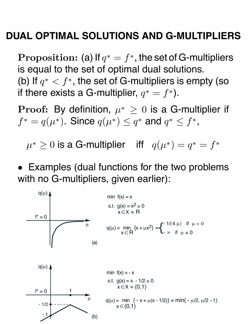
DUAL OPTIMAL SOLUTIONS AND G-MULTIPLIERS
Proposition: (a) If q∗ = f∗, the set of G-multipliersis equal to the set of optimal dual solutions.(b) If q∗ < f∗, the set of G-multipliers is empty (soif there exists a G-multiplier, q∗ = f∗).
Proof: By definition, µ∗ ≥ 0 is a G-multiplier iff∗ = q(µ∗). Since q(µ∗) ≤ q∗ and q∗ ≤ f∗,
µ∗ ≥ 0 is a G-multiplier iff q(µ∗) = q∗ = f∗
• Examples (dual functions for the two problemswith no G-multipliers, given earlier):
(a)
f* = 0
µ
q(µ)
1
(b)
µ
q(µ)
f* = 0
- 1
min f(x) = x
s.t. g(x) = x2 ≤ 0 x ∈ X = R
min f(x) = - x
s.t. g(x) = x - 1/2 ≤ 0 x ∈ X = {0,1}
q(µ) = min {x + µx2} ={- 1/(4 µ) if µ > 0
- ∞ if µ ≤ 0
- 1/2
x ∈ R
q(µ) = min { - x + µ(x - 1/2)} = min{ - µ/2, µ/2 −1} x ∈ {0,1}

DUALITY AND MINIMAX THEORY
• The primal and dual problems can be viewed interms of minimax theory:
Primal Problem <=> infx∈X
supµ≥0
L(x, µ)
Dual Problem <=> supµ≥0
infx∈X
L(x, µ)
• Optimality Conditions: (x∗, µ∗) is an optimalsolution/G-multiplier pair if and only if
x∗ ∈ X, g(x∗) ≤ 0, (Primal Feasibility),
µ∗ ≥ 0, (Dual Feasibility),
x∗ = arg minx∈X
L(x, µ∗), (Lagrangian Optimality),
µ∗jgj(x∗) = 0, j = 1, . . . , r, (Compl. Slackness).
• Saddle Point Theorem: (x∗, µ∗) is an opti-mal solution/G-multiplier pair if and only if x∗ ∈ X,µ∗ ≥ 0, and (x∗, µ∗) is a saddle point of the La-grangian, in the sense that
L(x∗, µ) ≤ L(x∗, µ∗) ≤ L(x, µ∗), ∀ x ∈ X, µ ≥ 0

A CONVEX PROBLEM WITH A DUALITY GAP
• Consider the two-dimensional problem
minimize f(x)subject to x1 ≤ 0, x ∈ X = {x | x ≥ 0},
where
f(x) = e−√
x1x2 , ∀ x ∈ X,
and f(x) is arbitrarily defined for x /∈ X.
• f is convex over X (its Hessian is positive defi-nite in the interior of X), and f∗ = 1.
• Also, for all µ ≥ 0 we have
q(µ) = infx≥0
{e−
√x1x2 + µx1
}= 0,
since the expression in braces is nonnegative forx ≥ 0 and can approach zero by taking x1 → 0and x1x2 → ∞. It follows that q∗ = 0.

INFEASIBLE AND UNBOUNDED PROBLEMS
0
min f(x) = 1/x
s.t. g(x) = x ≤ 0
x ∈ X = {x | x > 0}
(a)f* = ∞, q* = ∞
0
S = {(x2,x) | x > 0}
min f(x) = x
s.t. g(x) = x2 ≤ 0
x ∈ X = {x | x > 0}
(b)
f* = ∞, q* = 0
0
S = {(g(x),f(x)) | x ∈ X} = {(z,w) | z > 0}
min f(x) = x1 + x2s.t. g(x) = x1 ≤ 0
x ∈ X = {(x1,x2) | x1 > 0}
(c)f* = ∞, q* = −∞
z
w
w
w
z
z
S = {(g(x),f(x)) | x ∈ X}

LECTURE 19
LECTURE OUTLINE
• Linear and quadratic programming duality
• Conditions for existence of geometric multipliers
• Conditions for strong duality
−−−−−−−−−−−−−−−−−−−−−−−−−−−−• Primal problem: Minimize f(x) subject to x ∈ X,and g1(x) ≤ 0, . . . , gr(x) ≤ 0 (assuming −∞ <f∗ < ∞). It is equivalent to infx∈X supµ≥0 L(x, µ).
• Dual problem: Maximize q(µ) subject to µ ≥ 0,where q(µ) = infx∈X L(x, µ). It is equivalent tosupµ≥0 infx∈X L(x, µ).
• µ∗ is a geometric multiplier if and only if f∗ = q∗,and µ∗ is an optimal solution of the dual problem.
• Question: Under what conditions f∗ = q∗ andthere exists a geometric multiplier?

LINEAR AND QUADRATIC PROGRAMMING DUALITY
• Consider a LP or positive semidefinite QP underthe assumption
−∞ < f∗ < ∞
• We know from Chapter 2 that
−∞ < f∗ < ∞ ⇒ there is an optimal solution x∗
• Since the constraints are linear, there exist L-multipliers corresponding to x∗, so we can useLagrange multiplier theory.
• Since the problem is convex, the L-multiplierscoincide with the G-multipliers.
• Hence there exists a G-multiplier, f∗ = q∗ andthe optimal solutions of the dual problem coincidewith the Lagrange multipliers.

THE DUAL OF A LINEAR PROGRAM
• Consider the linear program
minimize c′x
subject to e′ix = di, i = 1, . . . , m, x ≥ 0
• Dual function
q(λ) = infx≥0
⎧⎨⎩
n∑j=1
(cj −
m∑i=1
λieij
)xj +
m∑i=1
λidi
⎫⎬⎭
• If cj −∑m
i=1 λieij ≥ 0 for all j, the infimumis attained for x = 0, and q(λ) =
∑mi=1 λidi. If
cj −∑m
i=1 λieij < 0 for some j, the expression inbraces can be arbitrarily small by taking xj suff.large, so q(λ) = −∞. Thus, the dual is
maximizem∑
i=1
λidi
subject tom∑
i=1
λieij ≤ cj , j = 1, . . . , n.

THE DUAL OF A QUADRATIC PROGRAM
• Consider the quadratic program
minimize 12x
′Qx + c′x
subject to Ax ≤ b,
where Q is a given n×n positive definite symmet-ric matrix, A is a given r × n matrix, and b ∈ �r
and c ∈ �n are given vectors.
• Dual function:
q(µ) = infx∈�n
{ 12x
′Qx + c′x + µ′(Ax − b)}
The infimum is attained for x = −Q−1(c + A′µ),and, after substitution and calculation,
q(µ) = − 12µ
′AQ−1A′µ−µ′(b+AQ−1c)− 12c
′Q−1c
• The dual problem, after a sign change, is
minimize 12µ
′Pµ + t′µ
subject to µ ≥ 0,
where P = AQ−1A′ and t = b + AQ−1c.

RECALL NONLINEAR FARKAS’ LEMMA
Let C ⊂ �n be convex, and f : C �→ � andgj : C �→ �, j = 1, . . . , r, be convex functions.Assume that
f(x) ≥ 0, ∀ x ∈ F ={x ∈ C | g(x) ≤ 0
},
and one of the following two conditions holds:
(1) 0 is in the relative interior of the setD =
{u | g(x) ≤ u for some x ∈ C
}.
(2) The functions gj , j = 1, . . . , r, are affine, andF contains a relative interior point of C.
Then, there exist scalars µ∗j ≥ 0, j = 1, . . . , r, s. t.
f(x) +r∑
j=1
µ∗jgj(x) ≥ 0, ∀ x ∈ C

APPLICATION TO CONVEX PROGRAMMING
Consider the problem
minimize f(x)subject to x ∈ C, gj(x) ≤ 0, j = 1, . . . , r,
where C, f : C �→ �, and gj : C �→ � are convex.Assume that the optimal value f∗ is finite.
• Replace f(x) by f(x)−f∗ and assume that theconditions of Farkas’ Lemma are satisfied. Thenthere exist µ∗
j ≥ 0 such that
f∗ ≤ f(x) +r∑
j=1
µ∗jgj(x), ∀ x ∈ C
Since F ⊂ C and µ∗jgj(x) ≤ 0 for all x ∈ F ,
f∗ ≤ infx∈F
⎧⎨⎩f(x) +
r∑j=1
µ∗jgj(x)
⎫⎬⎭ ≤ inf
x∈Ff(x) = f∗
Thus equality holds throughout, we have
f∗ = infx∈C
{f(x) + µ∗′g(x)} ,
and µ∗ is a geometric multiplier.

STRONG DUALITY THEOREM I
Assumption : (Convexity and Linear Constraints)f∗ is finite, and the following hold:
(1) X = P ∩ C, where P is polyhedral and C isconvex.
(2) The cost function f is convex over C and thefunctions gj are affine.
(3) There exists a feasible solution of the prob-lem that belongs to the relative interior of C.
Proposition : Under the above assumption, thereexists at least one geometric multiplier.
Proof: If P = �n the result holds by Farkas. IfP �= �n, express P as
P = {x | a′jx − bj ≤ 0, j = r + 1, . . . , p}
Apply Farkas to the extended representation, with
F = {x ∈ C | a′jx − bj ≤ 0, j = 1, . . . , p}
Assert the existence of geometric multipliers inthe extended representation, and pass back to theoriginal representation. Q.E.D.

STRONG DUALITY THEOREM II
Assumption : (Linear and Nonlinear Constraints)f∗ is finite, and the following hold:
(1) X = P ∩ C, with P : polyhedral, C: convex.
(2) The functions f and gj , j = 1, . . . , r, areconvex over C, and the functions gj , j =r + 1, . . . , r, are affine.
(3) There exists a feasible vector x such thatgj(x) < 0 for all j = 1, . . . , r.
(4) There exists a vector that satisfies the lin-ear constraints [but not necessarily the con-straints gj(x) ≤ 0, j = 1, . . . , r] and belongsto the relative interior of C.
Proposition : Under the above assumption, thereexists at least one geometric multiplier.
Proof: If P = �n and there are no linear con-straints (the Slater condition), apply Farkas. Oth-erwise, lump the linear constraints within X, as-sert the existence of geometric multipliers for thenonlinear constraints, then use the preceding du-ality result for linear constraints. Q.E.D.

THE PRIMAL FUNCTION
• Minimax theory centered around the function
p(u) = infx∈X
supµ≥0
{L(x, µ) − µ′u
}• Properties of p around u = 0 are critical in an-alyzing the presence of a duality gap and the ex-istence of primal and dual optimal solutions.
• p is known as the primal function of the con-strained optimization problem.
• We have
supµ≥0
{L(x, µ) − µ′u
}= sup
µ≥0
{f(x) + µ′
(g(x) − u
)}=
{f(x) if g(x) ≤ u,∞ otherwise.• So
p(u) = infx∈X
g(x)≤u
f(x)
and p(u) can be viewed as a perturbed optimalvalue [note that p(0) = f∗].

CONDITIONS FOR NO DUALITY GAP
• Apply the minimax theory specialized to L(x, µ).
• Assume that f∗ < ∞, and that X is convex, andL(·, µ) is convex over X for each µ ≥ 0. Then:
− p is convex.
− There is no duality gap if and only if p is lowersemicontinuous at u = 0.
• Conditions that guarantee lower semicontinuityat u = 0, correspond to those for preservation ofclosure under partial minimization, e.g.:
− f∗ < ∞, X is convex and compact, and foreach µ ≥ 0, the function L(·, µ), restricted tohave domain X, is closed and convex.
− Extensions involving directions of recessionof X, f , and gj , and guaranteeing that theminimization in p(u) = inf x∈X
g(x)≤uf(x) is (ef-
fectively) over a compact set.
• Under the above conditions, there is no dualitygap, and the primal problem has a nonempty andcompact optimal solution set. Furthermore, theprimal function p is closed, proper, and convex.

LECTURE 20
LECTURE OUTLINE
• The primal function
• Conditions for strong duality
• Sensitivity
• Fritz John conditions for convex programming−−−−−−−−−−−−−−−−−−−−−−−−−−−−• Problem: Minimize f(x) subject to x ∈ X, andg1(x) ≤ 0, . . . , gr(x) ≤ 0 (assuming −∞ < f∗ <∞). It is equivalent to infx∈X supµ≥0 L(x, µ).
• The primal function is the perturbed optimalvalue
p(u) = infx∈X
supµ≥0
{L(x, µ) − µ′u
}= inf
x∈Xg(x)≤u
f(x)
• Note that p(u) is the result of partial minimizationover X of the function F (x, u) given by
F (x, u) ={
f(x) if x ∈ X and g(x) ≤ u,∞ otherwise.

PRIMAL FUNCTION AND STRONG DUALITY
• Apply min common-max crossing frameworkwith set M = epi(p), assuming p is convex and−∞ < p(0) < ∞.
• There is no duality gap if and only if p is lowersemicontinuous at u = 0.
• Conditions that guarantee lower semicontinuityat u = 0, correspond to those for preservationof closure under the partial minimization p(u) =inf x∈X
g(x)≤uf(x), e.g.:
− X is convex and compact, f, gj : convex.
− Extensions involving the recession cones ofX, f , gj .
− X = �n, f, gj : convex quadratic.

RELATION OF PRIMAL AND DUAL FUNCTIONS
• Consider the dual function q. For every µ ≥ 0,we have
q(µ) = infx∈X
{f(x) + µ′g(x)}
= inf{(u,x)|x∈X, g(x)≤u, j=1,...,r}
{f(x) + µ′g(x)}
= inf{(u,x)|x∈X, g(x)≤u}
{f(x) + µ′u}
= infu∈�r
infx∈X, g(x)≤u
{f(x) + µ′u} .
• Thus
q(µ) = infu∈�r
{p(u) + µ′u
}, ∀ µ ≥ 0
S={(g(x),f(x)) | x ∈ X}
f*
u
w
q* p(u)
q(µ) = infu{p(u) + µ′u}
(µ,1)

SUBGRADIENTS OF THE PRIMAL FUNCTION
S ={(g(x),f(x)) | x ∈ X}
u
p(u)f*
0
Slope: -µ*
(µ*,1)
• Assume that p is convex, p(0) is finite, and p isproper. Then:
− The set of G-multipliers is −∂p(0) (negativesubdifferential of p at u = 0). This followsfrom the relation
q(µ) = infu∈�r
{p(u) + µ′u
}
− If the origin lies in the relative interior of theeffective domain of p, then there exists a G-multiplier.
− If the origin lies in the interior of the effec-tive domain of p, the set of G-multipliers isnonempty and compact.

SENSITIVITY ANALYSIS I
• Assume that p is convex and differentiable.Then −∇p(0) is the unique G-multiplier µ∗, andwe have
µ∗j = −∂p(0)
∂uj, ∀ j
• Let µ∗ be a G-multiplier, and consider a vectoruγ
j of the form
uγj = (0, . . . , 0, γ, 0, . . . , 0)
where γ is a scalar in the jth position. Then
limγ↑0
p(uγj ) − p(0)
γ≤ −µ∗
j ≤ limγ↓0
p(uγj ) − p(0)
γ
Thus −µ∗j lies between the left and the right slope
of p in the direction of the jth axis starting at u = 0.

SENSITIVITY ANALYSIS II
• Assume that p is convex and finite in a neighbor-hood of 0. Then, from the theory of subgradients:
− ∂p(0) is nonempty and compact.
− The directional derivative p′(0; y) is a real-valued convex function of y satisfying
p′(0; y) = maxg∈∂p(0)
y′g
• Consider the direction of steepest descent of pat 0, i.e., the y that minimizes p′(0; y) over ‖y‖ ≤ 1.Using the Saddle Point Theorem,
p′(0; y) = min‖y‖≤1
p′(0; y) = min‖y‖≤1
maxg∈∂p(0)
y′g = maxg∈∂p(0)
min‖y‖≤1
y′g
• The saddle point is (g∗, y), where g∗ is thesubgradient of minimum norm in ∂p(0) and y =−g∗/‖g∗‖. The min-max value is −‖g∗‖.
• Conclusion: If µ∗ is the G-multiplier of mini-mum norm and µ∗ �= 0, the direction of steepestdescent of p at 0 is y = µ∗/‖µ∗‖, while the rateof steepest descent (per unit norm of constraintviolation) is ‖µ∗‖.

FRITZ JOHN THEORY FOR CONVEX PROBLEMS
• Assume that X is convex, the functions f andgj are convex over X, and f∗ < ∞. Then thereexist a scalar µ∗
0 and a vector µ∗ = (µ∗1, . . . , µ
∗r)
satisfying the following conditions:
(i) µ∗0f
∗ = infx∈X
{µ∗
0f(x) + µ∗′g(x)}
.
(ii) µ∗j ≥ 0 for all j = 0, 1, . . . , r.
(iii) µ∗0, µ
∗1, . . . , µ
∗r are not all equal to 0.
(0,f*)
(µ∗,µ0∗)
w
u
M = {(u,w) | there is an x ∈ X such that g(x) ≤ u, f(x) ≤ w}
S = {(g(x),f(x)) | x ∈ X}
• If the multiplier µ∗0 can be proved positive, then
µ∗/µ∗0 is a G-multiplier.
• Under the Slater condition (there exists x ∈ Xs.t. g(x) < 0), µ∗
0 cannot be 0; if it were, then0 = infx∈X µ∗′g(x) for some µ∗ ≥ 0 with µ∗ �= 0,while we would also have µ∗′g(x) < 0.

FRITZ JOHN THEORY FOR LINEAR CONSTRAINTS
• Assume that X is convex, f is convex over X,the gj are affine, and f∗ < ∞. Then there exist ascalar µ∗
0 and a vector µ∗ = (µ∗1, . . . , µ
∗r), satisfy-
ing the following conditions:
(i) µ∗0f
∗ = infx∈X
{µ∗
0f(x) + µ∗′g(x)}
.
(ii) µ∗j ≥ 0 for all j = 0, 1, . . . , r.
(iii) µ∗0, µ
∗1, . . . , µ
∗r are not all equal to 0.
(iv) If the index set J = {j �= 0 | µ∗j > 0} is
nonempty, there exists a vector x ∈ X suchthat f(x) < f∗ and µ∗′
g(x) > 0.
• Proof uses Polyhedral Proper Separation Th.
• Can be used to show that there exists a geomet-ric multiplier if X = P ∩C, where P is polyhedral,and ri(C) contains a feasible solution.
• Conclusion: The Fritz John theory is suffi-ciently powerful to show the major constraint qual-ification theorems for convex programming.
• The text has more material on pseudonormality,informative geometric multipliers, etc.

LECTURE 21
LECTURE OUTLINE
• Fenchel Duality
• Conjugate Convex Functions
• Relation of Primal and Dual Functions
• Fenchel Duality Theorems
−−−−−−−−−−−−−−−−−−−−−−−−−−−−

FENCHEL DUALITY FRAMEWORK
• Consider the problem
minimize f1(x) − f2(x)subject to x ∈ X1 ∩ X2,
where f1 and f2 are real-valued functions on �n,and X1 and X2 are subsets of �n.
• Assume that f∗ < ∞.
• Convert problem to
minimize f1(y) − f2(z)subject to z = y, y ∈ X1, z ∈ X2,
and dualize the constraint z = y:
q(λ) = infy∈X1, z∈X2
{f1(y) − f2(z) + (z − y)′λ
}= inf
z∈X2
{z′λ − f2(z)
}− sup
y∈X1
{y′λ − f1(y)
}= g2(λ) − g1(λ)

CONJUGATE FUNCTIONS
• The functions g1(λ) and g2(λ) are called theconjugate convex and conjugate concave functionscorresponding to the pairs (f1, X1) and (f2, X2).
• An equivalent definition of g1 is
g1(λ) = supx∈�n
{x′λ − f1(x)
},
where f1 is the extended real-valed function
f1(x) ={
f1(x) if x ∈ X1,∞ if x /∈ X1.
• We are led to consider the conjugate convexfunction of a general extended real-valued properfunction f : �n �→ (−∞,∞]:
g(λ) = supx∈�n
{x′λ − f(x)
}, λ ∈ �n.
• Conjugate concave functions are defined throughconjugate convex functions after appropriate signreversals.

VISUALIZATION
g(λ) = supx∈�n
{x′λ − f(x)
}, λ ∈ �n
0x
f(x)
(- λ,1)
inf {f(x) - x'λ} = - g(λ)x
x'λ - g(λ)
f(x) = sup { x'λ - g(λ)}~
λ
(a)
0
f(x)
f(x) = sup { x'λ - g(λ)}~
λ
Conjugate ofconjugate of f
(b)

EXAMPLES OF CONJUGATE PAIRS
g(λ) = supx∈�n
{x′λ−f(x)
}, f(x) = sup
λ∈�n
{x′λ−g(λ)
}
0 x
Slope = α
β/α 0 λα
β
g(λ) = { β if λ = α∞ if λ ≠ αf(x) = αx - β
0 x 0 λ
g(λ) = {0 if |λ| ≤ 1∞ if |λ| > 1
f(x) = |x|
0 x 0 λ
g(λ) = (1/2c)λ2f(x) = (c/2)x2
X = (- ∞, ∞)
X = (- ∞, ∞)
X = (- ∞, ∞)
1-1

CONJUGATE OF THE CONJUGATE FUNCTION
• Two cases to consider:
− f is a closed proper convex function.
− f is a general extended real-valued properfunction.
• We will see that for closed proper convex func-tions, the conjugacy operation is symmetric, i.e.,the congugate of f is a closed proper convex func-tion, and the conjugate of the conjugate is f .
• Leads to a symmetric/dual Fenchel duality theo-rem for the case where the functions involved areclosed convex/concave.
• The result can be generalized:
− The convex closure of f , is the function thathas as epigraph the closure of the convexhull if epi(f) [also the smallest closed andconvex set containing epi(f)].
− The epigraph of the convex closure of f isthe intersection of all closed halfspaces of�n+1 that contain the epigraph of f .

CONJUGATE FUNCTION THEOREM
• Let f : �n �→ (−∞,∞] be a function, let f beits convex closure, let g be its convex conjugate,and consider the conjugate of g,
f(x) = supλ∈�n
{λ′x − g(λ)
}, x ∈ �n
(a) We have
f(x) ≥ f(x), ∀ x ∈ �n
(b) If f is convex, then properness of any one off , g, and f implies properness of the othertwo.
(c) If f is closed proper and convex, then
f(x) = f(x), ∀ x ∈ �n
(d) If f(x) > −∞ for all x ∈ �n, then
f(x) = f(x), ∀ x ∈ �n

CONJUGACY OF PRIMAL AND DUAL FUNCTIONS
• Consider the problem
minimize f(x)subject to x ∈ X, gj(x) ≤ 0, j = 1, . . . , r.
• We showed in the previous lecture the followingrelation between primal and dual functions:
q(µ) = infu∈�r
{p(u) + µ′u
}, ∀ µ ≥ 0.
• Thus, q(µ) = − supu∈�r
{−µ′u − p(u)
}or
q(µ) = −h(−µ), ∀ µ ≥ 0,
where h is the conjugate convex function of p:
h(ν) = supu∈�r
{ν′u − p(u)
}

INDICATOR AND SUPPORT FUNCTIONS
• The indicator function of a nonempty set is
δX(x) ={ 0 if x ∈ X,∞ if x /∈ X.
• The conjugate of δX , given by
σX(λ) = supx∈X
λ′x,
is called the support function of X.
• X has the same support function as cl(conv(X)
)(by the Conjugacy Theorem).
• If X is closed and convex, δX is closed and con-vex, and by the Conjugacy Theorem the conjugateof its support function is its indicator function.
• The support function satisfies
σX(αλ) = ασX(λ), ∀ α > 0, ∀ λ ∈ �n
so its epigraph is a cone. Functions with this prop-erty are called positively homogeneous.

MORE ON SUPPORT FUNCTIONS
• For a cone C, we have
σC(λ) = supx∈C
λ′x ={
0 if λ ∈ C∗,∞ otherwise,
i.e., the support function of a cone is the indicatorfunction of its polar.
• The support function of a polyhedral set is apolyhedral function that is pos. homogeneous. Theconjugate of a pos. homogeneous polyhedral func-tion is the support function of some polyhedral set.
• A function can be equivalently specified in termsof its epigraph. As a consequence, we will seethat the conjugate of a function can be specifiedin terms of the support function of its epigraph.
• The conjugate of f , can equivalently be writtenas g(λ) = sup(x,w)∈epi(f)
{x′λ − w
}, so
g(λ) = σepi(f)(λ,−1), ∀ λ ∈ �n
• From this formula, we also obtain that the con-jugate of a polyhedral function is polyhedral.

LECTURE 22
LECTURE OUTLINE
• Fenchel Duality
• Fenchel Duality Theorems
• Cone Programming
• Semidefinite Programming
−−−−−−−−−−−−−−−−−−−−−−−−−−−−• Recall the conjugate convex function of a gen-eral extended real-valued proper function f : �n �→(−∞,∞]:
g(λ) = supx∈�n
{x′λ − f(x)
}, λ ∈ �n.
• Conjugacy Theorem: If f is closed and con-vex, then f is equal to the 2nd conjugate (the con-jugate of the conjugate).

FENCHEL DUALITY FRAMEWORK
• Consider the problem
minimize f1(x) − f2(x)subject to x ∈ X1 ∩ X2,
where f1 : �n �→ (−∞,∞] and f2 : �n �→ [−∞,∞).
• Assume that f∗ < ∞.
• Convert problem to
minimize f1(y) − f2(z)subject to z = y, y ∈ dom(f1), z ∈ dom(−f2),
and dualize the constraint z = y:
q(λ) = infy∈�n, z∈�n
{f1(y) − f2(z) + (z − y)′λ
}= inf
z∈�n
{z′λ − f2(z)
}− sup
y∈�n
{y′λ − f1(y)
}= g2(λ) − g1(λ)

FENCHEL DUALITY THEOREM
0 x 0 x
dom(f1)
f1(x)
(- λ,1)
(- λ,1)
Slope = λ
inf {f1(x) - x'λ} = - g1(λ)x
sup {f2(x) - x'λ} = - g2(λ)x
f2(x)
Slope = λ
dom(-f2)
• Assume thatf1 and f2 are convex and concave,respectively. If either
− The relative interiors of dom(f1) and dom(−f2)intersect, or
− dom(f1) and dom(−f2) are polyhedral, andf1 and f2 can be extended to real-valuedconvex and concave functions over �n.
Then the geometric multipliers existence theoremapplies and we have
f∗ = maxλ∈�n
{g2(λ) − g1(λ)
},
while the maximum above is attained.

OPTIMALITY CONDITIONS
• There is no duality gap, while (x∗, λ∗) is anoptimal primal and dual solution pair, if and only if
x∗ ∈ dom(f1)∩dom(−f2), (primal feasibility),
λ∗ ∈ dom(g1) ∩ dom(−g2), (dual feasibility),
x∗ = arg maxx∈�n
{x′λ∗ − f1(x)
}= arg min
x∈�n
{x′λ∗ − f2(x)
}, (Lagr. optimality).
0 x
f1(x)
Slope = λg2(λ) - g1(λ)
x*
f2(x)
Slope = λ*
g2(λ*) - g1(λ*)
(- λ*,1)
(- λ,1)
• Note: The Lagrangian optimality condition isequivalent to λ∗ ∈ ∂f1(x∗) ∩ ∂f1(x∗).

DUAL FENCHEL DUALITY THEOREM
• The dual problem
maxλ∈�n
{g2(λ) − g1(λ)
}is of the same form as the primal.
• By the conjugacy theorem, if the functions f1
and f2 are closed, in addition to being convex andconcave, they are the conjugates of g1 and g2.
• Conclusion: The primal problem has an opti-mal solution, there is no duality gap, and we have
minx∈�n
{f1(x) − f2(x)
}= sup
λ∈�n
{g2(λ) − g1(λ)
},
if either
− The relative interiors of dom(g1) and dom(−g2)intersect, or
− dom(g1) and dom(−g2) are polyhedral, andg1 and g2 can be extended to real-valuedconvex and concave functions over �n.

CONIC DUALITY I
• Consider the problem
minimize f(x)subject to x ∈ C,
where C is a convex cone, and f : �n �→ (−∞,∞]is convex.
• Apply Fenchel duality with the definitions
f1(x) = f(x), f2(x) ={
0 if x ∈ C,−∞ if x /∈ C.
We have
g1(λ) = supx∈�n
{λ′x−f(x)
}, g2(λ) = inf
x∈C
x′λ =
{0 if λ ∈ C,
−∞ if λ /∈ C,
where C is the negative polar cone (sometimescalled the dual cone of C):
C = −C∗ = {λ | x′λ ≥ 0, ∀ x ∈ C}

CONIC DUALITY II
• Fenchel duality can be written as
infx∈C
f(x) = supλ∈C
−g(λ),
where g(λ) is the conjugate of f .
• By the Primal Fenchel Theorem, there is noduality gap and the sup is attained if one of thefollowing holds:
(a) ri(dom(f)) ∩ ri(C) �= Ø.
(b) f can be extended to a real-valued convexfunction over �n, and dom(f) and C arepolyhedral.
• Similarly, by the Dual Fenchel Theorem, if f isclosed and C is closed, there is no duality gapand the infimum in the primal problem is attainedif one of the following two conditions holds:
(a) ri(dom(g)) ∩ ri(C) �= Ø.
(b) g can be extended to a real-valued convexfunction over�n, and dom(g) and C are poly-hedral.

THE AFFINE COST CASE OF CONIC DUALITY
• Let f be affine, f(x) = c′x, with dom(f) being anaffine set, dom(f) = b+S, where S is a subspace.
• The primal problem is
minimize c′x
subject to x − b ∈ S, x ∈ C.
• The conjugate is
g(λ) = supx−b∈S
(λ − c)′x = supy∈S
(λ − c)′(y + b)
={
(λ − c)′b if λ − c ∈ S⊥,∞ if λ − c /∈ S⊥,
so the dual problem is
minimize b′λ
subject to λ − c ∈ S⊥, λ ∈ C.
• The primal and dual have the same form.
• If C is closed, the dual of the dual yields theprimal.

SEMIDEFINITE PROGRAMMING: A SPECIAL CASE
• Consider the symmetric n × n matrices. Innerproduct < X, Y >= trace(XY ) =
∑ni,j=1 xijyij .
• Let D be the cone of pos. semidefinite matrices.Note that D is self-dual [D = D, i.e., < X, Y >≥ 0for all y ∈ D iff X ∈ D], and its interior is the setof pos. definite matrices.
• Fix symmetric matrices C, A1, . . . , Am, and vec-tors b1, . . . , bm, and consider
minimize < C, X >
subject to < Ai, X >= bi, i = 1, . . . , m, X ∈ D
• Viewing this as an affine cost conic problem,the dual problem (after some manipulation) is
maximizem∑
i=1
biλi
subject to C − (λ1A1 + · · · + λmAm) ∈ D.
• There is no duality gap if there exists λ suchthat C − (λ1A1 + · · · + λmAm) is pos. definite.

LECTURE 23
LECTURE OUTLINE
• Overview of Dual Methods
• Nondifferentiable Optimization
********************************
• Consider the primal problem
minimize f(x)subject to x ∈ X, gj(x) ≤ 0, j = 1, . . . , r,
assuming −∞ < f∗ < ∞.
• Dual problem: Maximize
q(µ) = infx∈X
L(x, µ) = infx∈X
{f(x) + µ′g(x)}
subject to µ ≥ 0.

PROS AND CONS FOR SOLVING THE DUAL
• The dual is concave.
• The dual may have smaller dimension and/orsimpler constraints.
• If there is no duality gap and the dual is solvedexactly for a geometric multiplier µ∗, all optimalprimal solutions can be obtained by minimizingthe Lagrangian L(x, µ∗) over x ∈ X.
• Even if there is a duality gap, q(µ) is a lowerbound to the optimal primal value for every µ ≥ 0.
• Evaluating q(µ) requires minimization of L(x, µ)over x ∈ X.
• The dual function is often nondifferentiable.
• Even if we find an optimal dual solution µ∗, itmay be difficult to obtain a primal optimal solution.

FAVORABLE STRUCTURE
• Separability: Classical duality structure (La-grangian relaxation).
• Partitioning: The problem
minimize F (x) + G(y)subject to Ax + By = c, x ∈ X, y ∈ Y
can be written as
minimize F (x) + infBy=c−Ax, y∈Y
G(y)
subject to x ∈ X.
With no duality gap, this problem is written as
minimize F (x) + Q(Ax)subject to x ∈ X,
whereQ(Ax) = max
λq(λ, Ax)
q(λ, Ax) = infy∈Y
{G(y) + λ′(Ax + By − c)
}

DUAL DERIVATIVES
• Let
xµ = arg minx∈X
L(x, µ) = arg minx∈X
{f(x) + µ′g(x)
}Then for all µ ∈ �r,
q(µ) = infx∈X
{f(x) + µ′g(x)
}≤ f(xµ) + µ′g(xµ)= f(xµ) + µ′g(xµ) + (µ − µ)′g(xµ)= q(µ) + (µ − µ)′g(xµ).
• Thus g(xµ) is a subgradient of q at µ.
• Proposition: Let X be compact, and let f andg be continuous over X. Assume also that for ev-ery µ, L(x, µ) is minimized over x ∈ X at a uniquepoint xµ. Then, q is everywhere continuously dif-ferentiable and
∇q(µ) = g(xµ), ∀ µ ∈ �r

NONDIFFERENTIABILITY OF THE DUAL
• If there exists a duality gap, the dual functionis nondifferentiable at every dual optimal solution(see the textbook).
• Important nondifferentiable case: When q ispolyhedral, that is,
q(µ) = mini∈I
{a′
iµ + bi
},
where I is a finite index set, and ai ∈ �r and bi
are given (arises when X is a discrete set, as ininteger programming).
• Proposition: Let q be polyhedral as above,and let Iµ be the set of indices attaining the mini-mum
Iµ ={i ∈ I | a′
iµ + bi = q(µ)}
The set of all subgradients of q at µ is
∂q(µ) =
⎧⎨⎩g
∣∣∣ g =∑i∈Iµ
ξiai, ξi ≥ 0,∑i∈Iµ
ξi = 1
⎫⎬⎭

NONDIFFERENTIABLE OPTIMIZATION
• Consider maximization of q(µ) over M = {µ ≥0 | q(µ) > −∞}• Subgradient method:
µk+1 =[µk + skgk
]+,
where gk is the subgradient g(xµk), [·]+ denotesprojection on the closed convex set M , and sk isa positive scalar stepsize.
M
gk
µk
µk + skgk
[µk + skgk]+
µ*
Contours of q

KEY SUBGRADIENT METHOD PROPERTY
• For a small stepsize it reduces the Euclideandistance to the optimum.
M
gk
µk
µk + skgk
µk+1 = [µk + skgk]+µ*
< 90o
Contours of q
• Proposition: For any dual optimal solution µ∗,we have
‖µk+1 − µ∗‖ < ‖µk − µ∗‖,
for all stepsizes sk such that
0 < sk <2(q(µ∗) − q(µk)
)‖gk‖2

STEPSIZE RULES
• Constant stepsize: sk ≡ s for some s > 0.
• If ‖gk‖ ≤ C for some constant C and all k,
‖µk+1−µ∗‖2 ≤ ‖µk−µ∗‖2−2s(q(µ∗)−q(µk)
)+s2C2,
so the distance to the optimum decreases if
0 < s <2(q(µ∗) − q(µk)
)C2
or equivalently, if µk belongs to the level set
{µ
∣∣∣ q(µ) < q(µ∗) − sC2
2
}
• With a little further analysis, it can be shownthat the method, at least asymptotically, reachesthis level set, i.e.
lim supk→∞
q(µk) ≥ q(µ∗) − sC2
2

OTHER STEPSIZE RULES
• Diminishing stepsize: sk → 0 with some restric-tions.
• Dynamic stepsize rule (involves a scalar se-quence {qk}):
sk =αk
(qk − q(µk)
)‖gk‖2
,
where qk ≈ q∗ and 0 < αk < 2.
• Some possibilities:
− qk is the best known upper bound to q∗: startwith α0 = 1 and decrease αk by a certainfactor every few iterations.
− αk = 1 for all k and
qk =(1 + β(k)
)qk,
where qk = max0≤i≤k q(µi), and β(k) > 0 isadjusted depending on algorithmic progressof the algorithm.

LECTURE 24
LECTURE OUTLINE
• Subgradient Methods
• Stepsize Rules and Convergence Analysis
********************************
• Consider a generic convex problem minx∈X f(x),where f : �n �→ � is a convex function and X isa closed convex set, and the subgradient method
xk+1 = [xk − αkgk]+ ,
where gk is a subgradient of f at xk, αk is a positivestepsize, and [·]+ denotes projection on the set X.
• Incremental version for problem minx∈X
∑mi=1 fi(x)
xk+1 = ψm,k, ψi,k = [ψi−1,k − αkgi,k]+ , i = 1, . . . , m
starting with ψ0,k = xk, where gi,k is a subgradientof fi at ψi−1,k.

ASSUMPTIONS AND KEY INEQUALITY
• Assumption: (Subgradient Boundedness)
||g|| ≤ Ci, ∀ g ∈ ∂fi(xk)∪∂fi(ψi−1,k), ∀ i, k,
for some scalars C1, . . . , Cm. (Satisfied when thefi are polyhedral as in integer programming.)
• Key Lemma: For all y ∈ X and k,
||xk+1−y||2 ≤ ||xk−y||2−2αk
(f(xk)−f(y)
)+α2
kC2,
where
C =m∑
i=1
Ci
and Ci is as in the boundedness assumption.
• Note: For any y that is better than xk, the dis-tance to y is improved if αk is small enough:
0 < αk <2(f(xk) − f(y)
)C2

PROOF OF KEY LEMMA
• For each fi and all y ∈ X, and i, k
||ψi,k − y||2 = ||[ψi−1,k − αkgi,k]+ − y||2≤ ||ψi−1,k − αkgi,k − y||2≤ ||ψi−1,k − y||2 − 2αkg′i,k(ψi−1,k − y) + α2
kC2i
≤ ||ψi−1,k − y||2 − 2αk
(fi(ψi−1,k) − fi(y)
)+ α2
kC2i
By adding over i, and strengthening,
||xk+1 − y||2 ≤ ||xk − y||2 − 2αk
(f(xk) − f(y)
)+ 2αk
m∑i=1
Ci||ψi−1,k − xk|| + α2k
m∑i=1
C2i
≤ ||xk − y||2 − 2αk
(f(xk) − f(y)
)+ α2
k
⎛⎝2
m∑i=2
Ci
⎛⎝i−1∑
j=1
Cj
⎞⎠ +
m∑i=1
C2i
⎞⎠
= ||xk − y||2 − 2αk
(f(xk) − f(y)
)+ α2
k
(m∑
i=1
Ci
)2
= ||xk − y||2 − 2αk
(f(xk) − f(y)
)+ α2
kC2.

STEPSIZE RULES
• Constant Stepsize αk ≡ α:
− By key lemma with f(y) ≈ f∗, it makes progress
to the optimal if 0 < α <2(f(xk)−f∗
)C2 , i.e., if
f(xk) > f∗ +αC2
2
• Diminishing Stepsize αk → 0,∑
k αk = ∞:
− Eventually makes progress (once αk becomessmall enough). Can show that
lim infk→∞
f(xk) = f∗
• Dynamic Stepsize αk = f(xk)−fk
C2 where fk = f∗
or (more practically) an estimate of f∗:
− If fk = f∗, makes progress at every iteration.If fk < f∗ it tends to oscillate around theoptimum. If fk > f∗ it tends towards thelevel set {x | f(x) ≤ fk}.

CONSTANT STEPSIZE ANALYSIS
• Proposition: For αk ≡ α, we have
lim infk→∞
f(xk) ≤ f∗ +αC2
2,
where C =∑m
i=1 Ci (in the case where f∗ = −∞,we have lim infk→∞ f(xk) = −∞.)
• Proof by contradiction. Let ε > 0 be s.t.
lim infk→∞
f(xk) > f∗ +αC2
2+ 2ε,
and let y ∈ X be such that
lim infk→∞
f(xk) ≥ f(y) +αC2
2+ 2ε
For all k large enough, we have
f(xk) ≥ lim infk→∞
f(xk) − ε
Add to get f(xk)−f(y) ≥ αC2/2+ ε. Use the keylemma for y = y to obtain a contradiction.

COMPLEXITY ESTIMATE FOR CONSTANT STEP
• For any ε > 0, we have
min0≤k≤K
f(xk) ≤ f∗ +αC2 + ε
2
where
K =
⌊(d(x0, X∗)
)2
αε
⌋
• By contradiction. Assume that for 0 ≤ k ≤ K
f(xk) > f∗ +αC2 + ε
2
Using this relation in the key lemma,
(d(xk+1, X
∗))2 ≤
(d(xk, X∗)
)2
− 2α(f(xk) − f∗)+α2C2
≤(d(xk, X∗)
)2 − (α2C2 + αε) + α2C2
=(d(xk, X∗)
)2 − αε.
Sum over k to get(d(x0, X∗)
)2 − (K + 1)αε ≥ 0.

CONVERGENCE FOR OTHER STEPSIZE RULES
• (Diminishing Step): Assume that
αk > 0, limk→∞
αk = 0,∞∑
k=0
αk = ∞
Then,lim infk→∞
f(xk) = f∗
If the set of optimal solutions X∗ is nonempty andcompact,
limk→∞
d(xk, X∗) = 0, limk→∞
f(xk) = f∗
• (Dynamic Stepsize with fk = f∗): If X∗ isnonempty, xk converges to some optimal solution.

DYNAMIC STEPSIZE WITH ESTIMATE
• Estimation method:
f levk = min
0≤j≤kf(xj) − δk,
and δk is updated according to
δk+1 ={
ρδk if f(xk+1) ≤ f levk ,
max{βδk, δ
}if f(xk+1) > f lev
k ,
where δ, β, and ρ are fixed positive constants withβ < 1 and ρ ≥ 1.
• Here we essentially “aspire” to reach a tar-get level that is smaller by δk over the best valueachieved thus far.
• We can show that
infk≥0
f(xk) ≤ f∗ + δ
(or infk≥0 f(xk) = f∗ if f∗ = −∞).

LECTURE 25
LECTURE OUTLINE
• Incremental Subgradient Methods
• Convergence Rate Analysis and RandomizedMethods
********************************
• Incremental subgradient method for problemminx∈X
∑mi=1 fi(x)
xk+1 = ψm,k, ψi,k = [ψi−1,k − αkgi,k]+ , i = 1, . . . , m
starting with ψ0,k = xk, where gi,k is a subgradientof fi at ψi−1,k.
• Key Lemma: For all y ∈ X and k,
||xk+1−y||2 ≤ ||xk−y||2−2αk
(f(xk)−f(y)
)+α2
kC2,
where C =∑m
i=1 Ci and
Ci = supk
{||g|| | g ∈ ∂fi(xk) ∪ ∂fi(ψi−1,k)
}

CONSTANT STEPSIZE
• For αk ≡ α, we have
lim infk→∞
f(xk) ≤ f∗ +αC2
2
• Sharpness of the estimate:
− Consider the problem
minx
M∑i=1
C0
(|x + 1| + 2|x| + |x − 1|
)
with the worst component processing order
• Lower bound on the error. There is a problem,where even with best processing order,
f∗ +αmC2
0
2≤ lim inf
k→∞f(xk)
whereC0 = max{C1, . . . , Cm}

COMPLEXITY ESTIMATE FOR CONSTANT STEP
• For any ε > 0, we have
min0≤k≤K
f(xk) ≤ f∗ +αC2 + ε
2
where
K =
⌊(d(x0, X∗)
)2
αε
⌋

RANDOMIZED ORDER METHODS
xk+1 =[xk − αkg(ωk, xk)
]+where ωk is a random variable taking equiprobablevalues from the set {1, . . . , m}, and g(ωk, xk) is asubgradient of the component fωk at xk.
• Assumptions:
(a) {ωk} is a sequence of independent randomvariables. Furthermore, the sequence {ωk}is independent of the sequence {xk}.
(b) The set of subgradients{g(ωk, xk) | k =
0, 1, . . .}
is bounded, i.e., there exists a pos-itive constant C0 such that with prob. 1
||g(ωk, xk)|| ≤ C0, ∀ k ≥ 0
• Stepsize Rules:
− Constant: αk ≡ α
− Diminishing:∑
k αk = ∞,∑
k(αk)2 < ∞− Dynamic

RANDOMIZED METHOD W/ CONSTANT STEP
• With probability 1
infk≥0
f(xk) ≤ f∗ +αmC2
0
2
(with infk≥0 f(xk) = −∞ when f∗ = −∞).
Proof: By adapting key lemma, for all y ∈ X, k
||xk+1−y||2 ≤ ||xk−y||2−2α(fωk(xk)−fωk(y)
)+α2C2
0
Take conditional expectation withFk = {x0, . . . , xk}
E{||xk+1 − y||2 | Fk
}≤ ||xk − y||2
− 2αE{fωk(xk) − fωk(y) | Fk
}+ α2C2
0
= ||xk − y||2 − 2α
m∑i=1
1m
(fi(xk) − fi(y)
)+ α2C2
0
= ||xk − y||2 − 2α
m
(f(xk) − f(y)
)+ α2C2
0 ,
where the first equality follows since ωk takes thevalues 1, . . . , m with equal probability 1/m.

PROOF CONTINUED I
• Fix γ > 0, consider the level set Lγ defined by
Lγ ={
x ∈ X | f(x) < f∗ +2γ
+αmC2
0
2
}
and let yγ ∈ Lγ be such that f(yγ) = f∗ + 1γ .
Define a new process {xk} as follows
xk+1 ={ [
xk − αg(ωk, xk)]+
if xk /∈ Lγ ,yγ otherwise,
where x0 = x0. We argue that {xk} (and hencealso {xk}) will eventually enter each of the setsLγ .
Using key lemma with y = yγ , we have
E{||xk+1 − yγ ||2 | Fk
}≤ ||xk − yγ ||2 − zk,
where
zk ={
2αm
(f(xk) − f(yγ)
)− α2C2
0 if xk /∈ Lγ ,0 if xk = yγ .

PROOF CONTINUED II
• If xk /∈ Lγ , we have
zk =2α
m
(f(xk) − f(yγ)
)− α2C2
0
≥ 2α
m
(f∗ +
2γ
+αmC2
0
2− f∗ − 1
γ
)− α2C2
0
=2α
mγ.
Hence, as long as xk /∈ Lγ , we have
E{||xk+1 − yγ ||2 | Fk
}≤ ||xk − yγ ||2 −
2α
mγ
This, cannot happen for an infinite number of it-erations, so that xk ∈ Lγ for sufficiently large k.Hence, in the original process we have
infk≥0
f(xk) ≤ f∗ +2γ
+αmC2
0
2
with probability 1. Letting γ → ∞, we obtaininfk≥0 f(xk) ≤ f∗ + αmC2
0/2. Q.E.D.

CONVERGENCE RATE
• Let αk ≡ α in the randomized method. Then,for any positive scalar ε, we have with prob. 1
min0≤k≤N
f(xk) ≤ f∗ +αmC2
0 + ε
2,
where N is a random variable with
E{N
}≤ m
(d(x0, X∗)
)2
αε
• Compare w/ the deterministic method. It is guar-anteed to reach after processing no more than
K =m
(d(x0, X
∗))2
αε
components the level set
{x
∣∣∣ f(x) ≤ f∗ +αm2C2
0 + ε
2
}

BASIC TOOL FOR PROVING CONVERGENCE
• Supermartingale Convergence Theorem:Let Yk, Zk, and Wk, k = 0, 1, 2, . . ., be three se-quences of random variables and let Fk, k =0, 1, 2, . . ., be sets of random variables such thatFk ⊂ Fk+1 for all k. Suppose that:
(a) The random variables Yk, Zk, and Wk arenonnegative, and are functions of the ran-dom variables in Fk.
(b) For each k, we have
E{Yk+1 | Fk
}≤ Yk − Zk + Wk
(c) There holds∑∞
k=0 Wk < ∞.
Then,∑∞
k=0 Zk < ∞, and the sequence Yk con-verges to a nonnegative random variable Y , withprob. 1.
• Can be used to show convergence of random-ized subgradient methods with diminishing anddynamic stepsize rules.

LECTURE 26
LECTURE OUTLINE
• Additional Dual Methods
• Cutting Plane Methods
• Decomposition
********************************
• Consider the primal problem
minimize f(x)subject to x ∈ X, gj(x) ≤ 0, j = 1, . . . , r,
assuming −∞ < f∗ < ∞.
• Dual problem: Maximize
q(µ) = infx∈X
L(x, µ) = infx∈X
{f(x) + µ′g(x)}
subject to µ ∈ M = {µ | µ ≥ 0, q(µ) > −∞}.

CUTTING PLANE METHOD
• kth iteration, after µi and gi = g(xµi
)have been
generated for i = 0, . . . , k − 1: Solve
maxµ∈M
Qk(µ)
where
Qk(µ) = mini=0,...,k−1
{q(µi) + (µ − µi)′gi
}Set
µk = arg maxµ∈M
Qk(µ)
M
q(µ)
µ1µ0 µ2µ3 µ*
µ
q(µ0) + (µ − µ0)'g(x )µ0
q(µ1) + (µ − µ1)'g(x )µ1

POLYHEDRAL CASE
q(µ) = mini∈I
{a′
iµ + bi
}where I is a finite index set, and ai ∈ �r and bi
are given.
• Then subgradient gk in the cutting plane methodis a vector aik for which the minimum is attained.
• Finite termination expected.
M
q(µ)
µ1µ0 µ2µ3
µ
µ*µ4 =

CONVERGENCE
• Proposition: Assume that the min of Qk overM is attained and that the sequence gk is bounded.Then every limit point of a sequence {µk} gener-ated by the cutting plane method is a dual optimalsolution.
Proof: gi is a subgradient of q at µi, so
q(µi) + (µ − µi)′gi ≥ q(µ), ∀ µ ∈ M,
Qk(µk) ≥ Qk(µ) ≥ q(µ), ∀ µ ∈ M. (1)
• Suppose {µk}K converges to µ. Then, µ ∈ M ,and from (1), we obtain for all k and i < k,
q(µi) + (µk − µi)′gi ≥ Qk(µk) ≥ Qk(µ) ≥ q(µ)
• Take the limit as i → ∞, k → ∞, i ∈ K, k ∈ K,
limk→∞, k∈K
Qk(µk) = q(µ)
Combining with (1), q(µ) = maxµ∈M q(µ).
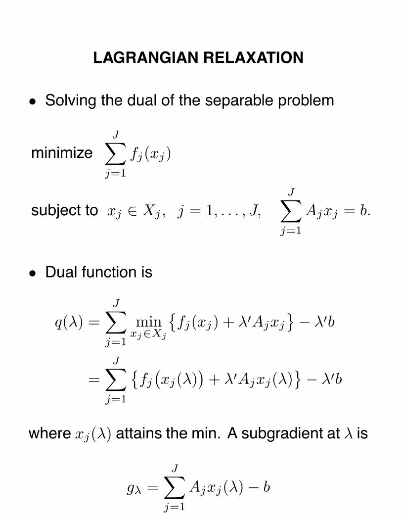
LAGRANGIAN RELAXATION
• Solving the dual of the separable problem
minimizeJ∑
j=1
fj(xj)
subject to xj ∈ Xj , j = 1, . . . , J,J∑
j=1
Ajxj = b.
• Dual function is
q(λ) =J∑
j=1
minxj∈Xj
{fj(xj) + λ′Ajxj
}− λ′b
=J∑
j=1
{fj
(xj(λ)
)+ λ′Ajxj(λ)
}− λ′b
where xj(λ) attains the min. A subgradient at λ is
gλ =J∑
j=1
Ajxj(λ) − b

DANTSIG-WOLFE DECOMPOSITION
• D-W decomposition method is just the cuttingplane applied to the dual problem maxλ q(λ).
• At the kth iteration, we solve the “approximatedual”
λk = arg maxλ∈�r
Qk(λ) ≡ mini=0,...,k−1
{q(λi)+(λ−λi)′gi
}
• Equivalent linear program in v and λ
maximize v
subject to v ≤ q(λi) + (λ − λi)′gi, i = 0, . . . , k − 1
The dual of this (called master problem) is
minimizek−1∑i=0
ξi(q(λi) − λi′gi
)
subject tok−1∑i=0
ξi = 1,k−1∑i=0
ξigi = 0,
ξi ≥ 0, i = 0, . . . , k − 1,

DANTSIG-WOLFE DECOMPOSITION (CONT.)
• The master problem is written as
minimizeJ∑
j=1
(k−1∑i=0
ξifj
(xj(λi)
))
subject tok−1∑i=0
ξi = 1,J∑
j=1
Aj
(k−1∑i=0
ξixj(λi)
)= b,
ξi ≥ 0, i = 0, . . . , k − 1.
• The primal cost function terms fj(xj) are ap-proximated by
k−1∑i=0
ξifj
(xj(λi)
)
• Vectors xj are expressed as
k−1∑i=0
ξixj(λi)

GEOMETRICAL INTERPRETATION
• Geometric interpretation of the master problem(the dual of the approximate dual solved in thecutting plane method) is inner linearization.
0
Xj
fj(xj)
xj
xj(λ0) xj(λ
1)xj(λ2) xj(λ
3)
• This is a “dual” operation to the one involvedin the cutting plane approximation, which can beviewed as outer linearization.