Embed Size (px)
Citation preview
Convex Functions Smooth Optimization Non-Smooth Optimization Stochastic Optimization
Convex OptimizationMark Schmidt - CMPT 419/726
Convex Functions Smooth Optimization Non-Smooth Optimization Stochastic Optimization
Motivation: Why Learn about Convex Optimization?
Why learn about optimization?
Optimization is at the core of many ML algorithms.
ML is driving a lot of modern research in optimization.
Why in particular learn about convex optimization?
Among only efficiently-solvable continuous problems.
You can do a lot with convex models.(least squares, lasso, generlized linear models, SVMs, CRFs)
Empirically effective non-convex methods are often basedmethods with good properties for convex objectives.
(functions are locally convex around minimizers)
Convex Functions Smooth Optimization Non-Smooth Optimization Stochastic Optimization
Outline
1 Convex Functions
2 Smooth Optimization
3 Non-Smooth Optimization
4 Stochastic Optimization
Convex Functions Smooth Optimization Non-Smooth Optimization Stochastic Optimization
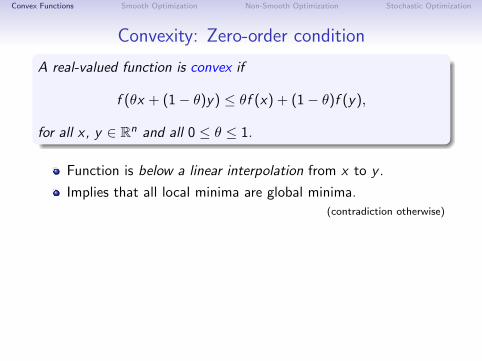
Convexity: Zero-order condition
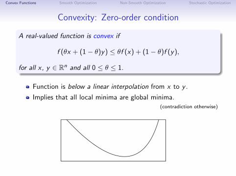
A real-valued function is convex if
f (θx + (1− θ)y) ≤ θf (x) + (1− θ)f (y),
for all x, y ∈ Rn and all 0 ≤ θ ≤ 1.
Function is below a linear interpolation from x to y .
Implies that all local minima are global minima.(contradiction otherwise)
Convex Functions Smooth Optimization Non-Smooth Optimization Stochastic Optimization
Convexity: Zero-order condition
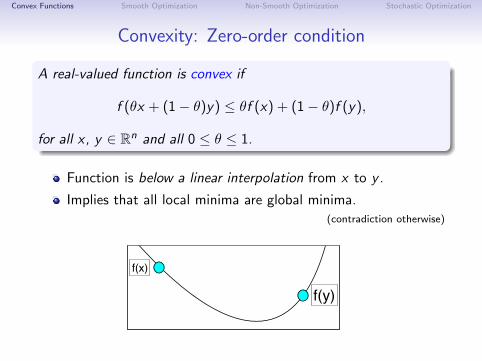
A real-valued function is convex if
f (θx + (1− θ)y) ≤ θf (x) + (1− θ)f (y),
for all x, y ∈ Rn and all 0 ≤ θ ≤ 1.
Function is below a linear interpolation from x to y .
Implies that all local minima are global minima.(contradiction otherwise)
f(x)
f(y)
Convex Functions Smooth Optimization Non-Smooth Optimization Stochastic Optimization
Convexity: Zero-order condition
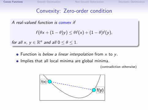
A real-valued function is convex if
f (θx + (1− θ)y) ≤ θf (x) + (1− θ)f (y),
for all x, y ∈ Rn and all 0 ≤ θ ≤ 1.
Function is below a linear interpolation from x to y .
Implies that all local minima are global minima.(contradiction otherwise)
f(x)
f(y)
0.5f(x) + 0.5f(y)
Convex Functions Smooth Optimization Non-Smooth Optimization Stochastic Optimization
Convexity: Zero-order condition
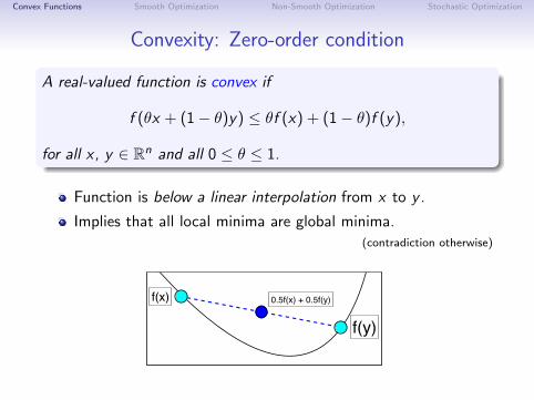
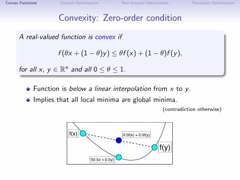
A real-valued function is convex if
f (θx + (1− θ)y) ≤ θf (x) + (1− θ)f (y),
for all x, y ∈ Rn and all 0 ≤ θ ≤ 1.
Function is below a linear interpolation from x to y .
Implies that all local minima are global minima.(contradiction otherwise)
f(x)
f(y)
0.5f(x) + 0.5f(y)
f(0.5x + 0.5y)
Convex Functions Smooth Optimization Non-Smooth Optimization Stochastic Optimization
Convexity: Zero-order condition
A real-valued function is convex if
f (θx + (1− θ)y) ≤ θf (x) + (1− θ)f (y),
for all x, y ∈ Rn and all 0 ≤ θ ≤ 1.
Function is below a linear interpolation from x to y .
Implies that all local minima are global minima.(contradiction otherwise)
Not convex
Convex Functions Smooth Optimization Non-Smooth Optimization Stochastic Optimization
Convexity: Zero-order condition
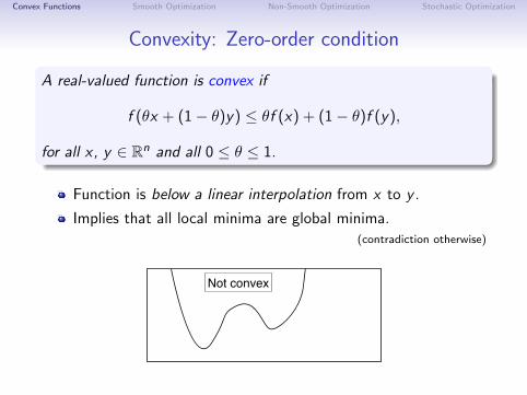
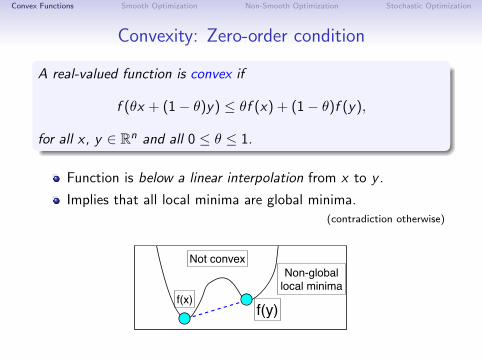
A real-valued function is convex if
f (θx + (1− θ)y) ≤ θf (x) + (1− θ)f (y),
for all x, y ∈ Rn and all 0 ≤ θ ≤ 1.
Function is below a linear interpolation from x to y .
Implies that all local minima are global minima.(contradiction otherwise)
f(x)f(y)
Not convexNon-global
local minima
Convex Functions Smooth Optimization Non-Smooth Optimization Stochastic Optimization
Convexity of Norms
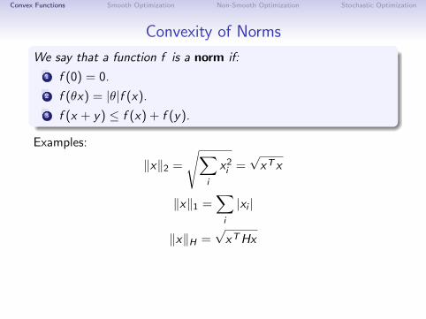
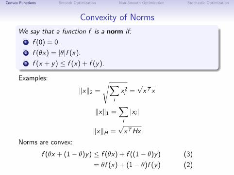
We say that a function f is a norm if:
1 f (0) = 0.
2 f (θx) = |θ|f (x).
3 f (x + y) ≤ f (x) + f (y).
Examples:
‖x‖2 =
√∑
i
x2i =√
xT x
‖x‖1 =∑
i
|xi |
‖x‖H =√
xTHx
Norms are convex:
f (θx + (1− θ)y) ≤ f (θx) + f ((1− θ)y) (3)
= θf (x) + (1− θ)f (y) (2)
Convex Functions Smooth Optimization Non-Smooth Optimization Stochastic Optimization
Convexity of Norms
We say that a function f is a norm if:
1 f (0) = 0.
2 f (θx) = |θ|f (x).
3 f (x + y) ≤ f (x) + f (y).
Examples:
‖x‖2 =
√∑
i
x2i =√
xT x
‖x‖1 =∑
i
|xi |
‖x‖H =√
xTHx
Norms are convex:
f (θx + (1− θ)y) ≤ f (θx) + f ((1− θ)y) (3)
= θf (x) + (1− θ)f (y) (2)
Convex Functions Smooth Optimization Non-Smooth Optimization Stochastic Optimization
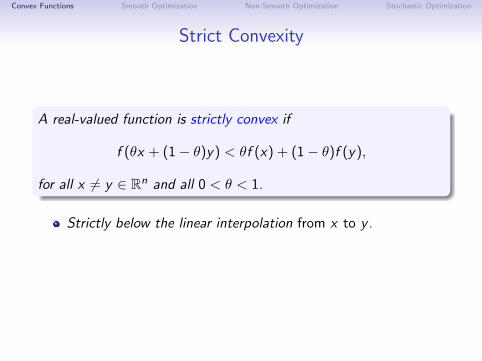
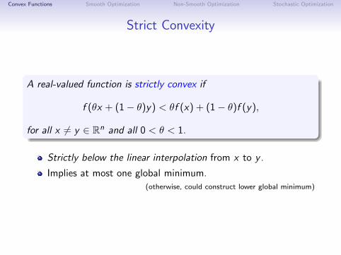
Strict Convexity
A real-valued function is strictly convex if
f (θx + (1− θ)y) < θf (x) + (1− θ)f (y),
for all x 6= y ∈ Rn and all 0 < θ < 1.
Strictly below the linear interpolation from x to y .
Implies at most one global minimum.(otherwise, could construct lower global minimum)
Convex Functions Smooth Optimization Non-Smooth Optimization Stochastic Optimization
Strict Convexity
A real-valued function is strictly convex if
f (θx + (1− θ)y) < θf (x) + (1− θ)f (y),
for all x 6= y ∈ Rn and all 0 < θ < 1.
Strictly below the linear interpolation from x to y .
Implies at most one global minimum.(otherwise, could construct lower global minimum)

Convex Functions Smooth Optimization Non-Smooth Optimization Stochastic Optimization
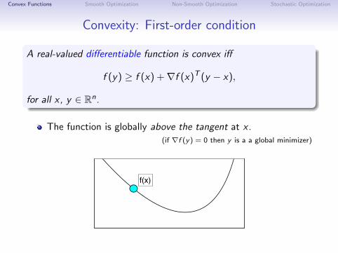
Convexity: First-order condition
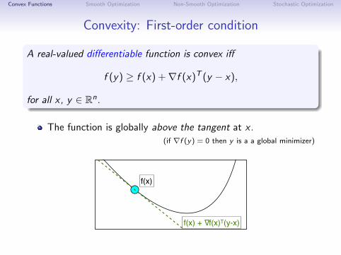
A real-valued differentiable function is convex iff
f (y) ≥ f (x) +∇f (x)T (y − x),
for all x, y ∈ Rn.
The function is globally above the tangent at x .(if ∇f (y) = 0 then y is a a global minimizer)
Convex Functions Smooth Optimization Non-Smooth Optimization Stochastic Optimization
Convexity: First-order condition
A real-valued differentiable function is convex iff
f (y) ≥ f (x) +∇f (x)T (y − x),
for all x, y ∈ Rn.
The function is globally above the tangent at x .(if ∇f (y) = 0 then y is a a global minimizer)
f(x)
f(x) + ∇f(x)T(y-x)
Convex Functions Smooth Optimization Non-Smooth Optimization Stochastic Optimization
Convexity: First-order condition
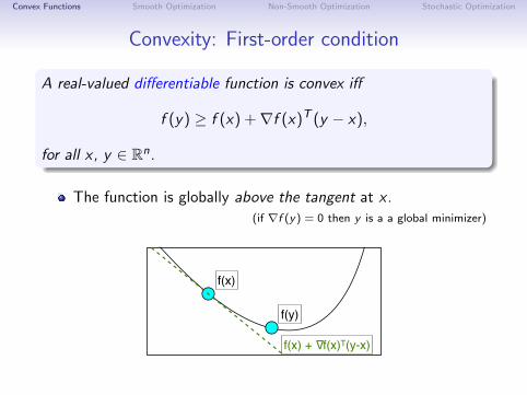
A real-valued differentiable function is convex iff
f (y) ≥ f (x) +∇f (x)T (y − x),
for all x, y ∈ Rn.
The function is globally above the tangent at x .(if ∇f (y) = 0 then y is a a global minimizer)
f(x)
f(x) + ∇f(x)T(y-x)
f(y)
Convex Functions Smooth Optimization Non-Smooth Optimization Stochastic Optimization
Convexity: Second-order condition
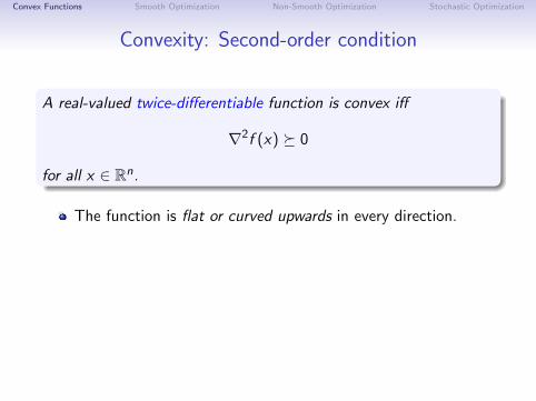
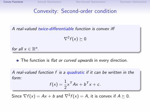
A real-valued twice-differentiable function is convex iff
∇2f (x) 0
for all x ∈ Rn.
The function is flat or curved upwards in every direction.
A real-valued function f is a quadratic if it can be written in theform:
f (x) =1
2xTAx + bT x + c .
Since ∇f (x) = Ax + b and ∇2f (x) = A, it is convex if A 0.
Convex Functions Smooth Optimization Non-Smooth Optimization Stochastic Optimization
Convexity: Second-order condition
A real-valued twice-differentiable function is convex iff
∇2f (x) 0
for all x ∈ Rn.
The function is flat or curved upwards in every direction.
A real-valued function f is a quadratic if it can be written in theform:
f (x) =1
2xTAx + bT x + c .
Since ∇f (x) = Ax + b and ∇2f (x) = A, it is convex if A 0.
Convex Functions Smooth Optimization Non-Smooth Optimization Stochastic Optimization
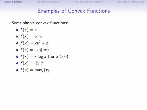
Examples of Convex Functions
Some simple convex functions:
f (x) = c
f (x) = aT x
f (x) = xa2 + b
f (x) = exp(ax)
f (x) = x log x (for x > 0)
f (x) = ||x ||2f (x) = maxixi
Some other notable examples:
f (x , y) = log(ex + ey )
f (X ) = log det X (for X positive-definite).
f (x ,Y ) = xTY−1x (for Y positive-definite)
Convex Functions Smooth Optimization Non-Smooth Optimization Stochastic Optimization
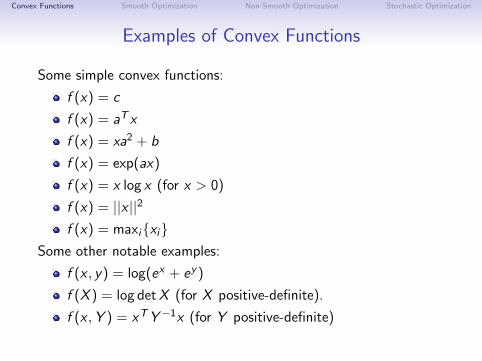
Examples of Convex Functions
Some simple convex functions:
f (x) = c
f (x) = aT x
f (x) = xa2 + b
f (x) = exp(ax)
f (x) = x log x (for x > 0)
f (x) = ||x ||2f (x) = maxixi
Some other notable examples:
f (x , y) = log(ex + ey )
f (X ) = log det X (for X positive-definite).
f (x ,Y ) = xTY−1x (for Y positive-definite)
Convex Functions Smooth Optimization Non-Smooth Optimization Stochastic Optimization
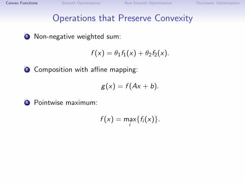
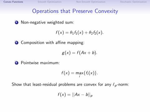
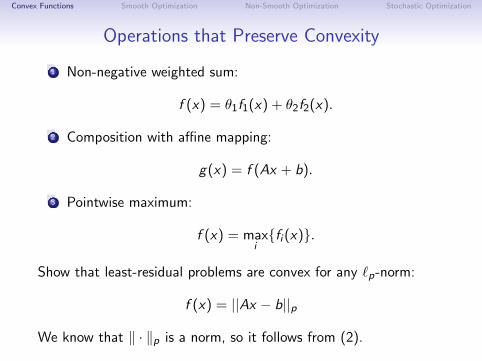
Operations that Preserve Convexity
1 Non-negative weighted sum:
f (x) = θ1f1(x) + θ2f2(x).
2 Composition with affine mapping:
g(x) = f (Ax + b).
3 Pointwise maximum:
f (x) = maxifi (x).
Show that least-residual problems are convex for any `p-norm:
f (x) = ||Ax − b||p
We know that ‖ · ‖p is a norm, so it follows from (2).
Convex Functions Smooth Optimization Non-Smooth Optimization Stochastic Optimization
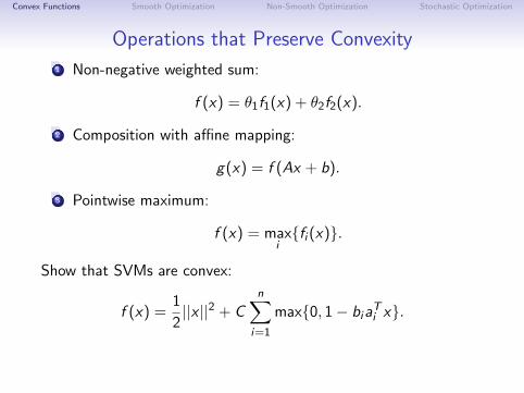
Operations that Preserve Convexity
1 Non-negative weighted sum:
f (x) = θ1f1(x) + θ2f2(x).
2 Composition with affine mapping:
g(x) = f (Ax + b).
3 Pointwise maximum:
f (x) = maxifi (x).
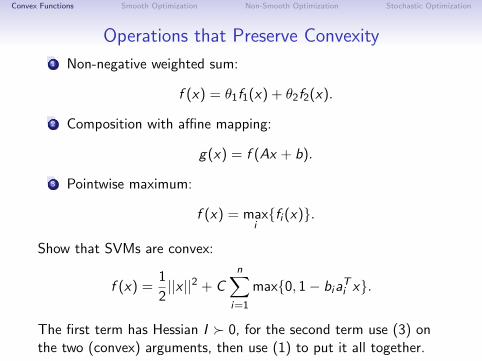
Show that SVMs are convex:
f (x) =1
2||x ||2 + C
n∑
i=1
max0, 1− biaTi x.
The first term has Hessian I 0, for the second term use (3) onthe two (convex) arguments, then use (1) to put it all together.
Convex Functions Smooth Optimization Non-Smooth Optimization Stochastic Optimization
Operations that Preserve Convexity
1 Non-negative weighted sum:
f (x) = θ1f1(x) + θ2f2(x).
2 Composition with affine mapping:
g(x) = f (Ax + b).
3 Pointwise maximum:
f (x) = maxifi (x).
Show that SVMs are convex:
f (x) =1
2||x ||2 + C
n∑
i=1
max0, 1− biaTi x.
The first term has Hessian I 0, for the second term use (3) onthe two (convex) arguments, then use (1) to put it all together.
Convex Functions Smooth Optimization Non-Smooth Optimization Stochastic Optimization
Outline
1 Convex Functions
2 Smooth Optimization
3 Non-Smooth Optimization
4 Stochastic Optimization
Convex Functions Smooth Optimization Non-Smooth Optimization Stochastic Optimization
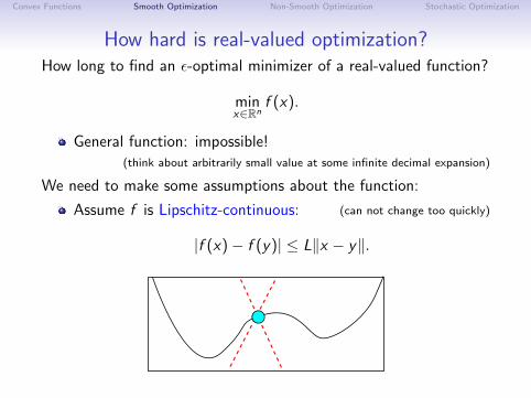
How hard is real-valued optimization?How long to find an ε-optimal minimizer of a real-valued function?
minx∈Rn
f (x).
General function: impossible!(think about arbitrarily small value at some infinite decimal expansion)
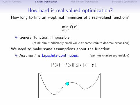
We need to make some assumptions about the function:
Assume f is Lipschitz-continuous: (can not change too quickly)
|f (x)− f (y)| ≤ L‖x − y‖.
Convex Functions Smooth Optimization Non-Smooth Optimization Stochastic Optimization
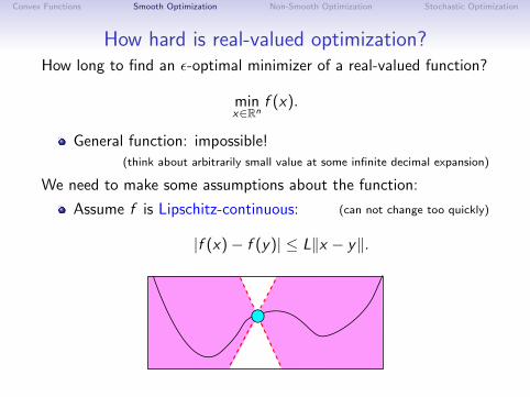
How hard is real-valued optimization?How long to find an ε-optimal minimizer of a real-valued function?
minx∈Rn
f (x).
General function: impossible!(think about arbitrarily small value at some infinite decimal expansion)
We need to make some assumptions about the function:
Assume f is Lipschitz-continuous: (can not change too quickly)
|f (x)− f (y)| ≤ L‖x − y‖.
Convex Functions Smooth Optimization Non-Smooth Optimization Stochastic Optimization
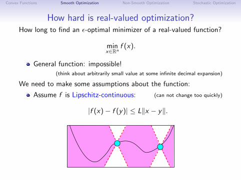
How hard is real-valued optimization?How long to find an ε-optimal minimizer of a real-valued function?
minx∈Rn
f (x).
General function: impossible!(think about arbitrarily small value at some infinite decimal expansion)
We need to make some assumptions about the function:
Assume f is Lipschitz-continuous: (can not change too quickly)
|f (x)− f (y)| ≤ L‖x − y‖.
Convex Functions Smooth Optimization Non-Smooth Optimization Stochastic Optimization
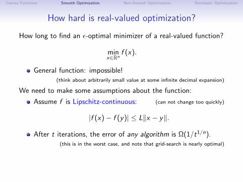
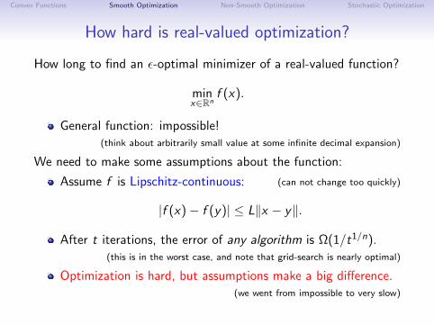
How hard is real-valued optimization?
How long to find an ε-optimal minimizer of a real-valued function?
minx∈Rn
f (x).
General function: impossible!(think about arbitrarily small value at some infinite decimal expansion)
We need to make some assumptions about the function:
Assume f is Lipschitz-continuous: (can not change too quickly)
|f (x)− f (y)| ≤ L‖x − y‖.
After t iterations, the error of any algorithm is Ω(1/t1/n).(this is in the worst case, and note that grid-search is nearly optimal)
Optimization is hard, but assumptions make a big difference.(we went from impossible to very slow)
Convex Functions Smooth Optimization Non-Smooth Optimization Stochastic Optimization
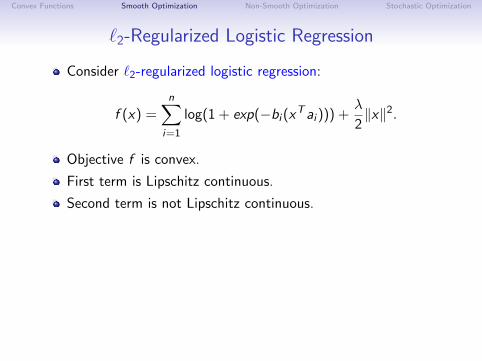
`2-Regularized Logistic Regression
Consider `2-regularized logistic regression:
f (x) =n∑
i=1
log(1 + exp(−bi (xTai ))) +λ
2‖x‖2.
Objective f is convex.
First term is Lipschitz continuous.
Second term is not Lipschitz continuous.
But we haveµI ∇2f (x) LI .
(L = 14‖A‖2
2 + λ, µ = λ)
Gradient is Lipschitz-continuous.
Function is strongly-convex.(implies strict convexity, and existence of unique solution)
Convex Functions Smooth Optimization Non-Smooth Optimization Stochastic Optimization
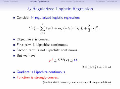
`2-Regularized Logistic Regression
Consider `2-regularized logistic regression:
f (x) =n∑
i=1
log(1 + exp(−bi (xTai ))) +λ
2‖x‖2.
Objective f is convex.
First term is Lipschitz continuous.
Second term is not Lipschitz continuous.
But we haveµI ∇2f (x) LI .
(L = 14‖A‖2
2 + λ, µ = λ)
Gradient is Lipschitz-continuous.
Function is strongly-convex.(implies strict convexity, and existence of unique solution)
Convex Functions Smooth Optimization Non-Smooth Optimization Stochastic Optimization
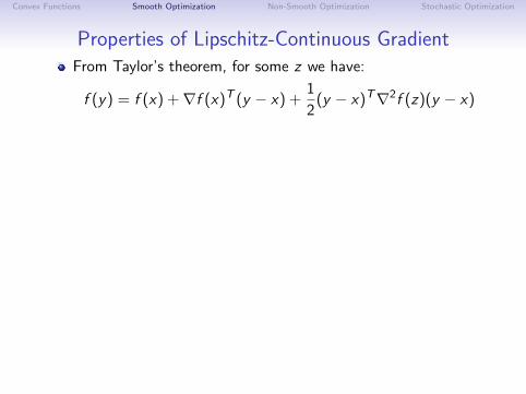
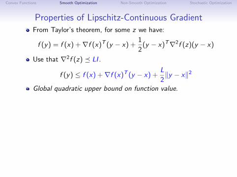
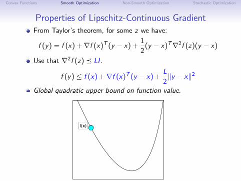
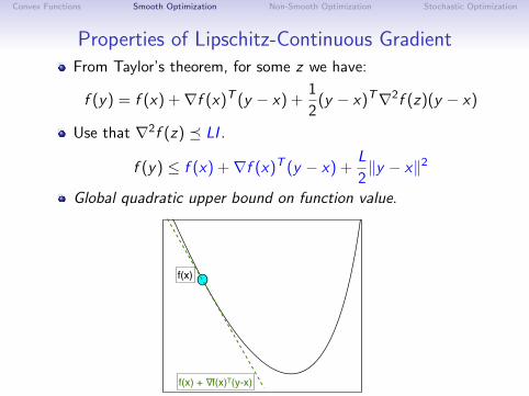
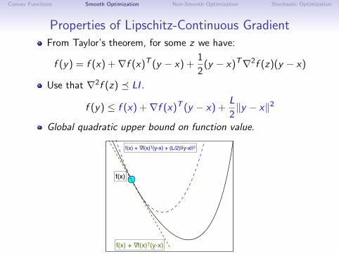
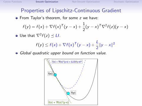
Properties of Lipschitz-Continuous GradientFrom Taylor’s theorem, for some z we have:
f (y) = f (x) +∇f (x)T (y − x) +1
2(y − x)T∇2f (z)(y − x)
Use that ∇2f (z) LI .
f (y) ≤ f (x) +∇f (x)T (y − x) +L
2‖y − x‖2
Global quadratic upper bound on function value.
Convex Functions Smooth Optimization Non-Smooth Optimization Stochastic Optimization
Properties of Lipschitz-Continuous GradientFrom Taylor’s theorem, for some z we have:
f (y) = f (x) +∇f (x)T (y − x) +1
2(y − x)T∇2f (z)(y − x)
Use that ∇2f (z) LI .
f (y) ≤ f (x) +∇f (x)T (y − x) +L
2‖y − x‖2
Global quadratic upper bound on function value.
f(x)
f(x) + ∇f(x)T(y-x)
f(x) + ∇f(x)T(y-x) + (L/2)||y-x||2
Convex Functions Smooth Optimization Non-Smooth Optimization Stochastic Optimization
Properties of Lipschitz-Continuous GradientFrom Taylor’s theorem, for some z we have:
f (y) = f (x) +∇f (x)T (y − x) +1
2(y − x)T∇2f (z)(y − x)
Use that ∇2f (z) LI .
f (y) ≤ f (x) +∇f (x)T (y − x) +L
2‖y − x‖2
Global quadratic upper bound on function value.
f(x)
f(x) + ∇f(x)T(y-x)
f(y)
f(x) + ∇f(x)T(y-x) + (L/2)||y-x||2

Convex Functions Smooth Optimization Non-Smooth Optimization Stochastic Optimization
Properties of Lipschitz-Continuous GradientFrom Taylor’s theorem, for some z we have:
f (y) = f (x) +∇f (x)T (y − x) +1
2(y − x)T∇2f (z)(y − x)
Use that ∇2f (z) LI .
f (y) ≤ f (x) +∇f (x)T (y − x) +L
2‖y − x‖2
Global quadratic upper bound on function value.
Stochastic vs. deterministic methods
• Minimizing g(!) =1
n
n!
i=1
fi(!) with fi(!) = ""yi, !
!!(xi)#
+ µ"(!)
• Batch gradient descent: !t = !t"1!#tg#(!t"1) = !t"1!
#t
n
n!
i=1
f #i(!t"1)
• Stochastic gradient descent: !t = !t"1 ! #tf#i(t)(!t"1)
Convex Functions Smooth Optimization Non-Smooth Optimization Stochastic Optimization
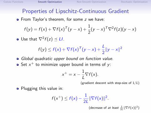
Properties of Lipschitz-Continuous Gradient
From Taylor’s theorem, for some z we have:
f (y) = f (x) +∇f (x)T (y − x) +1
2(y − x)T∇2f (z)(y − x)
Use that ∇2f (z) LI .
f (y) ≤ f (x) +∇f (x)T (y − x) +L
2‖y − x‖2
Global quadratic upper bound on function value.
Set x+ to minimize upper bound in terms of y :
x+ = x − 1
L∇f (x).
(gradient descent with step-size of 1/L)
Plugging this value in:
f (x+) ≤ f (x)− 1
2L‖∇f (x)‖2.
(decrease of at least 12L‖∇f (x)‖2)
Convex Functions Smooth Optimization Non-Smooth Optimization Stochastic Optimization
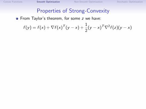
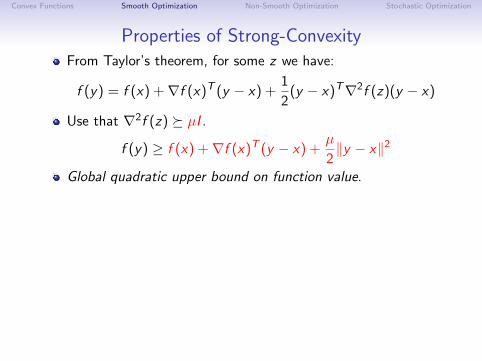
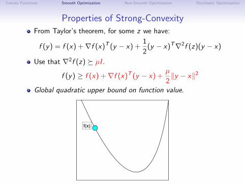
Properties of Strong-ConvexityFrom Taylor’s theorem, for some z we have:
f (y) = f (x) +∇f (x)T (y − x) +1
2(y − x)T∇2f (z)(y − x)
Use that ∇2f (z) µI .
f (y) ≥ f (x) +∇f (x)T (y − x) +µ
2‖y − x‖2
Global quadratic upper bound on function value.
Convex Functions Smooth Optimization Non-Smooth Optimization Stochastic Optimization
Properties of Strong-ConvexityFrom Taylor’s theorem, for some z we have:
f (y) = f (x) +∇f (x)T (y − x) +1
2(y − x)T∇2f (z)(y − x)
Use that ∇2f (z) µI .
f (y) ≥ f (x) +∇f (x)T (y − x) +µ
2‖y − x‖2
Global quadratic upper bound on function value.
f(x)
f(x) + ∇f(x)T(y-x)
Convex Functions Smooth Optimization Non-Smooth Optimization Stochastic Optimization
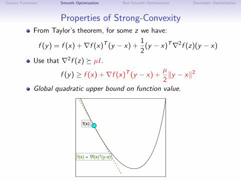
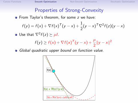
Properties of Strong-ConvexityFrom Taylor’s theorem, for some z we have:
f (y) = f (x) +∇f (x)T (y − x) +1
2(y − x)T∇2f (z)(y − x)
Use that ∇2f (z) µI .
f (y) ≥ f (x) +∇f (x)T (y − x) +µ
2‖y − x‖2
Global quadratic upper bound on function value.
f(x)
f(x) + ∇f(x)T(y-x)
f(x) + ∇f(x)T(y-x) + (μ/2)||y-x||2
Convex Functions Smooth Optimization Non-Smooth Optimization Stochastic Optimization
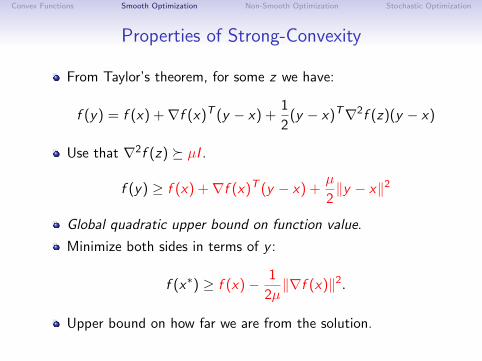
Properties of Strong-Convexity
From Taylor’s theorem, for some z we have:
f (y) = f (x) +∇f (x)T (y − x) +1
2(y − x)T∇2f (z)(y − x)
Use that ∇2f (z) µI .
f (y) ≥ f (x) +∇f (x)T (y − x) +µ
2‖y − x‖2
Global quadratic upper bound on function value.
Minimize both sides in terms of y :
f (x∗) ≥ f (x)− 1
2µ‖∇f (x)‖2.
Upper bound on how far we are from the solution.
Convex Functions Smooth Optimization Non-Smooth Optimization Stochastic Optimization
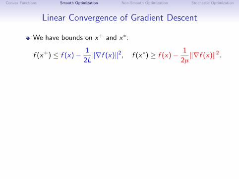
Linear Convergence of Gradient Descent
We have bounds on x+ and x∗:
f (x+) ≤ f (x)− 1
2L‖∇f (x)‖2, f (x∗) ≥ f (x)− 1
2µ‖∇f (x)‖2.
Convex Functions Smooth Optimization Non-Smooth Optimization Stochastic Optimization
Linear Convergence of Gradient Descent
We have bounds on x+ and x∗:
f (x+) ≤ f (x)− 1
2L‖∇f (x)‖2, f (x∗) ≥ f (x)− 1
2µ‖∇f (x)‖2.
f(x)
Convex Functions Smooth Optimization Non-Smooth Optimization Stochastic Optimization
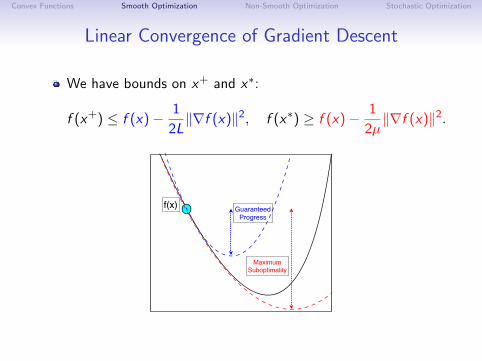
Linear Convergence of Gradient Descent
We have bounds on x+ and x∗:
f (x+) ≤ f (x)− 1
2L‖∇f (x)‖2, f (x∗) ≥ f (x)− 1
2µ‖∇f (x)‖2.
f(x) GuaranteedProgress
Convex Functions Smooth Optimization Non-Smooth Optimization Stochastic Optimization
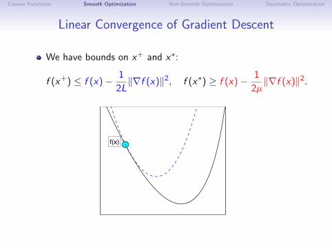
Linear Convergence of Gradient Descent
We have bounds on x+ and x∗:
f (x+) ≤ f (x)− 1
2L‖∇f (x)‖2, f (x∗) ≥ f (x)− 1
2µ‖∇f (x)‖2.
f(x) GuaranteedProgress
Convex Functions Smooth Optimization Non-Smooth Optimization Stochastic Optimization
Linear Convergence of Gradient Descent
We have bounds on x+ and x∗:
f (x+) ≤ f (x)− 1
2L‖∇f (x)‖2, f (x∗) ≥ f (x)− 1
2µ‖∇f (x)‖2.
f(x) GuaranteedProgress
MaximumSuboptimality
Convex Functions Smooth Optimization Non-Smooth Optimization Stochastic Optimization
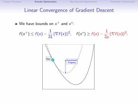
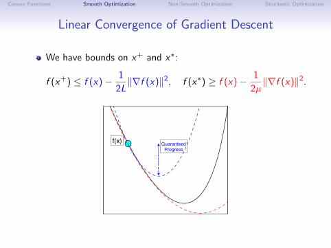
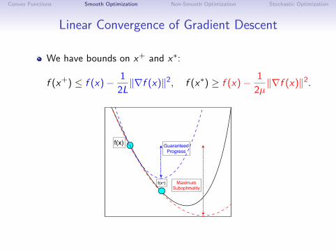
Linear Convergence of Gradient Descent
We have bounds on x+ and x∗:
f (x+) ≤ f (x)− 1
2L‖∇f (x)‖2, f (x∗) ≥ f (x)− 1
2µ‖∇f (x)‖2.
f(x) GuaranteedProgress
MaximumSuboptimality
f(x+)
Convex Functions Smooth Optimization Non-Smooth Optimization Stochastic Optimization
Linear Convergence of Gradient Descent
We have bounds on x+ and x∗:
f (x+) ≤ f (x)− 1
2L‖∇f (x)‖2, f (x∗) ≥ f (x)− 1
2µ‖∇f (x)‖2.
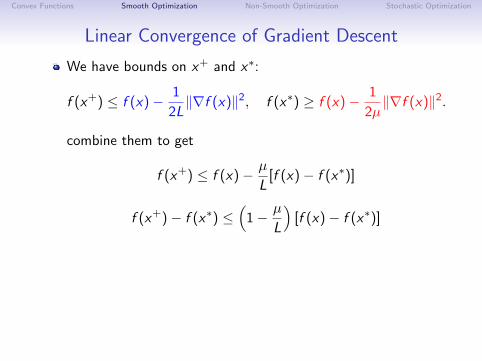
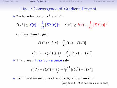
combine them to get
f (x+) ≤ f (x)− µ
L[f (x)− f (x∗)]
f (x+)− f (x∗) ≤(
1− µ
L
)[f (x)− f (x∗)]
This gives a linear convergence rate:
f (x t)− f (x∗) ≤(
1− µ
L
)t[f (x0)− f (x∗)]
Each iteration multiplies the error by a fixed amount.(very fast if µ/L is not too close to one)
Convex Functions Smooth Optimization Non-Smooth Optimization Stochastic Optimization
Linear Convergence of Gradient Descent
We have bounds on x+ and x∗:
f (x+) ≤ f (x)− 1
2L‖∇f (x)‖2, f (x∗) ≥ f (x)− 1
2µ‖∇f (x)‖2.
combine them to get
f (x+) ≤ f (x)− µ
L[f (x)− f (x∗)]
f (x+)− f (x∗) ≤(
1− µ
L
)[f (x)− f (x∗)]
This gives a linear convergence rate:
f (x t)− f (x∗) ≤(
1− µ
L
)t[f (x0)− f (x∗)]
Each iteration multiplies the error by a fixed amount.(very fast if µ/L is not too close to one)
Convex Functions Smooth Optimization Non-Smooth Optimization Stochastic Optimization
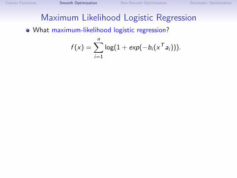
Maximum Likelihood Logistic RegressionWhat maximum-likelihood logistic regression?
f (x) =n∑
i=1
log(1 + exp(−bi (xTai ))).
We now only have
0 ∇2f (x) LI .
Convexity only gives a linear upper bound on f (x∗):
f (x∗) ≤ f (x) +∇f (x)T (x∗ − x)
Convex Functions Smooth Optimization Non-Smooth Optimization Stochastic Optimization
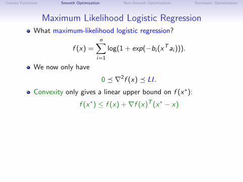
Maximum Likelihood Logistic RegressionWhat maximum-likelihood logistic regression?
f (x) =n∑
i=1
log(1 + exp(−bi (xTai ))).
We now only have
0 ∇2f (x) LI .
Convexity only gives a linear upper bound on f (x∗):
f (x∗) ≤ f (x) +∇f (x)T (x∗ − x)

Convex Functions Smooth Optimization Non-Smooth Optimization Stochastic Optimization
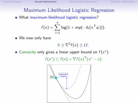
Maximum Likelihood Logistic RegressionWhat maximum-likelihood logistic regression?
f (x) =n∑
i=1
log(1 + exp(−bi (xTai ))).
We now only have
0 ∇2f (x) LI .
Convexity only gives a linear upper bound on f (x∗):
f (x∗) ≤ f (x) +∇f (x)T (x∗ − x)
f(x)GuaranteedProgress
Convex Functions Smooth Optimization Non-Smooth Optimization Stochastic Optimization
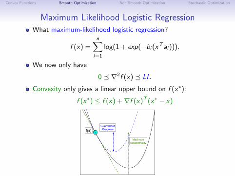
Maximum Likelihood Logistic RegressionWhat maximum-likelihood logistic regression?
f (x) =n∑
i=1
log(1 + exp(−bi (xTai ))).
We now only have
0 ∇2f (x) LI .
Convexity only gives a linear upper bound on f (x∗):
f (x∗) ≤ f (x) +∇f (x)T (x∗ − x)
f(x)GuaranteedProgress
MaximumSuboptimality
Convex Functions Smooth Optimization Non-Smooth Optimization Stochastic Optimization
Maximum Likelihood Logistic Regression
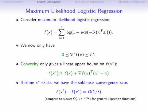
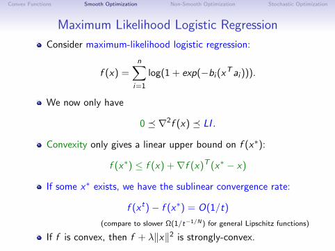
Consider maximum-likelihood logistic regression:
f (x) =n∑
i=1
log(1 + exp(−bi (xTai ))).
We now only have
0 ∇2f (x) LI .
Convexity only gives a linear upper bound on f (x∗):
f (x∗) ≤ f (x) +∇f (x)T (x∗ − x)
If some x∗ exists, we have the sublinear convergence rate:
f (x t)− f (x∗) = O(1/t)
(compare to slower Ω(1/t−1/N) for general Lipschitz functions)
If f is convex, then f + λ‖x‖2 is strongly-convex.
Convex Functions Smooth Optimization Non-Smooth Optimization Stochastic Optimization
Maximum Likelihood Logistic Regression
Consider maximum-likelihood logistic regression:
f (x) =n∑
i=1
log(1 + exp(−bi (xTai ))).
We now only have
0 ∇2f (x) LI .
Convexity only gives a linear upper bound on f (x∗):
f (x∗) ≤ f (x) +∇f (x)T (x∗ − x)
If some x∗ exists, we have the sublinear convergence rate:
f (x t)− f (x∗) = O(1/t)
(compare to slower Ω(1/t−1/N) for general Lipschitz functions)
If f is convex, then f + λ‖x‖2 is strongly-convex.
Convex Functions Smooth Optimization Non-Smooth Optimization Stochastic Optimization
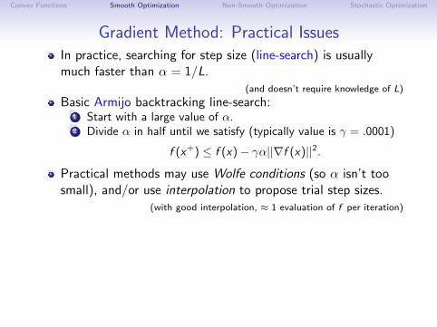
Gradient Method: Practical IssuesIn practice, searching for step size (line-search) is usuallymuch faster than α = 1/L.
(and doesn’t require knowledge of L)
Basic Armijo backtracking line-search:1 Start with a large value of α.2 Divide α in half until we satisfy (typically value is γ = .0001)
f (x+) ≤ f (x)− γα||∇f (x)||2.Practical methods may use Wolfe conditions (so α isn’t toosmall), and/or use interpolation to propose trial step sizes.
(with good interpolation, ≈ 1 evaluation of f per iteration)
Also, check your derivative code!
∇i f (x) ≈ f (x + δei )− f (x)
δFor large-scale problems you can check a random direction d :
∇f (x)Td ≈ f (x + δd)− f (x)
δ
Convex Functions Smooth Optimization Non-Smooth Optimization Stochastic Optimization
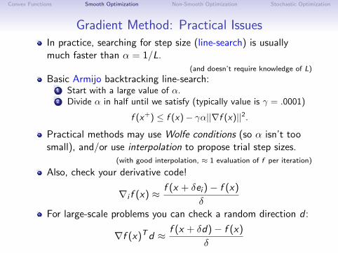
Gradient Method: Practical IssuesIn practice, searching for step size (line-search) is usuallymuch faster than α = 1/L.
(and doesn’t require knowledge of L)
Basic Armijo backtracking line-search:1 Start with a large value of α.2 Divide α in half until we satisfy (typically value is γ = .0001)
f (x+) ≤ f (x)− γα||∇f (x)||2.
Practical methods may use Wolfe conditions (so α isn’t toosmall), and/or use interpolation to propose trial step sizes.
(with good interpolation, ≈ 1 evaluation of f per iteration)
Also, check your derivative code!
∇i f (x) ≈ f (x + δei )− f (x)
δFor large-scale problems you can check a random direction d :
∇f (x)Td ≈ f (x + δd)− f (x)
δ
Convex Functions Smooth Optimization Non-Smooth Optimization Stochastic Optimization
Gradient Method: Practical IssuesIn practice, searching for step size (line-search) is usuallymuch faster than α = 1/L.
(and doesn’t require knowledge of L)
Basic Armijo backtracking line-search:1 Start with a large value of α.2 Divide α in half until we satisfy (typically value is γ = .0001)
f (x+) ≤ f (x)− γα||∇f (x)||2.Practical methods may use Wolfe conditions (so α isn’t toosmall), and/or use interpolation to propose trial step sizes.
(with good interpolation, ≈ 1 evaluation of f per iteration)
Also, check your derivative code!
∇i f (x) ≈ f (x + δei )− f (x)
δFor large-scale problems you can check a random direction d :
∇f (x)Td ≈ f (x + δd)− f (x)
δ
Convex Functions Smooth Optimization Non-Smooth Optimization Stochastic Optimization
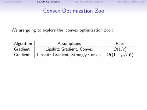
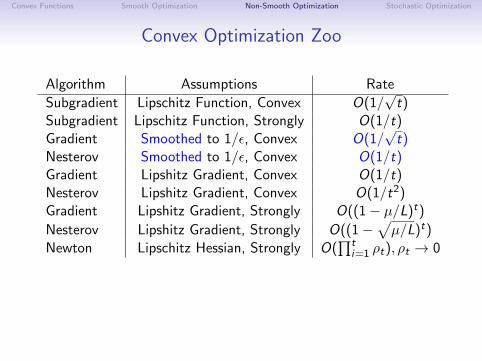
Convex Optimization Zoo
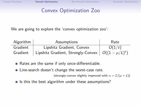
We are going to explore the ‘convex optimization zoo’:
Algorithm Assumptions Rate
Gradient Lipshitz Gradient, Convex O(1/t)Gradient Lipshitz Gradient, Strongly-Convex O((1− µ/L)t)
Rates are the same if only once-differentiable.
Line-search doesn’t change the worst-case rate.(strongly-convex slightly improved with α = 2/(µ+ L))
Is this the best algorithm under these assumptions?
Convex Functions Smooth Optimization Non-Smooth Optimization Stochastic Optimization
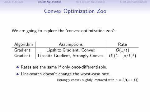
Convex Optimization Zoo
We are going to explore the ‘convex optimization zoo’:
Algorithm Assumptions Rate
Gradient Lipshitz Gradient, Convex O(1/t)Gradient Lipshitz Gradient, Strongly-Convex O((1− µ/L)t)
Rates are the same if only once-differentiable.
Line-search doesn’t change the worst-case rate.(strongly-convex slightly improved with α = 2/(µ+ L))
Is this the best algorithm under these assumptions?
Convex Functions Smooth Optimization Non-Smooth Optimization Stochastic Optimization
Accelerated Gradient Method
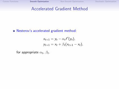
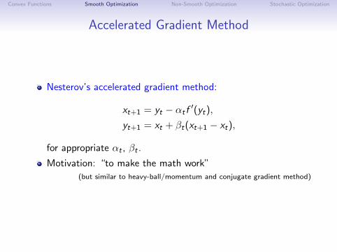
Nesterov’s accelerated gradient method:
xt+1 = yt − αt f′(yt),
yt+1 = xt + βt(xt+1 − xt),
for appropriate αt , βt .
Motivation: “to make the math work”(but similar to heavy-ball/momentum and conjugate gradient method)
Convex Functions Smooth Optimization Non-Smooth Optimization Stochastic Optimization
Accelerated Gradient Method
Nesterov’s accelerated gradient method:
xt+1 = yt − αt f′(yt),
yt+1 = xt + βt(xt+1 − xt),
for appropriate αt , βt .
Motivation: “to make the math work”(but similar to heavy-ball/momentum and conjugate gradient method)
Convex Functions Smooth Optimization Non-Smooth Optimization Stochastic Optimization
Convex Optimization Zoo
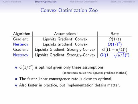
Algorithm Assumptions Rate
Gradient Lipshitz Gradient, Convex O(1/t)Nesterov Lipshitz Gradient, Convex O(1/t2)Gradient Lipshitz Gradient, Strongly-Convex O((1− µ/L)t)
Nesterov Lipshitz Gradient, Strongly-Convex O((1−√µ/L)t)
O(1/t2) is optimal given only these assumptions.(sometimes called the optimal gradient method)
The faster linear convergence rate is close to optimal.
Also faster in practice, but implementation details matter.

Convex Functions Smooth Optimization Non-Smooth Optimization Stochastic Optimization
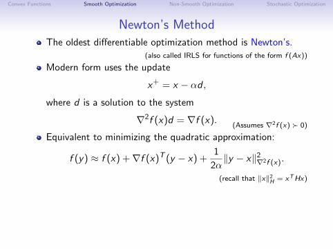
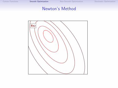
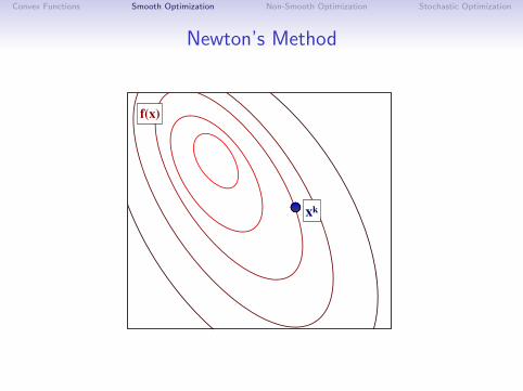
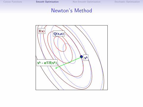
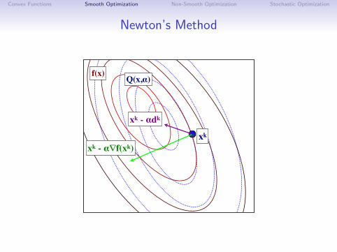
Newton’s Method
The oldest differentiable optimization method is Newton’s.(also called IRLS for functions of the form f (Ax))
Modern form uses the update
x+ = x − αd ,
where d is a solution to the system
∇2f (x)d = ∇f (x).(Assumes ∇2f (x) 0)
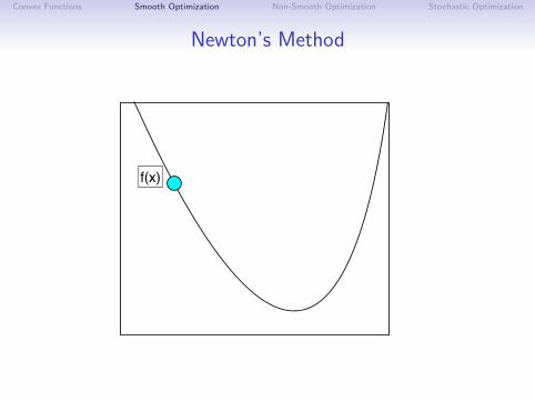
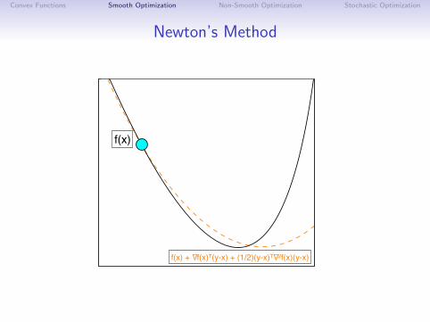
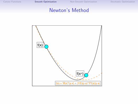
Equivalent to minimizing the quadratic approximation:
f (y) ≈ f (x) +∇f (x)T (y − x) +1
2α‖y − x‖2
∇2f (x).
(recall that ‖x‖2H = xTHx)
We can generalize the Armijo condition to
f (x+) ≤ f (x) + γα∇f ′(x)Td .
Has a natural step length of α = 1.(always accepted when close to a minimizer)
Convex Functions Smooth Optimization Non-Smooth Optimization Stochastic Optimization
Newton’s Method
The oldest differentiable optimization method is Newton’s.(also called IRLS for functions of the form f (Ax))
Modern form uses the update
x+ = x − αd ,
where d is a solution to the system
∇2f (x)d = ∇f (x).(Assumes ∇2f (x) 0)
Equivalent to minimizing the quadratic approximation:
f (y) ≈ f (x) +∇f (x)T (y − x) +1
2α‖y − x‖2
∇2f (x).
(recall that ‖x‖2H = xTHx)
We can generalize the Armijo condition to
f (x+) ≤ f (x) + γα∇f ′(x)Td .
Has a natural step length of α = 1.(always accepted when close to a minimizer)
Convex Functions Smooth Optimization Non-Smooth Optimization Stochastic Optimization
Newton’s Method
f(x)
Convex Functions Smooth Optimization Non-Smooth Optimization Stochastic Optimization
Newton’s Method
f(x)
f(x) + ∇f(x)T(y-x) + (1/2)(y-x)T∇2f(x)(y-x)
Convex Functions Smooth Optimization Non-Smooth Optimization Stochastic Optimization
Newton’s Method
f(x)
f(x+)
f(x) + ∇f(x)T(y-x) + (1/2)(y-x)T∇2f(x)(y-x)
Convex Functions Smooth Optimization Non-Smooth Optimization Stochastic Optimization
Newton’s Method
f(x)
Convex Functions Smooth Optimization Non-Smooth Optimization Stochastic Optimization
Newton’s Method
f(x)
xk

Convex Functions Smooth Optimization Non-Smooth Optimization Stochastic Optimization
Newton’s Method
f(x)
xk
xk - !!f(xk)
Convex Functions Smooth Optimization Non-Smooth Optimization Stochastic Optimization
Newton’s Method
f(x)
xk
xk - !!f(xk)
Q(x,!)
Convex Functions Smooth Optimization Non-Smooth Optimization Stochastic Optimization
Newton’s Method
f(x)
xk
xk - !!f(xk)
Q(x,!)
xk - !dk
Convex Functions Smooth Optimization Non-Smooth Optimization Stochastic Optimization
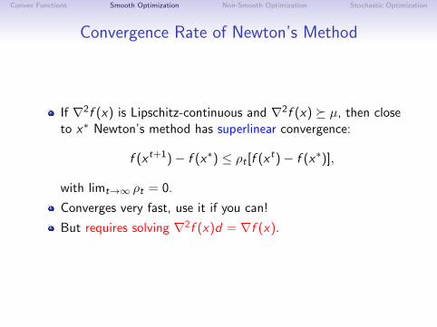
Convergence Rate of Newton’s Method
If ∇2f (x) is Lipschitz-continuous and ∇2f (x) µ, then closeto x∗ Newton’s method has superlinear convergence:
f (x t+1)− f (x∗) ≤ ρt [f (x t)− f (x∗)],
with limt→∞ ρt = 0.
Converges very fast, use it if you can!
But requires solving ∇2f (x)d = ∇f (x).
Convex Functions Smooth Optimization Non-Smooth Optimization Stochastic Optimization
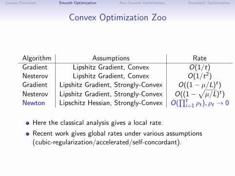
Convex Optimization Zoo
Algorithm Assumptions Rate
Gradient Lipshitz Gradient, Convex O(1/t)Nesterov Lipshitz Gradient, Convex O(1/t2)Gradient Lipshitz Gradient, Strongly-Convex O((1− µ/L)t)
Nesterov Lipshitz Gradient, Strongly-Convex O((1−√µ/L)t)
Newton Lipschitz Hessian, Strongly-Convex O(∏t
i=1 ρt), ρt → 0
Here the classical analysis gives a local rate.
Recent work gives global rates under various assumptions(cubic-regularization/accelerated/self-concordant).
Convex Functions Smooth Optimization Non-Smooth Optimization Stochastic Optimization
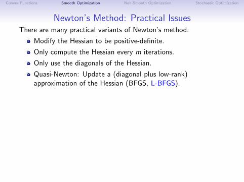
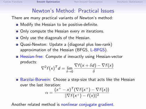
Newton’s Method: Practical IssuesThere are many practical variants of Newton’s method:
Modify the Hessian to be positive-definite.
Only compute the Hessian every m iterations.
Only use the diagonals of the Hessian.
Quasi-Newton: Update a (diagonal plus low-rank)approximation of the Hessian (BFGS, L-BFGS).
Hessian-free: Compute d inexactly using Hessian-vectorproducts:
∇2f (x)Td = limδ→0
∇f (x + δd)−∇f (x)
δ
Barzilai-Borwein: Choose a step-size that acts like the Hessianover the last iteration:
α =(x+ − x)T (∇f (x+)−∇f (x))
‖∇f (x+)− f (x)‖2
Another related method is nonlinear conjugate gradient.
Convex Functions Smooth Optimization Non-Smooth Optimization Stochastic Optimization
Outline
1 Convex Functions
2 Smooth Optimization
3 Non-Smooth Optimization
4 Stochastic Optimization
Convex Functions Smooth Optimization Non-Smooth Optimization Stochastic Optimization
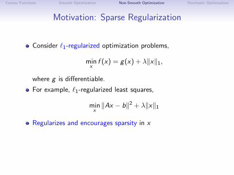
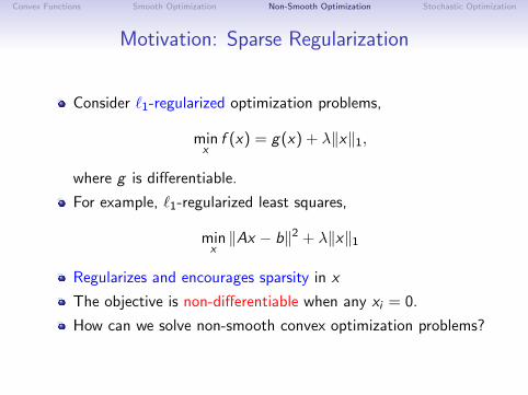
Motivation: Sparse Regularization
Consider `1-regularized optimization problems,
minx
f (x) = g(x) + λ‖x‖1,
where g is differentiable.
For example, `1-regularized least squares,
minx‖Ax − b‖2 + λ‖x‖1
Regularizes and encourages sparsity in x
The objective is non-differentiable when any xi = 0.
How can we solve non-smooth convex optimization problems?
Convex Functions Smooth Optimization Non-Smooth Optimization Stochastic Optimization
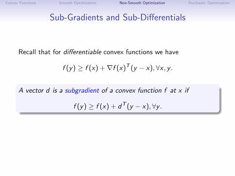
Sub-Gradients and Sub-Differentials
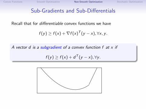
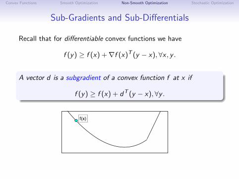
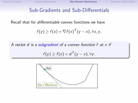
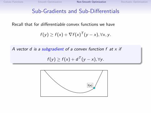
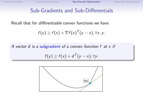
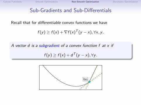
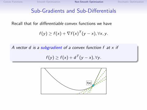
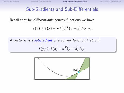
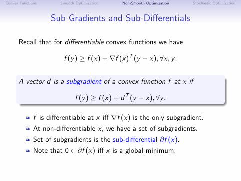
Recall that for differentiable convex functions we have
f (y) ≥ f (x) +∇f (x)T (y − x), ∀x , y .
A vector d is a subgradient of a convex function f at x if
f (y) ≥ f (x) + dT (y − x),∀y .
Convex Functions Smooth Optimization Non-Smooth Optimization Stochastic Optimization
Sub-Gradients and Sub-Differentials
Recall that for differentiable convex functions we have
f (y) ≥ f (x) +∇f (x)T (y − x), ∀x , y .
A vector d is a subgradient of a convex function f at x if
f (y) ≥ f (x) + dT (y − x),∀y .
f(x)
f(x) + ∇f(x)T(y-x)
Convex Functions Smooth Optimization Non-Smooth Optimization Stochastic Optimization
Sub-Gradients and Sub-Differentials
Recall that for differentiable convex functions we have
f (y) ≥ f (x) +∇f (x)T (y − x), ∀x , y .
A vector d is a subgradient of a convex function f at x if
f (y) ≥ f (x) + dT (y − x),∀y .
f(x)
Convex Functions Smooth Optimization Non-Smooth Optimization Stochastic Optimization
Sub-Gradients and Sub-Differentials
Recall that for differentiable convex functions we have
f (y) ≥ f (x) +∇f (x)T (y − x), ∀x , y .
A vector d is a subgradient of a convex function f at x if
f (y) ≥ f (x) + dT (y − x),∀y .
f is differentiable at x iff ∇f (x) is the only subgradient.
At non-differentiable x , we have a set of subgradients.
Set of subgradients is the sub-differential ∂f (x).
Note that 0 ∈ ∂f (x) iff x is a global minimum.
Convex Functions Smooth Optimization Non-Smooth Optimization Stochastic Optimization
Sub-Differential of Absolute Value and Max Functions
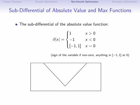
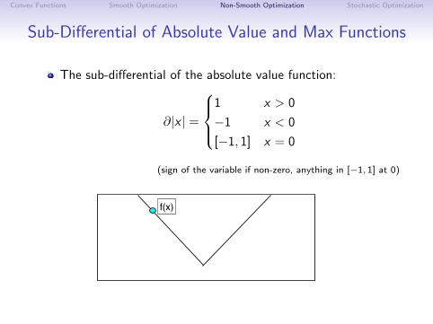
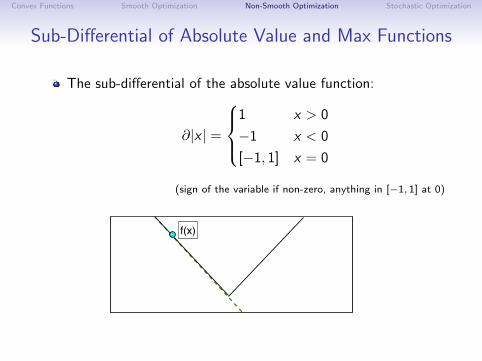
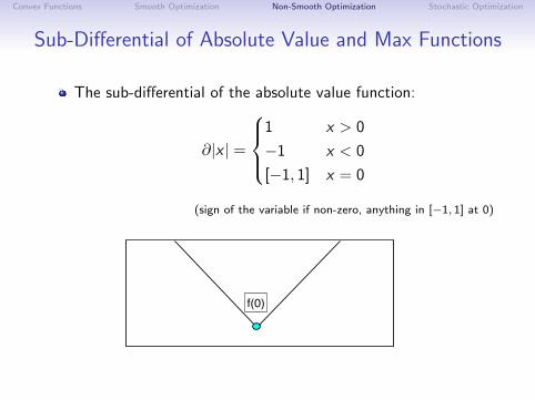
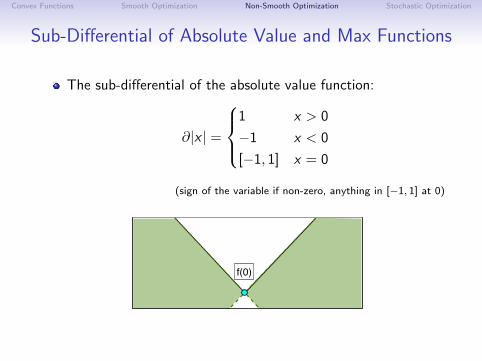
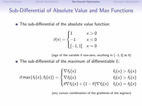
The sub-differential of the absolute value function:
∂|x | =
1 x > 0
−1 x < 0
[−1, 1] x = 0
(sign of the variable if non-zero, anything in [−1, 1] at 0)
Convex Functions Smooth Optimization Non-Smooth Optimization Stochastic Optimization
Sub-Differential of Absolute Value and Max Functions
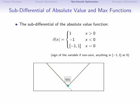
The sub-differential of the absolute value function:
∂|x | =
1 x > 0
−1 x < 0
[−1, 1] x = 0
(sign of the variable if non-zero, anything in [−1, 1] at 0)
f(x)
Convex Functions Smooth Optimization Non-Smooth Optimization Stochastic Optimization
Sub-Differential of Absolute Value and Max Functions
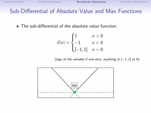
The sub-differential of the absolute value function:
∂|x | =
1 x > 0
−1 x < 0
[−1, 1] x = 0
(sign of the variable if non-zero, anything in [−1, 1] at 0)
f(x)
Convex Functions Smooth Optimization Non-Smooth Optimization Stochastic Optimization
Sub-Differential of Absolute Value and Max Functions
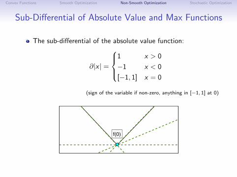
The sub-differential of the absolute value function:
∂|x | =
1 x > 0
−1 x < 0
[−1, 1] x = 0
(sign of the variable if non-zero, anything in [−1, 1] at 0)
f(0)
Convex Functions Smooth Optimization Non-Smooth Optimization Stochastic Optimization
Sub-Differential of Absolute Value and Max Functions
The sub-differential of the absolute value function:
∂|x | =
1 x > 0
−1 x < 0
[−1, 1] x = 0
(sign of the variable if non-zero, anything in [−1, 1] at 0)
f(0)

Convex Functions Smooth Optimization Non-Smooth Optimization Stochastic Optimization
Sub-Differential of Absolute Value and Max Functions
The sub-differential of the absolute value function:
∂|x | =
1 x > 0
−1 x < 0
[−1, 1] x = 0
(sign of the variable if non-zero, anything in [−1, 1] at 0)
f(0)
Convex Functions Smooth Optimization Non-Smooth Optimization Stochastic Optimization
Sub-Differential of Absolute Value and Max Functions
The sub-differential of the absolute value function:
∂|x | =
1 x > 0
−1 x < 0
[−1, 1] x = 0
(sign of the variable if non-zero, anything in [−1, 1] at 0)
f(0)
Convex Functions Smooth Optimization Non-Smooth Optimization Stochastic Optimization
Sub-Differential of Absolute Value and Max Functions
The sub-differential of the absolute value function:
∂|x | =
1 x > 0
−1 x < 0
[−1, 1] x = 0
(sign of the variable if non-zero, anything in [−1, 1] at 0)
f(0)
Convex Functions Smooth Optimization Non-Smooth Optimization Stochastic Optimization
Sub-Differential of Absolute Value and Max Functions
The sub-differential of the absolute value function:
∂|x | =
1 x > 0
−1 x < 0
[−1, 1] x = 0
(sign of the variable if non-zero, anything in [−1, 1] at 0)
f(0)
Convex Functions Smooth Optimization Non-Smooth Optimization Stochastic Optimization
Sub-Differential of Absolute Value and Max Functions
The sub-differential of the absolute value function:
∂|x | =
1 x > 0
−1 x < 0
[−1, 1] x = 0
(sign of the variable if non-zero, anything in [−1, 1] at 0)
The sub-differential of the maximum of differentiable fi :
∂maxf1(x), f2(x) =
∇f1(x) f1(x) > f2(x)
∇f2(x) f2(x) > f1(x)
θ∇f1(x) + (1− θ)∇f2(x) f1(x) = f2(x)
(any convex combination of the gradients of the argmax)
Convex Functions Smooth Optimization Non-Smooth Optimization Stochastic Optimization
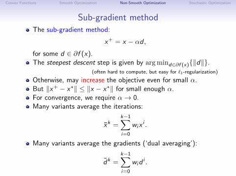
Sub-gradient methodThe sub-gradient method:
x+ = x − αd ,
for some d ∈ ∂f (x).
The steepest descent step is given by argmind∈∂f (x)‖d‖.(often hard to compute, but easy for `1-regularization)
Otherwise, may increase the objective even for small α.But ‖x+ − x∗‖ ≤ ‖x − x∗‖ for small enough α.For convergence, we require α→ 0.Many variants average the iterations:
xk =k−1∑
i=0
wixi .
Many variants average the gradients (‘dual averaging’):
dk =k−1∑
i=0
widi .
Convex Functions Smooth Optimization Non-Smooth Optimization Stochastic Optimization
Sub-gradient methodThe sub-gradient method:
x+ = x − αd ,
for some d ∈ ∂f (x).The steepest descent step is given by argmind∈∂f (x)‖d‖.
(often hard to compute, but easy for `1-regularization)
Otherwise, may increase the objective even for small α.But ‖x+ − x∗‖ ≤ ‖x − x∗‖ for small enough α.For convergence, we require α→ 0.
Many variants average the iterations:
xk =k−1∑
i=0
wixi .
Many variants average the gradients (‘dual averaging’):
dk =k−1∑
i=0
widi .
Convex Functions Smooth Optimization Non-Smooth Optimization Stochastic Optimization
Sub-gradient methodThe sub-gradient method:
x+ = x − αd ,
for some d ∈ ∂f (x).The steepest descent step is given by argmind∈∂f (x)‖d‖.
(often hard to compute, but easy for `1-regularization)
Otherwise, may increase the objective even for small α.But ‖x+ − x∗‖ ≤ ‖x − x∗‖ for small enough α.For convergence, we require α→ 0.Many variants average the iterations:
xk =k−1∑
i=0
wixi .
Many variants average the gradients (‘dual averaging’):
dk =k−1∑
i=0
widi .
Convex Functions Smooth Optimization Non-Smooth Optimization Stochastic Optimization
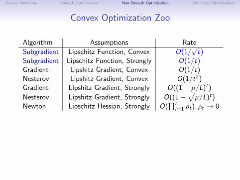
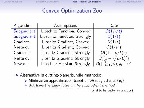
Convex Optimization Zoo
Algorithm Assumptions Rate
Subgradient Lipschitz Function, Convex O(1/√
t)Subgradient Lipschitz Function, Strongly O(1/t)Gradient Lipshitz Gradient, Convex O(1/t)Nesterov Lipshitz Gradient, Convex O(1/t2)Gradient Lipshitz Gradient, Strongly O((1− µ/L)t)
Nesterov Lipshitz Gradient, Strongly O((1−√µ/L)t)
Newton Lipschitz Hessian, Strongly O(∏t
i=1 ρt), ρt → 0
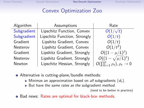
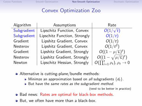
Alternative is cutting-plane/bundle methods:Minimze an approximation based on all subgradients dt.But have the same rates as the subgradient method.
(tend to be better in practice)
Bad news: Rates are optimal for black-box methods.
But, we often have more than a black-box.
Convex Functions Smooth Optimization Non-Smooth Optimization Stochastic Optimization
Convex Optimization Zoo
Algorithm Assumptions Rate
Subgradient Lipschitz Function, Convex O(1/√
t)Subgradient Lipschitz Function, Strongly O(1/t)Gradient Lipshitz Gradient, Convex O(1/t)Nesterov Lipshitz Gradient, Convex O(1/t2)Gradient Lipshitz Gradient, Strongly O((1− µ/L)t)
Nesterov Lipshitz Gradient, Strongly O((1−√µ/L)t)
Newton Lipschitz Hessian, Strongly O(∏t
i=1 ρt), ρt → 0
Alternative is cutting-plane/bundle methods:Minimze an approximation based on all subgradients dt.But have the same rates as the subgradient method.
(tend to be better in practice)
Bad news: Rates are optimal for black-box methods.
But, we often have more than a black-box.
Convex Functions Smooth Optimization Non-Smooth Optimization Stochastic Optimization
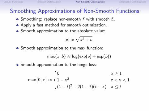
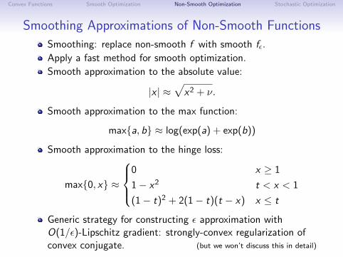
Smoothing Approximations of Non-Smooth Functions
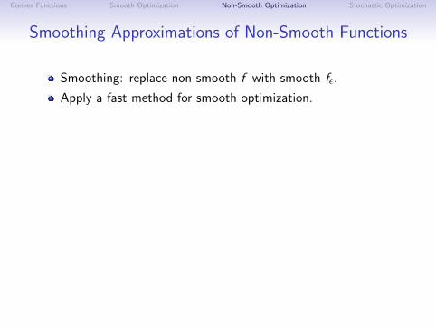
Smoothing: replace non-smooth f with smooth fε.
Apply a fast method for smooth optimization.
Smooth approximation to the absolute value:
|x | ≈√
x2 + ν.
Convex Functions Smooth Optimization Non-Smooth Optimization Stochastic Optimization
Smoothing Approximations of Non-Smooth Functions
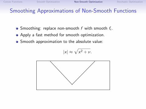
Smoothing: replace non-smooth f with smooth fε.
Apply a fast method for smooth optimization.
Smooth approximation to the absolute value:
|x | ≈√
x2 + ν.
Convex Functions Smooth Optimization Non-Smooth Optimization Stochastic Optimization
Smoothing Approximations of Non-Smooth Functions
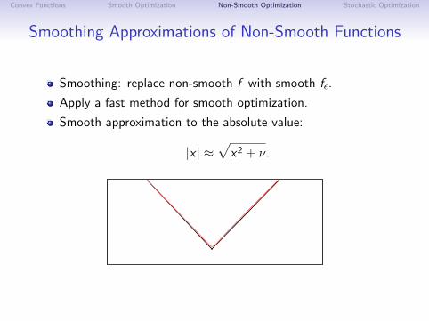
Smoothing: replace non-smooth f with smooth fε.
Apply a fast method for smooth optimization.
Smooth approximation to the absolute value:
|x | ≈√
x2 + ν.
Convex Functions Smooth Optimization Non-Smooth Optimization Stochastic Optimization
Smoothing Approximations of Non-Smooth Functions
Smoothing: replace non-smooth f with smooth fε.
Apply a fast method for smooth optimization.
Smooth approximation to the absolute value:
|x | ≈√
x2 + ν.
Smooth approximation to the max function:
maxa, b ≈ log(exp(a) + exp(b))
Smooth approximation to the hinge loss:
max0, x ≈
0 x ≥ 1
1− x2 t < x < 1
(1− t)2 + 2(1− t)(t − x) x ≤ t
Generic strategy for constructing ε approximation withO(1/ε)-Lipschitz gradient: strongly-convex regularization ofconvex conjugate. (but we won’t discuss this in detail)
Convex Functions Smooth Optimization Non-Smooth Optimization Stochastic Optimization
Convex Optimization Zoo
Algorithm Assumptions Rate
Subgradient Lipschitz Function, Convex O(1/√
t)Subgradient Lipschitz Function, Strongly O(1/t)Gradient Smoothed to 1/ε, Convex O(1/
√t)
Nesterov Smoothed to 1/ε, Convex O(1/t)Gradient Lipshitz Gradient, Convex O(1/t)Nesterov Lipshitz Gradient, Convex O(1/t2)Gradient Lipshitz Gradient, Strongly O((1− µ/L)t)
Nesterov Lipshitz Gradient, Strongly O((1−√µ/L)t)
Newton Lipschitz Hessian, Strongly O(∏t
i=1 ρt), ρt → 0
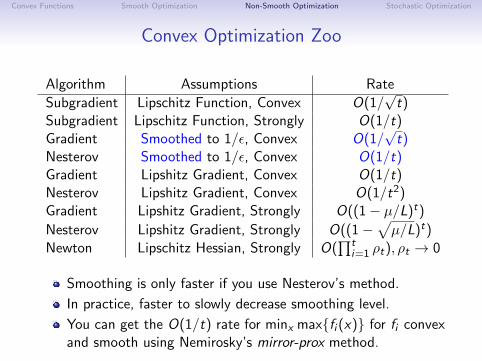
Smoothing is only faster if you use Nesterov’s method.
In practice, faster to slowly decrease smoothing level.
You can get the O(1/t) rate for minx maxfi (x) for fi convexand smooth using Nemirosky’s mirror-prox method.
Convex Functions Smooth Optimization Non-Smooth Optimization Stochastic Optimization
Convex Optimization Zoo
Algorithm Assumptions Rate
Subgradient Lipschitz Function, Convex O(1/√
t)Subgradient Lipschitz Function, Strongly O(1/t)Gradient Smoothed to 1/ε, Convex O(1/
√t)
Nesterov Smoothed to 1/ε, Convex O(1/t)Gradient Lipshitz Gradient, Convex O(1/t)Nesterov Lipshitz Gradient, Convex O(1/t2)Gradient Lipshitz Gradient, Strongly O((1− µ/L)t)
Nesterov Lipshitz Gradient, Strongly O((1−√µ/L)t)
Newton Lipschitz Hessian, Strongly O(∏t
i=1 ρt), ρt → 0
Smoothing is only faster if you use Nesterov’s method.
In practice, faster to slowly decrease smoothing level.
You can get the O(1/t) rate for minx maxfi (x) for fi convexand smooth using Nemirosky’s mirror-prox method.
Convex Functions Smooth Optimization Non-Smooth Optimization Stochastic Optimization
Converting to Constrained Optimization
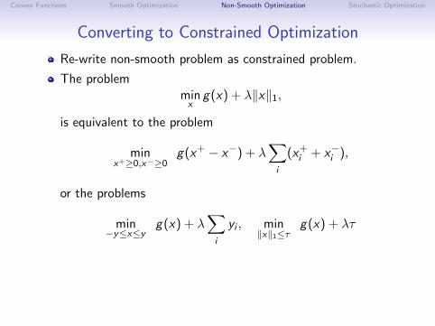
Re-write non-smooth problem as constrained problem.
The problemminx
g(x) + λ‖x‖1,
is equivalent to the problem
minx+≥0,x−≥0
g(x+ − x−) + λ∑
i
(x+i + x−i ),
or the problems
min−y≤x≤y
g(x) + λ∑
i
yi , min‖x‖1≤τ
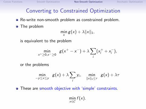
g(x) + λτ
These are smooth objective with ‘simple’ constraints.
minx∈C
f (x).
Convex Functions Smooth Optimization Non-Smooth Optimization Stochastic Optimization
Converting to Constrained Optimization
Re-write non-smooth problem as constrained problem.
The problemminx
g(x) + λ‖x‖1,
is equivalent to the problem
minx+≥0,x−≥0
g(x+ − x−) + λ∑
i
(x+i + x−i ),
or the problems
min−y≤x≤y
g(x) + λ∑
i
yi , min‖x‖1≤τ
g(x) + λτ
These are smooth objective with ‘simple’ constraints.
minx∈C
f (x).
Convex Functions Smooth Optimization Non-Smooth Optimization Stochastic Optimization
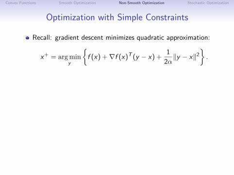
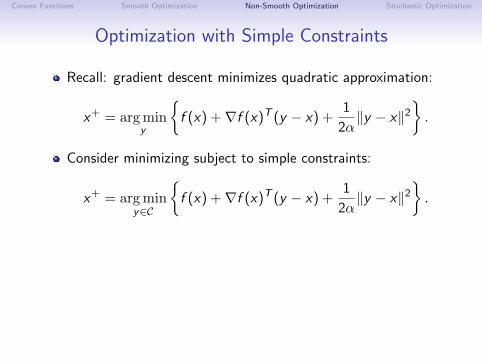
Optimization with Simple Constraints
Recall: gradient descent minimizes quadratic approximation:
x+ = argminy
f (x) +∇f (x)T (y − x) +
1
2α‖y − x‖2
.
Consider minimizing subject to simple constraints:
x+ = argminy∈C
f (x) +∇f (x)T (y − x) +
1
2α‖y − x‖2
.
Equivalent to projection of gradient descent:
xGD = x − α∇f (x),
x+ = argminy∈C
‖y − xGD‖
,
Convex Functions Smooth Optimization Non-Smooth Optimization Stochastic Optimization
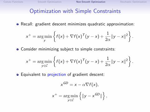
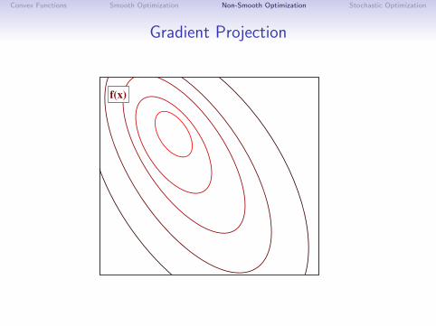
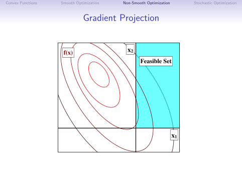
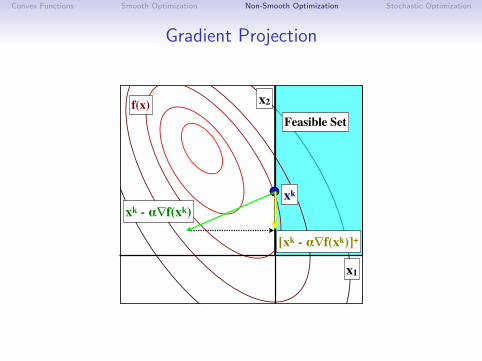
Gradient Projection
f(x)
Convex Functions Smooth Optimization Non-Smooth Optimization Stochastic Optimization
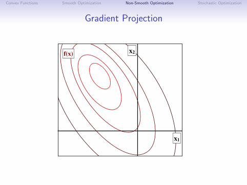
Gradient Projection
f(x)
x1
x2
Convex Functions Smooth Optimization Non-Smooth Optimization Stochastic Optimization
Gradient Projection
f(x)Feasible Set
x1
x2
Convex Functions Smooth Optimization Non-Smooth Optimization Stochastic Optimization
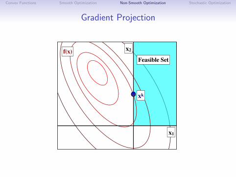
Gradient Projection
f(x)Feasible Set
xk
x1
x2
Convex Functions Smooth Optimization Non-Smooth Optimization Stochastic Optimization
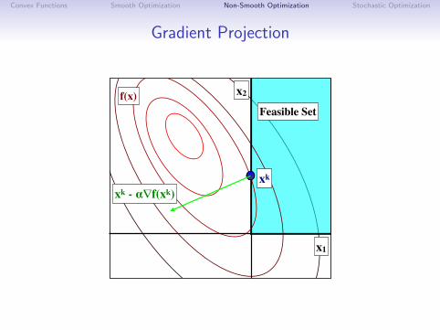
Gradient Projection
f(x)Feasible Set
xk
x1
x2
xk - !!f(xk)
Convex Functions Smooth Optimization Non-Smooth Optimization Stochastic Optimization
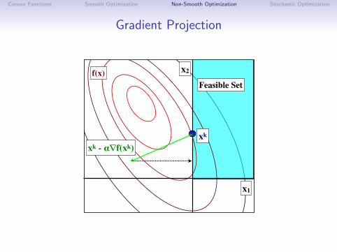
Gradient Projection
f(x)Feasible Set
xk
x1
x2
xk - !!f(xk)
Convex Functions Smooth Optimization Non-Smooth Optimization Stochastic Optimization
Gradient Projection
f(x)Feasible Set
[xk - !!f(xk)]+
xk
x1
x2
xk - !!f(xk)

Convex Functions Smooth Optimization Non-Smooth Optimization Stochastic Optimization
Projection Onto Simple Sets
Projections onto simple sets:
argminy≥0 ‖y − x‖ = maxx , 0argminl≤y≤u ‖y − x‖ = maxl ,minx , uargminaT y=b ‖y − x‖ = x + (b − aT x)a/‖a‖2.
argminaT y≥b ‖y − x‖ =
x aT x ≥ b
x + (b − aT x)a/‖a‖2 aT x < b
argmin‖y‖≤τ ‖y − x‖ = τx/‖x‖.Linear-time algorithm for `1-norm ‖y‖1 ≤ τ .
Linear-time algorithm for probability simplex y ≥ 0,∑
y = 1.
Intersection of simple sets: Dykstra’s algorithm.
Convex Functions Smooth Optimization Non-Smooth Optimization Stochastic Optimization
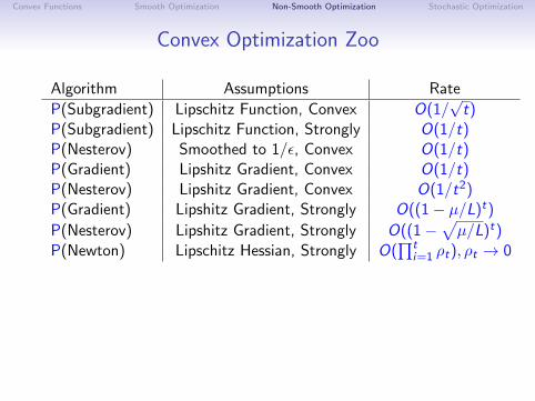
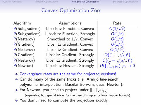
Convex Optimization Zoo
Algorithm Assumptions Rate
P(Subgradient) Lipschitz Function, Convex O(1/√
t)P(Subgradient) Lipschitz Function, Strongly O(1/t)P(Nesterov) Smoothed to 1/ε, Convex O(1/t)P(Gradient) Lipshitz Gradient, Convex O(1/t)P(Nesterov) Lipshitz Gradient, Convex O(1/t2)P(Gradient) Lipshitz Gradient, Strongly O((1− µ/L)t)
P(Nesterov) Lipshitz Gradient, Strongly O((1−√µ/L)t)
P(Newton) Lipschitz Hessian, Strongly O(∏t
i=1 ρt), ρt → 0
Convergence rates are the same for projected versions!Can do many of the same tricks (i.e. Armijo line-search,polynomial interpolation, Barzilai-Borwein, quasi-Newton).For Newton, you need to project under ‖ · ‖∇2f (x)
(expensive, but special tricks for the case of simplex or lower/upper bounds)
You don’t need to compute the projection exactly.
Convex Functions Smooth Optimization Non-Smooth Optimization Stochastic Optimization
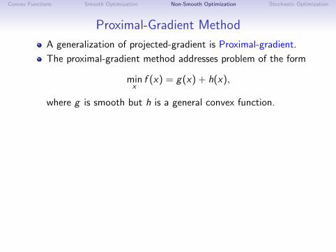
Proximal-Gradient Method
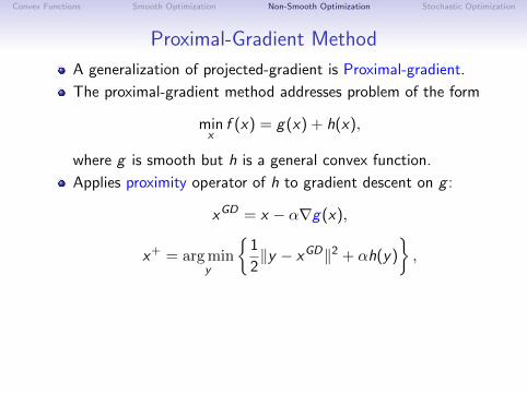
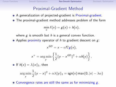
A generalization of projected-gradient is Proximal-gradient.
The proximal-gradient method addresses problem of the form
minx
f (x) = g(x) + h(x),
where g is smooth but h is a general convex function.
Applies proximity operator of h to gradient descent on g :
xGD = x − α∇g(x),
x+ = argminy
1
2‖y − xGD‖2 + αh(y)
,
If h(x) = λ‖x‖1, then
argminy
1
2‖y − x‖2 + αλ‖y‖1 = sgn(x) max0, |x | − λα
Convergence rates are still the same as for minimizing g .
Convex Functions Smooth Optimization Non-Smooth Optimization Stochastic Optimization
Proximal-Gradient Method
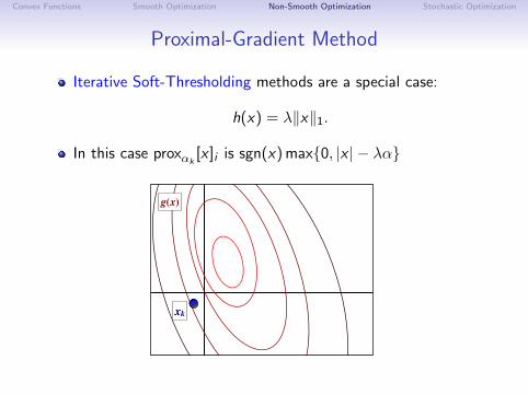
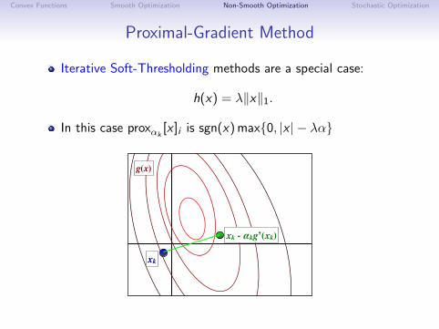
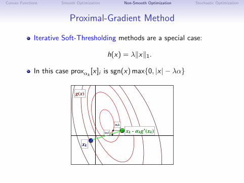
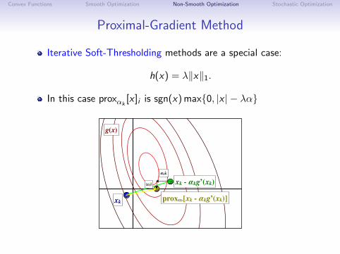
Iterative Soft-Thresholding methods are a special case:
h(x) = λ‖x‖1.
In this case proxαk[x ]i is sgn(x) max0, |x | − λα
g(x)
xk
Convex Functions Smooth Optimization Non-Smooth Optimization Stochastic Optimization
Proximal-Gradient Method
Iterative Soft-Thresholding methods are a special case:
h(x) = λ‖x‖1.
In this case proxαk[x ]i is sgn(x) max0, |x | − λα
g(x)
xk
xk - !kg’(xk)
Convex Functions Smooth Optimization Non-Smooth Optimization Stochastic Optimization
Proximal-Gradient Method
Iterative Soft-Thresholding methods are a special case:
h(x) = λ‖x‖1.
In this case proxαk[x ]i is sgn(x) max0, |x | − λα
g(x)
xk
xk - !kg’(xk)!k!
|x1|
Convex Functions Smooth Optimization Non-Smooth Optimization Stochastic Optimization
Proximal-Gradient Method
Iterative Soft-Thresholding methods are a special case:
h(x) = λ‖x‖1.
In this case proxαk[x ]i is sgn(x) max0, |x | − λα
g(x)
xk
xk - !kg’(xk)
prox!k[xk - !kg’(xk)]
!k"
|x1|
Convex Functions Smooth Optimization Non-Smooth Optimization Stochastic Optimization
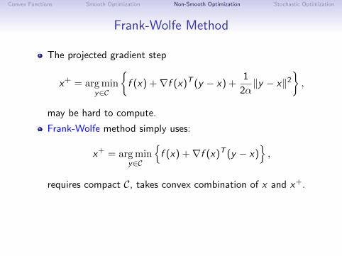
Frank-Wolfe Method
The projected gradient step
x+ = argminy∈C
f (x) +∇f (x)T (y − x) +
1
2α‖y − x‖2
,
may be hard to compute.
Frank-Wolfe method simply uses:
x+ = argminy∈C
f (x) +∇f (x)T (y − x)
,
requires compact C, takes convex combination of x and x+.
Iterate can be written as convex combination of vertices of C.
O(1/t) rate for smooth convex objectives, some linearconvergence results for smooth and strongly-convex.
Convex Functions Smooth Optimization Non-Smooth Optimization Stochastic Optimization
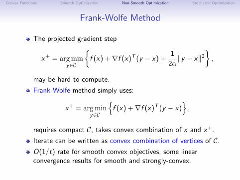
Frank-Wolfe Method
The projected gradient step
x+ = argminy∈C
f (x) +∇f (x)T (y − x) +
1
2α‖y − x‖2
,
may be hard to compute.
Frank-Wolfe method simply uses:
x+ = argminy∈C
f (x) +∇f (x)T (y − x)
,
requires compact C, takes convex combination of x and x+.
Iterate can be written as convex combination of vertices of C.
O(1/t) rate for smooth convex objectives, some linearconvergence results for smooth and strongly-convex.
Convex Functions Smooth Optimization Non-Smooth Optimization Stochastic Optimization
Alternating Direction Method of Multipliers
Alernating direction method of multipliers (ADMM) solves:
minAx+By=c
g(x) + h(y).
Can introduce constraints to convert to this form:
minx=y
g(x) + λ‖y‖1.
Alternate between prox-like operators with respect to x and y .
Useful method for large-scale parallelization.
Convex Functions Smooth Optimization Non-Smooth Optimization Stochastic Optimization
Dual Methods
Stronly-convex problems have smooth duals.
Solve the dual instead of the primal.
SVM non-smooth strongly-convex primal:
minx
CN∑
i=1
max0, 1− biaTi x+
1
2‖x‖2.
SVM smooth dual:
min0≤α≤C
1
2αTAATα−
N∑
i=1
αi
There are many fast methods for bound-constrained problems.
Convex Functions Smooth Optimization Non-Smooth Optimization Stochastic Optimization
Outline
1 Convex Functions
2 Smooth Optimization
3 Non-Smooth Optimization
4 Stochastic Optimization

Convex Functions Smooth Optimization Non-Smooth Optimization Stochastic Optimization
Stochastic Gradient Method
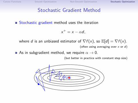
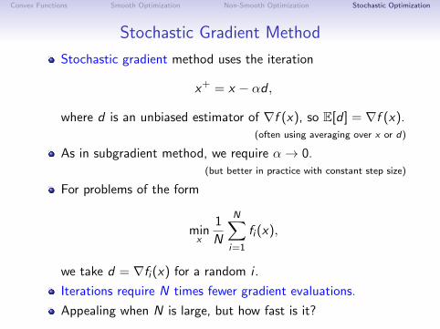
Stochastic gradient method uses the iteration
x+ = x − αd ,
where d is an unbiased estimator of ∇f (x), so E[d ] = ∇f (x).(often using averaging over x or d)
As in subgradient method, we require α→ 0.(but better in practice with constant step size)
Convex Functions Smooth Optimization Non-Smooth Optimization Stochastic Optimization
Stochastic Gradient Method
Stochastic gradient method uses the iteration
x+ = x − αd ,
where d is an unbiased estimator of ∇f (x), so E[d ] = ∇f (x).(often using averaging over x or d)
As in subgradient method, we require α→ 0.(but better in practice with constant step size)
Stochastic vs. deterministic methods
• Minimizing g(!) =1
n
n!
i=1
fi(!) with fi(!) = ""yi, !
!!(xi)#
+ µ"(!)
• Batch gradient descent: !t = !t"1!#tg#(!t"1) = !t"1!
#t
n
n!
i=1
f #i(!t"1)
• Stochastic gradient descent: !t = !t"1 ! #tf#i(t)(!t"1)
Convex Functions Smooth Optimization Non-Smooth Optimization Stochastic Optimization
Stochastic Gradient Method
Stochastic gradient method uses the iteration
x+ = x − αd ,
where d is an unbiased estimator of ∇f (x), so E[d ] = ∇f (x).(often using averaging over x or d)
As in subgradient method, we require α→ 0.(but better in practice with constant step size)
For problems of the form
minx
1
N
N∑
i=1
fi (x),
we take d = ∇fi (x) for a random i .
Iterations require N times fewer gradient evaluations.
Appealing when N is large, but how fast is it?
Convex Functions Smooth Optimization Non-Smooth Optimization Stochastic Optimization
Convex Optimization Zoo
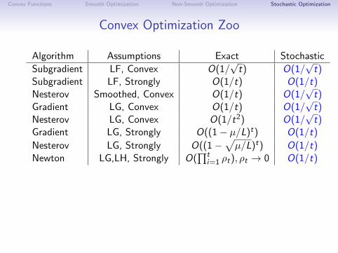
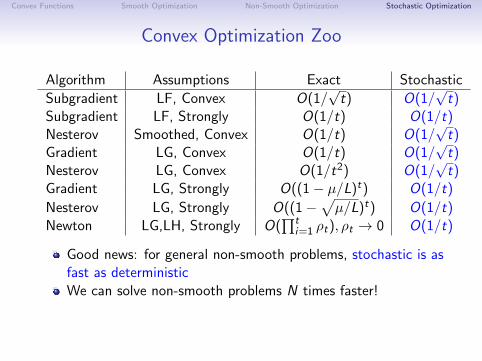
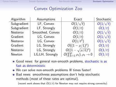
Algorithm Assumptions Exact Stochastic
Subgradient LF, Convex O(1/√
t) O(1/√
t)Subgradient LF, Strongly O(1/t) O(1/t)Nesterov Smoothed, Convex O(1/t) O(1/
√t)
Gradient LG, Convex O(1/t) O(1/√
t)Nesterov LG, Convex O(1/t2) O(1/
√t)
Gradient LG, Strongly O((1− µ/L)t) O(1/t)
Nesterov LG, Strongly O((1−√µ/L)t) O(1/t)
Newton LG,LH, Strongly O(∏t
i=1 ρt), ρt → 0 O(1/t)
Good news: for general non-smooth problems, stochastic is asfast as deterministicWe can solve non-smooth problems N times faster!Bad news: smoothness assumptions don’t help stochasticmethods (most of these rates are optimal).
(recent work shows that O(1/t) for Newton may not require strong convexity)
Convex Functions Smooth Optimization Non-Smooth Optimization Stochastic Optimization
Convex Optimization Zoo
Algorithm Assumptions Exact Stochastic
Subgradient LF, Convex O(1/√
t) O(1/√
t)Subgradient LF, Strongly O(1/t) O(1/t)Nesterov Smoothed, Convex O(1/t) O(1/
√t)
Gradient LG, Convex O(1/t) O(1/√
t)Nesterov LG, Convex O(1/t2) O(1/
√t)
Gradient LG, Strongly O((1− µ/L)t) O(1/t)
Nesterov LG, Strongly O((1−√µ/L)t) O(1/t)
Newton LG,LH, Strongly O(∏t
i=1 ρt), ρt → 0 O(1/t)
Good news: for general non-smooth problems, stochastic is asfast as deterministicWe can solve non-smooth problems N times faster!
Bad news: smoothness assumptions don’t help stochasticmethods (most of these rates are optimal).
(recent work shows that O(1/t) for Newton may not require strong convexity)
Convex Functions Smooth Optimization Non-Smooth Optimization Stochastic Optimization
Convex Optimization Zoo
Algorithm Assumptions Exact Stochastic
Subgradient LF, Convex O(1/√
t) O(1/√
t)Subgradient LF, Strongly O(1/t) O(1/t)Nesterov Smoothed, Convex O(1/t) O(1/
√t)
Gradient LG, Convex O(1/t) O(1/√
t)Nesterov LG, Convex O(1/t2) O(1/
√t)
Gradient LG, Strongly O((1− µ/L)t) O(1/t)
Nesterov LG, Strongly O((1−√µ/L)t) O(1/t)
Newton LG,LH, Strongly O(∏t
i=1 ρt), ρt → 0 O(1/t)
Good news: for general non-smooth problems, stochastic is asfast as deterministicWe can solve non-smooth problems N times faster!Bad news: smoothness assumptions don’t help stochasticmethods (most of these rates are optimal).
(recent work shows that O(1/t) for Newton may not require strong convexity)
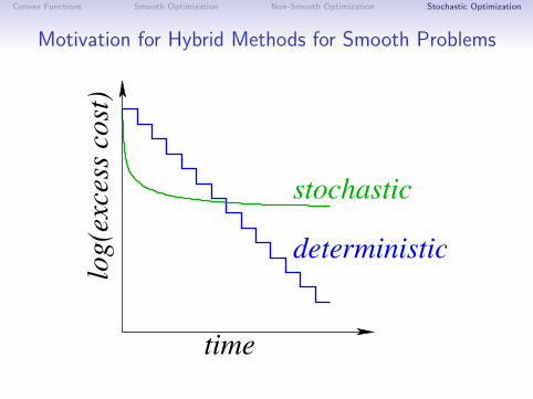
Convex Functions Smooth Optimization Non-Smooth Optimization Stochastic Optimization
Motivation for Hybrid Methods for Smooth Problems
Stochastic vs. deterministic methods
• Goal = best of both worlds: linear rate with O(1) iteration cost
time
log(
exce
ss c
ost)
stochastic
deterministic
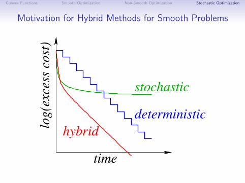
Convex Functions Smooth Optimization Non-Smooth Optimization Stochastic Optimization
Motivation for Hybrid Methods for Smooth Problems
Stochastic vs. deterministic methods
• Goal = best of both worlds: linear rate with O(1) iteration cost
hybridlog(
exce
ss c
ost)
stochastic
deterministic
time
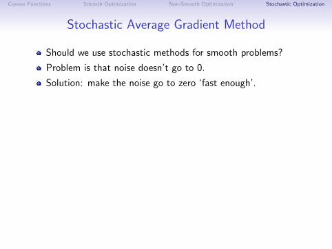
Convex Functions Smooth Optimization Non-Smooth Optimization Stochastic Optimization
Stochastic Average Gradient Method
Should we use stochastic methods for smooth problems?
Problem is that noise doesn’t go to 0.
Solution: make the noise go to zero ‘fast enough’.
Possible in the case of finite data sets:
minx
1
N
N∑
i=1
fi (x),
Stochastic average gradient (SAG) method:
x+ = x − α
N
N∑
i=1
yi ,
on each iteration replace a random yi with ∇fi (x).
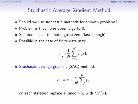
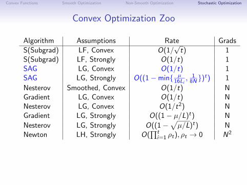
Convex Functions Smooth Optimization Non-Smooth Optimization Stochastic Optimization
Convex Optimization Zoo
Algorithm Assumptions Rate Grads
S(Subgrad) LF, Convex O(1/√
t) 1S(Subgrad) LF, Strongly O(1/t) 1SAG LG, Convex O(1/t) 1SAG LG, Strongly O((1−min µ
16Li, 1
8N )t) 1
Nesterov Smoothed, Convex O(1/t) NGradient LG, Convex O(1/t) NNesterov LG, Convex O(1/t2) NGradient LG, Strongly O((1− µ/L)t) N
Nesterov LG, Strongly O((1−√µ/L)t) N
Newton LH, Strongly O(∏t
i=1 ρt), ρt → 0 N2
Li is the Lipschitz constant over all f ′i (Li ≥ L).SAG has a similar speed to the gradient method, but onlylooks at one training example per iteration.Recent work gives prox, ADMM, and memory-free variants.
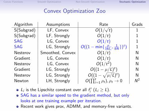
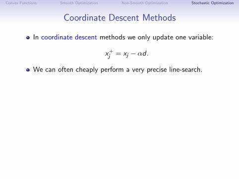
Convex Functions Smooth Optimization Non-Smooth Optimization Stochastic Optimization
Coordinate Descent Methods
In coordinate descent methods we only update one variable:
x+j = xj − αd .
We can often cheaply perform a very precise line-search.
The steepest descent choice is j = argminj∇j f (x).(but only efficient to calculate in some special cases)
Choosing a random j has the same convergence rate.
Faster rate if j sampled according to Lipschitz constants.
Various extensions:
Accelerated version (may lose sparsity of update)Projected coordinate descent (product constraints)Frank-Wolfe coordinate descent (product constraints)Proximal coordinate descent (separable non-smooth term)
(exact step size for `1-regularized least squares)
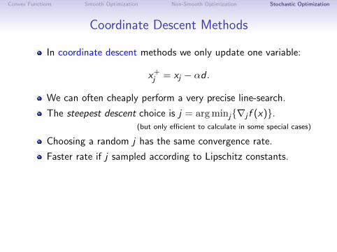
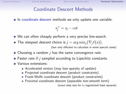
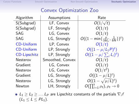
Convex Functions Smooth Optimization Non-Smooth Optimization Stochastic Optimization
Convex Optimization Zoo
Algorithm Assumptions Rate
S(Subgrad) LF, Convex O(1/√
t)S(Subgrad) LF, Strongly O(1/t)SAG LG, Convex O(1/t)SAG LG, Strongly O((1−min µ
16Li, 1
8N )t)CD-Uniform LP, Convex O(1/t)CD-Uniform LP, Strongly O((1− µ/L1P)t)CD-Lipschitz LP, Strongly O((1− µ/∑i Li )
t)Nesterov Smoothed, Convex O(1/t)Gradient LG, Convex O(1/t)Nesterov LG, Convex O(1/t2)Gradient LG, Strongly O((1− µ/L)t)
Nesterov LG, Strongly O((1−√µ/L)t)
Newton LH, Strongly O(∏t
i=1 ρt), ρt → 0
L1 ≥ L2 ≥ . . . LP are Lipschitz constants of the partials ∇i f(L1 ≤ L ≤ PL1).
Convex Functions Smooth Optimization Non-Smooth Optimization Stochastic Optimization
References
A reference to start with for each part:
Part 1: Convex Optimization (Boyd and Vandenberghe)Part 2: Introductory Lectures on Convex Optimization(Nesterov)Part 3: Convex Optimization Theory (Bertsekas)Part 4: Efficient Methods in Convex Programming(Nemirovski)
E-mail me for the other references (mark.schmidt@sfu)
Come talk to me in TASC 9404.
For tutorial material and code:http://www.di.ens.fr/~mschmidt/MLSS
Come join the MLRG:http://www.di.ens.fr/~mschmidt/MLRG.html