Convex Optimization - UAB Barcelonamat.uab.cat/~alseda/MasterOpt/vandenberghe_1_2.pdf · Convex optimization problem minimize f0(x) subject to fi(x) ≤ 0, i = 1,...,m Ax = b f0,

Convex Optimization

Lieven Vandenberghe

University of California, Los Angeles

Tutorial lectures, Machine Learning Summer School

University of Cambridge, September 3-4, 2009

Sources:

• Boyd & Vandenberghe, Convex Optimization, 2004

• Courses EE236B, EE236C (UCLA), EE364A, EE364B (Stephen Boyd, Stanford Univ.)

Convex optimization — MLSS 2009

Introduction

• mathematical optimization, modeling, complexity

• convex optimization

• recent history

1

Mathematical optimization

minimize f0(x1, . . . , xn)

subject to f1(x1, . . . , xn) ≤ 0. . .fm(x1, . . . , xn) ≤ 0

• x = (x1, x2, . . . , xn) are decision variables

• f0(x1, x2, . . . , xn) gives the cost of choosing x

• inequalities give constraints that x must satisfy

a mathematical model of a decision, design, or estimation problem

Introduction 2

Limits of mathematical optimization

• how realistic is the model, and how certain are we about it?

• is the optimization problem tractable by existing numerical algorithms?

Optimization research

• modeling

generic techniques for formulating tractable optimization problems

• algorithms

expand class of problems that can be efficiently solved

Introduction 3

Complexity of nonlinear optimization

• the general optimization problem is intractable

• even simple looking optimization problems can be very hard

Examples

• quadratic optimization problem with many constraints

• minimizing a multivariate polynomial

Introduction 4

The famous exception: Linear programming

minimize cTx =n∑

i=1

cixi

subject to aTi x ≤ bi, i = 1, . . . , m

• widely used since Dantzig introduced the simplex algorithm in 1948

• since 1950s, many applications in operations research, networkoptimization, finance, engineering,. . .

• extensive theory (optimality conditions, sensitivity, . . . )

• there exist very efficient algorithms for solving linear programs

Introduction 5

Solving linear programs

• no closed-form expression for solution

• widely available and reliable software

• for some algorithms, can prove polynomial time

• problems with over 105 variables or constraints solved routinely

Introduction 6

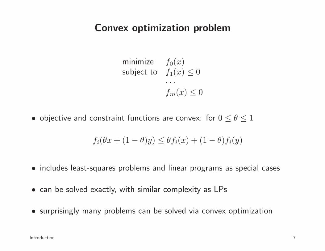
Convex optimization problem

minimize f0(x)subject to f1(x) ≤ 0

· · ·fm(x) ≤ 0

• objective and constraint functions are convex: for 0 ≤ θ ≤ 1

fi(θx + (1 − θ)y) ≤ θfi(x) + (1 − θ)fi(y)

• includes least-squares problems and linear programs as special cases

• can be solved exactly, with similar complexity as LPs

• surprisingly many problems can be solved via convex optimization

Introduction 7

History

• 1940s: linear programming

minimize cTxsubject to aT

i x ≤ bi, i = 1, . . . , m

• 1950s: quadratic programming

• 1960s: geometric programming

• 1990s: semidefinite programming, second-order cone programming,quadratically constrained quadratic programming, robust optimization,sum-of-squares programming, . . .

Introduction 8

New applications since 1990

• linear matrix inequality techniques in control

• circuit design via geometric programming

• support vector machine learning via quadratic programming

• semidefinite programming relaxations in combinatorial optimization

• ℓ1-norm optimization for sparse signal reconstruction

• applications in structural optimization, statistics, signal processing,communications, image processing, computer vision, quantuminformation theory, finance, . . .

Introduction 9

Algorithms

Interior-point methods

• 1984 (Karmarkar): first practical polynomial-time algorithm

• 1984-1990: efficient implementations for large-scale LPs

• around 1990 (Nesterov & Nemirovski): polynomial-time interior-pointmethods for nonlinear convex programming

• since 1990: extensions and high-quality software packages

First-order algorithms

• similar to gradient descent, but with better convergence properties

• based on Nesterov’s ‘optimal’ methods from 1980s

• extend to certain nondifferentiable or constrained problems

Introduction 10

Outline

• basic theory

– convex sets and functions– convex optimization problems– linear, quadratic, and geometric programming

• cone linear programming and applications

– second-order cone programming– semidefinite programming

• some recent developments in algorithms (since 1990)

– interior-point methods– fast gradient methods

10


Convex sets and functions

• definition

• basic examples and properties

• operations that preserve convexity

11

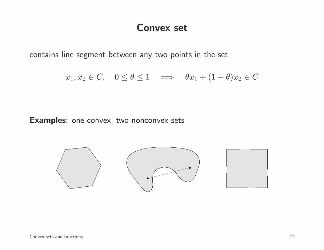
Convex set

contains line segment between any two points in the set

x1, x2 ∈ C, 0 ≤ θ ≤ 1 =⇒ θx1 + (1 − θ)x2 ∈ C

Examples: one convex, two nonconvex sets

Convex sets and functions 12

Examples and properties

• solution set of linear equations Ax = b (affine set)

• solution set of linear inequalities Ax � b (polyhedron)

• norm balls {x | ‖x‖ ≤ R} and norm cones {(x, t) | ‖x‖ ≤ t}

• set of positive semidefinite matrices Sn+ = {X ∈ Sn | X � 0}

• image of a convex set under a linear transformation is convex

• inverse image of a convex set under a linear transformation is convex

• intersection of convex sets is convex


Example of intersection property

C = {x ∈ Rn | |p(t)| ≤ 1 for |t| ≤ π/3}

where p(t) = x1 cos t + x2 cos 2t + · · · + xn cos nt

0 π/3 2π/3 π

−1

0

1

t

p(t

)

x1

x2 C

−2 −1 0 1 2−2

−1

0

1

2

C is intersection of infinitely many halfspaces, hence convex


Convex function

domain dom f is a convex set and

f(θx + (1 − θ)y) ≤ θf(x) + (1 − θ)f(y)

for all x, y ∈ dom f , 0 ≤ θ ≤ 1

(x, f(x))

(y, f(y))

f is concave if −f is convex


Epigraph and sublevel set

Epigraph: epi f = {(x, t) | x ∈ dom f, f(x) ≤ t}

a function is convex if and only itsepigraph is a convex set

epi f

f

Sublevel sets: Cα = {x ∈ dom f | f(x) ≤ α}

the sublevel sets of a convex function are convex (converse is false)


Examples

• exp x, − log x, x log x are convex

• xα is convex for x > 0 and α ≥ 1 or α ≤ 0; |x|α is convex for α ≥ 1

• quadratic-over-linear function xTx/t is convex in x, t for t > 0

• geometric mean (x1x2 · · ·xn)1/n is concave for x � 0

• log det X is concave on set of positive definite matrices

• log(ex1 + · · · exn) is convex

• linear and affine functions are convex and concave

• norms are convex


Differentiable convex functions

differentiable f is convex if and only if dom f is convex and

f(y) ≥ f(x) + ∇f(x)T (y − x) for all x, y ∈ dom f

(x, f(x))

f(y)

f(x) + ∇f(x)T (y − x)

twice differentiable f is convex if and only if dom f is convex and

∇2f(x) � 0 for all x ∈ dom f


Operations that preserve convexity

methods for establishing convexity of a function

1. verify definition

2. for twice differentiable functions, show ∇2f(x) � 0

3. show that f is obtained from simple convex functions by operationsthat preserve convexity

• nonnegative weighted sum• composition with affine function• pointwise maximum and supremum• composition• minimization• perspective


Positive weighted sum & composition with affine function

Nonnegative multiple: αf is convex if f is convex, α ≥ 0

Sum: f1 + f2 convex if f1, f2 convex (extends to infinite sums, integrals)

Composition with affine function: f(Ax + b) is convex if f is convex

Examples

• log barrier for linear inequalities

f(x) = −m∑

i=1

log(bi − aTi x)

• (any) norm of affine function: f(x) = ‖Ax + b‖


Pointwise maximum

f(x) = max{f1(x), . . . , fm(x)}

is convex if f1, . . . , fm are convex

Example: sum of r largest components of x ∈ Rn

f(x) = x[1] + x[2] + · · · + x[r]

is convex (x[i] is ith largest component of x)

proof:

f(x) = max{xi1 + xi2 + · · · + xir | 1 ≤ i1 < i2 < · · · < ir ≤ n}


Pointwise supremum

g(x) = supy∈A

f(x, y)

is convex if f(x, y) is convex in x for each y ∈ A

Example: maximum eigenvalue of symmetric matrix

λmax(X) = sup‖y‖2=1

yTXy


Composition with scalar functions

composition of g : Rn → R and h : R → R:

f(x) = h(g(x))

f is convex if

g convex, h convex and nondecreasingg concave, h convex and nonincreasing

(if we assign h(x) = ∞ for x ∈ domh)

Examples

• exp g(x) is convex if g is convex

• 1/g(x) is convex if g is concave and positive


Vector composition

composition of g : Rn → Rk and h : Rk → R:

f(x) = h(g(x)) = h (g1(x), g2(x), . . . , gk(x))

f is convex if

gi convex, h convex and nondecreasing in each argumentgi concave, h convex and nonincreasing in each argument

(if we assign h(x) = ∞ for x ∈ domh)

Examples

• ∑mi=1 log gi(x) is concave if gi are concave and positive

• log∑m

i=1 exp gi(x) is convex if gi are convex


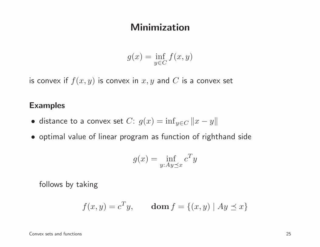
Minimization

g(x) = infy∈C

f(x, y)

is convex if f(x, y) is convex in x, y and C is a convex set

Examples

• distance to a convex set C: g(x) = infy∈C ‖x − y‖• optimal value of linear program as function of righthand side

g(x) = infy:Ay�x

cTy

follows by taking

f(x, y) = cTy, dom f = {(x, y) | Ay � x}


Perspective

the perspective of a function f : Rn → R is the function g : Rn ×R → R,

g(x, t) = tf(x/t)

g is convex if f is convex on dom g = {(x, t) | x/t ∈ dom f, t > 0}

Examples

• perspective of f(x) = xTx is quadratic-over-linear function

g(x, t) =xTx

t

• perspective of negative logarithm f(x) = − log x is relative entropy

g(x, t) = t log t − t log x



Convex optimization problems

• standard form

• linear, quadratic, geometric programming

• modeling languages

27

Convex optimization problem

minimize f0(x)subject to fi(x) ≤ 0, i = 1, . . . , m

Ax = b

f0, f1, . . . , fm are convex functions

• feasible set is convex

• locally optimal points are globally optimal

• tractable, both in theory and practice

Convex optimization problems 28

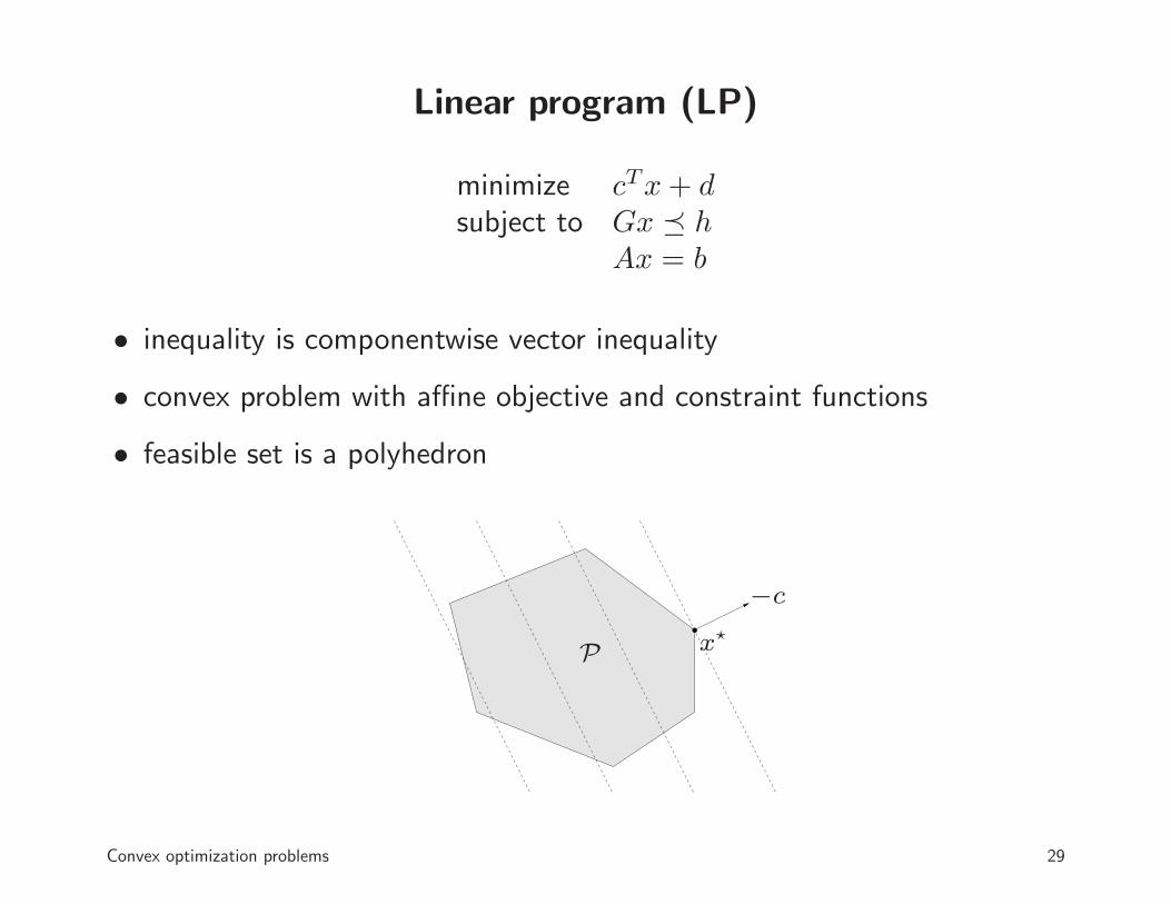
Linear program (LP)

minimize cTx + dsubject to Gx � h

Ax = b

• inequality is componentwise vector inequality

• convex problem with affine objective and constraint functions

• feasible set is a polyhedron

P x⋆

−c


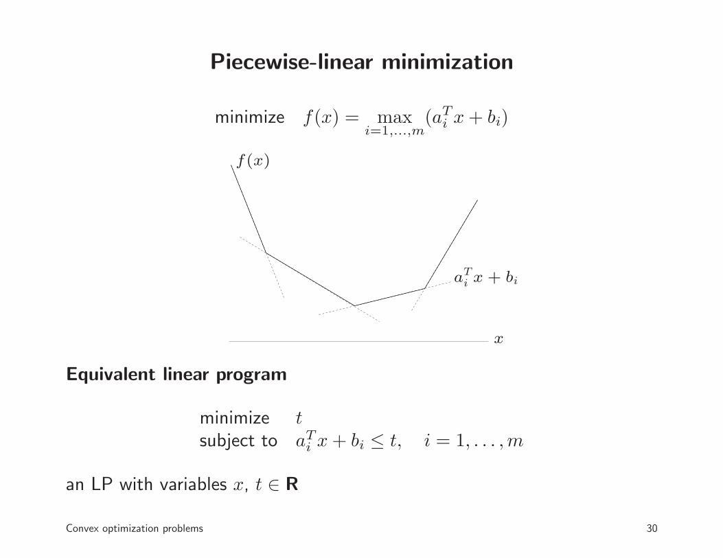
Piecewise-linear minimization

minimize f(x) = maxi=1,...,m

(aTi x + bi)

x

aTi x + bi

f(x)

Equivalent linear program

minimize tsubject to aT

i x + bi ≤ t, i = 1, . . . , m

an LP with variables x, t ∈ R


Linear discrimination

separate two sets of points {x1, . . . , xN}, {y1, . . . , yM} by a hyperplane

aTxi + b > 0, i = 1, . . . , N

aTyi + b < 0, i = 1, . . . , M

homogeneous in a, b, hence equivalent to the linear inequalities (in a, b)

aTxi + b ≥ 1, i = 1, . . . , N, aTyi + b ≤ −1, i = 1, . . . , M


Approximate linear separation of non-separable sets

minimize

N∑

i=1

max{0, 1 − aTxi − b} +

M∑

i=1

max{0, 1 + aTyi + b}

• a piecewise-linear minimization problem in a, b; equivalent to an LP

• can be interpreted as a heuristic for minimizing #misclassified points


ℓ1-Norm and ℓ∞-norm minimization

ℓ1-Norm approximation and equivalent LP (‖y‖1 =∑

k |yk|)

minimize ‖Ax − b‖1 minimize

n∑

i=1

yi

subject to −y � Ax − b � y

ℓ∞-Norm approximation (‖y‖∞ = maxk |yk|)

minimize ‖Ax − b‖∞ minimize ysubject to −y1 � Ax − b � y1

(1 is vector of ones)


Quadratic program (QP)

minimize (1/2)xTPx + qTx + rsubject to Gx � h

Ax = b

• P ∈ Sn+, so objective is convex quadratic

• minimize a convex quadratic function over a polyhedron

P

x⋆

−∇f0(x⋆)


Linear program with random cost

minimize cTxsubject to Gx � h

• c is random vector with mean c and covariance Σ

• hence, cTx is random variable with mean cTx and variance xTΣx

Expected cost-variance trade-off

minimize E cTx + γ var(cTx) = cTx + γxTΣxsubject to Gx � h

γ > 0 is risk aversion parameter


Robust linear discrimination

H1 = {z | aTz + b = 1}H2 = {z | aTz + b = −1}

distance between hyperplanes is 2/‖a‖2

to separate two sets of points by maximum margin,

minimize ‖a‖22 = aTa

subject to aTxi + b ≥ 1, i = 1, . . . , NaTyi + b ≤ −1, i = 1, . . . , M

a quadratic program in a, b


Support vector classifier

min. γ‖a‖22 +

N∑

i=1

max{0, 1 − aTxi − b} +

M∑

i=1

max{0, 1 + aTyi + b}

γ = 0 γ = 10

equivalent to a QP


Sparse signal reconstruction

• signal x of length 1000

• ten nonzero components

0 200 400 600 800 1000

-2

-1

0

1

2

reconstruct signal from m = 100 random noisy measurements

b = Ax + v

(Aij ∼ N (0, 1) i.i.d. and v ∼ N (0, σ2I) with σ = 0.01)


ℓ2-Norm regularization

minimize ‖Ax − b‖22 + γ‖x‖2

2

a least-squares problem

0 200 400 600 800 1000

-2

-1

0

1

2

0 200 400 600 800 1000

-2

-1

0

1

2

left: exact signal x; right: 2-norm reconstruction


ℓ1-Norm regularization

minimize ‖Ax − b‖22 + γ‖x‖1

equivalent to a QP

0 200 400 600 800 1000

-2

-1

0

1

2

0 200 400 600 800 1000

-2

-1

0

1

2

left: exact signal x; right: 1-norm reconstruction


Geometric programming

Posynomial function:

f(x) =K∑

k=1

ckxa1k1 x

a2k2 · · ·xank

n , dom f = Rn++

with ck > 0

Geometric program (GP)


with fi posynomial


Geometric program in convex form

change variables toyi = log xi,

and take logarithm of cost, constraints

Geometric program in convex form:

minimize log

(

K∑

k=1

exp(aT0ky + b0k)

)

subject to log

(

K∑

k=1

exp(aTiky + bik)

)

≤ 0, i = 1, . . . , m

bik = log cik


Modeling software

Modeling packages for convex optimization

• CVX, Yalmip (Matlab)

• CVXMOD (Python)

assist in formulating convex problems by automating two tasks:

• verifying convexity from convex calculus rules

• transforming problem in input format required by standard solvers

Related packages

general purpose optimization modeling: AMPL, GAMS


CVX example

minimize ‖Ax − b‖1

subject to −0.5 ≤ xk ≤ 0.3, k = 1, . . . , n

Matlab code

A = randn(5, 3); b = randn(5, 1);

cvx_begin

variable x(3);

minimize(norm(A*x - b, 1))

subject to

-0.5 <= x;

x <= 0.3;

cvx_end

• between cvx_begin and cvx_end, x is a CVX variable

• after execution, x is Matlab variable with optimal solution



Cone programming

• generalized inequalities

• second-order cone programming

• semidefinite programming

45

Cone linear program

minimize cTxsubject to Gx �K h

Ax = b

• y �K z means z − y ∈ K, where K is a proper convex cone

• extends linear programming (K = Rm+ ) to nonpolyhedral cones

• popular as standard format for nonlinear convex optimization

• theory and algorithms very similar to linear programming

Cone programming 46

Second-order cone program (SOCP)

minimize fTxsubject to ‖Aix + bi‖2 ≤ cT

i x + di, i = 1, . . . , m

• ‖ · ‖2 is Euclidean norm ‖y‖2 =√

y21 + · · · + y2

n

• constraints are nonlinear, nondifferentiable, convex

constraints are inequalitiesw.r.t. second-order cone:

{

y∣

∣

∣

√

y21 + · · · + y2

p−1 ≤ yp

}

y1y2

y3

−1

0

1

−1

0

10

0.5

1

Cone programming 47

Examples of SOC-representable constraints

Convex quadratic constraint (A = LLT positive definite)

xTAx + 2bTx + c ≤ 0 ⇐⇒∥

∥LTx + L−1b∥

∥

2≤ (bTA−1b − c)1/2

also extends to positive semidefinite singular A

Hyperbolic constraint

xTx ≤ yz, y, z ≥ 0 ⇐⇒∥

∥

∥

∥

[

2xy − z

]∥

∥

∥

∥

2

≤ y + z, y, z ≥ 0

Cone programming 48

Examples of SOC-representable constraints

Positive powers

x1.5 ≤ t, x ≥ 0 ⇐⇒ ∃z : x2 ≤ tz, z2 ≤ x, x, z ≥ 0

• two hyperbolic constraints can be converted to SOC constraints

• extends to powers xp for rational p ≥ 1

Negative powers

x−3 ≤ t, x > 0 ⇐⇒ ∃z : 1 ≤ tz, z2 ≤ tx, x, z ≥ 0

• two hyperbolic constraints can be converted to SOC constraints

• extends to powers xp for rational p < 0

Cone programming 49

Robust linear program (stochastic)

minimize cTxsubject to prob(aT

i x ≤ bi) ≥ η, i = 1, . . . , m

• ai random and normally distributed with mean ai, covariance Σi

• we require that x satisfies each constraint with probability exceeding η

η = 10% η = 50% η = 90%

Cone programming 50

SOCP formulation

the ‘chance constraint’ prob(aTi x ≤ bi) ≥ η is equivalent to the constraint

aTi x + Φ−1(η)‖Σ1/2

i x‖2 ≤ bi

Φ is the (unit) normal cumulative density function

00

0.5

1

t

Φ(t

)

η

Φ−1(η)

robust LP is a second-order cone program for η ≥ 0.5

Cone programming 51

Robust linear program (deterministic)


i x ≤ bi for all ai ∈ Ei, i = 1, . . . , m

• ai uncertain but bounded by ellipsoid Ei = {ai + Piu | ‖u‖2 ≤ 1}• we require that x satisfies each constraint for all possible ai

SOCP formulation


i x + ‖PTi x‖2 ≤ bi, i = 1, . . . , m

follows fromsup

‖u‖2≤1

(ai + Piu)Tx = aTi + ‖PT

i x‖2

Cone programming 52

Semidefinite program (SDP)

minimize cTxsubject to x1A1 + x2A2 + · · · + xnAn � B

• A1, A2, . . . , An, B are symmetric matrices

• inequality X � Y means Y − X is positive semidefinite, i.e.,

zT (Y − X)z =∑

i,j

(Yij − Xij)zizj ≥ 0 for all z

• includes many nonlinear constraints as special cases

Cone programming 53

Geometry

[

x yy z

]

� 0

xyz

0

0.5

1

−1

0

10

0.5

1

• a nonpolyhedral convex cone

• feasible set of a semidefinite program is the intersection of the positivesemidefinite cone in high dimension with planes

Cone programming 54

Examples

A(x) = A0 + x1A1 + · · · + xmAm (Ai ∈ Sn)

Eigenvalue minimization (and equivalent SDP)

minimize λmax(A(x)) minimize tsubject to A(x) � tI

Matrix-fractional function

minimize bTA(x)−1bsubject to A(x) � 0

minimize t

subject to

[

A(x) bbT t

]

� 0

Cone programming 55

Matrix norm minimization

A(x) = A0 + x1A1 + x2A2 + · · · + xnAn (Ai ∈ Rp×q)

Matrix norm approximation (‖X‖2 = maxk σk(X))

minimize ‖A(x)‖2 minimize t

subject to

[

tI A(x)T

A(x) tI

]

� 0

Nuclear norm approximation (‖X‖∗ =∑

k σk(X))

minimize ‖A(x)‖∗ minimize (trU + trV )/2

subject to

[

U A(x)T

A(x) V

]

� 0

Cone programming 56

Semidefinite relaxations & randomization

semidefinite programming is increasingly used

• to find good bounds for hard (i.e., nonconvex) problems, via relaxation

• as a heuristic for good suboptimal points, often via randomization

Example: Boolean least-squares

minimize ‖Ax − b‖22

subject to x2i = 1, i = 1, . . . , n

• basic problem in digital communications

• could check all 2n possible values of x ∈ {−1, 1}n . . .

• an NP-hard problem, and very hard in practice

Cone programming 57

Semidefinite lifting

with P = ATA, q = −AT b, r = bT b

‖Ax − b‖22 =

n∑

i,j=1

Pijxixj + 2n∑

i=1

qixi + r

after introducing new variables Xij = xixj

minimize

n∑

i,j=1

PijXij + 2

n∑

i=1

qixi + r

subject to Xii = 1, i = 1, . . . , nXij = xixj, i, j = 1, . . . , n

• cost function and first constraints are linear

• last constraint in matrix form is X = xxT , nonlinear and nonconvex,

. . . still a very hard problem

Cone programming 58

Semidefinite relaxation

replace X = xxT with weaker constraint X � xxT , to obtain relaxation

minimize

n∑

i,j=1

PijXij + 2

n∑

i=1

qixi + r

subject to Xii = 1, i = 1, . . . , n

X � xxT

• convex; can be solved as an semidefinite program

• optimal value gives lower bound for BLS

• if X = xxT at the optimum, we have solved the exact problem

• otherwise, can use randomized rounding

generate z from N (x,X − xxT ) and take x = sign(z)

Cone programming 59

Example

1 1.20

0.1

0.2

0.3

0.4

0.5

‖Ax − b‖2/(SDP bound)

freq

uen

cy

SDP bound LS solution

• feasible set has 2100 ≈ 1030 points

• histogram of 1000 randomized solutions from SDP relaxation

Cone programming 60

Nonnegative polynomial on R

f(t) = x0 + x1t + · · · + x2mt2m ≥ 0 for all t ∈ R

• a convex constraint on x

• holds if and only if f is a sum of squares of (two) polynomials:

f(t) =∑

k

(yk0 + yk1t + · · · + ykmtm)2

=

1...

tm

T∑

k

ykyTk

1...

tm

=

1...

tm

T

Y

1...

tm

where Y =∑

k ykyTk � 0

Cone programming 61

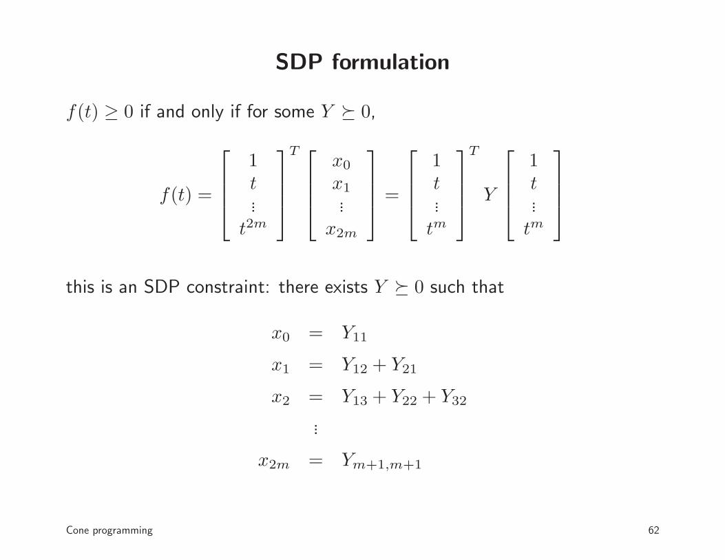
SDP formulation

f(t) ≥ 0 if and only if for some Y � 0,

f(t) =

1t...

t2m

T

x0

x1...

x2m

=

1t...

tm

T

Y

1t...

tm

this is an SDP constraint: there exists Y � 0 such that

x0 = Y11

x1 = Y12 + Y21

x2 = Y13 + Y22 + Y32

...

x2m = Ym+1,m+1

Cone programming 62

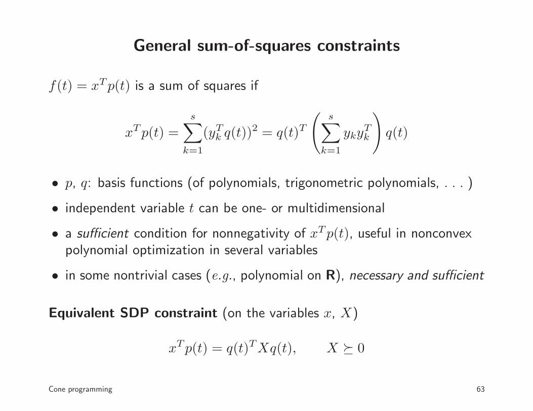
General sum-of-squares constraints

f(t) = xTp(t) is a sum of squares if

xTp(t) =s∑

k=1

(yTk q(t))2 = q(t)T

(

s∑

k=1

ykyTk

)

q(t)

• p, q: basis functions (of polynomials, trigonometric polynomials, . . . )

• independent variable t can be one- or multidimensional

• a sufficient condition for nonnegativity of xTp(t), useful in nonconvexpolynomial optimization in several variables

• in some nontrivial cases (e.g., polynomial on R), necessary and sufficient

Equivalent SDP constraint (on the variables x, X)

xTp(t) = q(t)TXq(t), X � 0

Cone programming 63

Example: Cosine polynomials

f(ω) = x0 + x1 cos ω + · · · + x2n cos 2nω ≥ 0

Sum of squares theorem: f(ω) ≥ 0 for α ≤ ω ≤ β if and only if

f(ω) = g1(ω)2 + s(ω)g2(ω)2

• g1, g2: cosine polynomials of degree n and n − 1

• s(ω) = (cos ω − cos β)(cos α − cos ω) is a given weight function

Equivalent SDP formulation: f(ω) ≥ 0 for α ≤ ω ≤ β if and only if

xTp(ω) = q1(ω)TX1q1(ω) + s(ω)q2(ω)TX2q2(ω), X1 � 0, X2 � 0

p, q1, q2: basis vectors (1, cos ω, cos(2ω), . . .) up to order 2n, n, n − 1

Cone programming 64

Example: Linear-phase Nyquist filter

minimize supω≥ωs|h0 + h1 cos ω + · · · + h2n cos 2nω|

with h0 = 1/M , hkM = 0 for positive integer k

0 0.5 1 1.5 2 2.5 310

−3

10−2

10−1

100

ω

|H(ω

)|

(Example with n = 25, M = 5, ωs = 0.69)

Cone programming 65

SDP formulation

minimize tsubject to −t ≤ H(ω) ≤ t, ωs ≤ ω ≤ π

where H(ω) = h0 + h1 cos ω + · · · + h2n cos 2nω

Equivalent SDP

minimize tsubject to t − H(ω) = q1(ω)TX1q1(ω) + s(ω)q2(ω)TX2q2(ω)

t + H(ω) = q1(ω)TX3q1(ω) + s(ω)q2(ω)TX3q2(ω)

X1 � 0, X2 � 0, X3 � 0, X4 � 0

Variables t, hi (i 6= kM), 4 matrices Xi of size roughly n

Cone programming 66

Chebyshev inequalities

Classical (two-sided) Chebyshev inequality

prob(|X| < 1) ≥ 1 − σ2

• holds for all random X with EX = 0, EX2 = σ2

• there exists a distribution that achieves the bound

Generalized Chebyshev inequalities

give lower bound on prob(X ∈ C), given moments of X

Cone programming 67

Chebyshev inequality for quadratic constraints

• C is defined by quadratic inequalities

C = {x ∈ Rn | xTAix + 2bTi x + ci ≤ 0, i = 1, . . . , m}

• X is random vector with EX = a, EXXT = S

SDP formulation (variables P ∈ Sn, q ∈ Rn, r, τ1, . . . , τm ∈ R)

maximize 1 − tr(SP ) − 2aTq − r

subject to

[

P qqT r − 1

]

� τi

[

Ai bi

bTi ci

]

, τi ≥ 0 i = 1, . . . , m[

P qqT r

]

� 0

optimal value is tight lower bound on prob(X ∈ S)

Cone programming 68

Example

a

C

• a = EX; dashed line shows {x | (x − a)T (S − aaT )−1(x − a) = 1}• lower bound on prob(X ∈ C) is achieved by distribution shown in red

• ellipse is defined by xTPx + 2qTx + r = 1

Cone programming 69

Detection example

x = s + v

• x ∈ Rn: received signal

• s: transmitted signal s ∈ {s1, s2, . . . , sN} (one of N possible symbols)

• v: noise with E v = 0, E vvT = σ2I

Detection problem: given observed value of x, estimate s

Cone programming 70

Example (N = 7): bound on probability of correct detection of s1 is 0.205

s1

s2

s3

s4

s5s6

s7

dots: distribution with probability of correct detection 0.205

Cone programming 71

Cone programming duality

Primal and dual cone program

P: minimize cTxsubject to Ax �K b

D: maximize −bTzsubject to ATz + c = 0

z �K∗ 0

• optimal values are equal (if primal or dual is strictly feasible)

• dual inequality is with respect to the dual cone

K∗ = {z | xTz ≥ 0 for all x ∈ K}

• K = K∗ for linear, second-order cone, semidefinite programming

Applications: optimality conditions, sensitivity analysis, algorithms, . . .

Cone programming 72



• Newton’s method

• barrier method

• primal-dual interior-point methods

• problem structure

73

Equality-constrained convex optimization

minimize f(x)subject to Ax = b

f twice continuously differentiable and convex

Optimality (Karush-Kuhn-Tucker or KKT) condition

∇f(x) + ATy = 0, Ax = b

Example: f(x) = (1/2)xTPx + qTx + r with P � 0

[

P AT

A 0

] [

xy

]

=

[

−qb

]

a symmetric indefinite set of equations, known as a KKT system

Interior-point methods 74

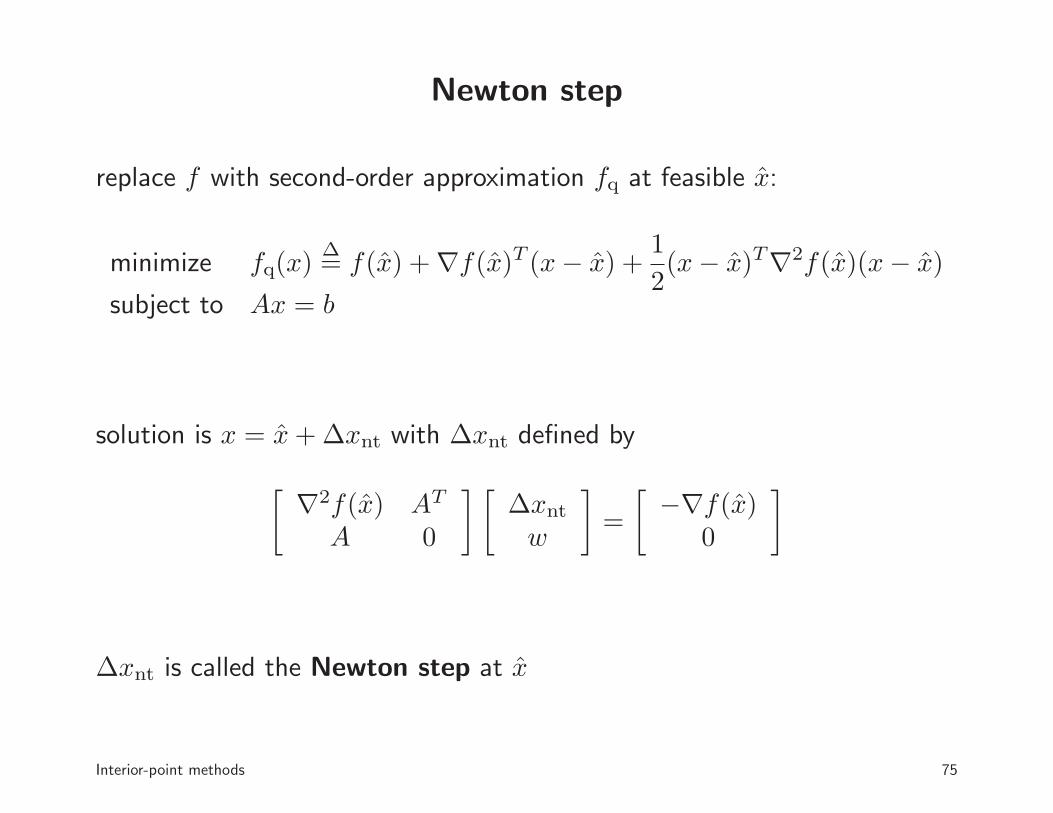
Newton step

replace f with second-order approximation fq at feasible x:

minimize fq(x)∆= f(x) + ∇f(x)T (x − x) +

1

2(x − x)T∇2f(x)(x − x)

subject to Ax = b

solution is x = x + ∆xnt with ∆xnt defined by

[

∇2f(x) AT

A 0

] [

∆xnt

w

]

=

[

−∇f(x)0

]

∆xnt is called the Newton step at x


Interpretation (for unconstrained problem)

x + ∆xnt minimizes 2nd-orderapproximation fq

f

fq

(x, f(x))

(x + ∆xnt, f(x + ∆xnt))

x + ∆xnt solves linearized optimalitycondition

∇fq(x)

= ∇f(x) + ∇2f(x)(x − x)

= 0

f ′

f ′q

(x, f ′(x))

(x + ∆xnt, f ′(x + ∆xnt))


Newton’s algorithm

given starting point x(0) ∈ dom f with Ax(0) = b, tolerance ǫ

repeat for k = 0, 1, . . .

1. compute Newton step ∆xnt at x(k) by solving

[

∇2f(x(k)) AT

A 0

] [

∆xnt

w

]

=

[

−∇f(x(k))0

]

2. terminate if −∇f(x(k))T∆xnt ≤ ǫ3. x(k+1) = x(k) + t∆xnt, with t determined by line search

Comments

• ∇f(x(k))T∆xnt is directional derivative at x(k) in Newton direction

• line search needed to guarantee f(x(k+1)) < f(x(k)), global convergence


Example

f(x) = −n∑

i=1

log(1−x2i )−

m∑

i=1

log(bi − aTi x) (with n = 104, m = 105)

k

f(x

(k) )

−in

ff(x

)

0 5 10 15 20

10−5

100

105

• high accuracy after small number of iterations

• fast asymptotic convergence


Classical convergence analysis

Assumptions (m, L are positive constants)

• f strongly convex: ∇2f(x) � mI

• ∇2f Lipschitz continuous: ‖∇2f(x) −∇2f(y)‖2 ≤ L‖x − y‖2

Summary: two regimes

• damped phase (‖∇f(x)‖2 large): for some constant γ > 0

f(x(k+1)) − f(x(k)) ≤ −γ

• quadratic convergence (‖∇f(x)‖2 small)

‖∇f(x(k))‖2 decreases quadratically


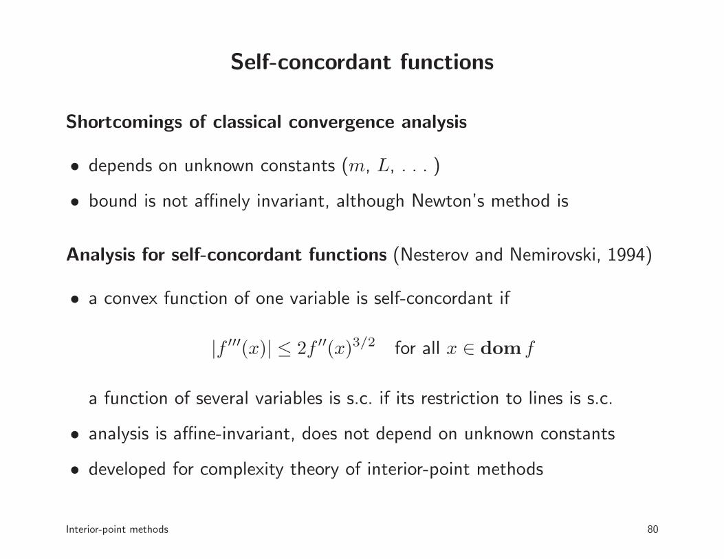
Self-concordant functions

Shortcomings of classical convergence analysis

• depends on unknown constants (m, L, . . . )

• bound is not affinely invariant, although Newton’s method is

Analysis for self-concordant functions (Nesterov and Nemirovski, 1994)

• a convex function of one variable is self-concordant if

|f ′′′(x)| ≤ 2f ′′(x)3/2 for all x ∈ dom f

a function of several variables is s.c. if its restriction to lines is s.c.

• analysis is affine-invariant, does not depend on unknown constants

• developed for complexity theory of interior-point methods



minimize f0(x)subjec to fi(x) ≤ 0, i = 1, . . . , m

Ax = b

functions fi, i = 0, 1, . . . , m, are convex

Basic idea: follow ‘central path’ through interior feasible set to solution

c


General properties

• path-following mechanism relies on Newton’s method

• every iteration requires solving a set of linear equations (KKT system)

• number of iterations small (10–50), fairly independent of problem size

• some versions known to have polynomial worst-case complexity

History

• introduced in 1950s and 1960s

• used in polynomial-time methods for linear programming (1980s)

• polynomial-time algorithms for general convex optimization (ca. 1990)


Reformulation via indicator function


Ax = b

Reformulation

minimize f0(x) +∑m

i=1 I−(fi(x))subject to Ax = b

where I− is indicator function of R−:

I−(u) = 0 if u ≤ 0, I−(u) = ∞ otherwise

• reformulated problem has no inequality constraints

• however, objective function is not differentiable


Approximation via logarithmic barrier

minimize f0(x) − 1

t

m∑

i=1

log(−fi(x))

subject to Ax = b

• for t > 0, −(1/t) log(−u) is a smooth approximation of I−

• approximation improves as t → ∞

u

−lo

g(−

u)/

t

−3 −2 −1 0 1−5

0

5

10


Logarithmic barrier function

φ(x) = −m∑

i=1

log(−fi(x))

with domφ = {x | f1(x) < 0, . . . , fm(x) < 0}

• convex (follows from composition rules and convexity of fi)

• twice continuously differentiable, with derivatives

∇φ(x) =

m∑

i=1

1

−fi(x)∇fi(x)

∇2φ(x) =

m∑

i=1

1

fi(x)2∇fi(x)∇fi(x)T +

m∑

i=1

1

−fi(x)∇2fi(x)


Central path

central path is {x⋆(t) | t > 0}, where x⋆(t) is the solution of

minimize tf0(x) + φ(x)subject to Ax = b

Example: central path for an LP


i x ≤ bi, i = 1, . . . , 6

hyperplane cTx = cTx⋆(t) is tangent tolevel curve of φ through x⋆(t)

c

x⋆ x⋆(10)


Barrier method

given strictly feasible x, t := t(0) > 0, µ > 1, tolerance ǫ > 0

repeat:

1. Centering step. Compute x⋆(t) and set x := x⋆(t)2. Stopping criterion. Terminate if m/t < ǫ3. Increase t. t := µt

• stopping criterion m/t ≤ ǫ guarantees

f0(x) − optimal value ≤ ǫ

(follows from duality)

• typical value of µ is 10–20

• several heuristics for choice of t(0)

• centering usually done using Newton’s method, starting at current x


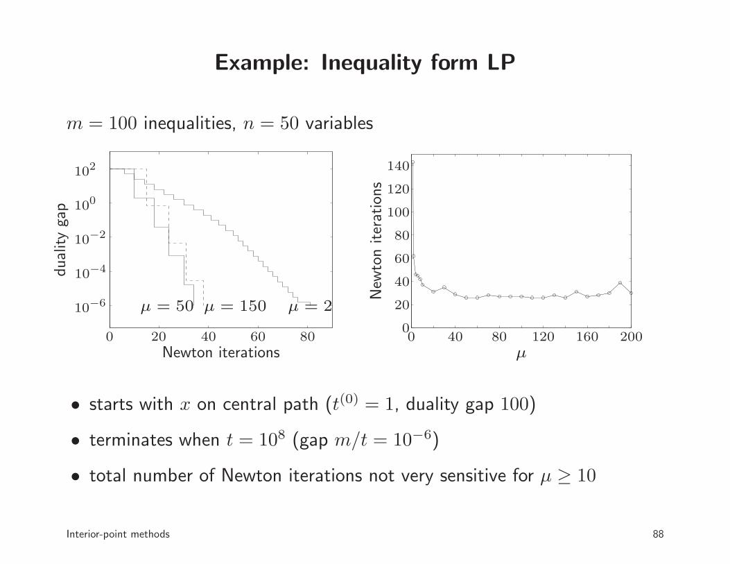
Example: Inequality form LP

m = 100 inequalities, n = 50 variables

Newton iterations

dual

ity

gap

µ = 2µ = 50 µ = 150

0 20 40 60 80

10−6

10−4

10−2

100

102

µ

New

ton

iter

atio

ns

0 40 80 120 160 2000

20

40

60

80

100

120

140

• starts with x on central path (t(0) = 1, duality gap 100)

• terminates when t = 108 (gap m/t = 10−6)

• total number of Newton iterations not very sensitive for µ ≥ 10


Family of standard LPs

minimize cTxsubject to Ax = b, x � 0

A ∈ Rm×2m; for each m, solve 100 randomly generated instances

m

New

ton

iter

atio

ns

101 102 10315

20

25

30

35

number of iterations grows very slowly as m ranges over a 100 : 1 ratio


Second-order cone programming

minimize fTxsubject to ‖Aix + bi‖2 ≤ cT

i x + di, i = 1, . . . , m


φ(x) = −m∑

i=1

log(

(cTi x + di)

2 − ‖Aix + bi‖22

)

• a convex function

• log(v2 − uTu) is ‘logarithm’ for 2nd-order cone {(u, v) | ‖u‖2 ≤ v}

Barrier method: follows central path x⋆(t) = argmin(tfTx + φ(x))


Example

50 variables, 50 second-order cone constraints in R6

Newton iterations

dual

ity

gap

µ = 2µ = 50 µ = 200

0 20 40 60 80

10−6

10−4

10−2

100

102

µ

New

ton

iter

atio

ns

20 60 100 140 1800

40

80

120


Semidefinite programming

minimize cTxsubject to x1A1 + · · · + xnAn � B


φ(x) = − log det(B − x1A1 − · · · − xnAn)

• a convex function

• log det X is ‘logarithm’ for p.s.d. cone

Barrier method: follows central path x⋆(t) = argmin(tfTx + φ(x))


Example

100 variables, one linear matrix inequality in S100

Newton iterations

dual

ity

gap

µ = 2µ = 50µ = 150

0 20 40 60 80 100

10−6

10−4

10−2

100

102

µ

New

ton

iter

atio

ns

0 20 40 60 80 100 120

20

60

100

140


Complexity of barrier method

Iteration complexity

• can be bounded by polynomial function of problem dimensions (withcorrect formulation, barrier function)

• examples: O(√

m) iteration bound for LP or SOCP with m inequalities,SDP with constraint of order m

• proofs rely on theory of Newton’s method for self-concordant functions

• in practice: #iterations roughly constant as a function of problem size

Linear algebra complexity

dominated by solution of Newton system


Primal-dual interior-point methods

Similarities with barrier method

• follow the same central path

• linear algebra (KKT system) per iteration is similar

Differences

• faster and more robust

• update primal and dual variables in each step

• no distinction between inner (centering) and outer iterations

• include heuristics for adaptive choice of barrier parameter t

• can start at infeasible points

• often exhibit superlinear asymptotic convergence


Software implementations

General-purpose software for nonlinear convex optimization

• several high-quality packages (MOSEK, Sedumi, SDPT3, . . . )

• exploit sparsity to achieve scalability

Customized implementations

• can exploit non-sparse types of problem structure

• often orders of magnitude faster than general-purpose solvers


Example: ℓ1-regularized least-squares

minimize ‖Ax − b‖22 + ‖x‖1

A is m × n (with m ≤ n) and dense

Quadratic program formulation

minimize ‖Ax − b‖22 + 1Tu

subject to −u � x � u

• coefficient of Newton system in interior-point method is

[

ATA 00 0

]

+

[

D1 + D2 D2 − D1

D2 − D1 D1 + D2

]

(D1, D2 positive diagonal)

• very expensive (O(n3)) for large n


Customized implementation

• can reduce Newton equation to solution of a system

(AD−1AT + I)∆u = r

• cost per iteration is O(m2n)

Comparison (seconds on 3.2Ghz machine)

m n custom general-purpose50 100 0.02 0.0550 200 0.03 0.17100 1000 0.32 10.6100 2000 0.71 76.9500 1000 2.5 11.2500 2000 5.5 79.8

general-purpose solver is MOSEK



First-order methods

• gradient method

• Nesterov’s gradient methods

• extensions

99

Gradient method

to minimize a convex differentiable function f : choose x(0) and repeat

x(k) = x(k−1) − tk∇f(x(k−1)), k = 1, 2, . . .

tk is step size (fixed or determined by backtracking line search)

Classical convergence result

• assume ∇f Lipschitz continuous (‖∇f(x) −∇f(y)‖2 ≤ L‖x − y‖2)

• error decreases as 1/k, hence

O

(

1

ǫ

)

iterations

needed to reach accuracy f(x(k)) − f⋆ ≤ ǫ

First-order methods 100

Nesterov’s gradient method

choose x(0); take x(1) = x(0) − t1∇f(x(0)) and for k ≥ 2

y(k) = x(k−1) +k − 2

k + 1(x(k−1) − x(k−2))

x(k) = y(k) − tk∇f(y(k))

• gradient method with ‘extrapolation’

• if f has Lipschitz continuous gradient, error decreases as 1/k2; hence

O

(

1√ǫ

)

iterations

needed to reach accuracy f(x(k)) − f⋆ ≤ ǫ

• many variations; first one published in 1983


Example

minimize log

m∑

i=1

exp(aTi x + bi)

randomly generated data with m = 2000, n = 1000, fixed step size

0 50 100 150 20010-6

10-5

10-4

10-3

10-2

10-1

100

gradientNesterov

k

(f(x

(k) )

−f

⋆)/

|f⋆|


Interpretation of gradient update

x(k) = x(k−1) − tk∇f(x(k−1))

= argminz

(

∇f(x(k−1))Tz +1

tk‖z − x(k−1)‖2

2

)

Interpretation

x(k) minimizes

f(x(k−1)) + ∇f(x(k−1))T (z − x(k−1)) +1

tk‖z − x(k−1)‖2

2

a simple quadratic model of f at x(k−1)


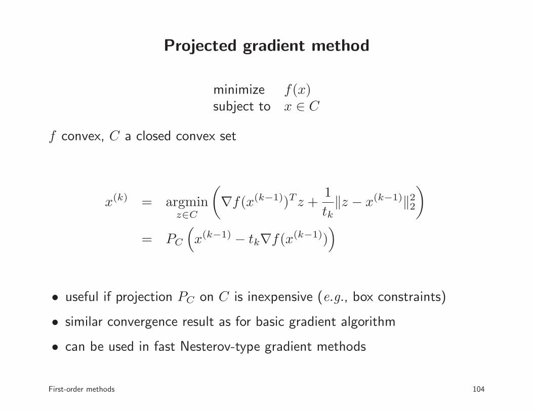
Projected gradient method

minimize f(x)subject to x ∈ C

f convex, C a closed convex set

x(k) = argminz∈C

(

∇f(x(k−1))Tz +1

tk‖z − x(k−1)‖2

2

)

= PC

(

x(k−1) − tk∇f(x(k−1)))

• useful if projection PC on C is inexpensive (e.g., box constraints)

• similar convergence result as for basic gradient algorithm

• can be used in fast Nesterov-type gradient methods


Nonsmooth components

minimize f(x) + g(x)

f , g convex, with f differentiable, g nondifferentiable

x(k) = argminz

(

∇f(x(k−1))Tz + g(x) +1

tk‖z − x(k−1)‖2

2

)

= argminz

(

1

2tk

∥

∥

∥z − x(k−1) + tk∇f(x(k−1))

∥

∥

∥

2

2+ g(z)

)

∆= Stk

(

x(k−1) − tk∇f(x(k−1)))

• gradient step for f followed by ‘thresholding’ operation St

• useful if thresholding is inexpensive (e.g., because g is separable)

• similar convergence result as basic gradient method


Example: ℓ1-norm regularization

minimize f(x) + ‖x‖1

f convex and differentiable

Thresholding operator

St(y) = argminz

(

1

2t‖z − y‖2

2 + ‖z‖1

)

St(y)k =

yk − t yk ≥ t0 −t ≤ yk ≤ tyk + t yk ≤ −t

ykt−t

St(y)k


ℓ1-Norm regularized least-squares

minimize1

2‖Ax − b‖2

2 + ‖x‖1

0 20 40 60 80 10010-7

10-6

10-5

10-4

10-3

10-2

10-1

100

gradientNesterov

k

(f(x

(k) )

−f

⋆)/

f⋆

randomly generated A ∈ R2000×1000; fixed step


Summary: Advances in convex optimization

Theory

new problem classes, robust optimization, convex relaxations, . . .

Applications

new applications in different fields; surprisingly many discovered recently

Algorithms and software

• high-quality general-purpose implementations of interior-point methods

• software packages for convex modeling

• new first-order methods

108

Documents

Convex Optimization - UAB Barcelonamat.uab.cat/~alseda/MasterOpt/vandenberghe_1_2.pdf · Convex optimization problem minimize f0(x) subject to fi(x) ≤ 0, i = 1,...,m Ax = b f0,