Embed Size (px)
Citation preview
CONVERGENCE IN ECONOMIC GROWTH AND ITS
DETERMINANTS: AN EMPIRICAL ANALYSIS
MINA SABBAGHPOOR-FARD
FACULTY OF ECONOMICS AND ADMINISTRATION UNIVERSITY OF MALAYA
KUALA LUMPUR
2013

To My Dearest Mother; Shahla Bohloul Kheibari,
My Dearest Brother; Behrooz Sabaghpour fard and
My Dearest Husband; Hamed Merati.

CONVERGENCE IN ECONOMIC GROWTH AND ITS
DETERMINANTS: AN EMPIRICAL ANALYSIS
MINA SABBAGHPOOR-FARD
THESIS SUBMITTED IN FULFILMENT OF THE REQUIREMENTS
FOR THE DEGREE OF DOCTOR OF PHILOSOPHY
FACULTY OF ECONOMICS AND ADMINISTRATION UNIVERSITY OF MALAYA
KUALA LUMPUR
2013

UNIVERSITI MALAYA
ORIGINAL LITERARY WORK DECLARATION
Name of Candidate: Mina Sabbaghpoor-Fard (I.C/Passport No:J26912126)
Registration/Matric No:EHA090002
Name of Degree: Doctor of Philosophy
Title of Project Paper/Research Report/Dissertation/Thesis (“this Work”):
Convergence in Economic Growth and Its Determinants: An Empirical Analysis
Field of Study: International Economics
I do solemnly and sincerely declare that:
(1) I am the sole author/writer of this Work;
(2) This Work is original;
(3) Any use of any work in which copyright exists was done by way of fair dealing and for
permitted purposes and any excerpt or extract from, or reference to or reproduction of
any copyright work has been disclosed expressly and sufficiently and the title of the
Work and its authorship have been acknowledged in this Work;
(4) I do not have any actual knowledge nor do I ought reasonably to know that the making
of this work constitutes an infringement of any copyright work;
(5) I hereby assign all and every rights in the copyright to this Work to the University of
Malaya (“UM”), who henceforth shall be owner of the copyright in this Work and that
any reproduction or use in any form or by any means whatsoever is prohibited without
the written consent of UM having been first had and obtained;
(6) I am fully aware that if in the course of making this Work I have infringed any
copyright whether intentionally or otherwise, I may be subject to legal action or any
other action as may be determined by UM.
Candidate’s Signature Date
Subscribed and solemnly declared before,
Witness’s Signature Date
Name:
Designation
ii
Abstract
For decades economic growth and its determinants have been the centre of
attention among both theoretical and development economists. Theoretical economists
have built models of economic growth while development economists are concerned as
to how low-income countries can catch up with the rich ones, or, worse, become caught
in a low-income trap. The persistence of poverty in some countries in the world and the
failure to catch up has caused social scientists to not only review and debate the sources
of economic growth but also to take the debate of convergence more seriously and try to
provide different explanations.
Neoclassical growth (NCGM) and new growth (NGM) theories, currently the
main contending schools of thought, try to explain growth sources, and, by extension,
convergence by focusing on capital accumulation and technological change,
respectively. However, empirical studies using either model largely ignore the
importance of institutions, on which there is increasing focus and discussion of
economic performance, and globalization, which affects the economic welfare of
countries. Therefore, in this research we try to reopen the debate of convergence
incorporating these factors in re-estimating the above models. We do this by examining
convergence for three groups of countries, which are classified by income according to
the World Bank classification method, and by applying the GMM method to estimate
the growth models.
The results of this research show that the income level of countries is material
when it comes to both the sources of growth and the speed of convergence. The debate
over which model (NCGM or NGM) is appropriate is not that meaningful. Each model
is appropriate for countries at particular levels of income, but not for the entire income
range. The NCGM, which is believed to be obsolete by many economists, especially
those who espouse the NGM, continues to be relevant for many countries of the world.

iii
Testing the convergence hypothesis in terms of GDP per capita shows that
middle-income countries converge with high-income ones in both models. However,
this only occurs very slowly in low-income countries. Therefore, we can conclude that
income convergence is not monotonic and that an income threshold may need to be
reached before convergence occurs. This shows the existence of a poverty trap.
Investigating the role of institutions and globalization and innovation factors
shows that these factors are the most important drivers of growth for middle-income and
high-income countries but not for low-income countries. However, the effects of these
variables were greatest across middle-income countries compared to high-income
countries, which makes sense for the convergence hypothesis in both classes.
Capital accumulation and secondary schooling are the most important drivers for
low-income countries. This result again alerts us to the existence of an income
threshold. Being more globalized and having stronger institutions does not work for
these groups of countries unless they reach a certain level of income. This is consistent
with the results of other researchers who find that ‘the tide of globalization does not lift
all boats’.

iv
Abstrak
Selama berdekad, pertumbuhan ekonomi dan penentunya menjadi tumpuan di
antara ahli teori ekonomi dan ahli ekonomi pembangunan. Ahli teori ekonomi telah
membina model pertumbuhan ekonomi manakala ahli ekonomi pembangunan pula
prihatin tentang mengapa negara-negara yang berpendapatan rendah boleh mengejar
golongan yang kaya atau lebih teruk lagi terperangkap dalam perangkap penduduk
berpendapatan rendah. Kegigihan daripada belenggu kemiskinan di beberapa negara di
dunia dan kegagalan untuk bersaing telah menyebabkan saintis sosial bukan sahaja
untuk mengkaji dan membahaskan sumber pertumbuhan ekonomi bahkan turut
memberi tumpuan yang lebih serius mengenai perdebatan tentang perubahan itu dan
cuba untuk memberikan penjelasan yang berbeza.
Pertumbuhan neoklasik (NCGM) dan pertumbuhan teori baru (NGM), aliran
pemikiran yang utama pada masa kini adalah, berusaha untuk menjelaskan sumber
pertumbuhan dan mengikut perubahan lanjutan dengan masing-masing memberi
tumpuan kepada pengumpulan modal dan perubahan teknologi. Walau bagaimanapun,
kajian empirikal yang menggunakan kedua-dua model sebahagian besarnya
mengabaikan kepentingan institusi, di mana terdapat tumpuan yang semakin meningkat
dalam perbincangan prestasi ekonomi, dan globalisasi, yang menjejaskan kebajikan
ekonomi negara. Oleh itu, di dalam kajian ini kami berusaha untuk membuka semula
perdebatan tentang perubahan itu dengan menggabungkan faktor-faktor ini dan
menganggarkan semula model-model di atas. Kami berbuat demikian dengan
memeriksa perubahan untuk tiga kumpulan negara-negara yang diklasifikasikan oleh
pendapatan mengikut kaedah klasifikasi Bank Dunia, menggunakan kaedah GMM
untuk menganggarkan pertumbuhan model.

v
Keputusan kajian ini menunjukkan bahawa tahap pendapatan negara adalah penting
apabila ia datang kepada kedua-duanya iaitu sumber pertumbuhan dan kelajuan
perubahan tersebut. Perdebatan ke atas model mana (NCGM atau NGM) yang lebih
sesuai adalah tidak begitu bermakna. Setiap model adalah bersesuaian bagi setiap
negara pada peringkat pendapatan tertentu, tetapi bukan untuk keseluruhan julat
pendapatan. NCGM, yang dipercayai oleh kebanyakan ahli ekonomi, terutama mereka
yang menyokong NGM, menjadi usang, terus menjadi relevan untuk kebanyakan negara
di dunia.
Ujian hipotesis perubahan dari segi KDNK per kapita menunjukkan negara-negara
berpendapatan sederhana akan berubah menjadi orang yang berpendapatan tinggi dalam
kedua-dua model. Walau bagaimanapun, perkara ini berlaku amat perlahan di negara-
negara yang berpendapatan rendah. Oleh itu, kita boleh menyimpulkan bahawa
perubahan pendapatan adalah tidak ekanada dan ambang pendapatan mungkin perlu
dicapai sebelum perubahan berlaku. Ia menunjukkan kewujudan perangkap kemiskinan.
Penyiasatan tentang peranan institusi dan globalisasi dan faktor inovasi
menunjukkan bahawa faktor-faktor ini adalah yang paling penting untuk memacu
pertumbuhan negara berpendapatan sederhana dan berpendapatan tinggi dan bukannya
negara-negara berpendapatan rendah. Walau bagaimanapun, kesan daripada
pembolehubah ini adalah yang terbesar di seluruh negara-negara berpendapatan
sederhana berbanding dengan negara-negara berpendapatan tinggi bagi hipotesis
perubahan yang masuk akal dalam kedua-dua kelas ini.
Pengumpulan modal dan persekolahan menengah adalah perkara yang paling
penting bagi negara-negara berpendapatan rendah. Keputusan ini sekali lagi
mengingatkan kita kepada kewujudan ambang pendapatan. Menjadi lebih global dan
mempunyai institusi yang kuat juga tidak akan berhasil untuk kumpulan negara-negara

vi
sebegini melainkan jika mereka mencapai paras pendapatan tertentu. Ini adalah
konsisten dengan hasil penyelidikan lain yang mendapati bahawa 'arus globalisasi tidak
boleh mengangkat semua bot'.

vii
Acknowledgements
This research project would not have been possible without the support of many
people. I wish to express my gratitude to my supervisors, Dr kee-cheok CHEONG and
Assoc. Professor Dr.Yap Sue Fei who were abundantly helpful and offered invaluable
assistance, support and guidance.
Deepest gratitude is also due to Professor Kim-Leng Goh and Dr. Jay Wysocki,
whose good ideas and advice have always helped me. Also, I would like to thank the
Department of Economics, Faculty of Economics and Administration, University of
Malaya for giving me an opportunity to complete my PhD.
Special thanks also to all my graduate friends, especially Sarala Aikanathan,
Hashem Salarzadeh Janatabadi, Chor Foon Tang, Navaz Naghavi, Babak Barkhordar,
Sara Abbasian, Saeed Nori Neshat and Hamid Reza Ghorbani for sharing the literature
and invaluable assistance. Also not forgetting to my best friends who have always been
there for me.
I would also like to convey thanks to the Institute of Postgraduate Studies (IPS),
especially Professor Mohamed Kheireddine, and Nippon foundation from Japan for
financial support and the scholarship in all these years.
I wishes to express my love and gratitude to my beloved family, especially my
husband; for their understanding and endless love, through the duration of my studies.
viii
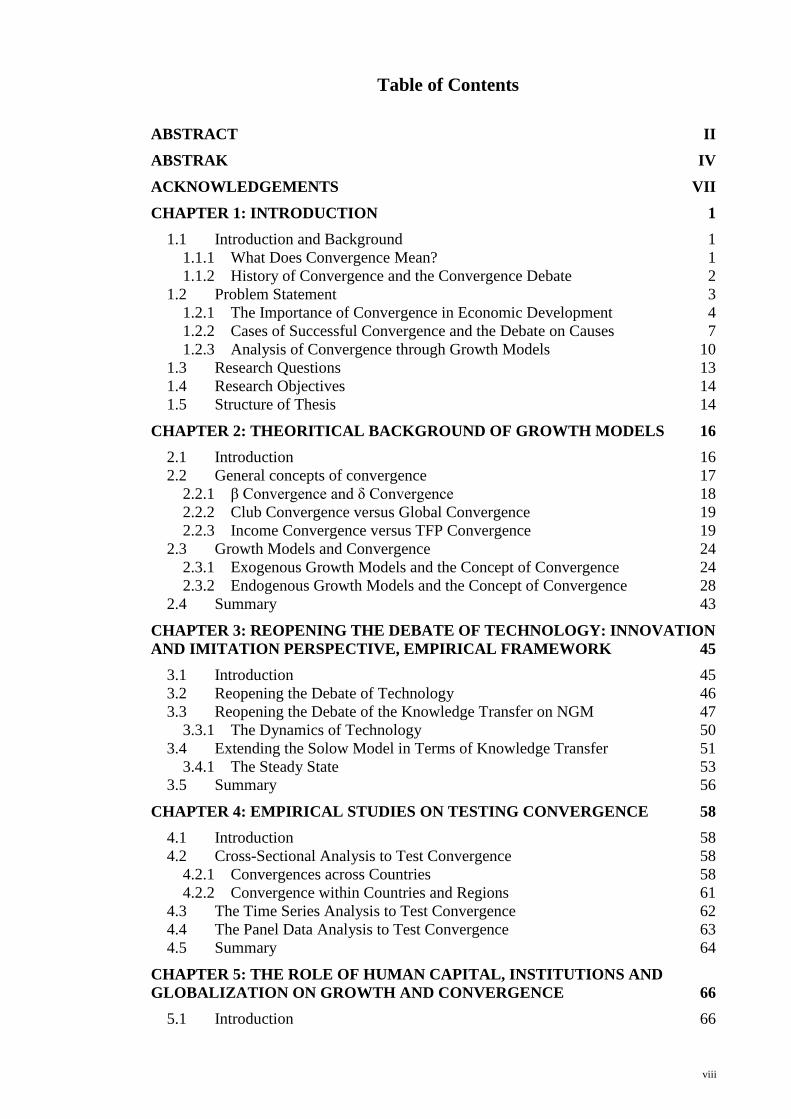
1 Table of Contents
ABSTRACT II
ABSTRAK IV
ACKNOWLEDGEMENTS VII
CHAPTER 1: INTRODUCTION 1
1.1 Introduction and Background 1
1.1.1 What Does Convergence Mean? 1 1.1.2 History of Convergence and the Convergence Debate 2
1.2 Problem Statement 3
1.2.1 The Importance of Convergence in Economic Development 4
1.2.2 Cases of Successful Convergence and the Debate on Causes 7
1.2.3 Analysis of Convergence through Growth Models 10
1.3 Research Questions 13
1.4 Research Objectives 14
1.5 Structure of Thesis 14
CHAPTER 2: THEORITICAL BACKGROUND OF GROWTH MODELS 16
2.1 Introduction 16
2.2 General concepts of convergence 17
2.2.1 β Convergence and δ Convergence 18
2.2.2 Club Convergence versus Global Convergence 19 2.2.3 Income Convergence versus TFP Convergence 19
2.3 Growth Models and Convergence 24
2.3.1 Exogenous Growth Models and the Concept of Convergence 24 2.3.2 Endogenous Growth Models and the Concept of Convergence 28
2.4 Summary 43
CHAPTER 3: REOPENING THE DEBATE OF TECHNOLOGY: INNOVATION
AND IMITATION PERSPECTIVE, EMPIRICAL FRAMEWORK 45
3.1 Introduction 45
3.2 Reopening the Debate of Technology 46
3.3 Reopening the Debate of the Knowledge Transfer on NGM 47
3.3.1 The Dynamics of Technology 50
3.4 Extending the Solow Model in Terms of Knowledge Transfer 51
3.4.1 The Steady State 53 3.5 Summary 56
CHAPTER 4: EMPIRICAL STUDIES ON TESTING CONVERGENCE 58
4.1 Introduction 58
4.2 Cross-Sectional Analysis to Test Convergence 58
4.2.1 Convergences across Countries 58 4.2.2 Convergence within Countries and Regions 61
4.3 The Time Series Analysis to Test Convergence 62
4.4 The Panel Data Analysis to Test Convergence 63
4.5 Summary 64
CHAPTER 5: THE ROLE OF HUMAN CAPITAL, INSTITUTIONS AND
GLOBALIZATION ON GROWTH AND CONVERGENCE 66
5.1 Introduction 66
ix
5.2 History of Human Capital as a Factor Explaining Growth 67
5.3 Institutional Factors in Economic Growth and Convergence 72
5.4 Globalization, Economic Growth and Convergence Progress 78
5.5 Summary 80
CHAPTER 6: RESEARCH METHODOLOGY, MODEL SPECIFICATION AND
DATA 81
6.1 Introduction 81
6.2 Estimation Method 82
6.2.1 A Consistent Estimator for Growth Regressions 85 6.2.2 Data and measurement issues 92 6.2.3 Sources of Data and List of countries 102
6.3 Research Hypotheses 105
CHAPTER 7: ESTIMATION RESULTS 107
7.1 Introduction 107
7.2 Neoclassical growth model 108
7.2.1 Testing β Convergence in First Augmented Solow-Swan Model 109 7.2.2 Testing β Convergence in the Second Augmented Solow-Swan Model 112 7.2.3 δ - Convergence 132
7.3 New Growth Model 133
7.3.1 Testing β Convergence: The Link Between Technological Change and
Convergence in Income 134 7.3.2 φ Convergence 148
7.4 Middle-income Trap: More Testing on Convergence 152
7.5 Summary of Statistical Results 155
7.5.1 Convergence in each Class of Model 155
7.5.2 Impact of Globalization on Economic Growth and Convergence 156
7.5.3 Impact of Institutions on Economic Growth and Convergence 157 7.5.4 Testing the φ convergence 158 7.5.5 Validity of Growth Models: Neoclassical or New Growth Models 159
CHAPTER 8: CONCLUDING REMARKS AND POLICY IMPLICATIONS 161
8.1 Overview 161
8.2 Research Findings: Rate of Convergence in Neoclassical and New Growth
Theory 162
8.3 Contributions of the Study 166
8.4 Limitations of the study 168
8.5 Policy Recommendations 168
8.6 Suggestions for Further Research 170
REFERENCES 172
APPENDIX 180

x
LIST OF FIGURES
Figure 1-0-1: GDP per capita (in constant 2000 USD) dispersion between OECD
countries and Korea 8 Figure 1-0-2: GDP per capita (in constant 2000 USD) dispersion across OECD
countries, Korea, India, China, Brazil and Low-income countries. 8
Figure 2-1: The growth trend of low-income, middle-income and high-income
economies 17 Figure 2-2: Convergence across low-income Countries in terms of GDP per capita and
productivity, 1996–2010. 20 Figure 2-3: Convergence Middle-income Countries in terms of GDP per capita and
productivity, 1996–2010 21
Figure 2-4: Convergence across high-income Countries in terms of GDP per capita and
productivity, 1996–2010 22 Figure 2-5: GDP per capita dispersion in the high-income, Middle-income and low-
income countries, 1980-2010 23 Figure 6-1: New growth model framework 85
Figure 6-2: Neoclassical growth model framework 88 Figure 7-1 Distribution of countries by level of income 153

xi
LIST OF TABLES
Table 6-1: Expected signs of variables 99 Table 6-2: list of Countries in each group 103 Table 7-1 Testing convergence in the first Augmented Solow-Swan Model using
dynamic system GMM 109
Table 7-2 Second Augmented Solow-Swan model in the whole sample using dynamic
system GMM panel data. 113 Table 7-3 Second Augmented Solow-Swan model in high-income countries using
dynamic system GMM panel data 115 Table 7-4 Second Augmented Solow-Swan model in middle-income countries using
dynamic system GMM panel data. 117
Table 7-5 Second Augmented Solow-Swan model in low-income countries using
dynamic system GMM panel data 119 Table 7-6 Speed of Convergence in second Augmented Solow-Swan model, 1996-2010
121 Table 7-7 The results for secondary school enrolment ratio in both models 123
Table 7-8 The results for investment in physical capital in both models 124 Table 7-9 the results for R&D intensity and Number of Scientific Journals in the second
model 125 Table 7-10 The results for FDI and KOF index in second model 126 Table 7-11 The results for Governance indicators in the second model 128
Table 7-12 Results of testing δ convergence in terms of GDP per capita, 1996-2010 132 Table 7-13 Testing β convergence in terms of GDP per capita in the whole sample,
using dynamic system GMM 135 Table 7-14 Testing β convergence in terms of GDP per capita using dynamic System
GMM across High income countries 137 Table 7-15 Dynamic system GMM, testing β convergence in terms of GDP in middle-
income countries. 139 Table 7-16 Testing β convergence in terms of GDP in low-income countries, Using
dynamic system GMM. 140
Table 7-17 Speed of Convergence in New Growth model, 1996-2010 142 Table 7-18 The results of secondary school enrolments ratio in the NG model 145 Table 7-19 The results of investment on physical capital in both models 145
Table 7-20 The results of R&D intensity and Number of scientific Journals in both
models 146
Table 7-21 The results of the KOF index and FDI in both models 147
Table 7-22 The results of Governance indicators in both models 148
Table 7-23: φ convergence in terms of technology dimensions, 1996-2010 150 Table 7-24 countries that have always been in the low-income group between 1985 and
2010 154 Table 8-1 Comparison of Convergence Rate Across Sample Groups Between NCG and
NG Models 163
1
Chapter 1
Introduction
1.1 Introduction and Background
The question of whether poorer countries are converging to the richer ones is an
important issue in development economics, in general, and growth literature, in
particular (P Aghion & Howitt, 1998; P. Aghion & P. Howitt, 2006; R. J. Barro, 1991;
Phelps, 1966; Raiser, Di Tommaso, & Weeks, 2001; J.D. Sachs, 2003). Convergence is
important for developing countries because of the already wide gap between rich and
poor countries and because for some of the latter, this gap is increasing. This process is
also occurring in most of the development that has global significance. Such
development includes increasing the globalization of goods, services, finance, people
and ideas, as well as accelerating technological change. For a better understanding about
the debate of convergence it is helpful to have an initial definition of this term from the
growth literature.
1.1.1 What Does Convergence Mean?
“Poorer countries can grow at a faster rate than rich countries in terms of GDP
per capita and reach to the same steady state” provides a general definition for the term
unconditional convergence from the neoclassical growth theory. In this theory,
developing countries should grow faster because of the diminishing return to scale,
especially for capital. However, later on, during the twentieth century, following the
second industrial revolution, 1860-1865, technological revolution economists started
thinking about catching up in terms of technology and not GDP per capita, and,

2
therefore, the concepts of frontiers or distance and proximity to frontiers became
important in the new growth theories.
1.1.2 History of Convergence and the Convergence Debate
Around 300 hundred years ago, about 1750, the industrial revolution happened
in England and income started to increase. The pattern spread among European
countries, the US, Canada, Australia and New Zealand, and for two hundred years
economic growth was sustained and increased in these areas. The source of this growth
was technology, science, communication, institutions and governance. This increase in
income affected the lives of around 15 per cent of the people in the world (Spence,
2011). Outside this circle, the other countries remained poor, and, therefore, great
divergence happened. However, after World War II, 1945, this growth also started in
developing countries. Of course, at first, it was not massive and it only happened in
some isolated countries, however, after a while, it spread to other countries.
Furthermore, the growth rate became even greater, 7 per cent, compared to industrial
countries that were around 2 per cent during those 200 years. It seems that after two-
hundred years of what has come to be called “the great divergence”(Pomeranz, 2001),
convergence has taken over. What caused this shift to occur? Which factors accelerated
the growth rate in these groups of countries? The interesting part is that,
notwithstanding the shift, some countries are still trapped at the low-income level, and
cannot even catch up with the middle-income countries.
According to the new growth theories developed by P. Aghion and P. Howitt
(2006), and C. Jones (1998), technology plays an important role in explaining the
growth rate of advanced countries and a large proportion of their growth is explained by
technological change. Furthermore, these classes of theoretical models, which were

3
inspired by Schumpeter, argue that being farther away from technology leaders or
advanced countries could be a benefit for the developing and undeveloped countries to
take advantage of this backwardness and grow faster. However, as can be seen in the
reality, this idea of technology catching up is not working for some low-income
countries. They are far away from the technology leaders and even though they have
such an advantage to grow faster they are still in the trap of a low level of income.
1.2 Problem Statement
The persistence of poverty in several countries in the world, and, therefore, the
failure of technological catching up and convergence hypothesis, has led to social
scientists taking the debate of convergence more seriously and encouraged them to
provide different explanations for this behaviour. While some economists, like Bloom,
Sachs, Collier, and Udry (1998), explain the failure using geographical reasons, others,
like R. Nelson (2007) and D. Dollar and Kraay (2004) use the role of institutions and
globalization, respectively. These explanations can be grouped under different theories
of economic growth.
The neoclassical and new growth theories try to explain these differences by
focusing on capital accumulation and technological change, respectively. However,
empirical studies in this area, technological catching up and convergence hypothesis,
largely ignore the importance of institutions and globalization. Therefore, in this
research we try to reopen the debate of convergence according to these shortcomings in
empirical studies, and, by applying a new method of estimation, generalized method of
moments (GMM), re-estimate the models across three different groups of countries that
are classified by their level of income according to the world classification method.

4
1.2.1 The Importance of Convergence in Economic Development
The growth rate of countries is one of the most important concerns of
economists in recent decades, because it is not only about the welfare and level of
standard of living of people, but it is also about having better political and social
positions across different countries (Milanovic & Squire, 2005). Taking a look at the
United States of America (US) could be a good example. Since 1870, the US GDP per
capita increased almost tenfold until 1990. In contrast, the GDP per capita of Africa for
the same period only increased threefold. This rapid growth made the US a superpower
among countries. Recently we can see this kind of rapid growth rate for China and some
other countries and the political movement among them. Indeed, the growth of
latecomers like Korea and Taiwan has excited development economists eager to identify
development “models”. Indeed, the rise of China, India and other members of the
BRICs (Brazil and Russia) are shifting the economic balance of power from the so-
called G7. Therefore, understanding the driving forces of growth is always interesting
for economists. At the same time, these gaps among developed, undeveloped and
developing countries have attracted the attention of economists. Studies have attempted
to determine why some countries are rich while others are poor, and which factors can
accelerate the growth rate of countries to converge to the development level. Such
questions raise the concept of convergence.
Actually, the debate on convergence came into sharp focus when P.M. Romer
(1986) questioned the neoclassical growth models (NCGM) introduced by Solow
(1956). Solow’s models raised the convergence concept. He believed that since there is
a diminishing return to capital and labour, an economy is converging to a unique steady
state, whether it is higher or lower than the equilibrium capital level. Of course, initially
it was all about convergence within a country and later it was extended to across

5
countries. Since this NCGM could not explain the long-run growth path and at the same
time come to a bigger sample, because of different structures, convergence is not
happening or in other words countries are heterogeneous in some aspects and so their
steady state determinants are different. P. Romer (1991) claimed that this class of
model is not accurate and he introduced the new growth theory (NGM): endogenous
growth model. In this new model, P.M. Romer (1986) questioned two main
assumptions of the NCGM: first, diminishing returns to capital and labour, and, second,
exogeneity of technology. By avoiding these two assumptions he could explain the
endogenous long-run growth of economies. In this model, technology is endogenous,
countries can grow in the long-run, and, therefore, there is no convergence across
countries.
However, empirical evidence in the world shows that convergence is happening
and those developing countries are accelerating their growth rate and catching up with
the richer ones. Therefore, Romer’s model also seems to be inadequate. This point is
helpful to understand the interactions across countries among other dimensions like
human capital, institutions and so on. At the same time, Solow’s assumption that
countries with similar economic structures should converge to the same steady state has
also not been borne out in the real world. This was the beginning of the convergence
debate, which created different concepts, methodologies and factors.
One area of development is to refine the specification of models through the
inclusion of new variables in growth models to control the steady state growth path of
different countries. Thus, N. G. Mankiw, D. Romer, and D. N. Weil (1992) introduced
the augmented Solow model to the literature, and, by adding human capital to the
growth model, claimed that 80% of cross country income differences can be explained
by this model. Meanwhile, economists like Redek and Sušjan (2005), F. Caselli, G.

6
Esquivel, and F. Lefort (1996); Easterly and Levine (1997); Nandakumar, Batavia, and
Wague (2004) , and Pomeranz (2001) argue that capital per capita (physical and human)
can only account for a proportion of differences in output per worker, and, instead,
changes in total factor productivity or technological changes can explain the huge
difference. Therefore, total factor productivity (TFP) became the engine behind long-
run growth across countries.
In addition, the endogenous growth model makes it possible to explain these
differences by endogenizing technology, stock of knowledge, through different
channels. Economists have conducted much research in this area concerning through
which channels technology can affect TFP, and, finally, growth. Human capital is one
of the important channels through which technology can affect growth. Economists like
Lucas (1988), pioneered applying human capital in a different way than just investment
in education, like the effect of learning by doing through human capital on growth. By
introducing these spillover effects, other economists tried to contribute to the growth
literature by incorporating other factors that can effect growth through human capital,
such as R&D, technology transfers or imitation, trade and innovation (Eberhardt &
Teal, 2010; J. Ha & P. Howitt, 2007; Harris, 2011; Madsen, 2008).
As can be seen, studies about conditional convergence produced different
important issues that can be important for growth literature. First, by studying
conditional convergence, new stylized facts about growth across several countries can
be produced. Second, undertaking research about convergence highlights the
significance of changing technology across countries, and, therefore, develops new
methodologies and also factors for quantification of these differences. The results of
such quantification are very important since they create different technology based
models, and, like the current study, can also be a motivation to contribute to the

7
literature by applying them in different theories like the neoclassical model.
Furthermore, choosing convergence as the criterion to give validity to growth models
makes this debate more important. Researchers have argued that by testing the
convergence hypothesis the validity of the model can be approved. This argument has
introduced many different methods, models, and concepts, to the growth literature.
1.2.2 Cases of Successful Convergence and the Debate on Causes
To make the concept of convergence clear, first we take a look at some
successful countries in this process and explain how they have escaped from the low-
income trap and catch up with the rich ones. Later we extend it across other countries
and test the convergence hypotheses based on two-definitions highlighted in this study
by employing two growth models.
One good example is Korea, which joined the OECD countries in 1996 (Figure
1-1). In 1965, its GDP per capita was around USD1,351 and although during 18 years
this amount doubled and reached USD3,709 the distinction between OECD and Korea
remained.

8
Figure 1-0-1: GDP per capita (in constant 2000 USD) dispersion between OECD countries and Korea
Note: Author’s calculations
However, around 1996, its GDP per capita accelerated and rose to USD10,119
and, therefore, caught up with the OECD countries, and, finally, Korea joined this
group. Other countries that can also be named as successful in the process of catching
up include China and India.
Figure 1-0-2: GDP per capita (in constant 2000 USD) dispersion across OECD countries, Korea, India,
China, Brazil and Low-income countries.
Note: Author’s calculations
0
2000
4000
6000
8000
10000
12000
14000
16000
18000
19
65
19
67
19
69
19
71
19
73
19
75
19
77
19
79
19
81
19
83
19
85
19
87
19
89
19
91
19
93
19
95
19
97
19
99
20
01
20
03
20
05
20
07
20
09
OECD
Korea
0
2000
4000
6000
8000
10000
12000
14000
16000
18000
19
65
19
68
19
71
19
74
19
77
19
80
19
83
19
86
19
89
19
92
19
95
19
98
20
01
20
04
20
07
20
10
OECD
Korea
India
China
Brazil
low-income

9
The interesting thing about China is that, around 1965, its GDP per capita was
approximately USD100 lower than India, which was around USD192 (Figure 1-2).
However, by late 1980, when some countries agreed to have more liberalized economies
in order to became more prosperous, as figure 1-2 shows, China accelerated its growth
rate and it rose to USD2,425 in 2010 even with the Asian crisis in 1997-98. However,
India could not catch up with the developed countries as fast as China or Korea.
We can extend this question to other countries in the middle-income and low-
income groups as well. Why do these countries not accelerate their growth rate to catch
up and converge with the developed one? Why does poverty persist in some low-
income countries? For instance, in the case of Africa, during the period 1965-1990, on
average, the growth rate of GDP per capita was 0.2 per cent while, in East Asia and the
Pacific the growth rate of GDP per capita was around five per cent (Easterly & Levine,
1997). This poverty persists in African countries in the sense that the levels of income
in the 1990s were the same as in 1970. This empirical evidence of persistence of
poverty in poor countries, on the one hand, and the catching up of some countries with
the developed ones, on the other hand, attracted the attention of economists to
investigate the factors and policies that can affect growth in these countries. This
evidence raises many questions about convergence. Were those countries that were
more successful endowed with better conditions in the beginning? Were there factors
special to these countries that could grow fast? Was it luck? Was it history? Were
there factors that were favourable to growth? Of course, we can say that a part of this
debate is ideological, whether it is the market or the state? However, since this is not the
concern of this study we open this part for further research.

10
1.2.3 Analysis of Convergence through Growth Models
Convergence has been analysed from both a qualitative and quantitative
perspective. Qualitative discussions are framed in terms of poverty and overcoming
barriers to its reduction. Quantitative analysis has been largely based on growth models.
Yet, from the perspective of growth models, convergence is an important but not the
primary objective of investigation, which is to explain why and how economic growth
occurs. Researchers use growth models to examine the convergence hypothesis,
classifying them by type as a basis for comparison, such as unconditional convergence
vs. conditional convergence, income convergence vs. total factor productivity (TFP)
convergence, and global convergence vs. club convergence, etc. Therefore, estimating
convergence equations and the factors that contribute to convergence has become
increasingly popular and convergence or the ability to catch up economically became
the criterion to assess which class of growth models is valid. One of the purposes of this
research is to test whether these different growth model types are mutually exclusive,
and, hence, whether the existing judgment of their validity, convergence hypothesis, is
appropriate. To do so, different growth models and the determinants of growth should
be explained.
Growth models have developed over time. The neoclassical exogenous growth
model (NCGM), which was introduced by Solow (1956) and Swan (1956), was
pioneered in testing the convergence hypothesis. However, subsequently, because of the
shortcomings of this model according to empirical evidence, P.M. Romer (1986) talked
about the endogenous growth model (NGM), which consists of a newer version of the
NCGM as well as the evolutionary growth model of Schumpeter and others. The NGM
was expanded by C. Jones (1998) in the R&D based model, and P Aghion and Howitt
(1998) who talked about the importance of R&D intensity instead of inputs and distance
11
to frontiers. However, at the same time, the Schumpeterian framework ran parallel to
the neoclassical models.
In each of these classes, the channel that brings growth is different. The NGM
studies focused more on catch up technologically, by working more on factors that can
increase total factor productivity as a source of growth rather than factor accumulation,
which is important in NCGM. This is because researchers recognize the limits of factor
accumulation in the efforts of countries to achieve catch-up growth. At the same time,
economists like Redek and Sušjan (2005) supported that most of the differences in
growth rates across countries could be explained by total factor productivity. In these
models, innovation and R&D play a crucial role on productivity growth (J. Ha & P.
Howitt, 2007; Kortum, 1998; Madsen, 2008; Segerstrom, 1998).
In addition, economists like N. G. Mankiw et al. (1992), in their augmented
Solow model, explained the cross country income variations by physical and human
capital accumulation, and not technology change, which was supported by Pääkkönen
(2010) .
How and through which channels technology and factor accumulation can affect
growth in the new growth model and neoclassical model, respectively, are two
important questions in growth literature.
One of the variables that play a crucial role in both NCGM and NGM literature
is human capital. However, the way that these two theories look at this factor is
different. In the neoclassical growth models, human capital is entered into the
production function as another advantage of capital, which can affect growth, while in
the new growth theories it is a source of technological change and technology transfer,
which can effect growth through different channels, such as innovation, imitation, R&D
activities and international trade.
12
In this research, since in the new growth literature, the existing literature
emphasizes innovation and imitation as sources of growth, we try to look at the
neoclassical growth model by reopening the debate of the accumulation of human
capital through these channels.
In addition, we argue that even with a proper definition for the human capital
variable, existing explanations in NGM ignore several important factors. We postulate
that globalization and institutions are accelerators of innovation and imitation rate that
need to be included into the new growth model. Without having proper institutions in a
country, people do not feel secure to innovate. In addition, we should not ignore the role
of globalization as a factor that helps to transfer technology to countries far from
technology leaders. Because trade is not only the flow of goods but also the flow of
ideas, it can be very important for improving the imitation rate in developing and
undeveloped countries. Similarly, the NCGM omit important variables. We contribute
to the literature by deriving the neoclassical regression equation by incorporating new
aspects of growth, imitation and innovation through human capital into the neoclassic
growth model.
This research explores the convergence hypothesis by focusing on the two types
of growth model mentioned above by applying a panel dataset. One is allocated to the
new growth model and the other is for the neoclassical growth model (NCGM).
By pursuing the above approach, we want to answer two questions
simultaneously. First, which class of growth model can explain the different growth
rates across countries and for which did the convergence occur. Second, as two
important factors, what are the roles of institutions and globalization, for which,
according to the literature, their effect is still not clear. This research contributes to the
literature by looking at these factors in both the neoclassical and new growth models,

13
and shows the effect of these factors by considering the assumptions that are important
for each of the classes.
1.3 Research Questions
The above broad review of economic growth raises several research questions that
this study will try to answer:
1. Do countries with a low and middle level of income converge to the income
level of high-income countries in terms of GDP per capita?
2. Is convergence the criterion to show the validity of different growth models?
3. Which class of model is accurate to explain the different growth rates across
low-income, middle-income and high-income countries? Neoclassical or
endogenous models? Factor accumulation (neoclassical view) or technology
change (endogenous view)?
4. Does globalization speed up the process of convergence in poor countries?
5. Do institutional factors affect the growth rate and accelerate the convergence
process? (Governance indicators)
To answer the foregoing questions, the research will study the theoretical and
empirical aspects of growth and convergence theories. For testing the convergence
hypothesis we have to briefly discuss the theories of economic growth that form the
foundation of convergence. Therefore, the thesis will study different theories of growth
including the neoclassical and endogenous models.

14
1.4 Research Objectives
Given the questions posited above, the research objectives of this study will be:
1. To examine which class of growth model can better explain the different
growth rates across these three groups of countries.
2. To measure the speed of convergence based on the factor accumulation
(neoclassical model) and technology change (endogenous model) models in three
groups of countries (conditional β- convergence).
3. To measure the speed of convergence in each dimension of technology
based on the new growth model (φ convergence).
4. To examine the effect of globalization in the three groups of countries
using two different growth models, through human capital accumulation and
technology spillovers.
5. To test the effect of institutions in three groups of countries using two
different growth models, through human capital accumulation and technology
spillovers.
1.5 Structure of Thesis
The structure of the thesis is organized as follows. The next chapter will explain the
theoretical background of economic growth and convergence, focussing on the models
used in the study and a review of previous literature about different growth theories and
different convergence concepts. The third chapter reopens the debate of technology
spillovers from the innovation and imitation perspectives and builds the models that are
going to be tested in the current study. The fourth chapter reviews the empirical studies
that have been conducted to test convergence based on the method that they used.
Chapter five discusses the role of human capital, institutions and globalization on the

15
growth and convergence process in greater detail by reviewing the empirical studies that
have been done in these fields. The sixth chapter addresses the definitions and
measurements, controlling variables, research hypothesis, sample, model specifications
and the method used for testing the model. Chapter seven presents the results of
convergence in each group. Finally, the conclusions, limitations and possible
contributions will be presented.

16
2 Chapter 2
Theoretical Background of Growth Models
2.1 Introduction
A key question for many developing countries is: do developing countries tend to
converge with the developed ones? Does the growth in high-income countries affect the
growth in low-income countries in an affirmative way? Does growth in high-income
countries eventually slow down? What are the sources affecting lung-run growth in
countries? What does history have to say about convergence and growth?
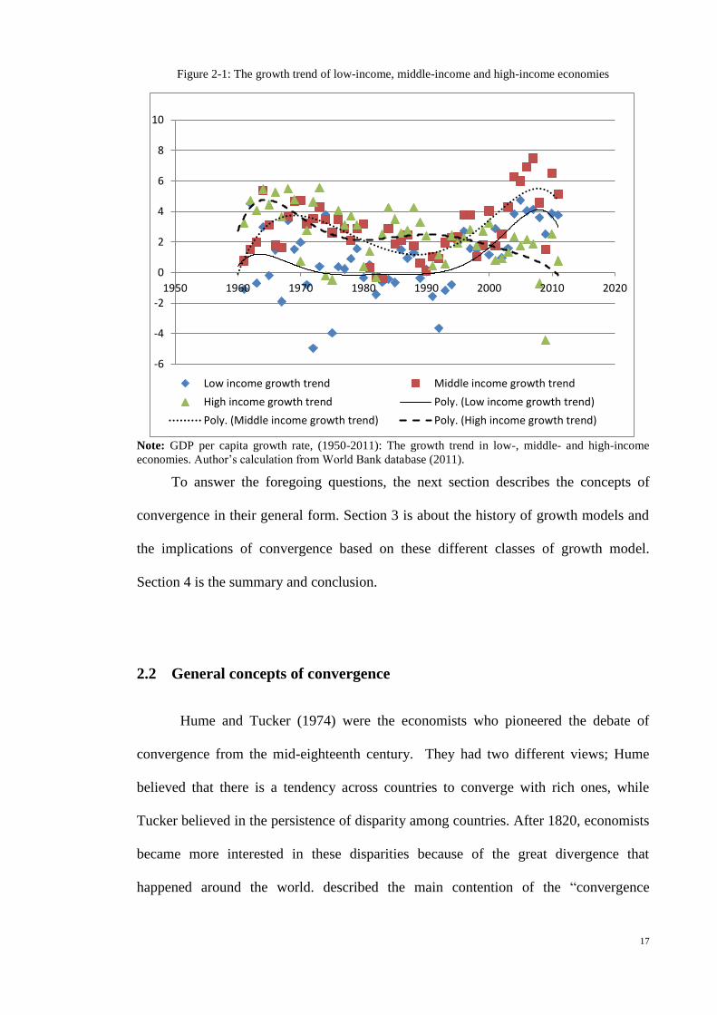
As we can see in figure 2-1, the gap between high-income countries and middle
and low-income countries was at its highest point in the late 1980s, which was not
unexpected because of the oil shock, which happened during 1970, followed by global
recession in the early 1980s. However after this period, the growth rate was boosted,
especially in middle-income countries, and of course, in low-income countries, albeit at
a lower rate, and this growth rate passed even from high-income countries growth rate
in late 1990s. What causes these differences in growth rate across countries to occur? Is
it an automatic force or does it depend on several variables like institutions, the policies
implemented in each economy, their level of human capital and so on? Why could
middle-income countries catch up with the rich ones while low-income countries could
not?
17
Figure 2-1: The growth trend of low-income, middle-income and high-income economies
Note: GDP per capita growth rate, (1950-2011): The growth trend in low-, middle- and high-income
economies. Author’s calculation from World Bank database (2011).
To answer the foregoing questions, the next section describes the concepts of
convergence in their general form. Section 3 is about the history of growth models and
the implications of convergence based on these different classes of growth model.
Section 4 is the summary and conclusion.
2.2 General concepts of convergence
Hume and Tucker (1974) were the economists who pioneered the debate of
convergence from the mid-eighteenth century. They had two different views; Hume
believed that there is a tendency across countries to converge with rich ones, while
Tucker believed in the persistence of disparity among countries. After 1820, economists
became more interested in these disparities because of the great divergence that
happened around the world. described the main contention of the “convergence
-6
-4
-2
0
2
4
6
8
10
1950 1960 1970 1980 1990 2000 2010 2020
Low income growth trend Middle income growth trend
High income growth trend Poly. (Low income growth trend)
Poly. (Middle income growth trend) Poly. (High income growth trend)
18
hypothesis”: ‘Under certain conditions, being behind gives a productivity laggard the
ability to grow faster than the early leader’Krueger and Berg (2003).
Later economists divided the concept of convergence into two categories: Micro
and Macro convergence. R. J. Barro (1991), Rassekh and Thompson (1993), and
O’Rourke, Taylor, and Williamson (1996) defined the concept of micro convergence as
“income of identical factors across countries will equalize based on the factor price
equalization theory under the Heckscher-Ohlin model”. The second concept is macro
convergence, which focused on aggregate factors like per capita income and
productivity. Of course, since these aggregate variables are the weighted average of
factor price, there is a relationship between the micro and macro concepts. The macro
convergence supporters argued that economies tend to converge in terms of per capita
income and productivity over time. These theoretical concepts of convergence need to
be operationally defined:
2.2.1 β Convergence and δ Convergence
There are two concepts of convergence – “β convergence” and “σ convergence”
– which were introduced by R. J. Barro and X. Sala-i-Martin (1995). β convergence
applies when the speed of convergence is faster across poor countries (R. J. Barro & X.
Sala-i-Martin, 1995). Further, they subdivided the “β convergence” concept into
conditional and absolute β convergence. In absolute β-convergence, it assumes that the
only difference in growth rates amongst countries is reliant on their initial levels of
capital. However, in conditional β-convergence some variables are added to the model
to control the differences among economies and, therefore, convergence appear under
some conditions.

19
The other concept is “δ convergence”. If the differences between incomes per
capita of countries decrease over time it indicates δ convergence. One way to test δ
convergence is to measure the standard deviation of GDP per capita amongst countries
over a specific period. If the value of standard deviation in a sample becomes smaller it
means that countries decreased the gap that existed among their income per capita.
Otherwise, there is no convergence.
2.2.2 Club Convergence versus Global Convergence
The other concept is club convergence versus global convergence. The pioneer
who focused on this concept was Baumol (1986), who argued the concept of “club
convergence”. In this concept countries are divided into two groups based on their
growth rate: countries that have lower and countries that have higher growth rates.
Those countries that have middle ranges are going to merge with each of these groups
depending on the rate of the immigrants that they have in each group. Therefore,
countries in each group experience growth or stagnation (Boldrin & Canova, 2001).
Quah (1996), and Ben-David and Papell (1994), in their research also supported the
existence of club convergence.
2.2.3 Income Convergence versus TFP Convergence
The initial studies based on the neoclassical growth models focused more on the
concept of convergence in terms of income, because the important matter in those
classes of models was capital deepening and nothing else. However, with the emergence
of new growth theories, economies started thinking about catching up in terms of
technology, and, since total factor productivity (TFP) was the closest measure for
20
technology, the economies started studying whether or not countries are closing their
gap in terms of the level of TFP.
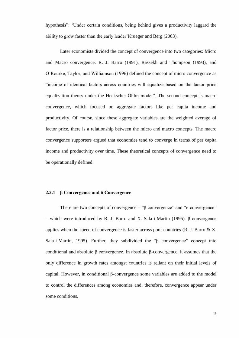
To have a better understanding of the concept of convergence, here we test the
absolute or unconditional convergence in terms of GDP per capita and productivity for
the sample of low-income, middle-income and high-income countries.
Figures 2-2, 2-3 and 2-4 indicate the result of absolute β convergence across
low-income, middle-income and high-income countries, respectively, for the period
1996 and 2010.
Figure 2-2 shows that there is a positive relationship between the growth rate
and initial level of GDP per capita and also productivity across low-income countries
during the period, and, therefore, there is no convergence. However, the slope of fitted
value is sharper in testing convergence in terms of productivity.
Figure 2-2: Convergence across low-income Countries in terms of GDP per
capita and productivity, 1996–2010.
AGO BGDBEN
BFA
BDI
KHM
CMRCAF
TCD
CHN
GMB
GHA
GUY
HIT
IND
IDN
KEN
LBR
MRT
MOZ
NIC
NERNGA
PAK
PNG
PHL
RWA
SEN
SLE
SOM
LKASDN
TGOUGA
TZA
VNM
ZME
-50
510
Gro
wth
rate
of G
DP
pe
r ca
pita
6 8 10 12 14Initial GDP per capita
gdpgr Fitted values
21
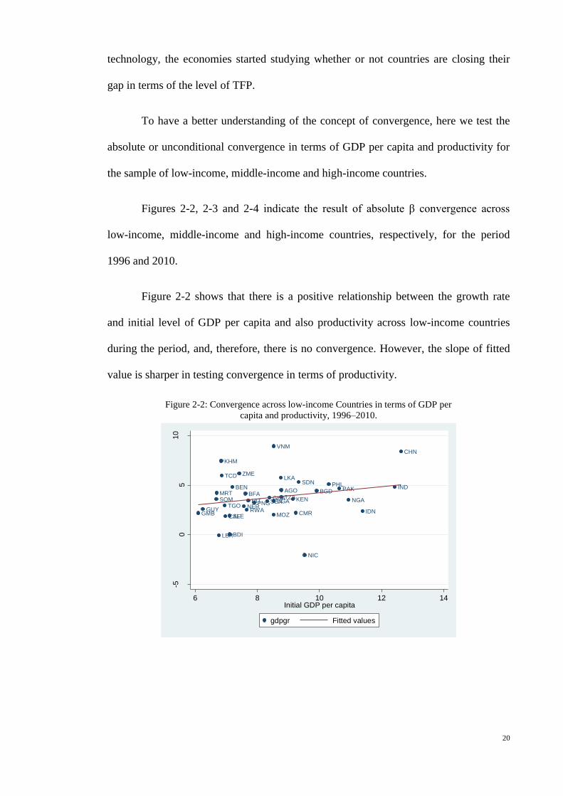
Note: Author’s calculation from World Bank database (2011).
However, in figure 2-3 for middle-income countries, the slope of curves
becomes negative but not that sharp to support absolute convergence. This means that
countries tried to reduce the gap between their incomes.
Figure 2-3: Convergence Middle-income Countries in terms of GDP per capita and productivity, 1996–
2010
BGD
BEN
BFA
BDI
KHM
CAF
TCD COM
ZAR
ERIGMB
GIN
GNB KEN
LBR MDG
MVI
MLI
MOZ
NPLNER RWA
SLE
TZA
TGOUGAZMB
ZMB
-15
-10
-50
5
TF
P g
row
th r
ate
betw
een
199
6 a
nd
200
9
5 10 15 20 25Initial TFP_1996
tfpg Fitted values
Algeria
Bolivia (Plurinational State of)Botswana
Brazil
Colombia
Congo
Costa Rica
Dominica
Ecuador
Egypt
El Salvador
Fiji
Gabon
Guatemala
Honduras Iran (Islamic Republic of)
Jamaica
Jordan
Lebanon
Malaysia
Maldives
Morocco
PeruSamoa
South Africa
Suriname
Swaziland
Syrian Arab Republic
Thailand
Tunisia
Turkey
Vanuatu
12
34
6 8 10 12 14igdp
gdpgr Fitted values

22
Note: Author’s calculation from World Bank database (2011).
Finally, in figure 2-4, the absolute convergence is tested across high-income
countries. As can be seen, there is a strong negative relationship between initial GDP
per capita and the growth rate of GDP, while in terms of productivity it is exactly the
opposite, the relationship is positive. This means that unconditional convergence is not
happening across high-income countries in terms of productivity.
Figure 2-4: Convergence across high-income Countries in terms of GDP per
capita and productivity, 1996–2010
ARGBRA CHL
CHN
CMR
CUB
DJI DZA
ECU EGY
FJI
GAB
IDN
IND
IRN
JOR
LBN
MDV
MEX
MYS
NGA
PAK
SDN
SWZ
SYRTHA
TUNTUR
VENZAF
-4-2
02
4
gro
wth
rate
of T
FP
be
twee
n 1
996 a
nd 2
009
10 20 30 40 50 60Initial TFP96
TFPg Fitted values
AUS
AUT
BEL
CAN
DNK
FIN
FRADEU
GRC
HUN
ISL
IRL
ISR
ITAJPN
KOR
LUX
NLD
NZL
NOR
PRT
ESP
SWE
CHE
GBR
USA
0.5
11.5
8 8.5 9 9.5 10 10.5igdp
grgdp Fitted values

23
Note: Author’s calculation from World Bank database (2011).
Although the convergence hypothesis will be tested in detail in the next chapter,
these graphs help to give a perspective about the convergence hypothesis.
The second concept is δ convergence. Figure 2-5 shows the δ convergence in three
groups of countries.
Figure 2-5: GDP per capita dispersion in the high-income, Middle-income and low-income countries,
1980-2010
Note: Standard deviation of the logarithm of GDP per capita. Author’s calculation from World Bank
database (2011).
AUS
AUT
BEL
CAN
CHE
CZE
DEU
DNK
ESP
FIN
FRA
GBR
GRC
HUN
IRL
ISL ISR
ITA
JPN
LUX
NLDNOR
NZLPOLPRT SVK
SVNSWE
USA
01
23
45
gro
wth
rate
of T
FP
be
twee
n 1
996 a
nd 2
009
60 80 100 120Initial TFP_96
TFPG Fitted values
0.1
0.12
0.14
0.16
0.18
0.2
0.22
0.24
0.26
Middle income
Low income
high income

24
As can be seen, across low-income countries, there is no trend to reduce the gaps
between their incomes per capita; however, across high-income and middle-income
countries δ convergence can be seen.
2.3 Growth Models and Convergence
Since one of the purposes of this study is to compare two models of growth
together, in the next section exogenous and endogenous growth models are defined and
the concepts of convergence based on each model are discussed in detail.
2.3.1 Exogenous Growth Models and the Concept of Convergence
Quantitative growth models have had over half a century of history. In the early
studies, economists believed that physical capital was the main factor for explaining
growth in countries. Harrod (1939) and Domar (1946), for the first time in their famous
model, showed the effect of capital on growth. In their model, society is divided into
two groups: firms and households. The increase in production capacity and aggregate
demand are the two main sources for forming capital. In their model, fluctuation of the
whole production is related to physical capital accumulation. As it is assumed the
capital is rising in proportion to labour; production is carried out in a fixed proportion of
labour and capital. However, an uneven rapid growth rate in some countries showed that
physical capital could not explain the whole fluctuation in growth, which led to the
eventual emergence of neoclassical growth models.
Most of the modern growth models came from the studies done by Solow (1956)
and Swan (1956). In their model, they assumed that there is diminishing return to capital
and labour. The prediction of convergence is derived primarily from this assumption.

25
Constant returns to scale 1 and Inada conditions 2 are other assumptions that they
assumed in their model. While some economists believed that assuming these
assumptions causes the results to be unrealistic, Solow (1956) argued that if the
assumptions that are used in research do not lead to the right results, they are not wrong.
The results showed that policies, which were assumed to be able to change the long-run
growth patterns, could not be effective since they could only affect the short-run growth
rate. The results of their study also asserted that exogenous factors like savings rate,
technological progress and the growth rate of population could affect the growth rate of
an economy (Solow, 1956). Their theory, now referred to as the neoclassical growth
theory, states that, in the long-run, only technological change and population, which are
exogenous, can affect growth (Solow, 1956). Furthermore, in the long-run, economies
are leaning towards zero in their steady state. Therefore, it can be seen that in this
model, the rate of long-run growth is determined totally by exogenous factors and that it
does not depend on other factors like saving rate and policies (R. J. Barro & X. Sala-i-
Martin, 1995).
The steady state for the country is determined by its rate of saving, depreciation
and population growth; if countries have a different steady state, there is no tendency
for convergence among them. Therefore, the only thing that can affect the growth rate in
the long-run, as said before, is the rate of exogenous technological progress.
Hence, according to the neoclassic growth theory, two equations are important
in analysing growth: production function equation (2-1) and accumulation equation (2-
5). The factors in Cobb-Douglas production function can be summarized into two items:
physical capital K (t) and effectiveness of labour𝐴𝑡𝐿𝑡 . Then the production function
takes the form as below:
1 -“ A production function exhibits constant returns to scale if changing all inputs by a positive proportional factor has the effect of
increasing outputs by that factor.” 2 - “are assumptions about the shape of a production function that guarantee the stability of an economic growth path in a
neoclassical growth model”
26
𝑌𝑡 = 𝐾𝑡 ∝(𝐴𝑡𝐿𝑡)1−∝ 0<α<1 (2-1)
Where 𝑌𝑡 is output, Kt is physical capital, At is technology, Lt is labour, α is capital
share so there is diminishing return to capital. L and A assumes growth at an exogenous
rate according to the following functions:
𝐿𝑡 = 𝐿0𝑒𝑛𝑡 (Simply normalize 𝐿0 to unity) (2-2)
𝐴𝑡 = 𝐴0𝑒𝑔𝑡 (2-3)
Considering the constant return to scale assumption, the intensive form of production
function is as follows:
𝑦�� = ��𝑡𝛼 (2-4)
Where, ��=K/AL and ��=Y/AL. One of the assumptions in the neoclassical model is to
consider that the economy is closed. Therefore, when a country reaches to its steady
state, equilibrium happens and so saving and investment would be equal. Therefore, a
change in capital during time is determined by the following equation (accumulation
equation):
𝑘�� = 𝑠��𝑡𝛼 − (δ+ g + n)��𝑡 (2-5)
Where s is saving rate, δ is the depreciation rate of capital, n is the constant growth rate
of the population and g is the growth rate of technology (R. Barro & Sala-i-Martin,
2004)
In the steady state the accumulation of capital is constant; therefore, we have:
𝑘∗ = [𝑠
(𝑛+𝑔+𝛿)]1/(1−𝛼) (2-6)
Insert this equation into (2-4), the equilibrium effective per output equation is as
follows:
𝑦∗ = (𝑠
(𝑛+𝑔+𝛿))
𝛼1−𝛼⁄ (2-7)
Taking logarithm from equation (2-7):
ln(𝑦∗) =𝛼
1−𝛼ln 𝑠 −
𝛼
1−𝛼ln(𝑛 + 𝑔 + 𝛿) (2-8)

27
Since there are no data for the effective per income equation, the equation should be
transferred back to a per capita income form. We had �� = Y/AL, therefore, by taking
logarithm, we have:
Ln(��) = Ln(Y) - Ln (L) – Ln (A) (2-9)
=Ln(y) - Ln (A) (2-10)
Then taking logarithm from equation (2-3) and substituting it in equation (2-10),
Ln(��)= Ln(y)- Ln(𝐴0) – gt (2-11)
And, finally, we have:
ln[𝑦∗] = 𝑙𝑛𝐴0 + 𝑔𝑡 +𝛼
1−𝛼ln(𝑠) − ln (𝑛 + 𝑔 + 𝛿) (2-12)
This equation is for the level of per capita income, Where 𝐴0 reflects country specific
factors, such as climate and culture (N. G. Mankiw et al., 1992). For deriving a model
for growth of income per capita, we linearize the transition growth path, and we assume
the country is sufficiently close to its steady state so linearization is appropriate.
𝑑𝐿𝑛𝑦��
𝑑𝑡= 𝜆( 𝐿𝑛��∗ − 𝑙𝑛��𝑡) (2-13)
Where 𝜆 = (𝑛 + 𝑔 + 𝛿)(1 − 𝛼) is speed of convergence. Now we want an equation to
treat it like a regression equation. We integrate equation (2-13) from yt to y0:
Ln( ��𝑡 ) = (1 − 𝑒−𝜆𝑡)𝐿𝑛(��∗) + (𝑒−𝜆𝑡) ln ��0 (2-14)
Where ��∗is the steady state for output per effective worker and let 𝑦𝑜 be the initial level
of output, therefore, we have to transfer it to the format of per worker by using equation
(2-11). Therefore, we have:
𝐿𝑛 𝑦𝑡 − 𝑙𝑛𝑦0 = (1 − 𝑒−𝜆𝑡)𝑔 + (1 − 𝑒−𝜆𝑡)ln (𝐴0) + (1 − 𝑒−𝜆𝑡)𝐿𝑛(𝑦∗) + (𝑒−𝜆𝑡) ln 𝑦0
(2-15)
And by substituting 𝐿𝑛(𝑦∗) by its amount in equation (2-15):
Ln( 𝑦𝑡 – 𝑦0) = (1 − 𝑒−𝜆𝑡)𝑔 + (1 − 𝑒−𝜆𝑡)ln (𝐴0) + (1 − 𝑒−𝜆𝑡)𝛼
1−𝛼𝐿𝑛(𝑠) +
(1 − 𝑒−𝜆𝑡)𝛼
1−𝛼𝐿𝑛(𝑛 + 𝑔 + 𝛿) − (1 − 𝑒−𝜆𝑡) ln 𝑦0 (2-16)
28
A more general form of equation, which is used in empirical panel studies, is:
Ln( 𝑦𝑡,𝑖 – 𝑦𝑖,𝑡−1) = 𝛽1𝐿𝑛(𝑠𝑖,𝑡) + 𝛽2𝐿𝑛(𝑛𝑖,𝑡 + 𝑔 + 𝛿) − 𝛾 ln 𝑦𝑖,𝑡−1 + 휀𝑖,𝑡 + 𝜇𝑖 +
𝜑𝑡 (2-17)
Where 𝜇𝑖 and 𝜑𝑡 are time specific and country specific effects and β1, β2 and γ
are parameters to be estimated. By equation (2-17), which is from the Solow-Swan
model, the link between the growth model and convergence becomes clear. As we can
see the speed of convergence ( 𝛾) is dependent on the initial level of income and the
structural parameter of neoclassical growth model, which is what economists like R. J.
Barro and X. Sala-i-Martin (1995), and N. G. Mankiw et al. (1992) called conditional
convergence. When an economy starts with a level of capital per unit of effective labour
lower than the steady state, the level of capital monotonically increases to its steady-
state value. This means that the growth rate decreases monotonically. Since output
varies with the capital, the growth rate of production also declines monotonically when
the level is below its steady state level. In other words, poor countries grow faster than
rich countries, on the assumption that both have the same technologies and preferences,
until they converge to the same steady state.
2.3.2 Endogenous Growth Models and the Concept of Convergence
For the period after World War II, empirical studies showed that the neoclassical
model is incapable of explaining the differences across growth rates of countries.
Economists believed that by taking technological progress as an endogenous factor,
each country’s growth rate can be determined. Therefore, attempts to endogenize
technology started. The only problem that this class of model faced was about the
assumption of increasing return in a general equilibrium framework rather than
decreasing return, which was the fundamental assumption of the neoclassical model. In

29
other words, according to the Walrasian theory of general equilibrium, all factors must
be paid their marginal products. However, according to the Euler theory on assuming
increasing return, all factors cannot be paid their marginal products. Therefore,
something beyond the Walrasian theory should be found.
Arrow (1962) made the initial study that tried to endogenize technology into the
growth models. He assumed that the growth rate of technological progress is a result of
commodities produced by labour based on their experience. In other words, the
technology can be affected by “learning by doing”. This means that labour productivity
is endogenous. The important point here, in this model, is to assume that the learning
factor is free for all firms, with no cost, like public commodity. The problem with
Arrow’s model was that the model only works when the ratio for capital-labour is fixed.
That means in the long-run the growth rate is limited to labour growth rate, and,
therefore, the saving rate does not play a role and the model is not dependent on saving
behaviour, like the Solow model.
Another person who tried to endogenize technology was Nordhaus (1969), who
made an assumption of an economy based on the neoclassical framework except for
knowledge production. Capital and labour produce output through an aggregate
production function. What makes his model different from the previous ones is that it
integrates an invention factor into the economic analysis. In general, invention means
the activities that can expand the level of technology. As opposed to the “Schumpeter
tradition”, which believed that invention is an exogenous factor in an economy,
Nordhaus (1969) believed that there is a relationship between invention and economic
activities. He equated the rate of technology as an increasing function of the number of
innovations produced, and, therefore, he endogenized technology in his model. He
generated some new twists for the new model of invention. He took invention as a

30
variable that is produced in the system as a new production process. Invention is
regarded as a public commodity and available for any firm without costs. In practice,
the inventor can keep his invention as a secret for a specific period of time but after this
period, his monopoly is relinquished and it is free to be used by any other firm.
However, in the Nordhaus model, just as Arrow’s model, the growth rate cannot be
sustained without accounting for population growth because of the assumption of
increasing returns. Economists like Hicks (1963) also introduced “invention possibility
set” models and Kennedy (1964), Samuelson (1965) and von Weizsäcker (1966)
followed suit and fully collaborated their findings. Uzawa (1965) studied the “optimal
education” model and emphasized the role of an educated labour force as an input in the
production function, and analysed the optimal growth path. However, all these models
faced the problem of increasing return. They could not answer the question of how the
economy would compensate activities to make technology grow when there is an
increase in returns and endogeneity of technology.
2.3.2.1 First Generation of Endogenous Growth Models
According to the neoclassical growth model, technological progress is an
exogenous factor and is the only factor that can permanently affect growth rate in the
long-run, while other permanent shocks like change in human capital; saving rate and
population have a temporary effect on growth. However, P.M. Romer (1986) argued
that this assumption is not reliable since it does not explain how or why technological
progress occurs. Therefore, to answer these questions of new growth theories,
endogenous growth models were introduced. P.M. Romer (1986) lumped physical
capital from saving and intellectual capital from technology together, therefore it can
offset the effect of diminishing returns. In these models technological progress is an

31
endogenous factor of economic growth and the heart of growth that is determined by the
growth process through the accumulation of workers employed in knowledge-producing
activities. In other words, growth is explained by technological progress and
technological progress is the outcome of optimizing firms and individuals undertaking
investigation in R&D and schooling. The production function of ideas is the source of
growth. The parameters in the idea production function show whether innovation
through R&D can affect growth permanently or temporary. As can be seen, in the
endogenous theory, the role of human capital is important since it is a source of
knowledge and knowledge is directly related to technological progress. Furthermore,
human capital is a source for creating different new products and is also the only source
that can inherit knowledge from past generations. In the endogenous growth models the
long-run growth is accrued because of the accumulation of knowledge. Knowledge, as
P. Romer (1991) said, is a basic form of capital, which changes the nature of the
aggregate growth model. He believed that “an economy with a large total stock of
human capital will experience faster growth”. Therefore, he explained that growth is not
happening in underdeveloped countries, because of the low level of human capital and
that less developed countries have less growth because of their large population. In
these models, there is a positive relationship between the level of R&D and productivity
growth(P. Aghion & Howitt, 1997; P. Romer, 1991). An increase in the size of
population will increase researchers in the R&D sector, which increases activities, and,
ultimately, increases productivity.
The important point in these new models is the role of increasing returns as
opposed to diminishing returns in neoclassic models. Knowledge and other inputs, as a
function of production of goods, have increasing marginal product. The presence of
externalities and increasing returns in producing new knowledge introduce a very
competitive equilibrium growth model. The existence of equilibrium is dependent on

32
the externalities. Even without the condition of increasing returns, equilibrium will
coexist with externalities. The increasing return to knowledge is necessary to ensure that
the consumption and utility do not grow too fast. The important item here, which makes
this model different from the older one is the assumption of increasing marginal
productivity of the intangible capital good knowledge (P.M. Romer, 1986)
P.M. Romer (1986), in his study, following the Maddison database 1979
(Maddison, 1979) for emphasizing the role of knowledge, showed that there is no
relationship between the initial income per capita and the growth rate of a country. He
indicated that output per person has increasing returns relative to the growth rate of the
technology leader. He believed that technology came from innovation and innovation is
directly related to the rate of scientific progress. In addition, economic activities and
decisions can also affect technological progress. For example, one of the factors that can
affect technological progress is research and the development sector, which occurs
through economic policies that can affect competition, trade and education. He selected
eleven industrialized countries and showed that the growth rates of these countries are
higher than the previous decade by 0.85 for Sweden and 0.81 for Norway. Furthermore,
in 22 developed economies he found a positive relationship between the growth rate of
output and the number of scientists and engineers who are employed in research. Today,
his approach is known as the AK model. The simplest form of AK model mentioned is
the Cobb-Douglass production function:
𝑌 = 𝐴𝐾𝛼𝐿1−𝛼 (2-18)
In the AK model, α is equal to one, therefore, the equation is remodelled to this form:
Y=AK (2-19)
33
Where A represents the level of technology, which is a positive amount, and, here, K
includes human and physical capital. Therefore, this makes the absence of diminishing
returns more realistic. As said before, in the neoclassical model the fundamental
equation is as follows, which depends solely on K:
�� = 𝑠. 𝑓(𝑘) − (𝑛 + δ). 𝐾 (2-20)
The growth rate of k is driven by division of both sides by k:
��𝑘
⁄ = 𝑠.𝑓(𝑘)
𝑘− (𝑛 + δ) (2-21)
By substituting f (k)/k= A in equation (2-21), then the following equation results in:
F (k)/k=s.A-(n+δ) (2-22)
This shows the growth rate of K. This equation shows that growth can happen
even without technological change. Moreover, growth is not only dependent on
technological change, but can also be affected by parameters in the model like the
savings rate and population growth. Except for diminishing returns, this is one of the
main differences between the neoclassical models and endogenous ones.
The other difference concerns the prediction of convergence; in the endogenous growth
models of P.M. Romer (1986), there is no convergence at all at any level of y, which is
contrary to what neo-classical models predicted about convergence. As said by Solow
(1956), “the speed of convergence is determined by:
λ= (1 -α). (g+ n +δ) (2-23)
In the AK models α=1, the share of capital in the Cobb-Douglas function, therefore,
when λ is equal to zero, it means that there is no convergence, and it does not matter
whether the country is poor or rich.

34
After P.M. Romer (1986), Lucas (1988) was another economist who had a
significant effect on endogenous growth models. The model that Lucas developed was
a two-sector model that emphasized the role of education on growth, assuming that
population growth and all the other factors were endogenous. He divided capital into
two categories: one is physical capital that is accumulated in production and produced
by the technology of consumption good and the other kind of capital is human capital
that increases productivity on its own and is produced by a different technology. Human
capital here has increasing marginal returns and creates endogenous growth. He
believed that a labour force with high education is able to learn faster than one without
high education. The importance of human capital came from the idea that the formation
of the next generation of human capital is affected by earlier generations. He believed
that every unit of human capital produces new units of human capital. Lucas believed
that human capital has a positive effect on growth. In his model, the first sector is for
the production of output and the second sector is for the production of new human
capital. Therefore, if one ignores the positive external effects of human capital,
endogenous growth can only be possible if there are constant or increasing marginal
returns to human capital accumulation. This model, just as Romer’s model (1986),
predicts no convergence and there is no decline in the growth rate of developed
countries. Economists like Scott (1991) supported this idea and showed that there has
been no tendency of a decline in the productivity growth rate in the US, United
Kingdom and Japan in the last thirty years.
During the second half of the twentieth century, some empirical studies
indicated that some countries have been converging to the same steady state; however,
these results were not consistent with the first generation of endogenous theory in which
there is no convergence for countries in terms of GDP per capita. In 1992, Mankiw,
Romer and Weil (henceforth MRW) reconsidered the Solovian production function and
35
argued that it is not necessary to rely on the endogenous models to explain the
divergence across countries. As explained before, λ is the speed of convergence in the
Solow model: λ= (1 -α). (g+ n +δ). As we can see here, the share of capital α, which is
highlighted in the assumption of diminishing returns, is very important in determining
the speed of convergence. The Solow model explains that a smaller α, leads to faster
convergence. As it becomes equal to zero the diminishing return disappears and there
will be no convergence. The contribution of MRW to the literature here, is that they
augmented human capital to the model in addition to physical capital and argued that if
we consider the process towards steady state transitional dynamics, as protracted, the
Solow model could explain the different growth rates across countries. By augmenting
human capital to the model the income elasticity becomes 1 rather than ½ in the Solow
model and the performance of the model improves. Furthermore, they obtained an
expression for the steady state of income per capita:
ln(𝑦��) = 𝑙𝑛𝐴(0) + 𝑔𝑡 +𝛼
1−𝛼−𝛽𝑙𝑛𝑠𝑘 +
𝛽
1−𝛼−𝛽𝑙𝑛𝑠ℎ −
𝛼+𝛽
1−𝛼−𝛽ln (𝑛 + 𝑔 + 𝛿) (2-24)
Equation (2-24) shows that the steady state level of income per capita is
positively related to A(0), which, according to MRW, is not just the level of technology
but also other variables like culture, institutions and climate. Furthermore, more
importantly, it is related to the rate of accumulation of human capital in addition to other
Solow factors. In their analysis, they let the population growth rate, saving rate and
secondary school enrolment change across countries and determine the steady state. By
doing so, they found evidence of convergence even in a big sample of countries with
different structures. The MRW model is influential in the growth-convergence debate
for two reasons. First, they augmented human capital as an additional controlling
variable for steady state. Second, the empirical evidence of their model considered
convergence, which was rejected by the first generation of endogenous growth models.

36
Evans and Karras (1996) also showed that the Solow-Swan (1956) models could
explain the growth rate of countries with common technology around the world. In
addition, R. J. Barro and X. Sala-i-Martin (1995), in their studies, indicated that
convergence happened based on the neoclassical models but not endogenous ones.
These findings had a double impact, on the one hand, some economists think that the
Solow model could explain the convergence progress across countries and are working
to extend the model and test it with new controlling variables and updated time series
and methods. On the other hand, these findings pushed economists to study more about
technological advances and pay more attention to the role of innovation, which was
used by Schumpeter years before and led them to a new aspect of growth theory.
2.3.2.2 Second generation of endogenous growth models
In 1995, C. Jones (1998), in his book, argued that the “scale effect” predictions
of many recent ideas for production functions (P. Aghion & Howitt, 1997; P. Romer,
1991) are not consistent with empirical evidence. For example, in the case of the US,
between 1950 and 1990, the number of researchers was five times bigger than before
but still the growth rate was 2 per cent. Therefore, the prediction “constant return to
knowledge” of these models was not consistent with the empirical evidence. However,
this inconsistency does not refute the important role of R&D based growth models.
Therefore, in the other generation of growth models the researchers eliminate this fact
and retain the other features of R&D based models. In addition, semi endogenous
growth models were introduced. In these models, they relaxed the assumption of
constant or increasing return to knowledge and substituted diminishing return to
knowledge. Therefore, for a sustained growth rate, growth in R&D is required. Kortum
(1998) and P. Aghion and Howitt (1997) supported these ideas. On the one hand, this

37
class of model was similar to Romer’s, in which growth drives endogenously through
R&D, while, on the other hand, it is similar to the Solow model in which long-run
growth only depends on those factors that are usually exogenous, especially population
growth rate, which could be a proxy for innovators and scientists, and, therefore, is
independent of policy changes in economies.
Considering the following Cobb-Douglas production function (J Ha & P Howitt, 2007):
𝑌 = 𝐴𝐾𝛼𝐿1−𝛼 (2-25)
Where Y is output, A is level of technology, K is capital stock, L is labour force and α is
capital share, which is assumed to be constant. The growth in ideas production function
for the first generation of endogenous growth models is given by:
��
𝐴= 𝛾(𝑋)𝜎 (2-26)
Where �� is the number of new ideas generated, A is the stock of knowledge, γ is
the research productivity parameter, X is R&D input and σ is the duplication parameter
(1 if there are no duplication innovations and 0 if there are a number of innovations). In
the first generation of endogenous models, they assumed a constant return to
knowledge, and, therefore, that policies that determine R&D input will affect the long-
run growth rate. The failure of this model is the back to scale effect item, which states
that the higher the level of R&D input, the higher the productivity growth.
As mentioned above, C. Jones (1998) refuted this theory and introduced the semi
endogenous growth model, as follows:
��
𝐴= 𝛾(𝑋)𝜎 𝐴𝜃−1 , θ<1 (2-27)
Where, θ is return to scale in knowledge, which is diminishing here. Therefore, this
model assumes that there is a positive relationship between R&D growth and
productivity growth.

38
P. Aghion and Howitt (1997) wrote a paper in response to Jones’ critique. In
their paper, they argued that having sustainable productivity growth in an economy
requires a sustained R&D intensity, and the size of the labour force (GDP) employed
(spent) in the R&D sector rather than growth in R&D (Dinopoulos, 2006; J. Ha & P.
Howitt, 2007; Madsen, 2008).
A
A= γ(
X
Q)σ Aθ−1 , Q ∝ Lφ , θ<1 and 0 < θ ≤ 1 (2-28)
Where, Q is product variety, L is employment or population and φ is the
parameter of proliferation and X
Q is research intensity. This equation implies that the
increasing rate of population will increase the number of people who can innovate new
products. The difference between this model and previous ones concerns the
assumptions of increasing complexity of innovation, which enter R&D as research
intensity instead of just R&D input.
They assumed a constant return to scale like the first generation; however, they
added a new assumption – increasing complexity of new innovation. These models are
famous as the Schumpeterian fully endogenous growth models. They called them
Schumpeterian fully endogenous growth models because they were inspired by the
theory of “creative destruction” which was introduced by Schumpeter:
“The process whereby each innovation creates some new technological
knowledge that advances our material possibilities, while rendering obsolete some
of the technological knowledge that was created by previous innovations”(Howitt,
2000).
In these models, physical capital and intellectual capital were separate and saving
is the result of former growth and later growth is from innovation (P. Aghion & P.
Howitt, 2006). Here, growth is the reason for the innovation process that improves the
39
quality of outputs, which is inspired by “research activities with uncertain results”. New
inventions render previous technologies obsolete; this is called “the factor of
obsolescence”, which is the embodiment of Schumpeter’s idea of “creative destructive”.
The “creative destructive” progress pointed out two conflicting aspects of research
activity. On the one hand, researchers in this period will develop research and new
inventions in the next period, and, on the other hand, new inventions and research
render the previous ones obsolete. Furthermore, if the research that firms have done is
successful, they can have the monopoly of that patent (P. Aghion & P. Howitt, 2006). It
is clear that in this class of models, the role of R&D is very important, and, as J. Ha and
P. Howitt (2007), and Madsen (2008) pointed out, if a country wants to have sustainable
productivity growth, more labour force (GDP) should be employed in the R&D sector.
Howitt (2000), based on the fully Schumpeterian endogenous growth models, suggested
that those countries that attempt to increase their R&D sector will reduce the gap with
rich countries and will increase their growth while those that do not will not grow at all.
The growth rate of productivity is determined by multiplying the research intensity with
the technological gap between a country and a country in the technology frontier.
Countries that are further from the frontier will grow faster in this model.
A
A= τ (
X
Q) (
A𝑀𝑎𝑥−𝐴𝑡
𝐴𝑡) (2-29)
Where τ is the R&D productivity parameter, X
Q is the research intensity and A𝑀𝑎𝑥
is the country in the frontier. If A𝑀𝑎𝑥 remains at the same level and the research
intensity increases, the countries lying behind can converge to the leader’s level of
productivity. Nelson and Phelps (1966) argued that human capital plays an important
role in absorbing foreign technology. They added the human capital time technology
frontier to the model and named it “theoretical level of technology, T”, and showed that
improvement in technology is not only dependent on human capital but also on the gap
40
between the level of theoretical technology and technology in practice. In their model,
similar to the Solow model, the long-run growth rate of technical progress is still
exogenous.
A
A= ω(𝐻𝐶)(
𝑇𝑡−𝐴𝑡
𝐴𝑡) (2-30)
In other words, according to this equation, the technological gap will be dependent on
the level of human capital (Raiser et al., 2001).
R. Griffith, Redding, and Reenen (2004) employed a model, which tested the
two faces of R&D: one is the effects of R&D on innovation and the other is the effect of
R&D on absorptive capacity and promoting convergence. This model implies that R&D
is not just promoting TFP growth but also helps technology transfer across countries:
A
A= γ (
X
Q) + 𝛽 (
A𝑀𝑎𝑥
𝐴𝑡) + 𝛼 (
X
Q) (
A𝑀𝑎𝑥
𝐴𝑡) (2-31)
The third term on the right shows the effect of research intensity based on absorptive
capacity.
From equation (2-31), the link between TFP growth and distance to technology
frontier can be seen. The sign of β shows whether or not catching up happened across
countries, if it is positive it means that countries are catching up to advanced economies.
Since technology is very important for growth, especially in this class of model,
knowing the channels for innovating new technologies and also the channels through
which these technologies can be transferred to other countries is very important.
Therefore, innovation and imitation play an important role in the catching up process.
This research tries to focus on this part and contribute to literature by looking through
different channels for transferring technology across countries. In the next section the
history of growth theories will be discussed to see how different classes of growth
model have been created and how they deal with the convergence issue and also
technology and other important factors as sources of growth.

41
Later, R Griffith, Redding, and Van Reenen (2004) extended the model of P
Aghion and Howitt (1998) by focusing more on the role of R&D as an accelerator of
absorptive capacity and incorporated it in the Schumpeterian fully endogenous model.
They were inspired by the idea of P Aghion and Howitt (1998), who introduced income
convergence by “allowing the size of the quality-augmenting innovation to depend on a
firm’s distance behind the technological frontier” (R Griffith et al., 2004) (R Griffith et
al., 2004) (R Griffith et al., 2004) (R Griffith et al., 2004) (R Griffith et al., 2004) . In
these models, the rate of technological progress depends on research and countries can
benefit from the backwardness in their technology and grow faster. Therefore,
according to this backwardness these recent models also cover the convergence debate
through technology transfer (R Griffith et al., 2004). R Griffith et al. (2004), in their
paper, extended the P Aghion and Howitt (1998) model and emphasized three parts –
R&D based innovation, the potential for technology transfer and the role of R&D in
promoting absorptive capacity. They argued that countries further from the technology
frontier can grow because of both innovation and technology transfer. The important
point in their paper is that if the research is not successful in the first period the
technology can transfer independent from R&D activities. They called it “autonomous
technology transfer”. In addition, they emphasized that the pace of this transfer is a
function of government policies, institutions, international trade, and level of human
capital. In other words they captured the role of R&D as a promoter of absorptive
capacity and not just innovation. More investment in the R&D sector and more foreign
technology could be absorbed and the important thing here is that developing countries
should not only focus on importing technology from developed countries but also work
on their own domestic technological activities (Fagerberg, 1994). Therefore, a country
that is far from the technology frontier has more benefit and can grow faster considering
42
the role of human capital, trade, institutions as well as investment in R&D. The
following equation (2-32) was employed by R Griffith et al. (2004):
(2-32)
Where E is an “expectations operator”. This equation is inspired from
Schumpeterian endogenous growth. Innovation is the main factor in determining
economic growth. This equation also includes empirical evidence of productivity
convergence. The potential of transferring technology denotes that those countries far
from the frontier ( ), can experience a faster growth rate than the others.
Although all of the countries that are away from the technology frontier have this
potential to grow, the possibility of this event depends on the institutions and
government policies ( μi ) and the absorptive capacity of countries. With more
investment in the research and development sector, the ability of a country to assimilate
from new technology will be increased, and, therefore; it can increase the rate of
technology transfer.
According to this equation, the equilibrium level of relative TFP depends on the
following factors:
Institutions and government policies, which affect research productivity (λf, λi).
Size of labour force that works in the research sector ( , ).
The size of innovation, which is at the technology frontier (δ).
Political-economic variables, which form the speed of abstractive capacity
during technology transfer (φi , µi).
1 1 1 1 11 1 1
1 1 1 1 1 1
ˆ ˆR Ri t f t f tt i it i i it i
i t i t i t
A A AE Ln H Ln Ln H Ln
A A A
1 1 1 1i t f tA A
ˆ R
fH ˆ R
iH

43
Now we can see the concept of convergence through these models. The further a
country is from the technology leader, the greater the productivity growth it could have.
This is the concept of convergence in the Schumpeterian fully endogenous growth
models. In our study, we were inspired by the Schumpeterian fully endogenous growth
theory to drive our productivity regression.
2.4 Summary
The question about income inequality across countries has been an important
question since 1820, when the great divergence happened in the world. Since then,
economists have tried to explain this disparity by employing different theories, models
and methods. In previous studies economic indicators like saving, investment, capital,
trade, foreign direct investment (FDI) and socioeconomic indicators like education and
health have been used to explore the different growth across countries. However, the
uneven growth disparities across countries make it difficult to conclude which factors
are more effective. In addition, in the new growth theories the concept of technological
catch up came into sharp focus. Technologies have always been an engine of growth in
all growth theories. In the neoclassical theory, they treat it as an exogenous factor;
however, in the new growth model it is endogenous, which is determined inside the
model. While in previous studies most researchers focused on the concept of
convergence in terms of GDP per capita (or β convergence), recent studies supported
that a large fraction of income disparities can be explained by technological change (or
total factor productivity, TFP). They argued that income convergence can be the
outcome of both capital deepening and technological catch up. Therefore, economists
directed their attention to this concept (Charles Jones, 1998; Madsen, 2008; Raiser et
al., 2001). Since TFP is the closest measure for technology, researchers use it for

44
investigating whether or not countries are closing their gap in terms of their TPF levels.
In this debate, the distance to the technology leader is very important. The further from
the technology leader the country, the more advantage it has from this backwardness
and grows faster. Therefore, we can see that the concept of convergence here changes
from the distance from steady state to distance from technology frontier.
In this section we described the different growth models and compared them, and
described the theoretical framework of these models, making clear the link between the
growth models and convergence hypothesis, which is how we can test the convergence
hypothesis through these models. Also, we described the different concepts of
convergence that exist in the literature, absolute β convergence and σ convergence in
terms of GDP per capita and technology catch up in terms of TFP.

45
3 Chapter 3
Reopening the Debate of Technology: Innovation and Imitation
Perspective, Empirical Framework
3.1 Introduction
Looking back through history we can see that the role of technology became very
important during World War I and II, and even more important after the emergence of
three tigers in Asia (Singapore, Thailand and Korea). Economists have conducted a lot
of research to understand what is going on and tried to explain this massive growth rate
through different channels. A large portion of literature in this field investigated the role
of technology and how it can affect growth in different countries. However, most of the
studies in this field are radical and stick to the school of thought that they believed. For
example, the neoclassical people try to prove that capital accumulation is the main
source of growth without considering the role of technology. They believed that
technology is important but they did not try to look at the role of imitation and
innovation of technology through the accumulation of capital in their model.
Furthermore, in the new growth theory they considered the role of imitation and
innovation in their model but they ignored other items like the role of institutions and
globalization as factors that could increase the pace of imitation, and, consequently,
increase the growth rate of countries.
Therefore, this research tries to reopen the role of technology in these two classes
of model by focusing on the role of imitation and innovation.
46
3.2 Reopening the Debate of Technology
Although technology is assumed to be a main source of growth in all kinds of
growth model, it can affect growth through different channels in each class of model.
Neoclassic economists argue that technology is a public good and the same across
countries, and, therefore, the rate is constant and exogenous, while in the endogenous
theory they argue that it is not the same across countries and that the rate is endogenous
and determined inside the model. Therefore, the debate of how it should be endogenized
in the model remains an interesting topic.
At the same time, the disagreement between neoclassic people and new growth,
make this debate more interesting. Researchers have conducted empirical studies using
these different theories with different methods, which have contributed considerably to
this area.
Such studies include those done by N. G. Mankiw et al. (1992) who introduced
the augmented Solow model, separating human capital from physical capital, or Charles
Jones (1998), who introduced the semi endogenous models by emphasizing R&D
activities or P. Aghion and Howitt (1997), who introduced the fully endogenous growth
models, which is also famous as the technology-gap models that emphasize the role of
R&D intensity and absorptive capacity. In recent attempts, economists focussed more
on the role of innovation and imitation on these models and tried to endogenize them
into growth regressions (Phelps, 1966; J. D. Sachs, 2003). The more investment, for
example, in R&D departments, causes more innovation, which has a direct effect on
increasing productivity and growth. Furthermore, increasing the ability of the country to
imitate these new innovations from the other countries can also increase the productivity
and growth. These two aspects are seen to be very important in explaining the growth
rate across countries.

47
However, in considering the role of two factors – institutions and globalization –
that appear to have been ignored, we shall contribute to the analytical literature by
discussing their role as accelerators of absorptive capacity as well as the role of human
capital, which has been extensively discussed. We shall derive the technology-gap
regression taking into account these new variables. Furthermore, to show how these
different dimensions of technology evolved in past years, this study follows the standard
analysis of testing β and σ convergence. Finally, to link the technological change to
convergence in terms of income we estimate the classic growth regression, which
decomposes GDP per capita growth into the sum of dynamic of technology change and
physical capital accumulation rate. Section two extends the Solow model by including
these new aspects of growth, which are highlighted in the new growth theories. In line
with the augmented Solow model, this study applies globalization and institutions as
well as innovation as factors that increase the accumulation of human capital, and drives
a regression, which can be tested empirically.
3.3 Reopening the Debate of the Knowledge Transfer on NGM
New growth models are different from NCGM in that knowledge is a key source
of growth. The stock of knowledge plays an important role in explaining the different
growth rates across countries. Therefore, the components of knowledge stock are very
important. Creation (CKi) and imitation (IKi) are two components of knowledge stock
growth that have attracted considerable attention in recent growth literature (Castellacci,
2011).
∆𝐴𝑖
𝐴𝑖= 𝐶𝐾𝑖 + 𝐼𝐾𝑖 (3-1)

48
Technology (knowledge) spillovers or imitation is considered as an important
item in explaining growth. Hitherto, in most of the existing models, technology transfer
was considered as an automatic phenomenon, and none of the models could explain
through which mechanism technology transfer happens across countries and affects
growth. Therefore, factors that can be considered for imitating and implementing new
technologies from advanced countries are becoming very interesting in empirical
studies. Imitation depends on the distance to technology frontier (DTFi), in which
countries that lie behind the technology frontier have the opportunity to catch up by
imitating technology from leaders, and absorptive capacity (ACi), which shows to what
extent countries have the ability to absorb technology from frontiers (Beck & Laeven,
2006; Jess Benhabib & Rustichini, 1996; R. Griffith et al., 2004; R. R. Nelson, 2008;
Phelps, 1966; Pomeranz, 2001; Raiser et al., 2001; J.D. Sachs, 2003).
𝐾𝐼𝑖 = 𝐷𝑇𝐹𝑖𝜇 ∗ 𝐴𝐶𝑖 (3-2)
In previous studies, the absorptive capacity depends on R&D (R. Griffith et al.,
2004) and human capital (HCi) (D. Dollar & Kraay, 2004; Madsen, 2008), and, by the
study done by Castellacci (2011), it is a function of human capital and infrastructure. In
this study, we argue that institutions (INSi) and globalization (GLOBi) are the other
factors that can improve the ability of a country to observe foreign advanced
technologies. Without having proper institutions (e.g. property rights) in a country,
inventors do not innovate, and, therefore, there is no knowledge to transfer across
borders. The other factor is globalization (GLOBi), which can improve the absorptive
capacity. Flow of ideas, as well as flow of goods, are very important in accelerating
growth. Therefore, human capital would be useless without the support of proper
institutions and the existence of globalization in terms of ideas.
𝐴𝐶𝑖 = 𝐻𝐶𝑖𝛽1 ∗ 𝐼𝑁𝑆𝑖
𝛽2 ∗ 𝐺𝐿𝑂𝐵𝑖𝛽3𝑅&𝐷𝑖
𝛽4 (3-3)
49
The other component is creation of knowledge (CKi), which can be a function of
the innovation intensity of a country (INOi) and the level of human capital. Innovation
intensity refers to the research intensity and the number of scientific journals (P. M.
Romer, 1990).
𝐶𝐾𝑖 = 𝑅&𝐷𝑖𝛾
𝐻𝐶𝑖∝1
(3-4)
Taking the lags of equations (3-2) and (3-4) and substituting those in (3-1), gives us the
following equation for knowledge stock growth (or productivity growth):
∆𝐴𝑖𝐴𝑖
⁄ = (𝛾 + 𝛽4)𝑙𝑜𝑔𝑅&𝐷𝑖 + (𝛽1+∝1)𝑙𝑜𝑔𝐻𝐶𝑖 + 𝛽2𝑙𝑜𝑔𝐼𝑁𝑆𝑖 + 𝛽3𝑙𝑜𝑔𝐺𝐿𝑂𝐵𝑖 +
𝜇𝑙𝑜𝑔𝐷𝑇𝐹𝑖 (3-5)
This equation highlights five sources of productivity growth: innovation
intensity undertaken by R&D sector; human capital, which affects both imitation
(technology transfer) and innovation; institutions and globalization, which affect the
absorptive capacity in a country; and, finally, distance to technology frontier, which
shows the tendency for catching up in terms of technology across countries. The
interesting point here is how we take care of distance to technology frontier in this
equation. It is obvious that it will take some time to transfer technology from the
advanced countries to the developing and less developed ones. Therefore, since the
technology in the leader country affects a country far from the frontier by lagged, we
enter this variable by lagged here also. Therefore, we rewrite the equation (3-5) like
this:
∆𝐴𝑖
𝐴𝑖⁄ = (𝛾 + 𝛽4)𝑙𝑜𝑔𝐼𝑁𝑂𝑖 + (𝛽1 +∝1)𝑙𝑜𝑔𝐻𝐶𝑖 + 𝛽2𝑙𝑜𝑔𝐼𝑁𝑆𝑖 + 𝛽3𝑙𝑜𝑔𝐺𝐿𝑂𝐵𝑖 +
𝜇log (𝑇𝐹𝑃𝑖,𝑡−1 − 𝑇𝐹𝑃𝐹,𝑡−1) (3-6)

50
Now we can drive the equation that shows the relation between technology
changes and growth of GDP per capita in terms of endogenous theories. We do this by
considering the classic Cobb-Douglas production function (in per worker):
𝑦𝑖 = 𝐴𝑖𝐾𝑖𝛼 (3-7)
Where Yi is the GDP per capita of country i, Ai is knowledge stock and Ki is level of
physical capital. The growth rate of GDP per capita over time is:
∆𝑦𝑖𝑦𝑖
⁄ =∆𝐴𝑖
𝐴𝑖⁄ + ∆𝑘𝑖
𝛼/𝑘𝑖𝛼
(3-8)
This equation decomposes the growth of GDP per capita into technological changes and
physical capital accumulation, which here, is capital formation. By plugging equation
(3-5) into equation (3-8), we have the following equation:
∆𝑦𝑖𝑦𝑖
⁄ = (𝛾 + 𝛽4)𝑙𝑜𝑔𝐼𝑁𝑂𝑖 + (𝛽1 +∝1)𝑙𝑜𝑔𝐻𝐶𝑖 + 𝛽2𝑙𝑜𝑔𝐼𝑁𝑆𝑖 + 𝛽3𝑙𝑜𝑔𝐺𝐿𝑂𝐵𝑖 +
𝜇log𝑦𝑖,𝑡−1 − 𝜇𝑙𝑜𝑔𝑦𝐹,𝑡−1 + 𝜃𝐹𝐶𝑖 (3-9)
Where Yf is GDP per capita of country in the frontier and Yi is a GDP per capita of
sample country, these two terms substitute to terms 𝑇𝐹𝑃𝑖 − 𝑇𝐹𝑃𝐹 (Castellacci, 2011).
FCi indicates the formation of physical capital.
3.3.1 The Dynamics of Technology
To show how these different dimensions of technology have evolved in recent
years, this study follows the standard analysis of testing convergence, β convergence,
for innovation intensity, human capital, institutions, globalization and studies how their
statistical distributions have evolved over the past thirteen years. We call it φ
convergence here.

51
φ convergence:
φ convergence for each dimension means that less developed countries have
experienced more rapid technological growth than developed ones. The following
equation is a basic cross-country regression form, which is used in applied growth
theories for testing the convergence hypothesis:
∆𝐴𝑖𝐴𝑖
⁄ = 𝛼 + 𝛽1𝐴𝑖,0 + 휀𝑖 (3-10)
Where ∆𝐴𝑖
𝐴𝑖⁄ is the growth rate of each technology dimension of country i over the
period 1996-2010, and 𝐴𝑖,0 is the the log of its initial level at the beginning of period.
𝛽1 shows the speed of convergence for each dimension of technology.
3.4 Extending the Solow Model in Terms of Knowledge Transfer
In line with the new aspects of the endogenous growth theories, innovation and
imitation, we want to reconcile the neoclassic growth model by incorporating the
essence of these theories mentioned in the previous sections. Starting from the
augmented neoclassic production function, N. G. Mankiw et al. (1992) , equation 11-3
is given:
𝑌𝑡 = 𝐾𝑡 ∝𝐻𝑡
𝛽(𝐴𝑡𝐿𝑡)1−∝−𝛽 α+β<1 (3-11)
Where Y is output, K is physical capital, A is technology, L is labour, H is
human capital, α and β is capital share, and according to NCG assumptions, there is a
diminishing return to capital. Labour force and technology are assumed to grow at an
exogenous rate according to the following functions:
𝐿𝑡 = 𝐿0𝑒𝑛𝑡 (We simply normalize 𝐿0 to unity) (n=exogenous growth of labour force)

52
𝐴𝑡 = 𝐴0𝑒𝑔𝑡 (g= exogenous growth of technology) (3-12)
According to the assumption of constant to scale, the intensive form of production
function is as follows:
𝑦�� = ��𝑡𝛼ℎ𝑡
𝛽 (3-13)
Where �� = 𝐾/𝐴𝐿, ℎ = 𝐻/𝐴𝐿 and �� = 𝑌/𝐴𝐿. In the Solow-Swan model the saving rate
is determined exogenously according to the decision of savers or government policy.
Therefore, the capital accumulation equation is written in terms of per effective worker
like this:
𝑑��𝑡
𝑑𝑡= 𝑠𝑘��𝑡 − (𝑛 + 𝑔 + 𝛿)��𝑡 (3-14)
And N. G. Mankiw et al. (1992) accumulated human capital through investing in
education in the model.
𝑑ℎ𝑡
𝑑𝑡= 𝑠ℎ��𝑡 − (𝑛 + 𝑔 + 𝛿)ℎ𝑡 (3-15)
Here, we want to contribute to the literature by accumulating human capital
through other channels – imitation and creation – which is important in recent growth
literature. In the recent new literature, the role of R&D activities is highlighted as an
important source of growth. Countries that spend more money on the R&D sector can
innovate more, and, therefore, can accelerate their growth rate. Although, empirical
evidence shows that other countries that are not involved in R&D activities can take
advantage of these new ideas by the diffusion of technology, the effect of innovation
has its own place. Another way of accumulating human capital is through technology
spillovers and absorbing new technology (imitation) that need a certain level of human
capital. However, there are several difficulties in absorbing technology (imitation) from
advanced countries. This research considers globalization as a way for technology

53
spillovers. Globalization leads to a sense of openness, international trade and
infrastructure, all of which are included in the KOF index. Furthermore, institutions,
which have become important determinants of economic growth in recent literature, are
the other channel for accumulation capital. These two concepts are employed in the
model by considering this fact from the new growth theory that the absorptive capacity
of a country can present a possibility for accelerated human capital accumulation
(Pääkkönen, 2010).
Now, in this study, we want to enter creation and imitation (absorptive capacity)
as accelerators of human capital accumulation. Therefore we rewrite equation (3-18)
like this:
𝑑ℎ𝑡
𝑑𝑡= 𝑠ℎ(1 + 𝐺𝐿𝑂𝐵)𝜋(1 + 𝐼𝑁𝑂)𝜗(1 + 𝐼𝑁𝑆)𝜌��𝑡 − (𝑛 + 𝑔 + 𝛿)ℎ𝑡
0 <GLOB<1, 0< 𝐼𝑁𝑂<1, 0< INS<1 (3-16)
3.4.1 The Steady State
In the steady state, the levels of physical and human capital per effective worker
are constant (M. Knight, N. Loayza, & D. Villanueva, 1993). The steady state values are
given in the following equations:
��∗ = (𝑠ℎ
𝛽∗(1+𝐺𝐿𝑂𝐵)𝜋𝛽∗((1+𝐼𝑁𝑂)𝜗𝛽∗((1+𝐼𝑁𝑆)𝜌𝛽∗𝑠𝑘
𝛼
𝑛+𝑔+𝛿)
1
𝛼+𝛽 (3-17)
ℎ∗ = (𝑠ℎ
1−𝛼∗(1+𝐺𝐿𝑂𝐵)𝜋(1−𝛼)∗((1+𝐼𝑁𝑂)𝜗(1−𝛼)∗((1+𝐼𝑁𝑆)𝜌(1−𝛼)∗𝑠𝑘𝛼
𝑛+𝑔+𝛿)
1
𝛼+𝛽 (3-18)
Substituting these equations into (3-13), we have:
��∗ = (𝑠ℎ
𝛽∗(1+𝐺𝐿𝑂𝐵)𝜋𝛽∗((1+𝐼𝑁𝑂)𝜗𝛽∗((1+𝐼𝑁𝑆)𝜌𝛽∗𝑠𝑘
𝛼
(𝑛+𝑔+𝛿)𝛼+𝛽 )1
𝛼+𝛽 (3-19)

54
And the econometric equation to estimate it should be written in logarithm form:
𝐿𝑛(𝑦��) =𝛽
1−𝛼−𝛽𝑙𝑛𝑠ℎ +
𝛼
1−𝛼−𝛽𝑙𝑛𝑠𝑘 +
𝜋𝛽
1−𝛼−𝛽ln(1 + 𝐺𝐿𝑂𝐵) +
𝜗𝛽
1−𝛼−𝛽ln(1 + 𝐼𝑁𝑂) +
𝜌𝛽
1−𝛼−𝛽ln(1 + 𝐼𝑁𝑆) −
𝛼+𝛽
1−𝛼−𝛽ln (𝑛 + 𝑔 + 𝛿) (3-20)
Following M. Knight et al. (1993) linearization of the transition path around the steady
state is given as:
𝑑𝐿𝑛(𝑦��)
𝑑𝑡= 𝜆(ln ( ��∗) − 𝐿𝑛(𝑦��)) (3-21)
Or integrating equation (3-19) from T=t-1 to T= t:
𝐿𝑛(𝑦��) − ln ( ��∗) = 𝑒−𝜆𝑡 ln ( ��∗) − 𝑒−𝜆𝑡𝐿𝑛(��𝑡−1) (3-22)
We can rewrite it like this:
𝐿𝑛(𝑦��) = 1 − 𝑒−𝜆𝑡 ln ( ��∗) + 𝑒−𝜆𝑡𝐿𝑛(��𝑡−1) (3-23)
Where λ= (n+g+δ)(1-α-β) is the speed of convergence.
Substituting for 𝐿𝑛(𝑦��) in equation (3-23) we have:
𝐿𝑛(𝑦��) = (1 − 𝑒−𝜆𝑡)𝛽
1−𝛼−𝛽𝑙𝑛𝑠ℎ + (1 − 𝑒−𝜆𝑡)
𝛼
1−𝛼−𝛽𝑙𝑛𝑠𝑘+(1 − 𝑒−𝜆𝑡)
𝜋𝛽
1−𝛼−𝛽ln(1 +
𝐺𝐿𝑂𝐵) + (1 − 𝑒−𝜆𝑡)𝜗𝛽
1−𝛼−𝛽ln(1 + 𝐼𝑁𝑂) + (1 − 𝑒−𝜆𝑡)
𝜌𝛽
1−𝛼−𝛽ln(1 + 𝐼𝑁𝑆) −
(1 − 𝑒−𝜆𝑡)𝛼+𝛽
1−𝛼−𝛽ln (𝑛 + 𝑔 + 𝛿) + 𝑒−𝜆𝑡𝐿𝑛(��𝑡−1) (3-24)
Since the format of equation (3-24) is per effective worker we have to transform it to
per worker for the purpose of estimation. Therefore, as we had 𝐴𝑡 = 𝐴0𝑒𝑔𝑡, by taking
logarithm we have:
55
𝐿𝑛𝐴𝑡 = 𝐿𝑛𝐴0 + 𝑔𝑡 (3-25)
And we have, ��=Y/AL, we can write it in per worker like this: �� = 𝑦/𝐴, 𝑙𝑛 �� = 𝑙𝑛𝑦 −
𝑙𝑛𝐴
Therefore we have:
𝑙𝑛 �� = 𝑙𝑛𝑦 − 𝐿𝑛𝐴0 − 𝑔𝑡 (3-26)
𝐿𝑛(𝑦𝑡) = 𝐿𝑛𝐴0 + 𝑔𝑡 + (1 − 𝑒−𝜆𝑡)𝛽
1−𝛼−𝛽𝑙𝑛𝑠ℎ + (1 − 𝑒−𝜆𝑡)
𝛼
1−𝛼−𝛽𝑙𝑛𝑠𝑘+(1 −
𝑒−𝜆𝑡)𝜋𝛽
1−𝛼−𝛽ln(1 + 𝐺𝐿𝑂𝐵) + (1 − 𝑒−𝜆𝑡)
𝜗𝛽
1−𝛼−𝛽ln(1 + 𝐼𝑁𝑂) + (1 −
𝑒−𝜆𝑡)𝜌𝛽
1−𝛼−𝛽ln(1 + 𝐼𝑛𝑠) − (1 − 𝑒−𝜆𝑡)
𝛼+𝛽
1−𝛼−𝛽ln (𝑛 + 𝑔 + 𝛿) + 𝑒−𝜆𝑡𝐿𝑛(𝑦𝑡−1)
(3-27)
For estimating the growth regression we subtract 𝐿𝑛(𝑦𝑡−1) from both sides.
∆𝐿𝑛(𝑦𝑡) = 𝐿𝑛𝐴0 + 𝑔𝑡 + (1 − 𝑒−𝜆𝑡)𝛽
1−𝛼−𝛽𝑙𝑛𝑠ℎ + (1 − 𝑒−𝜆𝑡)
𝛼
1−𝛼−𝛽𝑙𝑛𝑠𝑘−(1 −
𝑒−𝜆𝑡)𝛼+𝛽
1−𝛼−𝛽ln (𝑛 + 𝑔 + 𝛿) + (1 − 𝑒−𝜆𝑡)
𝜋𝛽
1−𝛼−𝛽ln(1 + 𝐺𝐿𝑂𝐵) + (1 −
𝑒−𝜆𝑡)𝜗𝛽
1−𝛼−𝛽ln(1 + 𝐼𝑁𝑂) + (1 − 𝑒−𝜆𝑡)
𝜌𝛽
1−𝛼−𝛽ln(1 + 𝐼𝑁𝑆) + (𝑒−𝜆𝑡 − 1)𝐿𝑛(𝑦𝑡−1)
(3-28)
Equation (3-28) is the one that provides us with a good specification for empirical
research; however, we will not use it literally. This equation shows the effect of
different factors on the GDP per capita growth rate. The first two terms 𝐿𝑛𝐴0𝑎𝑛𝑑 𝑔𝑡
represent the cross specific effect and time specific effect, respectively. A0 represents all
the unobserved factors that affect efficiency. These two items might be correlated to the
other explanatory variables on the model. The third and fourth coefficients show that the
more saving and investing in human and physical capital, the more rapid growth it has.

56
The fifth term is about the role of population growth on economic growth. With a given
β, α, δ and g, population growth rate has a negative effect on GDP per capita growth.
The coefficient of GLOB shows that if 𝜋 is positive, it means that opening up the
borders and being globalized can help speed up the rate of GDP per capita growth. This
is also the same for the coefficients of INS and INO. In addition, for the last term, if λ is
positive it means that there is a negative relationship between the initial level of GDP
per capita and growth rate. “Countries below their steady states growth path, can grow
faster: conditional convergence” (R. J. Barro & X. Sala-i-Martin, 1992).
3.5 Summary
This chapter reopened the debate of technology as a source of growth in both
neoclassical and new growth theories. In neoclassical theory, Solow (1956) contributed
to the literature by talking about technological improvement as a source of growth in the
long-run. However, he could not explain how and through which channels technology
can affect growth. In addition, he believed that factors like saving, population growth
and capital depreciation are the only factors that can affect growth in the short-run and
that it is unaffected by policies.
During the 1960s and 70s, massive changes in the growth rate of some Asian
countries – Singapore, Korea and Taiwan – attracted the attention of economists to
investigate the causes of these changes, and, finally, Romer (1986) introduced his new
idea of endogenizing technology to the model, which talked about the important role of
R&D and innovation in explaining the growth rate of countries. In line with his studies,
other economies extended his model and highlighted the other factors that can
contribute to growth like the role of imitation and technology transfer on growth.
57
In this research we want to contribute to the literature by reopening the debate of
technology in these two growth theories by focusing on the role of imitation and
innovation. In the new growth theory, economists consider these two factors as sources
of growth. However, they did not explain the factors that can increase the pace of
imitation and innovation like the role of institutions and globalization. Therefore, this
study considers the other factors like R&D expenditure, human capital, institutions and
globalization as factors that can increase the capacity of countries to absorb technology
from frontiers.
In the neoclassical theory, capital-deepening theories, we contribute to the literature
by considering these new aspects of growth, imitation and innovation as accelerators of
accumulation of capital that is important in this class of model. Further, we consider
institutions and globalization as factors that can accelerate the accumulation of human
capital.
58
4 Chapter 4
Empirical Studies on Testing Convergence
4.1 Introduction
Looking back through the literature, economists tried to test convergence
hypothesis in different samples of countries, data sets and using different econometric
methods. In terms of data, cross-sectional data, time series, as well as panel data that
pooled both were used. The attempt of this chapter is to highlight the most important
studies done in each different field and also highlight the shortcomings of these studies,
which are going to be addressed by the current research.
4.2 Cross-Sectional Analysis to Test Convergence
There are two types of study in cross sectional analysis. One discusses
convergence within a country and the other type argues convergence among countries.
We try to separate these studies from each other, since, for example, regions within a
country can converge because of government regional development policies, while it is
different across countries, which have different structures. Therefore, the convergence
arguments for both types are different.
4.2.1 Convergences across Countries
As mentioned earlier, the pioneer study for testing convergence dates back to the
end of the nineteenth-century, when Baumol (1986) tried to investigate the relationship
between productivity and the annual growth rate in 16 industrialized countries between
1870 and 1979. His study began with a cross sectional analysis on standard Solow
59
growth regression, where the speed of convergence depends only on the initial level of
GDP per capita. The results indicated that there was a negative relationship between the
initial level of productivity and the growth rate. In his research, he did not control any
factors except the initial level of productivity in each country, and, therefore, the results
showed absolute convergence. In another attempt to support the previous results, he
chose a sample of 72 countries over the period 1950-1980. Although, this time he
analysed GDP per capita for testing convergence, he asserted that these data, like the
previous sample, could be used to proxy Maddison’s productivity data. This time the
results were not compatible with the preceding one. The poorest countries grew most
slowly, meaning, that there was no tight negative relationship between GDP per capita
and annual growth rate.
“This suggests that there was more than one convergence club. Rather, there are
perhaps three, with the centrally planned and the intermediate groups somewhat
inferior in performance to that of the free-market industrialized countries. It is
also clear that the poorer less developed countries are still largely barred from
the homogenization processes” (Baumol, 1986).
However, De Long (1988) wrote a comment on Baumol’s paper (1986) and argued that,
“Baumol's regression uses an ex post sample of countries that were now rich and
have successfully developed. By Maddison's choice, those nations that have not
converged were excluded from his sample because of their resulting present
relative poverty. Baumol’s sample suffers from selection bias, and the
independent variable was unavoidably measured with error. Both of these create
the appearance of convergence whether or not it exists in reality” (De Long,
1988).
60
Therefore, De Long (1988) used an unbiased sample in his study named Once-Rich
Twenty-Two. The result of the study showed that,
“In the long-run, data do not show convergence on any but the most
optimistic reading. They do not support the claim that those nations that
should have been able to rapidly assimilate industrial technology have all
converged. Nations rich amongst the once-rich twenty-two in 1870 have not
grown more slowly than the average of the sample” (De Long, 1988).
Finally, De Long (1988) argued that finding divergence in the sample led us to think in
the way that “in the long-run there may not be technology transfer that can be a key
factor for economic growth” (De Long, 1988).
It also pushes us away from the belief that the West, even in industrialized
countries, in 2090 or 2190 living standards would be roughly equal. The absence of
convergence, even among wealthy nations in 1870, forces us to argue like P. M. Romer
(1990) that the relative income gap between the rich and poor may tend to be wide. This
argument leads studies to investigate income convergence among different samples and
periods. While researchers try to figure out this problem, different concepts of
convergence have emerged.
The most important studies done in this field can be traced back to the early
1990s when Robert Barro and Sala-i-Martin did a series of studies on economic growth
with a focus on economic convergence using the cross sectional approach. These
studies were the most influential, which made convergence an on-going debate until
now. In their research, important questions were raised, like is there a tendency in poor
countries to grow faster than rich ones? Are the factors that lead to convergence
automatic forces? And, which factors can accelerate the growth across countries and so
speed up the convergence process (R. J. Barro & X. Sala-i-Martin, 1995)? Their studies

61
rely on the neoclassical growth model, which emphasizes the negative relationship of
the initial level of income or GDP per capita and annual growth rate, which is known as
β convergence. Lichtenberg (1994) tested the convergence hypothesis that R. J. Barro
and X. Sala-i-Martin (1992) discussed in a sample of 22 OECD countries between 1960
and 1986. The results of his study do not support the convergence hypothesis. He
claimed that the rate of convergence was overestimated in previous studies.
However, the results of other studies, like Carree and Klomp (1997), support the
convergence hypothesis across countries. In their study they applied the same sample
like Lichtenberg (1994), OECD countries, and between 1950 and 1994.
4.2.2 Convergence within Countries and Regions
R. J. Barro and X. Sala-i-Martin (1995) focused on the concept of convergence
among the 48 states of the US from 1840 to 1988 and 73 regions in Europe from 1950
to 1985. The results showed convergence. The basis of their analysis is their paper in
1992. Their findings support the idea of β-convergence between and within regions,
meaning that poor eastern states can grow faster than rich eastern states. Furthermore, in
another attempt, R. J. Barro (1991) tried to test convergence among 48 US states by
using gross state product (GSP) between 1963 and 1986 by using the cross section
approach. This research also supports the existence of convergence among states.
In the US, between 1880 and 1990, the B-convergence was examined (1996) and
supported in 48 states by X. X. Sala-i-Martin (1996). Per capita income was used in the
area as the dependent variable; however, he chose real per capita GDP as the dependent
variable in the second empirical study and no convergence was found between 1960 and
1990 for 110 selected countries. Even though in OECD countries B-convergence was

62
found for the same period at the rate of 1.4 per cent. Siriopoulos and Asteriou (1997)
also tested regional convergence across different regions of Greece by applying cross
sectional analysis. They focussed on neoclassical theory and divided Greece into two
sides: south and north. They did not find any evidence for supporting the convergence
hypothesis, and, therefore, they supported the idea of Baumol (1986) on club
convergence.
4.3 The Time Series Analysis to Test Convergence
While the main concern of most research was on the traditional unit root test on
developed countries, economists tried to extend the sample of countries. For the first
time, K. Lee, M. H. Pesaran, and R. Smith (1997) used the Dickey-Fuller unit root test
for testing convergence across 102 countries. The results indicated that the null
hypothesis of unit root could only be rejected for a few.
Bernard and Durlauf (1996), and Quah (1996) were the other economists who
tested the convergence hypothesis. Bernard and Durlauf (1996), first tested the
convergence across fifteen OECD countries between 1900 and 1989. The multivariate
unit root and cointegration tests both rejected the convergence hypothesis. Furthermore,
in another study, Bernard and Durlauf (1996) examined the factors that affected labour
productivity and convergence during the period 1963-1989 in the United States’
industries. They compared two methods in their research: cross sectional and time
series. The results from both methods only support the convergence hypothesis in
labour productivity for two departments – mining and manufacturing. Pesaran (2007)
used the “Pair-wise” test for testing convergence hypothesis and their results were
similar to Bernard and Durlauf (1996).
63
However, Evans and Karras (1996) used time series analysis for a sample of 56
countries between 1950 and 1990 and used “unit root test of pooled deviation”. The
results supported the convergence hypothesis.
4.4 The Panel Data Analysis to Test Convergence
Economists, like N. Islam (1995), F. Caselli et al. (1996), Bianchi (1998), Kevin
Lee et al. (1997), Shioji (2005), Evans and Karras (1996), and Beyaert and Camacho
(2008) pooled cross section and time series data together to improve the information set
and increase the power of testing. Each of them used different methods in panel to test
the convergence hypothesis across countries. However, each of them has their own
shortcoming. For example, Shioji (2005) applied both panel data and the cross sectional
method for testing convergence hypothesis across 48 states of US between 1929 and
2001. Using cross sectional data, the results show that convergence happened at a slow
rate reaching to the same steady state, while applying the fixed effect method (like N.
Islam (1995)) the speed of convergence was higher and reached to a different steady
state. It is true that by using the fixed effect methods he takes care of country specific
affects but he did not consider time specific effects. The other problem with his study is
that he assumed that all the explanatory variables are exogenous, so he ignored the
problem of endogeneity of some variables that could lead to unbiased results.
Furthermore, F. Caselli et al. (1996) used the generalized method of moments for
estimating (Arellano-Bond GMM) convergence rate across 98 countries between 1960
and 1985. In their study, the convergence rate was around 10% instead of 2%, which
was common in cross sectional analyses.
In their study they addressed two sources of inconsistency compared to cross
country analysis. One concerns the incorrect treatment for country specific effect, which

64
leads to biased results. Second, in empirical cross country growth regression, all the
variables account as exogenous, which raises the problem of endogeneity, because some
of the variables are expected to be endogenous in the model. Therefore, the generalized
method of moments takes care of these problems and gives robust results.
Now, here in this study, as we will describe in detail in chapter six, dynamic
system GMM is used to test the convergence hypothesis in terms of GDP per capita and
productivity in the neoclassical and fully endogenous growth models, to show which of
the variables can explain the different growth rates across countries and what is the
convergence rate for each group. In the next chapter we are going to talk about the role
of human capital, globalization and institutions in the growth and convergence process.
4.5 Summary
There are a few ways through which we can classify and compare between studies.
One is within and between countries, while another, which we are using, is cross section
vs. time series vs. panel methods. We reviewed some important studies done in this
field and highlighted the shortcomings of each method. Finally, we came to the
conclusion that the dynamic system GMM is the best method because it gives the most
robust results among the methods based on our sample. In addition, we showed in this
chapter that most of the studies focused on high-income countries and some selected
developing countries. Therefore, this research tries to cover other groups of countries as
well as high-income countries and put them in four groups: whole sample, low-income,
middle-income and high-income countries, to see how convergence happened in these
different groups of countries and also compare them together. The other important
contribution concerns the determinants of growth. The next chapter focuses on human
capital area, globalization phenomenon, institutions and technology transfer and

65
presents the studies done in these areas and introduces new comprehensive proxies for
each area, which makes this research richer that the others.

66
5 Chapter 5
The Role of Human Capital, Institutions and Globalization on Growth
and Convergence
5.1 Introduction
In the recent empirical studies it is accepted that technological change and
physical accumulation alone cannot adequately explain the differences in economic
growth across countries. The question as to which factors can explain these differences
together with the question as to which factors can accelerate the growth rate of
developing countries remains an important issue up to now. Therefore, there is a sharp
focus on the factors that can contribute to growth. In recent literature, human capital,
institutions and globalization are separately becoming the important factors that can
explain the economic growth fluctuations. What we want to do here is review the past
studies in each field and highlight the gaps that exist in them.
This study looks at these three areas according to the two different classes of
model: neoclassical model and new growth theory. In the neoclassical model, according
to the assumptions, human capital accumulation is important for growth as well as
physical capital accumulation. Now we want to look at the factors that can increase the
accumulation of human capital. In previous studies investing in education was
highlighted. By introducing new growth theories, innovation and imitation are also
important. Here, we reconcile the theory of neoclassical growth with these new factors
that should contribute to growth. Institutions and globalization can increase the human
capital accumulation. The more a country is open, the more it can observe advanced
technology through FDI and international trade. Therefore, this item can be considered
as an accelerator for observing technology. The other area that is important in
accelerating technology diffusion is the role of institutions. When the rules are not
67
respected or they are changed frequently or there is no protection for property rights
there is uncertainty, which leads to a fall in investment – domestic or foreign – which
can be a channel through which technology imports affect the economic performance J.
Benhabib and Spiegel (1997); Fernandez and Rodrik (1991); D. Rodrik (1998); Tornell
and Velasco (1992). By having proper institutions, countries that are far from the
technology frontier can take advantage of this backwardness and can grow faster by
adopting new technologies.
In new growth models, as creation and imitation become very important, we
highlighted the role of human capital in each of them and especially the role of
institutions and globalization as facilitators and accelerators of the imitation (absorptive
capacity) rate.
5.2 History of Human Capital as a Factor Explaining Growth
The reference to human capital in studies of convergence has its roots in the
related areas of labour economics and the theory of the firm. Mincer (1958), Schultz
(1961), Becker (1994) and Denison and Poullier (1967) pioneered the concept of
“human capital” into labour economics. Schultz (1961) emphasized the role of
education in enhancing the ability of individuals and thereby boosting the economic
productivity. Denison and Poullier (1967) were the other researchers who argued about
the importance of human capital. They indicated that improving the level of knowledge
of workers directly influences his/her performance through which they can learn newer
production processes better than the uneducated ones.
At the macroeconomic level, R. J. Barro (1991) selected a sample of 98 countries
for the period of 1960-1985 and noted the important influence of human capital in

68
economic growth and convergence based on the neoclassical growth model. First, he
tested convergence in GDP per capita for the selected 98 countries, but he did not find
convergence and there was no relationship between initial GDP per capita and the
growth rate over the period. Subsequently, he included primary and secondary school
enrolment in the model as proxies for human capital. By adding these variables to the
model, convergence appears. This result means that a sufficient level of human capital
boosts the growth rate in poor countries. N. G. Mankiw et al. (1992), in testing the
convergence hypothesis, also added human capital to the model as well as physical
capital. Adding this explanatory variable to the model provides an explanation to the
question of why some countries are poor while others are rich. The model that they
used, which included human accumulation, predicted that convergence can take place in
35 years; meaning that countries reach their steady state in 35 years, while the Solow
model predicted that countries reached their steady state in 17 years.
Evans and Karras (1996) examined the speed of convergence in 48 states in the
US, which are near each other. In their paper they considered that only having physical
capital as a production factor is not useful. Therefore, they added human capital to their
model and estimated it with respect to the neoclassical growth model and found
convergence. However, in contrast, Nazrul Islam (1995), using the same model as N. G.
Mankiw et al. (1992), found a negative and insignificant effect of human capital on
growth. F. Caselli et al. (1996) also found a negative significant effect for human capital
on growth. Adding this additional variable started a new argument among economists.
Economists like F. Caselli et al. (1996), and Bond, Hoeffler, and Temple (2001) stand
contrary to this view and argue that “the relevant notion of capital is restricted to
physical capital only” F. Caselli et al. (1996).
69
F. Caselli et al. (1996) argued that what R. J. Barro and Lee (2000) had
mentioned about conditional convergence rate was inconsistent. They believed that
countries cover more than 2 per cent of their distance from the steady state each year. In
other words, countries converge at the rate of 2 or 3 per cent per year (F. Caselli et al.,
1996). F. Caselli et al. (1996) believed that the estimation procedures were inconsistent,
and, therefore, the coefficients and result were unreliable. The rate of convergence that
he got from his investigation was 10%. The inconsistency that he spoke about has two
explanations: endogeneity and omitted variable bias. Eliminating this biasness made the
results different from before. For example, N. G. Mankiw et al. (1992) estimated the
capital share in output of 0.75. Since this was too high, relative to the national-account
figure of about 1/3, they rejected the model in favour of an augmented version that
includes human capital in the production function. Instead, with his procedure he find a
value of 0.10 for the capital share in the basic model, which is too low (F. Caselli et al.,
1996). Therefore, they rejected the augmented Solow model. However, Kumar and
Russell (2002), in their study, divided growth productivity into three components –
technical, efficiency change and capital accumulation. They found that the growth rate
of these countries was initially dependent on the human and physical capital
accumulation, and they also found that capital accumulation (physical and human) was
an important factor in economic convergence but not technological progress. In other
words, as long as the economic convergence is considered, EU countries tend to
converge of course with respect to physical and human capital accumulation and it
seemed that focusing on technological progress leads us to divergence. Furthermore,
Marelli and Signorelli (2008) examined the role of human capital in the European
countries. In their paper they tried to explain the differences in productivity across EU
countries by adding human capital to the growth model. They found that the education
sector of an economy can be a “key factor of productivity differences”.
70
Djistera (2006) also tested “the role of human capital in the Asian countries”.
The results indicated that the level of human capital has a positive effect on economic
growth and convergence process. They emphasized the role of a highly educated
workforce in their study and mentioned “the quality of labour played particularly an
important role in the outward orientation growth strategy through its impact on the
quality of merchandise exports”.
Highlighting the role of technology and knowledge on growth and trying to
explain the different growth rate across countries through the channel of technology,
makes the concept of human capital more important. Human capital becomes a source
of imitation and innovation, which are stock of knowledge and important for growth.
Economists like R. R. Nelson and Phelps (1966), Grossman and Helpman (1993), R. J.
Barro and Lee (1994), and P.M. Romer (1986) emphasized the effect of human capital
on growth through innovation as well as the level of human capital. In contrast to Lucas
(1988), who argued that human capital accumulation is a main source of growth, they
argued that the stock of human capital is important for the country not only to enhance
its own technological innovation but also to increase its capacity to adopt these
technologies from frontiers, and, therefore, accelerate their growth (Raiser et al., 2001).
Human capital can generate new ideas and these new ideas induce technological
progress. Therefore, the level of education and skill of the labour force becomes
important in studies.
In recent studies it can be seen that the composition of human capital has
become very important (P. Aghion & P. Howitt, 2006; Krueger & Berg, 2003; N. G.
Mankiw et al., 1992; Raiser et al., 2001; J.D. Sachs, 2003; Solow, 1956). R. Islam
(2010), in his paper, applied different levels of education – initial, secondary and higher
– and his results showed that poor countries with no skilled workers cannot take

71
advantage of technology or absorb technology from frontiers. He concluded that,
“advanced countries are more likely to engage in innovating new technologies which
require highly skilled human capital”. In the new growth theory a country that has the
highest TFP is known as a country leader and countries far from the technology leader
can take advantage of this backwardness and grow faster. This is known as the
technology catch up theory. However, as mentioned originally by Abramovitz and
David (1996), being far away from the technology leader does not guarantee the catch
up progress unless they have sufficient social capital including education. Investing in
human capital could increase the rate of innovation in technology in developed
countries (P. Aghion & P. Howitt, 2006). Therefore, the role of education has become
very important and policies enhancing education are very important to close the gap
between the rich and poor (J. Benhabib & Rustichini, 1991). As R. Griffith et al. (2004)
argued in their paper, innovation and R&D intensity play an important role in
explaining the growth rate. However, this does not mean that countries that do not have
highly educated labour to innovate cannot take advantage of this knowledge; the
technology can transfer through other channels like the ability to imitate (absorptive
capacity), international trade and FDI. In the debate on technology transfer, again
human capital becomes important. The ability of a country to absorb technology is
dependent on its human capital level. Furthermore, R&D and other factors like
institutions and trade can improve the absorptive capacity of a country.
This study tries to look at the debate of human capital through the two different
classes of model: neoclassical model and new growth theory.
In the neoclassical model, according to the assumption, human capital
accumulation as well as physical capital accumulation is important for growth. Now we
want to look at the factors that can increase the accumulation of human capital. In
72
previous studies, investing in education was highlighted. By introducing new growth
theories, innovation and imitation are important as well in explaining the growth. Here
we reconcile the theory of neoclassical growth with these new factors that should
contribute to growth. Institutions and globalization can increase the human capital
accumulation. The more the country is open, the more it can observe advanced
technology through FDI and international trade. Therefore, this item can be considered
as an accelerator for observing technology. The other area that is important in
accelerating technology diffusion is the role of institutions. By having proper
institutions, countries that are far from the technology frontier can take advantage of this
backwardness and can grow faster by adopting new technologies.
In the new growth models, as creation and imitation become very important, we
highlight the role of human capital in each of them, and, especially, the role of human
capital in increasing the absorptive capacity.
5.3 Institutional Factors in Economic Growth and Convergence
As argued by D. Rodrik, Subramanian, and Trebbi (2002) the quality of
institutions can be affected directly through three different ways: (1) “it reduces the
informational asymmetries’ problems; (ii) it contributes to lower the various types of
risks, as institutions define and enforce property rights; and (iii) it raises greater
restrictions on politicians and interest groups’ actions, as institutions make them (more)
accountable to citizens” (Dani Rodrik, Subramanian , & Trebbi, 2002). Also, De (2010)
explained that “governance can also affect growth and income indirectly, through its
impact on other determining factors such as trade, investments, infrastructure, and
geography” (De, 2010). Therefore, this study uses six indicator proxies for good
governance introduced by Kaufmann, Kraay, and Mastruzzi (2009): control of
73
corruption, rule of law, regulatory quality, government effectiveness, political stability
and absence of violence and finally voice and accountability. The definition for each
variable is available in chapter six. It is expected that the relationship between each of
the governance indicators and productivity will be positive, which means that
improvement in governance increases the growth rate of countries. However, how does
each class of model deal with the institutions phenomenon?
One important difference between the neoclassical and evolutionary growth
theory is in the way that they look at institutions. “Neoclassical economists tend to see
institutions as created through and operating as they do because of the maximizing
behavior of economic agents, and prevailing institutions as an equilibrium
configuration. In contrast, evolutionary economists tend to see the institutional structure
as always evolving” (R. Nelson, 2007).
There is a class of model introduced by R. Nelson (2007), which was inspired by
Schumpeter’s model but in some dimensions different from the Schumpeterian model.
What makes this model different from the Schumpeter’ model is in identifying the role
of institutional complexities of modern market economies.
Similar to the neoclassical models, in the first generation of the endogenous
growth model, there is no place for these complexities. One reason for oversimplifying
the role of institutions is to focus more on reforming the limitation of the equilibrium
concept in the growth models. Therefore, economists did not pay enough attention to
investigate the assumption that the institutions can effect growth. The theory that they
worked with consisted of firms, households and markets. Firms employ inputs for
producing outputs, households supply labour and consume final outputs and markets
adjust prices to equal the supply and demand. To enter institutions into the model the
relationships that exist among markets, their institutional and social structures and the

74
way that they cooperate and trust each other should be recognized. The other important
thing here is to identify the role of “non-market institutions” in the process of
innovation. Developing institutional economics is a big step away from the Walrasian
theory.
By bringing institutions into the growth model, Nelson made the theory capable of
making sense out of the aggregate time series of output in terms of GDP per capita. He
believed that “satisfactory theory” can explain growth through “co evolution of
technologies, firm and industry structures and supporting and governing institutions”
(Nelson, 2007, p: 8). Nelson mentioned that a successful development has all these
features in addition to the role of government policies, which can have a positive or
negative effect on the growth of countries.
Now, what is the perspective of the new growth theories about catching up and
the convergence phenomenon? As said before, in the neoclassical theory, the
accumulation of physical and human capital is very important. Neoclassical economists
believe that as long as investment happens, they could have new technologies and new
ways of doing things, even automatically. This point of view makes the new growth
theory different. Although in the new growth models, investing in physical and human
capital is very important to access new ways of doing things, it is not sufficient.
Therefore, in this new growth theory, economists, like Nelson, Pack and Winter,
believed that the main force of convergence is “Innovation and Assimilation”:
assimilation is the means of learning about what other successful countries have been
doing in their process of development over time. As said above there is no doubt that
capital accumulation is necessary for innovation; however, if the country does not have
an effective institutional structure, innovation will stop.

75
The important question here is: how do the institutional factors affect economic
growth and through which channels? One possibility is through political instability, this
factor is a motivation for investment in economies, for instance if there is no protection
for property rights in an economy, the investment will reduce and so will the FDI (J.
Benhabib & Rustichini, 1991; Fernandez & Rodrik, 1991; Tornell & Velasco, 1992).
Therefore, political instability has a negative effect on investment and as investment in
an economy has a positive effect on growth; we can conclude that political instability
has a negative effect on growth.
R. J. Barro (1991) used the number of revolutions and coups, and political
assassinations as a proxy for political instability and showed that there is a negative
relationship between political instability and growth. Levine and Renelt (1992) also
tested the relationship between growth and revolutions, and coups, and the index of civil
liberties as a proxy for political and institutional indicators. The results indicated that
there is no relationship between growth and the political indicators. Mauro (1995), in
his paper, examined the effect of bureaucratic inefficiency and political instability on
the growth rate of countries. Their findings showed that political instability has a
negative effect on growth; however, the effect of the index of bureaucratic inefficiency
is insignificant.
Alesina and Perotti (1996) also examined the effect of political instability on
growth. They used “the number of politically motivated assassinations, the number of
people killed in domestic mass violence, the number of successful and attempted coups,
and a categorical variable for whether the nation is a democracy or a dictatorship”. The
results indicated that the relationship is negative. In line with previous studies, X. X.
Sala-i-Martin (1997) used different proxies for political and institutional indicators: law
and order, political rights, civil liberties, number of revolutions, military coups and war
76
dummies. The first three variables have a positive effect on growth while the rest have a
negative effect on growth. Furthermore, Asteriou and Price (2001), Butkiewicz and
Yanikkaya (2005); Carmignani (2003), in their papers, investigated the effect of
political instability on growth, their results support the positive relationship.
Annett (2001); Bloom et al. (1998); Ellingsen (2000); Wayne Nafziger and
Auvinen (2002), and Goldstone and Force (2005) used ethnic fractionalization as a
proxy and showed that there is negative relationship between political instability and
growth. Gastil (2002), in his study, indicated that civil liberties and political rights as
proxies for institutional and political indicators have a positive effect on growth. Dreher
(2003) used the same indicators as (Gastil), but the results were different. There was no
significant effect on growth by these indicators.
D. Rodrik et al. (2002) investigated the quality of institutions on economies. The
results were consistent with the theory in which better institutions have a positive effect
on growth. Talukdar (2009) also examined the effect of institutional factors like law and
order, democratic accountability and government stability, on growth. The results
showed that there is positive relationship between institutional factors and growth.
The other possibility is through the channel of technology transfer (knowledge
spillovers). As said before, R&D activities play an important role in accelerating the
speed of innovation, and, finally, growth. However, empirical evidence shows that those
countries that do not have sufficient human capital can also grow at a good rate. This
matter highlights the role of imitation (absorptive capacity) and technology transfer.
One of the important items that can help speed the pace of technology transfer and the
ability to absorb technology from the frontiers is the role of institutions. Having proper
institutions increases the chance for the countries behind the technology leaders to take
advantage of this backwardness and grow faster. This means that countries that are far

77
away from the technology leader, besides focusing on human capital and educating
them, they should have an “appropriate institutional structure”. The empirical studies of
R. Nelson (2007) showed that those countries that could build appropriate institutions as
fast as possible could be successful.
In previous studies most of the empirical studies use the structural and
institutional change indicators of the European Bank for Reconstruction and
Development (EBRD) as a proxy for institutions (Beck & Laeven, 2006; Eicher &
Schreiber, 2005; Raiser et al., 2001; J.D. Sachs, 2003; Zeghni & Fabry, 2008). Some of
the others, like Redek and Sušjan (2005), and Pääkkönen (2010) use the Heritage
Foundation Index of economic freedom as a proxy for institutions, and, in some
research, the results were insignificant and showed there is no relationship between
institutions and growth. In this study, we employ different indicators for institutions,
which were introduced by Kaufmann et al. (2009) and test two hypotheses: “in the new
growth theory institutions have a positive effect on productivity through the channel of
imitation (absorptive capacity) in high-income, middle-income and low-income
countries” and “in the neoclassical growth theory, institutions have a positive effect on
GDP growth through the accumulation of more human capital in high-income, middle-
income and low-income countries”.
Institutions affect growth through governance. According to Kaufmann et al.
(2009), the governance indicators that they introduced are the best proxies, which they
define as “Governance consists of the traditions and institutions by which authority in a
country is exercised. This includes the process by which governments are selected,
monitored and replaced; the capacity of the government to effectively formulate and
implement sound policies; and the respect of citizens and the state for the institutions
that govern economic and social interactions among them” (Kaufmann et al., 2009).
78
Nowadays, the role of policies and institutions are very significant in the debate on
growth since having an efficient market needs good governance structures. Therefore,
the major goal of governance is to enhance the condition of the markets (Kaufmann,
Kraay, & Zoido-Lobatón, 1999; North, 1990).
5.4 Globalization, Economic Growth and Convergence Progress
As long as the consideration is about the economic growth and convergence
across countries in the world, the debate of globalization arises. In this area there are
two different ideas: one is supporting the positive force of globalization on decreasing
the income gap across all countries, while the other idea is that globalization is a
malignant and useless force for poor countries and that it only works for rich countries.
In previous studies some of the authors like X. Sala-i-Martin (2002), D. Dollar and
Kraay (2004), Bhagwati and Srinivasan (2002), Agénor (2004), Ganuza, Morley,
Pineiro, Robinson, and Vos (2005), and Neutel and Heshmati (2006) consider this
phenomenon as an accelerator of growth, which leads to income convergence. They
believed that the only thing that a country needs to do is simply open up its borders,
reduce tariff rates, and attract foreign capital. Therefore, the poor will become rich and
inequality will disappear as the poor countries catch up with the rich.
However, some studies, like the one done by Slaughter (1997), show that trade
liberalization leads to income divergence. D. Rodrik (1998), like Slaughter (1997), also
did not find any effect of capital account openness on growth rate. In addition,
economists like Tsebelis and Garrett (2001), when grouping countries into two groups,
rich and poor countries, found that the effect of FDI is positive on growth but only in
rich countries. Milanovic and Squire (2005) in their studies, also indicate that
globalization only affects the rich and industrialized countries and cannot help poor and
79
developing countries in the process of converging to the rich. Carkovic and Levine
(2002) also found no relationship between foreign direct investment and growth.
Nandakumar et al. (2004) found that trade and capital account liberalization has actually
hurt the low-income countries, only benefiting higher income countries possessing
stronger initial conditions in regard to infrastructure and human capital.
In these studies for measuring globalization, most researchers only focussed on
the economic aspects of globalization and used variables like trade, capital flow and
openness as proxies for globalization, and, usually, also relied on the neoclassical
growth theory and its assumption. Furthermore, most of them used cross sectional
analysis, which does not consider time in their method, and also does not solve the
problem of endogeneity, like the studies done by Alesina and Perotti (1996);
Blomström, Fors, and Lipsey (1997); Chanda (2005); D. Dollar and Wolff (1993);
Frankel and Romer (1996); G. Garrett (2000); Grilli and Milesi-Ferretti (1995); D.
Rodrik (1998). However, after becoming aware of the shortcomings of this method,
economists started using new methods like time series and sophisticated panel data,
which consider both time and unit, such as fixed effect, random effect and first
difference GMM. However, they still only focused on the economic aspects of
globalization and some of the results were still inconsistent with the theories. According
to Dreher (2003), what is important to highlight in this area is examining the results of
globalization on growth in “greater detail”. These inconsistent results might be because
of the omission of other important aspects of globalization from regression (Dreher,
2003). Since the different dimensions of globalization are strongly related to each other,
putting them separately into the model might cause a collinearity problem while
omitting them could bias the results. Therefore, as what is more important here is the
overall effect of globalization on growth, this study is going to contribute to the
literature by using the new proxy for globalization introduced by Dreher (2003). As

80
Dreher (2003) said, globalization is not only about the economic aspects. Dreher (2003)
introduced an index in which two other dimensions of globalization are considered:
social integration, and political integration. This index was named the KOF index and is
calculated for 158 countries in the world, which Dreher (2003) used for ranking
countries. This index was updated every year and available on the website of the “KOF
index of globalization” until 2008. Details of the index are available in the table (1) in
the appendix. Before Dreher, A.T. Kearney/Foreign Policy (2002) calculated the overall
index for globalization; however, their index has some problems. For example, some
important dimensions of globalization are omitted and it was only calculated for three
years, and, hence, it cannot be used for empirical investigations.
5.5 Summary
For decades the economic growth and its determinants have been the centre of
attention. Why are some countries poor while others are rich? What causes growth in
economies and which factors can accelerate this growth? Why can some countries catch
up with the rich ones while others are trapped in the low-income level? These questions
have led economists to conduct empirical studies to find a proper answer. This chapter
tries to highlight the important areas that can contribute to economic convergence and
growth: human capital, globalization and institutions. Governance indicators and the
KOF index are the most comprehensive ones that can be found in databases that are
ignored in recent studies for testing convergence. Therefore, in this research we apply
them in our models by focusing on capital deepening accumulation and technological
catching up theories.

81
6 Chapter 6
Research methodology, model specification and data
6.1 Introduction
As discussed in the previous sections, the importance of this study is its reopening
of the debate on innovation and imitation. In respect of the innovation issue, the ability
of a country to create and innovate new products is important, and, in imitation, the
ability of a country to observe technology from advanced economies (absorptive
capacity) becomes important. In this study, we contribute to the literature by
introducing institutions and globalization indicators as accelerators of absorptive
capacity. Furthermore, we applied these new aspects of innovation and imitation in the
neoclassical growth regression through the human capital channel and reconcile the
neoclassical regression with these factors. Now this chapter is going to describe the
estimation method and the sample and data that are going to be used in this study. This
chapter will be divided into 6 sections. The next section is a description of the
estimation method in this study. The third section concerns the model and the variables
used in the study, which are in two parts. The first part belongs to the new endogenous
growth models while the second part concerns the neoclassical growth models. Then the
variables applied in the research are defined and the expected sign described.
Furthermore, the sources of data and list of countries that have been estimated are listed.
Finally, the fourth section presents the research hypotheses.

82
6.2 Estimation Method
In the previous studies, researchers like R. J. Barro and X. Sala-i-Martin (1992),
and N. G. Mankiw et al. (1992) used cross sectional analysis, which failed to address
some problems. In cross sectional analysis, it is clear there is no place for showing the
effect of time variation, therefore, since the economic growth is a process happening
over time it is necessary to use an alternative method for showing the effect of variables
over time. In addition, they did not account for the problem of endogeneity and omitted
variables and country specific effects. The nature and structure of countries are
different; therefore, it is far from reality to assume that countries are homogenous.
Hence, in order to solve these problems and have more accuracy in estimations, panel
methods are used. Panel data have some advantages compared to cross sectional data
and time series data. Both the time series and cross section only consider one
dimension: time and individual, respectively. However, panel data considers at least
both dimensions – time and individual – which provides “more informative data, more
variability, less co linearity among variables, more degrees of freedom, and more
efficiency” (Gujarati, 1995).
Another advantage of using panel data is behind the power of analysing and
evaluating policies and programmes. “One can better assess the impact of economic,
political, institutional, and social policies and programs because the same cross-
sectional units are observed in each time-period” (Papke & Wooldridge, 2008). R. J.
Barro and Lee (1994) and R. J. Barro and X. Sala-i-Martin (1995) tried to solve the
problem of endogeneity. Although they could solve the problem of serial correlation,
the problems of “inaccurate standard error” and “correlated individual effects” still
remain. M. Knight et al. (1993) and N. Islam (1995) tried to solve the problem of
correlated individual effects. However, they ignored the problem of endogeneity. The

83
problem with their method is that it is only applicable if all the explanatory variables are
strictly exogenous and if some of the variables are predetermined or endogenous; there
is a correlation between the explanatory variable and the error term, which make the
results biased.
For solving these problems, scholars like Holtz-Eakin, Newey, and Rosen (1988),
and Arellano and Bond (1991) developed an estimator for dynamic panel data models
named first differenced generalized method of moments. In addition, F. Caselli et al.
(1996) applied their method for the first time in growth literature, after which, many
scholars used similar methods like J. Benhabib and Spiegel (1997); Jess Benhabib and
Spiegel (2000), Easterly and Levine (1997), and Forbes (2000) in their research.
However, this method has its own shortcomings, inasmuch as it behaves poorly when
the time series are persistent, because the lagged levels of the variables, which are used
as weak instruments for subsequent first difference, still correlate with the error term.
Therefore, to solve this problem, Arellano and Bover (1995), and R. Blundell and Bond
(1998) developed an estimator named system GMM. This estimates a system of
equations in both first differences and levels, where in the levels equations the lagged
first differences of the series are used as instruments and for the difference equation the
lagged two period or more of the dependent variable and first differences of the series
are used as instruments. Therefore, by using sysGMM the estimates are no longer
biased by any omitted variables and there is no problem of endogeneity. Furthermore,
by taking first differences the problem of the country specific effect is also solved.
Pedroni (2008), in his workshop in the IMF, discussed how to choose the best
estimator for the panel dataset. He argued that the proportion of the number of
individuals to the length of time (N/T) could be a good way for choosing the best
method. He suggested that if the time series is short relative to individuals, fixed effect,

84
generalized method of moments (GMM), system generalized method of moments
(sysGMM) are the best estimators to apply for estimation amongst the others. For these
panel datasets with the short time series, it is assumed that the data are stationary and so
there is no need to do a unit root test. Using instruments variables are valid including
owns lagged. However, in the cases where lagged dependent variables are included in
the model, there is no place for fixed and random effects estimators and GMM is the
best one.
Statistical diagnostics play an important role in identifying the validity of the
results of estimations. In the OLS method, the estimator should be BLUE and there are
some assumptions like normality, homoscedasticity, and non-autocorrelation, which,
together, make the method reliable. However, System GMM allows for
heteroscedasticity in data and the distribution of error terms should not necessarily be
normal. As Baltagi (2009) argued in his book, dynamic panel models have a problem
with heteroscedasticity of data; however, it can be controlled (Baltagi, 2009), p. 144). In
dynamic system GMM, as the instruments are applied, the Sargan test is used for testing
the correlation between the error tem and the instruments and the null hypothesis is
whether the instruments are valid in the sense that they are not correlated with the error
term in the first difference equation. If the Sargan test is rejected it means that the
overidentifying restrictions are not valid so the instruments are not valid. For testing the
residual serial correlation, there are the AR(1) and AR(2) tests, where the null
hypothesis of each test is that the test should reject the null of no first order serial
correlation, however, it should not reject the null that there is no second-order serial
correlation (Baum, Schaffer, & Stillman, 2007; Roodman, 2006)

85
6.2.1 A Consistent Estimator for Growth Regressions
In this section we describe the growth regression that we derive from the Solow-
Swan model and also from the new growth theory to be estimated by system GMM. The
first section describes the first model, which is the new endogenous growth model. The
second model describes the extended neoclassical growth model.
6.2.1.1 Estimating the New Growth Model by System GMM
The following chart shows the framework that we follow to insert variables into
the model:
In this class of models for explaining convergence, according to Paul M Romer
(1986), P Aghion and Howitt (1998), and Charles Jones (1998), the stock of knowledge
Figure 6-1: New growth model framework

86
is very important in explaining the growth rate of countries in addition to accumulation
of human capital. Therefore, we added two components of knowledge stock to the
model: imitation and innovation. In addition, in the imitation part we focused on the role
of institutions and globalization factors plus human capital and try to show their effect
through the channel of absorptive capacity.
By combining the new growth theory with the empirical evidence of the role of
creation and imitation the following equation is derived as the growth equation in our
study (Castellacci, 2011).
∆𝑦𝑖,𝑡𝑦𝑖,𝑡
⁄ = (𝛾 + 𝛽4)𝑙𝑜𝑔𝐼𝑁𝑂𝑖,𝑡 + (𝛽1 +∝1)𝑙𝑜𝑔𝐻𝐶𝑖,𝑡 + 𝛽2𝑙𝑜𝑔𝐼𝑁𝑆𝑖,𝑡 + 𝛽3𝑙𝑜𝑔𝐺𝐿𝑂𝐵𝑖,𝑡 +
𝜇log𝑦𝑖,𝑡−1 + 𝜃𝐹𝐶𝑖,𝑡 − ζ𝑡 + 𝜌𝑖 + 𝑣𝑖,𝑡 (6-1)
Since YF is constant across countries we can put it as a constant term, which can differ
over time ζ𝑡 (time dummy).
Where:
∆𝑙𝑜𝑔𝑦𝑖,𝑡is annual GDP per capita growth rate between 1996 and 2010.
∆𝑦𝑖,𝑡−1𝑦𝑖,𝑡−1
⁄ is lagged annual GDP per capita growth rate between 1996 and 2010.
𝑙𝑜𝑔𝐻𝐶𝑖,𝑡 is annual Secondary school enrolment ratio
𝐹𝐶𝑖,𝑡 is annual gross formation of capital
𝑙𝑜𝑔𝐺𝐿𝑂𝐵𝑖,𝑡 is annual index and FDI
𝑙𝑜𝑔𝐼𝑁𝑂𝑖,𝑡 is research intensity and number of scientific journals
𝑙𝑜𝑔𝐼𝑁𝑆𝑖,𝑡 is governance indicators

87
𝑙𝑜𝑔𝑦𝑖,𝑡−1 is annual lagged level of GDP per capita (PPP, constant 2005 international $)
between 1996 and 2010.
𝜇 is convergence rate
ζt is time dummy
𝜌𝑖 Country specific effect
This equation is our guide to have a useful specification for empirical research.
Using the cross sectional approach in previous studies just assumed away the cross-
country specific and time affects across countries and assumes that countries are
homogenous. Since this assumption is far from reality, in the case of this study, by
using panel estimators there is a place for reflecting country specific effects (𝜌𝑖) and
period specific intercepts ζ𝑡, which captures things that are common in all countries
like technology changes in the US. As can be seen, we indexed all of the variables by
time to explore the changes of the variables during time in each country (i) rather than
just across countries, this is the notion of panel data. Clearly the above equation (6-1)
can be written as:
𝑙𝑜𝑔𝑦𝑖,𝑡 = (𝛾 + 𝛽4)𝑙𝑜𝑔𝐼𝑁𝑂𝑖,𝑡 + (𝛽1 +∝1)𝑙𝑜𝑔𝐻𝐶𝑖,𝑡 + 𝛽2𝑙𝑜𝑔𝐼𝑁𝑆𝑖,𝑡 + 𝛽3𝑙𝑜𝑔𝐺𝐿𝑂𝐵𝑖,𝑡 +
(1 + 𝜇)log𝑦𝑖,𝑡−1 + 𝜃𝐹𝐶𝑖,𝑡 − ζ𝑡 + 𝜌𝑖 + 𝑣𝑖,𝑡 (6-2)
In addition, according to R Blundell and Bond.S (1998) , by taking first difference from
equation (6-2) the country specific effects will be removed from the equation and so the
assumption E(𝜌𝑖∆𝑦𝑖,𝑡) = 0 is satisfied.
∆𝑦𝑖,𝑡 = (𝛾 + 𝛽4)∆𝑙𝑜𝑔𝐼𝑁𝑂𝑖,𝑡 + (𝛽1 +∝1)∆𝑙𝑜𝑔𝐻𝐶𝑖,𝑡 + 𝛽2∆𝑙𝑜𝑔𝐼𝑁𝑆𝑖,𝑡 + 𝛽3∆𝑙𝑜𝑔𝐺𝐿𝑂𝐵𝑖,𝑡 +
(1 + 𝜇)∆log𝑦𝑖,𝑡−1 + 𝜃∆𝐹𝐶𝑖,𝑡 − ζ𝑡 − ζ𝑡−1 + 𝑣𝑖,𝑡 (6-3)

88
It should be highlighted here that this assumption does not imply that the
country specific effect does not have any effect on growth, however, these effects will
be presented in the model by other steady state determinates, like investment rate and
physical capital. This assumption means that there is no correlation between economic
growth and the country specific effect in the absence of other variables.
6.2.1.2 Estimating the Neoclassic Growth Model by System GMM
The following chart shows how we apply the variables to the model.
Figure 6-2: Neoclassical growth model framework

89
As can be seen, human capital can be accumulated through four channels in this study:
1- investment in education, the most common proxy for human capital
accumulation,
2- globalization ( through technology transfer), for late-comer countries,
3- institutions (through imitation or increasing absorptive capacity), and
4- innovation ( through investing in R&D activities)
Part of GDP is going to be invested in education, which leads to the formation of
human capital. Therefore, secondary school enrolment as a proxy for investment in
primary education is added to the model and the number of scientific journals can be a
proxy for higher level of education. Another way of accumulating human capital is
through technology spillovers and absorbing new technologies as these need a certain
level of human capital. Globalization, particularly in the form of FDI, is a way for
technology spillovers to take place. Globalization is multi-dimensional, even if limited
to economics. It covers trade, capital flows, migration, but, very importantly,
technology transfer. The KOF index covers the dimensions of political, social and
economy. Furthermore, institutions, which become the important determinants of
economic growth in recent literature, are the other channel for accumulation of human
capital. These two concepts, institutions and globalization, are included in the model by
considering the fact from the new growth theory that the absorptive capacity of a
country can present a possibility for accelerated human capital
accumulation(Bidlingmaier, 2007).
From chapter 3, we have equation (3-28), which is our guide for a useful
specification for empirical research. As mentioned before, using the cross sectional
approach just assumed away the cross-country specific and time affects across countries

90
and assumes that countries are homogenous; since this assumption is far from reality, by
using panel estimators there is a place for reflecting country specific effects (𝜌𝑖) and
period specific intercepts ζ𝑡, which captures things that are common in all countries.
As can be seen, we indexed all of the variables by time to explore the changes of the
variables over time in each country (i) rather than just across countries; this is the notion
of panel data.
∆𝐿𝑛(𝑦𝑖,𝑡) = (1 − 𝑒−𝜆𝑡)𝛽
1−𝛼−𝛽𝑙𝑛𝑠ℎ,𝑖,𝑡 + (1 − 𝑒−𝜆𝑡)
𝛼
1−𝛼−𝛽𝑙𝑛𝑠𝑘𝑖,𝑡+(1 − 𝑒−𝜆𝑡)
𝜋𝛽
1−𝛼−𝛽ln(1 +
𝐺𝐿𝑂𝐵𝑖,𝑡) + (1 − 𝑒−𝜆𝑡)𝜗𝛽
1−𝛼−𝛽ln(1 + 𝐼𝑁𝑂𝑖,𝑡) + (1 − 𝑒−𝜆𝑡)
𝜌𝛽
1−𝛼−𝛽ln(1 + 𝐼𝑁𝑆𝑖,𝑡) −
(1 − 𝑒−𝜆𝑡)𝛼+𝛽
1−𝛼−𝛽ln (𝑛𝑖,𝑡 + 𝑔 + 𝛿) + (𝑒−𝜆𝑡 − 1)𝐿𝑛(𝑦𝑖,𝑡−1) + 휁𝑡 + 𝜌𝑖 + 휀𝑖,𝑡 (6-4)
And the general form of equation 6-4 is like the following equation:
∆𝐿𝑛(𝑦𝑖,𝑡) = 𝜃2𝑙𝑛𝑠ℎ,𝑖,𝑡 + 𝜃3𝑙𝑛𝑠𝑘𝑖,𝑡 + 𝜃4 ln(1 + 𝐺𝐿𝑂𝐵𝑖,𝑡) + 𝜃5 ln(1 + 𝐼𝑁𝑂𝑖,𝑡) +
𝜃6 ln(1 + 𝐼𝑁𝑆𝑖,𝑡) − 𝜃7ln (𝑛𝑖,𝑡 + 𝑔 + 𝛿) + 𝜃8𝐿𝑛(𝑦𝑖,𝑡−1) + 휁𝑡 + 𝜌𝑖 + 휀𝑖,𝑡 (6-5)
Where:
∆𝐿𝑛(𝑦𝑖,𝑡) is annual GDP per capita growth rate between 1996 and 2010.
𝐿𝑛 (𝑠ℎ ) is annual secondary school enrolment rate
𝐿𝑛(𝑠𝑘 ) is annual gross capital formation(%GDP)
ln(1 + 𝐺𝐿𝑂𝐵) is annual KOF index and annual foreign direct investment (%GDP)
ln(1 + 𝐼𝑁𝑂) is research intensity and number of scientific journals
ln(1 + 𝐼𝑁𝑆) is governance indicators

91
𝐿𝑛(𝑛 + 𝑔 + 𝛿) is population growth rate plus 0.05, based on the assumption of the
Solow model. (n is population growth rate, g is technology progress and δ is
depreciation rate)
𝐿𝑛(𝑦𝑡−1) is annual lagged level of GDP per capita (PPP, constant 2005 international $)
between 1996 and 2010.
휁𝑡 is time dummy
𝜌𝑖 is country dummy
Clearly the above equation (6-1) can be written as:
𝐿𝑛(𝑦𝑖,𝑡) = 𝜃2𝑙𝑛𝑠ℎ,𝑖,𝑡 + 𝜃3𝑙𝑛𝑠𝑘𝑖,𝑡 + 𝜃4 ln(1 + 𝐺𝐿𝑂𝐵𝑖,𝑡) + 𝜃5 ln(1 + 𝐼𝑁𝑂𝑖,𝑡) +
𝜃6 ln(1 + 𝐼𝑁𝑆𝑖,𝑡) − 𝜃7ln (𝑛𝑖,𝑡 + 𝑔 + 𝛿) + (1 + 𝜃8)𝐿𝑛(𝑦𝑖,𝑡−1) + 휁𝑡 + 𝜌𝑖 + 휀𝑖,𝑡 (6-6)
And, according to R Blundell and Bond.S (1998) , by taking first difference
from equation (6-6) the country specific effects will be removed from the equation and
so the assumption E(𝜌𝑖∆𝑦𝑖,𝑡) = 0 is satisfied.
∆𝑦𝑖,𝑡 = 𝜃2∆𝑙𝑛𝑠ℎ,𝑖,𝑡 + 𝜃3∆𝑙𝑛𝑠𝑘𝑖,𝑡 + 𝜃4 ∆ln(1 + 𝐺𝐿𝑂𝐵𝑖,𝑡) + 𝜃5 ∆ln(1 + 𝐼𝑁𝑂𝑖,𝑡) +
𝜃6 ∆ln(1 + 𝐼𝑁𝑆𝑖,𝑡) − 𝜃7∆ln (𝑛𝑖,𝑡 + 𝑔 + 𝛿) + (1 + 𝜃8)∆𝐿𝑛 (𝑦𝑖,𝑡−1) + 휁𝑡 − 휁𝑡−1 + 휀𝑖,𝑡 (6-7)
It should be highlighted here that this assumption does not imply that the
country specific effect does not have any effect on growth; however, these effects will
be presented in the model by other steady state determinants, like investment rate and
physical capital. This assumption means that there is no correlation between economic
growth and the country specific effect in the absence of other variables.
To make a comparison between this model and the augmented Solow model, G.
Mankiw, D. Romer, and D. N. Weil (1992) argued that we consider two different
models in our analysis. The first model is the augmented Solow model that includes

92
human capital, and the second one is the model that we explained above. The first
model can be derived from the second model by applying some restrictions to the
second model: θ4 =θ5 =θ6=0
∆𝐿𝑛(𝑦𝑖,𝑡) = 𝜃2𝑙𝑛𝑠ℎ,𝑖,𝑡 + 𝜃3𝑙𝑛𝑠𝑘𝑖,𝑡 + 𝜃4ln (𝑛𝑖,𝑡 + 𝑔 + 𝛿) + 𝜃5𝐿𝑛(𝑦𝑖,𝑡−1) + 휁𝑡 + 𝜌𝑖 + 휀𝑖,𝑡
(6-8
This equation is the augmented Solow model. We test both these two equations
(6-5) and (6-8) investigate the significant effect of each explanatory variable added to
the Solow model on economic growth.
6.2.2 Data and measurement issues
For estimating equation (6-3) the data for GDP per capita growth rate, level of
GDP per capita, gross formation of capital, secondary school enrolment ratio, FDI, KOF
index, governance indicators, R&D inputs, TFP and product varieties are used. For
estimating equation (6-4) population growth is added to the equation according to the
assumption of the Solow-Swan model. The data included here are from low-income,
high-income and middle-income countries, which are listed in the next section. The data
covers the period of 1996 to 2010. The data are constructed as follows.
- GDP per capita growth rate: GDP per capita growth rate is used for
testing the convergence process, as a dependent variable. The growth rate is
calculated by subtracting the values of real GDP per capita from the values of
previous year. According to the World Bank (2010) the definition of real GDP per
capita is “the total value of the final uses of goods and services, plus exports and
minus imports of goods and services produced annually by a country divided by the
93
country’s total population”. The values are in constant 2005 international Dollar.
The data is available from the World Bank database (2010).
- Lagged level of GDP per capita (PPP, constant 2005 international $):
according to the theory for testing the convergence hypotheses the initial level of
GDP per capita (PPP, constant 2005 international $) should be added to the model as
one of the independent variables to see whether or not developing and undeveloped
countries can converge and catch up with the developed ones. The sign and
statistical significant of this variable is very important since if it is negative it means
that convergence is happening otherwise there is divergence. The values are in
constant 2005 international Dollar adjusting for inflation by PPP. The data are
available from the World Bank database (2010).
- Formation of Capital: according to the Solow model, and following G.
Mankiw et al. (1992), gross capital formation is included in the model as another
independent variable for physical capital accumulation. The data are available from
the World Bank database (2010).
- Population growth rate: According to the Solow model population
growth rate is added to the model as a proxy for labour supply and population age
structure and following G. Mankiw et al. (1992) we add (0.05) to this rate as a
reasonable assessment of the value of (g+δ). The data are available from the World
Bank database (2010).
- Human capital: G. Mankiw et al. (1992) in their paper made a criticism
about the standard Solow model and argued that the growth rate of countries cannot
be explained by only considering physical capital, and, to solve the problem, they
added human capital to the model. The variable that they considered as a proxy for
human capital was school enrolment in primary and secondary. In this study, we

94
want to contribute to the literature by incorporating three other aspects that can be
considered as accelerators of human capital accumulation: globalization, institutions
and innovation. These new aspects were introduced by the new growth theory
through technology channel in the literature, but since we want to retain the
assumptions of the neoclassical models, exogenous technology assumption, we
applied them through the channel of human capital and count them as accelerators
of human capital accumulation in the model. Therefore, we applied the following
variables:
o Secondary school enrolment ratio: is included as an
independent variable as a proxy for human capital. According to UNESCO the
definition is “gross enrolment ratio is the ratio of total enrolment, regardless of age,
to the population of the age group that officially corresponds to the level of
education shown. Secondary education completes the provision of basic education
that began at the primary level, and aims at laying the foundations for lifelong
learning and human development, by offering more subject- or skill-oriented
instruction using more specialized teachers”. The data are available from the World
Bank database (2010).
- Total factor productivity growth rate: According to the World
productivity database (WPD), the definition of TFP is part of the changes in
production that are not related to labour and capital inputs. For calculating the TFP
growth rate, we are following “growth accounting”,3 which was inspired by Hall
Jones’ (1999) production function.
𝑌 = 𝐴 𝐾𝛼𝐿1−𝛼 (6-5)
3“Growth accounting” is a procedure used in economics to measure the contribution of different factors to economic growth and to indirectly compute the rate of technological progress, measured as a residual, in an economy. This methodology was introduced by
Robert Solow in 1957

95
Where, Y is real GDP, k is capital stock, L is labour force and α is share of income in
capital stock, which is assumed to be constant.
By dividing equation (6-5) by L, we can examine how much of the variation of Y can be
explained by the observed factor as K and how much by unobserved “residual” factor as
TFP. Therefore, we have the following equation:
𝑦 = 𝐴𝑘𝛼 (6-6)
And from this equation we can estimate TFP:
𝐴 = 𝑇𝐹𝑃 = 𝑦
𝑘𝛼 (6-7)
The share of capital is assumed to equal to 0.30. For estimating TFP the amount
of capital stock is needed, which is not available from the World Bank dataset or Penn
World table (PWT). Therefore, following Francesco Caselli, Gerardo Esquivel, and
Fernando Lefort (1996)’s method, the equation for capital accumulation is as follows:
𝐾𝑖𝑡 = 𝐼𝑖𝑡 + (1 − 𝛿)𝐾𝑖,𝑡−1 (6-8)
Where, K is the amount of capital, δ is depreciation rate assumed to be 5% according to
Bosworth and Collins (2003), I is investment, i denotes country and t is for time period.
According to Griliches (1996) and Lee and Guo (2004) , for having initial capital stock
we can estimate the following equation:
𝐾𝑡−1 =𝐼𝑡−1
𝑔+𝛿 (6-9)
Where, g is economic growth measured by annual average of real GDP over 1960 to
2010.
- R&D: This study drives R&D from R&D expenditure, because the data
for R&D expenditure are available for most of the countries. Timing R&D

96
expenditure by GDP per capita (PPP, constant 2005 international $) divided by 100
gives the R&D input. According to the World Bank, R&D expenditure is “the gross
domestic expenditure on R&D (GERD) is composed of the combined expenditures
of business enterprise, higher education, government, and private non-profit sectors
and is expressed as a percentage of GDP in constant 2005 dollar”.
- Product varieties: According to the Schumpeterian growth models,
employment (P Aghion & Howitt, 1998; J Ha & P Howitt, 2007) and GDP
(Krugman, 1994) are usually measures of product variety. In this study we run the
models by applying both, and because the results are more promising using
employment we use that one accordingly.
- Research intensity: For measuring research intensity, R&D input should
be normalized. This study follows J Ha and P Howitt (2007) and Madsen (2008), so
R&D input is divided by employment (population) and TFP for measuring research
intensity.
- Number of scientific journals: are included as an independent variable,
which affect human capital accumulation. According to the World Development
Indicators (WDI 2010) database this variable refers to scientific articles published in
the following fields: physics, biology, chemistry, mathematics, clinical medicine,
engineering and technology and earth and space sciences. The data are available
from the World Bank database (2010).
- Globalization (GLOB): KOF index and FDI are included as
independent variables, which affect human capital accumulation. What we
contribute to the literature here is using an alternative factor, KOF index, instead of
applying trade and openness as proxies for globalization. Since in the recent growth
literature it is very important to consider trade as a flow of ideas and goods instead

97
of just considering it as the flow of goods, in this study we are going to use the
index introduced by Dreher (2003) that covers all of these aspects. The advantage of
this index is that it covers three different dimensions: economic integration, political
integration and social integration.
o KOF index: is included as an independent variable as a proxy for
globalization. According to Dreher (2003), the KOF index “is covering three most
important aspects: economic integration, social integration and political integration.
To measure these dimensions, 23 variables have been combined to three sub-indexes
using an objective statistical method” (Dreher, 2003). The values are between zero
to ten scales. The higher the value the more open the economy.
o Foreign direct investment (FDI): is included as an independent
variable as a proxy for globalization. According to the World Bank website:
“Foreign direct investment are the net inflows of investment to acquire a lasting
management interest (10 percent or more of voting stock) in an enterprise operating
in an economy other than that of the investor. It is the sum of equity capital,
reinvestment of earnings, other long-term capital, and short-term capital as shown in
the balance of payments. This series shows net inflows (new investment inflows less
disinvestment) in the reporting economy from foreign investors. Data are in current
U.S. dollars.”
- Institutions: Governance indicators are included as independent variables,
which affect human capital accumulation. As the role of governance – as a proxy
for institutional factors – is often cited as the missing link in the recent growth
literature, the current study aims to clarify these effects. Kaufmann et al. (2009),
on a research project, introduced indicators that covered 212 countries and
measured six dimensions of governance. The data are available on worldwide
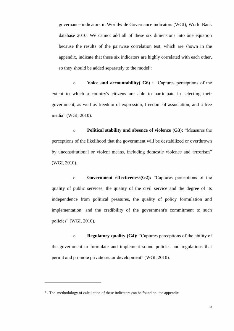
98
governance indicators in Worldwide Governance indicators (WGI), World Bank
database 2010. We cannot add all of these six dimensions into one equation
because the results of the pairwise correlation test, which are shown in the
appendix, indicate that these six indicators are highly correlated with each other,
so they should be added separately to the model4:
o Voice and accountability( G6) : “Captures perceptions of the
extent to which a country's citizens are able to participate in selecting their
government, as well as freedom of expression, freedom of association, and a free
media” (WGI, 2010).
o Political stability and absence of violence (G3): “Measures the
perceptions of the likelihood that the government will be destabilized or overthrown
by unconstitutional or violent means, including domestic violence and terrorism”
(WGI, 2010).
o Government effectiveness(G2): “Captures perceptions of the
quality of public services, the quality of the civil service and the degree of its
independence from political pressures, the quality of policy formulation and
implementation, and the credibility of the government's commitment to such
policies” (WGI, 2010).
o Regulatory quality (G4): “Captures perceptions of the ability of
the government to formulate and implement sound policies and regulations that
permit and promote private sector development” (WGI, 2010).
4 - The methodology of calculation of these indicators can be found on the appendix
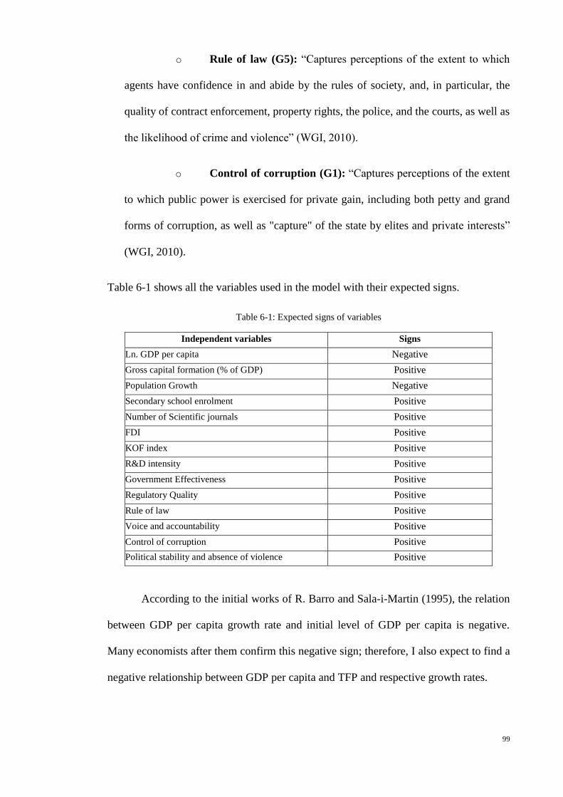
99
o Rule of law (G5): “Captures perceptions of the extent to which
agents have confidence in and abide by the rules of society, and, in particular, the
quality of contract enforcement, property rights, the police, and the courts, as well as
the likelihood of crime and violence” (WGI, 2010).
o Control of corruption (G1): “Captures perceptions of the extent
to which public power is exercised for private gain, including both petty and grand
forms of corruption, as well as "capture" of the state by elites and private interests”
(WGI, 2010).
Table 6-1 shows all the variables used in the model with their expected signs.
Table 6-1: Expected signs of variables
Independent variables Signs
Ln. GDP per capita Negative
Gross capital formation (% of GDP) Positive
Population Growth Negative
Secondary school enrolment Positive
Number of Scientific journals Positive
FDI Positive
KOF index Positive
R&D intensity Positive
Government Effectiveness Positive
Regulatory Quality Positive
Rule of law Positive
Voice and accountability Positive
Control of corruption Positive
Political stability and absence of violence Positive
According to the initial works of R. Barro and Sala-i-Martin (1995), the relation
between GDP per capita growth rate and initial level of GDP per capita is negative.
Many economists after them confirm this negative sign; therefore, I also expect to find a
negative relationship between GDP per capita and TFP and respective growth rates.

100
The relationship between the formation of capital, economic growth and
convergence is expected to be positive. Solow believed that the saving rate is constant,
however, others like Cass (1965) and Koopmans (1965) considered it as an endogenous
factor, which affects economic growth. In addition R. J. Barro (1991) discussed that
more savings shift the level of steady state upward, which increases the growth.
Moreover, several studies like those done by G. Mankiw et al. (1992), Bassanini and
Ernst (2002) and Ederveen, Groot, and Nahuis (2006) approved the positive effect of
saving rate on economic growth.
Population growth rate is a key factor to show the structure of age in an
economy and also indicates the amount of labour supply in an economy. According to
Solow (1956), the more population growth, the less capital-labour ratio an economy has,
which reduces investments in that economy. G. Mankiw et al. (1992), and S. Ederveen,
H.L.F. Groot, and R. Nahuis (2006) show that population growth has a negative effect
on growth. This research is also expecting a negative sign for population growth on
growth.
Paul M Romer (1986), in his research, discussed the role of human capital on
growth and considered it as another engine of growth. After him, several people worked
on this area and proxied different variables for measuring human capital. In general, it is
difficult to find an adequate proxy for this factor. School enrolment rate is used by G.
Mankiw et al. (1992), R. J. Barro (1991) and R. Barro and Sala-i-Martin (1995). This
study uses the secondary school enrolment variable as a proxy for human capital to
examine the effect of each on growth and to determine the effect of it on convergence
process. This is expected to have a positive sign.
The KOF index and foreign direct investment are used as proxies for
globalization. The expected sign is positive for this group of indicators. Dreher (2003)

101
introduced the KOF index, which includes three sub-indexes: economic integration,
political integration and social integration. In his paper he concludes that, in general,
globalization can promote growth. Here, in this study, we use these two indices to show
their effect on the growth and convergence process. Kottaridi (2005), Krueger and Berg
(2003), and D. Dollar and Kraay (2004) found a positive relationship between trade and
growth. We also expect to find a positive relationship. For FDI, some researchers
argued that there is a positive relationship between this and growth in countries that are
rich Blomström et al. (1997), while others believe that there is negative relationship
between them in low-income countries (Geoffrey Garrett, 2000). In this research we
investigate this relationship according to three groups of countries with different levels
of income.
According to several economists, such as Cappelen, Fagerberg, and Verspagen
(1999), and Bassanini and Ernst (2002), research intensity is an item that can increase
productivity, and, therefore, growth through improving technology. However, an
important matter here is a good combination of labour force and technology progress.
Human capital should have sufficient skills to use these technologies (Miles & Scott,
2002). Therefore, here we expect to find a positive relationship between research
intensity and growth.
Political and institutional factors are also very important in growth. As explained
in the literature review, economists use several indicators for the proxy. However, here,
for the first time, we want to examine the effect of six different variables, named as
governance indicators, which were introduced by Kaufmann et al. (2009).
102
6.2.3 Sources of Data and List of countries
6.2.3.1 Sources for Data
The sources of data used for analysis consist of:
· World Development Indicators, 2010: “World Development Indicators” (WDI) is
the primary World Bank database for development data from officially-recognized
international sources. The WDI includes data from 209 countries spanning from
1960 to 2010. It presents the most current and accurate global development data
available, and includes national, regional and global estimates.” (World Bank,
2010). This database covers 16 topics including:
1. Agriculture and rural development 2. Infrastructure
3. Aid effectiveness 4. Labour and social protection
5. Economic policy and external debt 6. Poverty
7. Education 8. Private sector
9. Energy and mining 10. Public sector
11. Environment 12. Science and technology
13. Financial sector 14. Social development
15. Health 16. Urban development
· The Worldwide Governance Indicators (WGI) project (1996-2010): the dataset
includes six dimensions of governance for 213 economies over the period 1996–
2010:
o Voice and Accountability
o Political Stability and Absence of Violence
o Government Effectiveness
o Regulatory Quality
o Rule of Law
o Control of Corruption
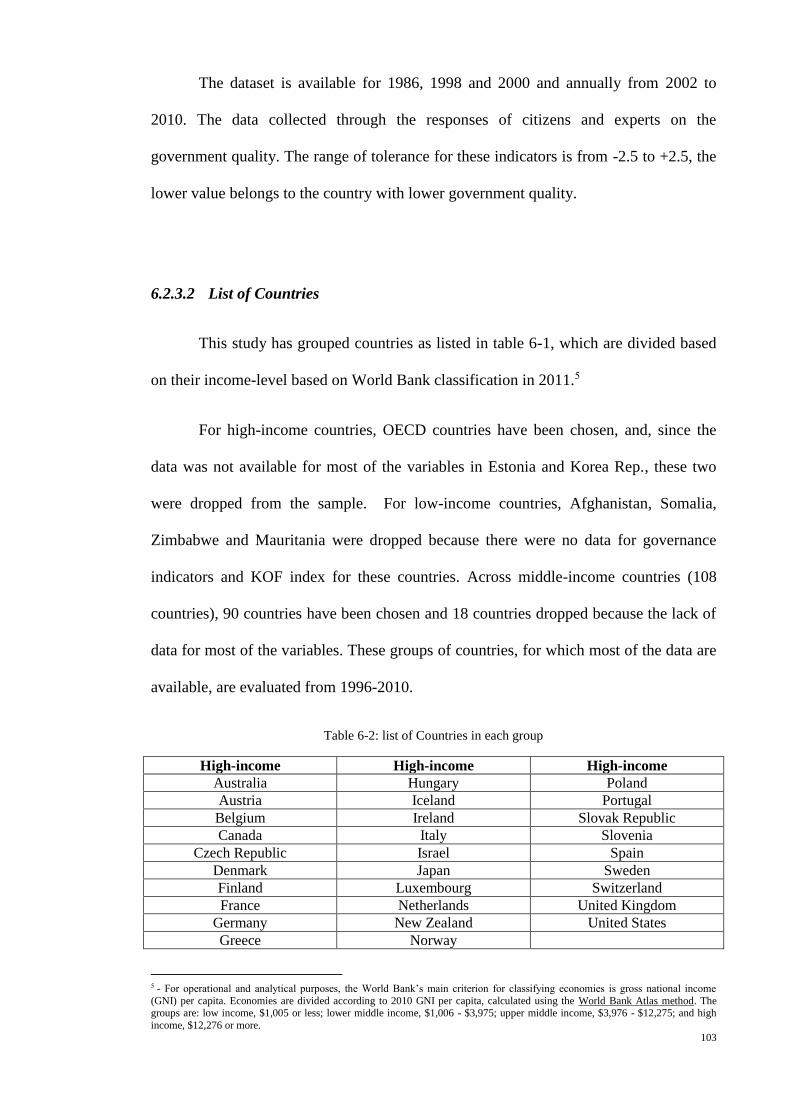
103
The dataset is available for 1986, 1998 and 2000 and annually from 2002 to
2010. The data collected through the responses of citizens and experts on the
government quality. The range of tolerance for these indicators is from -2.5 to +2.5, the
lower value belongs to the country with lower government quality.
6.2.3.2 List of Countries
This study has grouped countries as listed in table 6-1, which are divided based
on their income-level based on World Bank classification in 2011.5
For high-income countries, OECD countries have been chosen, and, since the
data was not available for most of the variables in Estonia and Korea Rep., these two
were dropped from the sample. For low-income countries, Afghanistan, Somalia,
Zimbabwe and Mauritania were dropped because there were no data for governance
indicators and KOF index for these countries. Across middle-income countries (108
countries), 90 countries have been chosen and 18 countries dropped because the lack of
data for most of the variables. These groups of countries, for which most of the data are
available, are evaluated from 1996-2010.
Table 6-2: list of Countries in each group
High-income High-income High-income
Australia Hungary Poland
Austria Iceland Portugal
Belgium Ireland Slovak Republic
Canada Italy Slovenia
Czech Republic Israel Spain
Denmark Japan Sweden
Finland Luxembourg Switzerland
France Netherlands United Kingdom
Germany New Zealand United States
Greece Norway
5 - For operational and analytical purposes, the World Bank’s main criterion for classifying economies is gross national income
(GNI) per capita. Economies are divided according to 2010 GNI per capita, calculated using the World Bank Atlas method. The groups are: low income, $1,005 or less; lower middle income, $1,006 - $3,975; upper middle income, $3,976 - $12,275; and high
income, $12,276 or more.
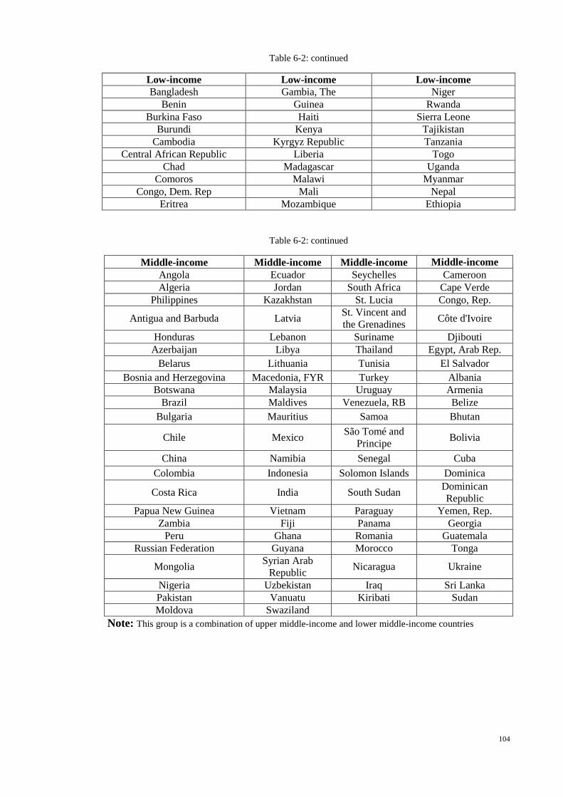
104
Table 6-2: continued
Low-income Low-income Low-income
Bangladesh Gambia, The Niger
Benin Guinea Rwanda
Burkina Faso Haiti Sierra Leone
Burundi Kenya Tajikistan
Cambodia Kyrgyz Republic Tanzania
Central African Republic Liberia Togo
Chad Madagascar Uganda
Comoros Malawi Myanmar
Congo, Dem. Rep Mali Nepal
Eritrea Mozambique Ethiopia
Table 6-2: continued
Middle-income Middle-income Middle-income Middle-income
Angola Ecuador Seychelles Cameroon
Algeria Jordan South Africa Cape Verde
Philippines Kazakhstan St. Lucia Congo, Rep.
Antigua and Barbuda Latvia St. Vincent and
the Grenadines Côte d'Ivoire
Honduras Lebanon Suriname Djibouti
Azerbaijan Libya Thailand Egypt, Arab Rep.
Belarus Lithuania Tunisia El Salvador
Bosnia and Herzegovina Macedonia, FYR Turkey Albania
Botswana Malaysia Uruguay Armenia
Brazil Maldives Venezuela, RB Belize
Bulgaria Mauritius Samoa Bhutan
Chile Mexico São Tomé and
Principe Bolivia
China Namibia Senegal Cuba
Colombia Indonesia Solomon Islands Dominica
Costa Rica India South Sudan Dominican
Republic
Papua New Guinea Vietnam Paraguay Yemen, Rep.
Zambia Fiji Panama Georgia
Peru Ghana Romania Guatemala
Russian Federation Guyana Morocco Tonga
Mongolia Syrian Arab
Republic Nicaragua Ukraine
Nigeria Uzbekistan Iraq Sri Lanka
Pakistan Vanuatu Kiribati Sudan
Moldova Swaziland
Note: This group is a combination of upper middle-income and lower middle-income countries

105
6.3 Research Hypotheses
Given the discussion of research objectives in chapter one the following
hypotheses will be tested in this research for three groups of countries with different
levels of income from the period 1996 to 2009.
Hypothesis 1: There is no difference in the explanatory power of the NCGM and
NGM across the sample of countries. There is a big disagreement between these two
schools of thought on the sources of growth: whether technological changes are the
most important sources of growth or formation of capital.
Hypothesis 2: Convergence in middle- and low-income countries is faster than in
high-income countries in both the neoclassical and new growth theories. According to
the theories of convergence, in both theories, countries that are poorer and are far away
from technology leaders tend to grow faster than rich ones or the leaders.
Hypothesis 3: Globalization, institutions and innovation factors have a positive
impact on productivity growth (as components of knowledge growth) and have the
fastest convergence speed in the sample of countries.
To show how different dimensions of technology evolved in past years, this study
follows the standard analysis of testing convergence, β convergence, for innovation
intensity, human capital, innovation, globalization and studies how their statistical
distributions have evolved over the past thirteen years and which of them have the
fastest speed among the others in each group of countries.
Hypothesis 4: Globalization can help poor countries to come out of the trap of
low-income level in both models. There are two points of view about globalization
phenomenon. One group believes that globalization is a malignant force that only helps
advanced countries to take advantage of backwardness(Carkovic & Levine, 2002;
106
Milanovic & Squire, 2005; Slaughter, 1997). However, the other group believes that
globalization can also help poor countries to come out of the low-income trap and catch
up with the rich ones(Agénor, 2004; Bhagwati & Srinivasan, 2002; Ganuza et al., 2005;
Neutel & Heshmati, 2006).
Hypothesis 5: Institutions have a positive relationship with growth in both classes
of models. Appropriate institutions and government policies can help countries further
from their leader to take advantage of this backwardness and grow faster.
107
7 Chapter 7
Estimation Results
7.1 Introduction
In presenting the empirical results, this chapter seeks to do the following. The
overall objective is to provide an empirical basis for the many theories of convergence
and to benchmark other research on these theories. The first specific objective is to test
the convergence hypothesis across different countries using the neoclassical and new
growth models. The second is to evaluate the applicability of these models to the data
set we are using. The third is to study the explanatory power of additional variables like
globalization, innovation and institutions on growth that have not been taken into
account in existing studies. In doing so, we shall also explore whether the level of
economic development matters in the explanatory power of these variables.
The rest of this chapter is as follows. The next section reports the results of β
convergence in terms of GDP per capita based on augmented Solow-Swan regression
(neoclassical growth regression) in low-income, middle-income and high-income
countries. It also examines the role played by the variables cited above in explaining β
convergence. The results of sigma convergence are also reported in this section. Section
three is about the results of β convergence in terms of GDP per capita based on applying
new growth regression in low-income, middle-income and high-income countries. This
section also reports the results of φ convergence in terms of each technology dimension
that is considered in this study – innovation, globalization and institutions – to show
how the technology gap evolved in recent years. Finally, section four is the conclusion.
108
7.2 Neoclassical growth model
This section tests the β convergence hypothesis in terms of GDP per capita in
three groups of countries – high-income, middle-income and low-income countries –
using the DSGMM6 method. As said before, convergence happens when there is a
negative relationship between the average annual growth rate of GDP per capita and
initial amount of GDP per capita, which means that countries that are far from their
steady state (poor countries) can grow faster and reach to the steady state growth path
rather than those that are closer (rich countries). Therefore, if the sign of initial GDP
per capita is negative it means that convergence happened across countries.
β convergence is tested by applying equations (7-1) and (7-2) in samples of low-
income, middle-income and high-income countries between 1996 and 2010 in terms of
GDP per capita based on the neoclassical theory.
∆𝐿𝑛(𝑦𝑖,𝑡) = 𝜃2𝑙𝑛𝑠ℎ,𝑖,𝑡 + 𝜃3𝑙𝑛𝑠𝑘𝑖,𝑡 − 𝜃4ln (𝑛𝑖,𝑡 + 𝑔 + 𝛿) + 𝜃5𝐿𝑛(𝑦𝑖,𝑡−1) + 휁𝑡 + 𝜌𝑖 + 휀𝑖,𝑡
(7-1)
∆𝐿𝑛(𝑦𝑖,𝑡) = 𝜃2𝑙𝑛𝑠ℎ,𝑖,𝑡 + 𝜃3𝑙𝑛𝑠𝑘𝑖,𝑡 + 𝜃4 ln(1 + 𝐺𝐿𝑂𝐵𝑖,𝑡) + 𝜃5 ln(1 + 𝐼𝑁𝑂𝑖,𝑡) +
𝜃6 ln(1 + 𝐼𝑁𝑆𝑖,𝑡) − 𝜃7ln (𝑛𝑖,𝑡 + 𝑔 + 𝛿) + 𝜃8𝐿𝑛(𝑦𝑖,𝑡−1) + 휁𝑡 + 𝜌𝑖 + 휀𝑖,𝑡 (7-2)
All the variables are taken in natural log form. In addition, for institutions,
innovation and globalization in equation (7-2) all the variables are normalized before
entering for estimation to become between zero and one. Therefore in this form they can
act like an accelerator coefficient for the human capital factor.
6 - Dynamic system Generalized method of moments

109
7.2.1 Testing β Convergence in First Augmented Solow-Swan Model
We begin with the augmented Solow-Swan model (equation 7-1). Table (7-1)
reports the results for the whole as well as the split samples.
Table 7-1 Testing convergence in the first Augmented Solow-Swan Model using dynamic system GMM
VARIABLES Whole sample High-income Low-income Middle-income
∆𝐿𝑛(𝑦𝑖,𝑡−1) 0.139*** 0.196*** -0.118** 0.0164*
(0.00483) (0.0278) (0.0479) (0.00994)
𝐿𝑛(𝑦𝑖,𝑡−1) -0.00106*** -0.0139*** -0.0212 -0.478***
(3.26e-05) (0.369) (0.415) (0.0370)
𝑙𝑛𝑠ℎ,𝑖,𝑡 0.158*** 0.280 0.191** 1.198***
(0.00448) (0.388) (0.841) (0.0830)
𝑙𝑛𝑠𝑘𝑖,𝑡 2.157*** 3.484*** 0.231*** 4. 609*
(1.00496) (1.067) (0.0806) (1.0313)
ln (𝑛𝑖,𝑡 + 0.05) -1.208*** -0.115*** -0.218*** -0.022***
(0.0817) (0.0803) (0.00989) (0.00789)
Implied λ 0.0000707 0.00107 … 0.0500
Observations 1,616 392 298 1231
Number of code 149 29 30 90
Sargan test,P-value 0.3435 1.0000 0.9987 1.0000
AR(1),P-value 0.0000 0.0042 0.3226 0.0003
AR(2),P-value 0.0768 0.2548 0.3654 0.9269 Note: Standard errors in parentheses,*** p<0.01, ** p<0.05, * p<0.1, time dummies are also included in
estimated regression, the results are not reported here.
According to the Augmented Solow-Swan regression we are expecting a
positive sign for θ2 and θ3 and negative for θ4. As can be seen from table (7-1), we can
see that for all of the variables this prediction is true for all groups. However, the
significance and magnitude coefficient of each variable are different in different groups,
which will be discussed later.
The other implication of this model is about speed of convergence, which is calculated
by the following formula (G. Mankiw et al., 1992):
Implies speed of convergence: θ = (𝑒−𝜆𝑡 − 1) → 𝜆 = −1/𝑡[𝐿𝑛(1 + 𝜃)]

110
The implied speed of convergence is reported in the same table (7-1). As can be
seen, the speed of convergence is 0.0000707 for the whole sample, 0.05001 for middle-
income countries, 0.001 for high-income countries and no convergence for low-income
countries. This means that middle-income countries of the sample move halfway to the
steady state in about 13 years,7 for high-income countries the speed of countries is very
slow and takes decades to move to the steady state. In addition, the results show no
convergence according to this model for low-income countries. The results for middle-
income countries is much larger from the results of G. Mankiw et al. (1992), which
reported a speed of convergence for 0.0137 a year using the same regression, and lower
than that found by Malcolm Knight, Norman Loayza, and Delano Villanueva (1993),
which is 0.0631 for developing countries, also using the same regression. These huge
differences can be discussed by the method and nature of the data that they used for
estimating the growth regressions. In their study, G. Mankiw et al. (1992) did not care
about the country specific effect and the relationship that it could have with other
explanatory variables. It is true that Knight applied panel data analysis but even in his
study he ignored the problem of endogeneity of some variables in the model and also
the fact that the lagged level of the dependent variable, in this study, lagged GDP
growth, can also affect the dependent variable. Therefore, they ignored the problem of
endogeneity, which, in this study, by applying dynamic system GMM, we account for
country specific effects by taking first difference from the regression and we account for
omitted and endogeneity by adding instrument variables to the model. Therefore the
coefficients are no longer biased towards zero.
7 The formula for calculation half-life is T= Ln (2)/ λ, T is number of years.
111
7.2.1.1 Determinants of Growth in the First Augmented Solow-Swan Model
Table (7-1) also reports the effects of investing in human capital, physical
capital and population growth on economic growth across these groups of countries. As
can be seen the signs of investing in physical capital are positive and significant in all
groups. However, it is less productive for low-income countries compared to high-
income and middle-income countries. Moreover, between high-income and middle-
income countries, it is stronger in middle-income countries.
For investing in education for the secondary level, as the results show, it is less
productive for low-income countries than middle-income countries. This means that by
investing more in their secondary education middle-income countries can speed their
economic growth. The sign of this variable is positive but not significant for high-
income countries, meaning that they already have enough level of human capital with
secondary education and investing in this section will not affect growth. This is
consistent with the argument of M. R. Islam (2010) who said that “advanced countries
are more likely to engage in innovating new technologies which required highly skilled
human capital”.
The growth rate of population has a negative and significant effect on GDP
growth, especially when we eliminate middle-income and high-income countries from
the sample.
112
7.2.2 Testing β Convergence in the Second Augmented Solow-Swan Model
Table (7-2), (7-3), (7-4) and (7-5) report the second augmented version of
Solow-Swan model, equation (7-2), by including institutions, globalization and
innovation variables to the model in the whole sample as well as the split ones. By
including globalization indicators, institutions factors and innovation proxies we try to
control the unobserved effects. The important fact here is the way that we apply these
variables into the model. According to the neoclassical growth theory the accumulation
of capital is important in explaining the growth rate across countries so we apply these
variables through the accumulation of human capital rather than endogenizing them
through technology to the model. This means that these factors are more closely related
as factors that can speed up the process of capital accumulation for increasing
production than to the efficiency variable.
First, we discuss the speed of convergence in each group of countries. As can be
seen, each of the governance indicators is included separately; therefore, we have six
equations.
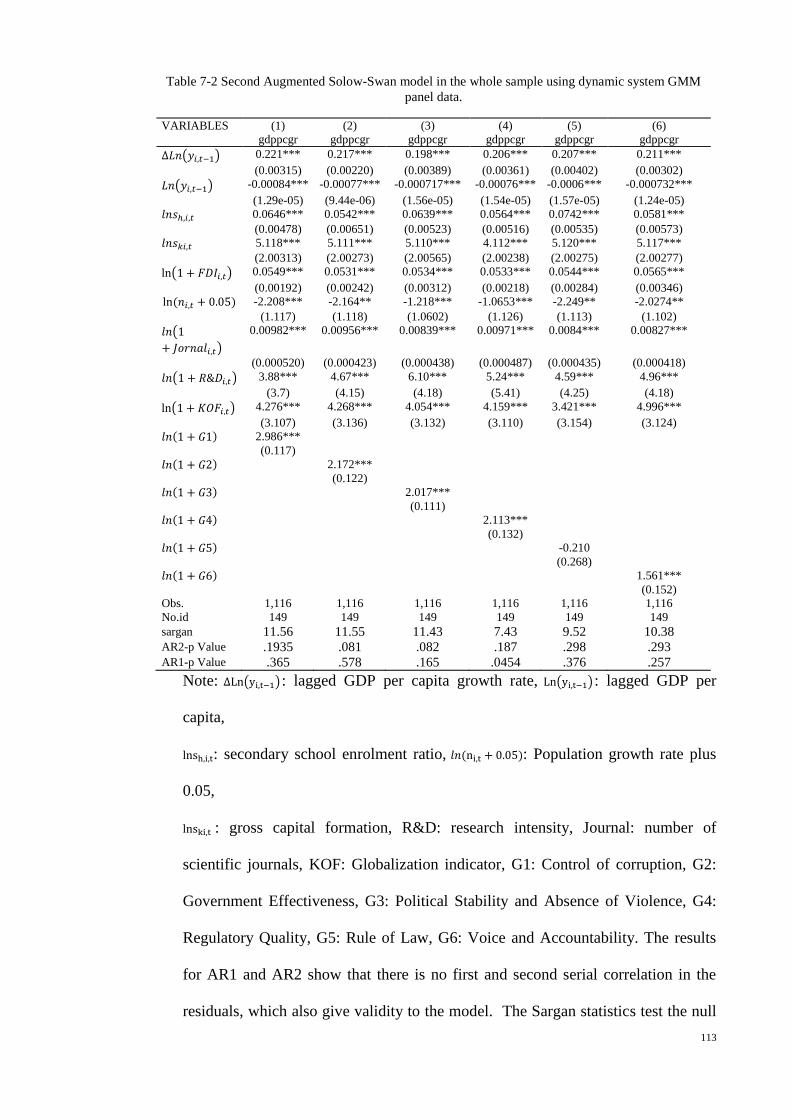
113
Table 7-2 Second Augmented Solow-Swan model in the whole sample using dynamic system GMM
panel data.
VARIABLES (1) (2) (3) (4) (5) (6)
gdppcgr gdppcgr gdppcgr gdppcgr gdppcgr gdppcgr
∆𝐿𝑛(𝑦𝑖,𝑡−1) 0.221*** 0.217*** 0.198*** 0.206*** 0.207*** 0.211***
(0.00315) (0.00220) (0.00389) (0.00361) (0.00402) (0.00302)
𝐿𝑛(𝑦𝑖,𝑡−1) -0.00084*** -0.00077*** -0.000717*** -0.00076*** -0.0006*** -0.000732***
(1.29e-05) (9.44e-06) (1.56e-05) (1.54e-05) (1.57e-05) (1.24e-05)
𝑙𝑛𝑠ℎ,𝑖,𝑡 0.0646*** 0.0542*** 0.0639*** 0.0564*** 0.0742*** 0.0581***
(0.00478) (0.00651) (0.00523) (0.00516) (0.00535) (0.00573)
𝑙𝑛𝑠𝑘𝑖,𝑡 5.118*** 5.111*** 5.110*** 4.112*** 5.120*** 5.117***
(2.00313) (2.00273) (2.00565) (2.00238) (2.00275) (2.00277)
ln(1 + 𝐹𝐷𝐼𝑖,𝑡) 0.0549*** 0.0531*** 0.0534*** 0.0533*** 0.0544*** 0.0565***
(0.00192) (0.00242) (0.00312) (0.00218) (0.00284) (0.00346)
ln (𝑛𝑖,𝑡 + 0.05) -2.208*** -2.164** -1.218*** -1.0653*** -2.249** -2.0274**
(1.117) (1.118) (1.0602) (1.126) (1.113) (1.102)
𝑙𝑛(1
+ 𝐽𝑜𝑟𝑛𝑎𝑙𝑖,𝑡)
0.00982*** 0.00956*** 0.00839*** 0.00971*** 0.0084*** 0.00827***
(0.000520) (0.000423) (0.000438) (0.000487) (0.000435) (0.000418)
𝑙𝑛(1 + 𝑅&𝐷𝑖,𝑡) 3.88*** 4.67*** 6.10*** 5.24*** 4.59*** 4.96***
(3.7) (4.15) (4.18) (5.41) (4.25) (4.18)
ln(1 + 𝐾𝑂𝐹𝑖,𝑡) 4.276*** 4.268*** 4.054*** 4.159*** 3.421*** 4.996***
(3.107) (3.136) (3.132) (3.110) (3.154) (3.124)
𝑙𝑛(1 + 𝐺1) 2.986***
(0.117)
𝑙𝑛(1 + 𝐺2) 2.172***
(0.122)
𝑙𝑛(1 + 𝐺3) 2.017***
(0.111)
𝑙𝑛(1 + 𝐺4) 2.113***
(0.132)
𝑙𝑛(1 + 𝐺5) -0.210
(0.268)
𝑙𝑛(1 + 𝐺6) 1.561***
(0.152)
Obs. 1,116 1,116 1,116 1,116 1,116 1,116
No.id 149 149 149 149 149 149
sargan 11.56 11.55 11.43 7.43 9.52 10.38
AR2-p Value .1935 .081 .082 .187 .298 .293
AR1-p Value .365 .578 .165 .0454 .376 .257
Note: ∆Ln(yi,t−1): lagged GDP per capita growth rate, Ln(yi,t−1): lagged GDP per
capita,
lnsh,i,t: secondary school enrolment ratio, 𝑙𝑛 (ni,t + 0.05): Population growth rate plus
0.05,
lnski,t : gross capital formation, R&D: research intensity, Journal: number of
scientific journals, KOF: Globalization indicator, G1: Control of corruption, G2:
Government Effectiveness, G3: Political Stability and Absence of Violence, G4:
Regulatory Quality, G5: Rule of Law, G6: Voice and Accountability. The results
for AR1 and AR2 show that there is no first and second serial correlation in the
residuals, which also give validity to the model. The Sargan statistics test the null

114
hypothesis of the correct model specification and validity of the instruments. As
the results show we cannot reject the null hypothesis, which shows that the
instruments are valid. Time dummies are also included, which is not reported here.

115
Table 7-3 Second Augmented Solow-Swan model in high-income countries using dynamic system GMM
panel data
VARIABLES Eq.(1) (2) (3) (4) (5) (6)
∆𝐿𝑛(𝑦𝑖,𝑡−1) 0.753*** 0.688*** 0.708*** 0.714*** 0.723*** 0.702***
(0.0322) (0.0604) (0.0617) (0.0518) (0.0648) (0.0646)
𝐿𝑛(𝑦𝑖,𝑡−1) -0.4108*** -0.41*** -0.4117*** -0.4104*** -0.4107*** -0.4106***
(7.42e-05) (7.24e-05) (5.74e-05) (7.06e-05) (6.53e-05) (6.34e-05)
𝑙𝑛𝑠ℎ,𝑖,𝑡 -0.0481*** -0.0392*** -0.0430*** -0.0176 -0.0356*** -0.0279**
(0.00447) (0.00737) (0.00784) (0.0168) (0.00757) (0.0128)
𝑙𝑛𝑠𝑘𝑖,𝑡 4.070*** 4.184*** 4.896*** 4.969*** 4.503*** 3.958**
(1.557) (1.523) (1.563) (1.519) (1.555) (1.543)
ln(1 + 𝐹𝐷𝐼𝑖,𝑡) 0.970*** 1.071*** 1.055*** 1.136*** 1.045*** 0.880***
(0.150) (0.196) (0.169) (0.162) (0.177) (0.162)
ln (𝑛𝑖,𝑡 + 0.05) -0.346*** -0.246** 1.366*** 0.157** -0.326*** 1.750**
(0.887) (0.791) (1.250) (0.752) (0.907) (0.812)
𝑙𝑛(1 + 𝐽𝑜𝑟𝑛𝑎𝑙𝑖,𝑡) 0.538** 0.449*** 0.544** 0.455** 0.540** 0.563***
(0.153) (0.154) (0.159) (0.154) (0.154) (0.152)
𝑙𝑛(1 + 𝑅&𝐷𝑖,𝑡) 5.50** 4.34** 9.78*** 6.17*** 6.05*** 6.62***
(2.78) (2.06) (2.30) (2.35) (2.06) (2.01)
ln(1 + 𝐾𝑂𝐹𝑖,𝑡) 3.085*** 3.081*** 3.299*** 2.870** 2.912*** 1.584**
(2.331) (2.600) (2.714) (1.149) (2.434) (2.781)
𝑙𝑛(1 + 𝐺1) 2.563**
(1.291)
𝑙𝑛(1 + 𝐺2) 3.689***
(2.803)
𝑙𝑛(1 + 𝐺3) 3.390***
(1.141)
𝑙𝑛(1 + 𝐺4) 6.015***
(3.931)
𝑙𝑛(1 + 𝐺5) 3.857**
(1.507)
𝑙𝑛(1 + 𝐺6) 1.626
(1.765)
Obs. 388 388 388 388 388 388
No.id 29 29 29 29 29 29
sargan 13.68 13.25 12.63 8.403 12.72 11.28
AR2-p Value .0935 .181 .092 .287 .198 .193
AR1-p Value .395 .538 .1621 .0484 .362 .245
Note: ∆Ln(yi,t−1): lagged GDP per capita growth rate, Ln(yi,t−1): lagged GDP per
capita,
lnsh,i,t: secondary school enrolment ratio, 𝑙𝑛 (ni,t + 0.05): Population growth rate plus
0.05,
lnski,t : gross capital formation, R&D: research intensity, Journal: number of
scientific journals, KOF: Globalization indicator, G1: Control of corruption, G2:
Government Effectiveness, G3: Political Stability and Absence of Violence, G4:
Regulatory Quality, G5: Rule of Law, G6: Voice and Accountability. The results

116
for AR1 and AR2 show that there is no first and second serial correlation in the
residuals which also give validity to the model. The Sargan statistics tests the null
hypothesis of correct model specification and validity of instruments. As the results
show we cannot reject the null hypothesis, which shows that the instruments are
valid. Time dummies are also included, which is not reported here.
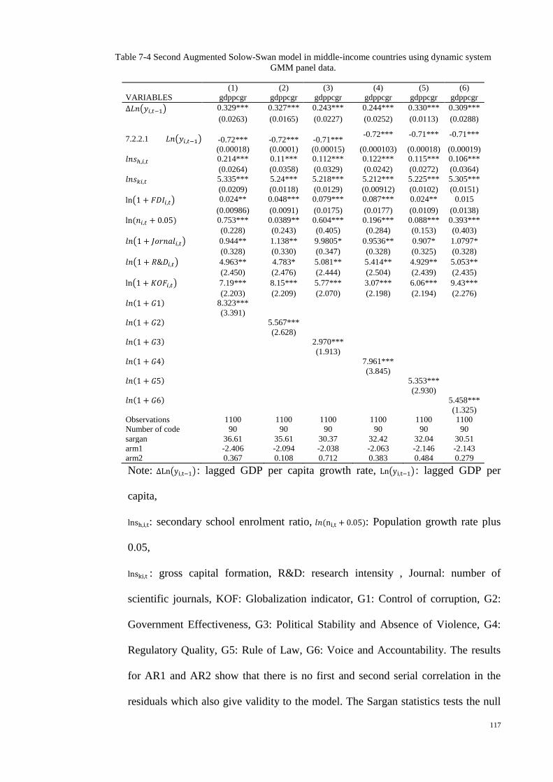
117
Table 7-4 Second Augmented Solow-Swan model in middle-income countries using dynamic system
GMM panel data.
(1) (2) (3) (4) (5) (6)
VARIABLES gdppcgr gdppcgr gdppcgr gdppcgr gdppcgr gdppcgr
∆𝐿𝑛(𝑦𝑖,𝑡−1) 0.329*** 0.327*** 0.243*** 0.244*** 0.330*** 0.309***
(0.0263) (0.0165) (0.0227) (0.0252) (0.0113) (0.0288)
7.2.2.1 𝐿𝑛(𝑦𝑖,𝑡−1) -0.72*** -0.72*** -0.71*** -0.72*** -0.71*** -0.71***
(0.00018) (0.0001) (0.00015) (0.000103) (0.00018) (0.00019)
𝑙𝑛𝑠ℎ,𝑖,𝑡 0.214*** 0.11*** 0.112*** 0.122*** 0.115*** 0.106***
(0.0264) (0.0358) (0.0329) (0.0242) (0.0272) (0.0364)
𝑙𝑛𝑠𝑘𝑖,𝑡 5.335*** 5.24*** 5.218*** 5.212*** 5.225*** 5.305***
(0.0209) (0.0118) (0.0129) (0.00912) (0.0102) (0.0151)
ln(1 + 𝐹𝐷𝐼𝑖,𝑡) 0.024** 0.048*** 0.079*** 0.087*** 0.024** 0.015
(0.00986) (0.0091) (0.0175) (0.0177) (0.0109) (0.0138)
ln (𝑛𝑖,𝑡 + 0.05) 0.753*** 0.0389** 0.604*** 0.196*** 0.088*** 0.393***
(0.228) (0.243) (0.405) (0.284) (0.153) (0.403)
𝑙𝑛(1 + 𝐽𝑜𝑟𝑛𝑎𝑙𝑖,𝑡) 0.944** 1.138** 9.9805* 0.9536** 0.907* 1.0797*
(0.328) (0.330) (0.347) (0.328) (0.325) (0.328)
𝑙𝑛(1 + 𝑅&𝐷𝑖,𝑡) 4.963** 4.783* 5.081** 5.414** 4.929** 5.053**
(2.450) (2.476) (2.444) (2.504) (2.439) (2.435)
ln(1 + 𝐾𝑂𝐹𝑖,𝑡) 7.19*** 8.15*** 5.77*** 3.07*** 6.06*** 9.43***
(2.203) (2.209) (2.070) (2.198) (2.194) (2.276)
𝑙𝑛(1 + 𝐺1) 8.323***
(3.391)
𝑙𝑛(1 + 𝐺2) 5.567***
(2.628)
𝑙𝑛(1 + 𝐺3) 2.970***
(1.913)
𝑙𝑛(1 + 𝐺4) 7.961***
(3.845)
𝑙𝑛(1 + 𝐺5) 5.353***
(2.930)
𝑙𝑛(1 + 𝐺6) 5.458***
(1.325)
Observations 1100 1100 1100 1100 1100 1100
Number of code 90 90 90 90 90 90
sargan 36.61 35.61 30.37 32.42 32.04 30.51
arm1 -2.406 -2.094 -2.038 -2.063 -2.146 -2.143
arm2 0.367 0.108 0.712 0.383 0.484 0.279
Note: ∆Ln(yi,t−1): lagged GDP per capita growth rate, Ln(yi,t−1): lagged GDP per
capita,
lnsh,i,t: secondary school enrolment ratio, 𝑙𝑛 (ni,t + 0.05): Population growth rate plus
0.05,
lnski,t : gross capital formation, R&D: research intensity , Journal: number of
scientific journals, KOF: Globalization indicator, G1: Control of corruption, G2:
Government Effectiveness, G3: Political Stability and Absence of Violence, G4:
Regulatory Quality, G5: Rule of Law, G6: Voice and Accountability. The results
for AR1 and AR2 show that there is no first and second serial correlation in the
residuals which also give validity to the model. The Sargan statistics tests the null

118
hypothesis of correct model specification and validity of instruments. As the results
show we cannot reject the null hypothesis, which shows that the instruments are
valid. Time dummies are also included, which is not reported here.
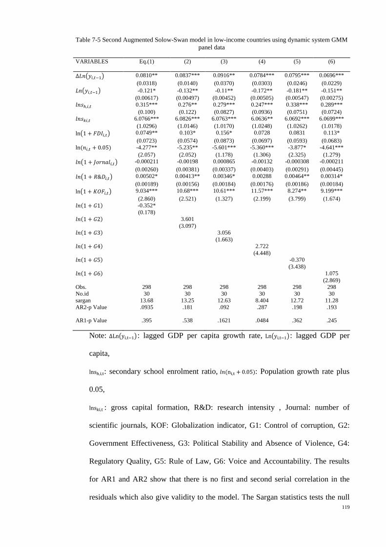
119
Table 7-5 Second Augmented Solow-Swan model in low-income countries using dynamic system GMM
panel data
VARIABLES Eq.(1) (2) (3) (4) (5) (6)
∆𝐿𝑛(𝑦𝑖,𝑡−1) 0.0810** 0.0837*** 0.0916** 0.0784*** 0.0795*** 0.0696***
(0.0318) (0.0140) (0.0370) (0.0303) (0.0246) (0.0229)
𝐿𝑛(𝑦𝑖,𝑡−1) -0.121* -0.132** -0.11** -0.172** -0.181** -0.151**
(0.00617) (0.00497) (0.00452) (0.00505) (0.00547) (0.00275)
𝑙𝑛𝑠ℎ,𝑖,𝑡 0.315*** 0.276** 0.279*** 0.247*** 0.338*** 0.289***
(0.100) (0.122) (0.0827) (0.0936) (0.0751) (0.0724)
𝑙𝑛𝑠𝑘𝑖,𝑡 6.0766*** 6.0826*** 6.0763*** 6.0636** 6.0692*** 6.0699***
(1.0296) (1.0146) (1.0170) (1.0248) (1.0262) (1.0178)
ln(1 + 𝐹𝐷𝐼𝑖,𝑡) 0.0749** 0.103* 0.156* 0.0728 0.0831 0.113*
(0.0723) (0.0574) (0.0873) (0.0697) (0.0593) (0.0683)
ln (𝑛𝑖,𝑡 + 0.05) -4.277** -5.235** -5.601*** -5.360*** -3.877* -4.641***
(2.057) (2.052) (1.178) (1.306) (2.325) (1.279)
𝑙𝑛(1 + 𝐽𝑜𝑟𝑛𝑎𝑙𝑖,𝑡) -0.000211 -0.00198 0.000865 -0.00132 -0.000308 -0.000211
(0.00260) (0.00381) (0.00337) (0.00403) (0.00291) (0.00445)
𝑙𝑛(1 + 𝑅&𝐷𝑖,𝑡) 0.00502* 0.00413** 0.00346* 0.00288 0.00464** 0.00314*
(0.00189) (0.00156) (0.00184) (0.00176) (0.00186) (0.00184)
ln(1 + 𝐾𝑂𝐹𝑖,𝑡) 9.034*** 10.68*** 10.61*** 11.57*** 8.274** 9.199***
(2.860) (2.521) (1.327) (2.199) (3.799) (1.674)
𝑙𝑛(1 + 𝐺1) -0.352*
(0.178)
𝑙𝑛(1 + 𝐺2) 3.601
(3.097)
𝑙𝑛(1 + 𝐺3) 3.056
(1.663)
𝑙𝑛(1 + 𝐺4) 2.722
(4.448)
𝑙𝑛(1 + 𝐺5) -0.370
(3.438)
𝑙𝑛(1 + 𝐺6) 1.075
(2.869)
Obs. 298 298 298 298 298 298
No.id 30 30 30 30 30 30
sargan 13.68 13.25 12.63 8.404 12.72 11.28
AR2-p Value .0935 .181 .092 .287 .198 .193
AR1-p Value .395 .538 .1621 .0484 .362 .245
Note: ∆Ln(yi,t−1): lagged GDP per capita growth rate, Ln(yi,t−1): lagged GDP per
capita,
lnsh,i,t: secondary school enrolment ratio, 𝑙𝑛 (ni,t + 0.05): Population growth rate plus
0.05,
lnski,t : gross capital formation, R&D: research intensity , Journal: number of
scientific journals, KOF: Globalization indicator, G1: Control of corruption, G2:
Government Effectiveness, G3: Political Stability and Absence of Violence, G4:
Regulatory Quality, G5: Rule of Law, G6: Voice and Accountability. The results
for AR1 and AR2 show that there is no first and second serial correlation in the
residuals which also give validity to the model. The Sargan statistics tests the null

120
hypothesis of correct model specification and validity of instruments. As the results
show we cannot reject the null hypothesis, which shows that the instruments are
valid. Time dummies are also included, which is not reported here.
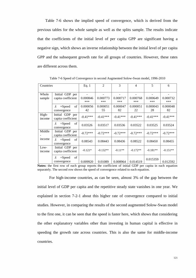
121
Table 7-6 shows the implied speed of convergence, which is derived from the
previous tables for the whole sample as well as the splits sample. The results indicate
that the coefficients of the initial level of per capita GPP are significant having a
negative sign, which shows an inverse relationship between the initial level of per capita
GPP and the subsequent growth rate for all groups of countries. However, these rates
are different across them.
Table 7-6 Speed of Convergence in second Augmented Solow-Swan model, 1996-2010
Countries Eq. 1 2 3 4 5 6
Whole
sample
Initial GDP per
capita coefficient
-
0.000846
***
-
0.000773
***
-
0.000717
***
-
0.000768
***
-
0.000649
***
-
0.000732
***
𝜆 =Speed of
convergence
0.000056
42
0.000051
55
0.000047
82
0.000051
22
0.000043
28
0.000048
82
High-
income
Initial GDP per
capita coefficient -0.41*** -0.41*** -0.41*** -0.41*** -0.41*** -0.41***
𝜆 =Speed of
convergence 0.03526 0.03517 0.03536 0.03522 0.03525 0.03524
Middle
-
income
Initial GDP per
capita coefficient -0.72*** -0.72*** -0.72*** -0.72*** -0.72*** -0.72***
𝜆 =Speed of
convergence 0.08543 0.08443 0.08436 0.08522 0.08450 0.08455
Low-
income
Initial GDP per
capita coefficient -0.121* -0.132** -0.11** -0.172** -0.181** -0.151**
𝜆 =Speed of
convergence 0.009920 0.01089 0.008964 0.014519 0.015359
0.012592
Notes: the first row of each group reports the coefficient of initial GDP per capita in each equation
separately. The second row shows the speed of convergence related to each equation.
For high-income countries, as can be seen, almost 3% of the gap between the
initial level of GDP per capita and the repetitive steady state vanishes in one year. We
explained in section 7-2-1 about this higher rate of convergence compared to initial
studies. However, in comparing the results of the second augmented Solow-Swan model
to the first one, it can be seen that the speed is faster here, which shows that considering
the other explanatory variables other than investing in human capital is effective in
speeding the growth rate across countries. This is also the same for middle-income
countries.

122
For middle-income countries, on average, almost 8% of the gap between the
initial level of GDP per capita and the repetitive steady state vanishes in one year. This
result supports the idea of convergence, which means that countries far away from the
steady state growth path can grow faster.
Finally, for low-income countries 1% of the gap between the initial level of GDP
per capita and the repetitive steady state vanishes in one year. As can be seen, in the
first augmented Solow-Swan model there was no convergence across low-income
countries, however, convergence appears after adding these explanatory variables to the
model. This means that by considering these variables for controlling the steady state,
convergence could emerge even in low-income countries albeit at a slower rate, which
raises the idea of income threshold. Countries should reach to a certain level of income
to be capable of taking advantage of the advanced technologies that is transferring from
the frontier. The results of the explanatory variables in low-income countries also
support this idea.
To sum up, in comparing the results in these three groups, it shows that the
convergence rate is much higher for middle-income countries than for high-income
countries. This is consistent with the convergence hypothesis, which said that countries
far away from their steady state could grow faster than rich ones. However, the results
of the low-income group contradict the hypothesis. Indeed, these results suggest that
convergence is not monotonic with respect to income. An income threshold may need
to be reached before convergence occurs. Countries below that threshold are caught in
a poverty trap from which it takes a long time to escape.8
8 Sachs, (2000) made a similar argument about low income / low institutional capacity countries never being able to take advantage
of technologies like the Internet.

123
7.2.2.2 Determinants of Growth in second Augmented Solow-Swan Model
Tables (7-7),(7-8), (7-9) ,(7-10) and (7-11) report the effects of investing in
human capital, physical capital, population growth, globalization indicators, FDI and
KOF index, institutions factor, R&D inensity and number of scientific journals on
economic growth across these groups of countries.
The estimated coefficient for investing in education is positive and significant
for the whole sample, while by eliminating middle-income and low-income countries
from the sample the coefficient becomes negative and significant. This result contradicts
what R. J. Barro (1991), G. Mankiw et al. (1992) and others, who use cross sectional
data analyses, found in their studies. One explanation for this result is that when the
time dimension is added to the education variable it means that in addition to cross
country difference we also consider changes in human capital over time in each country.
Why are the coefficients negative in high-income countries but remaining positive for
middle-income and low-income countries? This indicates that while investing in the
secondary level of education increased in high-income countries between 1996 and
2010, output growth fell. However, this story is not true for middle-income and
especially for low-income countries, where a one point increase in investing in
education will increase their GDP growth by 0.3 percentage points. The explanation for
this might be because for middle-income and low-income countries the cross sectional
effects are strong enough to overcome the time series relations.
Table 7-7 The results for secondary school enrolment ratio in both models
Model Variable
Whole
sample
High-
income
Low-
income
Middle-
income
First Model 𝑙𝑛𝑠ℎ,𝑖,𝑡 0.158*** 0.280 0.191** 1.198***
Second Model 𝑙𝑛𝑠ℎ,𝑖,𝑡 0.0646*** -0.048*** 0.315*** 0.214*** Note: This table is derived from previous tables. For the second model, since the results of all 6 equations
were familiar, we just put the results of the first equation.

124
Furthermore, as the results show, the coefficients are stronger for low-income
than for middle-income countries. This means that low-income countries, by investing
more in their secondary education level, can speed their economic growth. This result is
not consistent with the first model, where investing in education at the secondary level
was less productive for low-income countries than middle-income countries. Our
explanation for this result is that it seems that the quality of education investment
increases when the technology can transfer across low-income countries through
globalization.
The sign for investing in physical capital is positive and significant in the whole
sample and it is the strongest amongst the other variables. A one point increase in the
formation of physical capital increases the GDP growth rate by 6 percentage points.
When the middle-income and low-income countries are eliminated from the sample, the
sign is still positive and a one point increases in the formation of physical capital
increases the GDP growth rate by 4 percentage points. For middle-income countries
and low-income countries it is the same and the sign is positive and significant and a 5
percentage and 6 percentage point variation in GDP growth can be explained by the
physical capital accumulation in these two groups of countries, respectively.
Table 7-8 The results for investment in physical capital in both models
Model Variable
Whole
sample
High-
income
Low-
income
Middle-
income
First Model 𝑙𝑛𝑠𝑘𝑖,𝑡 2.157*** 3.484*** 0.231*** 4. 609*
Second Model 𝑙𝑛𝑠𝑘𝑖,𝑡 6.118*** 4.070*** 6.076*** 5.335*** Note: This table is derived from previous tables. For the second model, since the results of all 6 equations
were familiar, we just put the results of the first equation in this table.
As can be seen, the coefficients for investment in physical capital are larger in
all groups when proxies like FDI, KOF index, institutions, R&D intensity are added to
the model. Furthermore, the coefficient of investment in physical capital is largest in
low-income countries compared to the middle-income and high-income countries, and,
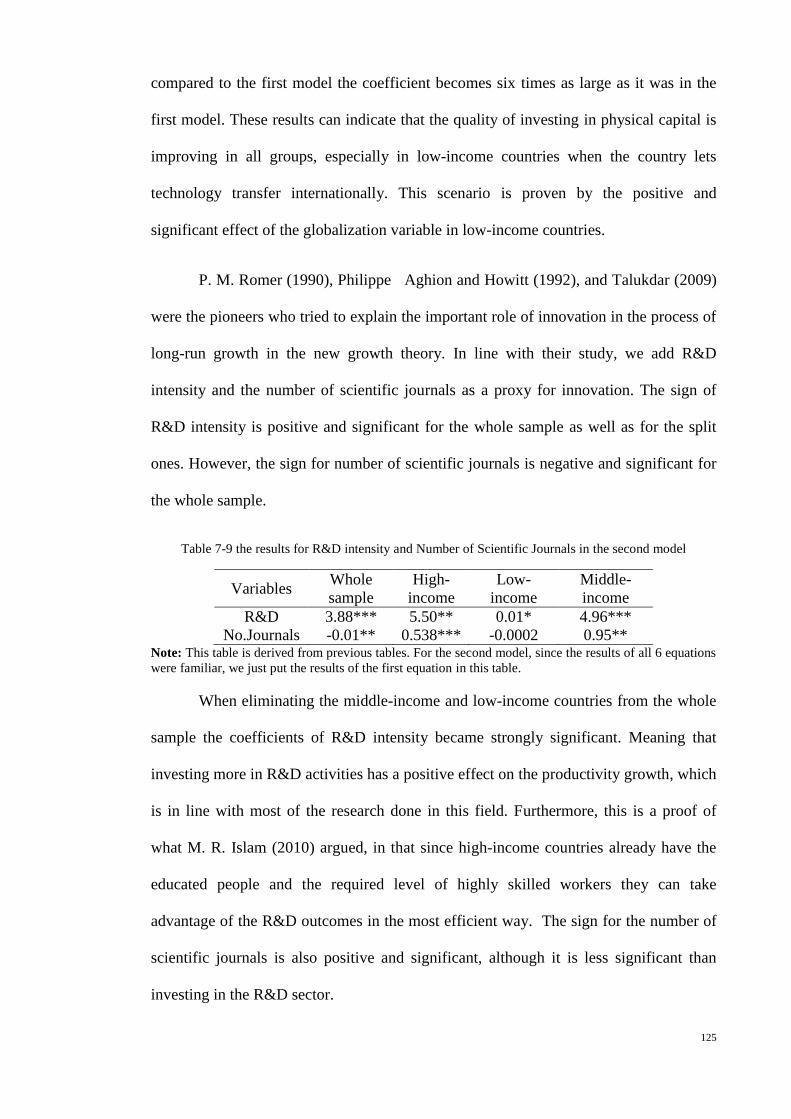
125
compared to the first model the coefficient becomes six times as large as it was in the
first model. These results can indicate that the quality of investing in physical capital is
improving in all groups, especially in low-income countries when the country lets
technology transfer internationally. This scenario is proven by the positive and
significant effect of the globalization variable in low-income countries.
P. M. Romer (1990), Philippe Aghion and Howitt (1992), and Talukdar (2009)
were the pioneers who tried to explain the important role of innovation in the process of
long-run growth in the new growth theory. In line with their study, we add R&D
intensity and the number of scientific journals as a proxy for innovation. The sign of
R&D intensity is positive and significant for the whole sample as well as for the split
ones. However, the sign for number of scientific journals is negative and significant for
the whole sample.
Table 7-9 the results for R&D intensity and Number of Scientific Journals in the second model
Variables Whole
sample
High-
income
Low-
income
Middle-
income
R&D 3.88*** 5.50** 0.01* 4.96***
No.Journals -0.01** 0.538*** -0.0002 0.95** Note: This table is derived from previous tables. For the second model, since the results of all 6 equations
were familiar, we just put the results of the first equation in this table.
When eliminating the middle-income and low-income countries from the whole
sample the coefficients of R&D intensity became strongly significant. Meaning that
investing more in R&D activities has a positive effect on the productivity growth, which
is in line with most of the research done in this field. Furthermore, this is a proof of
what M. R. Islam (2010) argued, in that since high-income countries already have the
educated people and the required level of highly skilled workers they can take
advantage of the R&D outcomes in the most efficient way. The sign for the number of
scientific journals is also positive and significant, although it is less significant than
investing in the R&D sector.

126
The results are also positive and significant for middle-income countries but less
significant than for the high-income group. This means that even when considering
technology transfer they still have to work on their fundamentals to be capable of taking
full advantage of the output of R&D activities. For example, they have to invest more in
their higher level of education.
For low-income countries, the sign for R&D intensity is positive and significant
in most equations albeit the effect is very small compared with the other two groups. In
addition, for the number of scientific journals the sign is not significant in any of the
equations. Our explanation is that investing more in R&D activities is not working since
they do not have an adequate level of human capital or sufficient highly skilled workers
to take advantage of the R&D activities outcomes.
The next step is to investigate the globalization phenomenon in the process of
growth. As discussed earlier, economists do not reach the same conclusion concerning
the effect of globalization indicators on growth. In earlier studies, trade, openness and
FDI were used as proxies for globalization but their results were not consistent. Here, in
this research, we apply an alternative proxy named as the KOF index, which was
introduced by Dreher (2003) to explore the different dimensions of globalization on
growth and the convergence process. We also apply the FDI index.
Table 7-10 The results for FDI and KOF index in second model
Variables Whole
sample
High-
income
Low-
income
Middle-
income
KOF 4.27*** 3.1*** 9.03*** 7.19***
FDI 0.05*** 0.97*** 0.07** 0.02** Note: This table is derived from previous tables. Since the results of all 6 equations were familiar, we just
put the results of the first equation in this table.
For high-income countries, the effect of the KOF index is positive and
significant. This means that globalization can increase economic growth across

127
countries with a high level of income. The sign of FDI is also positive and significant in
this group but less powerful than the KOF index.
For middle-income countries the results for both variables are positive and
significant, and these countries can also take advantage of international technology
spillovers through globalization since they have an adequate level of human capital in
their countries. Furthermore, here we can see that the KOF index is more powerful than
FDI.
It is the same for low-income countries with the difference that the effect of
globalization is very big in this group. This can be another reason for the significant
sign of physical capital accumulation for this group of countries, as we discussed
earlier. This positive and strong sign means that opening up the borders and allowing
for international technology transfer can make a lot of difference in these countries. This
is consistent with the argument of economists like Charles Jones (1998) who argue that
although some countries do not have highly skilled workers to take advantage of the
R&D output, they can still grow. These economists argue that it is true that there is low
level of skilled human capital in these countries to take advantage of the advanced
technologies but by opening up the borders to foreign investments, those countries bring
them a skilled labour force and so they can train the labour force in the host country. In
low-income countries we can also see that the results for the KOF index are more
powerful than for FDI.
In general, we can conclude that this new KOF index is a better proxy for
measuring globalization because it not only measures the flow of goods, but also the
flow of technology and knowledge by considering the infrastructure, such as Internet
users, and telephone lines.
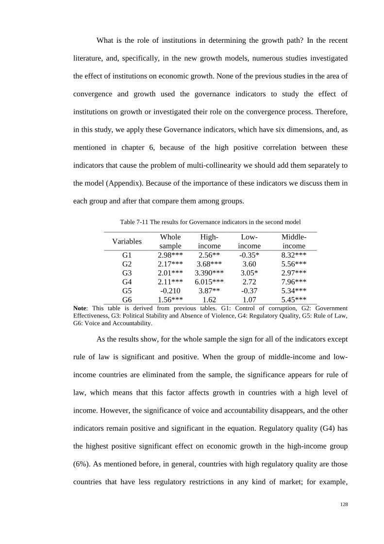
128
What is the role of institutions in determining the growth path? In the recent
literature, and, specifically, in the new growth models, numerous studies investigated
the effect of institutions on economic growth. None of the previous studies in the area of
convergence and growth used the governance indicators to study the effect of
institutions on growth or investigated their role on the convergence process. Therefore,
in this study, we apply these Governance indicators, which have six dimensions, and, as
mentioned in chapter 6, because of the high positive correlation between these
indicators that cause the problem of multi-collinearity we should add them separately to
the model (Appendix). Because of the importance of these indicators we discuss them in
each group and after that compare them among groups.
Table 7-11 The results for Governance indicators in the second model
Variables Whole
sample
High-
income
Low-
income
Middle-
income
G1 2.98*** 2.56** -0.35* 8.32***
G2 2.17*** 3.68*** 3.60 5.56***
G3 2.01*** 3.390*** 3.05* 2.97***
G4 2.11*** 6.015*** 2.72 7.96***
G5 -0.210 3.87** -0.37 5.34***
G6 1.56*** 1.62 1.07 5.45*** Note: This table is derived from previous tables. G1: Control of corruption, G2: Government
Effectiveness, G3: Political Stability and Absence of Violence, G4: Regulatory Quality, G5: Rule of Law,
G6: Voice and Accountability.
As the results show, for the whole sample the sign for all of the indicators except
rule of law is significant and positive. When the group of middle-income and low-
income countries are eliminated from the sample, the significance appears for rule of
law, which means that this factor affects growth in countries with a high level of
income. However, the significance of voice and accountability disappears, and the other
indicators remain positive and significant in the equation. Regulatory quality (G4) has
the highest positive significant effect on economic growth in the high-income group
(6%). As mentioned before, in general, countries with high regulatory quality are those
countries that have less regulatory restrictions in any kind of market; for example,
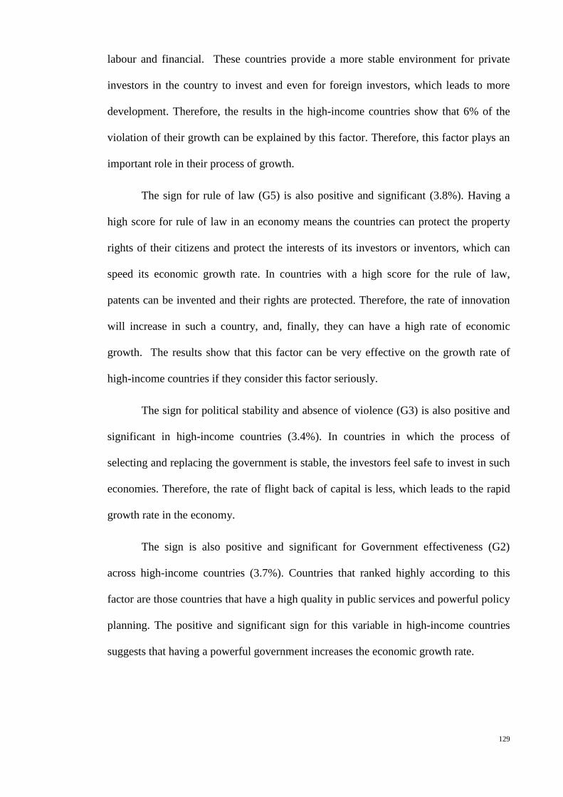
129
labour and financial. These countries provide a more stable environment for private
investors in the country to invest and even for foreign investors, which leads to more
development. Therefore, the results in the high-income countries show that 6% of the
violation of their growth can be explained by this factor. Therefore, this factor plays an
important role in their process of growth.
The sign for rule of law (G5) is also positive and significant (3.8%). Having a
high score for rule of law in an economy means the countries can protect the property
rights of their citizens and protect the interests of its investors or inventors, which can
speed its economic growth rate. In countries with a high score for the rule of law,
patents can be invented and their rights are protected. Therefore, the rate of innovation
will increase in such a country, and, finally, they can have a high rate of economic
growth. The results show that this factor can be very effective on the growth rate of
high-income countries if they consider this factor seriously.
The sign for political stability and absence of violence (G3) is also positive and
significant in high-income countries (3.4%). In countries in which the process of
selecting and replacing the government is stable, the investors feel safe to invest in such
economies. Therefore, the rate of flight back of capital is less, which leads to the rapid
growth rate in the economy.
The sign is also positive and significant for Government effectiveness (G2)
across high-income countries (3.7%). Countries that ranked highly according to this
factor are those countries that have a high quality in public services and powerful policy
planning. The positive and significant sign for this variable in high-income countries
suggests that having a powerful government increases the economic growth rate.

130
The sign for control of corruption (G1) is also positive and significant across
high-income countries (2.56%), which show that developed countries with a high
control of corruption are successful in giving confidence to the investors to invest in the
economy.
Finally, the results show that the only factor that is not significant across high-
income countries for economic growth is voice and accountability (G6). This means that
the productivity of a country is not affected by the system in which the government is
selected. In the other words, the other reason could be that all these high-income
countries have strong voice and accountability indicators, so there is not much variation
in this indicator to explain growth.
For middle-income countries the results show that for all of the indicators the
signs are positive and significantly different from zero, and also stronger than for high-
income countries. Among all the indicators, control of corruption (G1) has the highest
positive significant effect on economic growth in the middle-income group. This shows
that by controlling their corruption developing countries can be successful in giving
confidence to the investors to invest in their economy and thereby grow fast (8.3% of
the variation is explained by this factor).
The regulatory quality (G4) is the second highest positive significant effective
factor on economic growth (7.96%). These countries, by providing a safe environment
for private investors and foreign investors can increase their productivity.
The sign is also positive and significant for government effectiveness (G2)
across high-income countries (5.56%). The results suggest that having a powerful
government increases the economic growth rate across developing countries.

131
The results for voice and accountability (G6) are positive and significantly
different from zero, thereby indicating that the productivity of a country is affected by
the system in which government is selected across developing countries. This result
contradicts the result of high-income countries where the voice and accountability did
not affect the growth rate of the high-income countries.
The sign for rule of law (G5) is also positive and significant (5.35%). This
shows that building a strong system of justice and law for protecting the rights of the
citizens will be effective for growth.
The sign for political stability and absence of violence (G3) is also positive and
significant in middle-income countries (2.9%). In countries in which the process of
selecting and replacing government is stable, the investors feel safer to invest in such
economies. Therefore, the rate of flight back of capital is less and leads to a rapid
growth rate in the economy.
However, for low-income countries the significance disappears for almost all of
the factors controlling for corruption for which the sign is negative and significant at
10%. This is an interesting result for two reasons. First, because again it raises the issue
of the income threshold. Our explanation for this result is that since these countries do
not reach a certain level of income and development, they cannot take advantage of
these factors. Second, as we said, the sign of control for corruption is negative in this
group, meaning that controlling for corruption is not effective in low-income countries.
The issue of corruption and level of development is a big issue in recent literature. Some
economists believe we can track developed countries and see that they are not fighting
corruption in the initial stages of their development (Khan, 2004). Khan (2004) argues
that fighting corruption, though necessary, is not the only prerequisite for growth. This
itself is further support for reaching the income threshold. In the other research Mironov

132
(2005) analyses the effects of corruption on economic growth across 141 countries
during 1996 and 2004. The results of his study are another support for what the current
research found. His results show that residual corruption has positive effects on
economic growth. In other words, he found out that the residual corruption is correlated
positively with capital accumulation and so economic growth in developing countries
and poor countries. Furthermore, Heckelman and Powell (2008) in another research
show that limiting economic freedom causes the corruption to have a positive effect on
economic growth.
7.2.3 δ - Convergence
“δ convergence” means that the dispersion of GDP per capita reduces over time. There
exist several ways of quantifying the inequality of income distributions but a commonly
used measure is the standard deviation of the logarithms of per capita GDP. If the value
of standard deviation in a sample becomes smaller it means that the country reduced the
gap that existed. Otherwise, there is no δ convergence. Table 7-12 shows the results of
the analysis of δ convergence for GDP per capita in the following groups of countries.
Table 7-12 Results of testing δ convergence in terms of GDP per capita, 1996-2010
GDP per capita
Coefficient of
variation in t96
Coefficient of
variation in t2010
Rate of change (%)
High-income 0.898552 0.805812 -10.321
Middle-income ( upper ) 0.668754 0.522679 -21.8429
Middle-income ( lower ) 0.620489 0.539005 -13.1323
Low-income 0.54205 0.491879 -9.25579
Note: Standard deviation of logarithms of GDP per capita,1996-2010, Rate of changes=( t2010-t96/t96)*100

133
The results show that in all three groups of countries there is a decreasing
dispersion in terms of GDP per capita across countries over time. However, the speed of
δ convergence is rapid in upper middle-income countries. The lowest rate belongs to the
low-income countries, which is 9 per cent. This result is exactly in line with our β
convergence in which the rate of convergence is particularly rapid for the middle-
income group.
7.3 New Growth Model
In this section, we are going to test β Convergence and φ Convergence by
applying the dynamic system GMM across groups of sample countries. As can be seen
the concept of β Convergence is the same as the neoclassic model, meaning that if the
sign of initial GDP per capita is negative countries behind the steady state can grow
faster, otherwise there is divergence across countries. What makes this model different
from the NCGM is the way that the variables apply in the model. As we described in
chapter 3, we focused on the new growth models where, in these models, technology
plays an important role in explaining the different growth rate across countries unlike
the NCG model where the emphasis was on capital accumulation. We expect the sign
for innovation, globalization and institutions to be more sensitive than capital
accumulation in these classes of models in our sample.

134
7.3.1 Testing β Convergence: The Link Between Technological Change and
Convergence in Income
In chapter three we showed how we link technology change and growth of GDP
per capita in terms of endogenous theories. This section presents the results of
estimating the following equation:
∆𝑦𝑖,𝑡𝑦𝑖,𝑡
⁄ = 𝜃1𝑙𝑜𝑔𝐼𝑁𝑂𝑖,𝑡 + 𝜃2𝑙𝑜𝑔𝐻𝐶𝑖,𝑡 + 𝜃3𝑙𝑜𝑔𝐼𝑁𝑆𝑖,𝑡 + 𝜃4𝑙𝑜𝑔𝐺𝐿𝑂𝐵𝑖,𝑡 + 𝜃5𝐹𝐶𝑖,𝑡 +
𝜇log𝑦𝑖,𝑡−1 −ζ𝑡 + 𝜌𝑖 + 휀𝑖,𝑡 (7-3)
Where ∆𝑙𝑜𝑔𝑦𝑖,𝑡 ,growth rate of GDP per capita at time (t), is related to log𝑦𝑖,𝑡−1
,the logarithm of GDP per capita at the start of the period, and other controlling
variables, such as physical capital accumulation, the intensity of innovation activities,
human capital level, the institutions (governance indicators) and globalization. By
estimating this equation we can understand how much of the growth can be explained
by technological changes and how much by physical accumulation. The coefficient of
log𝑦𝑖,𝑡−1 shows whether convergence happened across countries or not. If it is negative,
it means that countries behind the steady state can grow faster, otherwise there is
divergence across countries.
β convergence is tested by applying equation (7-3) in samples of low-income,
middle-income and high-income countries between 1996 and 2010 in terms of GDP per
capita based on the new growth theory. All the variables are taken in natural log form.
The country specific effects are controlled by following the generalized method of
moment’s estimation procedure. Tables 7-13, 7-14, 7-15 and 7-16 show the results of
testing β convergence for the whole sample as well as for high-income, middle-income
and low-income countries:
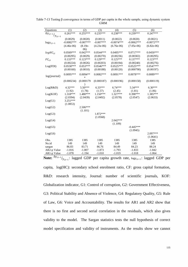
135
Table 7-13 Testing β convergence in terms of GDP per capita in the whole sample, using dynamic system
GMM
Equations (1) (2) (3) (4) (5) (6) ∆𝑦𝑖,𝑡−1
𝑦𝑖,𝑡−1⁄
0.261*** 0.255*** 0.235*** 0.238*** 0.239*** 0.247***
(0.0029) (0.0020) (0.0011) (0.0022) (0.0020) (0.0021)
log𝑦𝑖,𝑡−1 -0.0082*** -0.007*** -0.007*** -0.0074*** -0.0062*** -0.0072***
(4.46e-06) (8.19e-
06)
(4.23e-06) (6.76e-06) (7.05e-06) (6.82e-06)
𝑙𝑜𝑔𝐻𝐶𝑖,𝑡 0.0569*** 0.042*** 0.0544*** 0.0495*** 0.0717*** 0.0450***
(0.00295) (0.0029) (0.00270) (0.00236) (0.00302) (0.00295)
𝐹𝐶𝑖,𝑡 0.133*** 0.123*** 0.129*** 0.125*** 0.137*** 0.123***
(0.00224) (0.0026) (0.00203) (0.00194) (0.00240) (0.00276)
Log(FDI) 0.0558*** 0.053*** 0.0546*** 0.0525*** 0.0525*** 0.0547***
(0.00160) (0.0010) (0.00188) (0.00120) (0.000790) (0.00197)
log (journal) 0.0095*** 0.0094**
*
0.0082*** 0.0091*** 0.0078*** 0.0089***
(0.000234) (0.000179
)
(0.000187) (0.000196) (0.000158) (0.000119)
Log(R&D) 4.32*** 5.50*** 6.33*** 6.74*** 5.34*** 6.30***
(1.92) (1.78) (1.57) (2.45) (1.81) (1.06)
Log(KOF) 1.318*** 1.480*** 1.150*** 1.327*** 0.398*** 1.385***
(2.0394) (2.0439) (2.0492) (2.0578) (2.0547) (2.0633)
Log(G1) 3.251***
(1.0853)
Log(G2) 2.506***
(1.101)
Log(G3) 1.872***
(1.0568)
Log(G4) 2.042***
(1.109)
Log(G5) -0.445***
(1.0945)
Log(G6) 2.097***
(1.0641)
Obs. 1385 1385 1385 1385 1385 1385
No.id 149 149 149 149 149 149
sargan 86.83 83.71 86.76 84.49 84.23 88.24
AR2-p Value -1.816 -1.807 -1.873 -1.793 -1.833 -1.842
AR1-p Value -1.078 -1.194 -1.010 -1.019 -1.018 -1.064
Note: ∆yi,t−1
yi,t−1⁄ : lagged GDP per capita growth rate, logyi,t−1 : lagged GDP per
capita, log(HC): secondary school enrolment ratio, CF: gross capital formation,
R&D: research intensity, Journal: number of scientific journals, KOF:
Globalization indicator, G1: Control of corruption, G2: Government Effectiveness,
G3: Political Stability and Absence of Violence, G4: Regulatory Quality, G5: Rule
of Law, G6: Voice and Accountability. The results for AR1 and AR2 show that
there is no first and second serial correlation in the residuals, which also gives
validity to the model. The Sargan statistics tests the null hypothesis of correct
model specification and validity of instruments. As the results show we cannot

136
reject the null hypothesis, which shows that, the instruments are valid. Time
dummies are also included, which is not reported here.
137
Table 7-14 Testing β convergence in terms of GDP per capita using dynamic System GMM across High
income countries
Equations (1) (2) (3) (4) (5) (6) ∆𝑦𝑖,𝑡−1
𝑦𝑖,𝑡−1⁄ 0.644*** 0.617*** 0.637*** 0.619*** 0.643*** 0.659***
(0.0931) (0.0920) (0.0946) (0.0922) (0.0940) (0.0933)
log𝑦𝑖,𝑡−1 -0.45* -0.488* -0.455** -1 -0.474** -0.46*
(0.085) (0.011) (0.950) (0.000) (0.247) (0.063)
𝑙𝑜𝑔𝐻𝐶𝑖,𝑡 -15.91 -12.10 -20.36 12.94 17.14** 14.75*
(5.258) (5.435) (5.076) (5.409) (5.454) (5.168)
𝐹𝐶𝑖,𝑡 0.520*** 0.529*** 0.558*** 0.527*** 0.544*** 0.564***
(0.0549) (0.0802) (0.0574) (0.0681) (0.0717) (0.0607)
Log(FDI) 1.729*** 2.791*** 2.508** 2.739*** 2.520** 1.288
(1.234) 1.226) (1.249) 1.222) 1.216) (0.209)
log (journal) 1.0776*** 1.0798**
*
1.0839*** 1.0907*** 1.0809*** 0.9669***
(1.00993) (1.0134) (1.0145) (1.0139) (1.0132) (1.0123)
Log(R&D) 6.0484*** 6.0510**
*
6.0489*** 6.0540*** 5.0501*** 6.0446***
(1. 468) (1. 0317) (1. 305) (1. 364) (1. 504) (1. 489)
Log(KOF) 4.038* 4.608** 4.303** 4.515** 4.311* 4.353**
(3.123) (1.112) (1.138) (2.781) (1.117) (1.222)
Log(G1) 2.386***
(1.532)
Log(G2) 4.364***
(1.666)
Log(G3) 4.271**
(1.485)
Log(G4) 7.770***
(1.127)
Log(G5) 3.264*
(0.866)
Log(G6) 1.502***
(1.125)
sargan 207.79408 207.7880 209.07359 208.94014 209.60235 199.03852
AR2-p Value .31235034 .4591524 .26509498 .29570693 .28689714 .90706144
AR1-p Value .10597 .1408266
5 .11226635 .1434355 .12020117 .09581717
Obs. 379 379 379 379 379 379
No.id 29 29 29 29 29 29
Note: ∆yi,t−1
yi,t−1⁄ : lagged GDP per capita growth rate, 𝑙𝑜𝑔yi,t−1 : lagged GDP per
capita, log(HC): secondary school enrolment ratio, CF: gross capital formation,
R&D: research intensity, Journal: number of scientific journals, KOF:
Globalization indicator, G1: Control of corruption, G2: Government Effectiveness,
G3: Political Stability and Absence of Violence, G4: Regulatory Quality, G5: Rule
of Law, G6: Voice and Accountability. The results for AR1 and AR2 show that
there is no first and second serial correlation in the residuals which also give
validity to the model. The Sargan statistics tests the null hypothesis of correct
model specification and validity of instruments. As the results show we cannot

138
reject the null hypothesis, which shows that the instruments are valid. Time
dummies are also included, which is not reported here.

139
Table 7-15 Dynamic system GMM, testing β convergence in terms of GDP in middle-income countries.
Equations (1) (2) (3) (4) (5) (6) ∆𝑦𝑖,𝑡−1
𝑦𝑖,𝑡−1⁄ 0.674*** 0.669*** 0.653*** 0.649*** 0.652*** 0.651***
(0.0976) (0.0981) (0.0964) (0.0956) (0.0973) (0.0980)
log𝑦𝑖,𝑡−1 -0.648*** -0.723*** -0.762*** -0.68*** -0.848*** -0.732**
(1.024) (0.961) (0.932) (0.919) (0.959) (0.929)
𝑙𝑜𝑔𝐻𝐶𝑖,𝑡 0.930 0.519 -0.0806 0.978 0.772 0.728
(2.362) (2.374) (2.507) (2.391) (2.367) (2.357)
𝐹𝐶𝑖,𝑡 0.318* 0.154** 0.255* 0.115** 0.0720*** 0.134**
(1.749) (1.745) (1.735) (1.717) (1.734) (1.731)
Log(FDI) 3.59*** 1.99*** 3.86*** 3.87*** 2.33*** 2.91***
(8.02e-07) (7.31e-
07)
(9.21e-07) (5.97e-07) (4.87e-07) (8.78e-07)
log (journal) 1. 014** 1. 029*** 1. 0558** 1. 0798** 1. 044** 1. 015*
(0. 168) (0. 102) (0. 286) (0. 217) (0. 153) (0. 344)
Log(R&D) 5.238** 5.455** 5.337** 5.937** 5.584** 5.0543**
(1.590) (1.630) (1.686) (1.466) (1.578) (1.572)
Log(KOF) 9. 234*** 8. 41*** 8. 618*** 8. 661*** 8. 426** 8. 415***
(10. 818) (1. 638) (1. 850) (1. 170) (1. 180) (1. 797)
Log(G1) 4.181*
(0.956)
Log(G2) 4.513**
(0.921)
Log(G3) 7.621**
(0.839)
Log(G4) 6.806**
(0.887)
Log(G5) -4.557
(0.886)
Log(G6) 5.503*
(0.953)
sargan 165.48596 166.5270 168.9306 170.72275 168.59732 169.10407
AR2-p Value .2696833 .2667295 .25331787 .25700299 .26083871 .2596185
AR1-p Value .23076397 .2047918 .21083427 .26090361 .23084908 .20482335
Obs. 456 456 456 456 456 456
No.id 90 90 90 90 90 90
Note: ∆yi,t−1
yi,t−1⁄ : lagged GDP per capita growth rate, 𝑙𝑜𝑔yi,t−1 : lagged GDP per
capita, log(HC): secondary school enrolment ratio, CF: gross capital formation,
R&D: research intensity, Journal: number of scientific journals, KOF:
Globalization indicator, G1: Control of corruption, G2: Government Effectiveness,
G3: Political Stability and Absence of Violence, G4: Regulatory Quality, G5: Rule
of Law, G6: Voice and Accountability. The results for AR1 and AR2 show that
there is no first and second serial correlation in the residuals which also give
validity to the model. The Sargan statistics tests the null hypothesis of correct
model specification and validity of instruments. As the results show we cannot
reject the null hypothesis, which shows that the instruments are valid. Time
dummies are also included, which is not reported here.

140
Table 7-16 Testing β convergence in terms of GDP in low-income countries, Using dynamic system
GMM.
Equations (1) (2) (3) (4) (5) (6) ∆𝑦𝑖,𝑡−1
𝑦𝑖,𝑡−1⁄ 0.224 0.191 0.211 0.213 0.203 0.198
(0.264) (0.268) (0.263) (0.267) (0.268) (0.262)
log𝑦𝑖,𝑡−1 -0.0289*** -
0.0283**
*
-0.0295*** -0.0323*** -0.0277*** -0.0302***
(0.102) (0.960) (0.093) (0.007) 0.909) (0.072)
𝑙𝑜𝑔𝐻𝐶𝑖,𝑡 3.415*** 2.338** 3.217*** 2.520*** 2.629*** 2.620***
(2.078) (1.727) (1.716) (2.045) (1.758) (1.576)
𝐹𝐶𝑖,𝑡 3.0530** 3.750*** 3.0313*** 3.529*** 3.202** 3.357**
(2.051) (2.287) (2.082) (2.432) (2.118) (2.106)
Log(FDI) 1.592 2.021 0.899* 1.216 0.165 1.433
(6.826) (6.148) (0.871) (6.053) (0.088) (5.893)
log (journal) 0.635 -0.293 0.522 0.326* 0.416 0.441
(0.912) (0.984) (0.974) (1.139) (0.986) (0.915)
Log(R&D) 0.734 -1.284 -0.413 0.00503 -0.411 1.146
(4.570) (4.740) (0.860) (0.008) (0.702) (4.640)
Log(KOF) 0.0726 0.0314 0.0494 0.0721 0.0185 0.0477
(0.0693) (0.0621) (0.0743) (0.0677) (0.0468) (0.0674)
Log(G1) -0.575
(0.555)
Log(G2) 3.885
(5.268)
Log(G3) -0.229
(0.521)
Log(G4) -0.993
(0.670)
Log(G5) 1.349
(3.206)
Log(G6) -1.204
(2.014)
sargan 22.370168 20.42315 22.151908 21.017792 21.099152 21.690762
AR2-p Value .15293232 .1887076 .13746631 .29462389 .18951612 .277408
AR1-p Value .43416257 .4610631 .41256745 .24585619 .33327424 .11344095
Obs. 198 198 198 198 198 198
No.id 30 30 30 30 30 30
Note: ∆yi,t−1
yi,t−1⁄ : lagged GDP per capita growth rate, 𝑙𝑜𝑔yi,t−1 : lagged GDP per
capita, log(HC): secondary school enrolment ratio, CF: gross capital formation,
R&D: research intensity, Journal: number of scientific journals, KOF:
Globalization indicator, G1: Control of corruption, G2: Government Effectiveness,
G3: Political Stability and Absence of Violence, G4: Regulatory Quality, G5: Rule
of Law, G6: Voice and Accountability. The results for AR1 and AR2 show that
there is no first and second serial correlation in the residuals which also give
validity to the model. The Sargan statistics tests the null hypothesis of correct
model specification and validity of instruments. As the results show we cannot
reject the null hypothesis, which shows that the instruments are valid. Time
dummies are also included, which is not reported here.

141

142
As can be seen, we have six equations estimated in each table and in each equation
a different governance indicator is entered to be tested. First, we analyse the speed of
convergence in each group separately. Table 7-17 shows the implied speed of
convergence, which is calculated like before:
Table 7-17 Speed of Convergence in New Growth model, 1996-2010
Countries Eq 1 2 3 4 5 6
Whole
sample
Initial GDP per
capita coefficient
-
0.00828*
**
-
0.00772*
**
-
0.00702*
**
-
0.00741*
**
-
0.00623*
**
-
0.00725*
**
𝜆 =Speed of
convergence 0.000554 0.000517 0.00047 0.000496
0.000416
6 0.000485
1
High-
income
Initial GDP per
capita coefficient -0.45 -0.488 -0.55 -1 -0.474 -0.46
𝜆 =Speed of
convergence 0.039856
0.044628
7 0.053234 …… 0.04283
0.041079
1
Middle
-
income
Initial GDP per
capita coefficient
-
0.648***
-
0.723***
-
0.762*** -0.68***
-
0.848*** -0.732**
𝜆 =Speed of
convergence
0.069608
3
0.085582
5 0.095699 0.075962
0.125591
7
0.087784
6
Low-
income
Initial GDP per
capita coefficient -
0.0289*** -
0.0283*** -
0.0295*** -
0.0323*** -
0.0277*** -
0.0302***
𝜆 =Speed of
convergence 0.00195 0.00191 0.00199 0.00218 0.00187 0.00204
Note: the first row of each group reports the coefficient of initial GDP per capita in each equation
separately. The second row shows the speed of convergence related to each equation.
For the whole sample, as well as the split samples we can see that the
convergence is similar to the neoclassical growth model. The coefficient of initial GDP
per capita is negative, meaning that countries far from the steady state growth path can
grow faster. It is interesting when we compare the result with the NCGM. As can be
seen, for high-income countries, on average, almost 4% of the gap between the initial
level of GDP per capita and the repetitive steady state vanishes in one year, which is
higher than the result of the NCGM, which was 3%.
For middle-income countries, on average, almost 9% of the gap between the
initial level of GDP per capita and the repetitive steady state vanishes in one year. Again
the results of NGM show the faster convergence compared to NCGM, which was 8%.

143
Finally, for low-income countries less than 1% of the gap between the initial
level of GDP per capita and the repetitive steady state vanishes in one year. This result
is slower than the NCG model, which was 1%.
To sum up, comparing the results of NGM with NCGM, the rate of convergence
for both high-income and middle-income countries is higher in the new growth model
than the neoclassical growth model. However, for the low-income countries it is slower.
Our explanation for this result is that since the middle-income and high-income
countries have the capacity to take advantage of the technology of the frontiers, the
explanatory variables that were added to the model to determine the steady state of
growth path across these countries are effective on GDP growth, and, hence, accelerate
the convergence process. This is consistent with the notion of the new growth theory in
which technological change is the main source of growth. As discussed before in this
study, the explanatory variables, in new growth regression, are components of
productivity growth and through the channel of technology they affect GDP growth, so
we can see that through this channel they are more effective on GDP growth across
those countries that are developed or in the later stages of development. The set of
results for low-income countries is another proof of this, since these countries are
undeveloped or in the early stages of development these factors through the channel of
technology are not effective on them. Therefore, the NCG model is the model that
should apply for these countries with this level of income. In other words we can say
that selecting which growth model should be applied for countries is monotonic to their
income level, whether capital deepening models or technological catching up models. In
other words, an income threshold may need to be reached before countries can take
advantage of technological change. Countries below that threshold are caught in a
poverty trap from which it takes a long time to escape.
144
7.3.1.1 Determinants of Growth in the New Growth Model
Tables (7-8),(7-9), (7-10) and (7-11) also report the effects of investing in
human capital, physical capital, globalization indicators, FDI and KOF index,
institutions factor, R&D intensity and number of scientific journals on economic growth
across these groups of countries. Once again, it is necessary to emphasize the
differences between this model and the NCGM. In the NGM all these factors except
physical capital, affect technology, and, through the channel of technology, they affect
economic growth, while in the NCGM, innovation, globalization and institutions are the
factors that facilitate human capital accumulation in the process of growth.
If we take a look at the signs and significance of the variables in the new growth
regression in the middle-income and high-income countries it is clear that they are
stronger and more effective than in the NCG regression.
As can be seen, the sign of secondary school enrolment ratio is negative and not
significant in most of the equations across high-income countries. Secondary education,
while an important building block, cannot capture this skill level, given that it would be
universal in all high-income countries. The sign of secondary school enrolment ratio is
positive but not significant across middle-income countries as well. However, the sign is
positive and significant in low-income countries and very significant. This means that
by investing more in their secondary education level, low-income countries can speed
their economic growth.
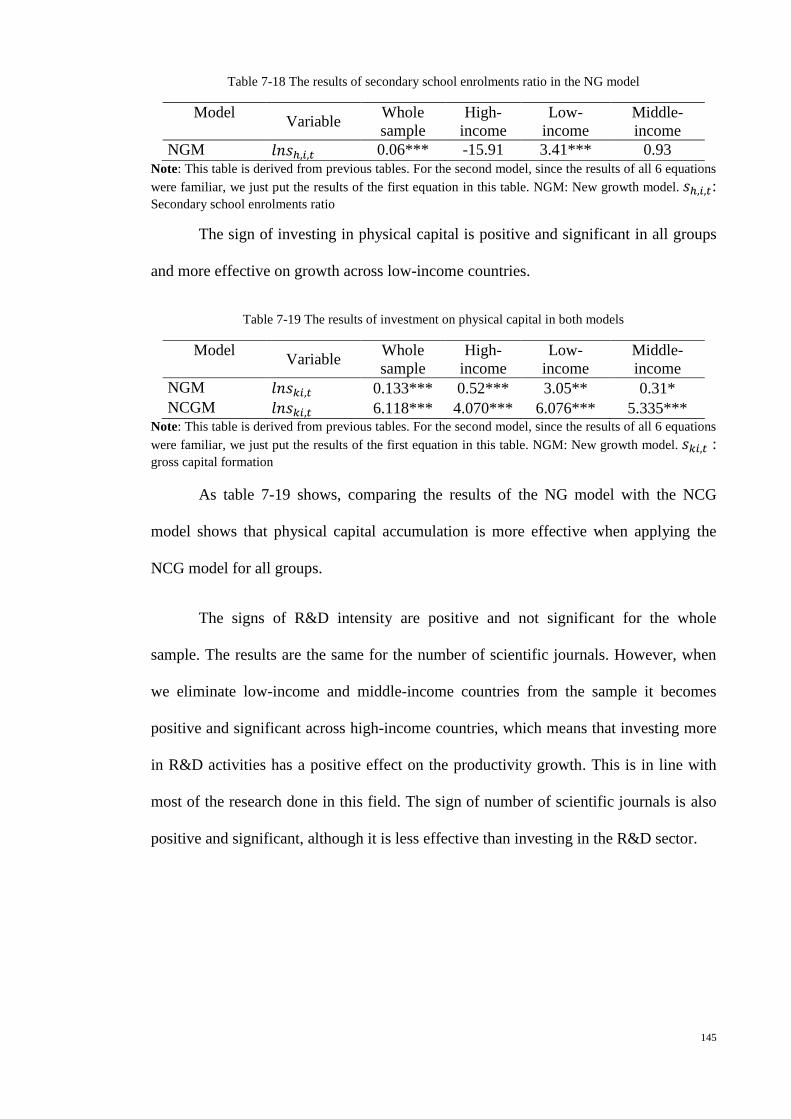
145
Table 7-18 The results of secondary school enrolments ratio in the NG model
Model Variable
Whole
sample
High-
income
Low-
income
Middle-
income
NGM 𝑙𝑛𝑠ℎ,𝑖,𝑡 0.06*** -15.91 3.41*** 0.93
Note: This table is derived from previous tables. For the second model, since the results of all 6 equations
were familiar, we just put the results of the first equation in this table. NGM: New growth model. 𝑠ℎ,𝑖,𝑡: Secondary school enrolments ratio
The sign of investing in physical capital is positive and significant in all groups
and more effective on growth across low-income countries.
Table 7-19 The results of investment on physical capital in both models
Model Variable
Whole
sample
High-
income
Low-
income
Middle-
income
NGM 𝑙𝑛𝑠𝑘𝑖,𝑡 0.133*** 0.52*** 3.05** 0.31*
NCGM 𝑙𝑛𝑠𝑘𝑖,𝑡 6.118*** 4.070*** 6.076*** 5.335*** Note: This table is derived from previous tables. For the second model, since the results of all 6 equations
were familiar, we just put the results of the first equation in this table. NGM: New growth model. 𝑠𝑘𝑖,𝑡 : gross capital formation
As table 7-19 shows, comparing the results of the NG model with the NCG
model shows that physical capital accumulation is more effective when applying the
NCG model for all groups.
The signs of R&D intensity are positive and not significant for the whole
sample. The results are the same for the number of scientific journals. However, when
we eliminate low-income and middle-income countries from the sample it becomes
positive and significant across high-income countries, which means that investing more
in R&D activities has a positive effect on the productivity growth. This is in line with
most of the research done in this field. The sign of number of scientific journals is also
positive and significant, although it is less effective than investing in the R&D sector.

146
Table 7-20 The results of R&D intensity and Number of scientific Journals in both models
Whole sample High-income Low-income Middle-income
NCG NG NCG NG NCG NG NCG NG
R&D 3.88*** 4.32*** 5.50** 6.04*** 0.01* 0.73 4.96*** 5.23**
No.Jour
nals
-0.01** 0.001*** 0.538*** 1.07*** -0.0002 0.63 0.95** 1.01***
Note: This table is derived from previous tables. For the second model, since the results of all 6 equations
were familiar, we just put the results of the first equation in this table. NG: New growth model. NCG:
Neoclassical growth model.
The results of R&D intensity are also positive and significant for middle-income
countries, which mean that by considering technology transfer they can take advantage
from the output of R&D activities. Comparing the results of R&D intensity with the
NCG model shows that R&D intensity is more effective on growth in the NG model
than in the NCG model. The sign of number of scientific journals is positive and
significant in this group.
For low-income countries, as can be seen, the signs of R&D intensity and
number of scientific journals are positive but not significant in most equations. We have
the same explanation as for the neoclassical growth theory: investing more in R&D
activities is not working since they do not have an adequate level of human capital or
sufficient highly skilled workers to take advantage of the outcomes of R&D activities.
For high-income countries, the effect of the KOF index is positive and
significant and more effective than the NCG model. This means that globalization can
increase economic growth across countries with a high level of income. The sign of FDI
is also positive and significant in this group but less effective than the KOF index.
Again this could be a good sign that this new KOF index is a better proxy for measuring
globalization, as it not only measures the flow of goods, but also the flow of technology
and knowledge by considering the infrastructures, such as Internet users and telephone
lines.

147
Table 7-21 The results of the KOF index and FDI in both models
Whole sample High-income Low-income Middle-income
NCG NG NCG NG NCG NG NCG NG
KOF 4.27*** 1.31*** 3.1*** 4.60** 9.03*** 0.072 7.19*** 9.23***
FDI 0.05*** 0.05*** 0.97*** 1.72*** 0.07** 1.59 0.02** 3.59***
Note: This table is derived from previous tables. For the second model, since the results of all 6 equations
were familiar, we just put the results of the first equation in this table. NG: New growth model. NCG:
Neoclassical growth model.
For middle-income countries the results for both variables are the same, and
these countries can also take advantage of international technology spillovers through
globalization since they have a high enough level of human capital in their countries.
Again the results are more effective than the NCG model.
The story is different for low-income countries. Neither the KOF index nor the
FDI has a significant effect on economic growth in this model. However, as can be seen,
the results were significant for the NCG model. One explanation for this might be that
since we apply these variables in NGM through the channel of technology, and as
components of technology regression, they are not effective in countries with a low
level of income or those countries that are not yet developed. This leads to the
interpretation that the application of each class of growth model is dependent on the
level of development. For example, in high-income countries where there is a sufficient
level of human capital, technology spillovers through globalization and innovation are
effective, whereas, when considering low-income countries with underdeveloped
economies, these factors are no longer effective.
Governance indicators have a positive and significant effect on economic growth
across high-income countries, and, as can be seen, they are more effective than the NCG
model. For middle-income countries, except for the rule of law, the other governance
indicators have a positive and significant effect on economic growth and are more
effective than the NCG model on GDP growth. For low-income countries, none of the
governance indicators are significant.
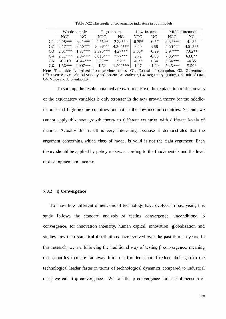
148
Table 7-22 The results of Governance indicators in both models
Whole sample High-income Low-income Middle-income
NCG NG NCG NG NCG NG NCG NG
G1 2.98*** 3.21*** 2.56** 2.38*** -0.35* -0.57 8.32*** 4.18*
G2 2.17*** 2.50*** 3.68*** 4.364*** 3.60 3.88 5.56*** 4.513**
G3 2.01*** 1.87*** 3.390*** 4.27*** 3.05* -0.29 2.97*** 7.62**
G4 2.11*** 2.04*** 6.015*** 7.77*** 2.72 -0.99 7.96*** 6.80**
G5 -0.210 -0.44*** 3.87** 3.26* -0.37 1.34 5.34*** -4.55
G6 1.56*** 2.097*** 1.62 1.502*** 1.07 -1.20 5.45*** 5.50* Note: This table is derived from previous tables. G1: Control of corruption, G2: Government
Effectiveness, G3: Political Stability and Absence of Violence, G4: Regulatory Quality, G5: Rule of Law,
G6: Voice and Accountability.
To sum up, the results obtained are two-fold. First, the explanation of the powers
of the explanatory variables is only stronger in the new growth theory for the middle-
income and high-income countries but not in the low-income countries. Second, we
cannot apply this new growth theory to different countries with different levels of
income. Actually this result is very interesting, because it demonstrates that the
argument concerning which class of model is valid is not the right argument. Each
theory should be applied by policy makers according to the fundamentals and the level
of development and income.
7.3.2 φ Convergence
To show how different dimensions of technology have evolved in past years, this
study follows the standard analysis of testing convergence, unconditional β
convergence, for innovation intensity, human capital, innovation, globalization and
studies how their statistical distributions have evolved over the past thirteen years. In
this research, we are following the traditional way of testing β convergence, meaning
that countries that are far away from the frontiers should reduce their gap to the
technological leader faster in terms of technological dynamics compared to industrial
ones; we call it φ convergence. We test the φ convergence for each dimension of

149
technology over the period 1996-2010 to see the new aspects that can affect the
distribution of technological activities in the world (Castellacci, 2011):
1- Governance indicators (6 indicators for institutions)
2- KOF index and FDI index (proxy of Globalization)
3- R&D intensity and number of scientific journals (proxy for innovation)
4- Secondary school enrolment (proxy for human capital)
Using exactly the same method that is used by R. Barro and Sala-i-Martin (1995) for
testing the β convergence, the initial level of each variable is used as the only regressor
and the annual growth rate of each dimension is the dependent variable.
∆𝐴𝑖𝐴𝑖
⁄ = 𝛼 + 𝜑1𝐴𝑖,0 + 휀𝑖 (7-2)
Where ∆𝐴𝑖
𝐴𝑖⁄ is the growth rate for each technology dimension of country i
over the period 1996-2010, and 𝐴𝑖,0 is the the log of its initial level at the beginning of
the period. 𝜑1shows the speed of convergence for each dimension of technology. Table
7-23 shows the results.
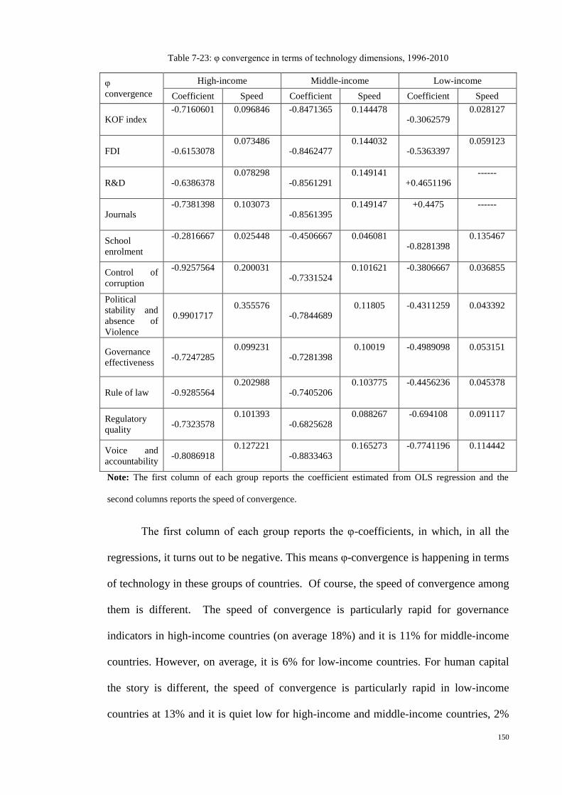
150
Table 7-23: φ convergence in terms of technology dimensions, 1996-2010
φ
convergence
High-income Middle-income Low-income
Coefficient Speed Coefficient Speed Coefficient Speed
KOF index -0.7160601 0.096846 -0.8471365 0.144478
-0.3062579 0.028127
FDI -0.6153078 0.073486
-0.8462477 0.144032
-0.5363397 0.059123
R&D -0.6386378 0.078298
-0.8561291 0.149141
+0.4651196 ------
Journals -0.7381398 0.103073
-0.8561395 0.149147 +0.4475 ------
School
enrolment
-0.2816667 0.025448 -0.4506667 0.046081 -0.8281398
0.135467
Control of
corruption
-0.9257564 0.200031 -0.7331524
0.101621 -0.3806667 0.036855
Political
stability and
absence of
Violence
0.9901717 0.355576
-0.7844689 0.11805 -0.4311259 0.043392
Governance
effectiveness -0.7247285
0.099231 -0.7281398
0.10019 -0.4989098 0.053151
Rule of law -0.9285564 0.202988
-0.7405206 0.103775 -0.4456236 0.045378
Regulatory
quality -0.7323578
0.101393 -0.6825628
0.088267 -0.694108 0.091117
Voice and
accountability -0.8086918
0.127221 -0.8833463
0.165273 -0.7741196 0.114442
Note: The first column of each group reports the coefficient estimated from OLS regression and the
second columns reports the speed of convergence.
The first column of each group reports the φ-coefficients, in which, in all the
regressions, it turns out to be negative. This means φ-convergence is happening in terms
of technology in these groups of countries. Of course, the speed of convergence among
them is different. The speed of convergence is particularly rapid for governance
indicators in high-income countries (on average 18%) and it is 11% for middle-income
countries. However, on average, it is 6% for low-income countries. For human capital
the story is different, the speed of convergence is particularly rapid in low-income
countries at 13% and it is quiet low for high-income and middle-income countries, 2%

151
and 4%, respectively. This is consistent with the idea of M. R. Islam (2010) who said
that “advanced countries are more likely to engage in innovating new technologies
which required highly skilled human capital”. Furthermore, for globalization indicators,
which, in this study, are KOF index and foreign direct investment (FDI), the speed of
convergence is highest for middle-income countries on average 14% and 8% for high-
income countries while it is 4% for low-income countries. For innovation activities it
also has the highest rate for middle-income, which, on average, is 14% and 8% for high-
income. However, the interesting thing is that the sign of innovation activities
coefficient is positive for low-income countries, which means that across low-income
countries there is no convergence in terms of innovation. This suggests that those
countries that are very far from technology leaders are increasing the disparity in terms
of innovation. This is a very significant result.
We can conclude that since the middle-income countries that are further away
from the technology leaders have an adequate level of human capital they can take
advantage of being more globalized and also invest more in their R&D activities, which
will increase their productivity more than the others. However, as P Aghion and P
Howitt (2006) argued in their paper, just being further away from the technology leader
is not the only criterion to grow faster. The results here are another proof of this
statement. As we can see in the low-income countries, although they are further away
from the technology leaders compared to the middle-income countries, since they do not
have an adequate level of human capital or the skill to take advantage from the imported
technology, being more globalized and investing more in R&D activities is less
effective for them.

152
7.4 Middle-income Trap: More Testing on Convergence
Understanding how countries go through the economic development sequence is
the unending quest of development economists. Most often, the sequence is from low-
income to middle-income and, ideally, to high-income. In some cases, however,
countries get stuck in the low- or middle-income groups for a long period of time and do
not move up. For the low-income countries we see empirically that these countries
trapped in the poverty and cannot catch up to the upper stage. We discussed the reason
behind this “poverty trap” in previous sections by testing convergence hypothesis and
studying the effects of institutions and globalization and creation in these countries.
However, the empirical evidence shows that some countries that moved from low-
income to middle-income over two decades were still trapped and could not cross the
border to the high-income level (Gill and Kharas, 2007). Economists like Spence
(2011), in his book, claim that this is the “middle-income transition”. He said that
middle-income transition is the situation when “that part of the growth process that
occurs when a country’s per capita income gets into the range of $5,000 to $10,000”
(Spence 2011, 100).
To study this middle-income trap, we are going to study the trend of growth in the
sample of this study and see how many of the countries in middle-income group of this
study have been trapped in this level of income for years and how many of them move
to the high-income level.
As we described earlier, this study used the World Bank classification for
grouping countries, which is based on the GNI Atlas method.
The most recent World Bank classification with data for 2012 is as follows: a
country is low-income if its gross national income (GNI) per capita is $1,025 or less;
lower middle-income if its GNI per capita lies between $1,026 and $4,035; upper

153
middle-income if its GNI per capita lies between $4,036 and $12,475; and high-income
if its GNI per capita is $12,476 or above. Under this classification, 35 out of the 174
countries in the sample were considered low-income in 2012, 63 lower middle-income,
44 upper middle-income, and 31 high-income (see Appendix Table 1a and 1b).
Figure 7-1 Distribution of countries by level of income
Source: Author’s calculations; World Bank
Figure 7-1 shows that the number of low-income countries decreased from 108
countries in 1985 to 35 countries in 2010. The largest decline in the number of low-
income countries was during 2005 and 2010. Where 25 out of 26 of them moved to the
lower middle-income group and 1 of them moved to the upper middle-income group
(China). These countries could escape from the poverty trap and converge with the
middle-income countries. However, the other 35 countries have remained in the poverty
trap since 1985 and could not even move to the lower middle-income level.
0
20
40
60
80
100
120
140
160
180
1985 1990 1995 2000 2005 2010
High income
Upper Middle income
Lower Middle income
Low income

154
Table 7-24 countries that have always been in the low-income group between 1985 and 2010
Afghanistan Liberia Gambia, The
Bangladesh Madagascar Guinea
Benin Malawi Guinea-Bissau
Burkina Faso Mali Haiti
Burundi Mauritania Kenya
Cambodia Mozambique Tanzania
Central African Republic Nepal Togo
Chad Niger Uganda
Comoros Rwanda Kyrgyz Republic
Congo, Dem. Rep. Sierra Leone Zimbabwe
Eritrea Somalia
Ethiopia Tajikistan
The more interesting thing concerns the countries that escaped from the middle-income
trap since 1985.
In 1985, there were only 4 countries in the high-income group, but, after five
years, 11 countries escaped from the middle-income trap, and, by 1995, there were 21
countries in this group. However, for nearly ten years, until 2005, no countries could
escape from the middle-income trap when 5 countries – Greece, Ireland, Korea Rep.,
Portugal and Slovenia – caught up with the high-income countries. Between 2005 and
2010 another 5 countries escaped from the middle-income trap – the Czech Republic,
Hungary, Estonia, Poland and the Slovak Republic. This is consistent with the results
of testing β convergence, where convergence happened across the middle-income
group. Of course, we cannot ignore the fact that some countries remained in the middle-
income group, but, as the results of convergence show, they will move to the upper
stage in approximately nine years.

155
7.5 Summary of Statistical Results
7.5.1 Convergence in each Class of Model
One of the hypotheses in this study is testing the convergence speed in GDP per
capita for low-income, middle-income and high-income countries where poorer
countries, according to the convergence hypothesis, should grow faster than the richer
ones. In this study, we test the convergence hypothesis in the neoclassical growth
model, capital deepening model, and also the new growth model and technology based
models. The results show that the speed of GDP convergence is faster in the middle-
income countries than the high-income countries in all models. This is widely known.
However, it is the slowest across the low-income countries in the NCGM and there is no
convergence in the NGM, which does not support the idea of convergence. Therefore,
according to these results we can conclude that income convergence is not monotonic to
income. An income threshold may need to be reached before low-income countries can
benefit from policies like investing more in the R&D sector. The signs and significance
of the explanatory variables is proof of this claim. Furthermore, the empirical evidence
also shows the existence of a poverty trap. The results of section 7-4, for the study of
the middle-income trap are another proof for this. The results show that the 30 countries
in the low-income group have been in this group since 1985, according to our time
panel, and could not escape from the poverty trap. Therefore, a minimum level of
institutional capacity and human capital depth is required to accelerate the growth and
convergence in this group to accelerate their growth rate and move to the upper stage
(Hypothesis 2).
156
7.5.2 Impact of Globalization on Economic Growth and Convergence
The other hypothesis of this research is testing the impact of globalization on
economic growth of the sample in both theories. In the growth literature, a large
proportion of articles concern the effect of opening up the borders of countries and
reducing the tariff rates to increase the international trade across countries. This still
remains a debate up until now. As we discussed, some economists believe that
globalization is a malignant force that only helps developed countries to take advantage
of this openness (Rodriguez & Rodrik, 2001; Slaughter, 1997). However, other groups
believe that globalization can also help developing and undeveloped countries to catch
the rich ones and accelerate their growth rate (David Dollar & Kraay, 2001; Geoffrey
Garrett, 2000; Greenaway & Torstensson, 1997).
In this research, the KOF index and FDI were chosen as proxies for
globalization. In the new growth literature, globalization is not only about the trade of
goods but also about the transferring of technology across countries through
communication and infrastructure. Consequently, the KOF index was chosen, which
covers two other aspects besides the economic aspect: political and social. The results of
this study show that globalization affects the growth of the middle-income and high-
income countries in both models irrespective of whether the focus is on capital
accumulation (NCGM) or technological change (NGM). Furthermore, this impact is
more effective on middle-income, which supports the faster rate for convergence across
middle-income than high-income countries. However, in respect of low-income
countries globalization is only effective on the growth through the channel of capital
accumulation but not technology.
157
7.5.3 Impact of Institutions on Economic Growth and Convergence
The other hypothesis of this research is testing the impact of institutions on the
economic growth of the sample in both theories. Economists, like R. Nelson (2007),
believed that having proper institutions leads to promote growth. This is supported by
many other economists who, recently, have argued that building strong institutions can
positively affect growth in countries. However, measuring a good proxy for institutions
has always been a debatable issue in literature, especially in recent years where the
place of institutions has become important for growth. In this research we choose
governance indicators as a proxy for institutions since these factors cover six different
dimensions that are very important to analyse the effects of institutions in economies.
Furthermore, the results of this research do not support the idea of having strong
institutions that can promote growth in all countries. According to the results,
institutions only affect growth across middle-income countries and high-income
countries that are above the income threshold, but not for low-income countries in both
models. Even the effect of controlling corruption is negative and significant in low-
income countries, which means that if the government does not control the corruption in
this group not only they cannot cease the growth but also they promote growth in these
economies. This is further support for the existence of an income threshold (Hypothesis
5). This last point also shows that the level of development is an important context for
any discussion of the relationship between institutions, technology catch-up and
economic growth.

158
7.5.4 Testing the φ convergence
The other hypothesis of this research is to test how different dimensions of
technology have evolved in recent years (φ convergence). This study follows the
standard analysis of testing convergence, unconditional β convergence, for innovation
intensity, human capital, innovation, globalization and studies how their statistical
distributions have evolved over the past thirteen years. We call it φ convergence in this
study. The results show that the gap that already exists between these groups of
countries can be explained by the technological differences amongst them. The results
again highlight the income threshold and the fact that countries can take advantage of
those dimensions of technology that are appropriate to their income level and also the
level of development. The results also emphasize the importance of creating and
adopting technology across middle-income countries through investing more in the
R&D sector and also through being more globalized to take advantage of the technology
transfer through the Internet and foreign investment. Being more globalized, these two,
together with innovation, are the fastest drivers of technology advance in middle-
income countries. However, for low-income countries, capital accumulation and
secondary schooling are the most important drivers. The results suggest that if low-
income countries want to close the gap on the other groups they have to increase the
level of investment and human skills. In referring to human skill the results show that at
the later stages of development, secondary education becomes less important in
explaining the differences in growth while in low-income countries the secondary
enrolment factor has the largest effect on productivity growth (Hypothesis 3). This is
also consistent with the previous results.
To sum up, the results for testing φ convergence show that low-income countries
are not that successful in closing the gap separating them from middle-income and high-
159
income countries in terms of innovation and institutions and globalization. However,
these factors are important for those developed and developing countries since they
contribute to the absorptive capacity as well as the innovative capability. This pattern of
convergence is not only important because of its effect on income but also because these
factors are important in terms of human welfare, and, hence, are important for
policymakers.
The important policy implications according to the results of our analysis is that
countries for closing the gap with other groups should implement policies that are
appropriate with their level of development and not just follow the pattern of developed
countries or developing ones.
7.5.5 Validity of Growth Models: Neoclassical or New Growth Models
One of the hypotheses of this research concerns which growth model can explain
the differences in growth rate across the countries of the sample. However, the results of
both growth theories, NCGM and NGM, show that even considering all the variables,
what is important in both models is just the income level. This is the wrong argument.
It should be that the factors that explain growth or convergence differ between lower
and middle-income countries. For low-income countries, it is physical capital, whereas,
for middle-income countries, it is R&D intensity, globalization and human capital.
Therefore, the debate over which model is appropriate is not that meaningful without
reference to a country’s level of income.
We can conclude that for implementing policies in an economy, policymakers
should first consider the stage of development in the country, and then decide which
system to follow. The empirical results of this study are proof of this claim, since the
results show that for low-income countries, despite much criticism, the NCGM still

160
remains relevant. This means that for low-income countries, which are at the initial
level of development, focusing on policies that can increase the investment rate could be
effective on output. However, since they do not have a foundation for creation and
innovation technology, implementing policies like investing in the R&D sector is not
worthwhile (Hypothesis one). Furthermore, these countries can implement policies that
improve the relations with other countries to benefit from foreign investment and the
flow of ideas from those countries. The positive and significant sign of the KOF index
and FDI supports this idea.

161
8 Chapter 8
Concluding Remarks and Policy Implications
8.1 Overview
This research is an empirical analysis that tests the convergence rate across three
groups of countries classified based on their income according to the World Bank
method by focusing on two growth models: neoclassical growth model and new growth
model. The basic question in the convergence debate is whether poorer countries are
converging with the richer ones, and, in the case of this research, if yes, which growth
model can better explain the economic growth across the sample of countries over time
and across countries. The other important aspect of this research is the argument
concerning this issue in that some economists believe that testing convergence
hypothesis besides estimating the speed of convergence across countries, gives validity
to growth models. Therefore, another important question in this research is whether
testing convergence is a good criterion to give validity to each class of model. Besides
these two aspects, another concern of this study is about growth determinants. Studying
the factors that explain economic growth across countries is always a debatable issue
amongst economists. However, empirical studies in this area largely ignore the
importance of institutions and globalization. Therefore, this study investigates the role
of institutions and globalization on economic growth of the sample countries and also
the process of convergence.
In the Solow model, NCGM, capital accumulations play an important role in
explaining the different growth rates across countries. First, Solow (1956) focused on
physical capital accumulation and after that G. Mankiw et al. (1992) talked about
human capital accumulation. These models predict conditional convergence across
162
countries, which are not at their steady state level of income. Growth relates negatively
to the initial level of income, so poor countries can grow faster than rich ones.
Although in the new growth theory, in the latest models, convergence happens
across countries, which is against P. M. Romer (1990) argument that countries can grow
in the long-run, and, therefore, there is no convergence across countries. However, in
these versions of the endogenous models they assumed that there is an increasing
complexity of new innovation, and, therefore, they accept the existence of convergence
across countries. Nevertheless, there is a big disagreement between these two schools of
thought on the sources of growth: whether technological changes are the most important
sources of growth or formation of capital.
Both theories try to explain the difference across countries and the convergence
process by focusing on capital accumulation and technological change, respectively.
However, as mentioned before, empirical studies in this area largely ignore the
importance of institutions and globalization and technology transfer. Therefore, in this
research we tried to reopen the debate of convergence according to these shortcomings
in empirical studies and by applying the generalized method of moments, re-estimated
the models across three different groups of countries that are classified by their level of
income according to the world classification method.
8.2 Research Findings: Rate of Convergence in Neoclassical and New
Growth Theory
Testing the convergence in the first augmented Solow-Swan model, where the
accumulation of physical capital and human capital are considered as controlling
variables for the steady state, show that this theory is supported by middle-income

163
countries, meaning that they can grow faster than high-income countries. According to
the theory it should be the same for low-income countries, however, the results of the
convergence rate did not support this idea. There was no convergence in low-income
countries according to this model. This result shows that just considering human and
physical capital accumulation is not enough for countries with a low level of income to
experience the fast growth rate and that other variables should be added to the model.
Therefore, other variables were added to the model to see how the convergence
rate changes across these groups according to these determinants of growth. Institutions
and globalization and innovation factors were added to the model through the human
capital accumulation channel as controlling variables, which facilitate and accelerate the
rate of human capital accumulation.
Table 8-1 Comparison of Convergence Rate Across Sample Groups Between NCG and NG Models
Groups First NCG Model Second NCG Model NG Model
Whole sample Less than 1% Less than 1% Less than 1%
High-income Less than 1% 3% 4%
Middle-income 5% 8% 9%
Low-income No convergence 1% Less than 1%
Comparing the results of the second model with the first model shows that
convergence also appears in low-income countries based on the second model, albeit it
is very slow. In addition, for high-income countries it becomes 3 percentage points,
which is faster compared to the first model, while for middle-income countries the rate
also becomes faster than the first model. One explanation for these results is that adding
these controlling variables as facilitators of human capital accumulation is effective on
growth, and, also, controlling for these variables has a positive effect on the growth rate

164
of these countries. The other explanation for what happens to low-income countries,
which does not support the idea of convergence, is that an income threshold may need
to be reached before convergence occurs in this group. Countries below that threshold
are caught in a poverty trap from which it takes a long time to escape.
The results for the new growth model are more interesting. As table 8-1 shows,
the results are promising for middle-income and high-income countries, although the
rate for middle-income countries is still faster than for high-income countries, compared
to the neoclassical growth the results for the rate become faster. However, the rate
declines across low-income countries from 1 percentage point according to the NCG
model to less than 1 by applying NG regression. One explanation for these results is
that, in countries that are already above the income threshold or at the later stages of
development, technological changes can have a stronger effect compared to countries
that do not have the fundamentals and have not yet reached the income threshold. We
can see that when we apply the new growth regression, where technological change is
the main source of growth and where the globalization, innovation and institutions are
components of knowledge growth, the rate of convergence becomes faster than when
applying the NCG model. However, as the results show, this is not true for low-income
countries. In low-income countries, where the income threshold is not reached, the main
source of growth is still capital accumulation. The results of the growth determinants
provide further evidence for this conclusion. The effects of physical capital in the NCG
model are three times as large as in the NG model. In the other words, we can say that
income convergence is not monotonic to the income level of countries, and that the
income threshold may need to be reached before countries can take advantage of the
technological change and so speed up the rate of convergence. In other words, we can
say that applying which growth theory is appropriate is monotonic to income level or
level of developments. The new growth regression can be applied in countries that are

165
developed or in the process of development, but not for those countries with a low level
of income. For low-income countries or undeveloped countries the neoclassical growth
theory that is based on capital accumulation should be applied. In other words,
governments should implement policies that increase the investment rate.
The other part of the results explains the sources of difference across countries.
In the above discussion we conclude that the rate of convergence, when applying new
growth regression, is faster in middle-income and high-income countries, and we relate
it to the nature of new growth theory in which the main source of growth is
technological change. The results of the determinants of growth support this idea. This
means that if we take a look at the signs and significances of the variables in the new
growth regression for middle-income and high-income countries it is clear that they are
stronger and more effective than the NCG regression. For example, when we compare
the results of neoclassical growth regression with new growth regression in high-income
countries, it can be seen that research intensity is more productive in new growth
regression than in the neoclassical growth regression. This is also true for globalization
indicators and governance indicators. Comparing the results for middle-income
countries provides the same conclusion; the productivity of the variables is more when
we apply the new growth theory. We can say that the effectiveness of variables is
deeply related to the level of their development, and, therefore, level of income.
However, what about low-income countries?
For low-income countries that are not developed or in the initial stages of
development, the interpretation of the results is a little different. As the results show,
physical and human capital formation is effective and significant on growth in both
classes of model, especially in the NCG model. However, for the other explanatory
variables we can see that when applying the NG model, none of the explanatory

166
variables are significant. When applying the NCG model, the most effective variable
amongst others are the globalization indicators, which remain significant and positive.
One explanation for this is that globalization, innovation and institutions have no
immediate/direct impact when applying the new growth theory in which these variables
are considered as sources for technological change. However, among them,
globalization may work and remain important in the neoclassical growth model. This is
consistent with economists like Charles Jones (1998) who argued that although creation
and innovation are not happening in all countries, we can see that some countries can
still grow; being globalized and opening up the borders not only brings foreign
investment to these countries but also brings technology. Therefore, we can see that
there is also growth in these classes of countries, although at a slower pace. The results
of this study provide further evidence for what he claimed. It is true that these countries
do not have a sufficient level of human capital to take advantage of the output of R&D
activities and creation, but by working on their political stability, which is positive and
significant across them, they can provide a safe environment for foreign countries to
invest in their country. Therefore, they can take advantage from technology spillovers
and so increase their GDP growth rate. Furthermore, this is an interesting result because
we can conclude that reaping the benefits of technology is not possible for low-income
countries until they reach a certain income threshold.
8.3 Contributions of the Study
The primary contribution of this study to the literature is reconciling the
neoclassical growth model based on the new aspects of growth like the effects of R&D,
institutions and globalization. In the previous studies, researchers may take a look at
these variables in the neoclassical growth model, but they only add them as controlling
167
variables to the model for controlling the steady state of the growth path in the
economies. In contrast, this study adds them to the model as components of human
capital accumulation, which facilitate and accelerate the accumulation of capital, rather
than just simple independent variables.
Second, this study also focused on the imitation and innovation as components of
knowledge growth for examining the new growth theory rather than focusing on
innovation based models. Furthermore, for imitation, factors like institutions and
globalization are considered as variables that can have a direct effect on the speed of
technology transfer, and, therefore, affect the imitation rate, and, ultimately, economic
growth.
Third, the study provides an analysis of convergence from a political economic
point of view. Most of the studies focused on the political view or economic points of
view separately, while in this study we consider both of them to analyse economic
growth and convergence. For doing that, this study incorporates variables like political
stability, regulatory quality and other institutional factors as well as economic factors
like FDI, initial GDP per capita, and school enrolment ratio as both groups of variables
have an influential effect on economic growth.
Finally, in this study we extended the analysis of economic growth and
convergence to the year 2010 for all of the variables.

168
8.4 Limitations of the study
One of the greatest limitations of this study is availability of the data for low-
income and middle-income countries. Despite the fact that the World Bank database
provides an extensive source of data for almost any kind of world activity, data are not
available for some of the low-income and lower middle-income countries.
Another limitation of this research is the choice of proxies for institutional factors in
economies. For measuring institutions, the governance indicators were the most
comprehensive ones that could be found in databases, which have their own
shortcomings.
Furthermore, the same thing happened for globalization. For measuring
Globalization, the KOF index was the only one that covers other dimensions of
integration besides the economic aspects, which has its own shortcomings. However, it
is the most comprehensive among the others.
8.5 Policy Recommendations
A number of policy recommendations can be made based on the findings of this
research. First, government should not follow blindly the policies implemented in
developed countries. The results of testing convergence in both classes of growth
models reveals that countries that are at the initial level of development or those that are
not developed yet should still follow capital deepening models that focus on increasing
the saving rate, and, therefore, lead to an increase in the investment in the economy.
Implementing policies that lead to more investment in the R&D sector to have more
creation and innovation does not have an outcome in these countries, since they do not
have the fundamentals like sufficient level of human capital and physical capital. The

169
findings of this study suggest that governments should take the existence of the income
threshold seriously.
Second, more attention should be paid to how the globalization phenomenon can
affect economic growth and convergence in countries, especially low-income countries.
Although many aspects of this phenomenon are difficult to measure and can be
considered as part of the unobserved variables, recently, Dreher (2003), by introducing
the KOF index, provided a better measurement for globalization. The effect and impact
of globalization could be greatly increased if policies are capable of improving low-
income countries’ globalization efficiency and work harder within the confines of the
political system. The findings of this study show that low-income countries could not
benefit from R&D outputs so investing in these activities may not confer immediate
tangible benefits; however, implementing policies that increase the speed of technology
transfer through globalization could make it possible for these undeveloped countries to
improve their culture through the Internet and other infrastructure, so that step-by-step
they can speed up the imitation rate and increase the productivity and economic growth
in their countries.
Third, building strong institutions is not an ideal policy for countries that do not
have the fundamentals. The findings show that for low-income countries, having strong
institutions can even have a negative effect on economic growth. For example,
controlling corruption in low-income countries might even slow down the convergence
rate. The explanation is very simple, for example, if in an undeveloped country the way
to get driving licences illegally is very easy and is not costly, and there is no need for
lots of paperwork, people in that economy are able to obtain them, and, so, the
transportation of goods and services will become easier and cheaper and lead to
economic growth(Heckelman & Powell, 2008; Mironov, 2005). However, this should

170
not continue in the system after reaching a certain level of development, because it
could have a negative effect on growth.
8.6 Suggestions for Further Research
Studying economic growth and convergence is a very dynamic issue and many
scholars have attempted to figure out the effects of different determinants on economic
growth by applying different methods that could consider unobserved effects as well. In
this study we applied the dynamic system GMM since we had little time and a large
number of units. However, the one suggestion for further research is to extend the time
series, by focusing on other determinants of growth for which the data are available and
use Pooled Mean group estimators or Mean group estimators to gain more robust
results. However, applying a long time series has its own difficulties, for example, for
large T, Kevin Lee et al. (1997) estimators, like GMM fixed effect, instrumental
variables can produce inconsistent and potentially misleading estimates of the average
values of the parameters in the dynamic panel data model. Furthermore, when the
pooling assumption does not hold, the panel is referred to as a heterogeneous panel
(some of the parameters actually vary across the panel). Therefore, for solving the
problem of heterogeneity bias K. Lee, M. H. Pesaran, and R. P. Smith (1997) suggest
two other estimators – pooled mean group or mean group estimators. In the GMM
estimator, since first difference is taken, the differences between countries are
eliminated from the regression, while for long time period we consider these differences
by applying pooled mean group or mean group estimators.
The other suggestion for further research is testing the convergence hypothesis by
examining multiple dependent variables that present different aspects of economics,
such as labour productivity and investment per worker. The reason for this is that

171
economic growth is complex and the concern of countries is not only to increase their
GDP per capita, but also productivity. Therefore, we suggest applying alternative
factors, in addition to GDP per capita, for testing convergence among countries and
making a comparison among them.
Finally, further research can classify countries based on the distance to the leader,
for example, US can be picked as a leader based on the greatest TFP that it has in 2012
amongst countries, and then test the convergence hypothesis with other explanatory
variables to see whether the results are the same as when we classify countries based on
their income.

172
9 References
Abramovitz, M., & David, P. A. (1996). Technological change and the rise of intangible
investments: the US economy’s growth-path in the twentieth century.
Employment and Growth in the Knowledge-based Economy, 35-50.
Agénor, P. R. (2004). Does globalization hurt the poor? International Economics and
Economic Policy, 1(1), 21-51.
Aghion, P., & Howitt, P. (1992). A Model of Growth Through Creative Destruction.
Econometrica, 60(2), 323-351.
Aghion, P., & Howitt, P. (1997). Endogenous growth theory: MIT press.
Aghion, P., & Howitt, P. (1998). Endogenous Growth Theory: MIT Press, Cambridge,
MA.
Aghion, P., & Howitt, P. (2006). Appropriate growth policy: A unifying framework.
Journal of the European Economic Association, 4, 269–314.
Aghion, P., & Howitt, P. (2006). Joseph schumpeter lecture appropriate growth policy:
A unifying framework. Journal of the European Economic Association, 4(2‐3),
269-314.
Alesina, A., & Perotti, R. (1996). Fiscal adjustments in OECD countries: composition
and macroeconomic effects: National Bureau of Economic Research.
Annett, A. (2001). Social fractionalization, political instability, and the size of
government. IMF Staff papers, 561-592.
Arellano, M., & Bond, S. (1991). Some tests of specification for panel data: Monte
Carlo evidence and an application to employment equations. The Review of
Economic Studies, 58(2), 277-297.
Arellano, M., & Bover, O. (1995). Another look at the instrumental variable estimation
of error-components models. Journal of econometrics, 68(1), 29-51.
Arrow, K. J. (1962). The economic implications of learning by doing. The Review of
Economic Studies, 155-173.
Asteriou, D., & Price, S. (2001). Political instability and economic growth: UK time
series evidence. Scottish Journal of Political Economy, 48(4), 383-399.
Baltagi, B. H. (2009). A companion to Econometric analysis of panel data: John Wiley
& Sons.
Barro, R., & Sala-i-Martin. (1995). Economic Growth: New York: McGraw-Hill.
Barro, R., & Sala-i-Martin, X. (1992). Convergence. Journal of Political Economy,
100,, 223-251.
Barro, R., & Sala-i-Martin, X. (2004). Economic Growth (second ed.): New York:
McGraw-Hill.
Barro, R. J. (1991). Economic growth in a cross section of countries. The Quarterly
Journal of Economics, 106(2), 407-443.
Barro, R. J., & Lee, J. W. (1994). Sources of economic growth. Paper presented at the
Carnegie-Rochester conference series on public policy.
Barro, R. J., & Lee, J. W. (2000). International data on educational attainment updates
and implications: National Bureau of Economic Research.
Barro, R. J., & Sala-i-Martin, X. (1992). Convergence. Journal of political Economy,
223-251.
Barro, R. J., & Sala-i-Martin, X. (1995). Economic Growth New York: McGraw-Hill,
Inc.
Bassanini, A., & Ernst, E. (2002). Labour market regulation, industrial relations and
technological regimes: a tale of comparative advantage. Industrial and Corporate
Change, 11(3), 391-426.

173
Baum, C. F., Schaffer, M. E., & Stillman, S. (2007). Enhanced routines for instrumental
variables/GMM estimation and testing. Stata Journal 7, 465–506.
Baumol, W. J. (1986). Productivity growth, convergence, and welfare: what the long-
run data show. The American Economic Review, 1072-1085.
Beck, T., & Laeven, L. (2006). Institution building and growth in transition economies.
Journal of Economic Growth, 11(2), 157-186.
Becker, G. S. (1994). Human capital: A theoretical and empirical analysis, with special
reference to education: University of Chicago Press.
Ben-David, D., & Papell, D. H. (1994). The great wars, the great crash, and the unit root
hypothesis: Some new evidence about an old stylized fact: National Bureau of
Economic Research.
Benhabib, J., & Rustichini, A. (1991). Social conflict, growth and income distribution:
CV Starr Center for Applied Economics.
Benhabib, J., & Rustichini, A. (1996). Social Conflict, Growth and Income Distribution.
Journal of Economic Growth, 1, 125-142.
Benhabib, J., & Spiegel, M. (1997). Cross-country growth regressions: CV Starr Center
for Applied Economics.
Benhabib, J., & Spiegel, M. M. (2000). The Role of Financial Development in Growth
and Investment. Journal of Economic Growth, 5(4), 341-360.
Bernard, A. B., & Durlauf, S. N. (1996). Interpreting tests of the convergence
hypothesis. Journal of econometrics, 71(1), 161-173.
Beyaert, A., & Camacho, M. (2008). TAR panel unit root tests and real convergence.
Review of Development Economics, 12(3), 668-681.
Bhagwati, J., & Srinivasan, T. (2002). Trade and poverty in the poor countries.
American Economic Review, 180-183.
Bianchi, M. (1998). Testing for convergence: evidence from non‐parametric
multimodality tests. Journal of Applied Econometrics, 12(4), 393-409.
Bidlingmaier, T. (2007). International Trade and Economic Growth in Developing
Countries. Paper presented at the DEGIT Conference Papers.
Blomström, M., Fors, G., & Lipsey, R. E. (1997). FOREIGN DIRECT INVESTMENT
AND EMPLOYMENT: HOME COUNTRY EXPERIENCE IN THE UNITED
STATES AND SWEDEN*. The Economic Journal, 107(445), 1787-1797.
Bloom, D. E., Sachs, J. D., Collier, P., & Udry, C. (1998). Geography, demography, and
economic growth in Africa. Brookings papers on economic activity, 1998(2),
207-295.
Blundell, R., & Bond, S. (1998). Initial conditions and moment restrictions in dynamic
panel data models. Journal of econometrics, 87(1), 115-143.
Blundell, R., & Bond.S. (1998). Initial conditions and moment restrictions in dynamic
panel data models. Journal of Econometrics, 87(1), 115-143.
Boldrin, M., & Canova, F. (2001). Inequality and convergence in Europe’s regions:
reconsidering European regional policies. Economic policy, 16(32), 205-253.
Bond, S., Hoeffler, A., & Temple, J. (2001). GMM estimation of empirical growth
models.
Butkiewicz, J. L., & Yanikkaya, H. (2005). The impact of sociopolitical instability on
economic growth: Analysis and implications. Journal of Policy Modeling, 27(5),
629-645.
Cappelen, A., Fagerberg, J., & Verspagen, B. (1999). 6. Lack of regional convergence.
The economic challenge for Europe: adapting to innovation based growth, 130.
Carkovic, M., & Levine, R. (2002). Does foreign direct investment accelerate economic
growth? U of Minnesota Department of Finance Working Paper.
Carmignani, F. (2003). Political instability, uncertainty and economics. Journal of
Economic Surveys, 17(1), 1-54.

174
Carree, M., & Klomp, L. (1997). Testing the convergence hypothesis: A comment.
Review of Economics and Statistics, 79(4), 683-686.
Caselli, F., Esquivel, G., & Lefort, F. (1996). Reopening the convergence debate: a new
look at cross-country growth empirics. Journal of Economic Growth, 1(3), 363-
389.
Caselli, F., Esquivel, G., & Lefort, F. (1996). Reopening the Convergence Debate: A
New Look at Cross-Country Growth Empirics. Journal of Economic Growth,
1(3), 363-389.
Cass, D. (1965). Optimum growth in an aggregative model of capital accumulation.
Review of Economic Studies, 37.
Castellacci, F. (2011). Closing the technology gap? Review of Development
Economics, 15(1), 180-197.
Chanda, A. (2005). The influence of capital controls on long run growth: Where and
how much? Journal of Development Economics, 77(2), 441-466.
De Long, J. B. (1988). Productivity growth, convergence, and welfare: comment. The
American Economic Review, 78(5), 1138-1154.
De, P. (2010). Governance, institutions, and regional infrastructure in Asia.
Denison, E. F., & Poullier, J. P. (1967). Why growth rates differ: postwar experience in
nine western countries (Vol. 198): Brookings Institution Washington, DC.
Dinopoulos, E. (2006). Growth in Open Economies, Schumpeterian Models: Princeton
Encyclopedia of the World Economy, Princeton, NJ: Princeton Univemity Press.
Djistera, A. (2006). The role of human capital in the Asian high economic growth
Working Paper, Université Montesquieu Bordeaux IV, France.
Dollar, D., & Kraay, A. (2001). Trade, Growth, and Poverty. Development Research
Group, The World Bank.
Dollar, D., & Kraay, A. (2004). Trade, Growth, and Poverty*. The Economic Journal,
114(493), F22-F49.
Dollar, D., & Wolff, E. N. (1993). Competitiveness, convergence, and international
specialization: Mit Press.
Domar, E. D. (1946). Capital expansion, rate of growth, and employment.
Econometrica, Journal of the Econometric Society, 137-147.
Dreher, A. (2003). Does globalization affect growth?Evidence from a new Index
ofGlobalization. Applied Economics, Taylor and Francis Journals 38(10), 1091-
1110.
Easterly, W., & Levine, R. (1997). Africa's growth tragedy: policies and ethnic
divisions. The Quarterly Journal of Economics, 112(4), 1203-1250.
Eberhardt, M., & Teal, F. (2010). Econometrics For Grumblers: A New Look At The
Literature On Cross‐Country Growth Empirics. Journal of Economic Surveys,
25(1), 109-155.
Ederveen, S., Groot, H. L. F., & Nahuis, R. (2006). Fertile soil for structural funds? A
panel data analysis of the conditional effectiveness of European cohesion policy.
Kyklos, 59(1), 17-42.
Eicher, T., & Schreiber, T. (2005). Institutions And Growth: Time Series Evidence from
Natural Experiments. University of Washington, mimeo.
Ellingsen, T. (2000). Colorful community or ethnic witches' brew? Multiethnicity and
domestic conflict during and after the cold war. Journal of Conflict Resolution,
44(2), 228-249.
Evans, P., & Karras, G. (1996). Convergence revisited. Journal of monetary economics,
37(2), 249-265.
Fagerberg, J. (1994). Technology and international differences in growth rates. Journal
of economic Literature, 32(3), 1147-1175.
175
Fernandez, R., & Rodrik, D. (1991). Resistance to reform: Status quo bias in the
presence of individual-specific uncertainty. The American Economic Review,
1146-1155.
Forbes, K. J. (2000). A Reassessment of the Relationship between Inequality and
Growth. American Economic Review, 869-887.
Frankel, J. A., & Romer, D. (1996). Trade and growth: An empirical investigation:
National Bureau of Economic Research.
Ganuza, E., Morley, S., Pineiro, V., Robinson, S., & Vos, R. (2005). Are export
promotion and trade liberalisation good for Latin America's poor? Development
Policy Review, 23(3), 385-403.
Garrett, G. (2000). The causes of globalization. Comparative Political Studies, 33(6/7),
941-991.
Garrett, G. (2000). The causes of globalization. Comparative political studies, 33(6-7),
941-991.
Gastil, R. (2002). Freedom in the World 2001-2002. Freedomhouse.
Goldstone, J. A., & Force, P. I. T. (2005). A global forecasting model of political
instability: Political Instability Task Force.
Greenaway, D., & Torstensson, J. (1997). Economic Geography, Comparative
Advantage and Trade within Industries: Evidence from the OECD. Trade Union
Institute for Economic Research, 144.
Griffith, R., Redding, S., & Reenen, J. V. (2004). Mapping the two faces of R&D:
Productivity growth in a panel of OECD industries. Review of Economics and
Statistics, 86(4), 883-895.
Griffith, R., Redding, S., & Van Reenen, J. (2004). Mapping the two faces of R&D:
Productivity growth in a panel of OECD industries. Review of Economics and
Statistics, 86, 883–895
Griliches, Z. (1996). The discovery of the residual: a historical note. Journal of
economic Literature, 34(3), 1324-1330.
Grilli, V., & Milesi-Ferretti, G. M. (1995). Economic effects and structural determinants
of capital controls. Staff Papers-International Monetary Fund, 517-551.
Grossman, G. M., & Helpman, E. (1993). Endogenous innovation in the theory of
growth: National Bureau of Economic Research.
Gujarati, D. (1995). Basic Econometric. 3rd edit: Singapore: McGraw-Hill, Inc.
Ha, J., & Howitt, P. (2007). Accounting for trends in productivity and R&D: A
Schumpeterian critique of semi-endogenous growth theory. Journal of Money
Credit and Banking, 39, 733–774.
Ha, J., & Howitt, P. (2007). Accounting for Trends in Productivity and R&D: A
Schumpeterian Critique of Semi‐Endogenous Growth Theory. Journal of
Money, Credit and Banking, 39(4), 733-774.
Harris, R. (2011). Models of regional growth: past, present and future. Journal of
Economic Surveys, 25(5), 913-951.
Harrod, R. F. (1939). An essay in dynamic theory. The Economic Journal, 49(193), 14-
33.
Heckelman, J. C., & Powell, B. (2008). Corruption and the Institutional Environment
for Growth. Suffolk University, Department of Economics.
Hicks, J. R. (1963). The theory of wages: Macmillan London.
Holtz-Eakin, D., Newey, W., & Rosen, H. S. (1988). Estimating vector autoregressions
with panel data. Econometrica: Journal of the Econometric Society, 1371-1395.
Howitt, P. (2000). Endogenous growth and cross-country income differences. American
Economic Review, 829-846.

176
Islam, M. R. (2010). Human Capital Composition, Proximity to Technology Frontier
and Productivity Growth. Monash Economics Working Papers,Monash
University, Department of Economics, 23-10.
Islam, N. (1995). Growth empirics: a panel data approach. The Quarterly Journal of
Economics, 110(4), 1127-1170.
Islam, N. (1995). Growth Empirics: A Panel Data Approach. The Quarterly Journal of
Economics, 110(4), 1127-1170.
Islam, R. (2010). Human capital composition, proximity to technology frontier and
productivity growth. Department of Economics, discussion paper, 23(10).
Jones, C. (1998). Introduction to Economic Growth. New York: Norton & Company.
Jones, C. (1998). introduction To Economic Growth 2nd Edition.
Kaufmann, D., Kraay, A., & Mastruzzi, M. (2009). Governance matters VIII: aggregate
and individual governance indicators, 1996-2008. World bank policy research
working paper(4978).
Kaufmann, D., Kraay, A., & Zoido-Lobatón, P. (1999). Aggregating governance
indicators (Vol. 2195): World Bank Publications.
Kennedy, C. (1964). Induced bias in innovation and the theory of distribution. The
Economic Journal, 541-547.
Khan, M. (2004). Evaluating the Emerging Palestinian State: 'Good Governance' versus
'Transformation Potential. Routledge Curzon, pp. 13-63.
Knight, M., Loayza, N., & Villanueva, D. (1993). Testing the neoclassical theory of
economic growth: a panel data approach. Staff Papers-International Monetary
Fund, 512-541.
Knight, M., Loayza, N., & Villanueva, D. (1993). Testing the Neoclassical Theory of
Economic Growth: A Panel Data Approach. Staff Papers - International
Monetary Fund, 40(3), 512-541.
Koopmans, T. (1965). On the concept of optimal economic growth. the Econometric
Approach to Development Planning.
Kortum, S. (1998). a Model of Research, Patenting, and Technological Change:
National Bureau of Economic Research.
Kottaridi, C. (2005). The ‘core–periphery’pattern of FDI-led growth and production
structure in the EU. Applied Economics, 37(1), 99-113.
Krueger, A. O., & Berg, A. (2003). Trade, Growth, and Poverty: A Selective Survey
(EPub): International Monetary Fund.
Krugman, P. (1994). The Myth of Asia's Miracle. Council on Foreign Relations, 73( 6),
62-78
Kumar, S., & Russell, R. R. (2002). Technological change, technological catch-up, and
capital deepening: relative contributions to growth and convergence. American
Economic Review, 527-548.
Lee, K., Pesaran, M. H., & Smith, R. (1997). Growth and Convergence in Multi-country
Empirical Stochastic Solow Model. Journal of Applied Econometrics, 12(4),
357-392.
Lee, K., Pesaran, M. H., & Smith, R. P. (1997). Growth and convergence in a multi-
country empirical stochastic Solow model. Journal of Applied Econometrics,
12(4), 357-392.
Lee, T. S. Y., & Guo, X. (2004). Information and Communications Technology (ICT)
and Spillover: a Panel Analysis. Paper presented at the Paper presented at
Econometric Society Far Eastern Meeting.
Levine, R., & Renelt, D. (1992). A sensitivity analysis of cross-country growth
regressions. The American Economic Review, 942-963.
Lichtenberg, F. R. (1994). Testing the convergence hypothesis. The Review of
Economics and Statistics, 576-579.

177
Lucas, R. E. (1988). On the mechanics of economic development. Journal of monetary
economics, 22(1), 3-42.
Maddison, A. (1979). Issues in Assessing the Contribution of Research and
Development to Productivity Growth. Bell Journal of Economics 10 92-116.
Madsen, J. B. (2008). Economic Growth, TFP Convergence and the World Export of
Ideas: A Century of Evidence. The Scandinavian Journal of Economics, 110(1),
145-167.
Mankiw, G., Romer, D., & Weil, D. N. (1992). A Contribution to the Empirics of
Economic Growth. Quarterly Journal of Economics, 107(2), 407-437.
Mankiw, N. G., Romer, D., & Weil, D. N. (1992). A contribution to the empirics of
economic growth. The Quarterly Journal of Economics, 107(2), 407-437.
Marelli, E., & Signorelli, M. (2008). Productivity, models of growth and the role of
human capital in the European countries: Paper proposto per XXIII Convegno
Nazionale di Economia del Lavoro, Facoltà di Economia–Università degli studi
di Brescia (Brescia, 11 e 12 settembre 2008).
Mauro, P. (1995). Corruption and growth. The Quarterly Journal of Economics, 110(3),
681-712.
Milanovic, B., & Squire, L. (2005). Does tariff liberalization increase wage inequality?
Some empirical evidence: National Bureau of Economic Research.
Miles, D., & Scott, A. (2002). Macroeconomics: Understanding the Wealth of Nations:
Wiley.
Mincer, J. (1958). Investment in human capital and personal income distribution. The
Journal of Political Economy, 66(4), 281-302.
Mironov, M. (2005). Bad Corruption, Good Corruption and Growth. University of
Chicago, Graduate School of Business.
Nandakumar, P., Batavia, B., & Wague, C. (2004). Economic Convergence in the Old
and the New Economies of the OECD.
Nelson, R. (2007). Economic Development from the Perspective of Evolutionary
Economic Theory. GLOBELICS Working Paper Series, 2.
Nelson, R. R. (2008). Economic development from the perspective of evolutionary
economic theory. Oxford development studies, 36(1), 9-21.
Nelson, R. R., & Phelps, E. S. (1966). Investment in humans, technological diffusion,
and economic growth. The American Economic Review, 69-75.
Neutel, M., & Heshmati, A. (2006). Globalisation, inequality and poverty relationships:
a cross country evidence.
Nordhaus, W. D. (1969). An economic theory of technological change. The American
Economic Review, 59(2), 18-28.
North, D. C. (1990). Institutions, institutional change and economic performance:
Cambridge university press.
O’Rourke, K., Taylor, A., & Williamson, J. G. (1996). Factor Price Convergence in the
Late Nineteenth Century. International Economic Review,, 37(3), 499–530.
Pääkkönen, J. (2010). Economic freedom as driver of growth in transition. Economic
systems, 34(4), 469-479.
Papke, L. E., & Wooldridge, J. M. (2008). Panel data methods for fractional response
variables with an application to test pass rates. Journal of econometrics, 145(1),
121-133.
Pedroni, P. (2008). Nonstationary panel data. Notes for IMF Course. (Not publically
available.).
Pesaran, M. H. (2007). A simple panel unit root test in the presence of cross‐section
dependence. Journal of Applied Econometrics, 22(2), 265-312.
Phelps, E. S. (1966). Models of technical progress and the golden rule of research. The
Review of Economic Studies, 33(2), 133-145.
178
Pomeranz, K. (2001). The great divergence: China, Europe, and the making of the
modern world economy: Princeton University Press.
Quah, D. T. (1996). Twin peaks: growth and convergence in models of distribution
dynamics. The Economic Journal, 1045-1055.
Raiser, M., Di Tommaso, M. L., & Weeks, M. (2001). The Measurements and
Determinants of Institutional Change: Evidence from Transition Economies.
European Bank for Reconstruction and Development, Office of the Chief
Economist(60).
Rassekh, F., & Thompson, H. (1993). Factor price equalization: Theory and evidence.
Journal of Economic Integration, 1-32.
Redek, T., & Sušjan, A. (2005). The impact of institutions on economic growth: the
case of transition economies. Journal of Economic Issues, 995-1027.
Rodriguez, F., & Rodrik, D. (2001). Trade policy and economic growth: a skeptic's
guide to the cross-national evidence NBER Macroeconomics Annual 2000,
Volume 15 (pp. 261-338): MIT PRess.
Rodrik, D. (1998). Where did all the growth go? External shocks, social conflict, and
growth collapses: National Bureau of Economic Research.
Rodrik, D., Subramanian , A., & Trebbi, F. (2002). Institutions Rule: The Primacy of
Institutions over Geography and Integration in Economic Development. NBER
Working Paper, 9305.
Rodrik, D., Subramanian, A., & Trebbi, F. (2002). Institutions rule: the primacy of
institutions over geography and integration in economic development: National
Bureau of Economic Research.
Romer, P. (1991). Endogenous technological change: National Bureau of Economic
Research.
Romer, P. M. (1986). Increasing returns and long-run growth. The Journal of Political
Economy, 1002-1037.
Romer, P. M. (1986). Increasing Returns and Long-Run Growth. Journal of Political
Economy, 94, 1002-1037.
Romer, P. M. (1990). Endogenous Technological Change. Journal of Political
Economy, 98 (5), 71-102.
Roodman, D. (2006). How to Do xtabond2: An Introduction to "
Difference" and " System" GMM in Stata. Center for Global
Development, Working Papers, 103.
Sachs, J. D. (2003). Institutions don't rule: direct effects of geography on per capita
income: National Bureau of Economic Research.
Sachs, J. D. (2003). Institutions Don’t rule: Direct Effects of Geography on Per Capita
Income. NBER Working Paper9490.
Sala-i-Martin, X. (2002). The disturbing" rise" of global income inequality: National
Bureau of Economic Research.
Sala-i-Martin, X. X. (1996). Regional cohesion: Evidence and theories of regional
growth and convergence. European Economic Review, 40(6), 1325-1352.
Sala-i-Martin, X. X. (1997). I just ran two million regressions. The American Economic
Review, 178-183.
Samuelson, P. A. (1965). A theory of induced innovation along Kennedy-Weisäcker
lines. The Review of Economics and Statistics, 47(4), 343-356.
Schultz, T. W. (1961). Investment in Human Capital. American Economic Review 51
(1), 1-17.
Scott, M. F. (1991). A new view of economic growth: Clarendon Press Oxford.
Segerstrom, P. S. (1998). Endogenous growth without scale effects. American
Economic Review, 1290-1310.

179
Shioji, E. (2005). It's still 2%: evidence on convergence from 116 years of the US States
panel data. Materia (s), 1, 09-1997.
Siriopoulos, C., & Asteriou, D. (1997). Testing the convergence hypothesis for Greece.
Managerial and Decision Economics, 18(5), 383-389.
Slaughter, M. J. (1997). Per capita income convergence and the role of international
trade: National Bureau of Economic Research.
Solow, R. M. (1956). A Contribution to the Theory of Economic Growth. The Quarterly
Journal of Economics, 70(1), 65-94.
Spence, M. (2011). The next convergence: The future of economic growth in a
multispeed world: Farrar, Straus and Giroux.
Swan, T. W. (1956). Economic growth and capital accumulation. Economic record,
32(2), 334-361.
Talukdar, S. R. (2009). Social, Political, and Institutional Determinants of Investment
and Economic Growth: A Cross-Country Study. Youngstown State University.
Retrieved from http://rave.ohiolink.edu/etdc/view?acc_num=ysu1251877560
Tornell, A., & Velasco, A. (1992). The tragedy of the commons and economic growth:
why does capital flow from poor to rich countries? Journal of political Economy,
1208-1231.
Tsebelis, G., & Garrett, G. (2001). The institutional foundations of
intergovernmentalism and supranationalism in the European Union.
International Organization, 55(2), 357-390.
Tucker, J. (1974). Four tracts on political and commercial subjects: AM Kelley.
Uzawa, H. (1965). Optimum technical change in an aggregative model of economic
growth. International economic review, 6(1), 18-31.
von Weizsäcker, C. C. (1966). Tentative notes on a two sector model with induced
technical progress. The Review of Economic Studies, 33(3), 245-251.
Wayne Nafziger, E., & Auvinen, J. (2002). Economic development, inequality, war, and
state violence. World Development, 30(2), 153-163.
World Bank , World Governance indicators. (2012).
World Bank, World Development Indicators. ( 2012 ).
Zeghni, S., & Fabry, N. (2008). Building institutions for growth and human
development: an economic perspective applied to transitional countries of
Europe and CIS. Munich Personal RePEc Archive Paper, 9235.
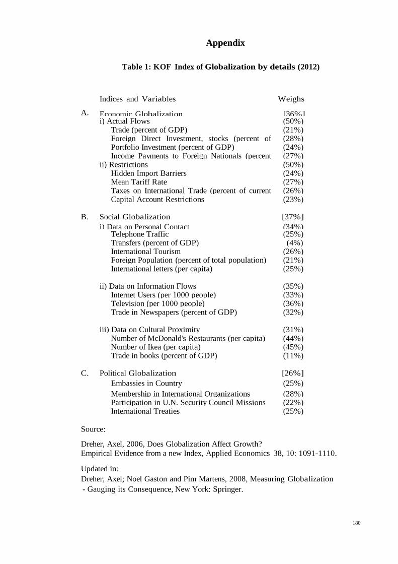
180
10 Appendix
Table 1: KOF Index of Globalization by details (2012)
A.
Indices and Variables
Economic Globalization
Weighs
[36%] i) Actual Flows (50%) Trade (percent of GDP) (21%) Foreign Direct Investment, stocks (percent of
GDP)
(28%) Portfolio Investment (percent of GDP) (24%) Income Payments to Foreign Nationals (percent
of GDP)
(27%) ii) Restrictions (50%) Hidden Import Barriers (24%) Mean Tariff Rate (27%) Taxes on International Trade (percent of current
revenue)
(26%) Capital Account Restrictions (23%)
B.
Social Globalization
i) Data on Personal Contact
[37%]
(34%) Telephone Traffic (25%) Transfers (percent of GDP) (4%) International Tourism (26%) Foreign Population (percent of total population) (21%) International letters (per capita) (25%)
ii) Data on Information Flows
(35%)
Internet Users (per 1000 people) (33%) Television (per 1000 people) (36%) Trade in Newspapers (percent of GDP) (32%)
iii) Data on Cultural Proximity
(31%)
Number of McDonald's Restaurants (per capita) (44%) Number of Ikea (per capita) (45%) Trade in books (percent of GDP) (11%)
C.
Political Globalization
Embassies in Country
[26%]
(25%)
Membership in International Organizations (28%) Participation in U.N. Security Council Missions (22%) International Treaties (25%)
Source:
Dreher, Axel, 2006, Does Globalization Affect Growth?
Empirical Evidence from a new Index, Applied Economics 38, 10: 1091-1110.
Updated in:
Dreher, Axel; Noel Gaston and Pim Martens, 2008, Measuring Globalization
- Gauging its Consequence, New York: Springer.
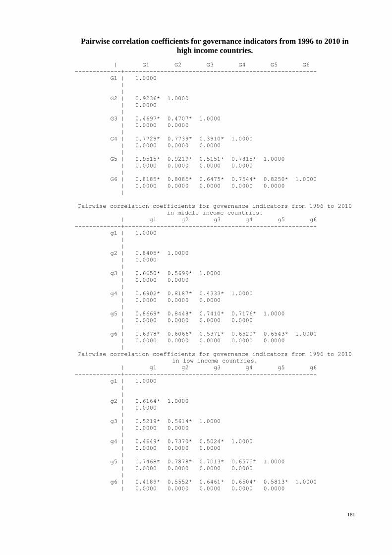
181
Pairwise correlation coefficients for governance indicators from 1996 to 2010 in
high income countries.
| G1 G2 G3 G4 G5 G6
-------------+------------------------------------------------------
G1 | 1.0000
|
|
G2 | 0.9236* 1.0000
| 0.0000
|
G3 | 0.4697* 0.4707* 1.0000
| 0.0000 0.0000
|
G4 | 0.7729* 0.7739* 0.3910* 1.0000
| 0.0000 0.0000 0.0000
|
G5 | 0.9515* 0.9219* 0.5151* 0.7815* 1.0000
| 0.0000 0.0000 0.0000 0.0000
|
G6 | 0.8185* 0.8085* 0.6475* 0.7544* 0.8250* 1.0000
| 0.0000 0.0000 0.0000 0.0000 0.0000
|
Pairwise correlation coefficients for governance indicators from 1996 to 2010
in middle income countries.
| g1 g2 g3 g4 g5 g6
-------------+------------------------------------------------------
g1 | 1.0000
|
|
g2 | 0.8405* 1.0000
| 0.0000
|
g3 | 0.6650* 0.5699* 1.0000
| 0.0000 0.0000
|
g4 | 0.6902* 0.8187* 0.4333* 1.0000
| 0.0000 0.0000 0.0000
|
g5 | 0.8669* 0.8448* 0.7410* 0.7176* 1.0000
| 0.0000 0.0000 0.0000 0.0000
|
g6 | 0.6378* 0.6066* 0.5371* 0.6520* 0.6543* 1.0000
| 0.0000 0.0000 0.0000 0.0000 0.0000
|
Pairwise correlation coefficients for governance indicators from 1996 to 2010
in low income countries.
| g1 g2 g3 g4 g5 g6
-------------+------------------------------------------------------
g1 | 1.0000
|
|
g2 | 0.6164* 1.0000
| 0.0000
|
g3 | 0.5219* 0.5614* 1.0000
| 0.0000 0.0000
|
g4 | 0.4649* 0.7370* 0.5024* 1.0000
| 0.0000 0.0000 0.0000
|
g5 | 0.7468* 0.7878* 0.7013* 0.6575* 1.0000
| 0.0000 0.0000 0.0000 0.0000
|
g6 | 0.4189* 0.5552* 0.6461* 0.6504* 0.5813* 1.0000
| 0.0000 0.0000 0.0000 0.0000 0.0000

182
Pairwise correlation coefficients for Globalization indicators from 1996 to 2010 in
high income countries.
| fdi kof
-------------+------------------
fdi | 1.0000
kof | 0.0293 1.0000

183
World Governance Indicators (WGI) Aggregation Methodology:
Each of six aggregate WGI measures is constructed by averaging together data
from the underlying sources that correspond to the concept of governance being
measured. This is done in the three steps described below.
STEP 1: Assigning data from individual sources to the six aggregate
indicators. Individual questions from the underlying data sources are assigned to each
of the six aggregate indicators. For example, a firm survey question on the regulatory
environment would be assigned to Regulatory Quality, or a measure of press freedom
would be assigned to Voice and Accountability. A full description of the individual
variables used in the WGI and how they are assigned to the six aggregate indicators, can
be found by clicking on the names of the six aggregate indicators listed above. Note that
not all of the data sources cover all countries, and so the aggregate governance scores
are based on different sets of underlying data for different countries.
STEP 2: Preliminary rescaling of the individual source data to run from 0 to
1. The questions from the individual data sources are first rescaled to range from 0 to 1,
with higher values corresponding to better outcomes. If, for example, a survey question
asks for responses on a scale from a minimum of 1 to a maximum of 4, we rescale a
score of 2 as (2-min)/(max-min)=(2-1)/3=0.33. When an individual data source
provides more than one question relating to a particular dimension of governance, we
average together the rescaled scores. The 0-1 rescaled data from the individual sources
are available interactively through the WGI website here, in the country data sheets, and
in the data files for each individual source. Although nominally in the same 0-1 units,
this rescaled data is not necessarily comparable across sources. For example, one data
source might use a 0-10 scale but in practice most scores are clustered between 6 and
10, while another data source might also use a 0-10 scale but have responses spread out

184
over the entire range. While the max-min rescaling above does not correct for this
source of non-comparability, the procedure used to construct the aggregate indicators
does (see below).
STEP 3: Using an Unobserved Components Model (UCM) to construct a
weighted average of the individual indicators for each source. A statistical tool known
as an Unobserved Components Model (UCM) is used to make the 0-1 rescaled data
comparable across sources, and then to construct a weighted average of the data from
each source for each country. The UCM assumes that the observed data from each
source are a linear function of the unobserved level of governance, plus an error
term. This linear function is different for different data sources, and so corrects for the
remaining non-comparability of units of the rescaled data noted above.
The resulting estimates of governance are a weighted average of the data from each
source, with weights reflecting the pattern of correlation among data sources. Click
here for the weights applied to the component indicators.
The UCM assigns greater weight to data sources that tend to be more strongly
correlated with each other. While this weighting improves the statistical precision of
the aggregate indicators, it typically does not affect very much the ranking of countries
on the aggregate indicators. The composite measures of governance generated by the
UCM are in units of a standard normal distribution, with mean zero, standard deviation
of one, and running from approximately -2.5 to 2.5, with higher values corresponding to
better governance. We also report the data in percentile rank term, ranging from 0
(lowest rank) to 100 (highest rank).