Embed Size (px)
Citation preview

CONVECTIVE HEAT TRANSFER AND EXPERIMENTAL
ICING AERODYNAMICS OF WIND TURBINE BLADES
By
Xin Wang
B.A. Sc. (Engineering) North China Electric Power University, 1989
M.A. Sc. (Engineering) Xi’an Jiaotong University, 1996
A THESIS SUBMITED IN PARTIAL FULFILMENT OF
THE REQUIREMENTS FOR THE DEGREE OF
DOCTOR OF PHILOSOPHY
In
THE FACULTY OF GRADUATE STUDIES
DEPARTMENT OF MECHANICAL AND
MANUFACTURING ENGINEERING
UNIVERSITY OF MANITOBA
August, 2008
Copyright © Xin Wang 2008
Convective heat transfer and experimental icing aerodynamics
I
Abstract
The total worldwide base of installed wind energy peak capacity reached 94 GW by the end of
2007, including 1846 MW in Canada. Wind turbine systems are being installed throughout
Canada and often in mountains and cold weather regions, due to their high wind energy potential.
Harsh cold weather climates, involving turbulence, gusts, icing and lightning strikes in these
regions, affect wind turbine performance. Ice accretion and irregular shedding during turbine
operation lead to load imbalances, often causing the turbine to shut off. They create excessive
turbine vibration and may change the natural frequency of blades as well as promote higher
fatigue loads and increase the bending moment of blades. Icing also affects the tower structure by
increasing stresses, due to increased loads from ice accretion. This can lead to structural failures,
especially when coupled to strong wind loads. Icing also affects the reliability of anemometers,
thereby leading to inaccurate wind speed measurements and resulting in resource estimation
errors. Icing issues can directly impact personnel safety, due to falling and projected ice. It is
therefore important to expand research on wind turbines operating in cold climate areas. This
study presents an experimental investigation including three important fundamental aspects: 1)
heat transfer characteristics of the airfoil with and without liquid water content (LWC) at varying
angles of attack; 2) energy losses of wind energy while a wind turbine is operating under icing
conditions; and 3) aerodynamic characteristics of an airfoil during a simulated icing event. A
turbine scale model with curved 3-D blades and a DC generator is tested in a large refrigerated
wind tunnel, where ice formation is simulated by spraying water droplets. A NACA 63421 airfoil
is used to study the characteristics of aerodynamics and convective heat transfer. The current,
voltage, rotation of the DC generator and temperature distribution along the airfoil, which are
used to calculate heat transfer coefficients, are measured using a Data Acquisition (DAQ) system
and recorded with LabVIEW software. The drag, lift and moment of the airfoil are measured by a
force balance system to obtain the aerodynamics of an iced airfoil. This research also quantifies
the power loss under various icing conditions. The data obtained can be used to valid numerical
data method to predict heat transfer characteristics while wind turbine blades worked in cold
climate regions.

Convective heat transfer and experimental icing aerodynamics
II
Table of contents
Abstract ............................................................................................................................................I
Table of contents ............................................................................................................................ II
Table of figures .............................................................................................................................. V
Tables ............................................................................................................................................. X
Nomenclature ................................................................................................................................XI
Acknowledgements .................................................................................................................... XIV
Chapter 1 ......................................................................................................................................... 1
1.1 Background ...........................................................................................................................1
1.1.1. Developing wind energy in the world ...................................................................1
1.1.2. Effects of icing on wind energy ............................................................................4
1.1.3. Ice types in cold climates ......................................................................................5
1.2 Objectives..............................................................................................................................9
1.3 Methodology .......................................................................................................................10
Chapter 2 ....................................................................................................................................... 16
2.1 Weather conditions for wind energy applications...............................................................17
2.2 The technology development of wind energy .....................................................................19
2.3 Aerodynamics of wind turbine blades.................................................................................21
2.3.1 Airfoils applied in wind turbines.........................................................................21
2.3.2 The range of Reynolds number in the aerodynamics study ................................22
2.4 Design and application of wind turbine blades ...................................................................23
2.5 Aerodynamics of the airfoils ...............................................................................................25
2.5.1 Simulation of aerodynamics and theoretical study of airfoils.............................25
2.5.2 Experimental study of aeroelastics of airfoils .....................................................26
2.6 Aerodynamic study of wind turbines ..................................................................................29
2.6.1 Investigation of wind turbine blades ...................................................................29
2.6.2 Flow characteristics study of wind turbines........................................................30
2.7 Icing of wind turbines and blades........................................................................................31

Convective heat transfer and experimental icing aerodynamics
III
2.7.1 Operation of wind turbines under cold climates .................................................31
2.7.2 Icing of airfoils on aircraft ..................................................................................33
2.7.3 Investigation of wind turbine blades with ice ....................................................36
2.8 Research on anti-icing and de-icing for wind turbine blades..............................................38
2.8.1 Simulation study..................................................................................................38
2.8.2 Application of anti-icing or de-icing methods ....................................................39
2.9 Convective heat transfer ......................................................................................................41
2.9.1 Correlation of heat transfer without droplets ......................................................41
2.9.2 Analytical and numerical convection heat transfer .............................................42
2.9.3 Experimental procedures of convection heat transfer .........................................43
2.9.4 Characteristics of water droplet spray.................................................................45
2.9.5 Multi-phase convective heat transfer ..................................................................47
2.10 Operation of wind turbines................................................................................................48
2.11 Summary ...........................................................................................................................52
Chapter 3 ....................................................................................................................................... 55
3.1 Icing wind tunnel and instrumentation................................................................................56
3.1.1 Overall capability and sub-system components ..................................................56
3.1.2 Water spray system .............................................................................................59
3.2 HAWT with 3-D twisted blade operation under icing conditions.......................................61
3.2.1 Fabrication of small wind turbine model ............................................................61
3.2.2 Measurement of rotation, current and voltage ...................................................65
3.3 Aerodynamic force characterization during icing ...............................................................69
3.3.1 Force balance measurements...............................................................................69
3.3.2 Aerodynamics measurements..............................................................................72
3.4 Convective heat transfer characterization of wind blades...................................................75
3.4.1 Setup of heat transfer for an airfoil .....................................................................75
3.4.2 Temperature measurements.................................................................................78
3.4.3 Test procedures and analysis...............................................................................80
Chapter 4 ....................................................................................................................................... 82
4.1 Characteristics of the 3-blade wind turbine model..............................................................82
4.2 Ice thickness over the wind turbine blades..........................................................................86

Convective heat transfer and experimental icing aerodynamics
IV
4.3 Glaze ice over wind turbine.................................................................................................87
4.4 Power losses with rime iced blades.....................................................................................91
4.5 Summary .............................................................................................................................96
Chapter 5 ....................................................................................................................................... 98
5.1 Cylinder measurements .......................................................................................................99
5.2 Ice shapes on an airfoil ......................................................................................................103
5.3 Aerodynamics of the iced airfoil .......................................................................................111
5.4 Discussion of iced wind turbine results.............................................................................117
Chapter 6 ..................................................................................................................................... 120
6.1 Heat transfer characterization at 0 AOA ...........................................................................121
6.1.2 Sensitivity study for correlation coefficients ....................................................125
6.1.3 Comparison with past methods .........................................................................128
6.2 Nusselt number at varying AOA.......................................................................................133
6.3 Heat transfer characterization with water droplets at 0 AOA ...........................................141
6.4 Modified hilpert correlation with LWC at varying AOA..................................................148
6.5 Summary ...........................................................................................................................159
Chapter 7 ..................................................................................................................................... 161
7.1 Conclusions .......................................................................................................................161
7.2 Recommendations for future research...............................................................................164
References ................................................................................................................................... 166
Appendix A – Lists of published papers ..................................................................................... 187
Appendix B – Measurement uncertainties .................................................................................. 189
Appendix C – Operation manual for force balance (A) .............................................................. 192
Appendix D – Operation manual for force balance (B) .............................................................. 195

Convective heat transfer and experimental icing aerodynamics
V
Table of figures
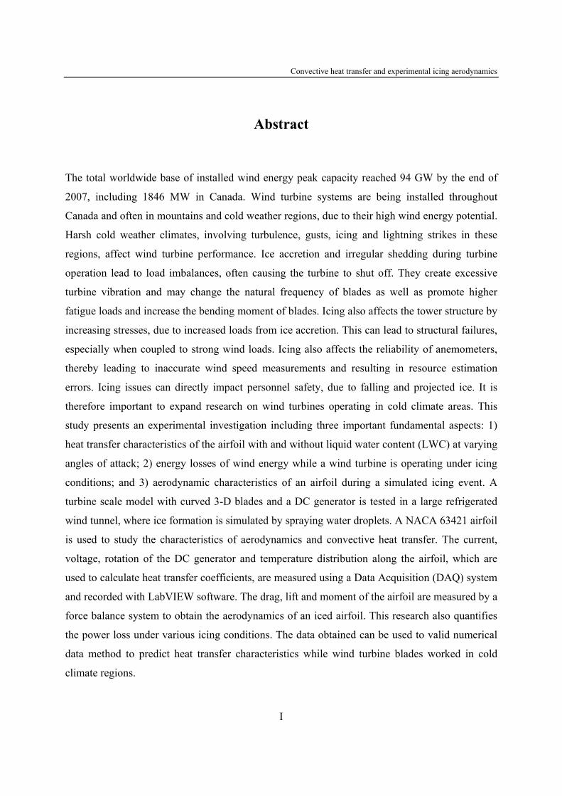
Figure 1.1: Growth rate of annual and cumulative installed capacities of world wind power
(1999-2006) [2] ...........................................................................................................................2
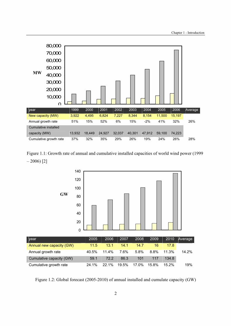
Figure 1.2: Global forecast (2005-2010) of annual installed and cumulate capacity (GW) .......2
Figure 1.3: Distribution of icing and low temperature related consequences in Finland 1996-
2002 [5]. ......................................................................................................................................5
Figure 1.4: Glaze ice in icing tunnel: a) rotating propellers and b) a wind turbine blade model 6
Figure 1.5: Simulated icing event showing rime ice: a) airfoil (icing phase) and b) cylinder
(post icing)...................................................................................................................................8
Figure 1.6: Icing event showing the pre-icing, icing and post icing regions ............................10
Figure 2.1: Wind turbines operating in cold or icing climates ..................................................17
Figure 2.2: Distribution of high wind speed regions in Manitoba [11].....................................18
Figure 2.3: Severe Icing Map – From Manitoba Hydro............................................................19
Figure 2.4: Growth in size and capacity of wind turbine design...............................................20
Figure 3.1: Top view of wind tunnel.........................................................................................57
Figure 3.2: Side View of spray flow / ice tunnel.......................................................................57
Figure 3.3: Nozzle distribution with heaters and thermocouples inside spray bar....................59
Figure 3.4: Spray bar in the icing wind tunnel ..........................................................................60
Figure 3.5: Water flowmeter and air pressure controller. .......................................................61
Figure 3.6: Digitized blade: a) smooth blade and b) blade before smoothing ..........................62
Figure 3.7: a) a blade model at 0 pitch angle and b) blades with adaptors. ..............................63
Figure 3.8: a) hub and b) hub center .........................................................................................64

Convective heat transfer and experimental icing aerodynamics
VI
Figure 3.9: Wind turbine model with DC generator in the wind tunnel ...................................65
Figure 3.10: Circuit diagram of current and voltage transducer with DC generator.................67
Figure 3.11: PC-based data acquisition system.........................................................................68
Figure 3.12: Structure of the side wall force balance................................................................69
Figure 3.13: Side view of one balance wall with a shaft coupler..............................................69
Figure 3.14: Data acquisition system: HBM MGC Plus and a Laptop .....................................70
Figure 3.15: Acquisition of data from FMS force measurement system ..................................71
Figure 3.16: Tunnel setup for icing of airfoil measurements ....................................................71
Figure 3.17: NACA 63421 airfoil with thermocouple locations (note: dimensions in mm).....77
Figure 3.18: Test airfoil with a heater and thermocouples........................................................77
Figure 3.19: Block panel of LabVIEW: temperature, voltage and frequency measurement ....78
Figure 3.20: The front panel of Temperature, rotation and voltage measuring with LabView 8.
...................................................................................................................................................79
Figure 4.1: Power output at different pitch angels ....................................................................83
Figure 4.2: Rotation at different pitch angles............................................................................84
Figure 4.3: Power output at different temperatures...................................................................85
Figure 4.4: Rotation variation at different temperatures ...........................................................85
Figure 4.5: Glaze ice over a wind turbine .................................................................................88
Figure 4.6: Icing of blades at -2°C for 2, 5 and 10 minutes ......................................................88
Figure 4.7: Comparison power losses for different ice thicknesses ..........................................89
Figure 4.8: Comparison rotation for different ice thicknesses ..................................................90
Figure 4.9: Power output and 4.2 mm ice thickness .................................................................91
Figure 4.10: Rime ice on the wind turbine blade ......................................................................92

Convective heat transfer and experimental icing aerodynamics
VII
Figure 4.11: Power losses at extreme icing conditions .............................................................94
Figure 4.12: Rotation of the turbine working on extreme weather condition for different ice
thicknesses.................................................................................................................................94
Figure 4.13: Wind energy losses under -20°C: a) power output; b) rotation ............................95
Figure 5.1: Shorter cylinder installed in the wind tunnel with force balance and shaft
protectors ...................................................................................................................................99
Figure 5.2: CD of different diameter cylinders as a function of Reynolds numbers................100
Figure 5.3: Comparison with short and long cylinders for CL and CD ....................................101
Figure 5.4: Rime iced cylinder at -9, 0.8 g/m3 and 10 m/s at 30 minutes spraying ............102
Figure 5.5: Two airfoils in tendam installed in the icing wind tunnel ....................................103
Figure 5.6: Left side of the force balance with a camera ........................................................104
Figure 5.7: Photograph of an iced airfoil at -9, 10 m/s and 0.8 g/m3 ..................................105
Figure 5.8: Ice shape over the airfoil at -9, 10 m/s and 0.8 g/m3 during 45 minutes ..........106
Figure 5.9: Aerodynamics of iced airfoils with glaze ice at various AOA .............................113
Figure 5.10: Aerodynamics of iced airfoils with rime ice at various AOA and spraying
duration: a) AOA = 0°& 6°; b) AOA = 3°& 9°with 0.8 g/m3 LWC at 10 m/s wind speed ....115
Figure 6.1: Average Nusselt number at varying Reynolds and Prandtl numbers ...................122
Figure 6.2: Normalized Nusselt function correlation..............................................................124
Figure 6.3: Local Nusselt number at varying chord positions (x/c) ........................................124
Figure 6.4: Average Nusselt number at varying a) c and b) m (Rec ≤ 5 ×10⁵) .......................126
Figure 6.5: Average Nusselt number at varying a) c and b) m (Rec > 5 ×10⁵) .......................127
Figure 6.6: Local Nusselt number for cylinder and airfoil cases ............................................129
Figure 6.7: Comparison between NACA airfoil, flat plate and circular cylinder results........132
Convective heat transfer and experimental icing aerodynamics
VIII
Figure 6.8: Local Nusselt number distribution along dimensionless chord: a) low Re, and b)
high Re.....................................................................................................................................135
Figure 6.9: Measured data and Nusselt number correlation at various AOA (high Rec) ........136
Figure 6.10: Measured data and Nu correlation at 10° AOA (low Rec)..................................137
Figure 6.11: Measured data and Nu correlation at varying AOA from 5° to 25° (low Rec)...137
Figure 6.12: Comparison of measured data dotted at 10° and Nu correlations at 0° & 10° AOA
.................................................................................................................................................140
Figure 6.13: Comparison of experimental data with LWC and Nusselt function correlations
without LWC: a) high Re and b) low Re.................................................................................142
Figure 6.14: Local Nusselt number at varying chord positions (x/c) ......................................144
Figure 6.15: Predicted and measured Nu a) without and b) with droplets for Rec (1+W) > 6 ×
105............................................................................................................................................145
Figure 6.16: Predicted and measured Nu a) without and b) with droplets for Rec (1+W) ≤ 6
×105 ........................................................................................................................................146
Figure 6.17: Measured data and predicted Nu correlation at a) high Rec and b) low Rec at 15°
AOA ........................................................................................................................................150
Figure 6.18: Comparison of measured data with LWC and Nu correlations without LWC at
15° AOA, as well as the predicted Nu correlation with LWC at 0° AOA ..............................152
Figure 6. 19: Nusselt number at a) low and b) high Reynolds numbers with LWC at varying
AOA ........................................................................................................................................154
Figure 6.20: Predicted and measured Nu with droplets for Rec (1+W) > 6×10⁵ at 15° AOA 157
Figure 6.21: Measured date and predicted Nu with droplets at varying angles of attack for high
Rec (1+W)................................................................................................................................158

Convective heat transfer and experimental icing aerodynamics
IX
Figure 6.22: Predicted and measured Nu with droplets for Rec (1+W) ≤ 6×10⁵ at 15° AOA 158
Figure 6.23: Predicted and measured Nu with droplets for Rec (1+W) ≤ 6×10⁵ at varying AOA
.................................................................................................................................................159
Convective heat transfer and experimental icing aerodynamics
X
Tables
Table 1.1: Canada’s wind energy Tracker by July 2007..................................................................3
Table 1.2:‘Ice Alarm’ indication from Manitoba Hydro’s System Control Centre 1999- 2006....14
Table 3.1: Test content in the investigation ...................................................................................55
Table 3.2: Standard deviation of calibration results (6 × 39 Non-Iterative) ..................................70
Table 3.3: Past literature for airfoils and range of Reynolds numbers...........................................73
Table 3.4: Heat transfer and simulated icing conditions................................................................75
Table 4.1: Wind turbine operating conditions................................................................................82
Table 4.2: Glaze ice thicknesses over the wind turbine blades (-3°C) (mm).................................86
Table 4.3: Rime ice thicknesses over the wind turbine blades (-10°C) (mm) ...............................87
Table 4.4: Ice thicknesses at -20°C and -30°C on the wind turbine blades (mm) .........................87
Table 5.1: Icing conditions for aerodynamics studies....................................................................98
Table 5.2: Photos of glaze ice at various AOAs and spraying times at -5 and 10 m/s ...........107
Table 5.3: Glaze ice shapes at various AOA and spraying duration at -5 and 10 m/s .............108
Table 5.4: Pictures of rime ice at various AOA and spraying duration at -9 and 10 m/s ........109
Table 5.5: Rime ice shapes at various AOA and spraying duration at -9 and 10 m/s..............110
Table 5.6: Data of ∆CL, ∆CD and ∆Cm at -5ºC (0.8 g/m3 LWC and 10 m/s wind speed)............112
Table 5.7: Rime ice aerodynamics of the iced airfoil at tunnel temperature -9ºC .......................113
Table 6.1: Experimental conditions during convective heat transfer...........................................121
Table 6.2: The range of Prandtl numbers in the experiments ......................................................121

Convective heat transfer and experimental icing aerodynamics
XI
Nomenclature
c chord of airfoil (m)
C1, C2 chord coefficient
CD drag coefficient
CL lift coefficient
cm moment center (m)
Cm moment coefficient
D diameter of wind turbine m,
D1, D2, D3, D4 arc angle coefficients
FX force in the X axis direction (N)
FZ measured force in the Z axis direction (N)
FD drag force (N)
FL lift force (N)
hi local convective heat transfer coefficient (W/m2K)
h average heat transfer coefficient (W/m2K)
i local measurement point in the 2-D airfoil
k thermal conductivity (W/mK)
k height of ice (m)
K dimensionless shear parameter
L span of airfoil (m)
M1, M2, M3 ice thickness at the middle of wind turbine No. 1, 2, 3 blades (mm)
M moment (Nm)

Convective heat transfer and experimental icing aerodynamics
XII
Nux local Nusselt number
Nu average Nusselt number
P power output of the 3-blade wind turbine (W)
Pr Prandtl number
P*, *maxP maximum power output of the 3-blade wind turbine at 20°C temperature (W)
qcon convective heat flux (W)
qcd conductive heat flux (W)
R2 curve regression coefficient
Rec Reynolds number (based on a chord reference length)
ReD Reynolds number (based on a diameter of the 3-blade wind turbine)
Rem Multiphase Reynolds number
ReL Reynolds number (based on a length of a flat plate)
Rex Reynolds number (based on a local position of a flat plate)
R1, R2, R3 ice thickness at the root of wind turbine No.1, 2, 3 blades (mm)
s circumference of the 2-D airfoil model
s position of ice on an airfoil surface (m)
si distance between two measurement points in the 2-D airfoil
T∞ freestream temperature (oC)
Tin inner surface temperature of airfoil (oC)
To outer surface temperature of airfoil (oC)
W non-dimensional liquid water content
u∞ velocity of free stream m/s
AOA angle of attack (°)

Convective heat transfer and experimental icing aerodynamics
XIII
ANN artificial neural networks
CFD computational fluid dynamics
CHF critical heat flux (W/m2)
HTC heat transfer coefficient
LCE local collision efficiency
LWC liquid water content (g/m3)
MVD mean volume diameter (µm)
NACA National Advisory Committee for Aeronautics
NASA National Aeronautics and Space Administration
NAG numerical algorithms group
NREL National Renewable Energy Laboratory
PDA laser phase-doppler anemometry
PIV particle image velocimetry
RPM rotation of the 3-blade wind turbine (Hz)
RPM* maximum rotation of the 3-blade wind turbine at 20°C temperature
TSR tip speed ratio
Greek Symbol
µ dynamic viscosity of air (kg/ms)
ρ density of air (kg/m3)
δ average thickness of the airfoil (mm)
δ ice thickness over the blades (mm)
α angle of attack (°)

Convective heat transfer and experimental icing aerodynamics
XIV
Acknowledgements
My first and most earnest acknowledgment must go to my advisors: Dr. E.L. Bibeau and Dr. G.F.
Naterer. Dr. Naterer and Dr. Bibeau have been instrumental in ensuring my academic,
professional, financial and moral well being ever since I started to work with them. In every
sense, none of this work would have been possible without them. They gave excellent advice to
me about this research project and written thesis. Many thanks also to committee members Dr. J.
Hanesiak and Dr. S. J. Ormiston. The financial support of the Natural Sciences and Research
Council of Canada (NSERC), Manitoba Hydro NSERC Chair in Alternative Energy, Tier 1
Canada Research Chair in Advanced Energy Systems and the Canada Foundation for Innovation
(CFI) are gratefully appreciated.
Far too many people to mention individually have assisted in so many ways during my research
work at UM. They all have my sincere gratitude. In particular, I would like to thank Dr. Qingjin
Peng for providing assistance in reverse engineering for a blade model, Mr. Qing Sun for help in
experimental and research assistance, and technical help provided by Mr. Bruce Ellis and Mr.
Paul Krueger.
I also wish to thank my family and friends for their encouragement and support. My final, and
most heartfelt acknowledgment must go to my wife Xiaofei Pang who has worked diligently and
successfully. Her support, encouragement, and companionship have converted my journey
through graduate school into a pleasure.

1
Chapter 1
Introduction
1.1 Background
1.1.1. Developing wind energy in the world
Climate change could become one of the most important problems this century. Efforts must be
made by all countries to reduce industrialized GHG emissions by at least 30% by 2020 according
to calculations by the European Wind Energy Association [1] to keep the global mean
temperature rise below 2°C. Many countries, including Canada, are developing wind power
generation capacity to meet the rising demand for energy using renewable power. Figure 1.1
shows the annual growth in the world wind power market from 1999 to 2006 [2]. It is predicted
that the total installed capacity of wind energy will increase to 135 GW worldwide and reach an
average growth rate of 19.1% by 2010 as compared to the average 24.3% growth rate from 2002
to 2006 [2].
Figure 1.2 exhibits the planned growth rate from 2005 to 2010 [3] in the world. Comparing the
capacity of the planned and installed capacities in 2005 and 2006, it can be found that global
wind energy has developed faster than anticipated and this will be a booming industry for many
years.
Chapter 1 - Introduction
2
010,00020,00030,00040,00050,00060,00070,00080,000
year 1999 2000 2001 2002 2003 2004 2005 2006 Average
New capacity (MW) 3,922 4,495 6,824 7,227 8,344 8,154 11,500 15,197
Annual growth rate 51% 15% 52% 6% 15% -2% 41% 32% 26%
Cumulative installed
capacity (MW) 13,932 18,449 24,927 32,037 40,301 47,912 59,100 74,223
Cumulative growth rate 37% 32% 35% 29% 26% 19% 24% 26% 28%
Figure 1.1: Growth rate of annual and cumulative installed capacities of world wind power (1999
– 2006) [2]
0
20
40
60
80
100
120
140
year 2005 2006 2007 2008 2009 2010 Average
Annual new capacity (GW) 11.5 13.1 14.1 14.7 16 17.8
Annual growth rate 40.5% 11.4% 7.6% 5.8% 8.8% 11.3% 14.2%
Cumulative capacity (GW) 59.1 72.2 86.3 101 117 134.8
Cumulative growth rate 24.1% 22.1% 19.5% 17.0% 15.8% 15.2% 19%
Figure 1.2: Global forecast (2005-2010) of annual installed and cumulate capacity (GW)
MW
GW

Chapter 1 - Introduction
3
The previous figures provide an indication of projected wind energy capacity and a global
outlook. Canada has a strong potential for wind energy development. Wind turbine systems are
being installed throughout Canada and often in mountains and cold weather regions. The
Canadian Federal Government expanded its Wind Power Incentive Program in the 2005 budget
to support the development of an additional 4,000 MW of wind energy by 2010 [3]. Furthermore,
from the GWEA 2007 annual report, Canada’s provincial governments have now set targets and
objectives for wind energy development that will have a minium total of 12,000 MW by 2016 [2].
This includes wind energy in cold weather areas, such as Manitoba, which plans to develop 1,000
MW wind energy capacity from 2009 to 2014, according to the Manitoba Provincial Government.
This can be compared with Quebec, which forecasts about 3,500 MW of wind energy by 2012 to
offset the shortfall in power supply. Table 1.1 shows Canada’s wind tracker by July 2007 [4]. It
can be found that more and more wind energy facilities will be installed in cold and icing climate
areas in Canada.
Table 1.1: Canada’s wind energy Tracker by July 2007
Province Installed Proposed* BC 0 325.2 MW Alberta 442.6 MW 80.0 MW Saskatchewan 171.2 MW 24.8 MW Manitoba 103.9 MW 0.0 MW Ontario 415.3 MW 1014.8 MW Quebec 321.8 MW 1095.0 MW Newfoundland 390.0 KW 51.0 MW PEI 72.4 MW 79.2 MW Nova Scotia 59.3 MW 1.2 MW New Brunswick 0.0 96.0 MW Yukon 810.0 kW 0.0 NWT 0.0 0.0 Nunavut 0.0 0.0 Total 1587.6 MW 2767.1 MW *Under construction or awarded a PPA

Chapter 1 - Introduction
4
1.1.2. Effects of icing on wind energy
Climatic conditions with turbulence, gusts, icing and lightning strikes in cold regions will affect
wind turbine performance and cause idling of wind farms on windy days. In particular, ice
accretion and irregular shedding during turbine operation cause large load imbalances as well as
excessive turbine vibration. They can change the natural frequency of blades, promote higher
fatigue loads, and increase the bending moment of blades. Icing affects the tower structure by
increasing stresses due to increased loads from ice accretion. This can lead to structural failures,
especially when coupled with strong wind loads. Icing also affects the reliability of anemometers
and sensors, thereby leading to inaccurate wind speed measurements, thereby resulting in
resource estimation errors. These icing issues can directly impact personnel safety due to falling
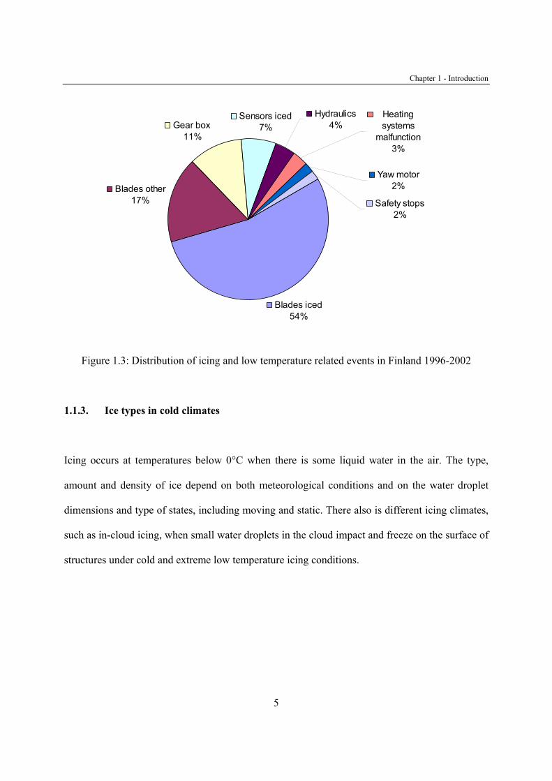
ice. Figure 1.3 shows that the distribution of icing and low temperature related consequences in
Finland from 1996 – 2002 included a total of 12,629 hours [5]. Ronsten [6] also reported a
stoppage of over 7 weeks of a wind turbine due to icing, during the best operating period in
southern Sweden. These facts show icing and cold conditions will in some cases significantly
affect the operation of the wind turbines installed, or that will be serviced in the cold climate such
as North America and North Europe. Also, a total 71% of consequences, including 54% iced
wind turbine blades and other blade problems indicate that the wind turbine blades are the most
important and frequent malfunctioning parts when a wind turbine is working in icing areas, due
to ice on the blades. This can introduce important geometric changes to their leading edges and
cause rapid variations in lift and drag. More research focused on icing of wind turbine blades is
required to obtain insight of aerodynamics of airfoils and de-ice or anti-ice methods.
Chapter 1 - Introduction
5
Heating systems
malfunction3%
Yaw motor 2%
Hydraulics4%
Sensors iced 7%Gear box
11%
Blades other 17%
Blades iced 54%
Safety stops 2%
Figure 1.3: Distribution of icing and low temperature related events in Finland 1996-2002
1.1.3. Ice types in cold climates
Icing occurs at temperatures below 0°C when there is some liquid water in the air. The type,
amount and density of ice depend on both meteorological conditions and on the water droplet
dimensions and type of states, including moving and static. There also is different icing climates,
such as in-cloud icing, when small water droplets in the cloud impact and freeze on the surface of
structures under cold and extreme low temperature icing conditions.
Chapter 1 - Introduction
6
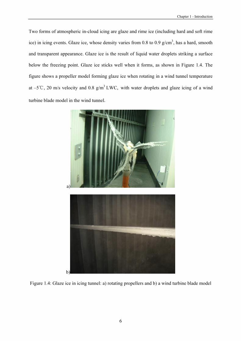
Two forms of atmospheric in-cloud icing are glaze and rime ice (including hard and soft rime
ice) in icing events. Glaze ice, whose density varies from 0.8 to 0.9 g/cm3, has a hard, smooth
and transparent appearance. Glaze ice is the result of liquid water droplets striking a surface
below the freezing point. Glaze ice sticks well when it forms, as shown in Figure 1.4. The
figure shows a propeller model forming glaze ice when rotating in a wind tunnel temperature
at –5, 20 m/s velocity and 0.8 g/m3 LWC, with water droplets and glaze icing of a wind
turbine blade model in the wind tunnel.
a)
b)
Figure 1.4: Glaze ice in icing tunnel: a) rotating propellers and b) a wind turbine blade model

Chapter 1 - Introduction
7
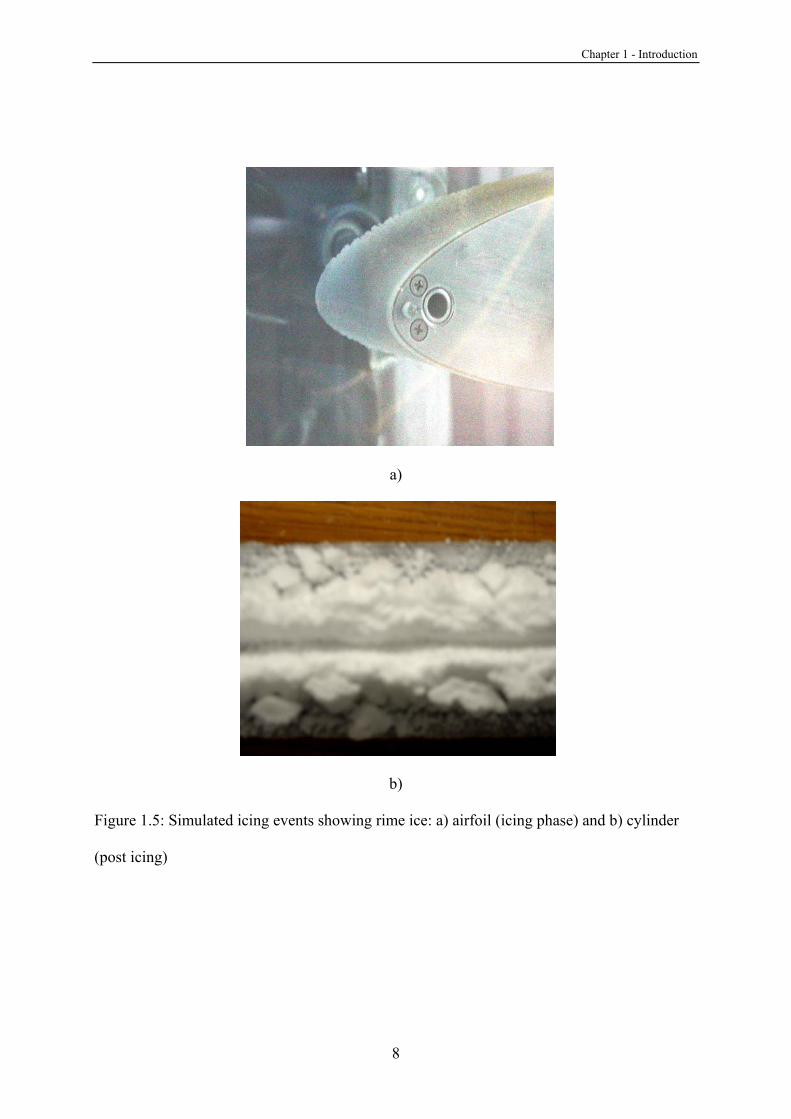
Rime ice has a rough and opaque appearance and forms when the surface temperature is
below the freezing point and it is exposed to supercooled water droplets. Due to the presence
of air bubbles trapped inside, rime ice is opaque and its density ranges from 0.59 to 0.9 g/cm3,
depending on the type of ice. Druez et al. [7] experimentally studied mechanical property
variations of atmospheric ice, including rime ice, with air velocity, liquid water content (LWC)
and temperature and median volume droplet diameter (MVD). The results showed that ice
strengths in compression and adhesion increased when the LWC and MVD increased and the
air temperature decreased during ice accretion. However, the density of ice decreased with
increasing air temperature under rime icing conditions. Figure 1.5 shows rime ice on an
airfoil blade and a cylinder. Unlike glaze ice, rime ice accretes horizontally and forms various
shapes in the upwind direction. Another kind of icing is called precipitation icing, including
wet snow and freezing rain. Freezing rain is anticipated to become more serious due to global
warming.
Many studies have contributed to our present understanding of the aerodynamic effects of
icing of wind turbine blades. Most of the work has focused on simulated ice shapes over
airfoils in wind tunnels, at atmospheric conditions at very high wind velocity, such as iced
wings of an aircraft. It is therefore important to expand research on wind turbines operating in
cold climate areas and focus on developing a more fundamental understanding of these
complex phase change phenomena for wind turbines.
Chapter 1 - Introduction
8
a)
b)
Figure 1.5: Simulated icing events showing rime ice: a) airfoil (icing phase) and b) cylinder
(post icing)

Chapter 1 - Introduction
9
1.2 Objectives
This proposed research will concentrate on three important inter-related aspects of icing of
wind turbine blades to improve our fundamental understanding of icing of wind turbines, with
experiments performed during simulated icing events.
Operational Effects: A 3-D wind turbine model was built and it will be used to measure the
power output at various pitch angles and icing conditions to relate the changes of the
aerodynamic forces to power reduction, when a wind turbine is operating under icing
conditions. Ice accretion and irregular shedding during turbine operation causes large load
imbalances, creating excessive turbine vibration. They can change the natural frequency of
blades, promoting higher fatigue loads and increases in the bending moment of blades. This
thesis will quantify the power loss under various icing conditions, which is an important
aspect to ensure proper operation by wind farm operators. Knowledge gained in determining
the impact of aerodynamic forces and heat transfer characterization will provide new insights
into these operational issues.
Aerodynamic Forces: An important part of the research will be to examine the aerodynamics
of airfoils including the lift, drag and moment coefficient variations during a simulated icing
event, which includes the pre-icing, icing and post icing periods. Special attention will be
given to better understand the droplet capture efficiency of wind turbine blades. This aspect is
important to predict ice accretion rates and provide transient icing data for numerical model
validation. The pressure gradient at the leading edge of the blade affects both the heat transfer
and the aerodynamic forces. Both aspects need to be understood. Determining how they are
related is important to develop ice mitigation strategies.

Chapter 1 - Introduction
10
Water filmForming iceover surface
Super-cooledwater droplets
Iced airfoil
Airfoil withheater
Cold air flow without water droplets.
Airfoil Airfoil
Cold air flow with water droplets.
Figure 1.6: Icing event showing the pre-icing, icing and post icing stages
Heat Transfer: The objective of the proposed research is also to improve our knowledge of
the mechanism of heat transfer, when air flows over a turbine blade under different conditions,
representing some of the following icing stages, shown in Figure 1.6: low temperature
experiment without liquid water content (LWC); room temperature with some LWC; and
icing conditions with super-cooled water droplets. Heat transfer characterization at various
points along the blade is a key requirement to develop effective heat and mass balance models
over the turbine blade and predict power requirements for thermal mitigation strategies and
blade performance changes. Better characterization of the heat transfer may lead, for example,
to lower power requirements with electrical heating of the leading edge during an icing event.
1.3 Methodology
To achieve these research objectives, an icing wind tunnel is used. It includes a) a 3-blade
scaled model to simulate wind turbine rotating blades, b) an image capture (digital camera)
system to determine shapes of the iced airfoil, and c) a force balance to measure transient
aerodynamic forces during an icing event and heat transfer characteristics, while air with

Chapter 1 - Introduction
11
water droplets flow over an airfoil. A water spray system supplies super-cooled water droplets
to simulate icing conditions under lower temperatures for rime and glaze icing conditions.
Thermocouples and a Pitot tube are used to measure the temperature and air velocity,
respectively. The experimental methodology to achieve the research objectives consists of the
following three investigations.
• A rotating 3-blade wind turbine with an electrical generator is used to measure ice
accretion rates during a simulated icing event. These results are used to estimate the
power loss when wind turbines operate under icing conditions. By measuring the
generator current, voltage, temperature, and velocity of wind in the tunnel, it is possible to
study wind turbine behaviors during an icing event. More details about the proposed
experimental work are discussed in Chapter 4. Developing a rotating wind turbine model
is key for fundamental understanding of icing and subsequent mitigation strategies.
• A 2-D airfoil model is used to measure the lift, drag and moment at different angles of
attack during a simulated icing event for rime and glaze conditions. A comparison
between an un-iced airfoil and different iced airfoils is investigated. The measurement of
force and moment is performed with a three-component strain gauge dynamometer force
balance. This includes lift, drag and pitching moment. These experiments characterize the
effects of aerodynamic forces during a simulated icing event, to provide insights into the
complex phase change phenomena. Additional details are also provided in Chapter 5.
• A 2-D NACA 63421 airfoil model is tested in the icing tunnel to determine the convective
heat transfer coefficient. These tests were developed to measure the heat transfer
characteristics for atmospheric air, air with water droplets without phase change, and air
with water droplets and phase change (icing conditions). Each of these tests corresponds
to the pre-icing, icing and post icing regions, as shown in Figure 1.6. The proposed plan

Chapter 1 - Introduction
12
of testing heat transfer characteristics is discussed in Chapter 6, including the
experimental setup of the test model in the wind tunnel, measurement system, results and
analysis. This research work is key to characterize the heat transfer from an airfoil to
simulate icing conditions and provide theoretical background for heating de-icing or anti-
icing.
These three sets of experiments for wind turbine blades during icing conditions provide a
unique set of experimental data to explain heat transfer characteristics of icing of wind turbine
blades. They also provide fundamental insights for better understanding of icing events and
help the development of de-icing or anti-icing wind turbine blade technologies, as well as
more accurate predictive models, and provide model validation data.
It is a challenge to simulate complex icing conditions under wind tunnel conditions, as scaling
laws are not well formulated for sprayed water in wind tunnels. As a result, the predicted
results may have differences compared to actual wind turbine icing conditions. It will be
important to assess these differences. The proposed experiments will give useful data for
better understanding of aerodynamics and heat transfer during wind turbine icing, while
capturing also the important operational issues.
1.4 Significance of this study
This research has both theoretical and practical importance. Currently, there are relatively few
experimental studies which focus on the operation of wind turbines in icing conditions. Some
manufacturers have developed de-icing or anti-icing technology, such as a leading edge

Chapter 1 - Introduction
13
heating foil or microwave de-icing system. However, fundamental knowledge needs to be
improved to address the many technical challenges remaining to be overcome. This should
lead to more cost-effective solutions for wind farms. Most investigations use simulated ice to
measure the lift and drag coefficients of airfoils under icing conditions. Significantly less
attention has been given to the characterization of heat transfer when air flows over the airfoil,
under simulated operating conditions of a wind turbine. The study conducted in this research
will provide useful data regarding heat transfer from blades.
A past article entitled “Prioritizing Wind Energy Research” by EWEA [8] ascertains that the
barriers for developing wind energy include large wind turbine operation in cold climates.
This theme is also reflected in the annual report of IEA [9]. An example here in Canada
recently is the utilization of wind demonstration projects in the Northwest Territories and
Nunavut [10] that show that wind generation in remote Canadian communities has been
adversely affected by cold weather. For example, Sach's Harbour, Northwest Territories,
installed 66 kW wind capacity at a capital cost of $445,000. This operated for 15 months at a
1.5% operating capacity factor resulting in $40.45 per kWhr of power costs (lifetime, capital
cost only). Kugluktuk, Nunavut which installed 160 kW at a capital cost of $650,000,
operated for 39 months at a 5.6% operating capacity factor, resulting in $2.56 per kWh power
costs (lifetime, capital cost only); and Rankin Inlet, Nunavut, installed 66 kW wind capacity
at a capital cost of $355,000, it has been operating since November 2000 at a 8.9% operating
capacity factor, resulting in $1.63 per kWhr of power. These costs are significantly higher
than the approximate $0.09 per kWh normally reported for wind power and reflect the many
operational challenges faced by remote communities, those include cold weather effects.
Chapter 1 - Introduction
14
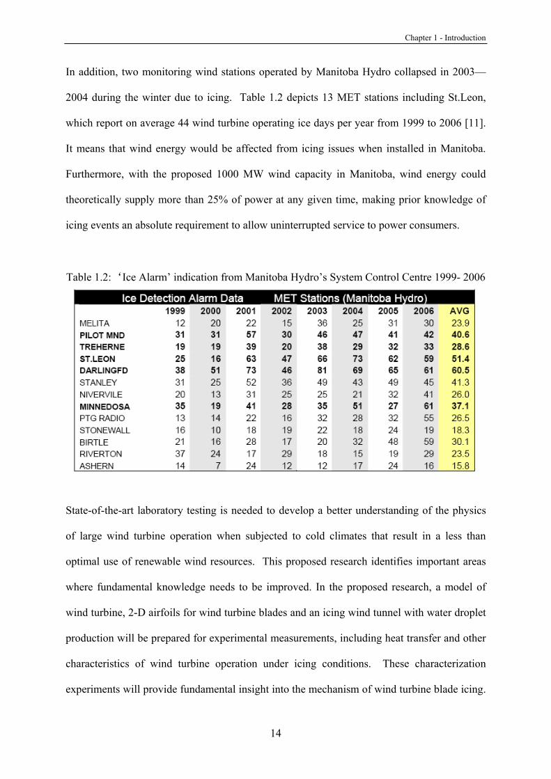
In addition, two monitoring wind stations operated by Manitoba Hydro collapsed in 2003—
2004 during the winter due to icing. Table 1.2 depicts 13 MET stations including St.Leon,
which report on average 44 wind turbine operating ice days per year from 1999 to 2006 [11].
It means that wind energy would be affected from icing issues when installed in Manitoba.
Furthermore, with the proposed 1000 MW wind capacity in Manitoba, wind energy could
theoretically supply more than 25% of power at any given time, making prior knowledge of
icing events an absolute requirement to allow uninterrupted service to power consumers.
Table 1.2:‘Ice Alarm’ indication from Manitoba Hydro’s System Control Centre 1999- 2006
State-of-the-art laboratory testing is needed to develop a better understanding of the physics
of large wind turbine operation when subjected to cold climates that result in a less than
optimal use of renewable wind resources. This proposed research identifies important areas
where fundamental knowledge needs to be improved. In the proposed research, a model of
wind turbine, 2-D airfoils for wind turbine blades and an icing wind tunnel with water droplet
production will be prepared for experimental measurements, including heat transfer and other
characteristics of wind turbine operation under icing conditions. These characterization
experiments will provide fundamental insight into the mechanism of wind turbine blade icing.

Chapter 1 - Introduction
15
Analysis methods will be developed to better understand the physics of wind turbine blade
icing. These tests will also be used to provide validation data for advanced numerical
Computational Fluid Dynamics (CFD) models.

16
Chapter 2
Literature review
As one of the fastest growing renewable energies in the world, wind power has become a
main source of energy for the future. However, wind energy continues to encounter problems
that need to be addressed as the technology is deployed under various climatic conditions.
Past research has shown progress towards better understanding of aerodynamic characteristics
of wind turbines, icing of wind turbine blades, wind sensors, anemometers, nacelles, heating
systems for de-icing or anti-icing of blades and computational simulations. The following
literature review will present current status of icing of wind turbines in Manitoba and some of
those achievements in past research that pertain to the growing issue of icing of wind turbine
blades. The three main objectives of this review focus on operational effects, aerodynamic
forces and characterization of heat transfer.
The literature review includes the following main themes that will be used throughout the
research:
• Weather conditions for wind energy applications;
• The technology development of wind energy;
• Aerodynamics of wind turbine blades;
• Design and application of wind turbine blades;
• Aerodynamics of the airfoils;
• Aerodynamic study of wind turbines;
• Icing of wind turbines and blades;
• Research on anti-icing and de-icing for wind turbine blades;

Chapter 2 - Literature review
17
• Convective heat transfer;
• Operation of wind turbines.
2.1 Weather conditions for wind energy applications
A cold climate is defined as one that experiences either icing events or temperatures lower
than the operational limits of standard wind turbines [12]. Many wind turbines have been
operating in regions that experience cold or icing climates, such as Scandinavia, North
America, Europe, and Asia. Figure 2.1 shows that wind turbines are located in cold or icing
climates [13]. Canada is not included in the map because the survey was pretty old and new
map willl have to include Canada because so many wind turbines installed in cold climates.
However, as mentioned in Table 1.1, significant wind energy capacities have been projected
or planned to be installed in most of the provinces in Canada, including Manitoba where cold
climates with icing conditions occur (yellow circle in Figure 2.1 and red point including
Manitoba, Quebec and Saskatchewan).
Figure 2.1: Wind turbines operating in cold or icing climates (2003) [13]
Chapter 2 - Literature review
18
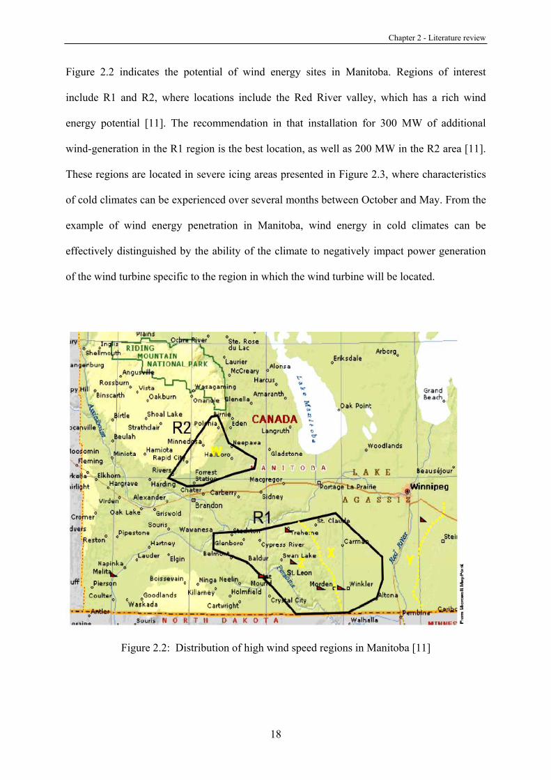
Figure 2.2 indicates the potential of wind energy sites in Manitoba. Regions of interest
include R1 and R2, where locations include the Red River valley, which has a rich wind
energy potential [11]. The recommendation in that installation for 300 MW of additional
wind-generation in the R1 region is the best location, as well as 200 MW in the R2 area [11].
These regions are located in severe icing areas presented in Figure 2.3, where characteristics
of cold climates can be experienced over several months between October and May. From the
example of wind energy penetration in Manitoba, wind energy in cold climates can be
effectively distinguished by the ability of the climate to negatively impact power generation
of the wind turbine specific to the region in which the wind turbine will be located.
Figure 2.2: Distribution of high wind speed regions in Manitoba [11]

Chapter 2 - Literature review
19
Figure 2.3: Severe Icing Map – From Manitoba Hydro [11]
2.2 The technology development of wind energy
There are two kinds of wind turbines that have been developed to transform wind kinetic
energy into mechanical energy and then electric power. These include the horizontal axis
wind turbines (HAWT) and vertical axis wind turbines (VAWT). Presently two kinds of wind
turbines are being installed in the world, including mountains, valleys and offshore. Normally,
the large capacity wind turbines are the horizontal axis type. The capacity of a wind turbine
has been developed from 50 kW to 5000 KW [14] and the diameter of a wind turbine ranges
from 12 m to 126 m (see Figure 2.4 [15]). From 1985 to 2003, the capacity increase of a
single wind turbine has increased tenfold every decade.
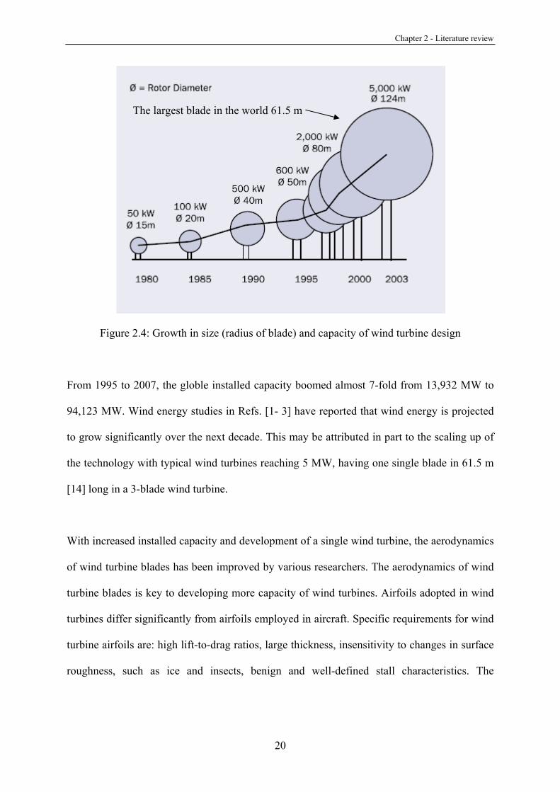
Chapter 2 - Literature review
20
Figure 2.4: Growth in size (radius of blade) and capacity of wind turbine design
From 1995 to 2007, the globle installed capacity boomed almost 7-fold from 13,932 MW to
94,123 MW. Wind energy studies in Refs. [1- 3] have reported that wind energy is projected
to grow significantly over the next decade. This may be attributed in part to the scaling up of
the technology with typical wind turbines reaching 5 MW, having one single blade in 61.5 m
[14] long in a 3-blade wind turbine.
With increased installed capacity and development of a single wind turbine, the aerodynamics
of wind turbine blades has been improved by various researchers. The aerodynamics of wind
turbine blades is key to developing more capacity of wind turbines. Airfoils adopted in wind
turbines differ significantly from airfoils employed in aircraft. Specific requirements for wind
turbine airfoils are: high lift-to-drag ratios, large thickness, insensitivity to changes in surface
roughness, such as ice and insects, benign and well-defined stall characteristics. The
The largest blade in the world 61.5 m
Chapter 2 - Literature review
21
following section will discuss some studies focusing on the selection of airfoils for wind
turbine blades and their aerodynamic characteristics.
2.3 Aerodynamics of wind turbine blades
With the development of wind turbines, the capacity of a single wind turbine increases and
the length of wind turbine blades are increasingly longer and heavier. All these changes
require the blades to satisfy more and more strict requirements of aerodynamics. The
following section will discuss the development of airfoils for wind turbine blades.
2.3.1 Airfoils applied in wind turbines
Airfoils are utilized as wings or propellers in business aircraft. Every airfoil has an element of
aerodynamics. Some of them may be used in wind turbines. The following literature describes
some airfoil adaptations in wind energy system, due to their structure and specialties.
Coton et al. [16] compared aerodynamic calculations for a range of test cases in an Unsteady
Aerodynamics Experiment (UAE) wind turbine with five different sets of 2D wind tunnel data,
for the S809 aerofoil that was used for the turbine’s blade section. Sohn et al. [17]
considered a type of wind turbine blade for a 750 kW direct-drive wind turbine generator
system. In this study, the profile of NACA 63 is distributed in position between (r/R0) 68%
and 100% from the blade root, in which the majority of the aerodynamic forces are produced.
A circular profile is selected at the blade root to connect with a hub flange easily and ensure
the strength of the inner part. A blade structure design was proposed by Kong et al. [18],
using a NACA63 series as an airfoil in different sections for a 750 kW HAWT. The profile of
the AE02 series is distributed up to 68% of the blade to confirm the structural strength.
Jackson et al. [19] used FB 6300-1800, FB 5487-1216, FB 4286-0802, FB 3423-0596, FB

Chapter 2 - Literature review
22
2700-0230, S830, S831 airfoil types to design 50 m in length wind turbine blades. Fuglsang
and Bak [20] presented various kinds of airfoils, such as Risø-A1, which was developed for
rotors of 600 kW and larger, Risø-P to replace the Risø-A1 in a larger capacity and Risø-B1,
developed for variable speed operation with pitch control of large megawatt sized rotors. Bak
et al. [21] studied a modification of the NACA 622-415, leading to better aerodynamic
performance and overcoming causes for double stall.
Wind turbine blades made from NACA 4415 airfoils, as well as NACA 4613, NACA 3712
and NACA 4611 airfoils, in different positions were investigated by Grant et al.[22].
Past studies have shown that wind turbine blades were made with different airfoils. Recently,
some airfoils employed for huge capacity wind turbines are the NACA 63 series and their
modified airfoils. Different wind turbine blades with various airfoils will have differences in
aerodynamics, with different wind distributions. In this research, a 2-D blade made from
NACA 63421 is used as a test piece to perform experiments with heat transfer in icing
conditions. Section 3.3 will give more details about how the test piece airfoil was fabricated
for our research.
2.3.2 The range of Reynolds number in the aerodynamics study
Schreck and Robinson [23] studied unsteady aerodynamics experiments of surface pressure in
the National Renewable Energy Laboratory (NREL), with a full-scale horizontal axis wind
turbine and aerodynamics of a wind turbine blade, combined with the stationary blade
conditions (0.74 × 10⁶ < Rec < 1.12 × 10⁶). It was erected in the National Aeronautics and
Space Administration (NASA) Ames 80 ft × 120 ft wind tunnel. Rotational augmentation of

Chapter 2 - Literature review
23
aerodynamic forces was found to be independent of the influence of Reynolds number.
Insensitivity to the Reynolds number over the range 5 × 10⁵ – 1 × 10⁶ was suggested in wind
turbine blade research at various spans by Coton [16]. The Reynolds number range from
1×10⁶ < Rec < 10 × 106 has been studied for a modified DU97-W-300 aerofoil by Timmer and
Schaffarczyk [24].
A literature review in Section 2.7.3, investigation of wind turbine blades with ice, also
includes past research at different Reynolds numbers for airfoils with ice. Some papers focus
on airfoils for aircraft studied at higher Reynolds number, mentioned in Section 2.7.2, icing of
wind turbines and blades.
These literature reviews revealed that the Reynolds number for wind turbine blades vary from
1 × 10⁵ – 1.12 × 10⁶; This is less than the 10 × 106 value normal for aircraft airfoil tests. In
this research, the Reynolds number for convective heat transfer from the airfoil will focus on
the range between 1 × 10⁵ and 1.3 × 10⁶, with some data collected at lower Reynolds numbers.
2.4 Design and application of wind turbine blades
The structure of the blades is very important for safe, reliable, and efficient operation of wind
turbines. Maalawi and Negm [25] developed an optimal frequency approach for designing a
typical blade structure. The main spar, optimization variables, optimal design, global
optimality and structural analysis were considered in a blade design, to address the aeroelastic
stability boundaries and steady-state response problems. Mejía et al. [26] developed a
mathematical model to calculate the chord distribution of airfoils and blade twist along the
Chapter 2 - Literature review
24
radius of the blade, as well as the power output curve under some wind speed distributions.
Kong et al. [18] discussed the specific composite structure, fatigue of wind turbine blades
under various loads, and a new blade root joint. They also presented a full size static structural
test and compared the simulated results with measured data. Jureczko et al. [27] applied a
commercial ANSYS code to optimize the wind turbine blades, in terms of the shapes of the
blade, composite materials and aerodynamic loads of the blade.
Two wind-tunnel tests of the wake dynamics of an operational, horizontal-axis wind turbine
and NACA 4415 airfoil were investigated by Grant et al. [22]. The closed type, low
turbulence, wind tunnel was designed with axial dimensions of 10, 4.5 and 10 m at Heriot-
Watt University. The 2 and 3 blade configuration wind turbine had an overall rotor diameter
of 0.9 m and a hub diameter of 0.24 m. It was installed in the 2.3 m working section in the
tunnel. The blade had an airfoil profile that approximately varied from the tip to the root as
NACA 4613, NACA 3712 and NACA 4611 airfoils. They were untwisted, tapered and set at
a pitch angle of 12o. The second closed-return, low-speed wind tunnel at the University of
Glasgow had a working section of 2.13 m × 1.61 m and a test air speed range from 7.5 m/s to
a maximum of 9.3 m/s. The test model of the wind turbine was a two-bladed setup with a
chord length of 0.1 m. It was manufactured from carbon fiber as a NACA 4415 airfoil. A laser
sheet visualization (LSV) technique was used to measure the trajectories of the trailing
vortices, under various conditions of turbine yaw and blade azimuth. Particles with an average
diameter of 6 µm had been utilized as seed particles to obtain the wake images and a uniform
distribution across the measurement plane. The authors compared selected results in the
experimental study with predictions of a prescribed wake model. Another feature of the wind
turbine blades was ascertained for 600 kW and 750 kW wind turbines by Norwin [28]. The
pitch changes were given with the length of the blade.
Chapter 2 - Literature review
25
Previous literature gave some examples of how blades are made. The design of a wind turbine
blade is complicated and it must have suitable aerodynamic characteristics. Research on wind
turbine blades and wind turbines must be performed when some new blade design is
introduced. The following section will discuss some aspects of the aerodynamics of wind
turbines and blades.
2.5 Aerodynamics of the airfoils
Given a favourable wind resource, the basis of wind energy extraction is favourable
aerodynamics of wind turbine blades. The characteristics of blades affect the power collection
coefficient from the wind. Numerous past studies have focused on the aeroelasticity of airfoils
and wind turbines, both in numerical and experimental studies. Past literature indicates that
most research on wind energy has concentrated on theory and numerical simulations. The
body of knowledge obtained is important when trying to understand the transient ice accretion
on a rotating airfoil.
2.5.1 Simulation of aerodynamics and theoretical study of airfoils
Anttonen et al. [29] developed a proper orthogonal decomposition (POD) method to predict
flows on a deforming grid. This technique was successfully used to simulate the aeroelastic
problem, with flow on a pitching and plunging airfoil. Giering [30] employed a new
automatic differentiation tool, TAF, to compute the Euler flow around a NACA airfoil. The
performance of the NSC2KE adjoint and self-adjointness, using TAF, were discussed in

Chapter 2 - Literature review
26
Giering’s paper. Computational studies were expanded by Mittal et al. [31] for two-
dimensional flow over a NACA 0012 airfoil. The research presented the separation point of
the flow and the effects of the angles of attack.
Akbari and Price [32] used a Joukowski transformation by mapping a circle onto a physical
domain to establish elliptic profiles of an airfoil. The flow over elliptic airfoils was simulated
over pitching oscillators for a Reynolds number of 3000 and the effects of various parameters
on the flow field were analyzed. A numerical study of the aerodynamic characteristics of a
two-dimensional airfoil with the incompressible Navier–Stokes equations was simulated by
Le Maître et al. [33]. Validation of the method and the flutter derivatives of an airfoil were
examined for the aerodynamics coefficients. The authors predicted the effects of the Reynolds
number and the thickness of the airfoil to estimate the flutter coefficients and it showed good
agreement with the inviscid theory. The dependence of drag and lift of a four-element airfoil,
with respect to the position of some flaps in Euler and turbulent Navier–Stokes flow, was
reported by Slawig [34] through the automatic differentiation method. A two-dimensional (2 -
D) compressible Navier–Stokes/Euler solver, NSC2KE, and a Numerical Algorithms Group
(NAG) quasi-Newton optimization routine, were used to obtain the optimization of a cost
functional, based on drag and lift with respect to the position of the flaps. An alternative
model of dynamic stalls was investigated by Meyer and Matthies [35] to simulate the airfoil
performance, aeroelastic stability and sensitivity analyses.
2.5.2 Experimental study of aeroelastics of airfoils
In addition to theoretical studies on the aeroelastics of airfoils, many past studies conducted
experiments to gather further insight regarding the processes. Jung and Park [36] conducted
Chapter 2 - Literature review
27
an experimental study of vortex-shedding characteristics in the wake of an oscillating airfoil
at low Reynolds numbers. A NACA 0012 airfoil model with a 10 cm chord and 19.8 cm span
was installed in a small open-circuit wind tunnel with a 20 cm × 30 cm test-section, with a
length of 120 cm. A constant-temperature hot-wire anemometer and four X-wire probes were
used for the velocity measurements and the smoke-wire technique was utilized for flow
visualization. The results showed that the shedding frequency decreased with an increasing
angle of attack. Also, the frequency variation during the cycle of oscillation diminished as the
frequency of oscillation increased. Ahmed and Sharma [37] experimentally studied the flow
characteristics over a symmetrical airfoil, NACA 0015. They measured the pressure
distribution, lift and drag coefficients, mean velocity profiles over the airfoil surface, as well
as the wake region, and turbulence intensities at two stations downstream of the trailing edge,
by varying the angle of attack from 0° to 10°. Higher values of the pressure coefficient and lift
coefficient on the lower surface were observed when the airfoil was close to the ground. The
pressure distribution on the upper surface did not change significantly with ground clearance
for higher angles of attack.
Amitay et al. [38] investigated flow transients associated with controlled reattachment and
separation of the flow over a stalled airfoil (NACA four-digit series symmetric airfoil with a
25.4 cm chord). The experiments were conducted in an open return wind tunnel with the
airfoil model made from aluminum and the leading edge circular cylinder mounted within a
fiberglass aerodynamic section. Phase-locked two-component hot-wire anemometry and
Particle Image Velocimetry (PIV) were used to measure the response of the flow over the
airfoil to time modulated control input. The flow mechanisms associated with the
reattachment process and a new actuation technique were used to achieve an improvement in
the efficiency of the jet actuators, by using pulse modulated excitation input. Also, lift
Chapter 2 - Literature review
28
coefficients in these situations were given. Hillenherms et al. [39] experimentally studied the
interaction of aerodynamic and structural forces on a 2-D rectangular wing section oscillating
in transonic flow. The tests were conducted in a 0.4 m × 0.4 m test section with a fixed 2-D
adaptive wall wind tunnel. Piezo-resistive pressure sensors and a strain-gauge balance were
installed in the wind tunnel to measure the pressure signals and the unsteady forces. The
pressure distribution along the dimensionless chord and unsteady flow around the
supercritical airfoil, undergoing free and forced pitch oscillations, were presented in the paper.
Bak et al. [40] tested the characteristics of the NACA 63-415 and modified NACA 63-415
airfoils in a VELUX wind tunnel, which had an open test section with a 7.5 m ×7.5 m cross
section and a length of 10.5 m (closed return type). The models of airfoils were 0.6 m and
0.606 m in chord length, and 1.9 m in span. The aerodynamic properties of lift, drag and
moment coefficient, as well as the influence of leading edge roughness, stall strips, vortex
generators at various angles of attack and comparisons between two airfoils were investigated.
These studies of airfoils provide aerodynamic characteristics of different kinds of airfoils.
According to the airfoil in the wind turbine blade from a manufactory, the 2-D NACA 63421
airfoil was selected to do research of aerodynamics with and without icing conditions.
However, NACA 63421 is a blank in this field research. This part of past research will be
used for wind turbine blades and wind energy research in this thesis. Comparing with past
studies, this research will focus on force measurement at lift, drag and moment with different
ice thicknesses by a force balance measurement system.
Chapter 2 - Literature review
29
2.6 Aerodynamic study of wind turbines
2.6.1 Investigation of wind turbine blades
Beyond studying the aerodynamic characteristics of an airfoil, a large number of studies have
focused on the aeroelastic properties of blades, an importment aspect as if relates to possible
deformation of the blade which can impact the de-icing and anti-icing phase. The turbulence
characteristics of wind turbine blades, including lift, drag, pitching moment and pressure
distributions, were investigated in a 2 m × 2 m test section wind tunnel by Devinant et al. [41].
The 0.3 m chord model blade with the shape of a NACA 654-421 airfoil (span of 1.1 m) was
installed in a wind tunnel and tested at angles of attack up to 90°. The aerodynamic properties
in high turbulence conditions were measured by hot wire measurements. A viscous–inviscid
interaction algorithm that coupled unsteady potential flow to a turbulent boundary layer was
developed by Bermúdez et al. [42] to simulate turbulent unsteady flow over the airfoil of the
wind turbine blade. This method has the capability to predict the turbulent boundary layer
flow detachment point, up to 50% of the airfoil chord length with reasonable accuracy.
Artificial neural networks (ANN) were used by Yurdusev et al. [43] to predict the optimal tip
speed ratio (TSR) for NACA 4415 and LS-1 profile types with 3 and 4 blades. The results
showed that the ANN structure was more successful than the conventional approach for
estimating the TSR and power factor. The parametric model derived from CAD and a finite
element model was used to evaluate the aerodynamic forces and dynamic behavior of the
structure, respectively, by Younsi et al. [44]. The model was based on the theory of three-
dimensional beams, under the assumption of variable sections of the NACA 4415 airfoil with
a membrane. Transverse shear, flexion and free torsion effects were studied numerically. The
research obtained numerical results with a Fluent code and the results were in accordance
with the assumption of linear behavior according to the maximal deflection (no more than
10% of the blade length).
Chapter 2 - Literature review
30
2.6.2 Flow characteristics study of wind turbines
Flow fields past a small wind turbine with a flanged diffuser were numerically and
experimentally studied by Abe et al. [45] in a large wind tunnel. The measurement section has
a 2.5 m width, 1.5 m height and a maximum wind velocity of 20 m/s. The experimental wind
turbine was located 500 mm downstream of the wind tunnel exit with a 3-bladed rotor in a
388 mm diameter flanged diffuser. A hot wire technique was employed to measure the
average velocity profiles behind the wind turbine. A much higher power output was obtained
due to the effect of the flanged diffuser. The computational simulation corresponding to the
experimental conditions was used to obtain more details with respect to the flow field, as well
as comparisons with experimental results. A numerical simulation was presented by
Bermúdez et al. [46] to predict the unsteady aerodynamic characteristics, based on time-
dependent forces and moments, while a wind turbine was operating. The authors studied an
application of a wind turbine with unsteady aerodynamics effects and the results showed
agreement with experimental data. Another simulation model based on lifting line theory was
developed by Badreddinne et al. [47] to optimize the aerodynamics of horizontal axis wind
turbines. The code used a momentum theory and circulation at the trailing edge.
Vermeer et al. [48] reviewed past studies on the wake aerodynamics of horizontal axis wind
turbines for both near and far wake regions. The paper included experiments on single
turbines and wind farm effects, both experimental and simulated. Ebert and Wood [49 - 51]
studied the velocity and turbulence of the near wake and vortices of the tip and hub of a 250
mm diameter 2-bladed turbine, with blades made from a NACA 4418 profile with a constant
pitch of 10°. A technique of X-probe hot wire anemometry in six axial planes was used to
measure the mean velocity and vorticity in the flow field. The wake structure, vorticity in the
boundary layer and their effects were discussed in these papers. Thrust–torque and thrust–

Chapter 2 - Literature review
31
energy methods were theoretically and experimental investigated to analyze the aerodynamic
performance characteristics of a wind turbine by Kishinami et al. [52]. The results were
presented for a NACA LS04 airfoil series of wind turbine blades. The studies involved a
variable pitch control output system and NACA 4415 airfoil, with blades of a fixed pitch stall
control method, because of aerodynamic characteristics and power, torque and thrust
coefficients. The approach taken by these studies can be replicated but with icing on the
blades.
2.7 Icing of wind turbines and blades
The aerodynamics of wind turbine blades will affect the efficiency of the system [53] and how
much wind energy is transformed to electric power. In cold climate regions, icing of wind
turbines can significantly affect the performance, safety and economics. Numerous wind
farms have been built in the north of Europe and North America, in areas that have a cold
climate and therefore, they have lengthy icing periods in the winter.
2.7.1 Operation of wind turbines under cold climates
External conditions, involving turbulence, gusts, icing and lightning strikes will affect
significantly the wind energy source, as well as wind turbine working conditions. Durstewitz
et al. [54], Schaffner [55], Morgan et al. [56] and Peinke et al. [57] studied a series of
challenging problems for a Horizontal Axis Wind Turbine (HAWT), including turbulence in
wind gusts and turbulent wind fields. Cheng et al. [58] simulated the extreme gusts and the
effect of gusts on the turbine. Comparisons with stochastic and deterministic gusts were
discussed. All extreme climates would affect the performance of wind turbines; the worst case
is a wind turbine operating under icing conditions.

Chapter 2 - Literature review
32
Many observations of icing on wind turbine blades, sensors and nacelles and power systems
were reported in north arctic areas, such as Finland, Germany and Austria. The first arctic
wind farm, Lammasoaivi wind farm in Northern Finland, was discussed by Aarnio et al. [59].
They explained the technical availability, low temperature conditions, service and
maintenance of a wind farm in a cold climate region. Tammelin and Santti [60] presented
icing conditions in Europe, including the potential of wind energy in an icing climate
environment. Fathomer, Antikainen and Peuranen [61] studied icing blades in different case
studies. Tammelin et al. [62] discussed problems when large wind turbines are installed in
cold climate regions. Various ice shapes were noted during the wind turbine operation,
including standstill or idling of the turbines at lower wind speeds when a heating system on
the blades was working. Plastic heating foils were installed at the leading edge. The real ice
structures on a wind turbine, wind sensor and power lines were investigated by Tammelin [63]
in Europe. Pictures of rime ice accretion on wind turbine blades were also recorded in this
paper. The ice accretion on an operating wind turbine blade was observed by Seift and Schloz
[64] in a wind farm with two 100 KW DEBRA-25 turbines with 3-blades and a pitch control
system. Rong et al. [65] investigated a simulated site experiment with Enertech. A horizontal-
axis, 3-blade, 13.4 m diameter wind turbine was studied. The ambient temperature varied
between -2.7°C and 3°C, and the average wind speed was 7 m/s. The ice shapes were noted
and the effect of icing on power loss was discussed.
Bose [66, 67] observed a natural icing event on a small wind turbine with two-bladed 1.06 m
diameter blades. Various glaze ice profiles were recorded at different positions of the blades.
The author noted that the ice built up much more on the tips of the blades than the roots of the
blades. Also, ice accretion only covered the pressure side of the blade sections, but it was
Chapter 2 - Literature review
33
clear on much of the suction side. Observations and records under icing conditions also
recorded some power variation curves with wind speed. Bose [67] discovered that water
droplets impinged and flowed some distance on the blades before icing occurred. An Acqua
Spruzza test site for wind turbine operation was set up in harsh and complex terrain in Central
Italy in 1996 and observed by Botta et al. [68]. The results showed that the performance of the
wind turbine and the power output would be influenced by heavy icing, snow fall, high
turbulence and other climate conditions. Winkelmeier and Trauttmansdorff [69] documented a
wind farm with large scale wind turbines working under ice and snow accretion.
Over power production in cold temperatures of a wind turbine in Canada has been reported.
This aspect is a severe cold weather issue. A 600 kW Tacke machine located in Tiverton,
Ontario, reached 950 kW during a second-averaged power peaked at a -20°C and the
generator overheated and tripped [70]. Also a 5-minute average power output of 89 kW was
recorded for a 65 kW Bonus machine located in Kuujjuaq (58° N), Nunavut [70]. These
phenomena will be further examined in Section 4.4 during experiments.
2.7.2 Icing of airfoils on aircraft
Numerous past studies have focused on aerodynamic performance of different airfoil with
different icing times and various simulated ice shapes, as well as spoilers to form two-
dimensional flow conditions at higher Reynolds numbers. Past studies on aircraft
aerodynamics normally concentrate on high Reynolds number conditions, due to the very
high wind speed and relatively small water droplets. Also, aerodynamics with icing conditions

Chapter 2 - Literature review
34
was originally studied because some aircraft disasters [71, 72] occurred when the wings were
covered with ice.
Bragg et al. [73] has reviewed simulated and experimental studies on iced airfoil
aerodynamics from the late of 1920s to present. Laminar separation bubble schematic and
characteristic surface pressure distribution, separation streamlines with simulated ice shapes
and contour plots of different ice geometries were the subject of this review. Roughness, horn
ice, streamwise ice and spanwise-ridge ice were presented under different k/c (k: height of ice)
and s/c (s: position of ice) for various airfoils at different Rec and Ma (Mach number). The
effect of various ice shapes at varying Reynolds number was reported for NACA airfoils, such
as NACA 63A213, NLF 0414, GLC 305. The authors gave conclusions how ice geometries
including height, density and surface positions affected the aerodynamics of the airfoils, flow
fields, stream lines with varied Reynolds numbers and Mach numbers. The results were given
[73] that CL, max did not change significantly above a Reynolds number (varying with different
airfoils); on the other hand, Mach numbers above 0.10 affected the performance of airfoil.
This gives a conclusion that CL, max would change in different trends between Re and Ma.
Shin [74] investigated aerodynamic performance of a NACA 0012 with a 21-in chord, with
comparison to the LEWICE model. The results [74] of CL from the LEWICE model were
much higher than the experiment. The roughness growth rate for the airfoil was different for
the initial stage and later stages of accretion. A rapid initial growth followed by much slower
growth was observed. A commercial airfoil and a business jet airfoil were investigated in the
NASA Lewis Icing Research Tunnel by Addy et al. [75]. The focus of the investigation was
various icing times at different temperatures to form glaze ice, rime ice and mixed ice shapes.
Data showed that two minutes of glaze ice had a noticeable effect on lift coefficients,
particularly at a high angle of attack. The drops in the lift coefficient differed as a result of

Chapter 2 - Literature review
35
types of ice used. Lee et al. [76] experimentally studied a NACA 23012 airfoil with a quarter-
round span-wise of k/c = 0.0085 (protuberance height over chord) and 0.0139 in height. A
dramatic decrease in the maximum lift coefficients was obsered. Papadakis et al. [77]
researched aerodynamic characteristics for a Twin Otter tail section, with simulated ice
shapes including 22.5 and 45 minutes of LEWICE ice shapes for a 57-in chord, SP22-1, Sp
45-1 spoiler ice shapes (24-in) and SP1 ~ SP7 for 4-in chord airfoils. Results showed that the
aerodynamic performance with various ice conditions was controlled by specific
configurations and flow conditions. More investigation with a range of airfoils and varying
ice shapes is required to obtain more insight into the aerodynamics of airfoils under icing
conditions.
The maximum lift and drag coefficients and stall angles of a NACA 23012 with ice shapes
were investigated by Papadakis et al. [78], ranging from 2 × 10⁶ to 10.5 × 10⁶ in Reynolds
number. The experiment with cast ice shapes at different icing times showed that the
maximum lift coefficients would drop up to 60% while stall angles changed from 17º to 9º
under icing conditions. Papadakis et al. [79, 80] studied the airfoil NACA0011 at the same
height k/c = 0.0625, 0.125 for different chords of 24-in and 12-in. The research indicated that
lift and drag were not significantly sensitive to Reynolds number. However, the pitch moment
and pressure distribution were greatly affected by the Reynolds number for the iced airfoil.
Another study [80] showed the maximum lift coefficient and stall angle at different Reynolds
numbers with or without simulated ice. A maximum lift coefficient reduction of 150% and
drag increase of 2000% with respect to a clean airfoil was reported and the stall angle
decreased from 14º to 8º. The icing performance of a new business jet airfoil based on a
GLC-305 airfoil was conducted by Addy et al. [81]. The maximum lift coefficient degraded
up to 48% and large increases in the drag and pitching moment coefficient were obtained. A

Chapter 2 - Literature review
36
simulated study of different airfoils, NACA 23012 and NFL 0414, were conducted by Pan et
al. [82] to obtain the critical ice location. The critical ice locations, where the maximum lift
coefficient and stall angle of attack were worst, changed with airfoil geometry. Changes in the
Reynolds number and Mach number did not affect the iced-airfoil performance, as obtained
by Addy [81] and Pan [82] for different airfoils. Broeren et al. [83] measured bubble and flow
separation about a GLC-305 airfoil with simulated 22.5-minute and 45-minute leading edge
ice shapes. The presence of a large separation bubble downstream of the ice shape, as well as
the difference in size and integral boundary layer characteristics, could be used to explain the
aerodynamics of the iced airfoil.
Various past papers studied airfoil aerodynamics with simulated icing conditions at high
Reynolds numbers; these can be adapted for wind turbines at a high capacity when they are
installed in cold climates. The following section discusses previous literature on wind turbine
blades with ice.
2.7.3 Investigation of wind turbine blades with ice
Many researchers have studied the aerodynamics of iced blades in wind tunnels. Most
experiments to investigate icing of wind turbine blades were conducted with simulated ice
shapes at room temperatures. Hoskins et al. [84] experimentally investigated wind tunnel
tests for the characteristics of a NASA LS (1)-0417 airfoil. The tests focused on a rime ice
profile and two glaze ice profiles. A rime ice profile was simulated by wood fastened to the
leading edge of the wing. The tested angle of attack ranged from -4° to 90° in a six
component strain gauge dynamometer, in a tunnel of 1m by 1 m cross-section and a
maximum air speed of about 14 m/s. The test Reynolds number was 0.1 × 10⁶. The authors
compared different ice conditions and the resulting lift, drag and moment coefficients.
Chapter 2 - Literature review
37
Seifert and Richer [85] developed a method to estimate the aerodynamic loads of iced rotator
blades, based on NACA 4415 experimental tests. The “artificial” iced blade was 225 mm in
chord and 500 mm in wing span. It investigated angles of attack ranging from -10° to 30° and
a Reynolds number (based on chord length) of 6.3 × 10⁵ in a 1.3 m wide wind tunnel. Three
kinds of leading edge ice types were studied in this test. The approach could be used to
calculate the drag, lift, mass load, power curves and energy output of different airfoils with
various ice accretions. Also, Seifert and Schloz [64] investigated aeroelastics of an icing blade,
with a simulated 37% chord length ice on the leading edge. The 0.29 m chord airfoil was
tested and compared with a clean blade in the shape of a NACA 4415 airfoil with lift, drag
and torsional moment coefficients, with Reynolds numbers (based on the chord length)
between 1 × 10⁶ and 1.5 × 10⁶. A comparison of power output and frequency under clean and
iced conditions was reported for the test site.
A wind tunnel test was investigated by Kimura et al. [86] to measure the lift, drag and
moment using a 2-D NACA0015 airfoil with 4 different ice shapes on the blade. The blade
model with 2 arrays and 72 pressure taps was 2000 mm in length and 500 mm in width. It was
tested at a 3 × 10⁵ Reynolds number. The authors asserted that very little, if any, change
occurred in both lift and drag coefficients during ice accretion. There was a reduction of
maximum lift and stall angle, which changed the stall characteristics, and the drag increased
in rime ice conditions.
Ice load models on offshore wind turbines were tested by Barker et al. [87] to simulate the ice
loads and possibility of ice-induced vibration. The model tests and recommendations for an
optimum angle and cone-size were presented. Also, Gravesen et al. [88] simulated ice loads

Chapter 2 - Literature review
38
on the foundation of offshore wind turbines from large floating ice chunks. A hybrid grid
generation and quad-dominant grid generation were adopted to simulate the iced shapes of the
wind turbine blades by Koomullil et al. [89].
2.8 Research on anti-icing and de-icing for wind turbine blades
The problem of icing on wind turbines has led researchers to develop experiments to
investigate the mechanism of de-icing and anti-icing. The next section will review previous
literature about anti-icing and de-icing methods for wind turbines under icing conditions.
2.8.1 Simulation study
In order to obtain more data for applications of heating systems for de-icing, many researchers
have used computational modeling to simulate the icing conditions and develop de-icing
approaches. The heat and mass transfer with phase change in wind turbine rotor applications
was investigated by Tao et al. [90]. The model used transport equations of momentum, energy
and mass conservation for the ice surface. A commercial finite element code was used to
simulate the air flow and temperature distribution over a 2-D airfoil with steady state,
incompressible flow. The local heat transfer coefficients, average thickness and ice layer over
2 hours at various angles of attack around an NREL S809 airfoil were presented.
Marjaniemi et al. [91] developed a wind turbine blade icing model, TURBICE, to calculate
the heating demand according to the shape of simulated ice in laminar or turbulent flow.
Based on energy and mass balances between the blade surface and heating system, the model
of TURBICE was tested in a case study. The numerical simulation of ice buildup and shapes

Chapter 2 - Literature review
39
on the wind turbine blades were investigated by Makkonen et al. [92] using the TURBICE
program. The local droplet collision efficiency was computed, at different angles of attack, as
a function of the dimensionless surface length, while droplets impinged on a NACA 63213
airfoil. The heat and mass transfer were simulated with ice accretion over the airfoil surface.
The results were compared with field observations from 18 operating wind turbines equipped
with a de-icing system. Also, the NACA 63215 airfoil used by Kimura et al. [86] was
numerically studied with ice growing up to 6% and 15% of the chord. The results showed that
the electric power output would be reduced up to 78%, in stall control and 81.6%, in pitch
control, due to different ice shapes on the blade.
2.8.2 Application of anti-icing or de-icing methods
Past research on heating systems for wind turbine blades with anti-icing and de-icing was
reported by Seifert [93]. The ice shapes (such as leading edge icing, trailing edge icing and
blade surface icing) were significantly different in various control systems having different
pitch, stall and active stall control strategies. Seifert [93] described some recommendations
and guidance on how to employ the heating system on the blade, according to various
operational strategies.
Massardo and Farinazzo [94] developed a hot-film anti-icing system for an aircraft nacelle
model. The hot film, formed with hot air injection, was used to keep a high temperature for
nacelle intake ice protection. The experiment presented the inner heat transfer coefficient, hot
air mass flow rate, and comparisons of weight reduction of the anti-ice system with a spray
bar solution. The anti-ice system was an energy saving method, due to the high temperature
bleed engine air of most aircraft. Ice-free anemometers were investigated by Tammelin et al.
[95] in different site observations and heated anemometers. The results illustrated that an
Chapter 2 - Literature review
40
inaccurate wind speed signal could significantly affect the operation of wind turbines. Using
ice-free anemometers was recommended for a cold climate region, when wind turbines were
operating.
Two heated and one unheated anemometers were used to measure the actual wind speed, icing
time and sublimation time of ice in Northern Canada by Craig and Craig [96]. This is a
possible method to estimate the icing time that a wind turbine would experience in an icing
climate. One kind of blade heating system, using carbon fibre elements mounted to the blades
near the surface, has the widest operating experience capability by Peltola et al. [97]. This
heating system was applyed in 18 wind turbines at various sites in France, with a total of
nearly equivalent 100 operating winters [97] and obtained good anti-icing results.
Numerous experiences of operating wind turbines in low temperatures and severe in-cloud
icing environments were reported by Yukon Energy Corporation. Installed in 1993 and 2000
respectively, two turbines, a 150 kW Mark III Bonus and a 660 kW V47 Vestas in Haeckel
Hill, Yukon (altitude 1430 meters), have been operating in Yukon Territory for several years
[98]. Low temperature steels, synthetic lubricants and heating systems for the gearbox,
generator and electrical cabinets for the two wind turbines have been reported to work well by
Maissan [98]. Heating strips for the ice detector, anemometers and aerial power lines and a
black low adhesion type of paint for the wind turbine blades, were employed to de-ice and
improve the operating performance of the wind turbine. In addition, the recommendation of
that wind turbines be fitted with a full blade surface heater for ice protection was given as a
solution for cold weather climates. De-icing of the rotor blades in the Enercon E-40 with a
“hot–air” system, including a 12 kW ventilator on each blade, was used during slow rotation
of the rotor (6 rpm). Results showed that de-icing was satisfactory (Horbaty [99]). Kraj [100]
Chapter 2 - Literature review
41
studied the ice adhesive stress, volumetric accumulation amount, metric profile shape
extension and the ice accumulation rate. The authors compared different mitigation strategies,
inclding surface, thermal and thermface techniques in both anti-icing and de-icing regimes for
different icing conditions.
All of these methods indicated that the method of using heat for anti-icing or de-icing would
be an effective way to keep ice off. This research will perform experiments on heat transfer
from an airfoil in order to develop better de-icing and anti-icing methods.
2.9 Convective heat transfer
2.9.1 Correlation of heat transfer without droplets
Previous studies have been conducted to discover empirical correlations for forced convective
heat transfer from cylinders, plates and other geometrical configurations. For basic
configurations such as a flat plate, analytical expressions can be developed for the Nusselt
number, in terms of the Reynolds and Prandtl numbers. However, empirical correlations
based on experimental data, are generally required for most bluff bodies including airfoils in
an external flow. A standard functional form for these correlations involves a product of the
Reynolds and Prandtl numbers, raised to exponents that depend on various factors including
flow conditions and geometrical configurations [101]. Past studies have established non-
dimensional correlations of the Nusselt number for various types of flow configurations and
regimes. Heat transfer correlations correlations were developed for a horizontal slender
cylinder by Datta et al. [102], including effects of non-uniform slot injection and transverse
curvature. Also, effects of viscous dissipation and varying Prandtl numbers on the resulting
Chapter 2 - Literature review
42
skin friction and heat transfer coefficients were reported. Research presented in this thesis
correlates experimental data into this standard functional form.
2.9.2 Analytical and numerical convection heat transfer
Past studies indicate that a wide diversity of methods and configurations of forced convection
have been studied experimentally. In certain cases, analytical methods have been developed to
gain additional insight into forced convection correlations. Turbulent mixed convection from
a large vertical flat surface at high temperatures has been analyzed by Evans et al. [103].
Predicted temperature and velocity profiles showed good agreement with experimental data.
Lachi et al. [104] analyzed transient heat transfer based on an integral method with fourth-
order Karman–Pohlhausen polynomials and a similarity solution for velocity and temperature
profiles within the boundary layer. The approximate solution was presented for a laminar
forced convection problem, with a time-dependent heat flux over a flat plate. A differential
method and similarity transformation were used to validate the approximate integral method.
Numerical methods have also been used extensively to develop forced convection correlations.
Aydin et al. [105] analyzed steady, laminar mixed convection from a heated/cooled vertical
flat plate in both opposing and assisting buoyant flows. Using a finite difference method, the
Nusselt number (Nu) was correlated against the Prandtl number (Pr), Richardson number (Ri)
and Eckert number (Ec). When predicting heat transfer coefficients numerically, near-wall
grid refinement is needed to refine elements sufficiently to capture large spatial gradients of
temperature near the wall. In certain cases (such as boundary layer separation), different
procedures are required, depending on the surface location. As a result, numerical methods

Chapter 2 - Literature review
43
often have limited applicability, when developing general correlations for forced convection
over a range of flow conditions.
2.9.3 Experimental procedures of convection heat transfer
For heat transfer characterization presented in this thesis, an experimental procedure for
developing correlations for forced convection past an airfoil is used. Past experimental studies
of convective heat transfer have used various methods of measurement, including
thermocouples, flux meters and other sensors. Adeyinka and Naterer [106] utilized methods
of particle image velocimetry and particle induced fluorescence for heat transfer
measurements, which could be extended to entropy production measurements [107].
Laguerre et al. [108] used a heated fluxmeter to determine the convective heat transfer
coefficient between a wall and packed bed (3.8 cm diameter spheres) in a low velocity air
crossflow. Akyol and Bilen [109] developed an experimental apparatus to study heat transfer
and friction in a horizontal rectangular channel, with attachments of hollow rectangular
profile fins over a heated surface. Temperatures were measured by thermocouples installed
along the test section centerline. Correlation equations for the Nusselt number and friction
coefficient were developed. Other experimental methods for convective heat transfer analysis
include back-calculations from transient temperature data, mass-loss measurements and
psychrometric methods [110]. Hanjalic [111] discussed various limitations of experimental
techniques in measurements of turbulent forced convection. The studies included turbulence
and magneto-hydrodynamic flows with heat transfer.
Chapter 2 - Literature review
44
Convective heat transfer from in-line electronic chips in a vertical rectangular channel was
studied experimentally by Bhowmik et al. [112]. The authors used chromel-alumel
thermocouples along the chip centerline to measure temperatures between upstream and
downstream locations within the channel. The results correlated the Nusselt number variations
against the Reynolds number and Grashof number, with respect to the channel hydraulic
diameter. Naterer [113, 114] has correlated transient variations of temperature measurements
with entropy changes, which can provide useful insight regarding convective instabilities in
the flow field. Kendoush et al. [115] performed an experimental study of fluid flow and
convective heat transfer in the wake region of a circular disk, using thermistors and a Pitot
tube to measure heat transfer and pressure distributions. The results established the local heat
transfer coefficient along the diameter in the Reynolds number range between 1.4 × 10³ and 5
× 104. Kobus [116] presented an experimental method for obtaining convective heat transfer
coefficients from thermistor measurements in a circular disk configuration. Self-heating
thermistors were used to measure the convective heat transfer rate and the average wall
temperature.
Van Fossen et al. [117] investigated heat transfer from a cylinder with four simulated ice
shapes. Heat transfer correlations for a circular cylinder with different ice shapes and ice
surface roughness were developed with the NASA Lewis Icing Research Tunnel, using heat
flux gages, strip heaters and hot wires. Based on the mass and heat balance equations, the
model was employed to simulate the roughness of ice accretion on aircraft wings. Regarding
the water mass, roughness and heat transfer, the simulated ice shaped profiles showed close
agreement with data collected in the wind tunnel experiments.
Chapter 2 - Literature review
45
Those past studies show that many methods have been developed to measure heat transfer
coefficients in convection problems for bluff bodies for external flows. These studies have
generally focused on a cylinder, plate or wall. The experimental methods can measure the
temperature or heat flux with thermocouples, thermostat and heat flux meters. This proposed
research focuses on heat transfer from airfoils in an air flow, with and without water droplets
impacting on the airfoil.
2.9.4 Characteristics of water droplet spray
Hedrih et al. [118] investigated the distribution of water droplets by an ultrasound sprayer.
Also, the density distribution function was determined experimentally. The liquid water
content (LWC) and temperature are two significant meteorological parameters for ice
accretion at the leading edge of wings (Fuchs and Schickel [119]).
Based on an unsteady Reynolds-averaged Navier–Stokes (RANS) formulation, Yoon
et al. [120] simulated and investigated the flow of water droplets over cylinders, both heated
and unheated. Five K-type thermocouples and heaters were installed in an aluminum cylinder
with a diameter of approximately 29.2 mm and 305 mm in length. Also, Phase Doppler
Interferometry (PDI) was utilized to measure the droplet mean size and velocity, downstream
of the cylinder. The simulated and provisional results showed good agreement, in terms of the
mean size of droplet and velocity distributions. Kollár et al. [121] examined an air/dispersed
water droplet two-phase flow in an icing wind tunnel. The gravity effects of large droplets and
droplet collisions were considered. The results indicated that the liquid water content would
concentrate in the bottom half of the wind tunnel for large droplets and low air speed. The
droplet size distribution near the spray nozzle outlet is different with an icing object in the test
Chapter 2 - Literature review
46
section due to movment of mixed flow. The phase change of super-cooled droplets to ice and
the transformation, including heat and mass transfer with evaporation and sublimation, were
studied both in experiments and modeling by Strub [122]. Visualization of the droplet
crystallization was observed and compared with modeling results and close agreement was
achieved. Kollár and Farzaneh [123] developed a theoretical model to simulate the evolution
of droplet size distributions; it may be used to calculate two-phase flow under in-cloud icing
and freezing drizzle conditions.
These previous studies indicate that a wide diversity of methods and configurations of forced
convection with water droplets has been studied elsewhere. In particular cases, experimental
methods have been developed to gain additional insight into the effect of water droplets. Jia
and Qiu [124] investigated the dynamics of droplets and heat transfer in spray cooling,
including a heating system, spray system and a droplet characterization system. Laser Phase-
Doppler Anemometry (PDA), based on a dual-mechanism-scattering model, was used to
obtain the diameter of water droplets. A hollow copper cylinder with a cartridge heater and K-
type thermocouple was used to determine the temperature and heat flux. A multi-nozzle spray
system range with mass fluxes from 0.156 to 1.20 kg/m2s supplied the water droplets. The
results show the critical heat flux (CHF) can be avoided by water droplet cooling. Sawyer et
al. [125] studied a horizontal, upward facing flat surface impacted by a stream of water
droplets, to obtain the effects of the droplet diameter and collision velocity on the critical heat
flux. Three experimental systems, including a heater system, instrument system and a fluid
delivery system, were used in that research. The CHF was given as a function of the Weber
and Strouhal numbers of the impacting droplets.

Chapter 2 - Literature review
47
Chen et al. [126] employed a copper cylinder head with four 500-W cartridge heaters to
investigate the impact of spray parameters on the CHF and heat transfer coefficient. They
showed that the mean droplet velocity and mean droplet flux had the most significant effect
on the CHF and heat transfer coefficient, while the CHF and heat transfer coefficient
increased at higher mean droplet velocities. The temperature transition of freezing droplets in
a cold air flow from a junction of a thermocouple, as well as a simulation to predict the
temperature transition and the freezing time of a water droplet, were presented by Hindmarsh
et al. [127].
2.9.5 Multi-phase convective heat transfer
Researchers have studied water droplets impinging on cables or cylinders, as well as some
other shapes. Some performed analysis or simulations of heat transfer coefficients with water
droplets for various types of flow configurations and regimes. Fortin et al. [128] developed a
model of coupled mass and heat transfer during ice accretion on an airfoil surface. Naterer
[129] analyzed the energy and mass equations in the ice and unfrozen water layers with
incoming droplets. A single energy conservation equation was used to calculate the surface
Joule heating rate for rime transition and combined rime/glace ice conditions. Fu et al. [130]
developed a novel, 2-D icing model to simulate the process of ice accretion on overhead
power line cables. The water droplet trajectory, film thickness over the surface and water
droplet flow direction, Local Collision Efficiency (LCE) and local Heat Transfer Coefficient
(HTC) were computed. The predicted icing shapes under various conditions were obtained.
Ge and Fan [131] simulated the impact of sub-cooled water and n-heptane droplets on a
superheated flat surface to study the fluid dynamic behavior of the droplet. The phase change
heat transfer and droplet dynamics were analyzed and compared with previous experimental
data. The results showed that the heat flux and thickness of the vapor layer were strongly

Chapter 2 - Literature review
48
influenced by the super-cooling magnitude. Naterer [132] performed a numerical analysis to
simulate multiphase flow with impinging water droplets on an icing surface with a control-
volume-based finite element method (CVFEM). Tsao and Rothmayer [133] reported a
viscous–inviscid interaction model based on a triple-deck structure to simulate the heat
transfer through an air boundary layer with ice and water films. The ice roughness on the
leading edge of a NACA 0012 airfoil was discussed under glaze icing conditions in a high
Reynolds number simulation.
Based on this survey, the previous research in heat transfer with water droplets and icing
conditions has mainly concentrated on cylinders, flat surfaces and overhead cables. Some
researchers studied the droplet dynamics and mechanics of water droplet collisions. However,
no experimental correlations of Nusselt and Reynolds numbers of heat transfer from airfoils
with water droplets could be found in past studies. This thesis addresses the lack of data on
icing of wind turbine blades and heat transfer with water droplets impinging on an airfoil.
This is an important aspect in the de-icing phase.
2.10 Operation of wind turbines
Various past studies have focused on operational problems of wind turbines, such as the
lifetime, effectiveness, capacity factor, different control systems and so on. Some of these
studies are reviewed here, since they contain relevant information that will be used to
characterize wind turbine operation in a simulated icing event.

Chapter 2 - Literature review
49
Krokoszinski [134] studied a systematic mathematical approach to the operation and
maintenance (O&M) of wind turbines, including the general efficiency, productivity,
effectiveness, Total Overall Equipment Effectiveness (TotalOEE), electrical energy
production and delivered (sold) electrical energy. Also, the theoretical production time,
available production time and valuable production time per unit of full load hours were
studied. Krokoszinski [134] developed a calculation scheme to quantify wind farm production
losses, in terms of planned or unplanned downtimes and speed losses, as well as the
associated reduction of revenues relative to the theoretical maximum of annual wind park
revenues. Torres et al. [135] developed an analytical expression to calculate site effectiveness
in pitch regulated wind turbines. Different situations were considered, including the cut-in
wind speed and maximum effectiveness values for constant-speed wind turbines.
A procedure based on an inverse reliability approach was presented by Saranyasoontorn and
Manuel [136] to estimate nominal loads for a conventional load-and-resistance-factor-design
format. The results from a 600 kW three-bladed horizontal-axis wind turbine showed that
extreme design loads occurred by a full random characterization of both wind conditions and
a short-term maximum response. The operational characteristics and the power output of
grid-connected wind farms were reported by Abderrazzaq [137] during six years of operation.
The variation of wind power output, wind speed and capacity factor were analyzed for single
turbines and the entire wind farm. A correlation with external and internal factors affecting
the wind turbines was shown. Ekelund [138] investigated the continuous control of a yaw
servo in a 2-bladed wind turbine, including the tower bending structure and the motion of the
turbine.

Chapter 2 - Literature review
50
Riziotis and Voutsinas [139] carried out computational studies to test the impact of complex
terrain wind conditions on the loading of wind turbines. Bianchi et al. [140] analyzed the
control of variable-speed wind energy conversion systems (WECS), which were called linear
parameter varying (LPV) systems. The control system attempted to maximize the conversion
efficiency, safe operation, resonant mode damping and robust stability. Akhmatov et al. [141]
used a dynamic simulation tool, PSSIE, to study a large offshore wind farm with many grid-
connected wind turbines. A Matlab program was used to simulate the performance of a 5-kW
wind turbine system by Sürgevil and Akpınar [142]. Bianchi et al. [143] studied a new
approach to analyze variable-pitch control regulation, which considered various optimization
criteria and compromised between limitations of the pitch actuator and the regulation
performance.
Bouscayro et al. [144] investigated a control decomposition system for energy management of
each part of a wind turbine, and global control, which performed power objectives and system
constraints. Fernandeza et al. [145] proposed equivalent models of wind farms with fixed
speed wind turbines, by aggregating wind turbines into a matched wind turbine that operated
on a substitute electrical network. These new models reduced the computation times and they
were used to represent the dynamic behavior of wind farms on power systems, both for wind
fluctuations and grid disturbances. Shokrieh and Rafiee [146] analyzed a fatigue damage
model to predict the lifetime of a wind turbine, ranging from 18.7 to 24 years in worst and
best case situations, respectively.
A 500-mm diameter wind turbine was developed for a series of tests, including the production
of wind energy, rotation of wind turbines, power coefficients, and torque of wind turbines

Chapter 2 - Literature review
51
over a wide range of wind speeds, by Hirahara et al. [147]. Also, PIV measurements around
the wind turbine were made to visualize the flow field.
In addition to these previous papers, studies investigated other aspects of wind turbines and
wind farms, such as hybrid systems in remote areas, grid connection, independent power
supplies, simulation of wind turbine capacity and other problems of operation of wind
turbines.
A novel approach to understanding turbine standstill and availability was developed to
predicte the monthly energy production, including the maintenance and fault hours
(Abderrazzaqa and Hahnb [148]). The authors showed that the frequency of the faults in 42%
of turbine shutdowns was caused by network disturbances. Also, 70% was attributed to grid
disconnections, whereas the voltage variations and the circuit breaker opening comprised
almost 22% of these faults. The time distribution of the network faults was also investigated
to illustrate the impact on the turbine standstill. Gόmez-Elvira et al. [149] developed a
calculation method based on an explicit algebraic model for the components of the turbulence
stress tensor. The method was used to estimate an upper limit of the turbulent kinetic energy
and the standard deviation of the three velocity components.
Harrison and Wallace [150] performed a sensitivity study involving wind and wave energy
production, as well as economics based on wind and wave changes over the past few decades.
A dynamic approach towards a Life Cycle Assessment (LCA) of renewable energy
technologies was developed by Pehnt [151]. It showed that the input of finite energy resources
and emissions of greenhouse gases were extremely low, compared with a conventional energy

Chapter 2 - Literature review
52
system. Also, the other environmental impacts of renewable energies were not conclusive and
further work would continue to reduce these impacts.
A grid cell approach was employed by Hoogwijk et al. [152] to assess technical and economic
potential of onshore wind energy. Output of 96 PWh per year was estimated to be the
technical potential in the world with 0.07 US$ kW/h and lower in Canada, USA, South
America, former USSR and OECD Europe. An analytical formula for the capacity credit
based on the penetration level of the wind power, including an overall capacity factor or
annual use of the wind turbines, has been developed by Voorspools and D’haeseleer [153].
The resulting analytical formula can be used to estimate the capacity credit, avoiding the use
of elaborate stochastic reliability evaluations. The problems of wind farm generator
displacement were investigated by Ozturk and Norman [154] for improving profits of wind
farms. The authors applied a heuristic methodology to derive an effective solution.
2.11 Summary
Previous studies have provided information about wind turbines working under different
climates and environments. The literature review regarding design of wind turbine blades in
Section 2.4 helped to build a 3-blade wind turbine model. Specifically, Section 2.8 and 2.10
focused on anti-icing or de-icing and operation of wind turbines under cold climates that
provided more informations wind energy losses under cold climates. However, no research
has been reported on a wind turbine model under simulated icing conditions in a wind tunnel.
An experimental investigation of losses of wind energy is conducted with the scaled 3-blade
Chapter 2 - Literature review
53
turbine model using an electrical generator in the wind tunnel in Department of Mechanical
and Manufacturing Engineering at the University of Manitoba. The HAWT model is used to
measure ice accretion over the wind turbine model during a simulated icing event, when
operating under various icing conditions. Energy losses and characterization of wind turbine
operation during an ice event are investigated. Temperature, velocity of wind in the tunnel
and current and voltage are the measured parameters used to understand the energy losses, ice
accretion and irregular shedding during turbine operation (see Chapter 4).
Cold weather is one of the main challenges for wind energy utilization in North America. The
thesis will concentrate on wind turbines operating under icing conditions, including heat
transfer for de-icing, aerodynamics, blade characteristics and energy loss due to icing.
Literature review in Section 2.5 – 2.7 provided previous findings about aerodynamics of
airfoils with and without ice and wind turbines. Most past research on iced aerodynamics
focused on aircraft high Reynolds numbers and Mach number (greater than 0.10). Therefore,
the subject of the interest for the thesis is that Reynolds number in aerodynamic experiments
of airfoils is less than 1.5 × 10⁶ and Ma less than 0.10. The different of aerodynamics between
iced airfoils in wind turbine blades and aircrafts is researched. The following chapters
(Chapter 3 and 5) will give more explanations about the experimental setup of a 2D airfoil
and the results of ice shapes over the airfoil and iced aerodynamcis. In this research, ice
shapes over the airfoil form under real-time icing conditions inside the wind tunnel. A force
balance measurement system is utilized to achieve the objective of determining aerodynamics
of wind turbine blades including the lift, drag and moment coefficient variations during a
simulated icing event. Chapter 5 has the different characteristics obtained based on ice
thicknesses, shapes and angles of attack of the airfoil. The results of aerodynamic

Chapter 2 - Literature review
54
characteristics of airfoils give a better understanding of mechanics of wind turbine power
losses under icing conditions.
Section 2.9 focused on research of convective heat transfer with or without LWC for different
blunt bodys, such as a cylinder, plate or wall. Including experimental methods of heat transfer
coefficient, temperature measurement, liquid water content and droplet distribution, flow
visualization and various simulation codes were used in these studies. However, limited
number of research concentrated on heat transfer coefficient for an air flow over an airfoil. In
Chapter 6, the experiments will focus on heat transfer characterization of an airfoil, with and
without water droplets. The results will show the relationships between Nusselt and Reynolds
numbers under pre-icing conditions. The correlation of Nu and Re numbers of an airfoil for
de-icing and anti-icing is developed from the new experimental data. Heat transfer
characterization at various points along the blade will be presented in Chapter 6 to improve
the understanding of heat and mass balance models. Also, characterization of the heat transfer
from airfoils is used to predict energy requirements for thermal mitigation strategies and blade
performance changes.

55
Chapter 3
Experimental setup and procedures
As may be seen in the literature survey in Chapter 2, many studies have contributed to our
present understanding of the selection of airfoils for wind turbine blades, the aerodynamic
effects of icing of wind turbine blades, and wind turbine operation under different climates
and environments, especially extreme climates. Less research has focused on power losses in
experimental icing conditions, the aerodynamic characteristics under simulated icing
conditions created by super-cooled water droplets, the heat transfer from airfoils, with and
without water droplets.
In order to achieve the objectives enunciated in Section 1.2, an icing wind tunnel,
instrumentation and airfoils are required to simulate various climatic conditions. Table 3.1
summarizes the investigations that are carried out in this thesis.
Table 3.1: Test content in the investigation
Test model Content
Power losses due to icing
(Chapter 4)
3-blade wind turbine Glaze ice Rime ice
Aerodynamics of iced airfoil
(Chapter 5)
NACA 63421 airfoil Glaze ice Rime ice
AOA = 0 without LWC
Varying AOA without LWC
AOA = 0 with LWC
Convective heat transfer
(Chapter 6)
NACA 63421 airfoil
Varying AOA with LWC
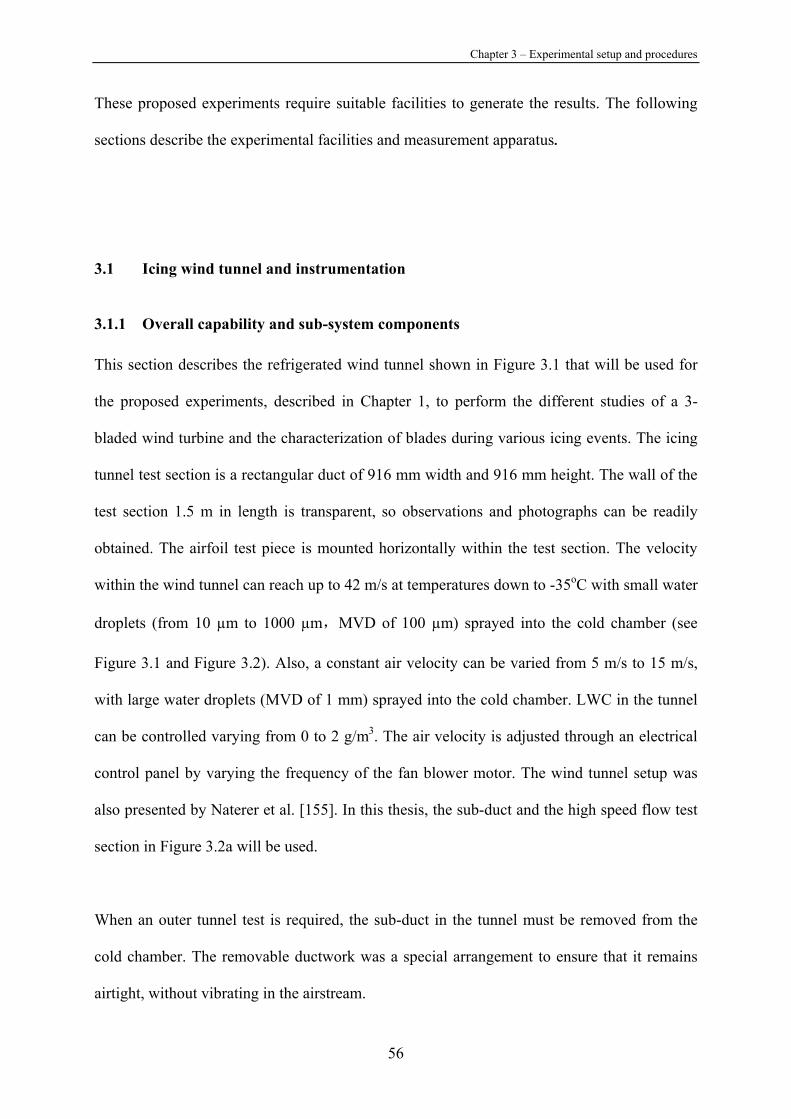
Chapter 3 – Experimental setup and procedures
56
These proposed experiments require suitable facilities to generate the results. The following
sections describe the experimental facilities and measurement apparatus.
3.1 Icing wind tunnel and instrumentation
3.1.1 Overall capability and sub-system components
This section describes the refrigerated wind tunnel shown in Figure 3.1 that will be used for
the proposed experiments, described in Chapter 1, to perform the different studies of a 3-
bladed wind turbine and the characterization of blades during various icing events. The icing
tunnel test section is a rectangular duct of 916 mm width and 916 mm height. The wall of the
test section 1.5 m in length is transparent, so observations and photographs can be readily
obtained. The airfoil test piece is mounted horizontally within the test section. The velocity
within the wind tunnel can reach up to 42 m/s at temperatures down to -35oC with small water
droplets (from 10 µm to 1000 µm,MVD of 100 µm) sprayed into the cold chamber (see
Figure 3.1 and Figure 3.2). Also, a constant air velocity can be varied from 5 m/s to 15 m/s,
with large water droplets (MVD of 1 mm) sprayed into the cold chamber. LWC in the tunnel
can be controlled varying from 0 to 2 g/m3. The air velocity is adjusted through an electrical
control panel by varying the frequency of the fan blower motor. The wind tunnel setup was
also presented by Naterer et al. [155]. In this thesis, the sub-duct and the high speed flow test
section in Figure 3.2a will be used.
When an outer tunnel test is required, the sub-duct in the tunnel must be removed from the
cold chamber. The removable ductwork was a special arrangement to ensure that it remains
airtight, without vibrating in the airstream.
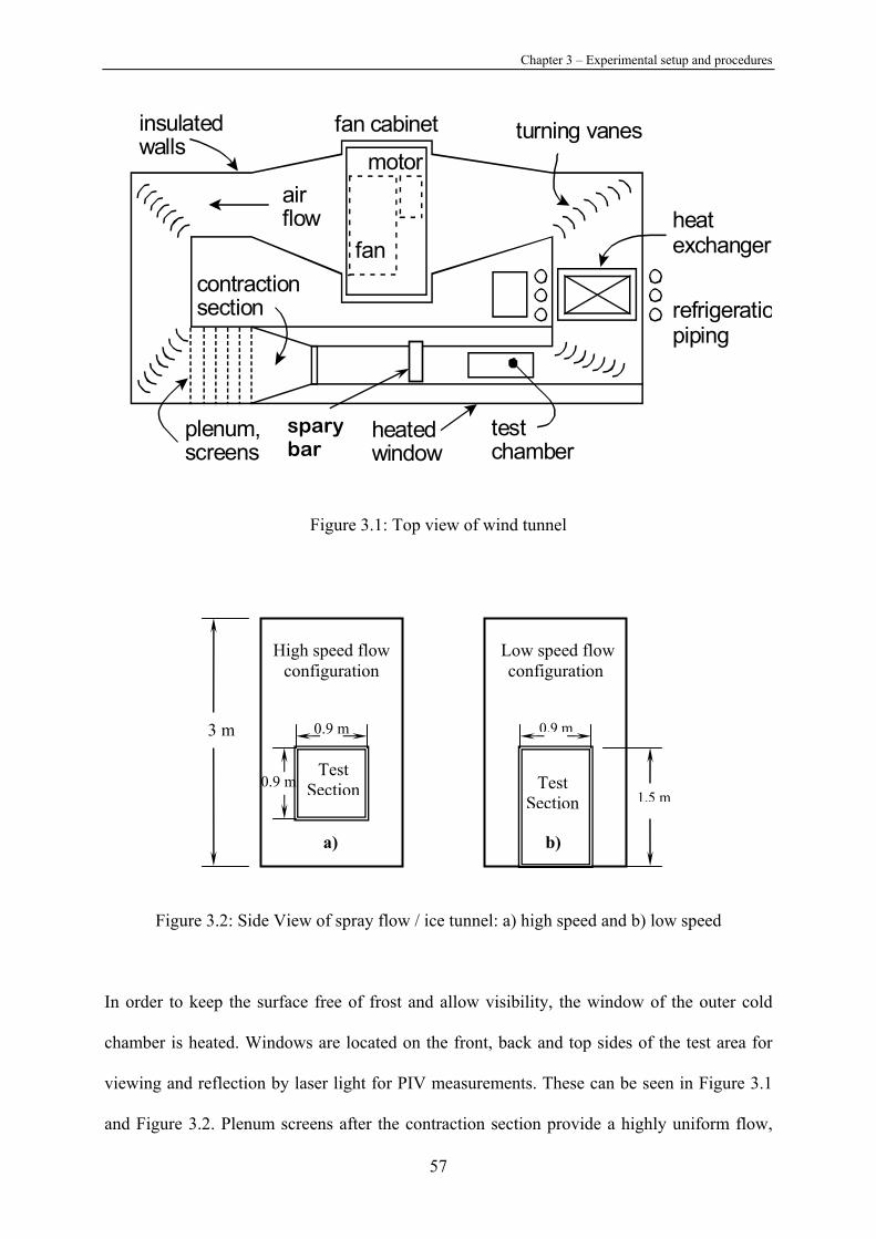
Chapter 3 – Experimental setup and procedures
57
Figure 3.1: Top view of wind tunnel
Figure 3.2: Side View of spray flow / ice tunnel: a) high speed and b) low speed
In order to keep the surface free of frost and allow visibility, the window of the outer cold
chamber is heated. Windows are located on the front, back and top sides of the test area for
viewing and reflection by laser light for PIV measurements. These can be seen in Figure 3.1
and Figure 3.2. Plenum screens after the contraction section provide a highly uniform flow,
1.5 m
0.9 m
High speed flow configuration
0.9 m
Low speed flow configuration
0.9 m Test Section Test
Section
3 m
b)a)
fan
motor
refrigeratiopiping
heatexchanger
plenum,screens
testchamber
heatedwindow
airflow
insulatedwalls
contractionsection
fan cabinet turning vanes
spary bar

Chapter 3 – Experimental setup and procedures
58
reaching the test section. The entire ductwork of the test section is removable to permit
different test sections for various test models. Doors are installed at various locations around
the perimeter of the icing tunnel to allow access inside for spray and test piece adjustments, as
well as cleaning of the ice after testing and regular maintenance of the various components.
Also, a de-icing system is built within the floors and tied into the compressors for
refrigeration of the icing tunnel.
Three evaporator heat exchanger systems are installed; each system can provide about 95,300
Btu per hour of cooling for a total capacity of 285,900 Btu per hour. The following systems
are components of the icing tunnel:
• Electronic control panels
• Oil separators
• Head pressure control
• Receiver inlet and outlet shutoff valves
• Service and safety relief valves
• Compressor contactor, pump down switch
• Control transformer
• Solid-state protection or internal lines break for compressor
• Recycle pump down cycle
The type of compressor is a Copalmetric 30 hp discus, single stage compressor designed for
refrigerant R422. The compressor housing is located in a separate room underneath the
laboratory. In addition, a defrost system is included to remove an ice buildup should it occur
during a test. The heater within the icing tunnel is designed to allow for a higher pressure drop,
due to ice buildup throughout the duration of the tests.

Chapter 3 – Experimental setup and procedures
59
3.1.2 Water spray system
There are many challenges to simulate natural icing conditions in a wind icing tunnel. A spray
bar is mounted in the refrigerated wind tunnel to simulate icing conditions. The spray bar is
designed with 4 nozzles in an aluminum streamlined shell. The spray bar is 910 mm long and
the nozzles are installed with a uniform spacing interval, in order to establish a uniform spray.
The shell of the spray bar is designed to contain the nozzles, as well as reduce large
magnitude disruptions to the airflow in the tunnel. The shape of the bar is a thin symmetrical
airfoil (152 mm wide wedge) with both ends rounded to reduce flow disturbances. Two
heating strips are installed between the nozzles and the aluminum shell to prevent the water
and nozzles from freezing during low temperature testing. The heating strips are resistive Ni-
Chrome wires embedded in a silicone jacket. They are heated by a variable power supply
using a 10 A transformer that can be adjusted from 0 to 120 V, thereby allowing variable
heating up to 1,200 Watts (see Figure 3.3). The operating condition of the spray bar is
monitored by a thermocouple mounted on one of the nozzles in the spray bar and the water
pipe section, through the wall of the wind tunnel. The spray bar was commissioned as part of
this research work.
Figure 3.3: Nozzle distribution with heaters and thermocouples inside the spray bar

Chapter 3 – Experimental setup and procedures
60
In order to reduce flow field disturbances at the outlet of the duct module within the tunnel,
where a test model will be set up, the spray bar is mounted 4,300 mm away from the outlet of
wind tunnel. This distance allows the water droplets to have sufficient time to form ice in a
low temperature environment. The flow to each nozzle is calibrated by controlling the
atomizing air flow. Calibrating the mass flow to each nozzle is time-consuming and it requires
adjustment of the valves until a uniform flow is obtained. Figure 3.4 shows the spray bar in
the wind tunnel.
Figure 3.4: Spray bar in the icing wind tunnel
Super-cooled water is supplied by a fluid system including a water tank, cooling compressor,
pump, temperature controller, water pressure controller, pipes and valves. The water
temperature can be set close to 0 degrees and the water pressure can be adjusted up to 70 psi.
Water flow is controlled by water valves and flow meters. Figure 3.5 shows the water flow-
meters and air pressure indicators with valves. Insulated foil is used to keep the water
temperature at cold levels. Also, an air filter, control key, manometer and cord for nozzle
heaters can be seen in Figure 3.5.
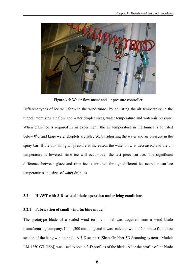
Chapter 3 – Experimental setup and procedures
61
Figure 3.5: Water flow meter and air pressure controller
Different types of ice will form in the wind tunnel by adjusting the air temperature in the
tunnel, atomizing air flow and water droplet sizes, water temperature and water/air pressure.
When glaze ice is required in an experiment, the air temperature in the tunnel is adjusted
below 0oC and large water droplets are selected, by adjusting the water and air pressure in the
spray bar. If the atomizing air pressure is increased, the water flow is decreased, and the air
temperature is lowered, rime ice will occur over the test piece surface. The significant
difference between glaze and rime ice is obtained through different ice accretion surface
temperatures and sizes of water droplets.
3.2 HAWT with 3-D twisted blade operation under icing conditions
3.2.1 Fabrication of small wind turbine model
The prototype blade of a scaled wind turbine model was acquired from a wind blade
manufacturing company. It is 1,300 mm long and it was scaled down to 420 mm to fit the test
section of the icing wind tunnel. A 3-D scanner (ShapeGrabber 3D Scanning systems, Model:
LM 1250 GT [156]) was used to obtain 3-D profiles of the blade. After the profile of the blade

Chapter 3 – Experimental setup and procedures
62
was scanned, all scanned data were merged together to form a digital blade. Merging the data
of the blade together was a challenge and it was very time consuming, because the blade is so
thin and the profile data obtained from the blade tip has little variation. Also, there are no
obvious characteristic points (used to identify the scanned object in reverse engineering) near
the tip of the blade. Figure 3.6b shows the blade after digitization (merged all scanned data
together) through Geomagic Studio [157] developed by the Raindrop Company, showing
flaws in the surface.
In order to manufacture the blade model, the rough profiles were smoothed to avoid faults in
the surface. Also, the blade centre was hollowed to reduce the weight of the blade using
Autodesk Inventor software. Specific sections from the digitized blade were chosen and then
flaws were modified in each airfoil. After all flaws were repaired, all airfoils were joined
together to form a whole blade. Figure 3.6a shows the blade after being processed by
Autodesk Inventor, which is the method used to fabricate each of the 3 blades, with a rapid
prototype machine. It uses resin to fabricate the model.
a) b) Figure 3.6: Digitized blade: a) smooth blade and b) blade before smoothing
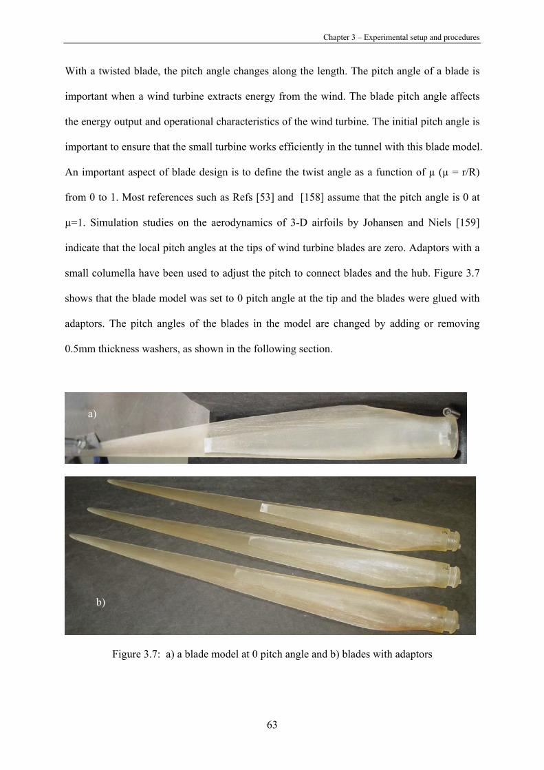
Chapter 3 – Experimental setup and procedures
63
With a twisted blade, the pitch angle changes along the length. The pitch angle of a blade is
important when a wind turbine extracts energy from the wind. The blade pitch angle affects
the energy output and operational characteristics of the wind turbine. The initial pitch angle is
important to ensure that the small turbine works efficiently in the tunnel with this blade model.
An important aspect of blade design is to define the twist angle as a function of µ (µ = r/R)
from 0 to 1. Most references such as Refs [53] and [158] assume that the pitch angle is 0 at
µ=1. Simulation studies on the aerodynamics of 3-D airfoils by Johansen and Niels [159]
indicate that the local pitch angles at the tips of wind turbine blades are zero. Adaptors with a
small columella have been used to adjust the pitch to connect blades and the hub. Figure 3.7
shows that the blade model was set to 0 pitch angle at the tip and the blades were glued with
adaptors. The pitch angles of the blades in the model are changed by adding or removing
0.5mm thickness washers, as shown in the following section.
Figure 3.7: a) a blade model at 0 pitch angle and b) blades with adaptors
a)
b)

Chapter 3 – Experimental setup and procedures
64
A hub was designed to connect the blades to the DC generator and also allow varying pitch
angles of each blade during an icing event. This aspect is important to the study, in order to
determine whether varying the pitch angles of the blades can help during various icing
conditions. Figure 3.8 shows the manufactured hub and hub centre. A set screw can be used to
change the pitch angle of the wind turbine blades by changing the position of the hub centre
with 0.5 mm washers (also shown in the figure). The brass hub has an 8-mm diameter hole to
accommodate the shaft of the generator.
a) b)
Figure 3.8: a) hub and b) hub center
The 3-D blades, hub and generator are assembled to construct a prototype wind turbine. The
washers between the hub centre and hub are able to adjust the pitch of the blades. The
washers were made from brass with 0.5 mm thickness and one can adjust the angles by 2.8°.
The 0 degree of the blade installation depends on the angle of the tip of the blade. Figure 3.9
shows the wind turbine working in the wind tunnel.
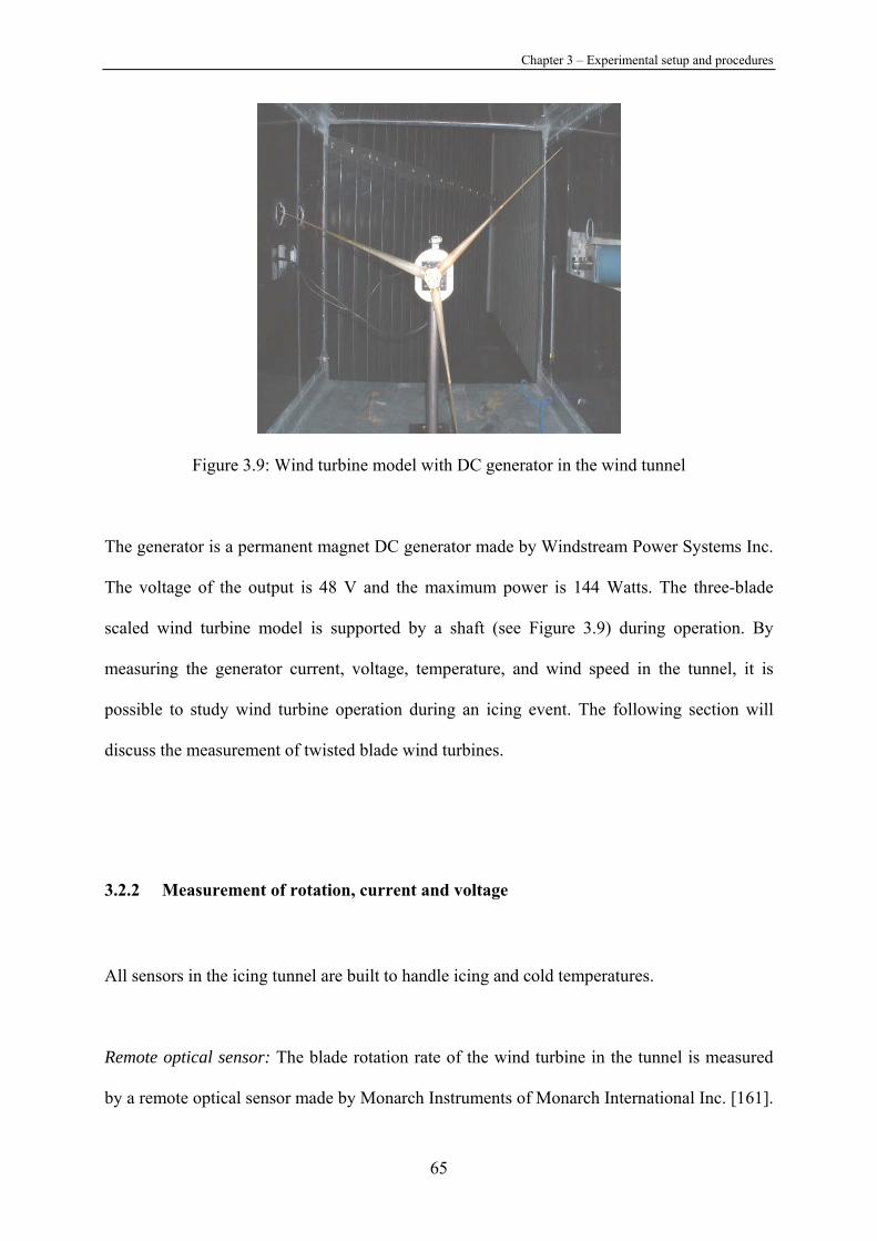
Chapter 3 – Experimental setup and procedures
65
Figure 3.9: Wind turbine model with DC generator in the wind tunnel
The generator is a permanent magnet DC generator made by Windstream Power Systems Inc.
The voltage of the output is 48 V and the maximum power is 144 Watts. The three-blade
scaled wind turbine model is supported by a shaft (see Figure 3.9) during operation. By
measuring the generator current, voltage, temperature, and wind speed in the tunnel, it is
possible to study wind turbine operation during an icing event. The following section will
discuss the measurement of twisted blade wind turbines.
3.2.2 Measurement of rotation, current and voltage
All sensors in the icing tunnel are built to handle icing and cold temperatures.
Remote optical sensor: The blade rotation rate of the wind turbine in the tunnel is measured
by a remote optical sensor made by Monarch Instruments of Monarch International Inc. [161].
Chapter 3 – Experimental setup and procedures
66
The sensor is capable of detecting a reflected pulse from a reflective tape target at distances
up to 1 m from a rotating object and angles up to 45 degrees. In the experiment, the sensor is
mounted on top of the wind tunnel at a distance of approximately 0.5 m from the shaft of the
wind turbine and a slight angle from the perpendicular direction. The lights are turned off, so
that only pulses from a reflective marker are received by the sensor. Water-proof reflective
tape is applied to a blade. Also, the sensor is optically aligned to illuminate the target once per
revolution. The green LEN On-Target indicator will blink at the input frequency rate when the
sensor is properly aimed. The sensor power requirement is 5 V DC, provided by Connector
Block SCB-100. The output from the sensor is a 0 - 5 V DC TTL pulse. It is connected to the
PCI-7033E data acquisition board via Connector Block SCB-100. The speed range of the
sensor (ROS-5 W) is 1~250,000 rpm and the operating temperature is -23°C to 121°C.
Transducers of current and voltage: The Series LTS current transducers are used to achieve a
total accuracy better than ±0.2% at 25°C. In contrast to the majority of closed-loop current
transducers available, the measuring resistor has been integrated into the transducer with an
accuracy of ±0.5% and a temperature drift of 50 ppm/K maximum [162]. In this experiment,
the LTS 6-NP is selected. This type of current transducer is a closed loop (compensated)
current transducer using the Hall Effect, unipolar voltage supply (+5 V from the Connector
Block SCB-100 box) and a compact design for PCB (Printed Circuit Board) mounting, which
incorporats a measuring range and extended measuring range. The primary nominal r.m.s.
current is 6 A, with a primary current measuring range of 0 ~ ±18 A and an analog output
voltage of 2.5 ±0.625 V that can be obtained by the PCI 6033E. We also can change the
measuring range for different connections in the transducer output side.
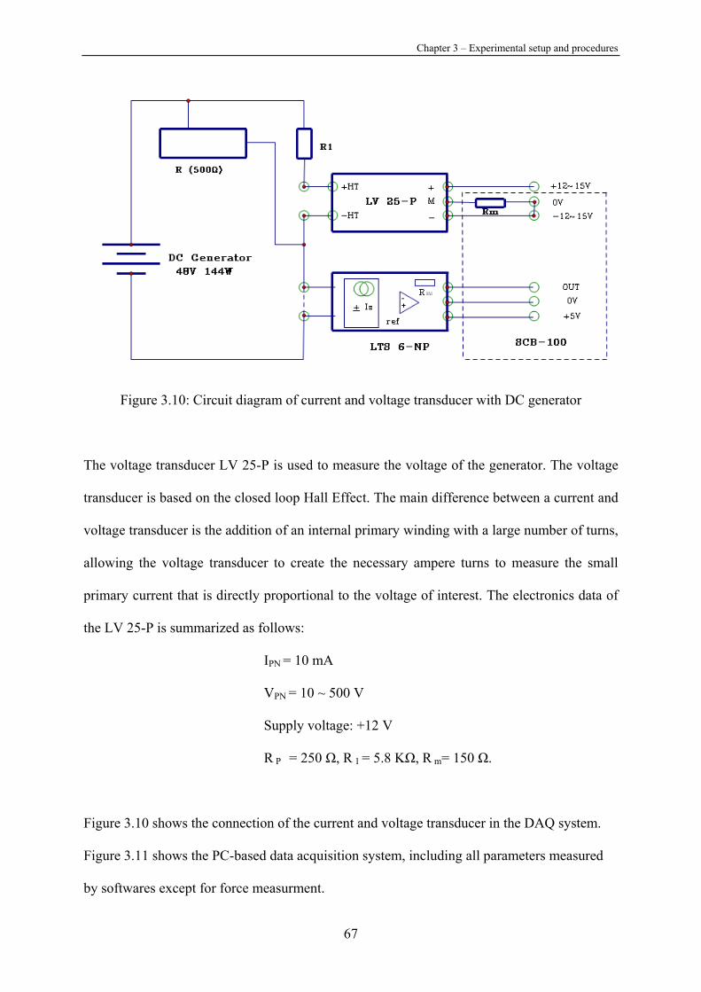
Chapter 3 – Experimental setup and procedures
67
Figure 3.10: Circuit diagram of current and voltage transducer with DC generator
The voltage transducer LV 25-P is used to measure the voltage of the generator. The voltage
transducer is based on the closed loop Hall Effect. The main difference between a current and
voltage transducer is the addition of an internal primary winding with a large number of turns,
allowing the voltage transducer to create the necessary ampere turns to measure the small
primary current that is directly proportional to the voltage of interest. The electronics data of
the LV 25-P is summarized as follows:
IPN = 10 mA
VPN = 10 ~ 500 V
Supply voltage: +12 V
R P = 250 Ω, R 1 = 5.8 KΩ, R m= 150 Ω.
Figure 3.10 shows the connection of the current and voltage transducer in the DAQ system.
Figure 3.11 shows the PC-based data acquisition system, including all parameters measured
by softwares except for force measurment.
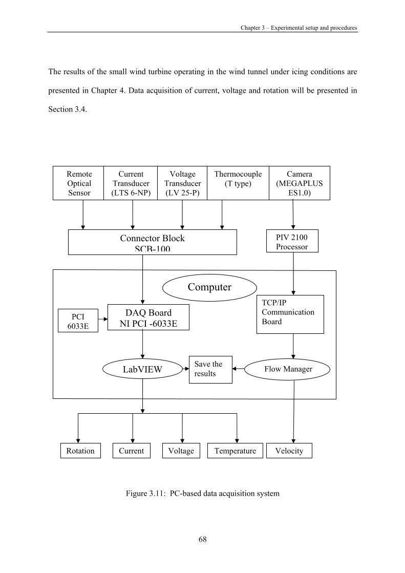
Chapter 3 – Experimental setup and procedures
68
The results of the small wind turbine operating in the wind tunnel under icing conditions are
presented in Chapter 4. Data acquisition of current, voltage and rotation will be presented in
Section 3.4.
Figure 3.11: PC-based data acquisition system
Remote Optical Sensor
Connector Block SCB-100
DAQ Board NI PCI -6033E
Current Transducer (LTS 6-NP)
Voltage Transducer (LV 25-P)
Thermocouple (T type)
PCI 6033E
Rotation Current Velocity Voltage Temperature
Save the results
TCP/IP Communication Board
PIV 2100 Processor
Camera (MEGAPLUS
ES1.0)
Computer
LabVIEW Flow Manager
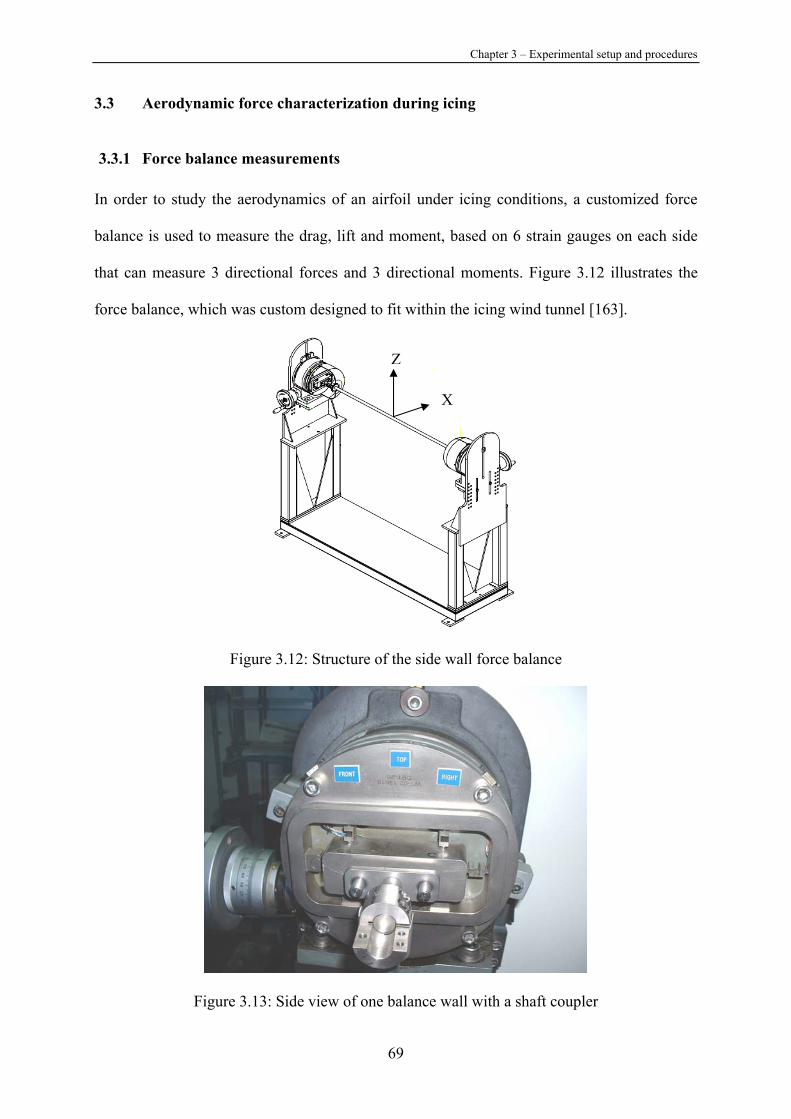
Chapter 3 – Experimental setup and procedures
69
3.3 Aerodynamic force characterization during icing
3.3.1 Force balance measurements
In order to study the aerodynamics of an airfoil under icing conditions, a customized force
balance is used to measure the drag, lift and moment, based on 6 strain gauges on each side
that can measure 3 directional forces and 3 directional moments. Figure 3.12 illustrates the
force balance, which was custom designed to fit within the icing wind tunnel [163].
Figure 3.12: Structure of the side wall force balance
Figure 3.13: Side view of one balance wall with a shaft coupler
X
Z
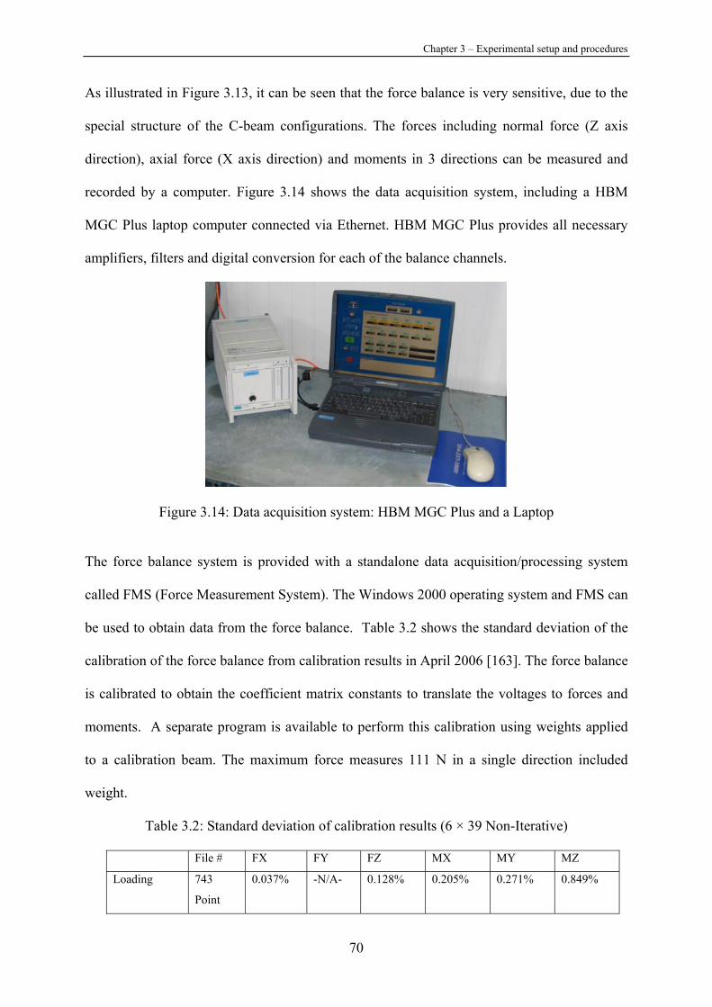
Chapter 3 – Experimental setup and procedures
70
As illustrated in Figure 3.13, it can be seen that the force balance is very sensitive, due to the
special structure of the C-beam configurations. The forces including normal force (Z axis
direction), axial force (X axis direction) and moments in 3 directions can be measured and
recorded by a computer. Figure 3.14 shows the data acquisition system, including a HBM
MGC Plus laptop computer connected via Ethernet. HBM MGC Plus provides all necessary
amplifiers, filters and digital conversion for each of the balance channels.
Figure 3.14: Data acquisition system: HBM MGC Plus and a Laptop
The force balance system is provided with a standalone data acquisition/processing system
called FMS (Force Measurement System). The Windows 2000 operating system and FMS can
be used to obtain data from the force balance. Table 3.2 shows the standard deviation of the
calibration of the force balance from calibration results in April 2006 [163]. The force balance
is calibrated to obtain the coefficient matrix constants to translate the voltages to forces and
moments. A separate program is available to perform this calibration using weights applied
to a calibration beam. The maximum force measures 111 N in a single direction included
weight.
Table 3.2: Standard deviation of calibration results (6 × 39 Non-Iterative)
File # FX FY FZ MX MY MZ
Loading 743
Point
0.037% -N/A- 0.128% 0.205% 0.271% 0.849%
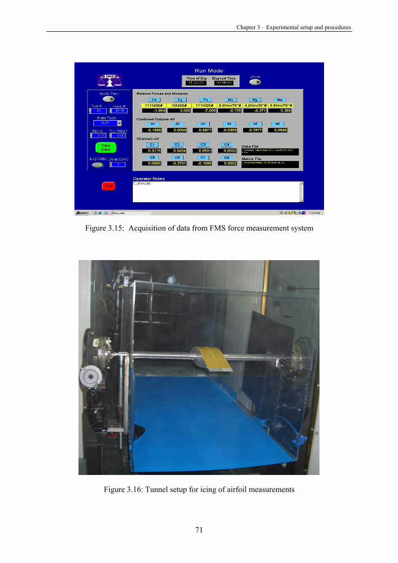
Chapter 3 – Experimental setup and procedures
71
Figure 3.15: Acquisition of data from FMS force measurement system
Figure 3.16: Tunnel setup for icing of airfoil measurements
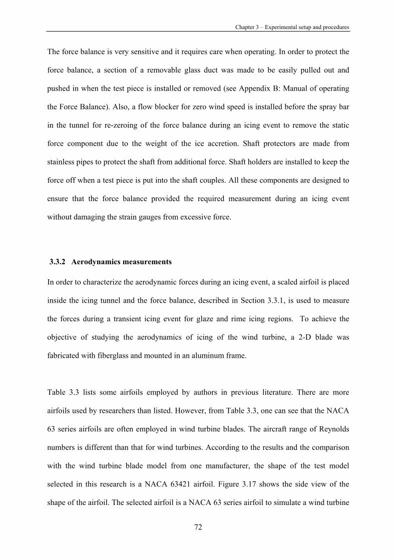
Chapter 3 – Experimental setup and procedures
72
The force balance is very sensitive and it requires care when operating. In order to protect the
force balance, a section of a removable glass duct was made to be easily pulled out and
pushed in when the test piece is installed or removed (see Appendix B: Manual of operating
the Force Balance). Also, a flow blocker for zero wind speed is installed before the spray bar
in the tunnel for re-zeroing of the force balance during an icing event to remove the static
force component due to the weight of the ice accretion. Shaft protectors are made from
stainless pipes to protect the shaft from additional force. Shaft holders are installed to keep the
force off when a test piece is put into the shaft couples. All these components are designed to
ensure that the force balance provided the required measurement during an icing event
without damaging the strain gauges from excessive force.
3.3.2 Aerodynamics measurements
In order to characterize the aerodynamic forces during an icing event, a scaled airfoil is placed
inside the icing tunnel and the force balance, described in Section 3.3.1, is used to measure
the forces during a transient icing event for glaze and rime icing regions. To achieve the
objective of studying the aerodynamics of icing of the wind turbine, a 2-D blade was
fabricated with fiberglass and mounted in an aluminum frame.
Table 3.3 lists some airfoils employed by authors in previous literature. There are more
airfoils used by researchers than listed. However, from Table 3.3, one can see that the NACA
63 series airfoils are often employed in wind turbine blades. The aircraft range of Reynolds
numbers is different than that for wind turbines. According to the results and the comparison
with the wind turbine blade model from one manufacturer, the shape of the test model
selected in this research is a NACA 63421 airfoil. Figure 3.17 shows the side view of the
shape of the airfoil. The selected airfoil is a NACA 63 series airfoil to simulate a wind turbine
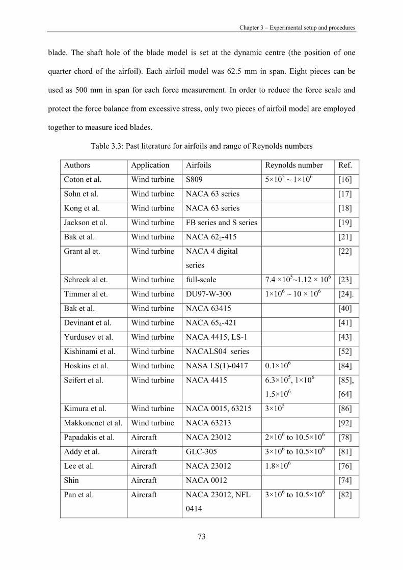
Chapter 3 – Experimental setup and procedures
73
blade. The shaft hole of the blade model is set at the dynamic centre (the position of one
quarter chord of the airfoil). Each airfoil model was 62.5 mm in span. Eight pieces can be
used as 500 mm in span for each force measurement. In order to reduce the force scale and
protect the force balance from excessive stress, only two pieces of airfoil model are employed
together to measure iced blades.
Table 3.3: Past literature for airfoils and range of Reynolds numbers
Authors Application Airfoils Reynolds number Ref.
Coton et al. Wind turbine S809 5×10⁵ ~ 1×10⁶ [16]
Sohn et al. Wind turbine NACA 63 series [17]
Kong et al. Wind turbine NACA 63 series [18]
Jackson et al. Wind turbine FB series and S series [19]
Bak et al. Wind turbine NACA 622-415 [21]
Grant al et. Wind turbine NACA 4 digital
series
[22]
Schreck al et. Wind turbine full-scale 7.4 ×10⁵~1.12 × 10⁶ [23]
Timmer al et. Wind turbine DU97-W-300 1×10⁶ ~ 10 × 106 [24].
Bak et al. Wind turbine NACA 63415 [40]
Devinant et al. Wind turbine NACA 654-421 [41]
Yurdusev et al. Wind turbine NACA 4415, LS-1 [43]
Kishinami et al. Wind turbine NACALS04 series [52]
Hoskins et al. Wind turbine NASA LS(1)-0417 0.1×10⁶ [84]
Seifert et al. Wind turbine NACA 4415 6.3×10⁵, 1×10⁶
1.5×10⁶
[85],
[64]
Kimura et al. Wind turbine NACA 0015, 63215 3×10⁵ [86]
Makkonenet et al. Wind turbine NACA 63213 [92]
Papadakis et al. Aircraft NACA 23012 2×10⁶ to 10.5×10⁶ [78]
Addy et al. Aircraft GLC-305 3×10⁶ to 10.5×10⁶ [81]
Lee et al. Aircraft NACA 23012 1.8×10⁶ [76]
Shin Aircraft NACA 0012 [74]
Pan et al. Aircraft NACA 23012, NFL
0414
3×10⁶ to 10.5×10⁶ [82]

Chapter 3 – Experimental setup and procedures
74
Test procedures: The wind tunnel air temperature is initially set. After a steady state has been
achieved, the force balance is zeroed to obtain the voltage offset, with no flow in the wind
tunnel. The LWC is then set and the air velocity set from a range from 0 to 35 m/s. Rime or
glaze ice is then simulated. During ice accretion, the forces are continuously measured. All
forces are checked to not damage the strain gauges of the force balance. Periodically the flow
in the tunnel is stopped to re-obtain a new zero offset to account for the added weight of the
ice.
Analysis: The measured aerodynamics of the airfoil is obtained by measuring the forces on
the airfoil under different conditions in the wind tunnel. Drag, lift and moment measurements
for the airfoil are achieved via the instruments described in Section 3.3.1.
The force balance can obtain the forces in the X and Z axis directions: FX and FZ. Also, the
angle of attack, α, can be set for an airfoil. The following equations can be used to obtain the
drag and lift forces.
αα sincos XZL FFF −= (3-1)
αα sincos ZXD FFF += (3-2)
The drag coefficient CD can be calculated as:
Lcu
FC DD 2
2
∞
=ρ
(3-3)
where FD is the mean drag force, ρ is the fluid density, L is the span of the airfoil and c is the
chord of the airfoil. The lift coefficient CL can be calculated as:
Lcu
FC L
L 2
2
∞
=ρ
(3-4)
where FL is the mean lift force.

Chapter 3 – Experimental setup and procedures
75
Preliminary results are shown in Chapter 5 for force measurements on a cylinder and a NACA
airfoil with various icing shapes.
3.4 Convective heat transfer characterization of wind blades
3.4.1 Setup of heat transfer for an airfoil
In order to characterize the convective heat transfer for wind blades during icing conditions,
three separate tests are performed, each corresponding to the three icing regions, as shown in
Table 3.4.
Table 3.4: Heat transfer and simulated icing conditions
Heat Transfer tests Icing Region Icing Condition Simulated
Airfoil in air Pre-icing This focuses on the single-phase convection
coefficient occurring before an icing event is
initiated. The convective heat transfer
coefficient variation from the leading edge of
the wind blade is required to be known,
especially when developing ice mitigation
techniques.
Airfoil in air and
water droplets (no
phase change)
Start of icing
conditions
Water droplets caused by precipitation start to
impact the blade surface and flow along the
blade. This region is composed of convection,
air with a known liquid content and water
partially covering the blade surface. Both
phases need to be tested.
Airfoil in air and
super-cooled droplets
with phase change
Post icing Water droplets have turned to rime or glaze ice
and more super-cooled water droplets are
deposited on the outer surface. The blade
profile has changed, impacting not only the
aerodynamics, but also the convective heat
transfer.

Chapter 3 – Experimental setup and procedures
76
Figure 3.17 shows the NACA 63421 airfoil used to perform these tests. The airfoil length and
width are 500 mm and 65 mm, respectively. The fiberglass airfoil has a wall thickness of
3 mm. This airfoil used for heat transfer characterization is fixed within an aluminum frame
and positioned in the icing wind tunnel using a vertical support bar that can be rotated to
change the pitch. T-type thermocouples are embedded at both inner and outer edges of the
airfoil surface. The thermocouple junctions are carefully flush-mounted with each surface at
several positions around the airfoil, as shown in Figure 3.17. The thermocouple lead wires are
collected within the hollow section of the airfoil and exit through the side of the airfoil. The
airfoil has 25 thermocouples mounted at various locations within the airfoil (see Figure 3.17),
including 22 thermocouples installed along the inner and outer surfaces of the airfoil.
Temperature differences between inner and outer surfaces are measured at 11 locations.
Heater strips are installed along the inner edges of the airfoil. The dimensions of the heating
strips are 40-mm in width and 880-mm in length. The operating voltage of the heating strip is
120 V and the power input is fixed at 500 W for all tests. The heater can be adjusted by a
variable transformer over a range of voltages from 0 V to 120 V. The heater strips are
attached inside of the airfoil with double-sided adhesive tape, after all thermocouples are
secured (see Figure 3.18: Test airfoil with a heater and thermocouples). The thermocouples
are connected to the data acquisition system of the icing tunnel, as described in Section 3.3.2.
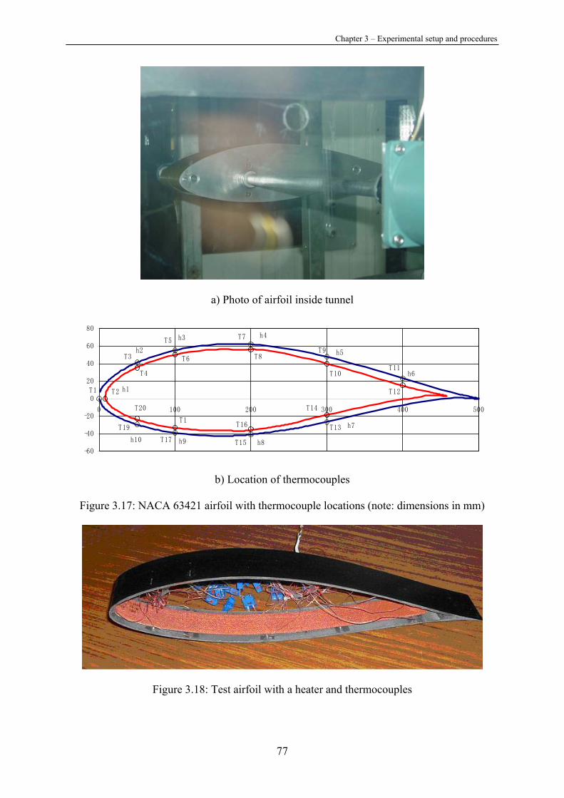
Chapter 3 – Experimental setup and procedures
77
a) Photo of airfoil inside tunnel
-60
-40
-20
0
20
40
60
80
0 100 200 300 400 500
T2
T8
T7
T4
T3
T1
T6
T5
T19
T11
T12
T10
T9
T1
T17
T16
T15
T14
T13
T20
h1
h10 h9 h8
h7
h6
h5
h4h3
h2
b) Location of thermocouples
Figure 3.17: NACA 63421 airfoil with thermocouple locations (note: dimensions in mm)
Figure 3.18: Test airfoil with a heater and thermocouples
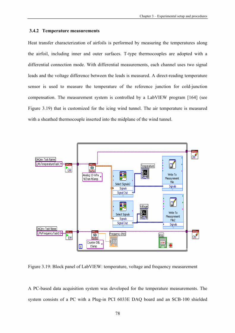
Chapter 3 – Experimental setup and procedures
78
3.4.2 Temperature measurements
Heat transfer characterization of airfoils is performed by measuring the temperatures along
the airfoil, including inner and outer surfaces. T-type thermocouples are adopted with a
differential connection mode. With differential measurements, each channel uses two signal
leads and the voltage difference between the leads is measured. A direct-reading temperature
sensor is used to measure the temperature of the reference junction for cold-junction
compensation. The measurement system is controlled by a LabVIEW program [164] (see
Figure 3.19) that is customized for the icing wind tunnel. The air temperature is measured
with a sheathed thermocouple inserted into the midplane of the wind tunnel.
Figure 3.19: Block panel of LabVIEW: temperature, voltage and frequency measurement
A PC-based data acquisition system was developed for the temperature measurements. The
system consists of a PC with a Plug-in PCI 6033E DAQ board and an SCB-100 shielded
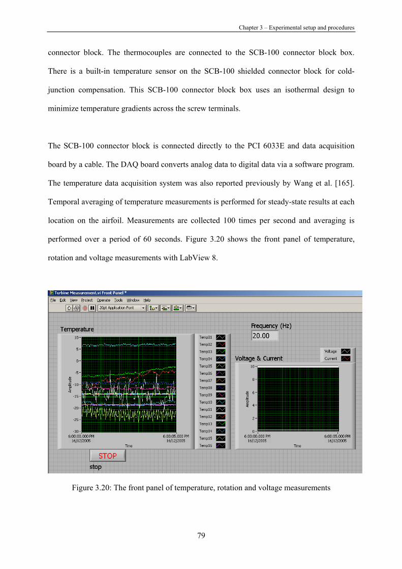
Chapter 3 – Experimental setup and procedures
79
connector block. The thermocouples are connected to the SCB-100 connector block box.
There is a built-in temperature sensor on the SCB-100 shielded connector block for cold-
junction compensation. This SCB-100 connector block box uses an isothermal design to
minimize temperature gradients across the screw terminals.
The SCB-100 connector block is connected directly to the PCI 6033E and data acquisition
board by a cable. The DAQ board converts analog data to digital data via a software program.
The temperature data acquisition system was also reported previously by Wang et al. [165].
Temporal averaging of temperature measurements is performed for steady-state results at each
location on the airfoil. Measurements are collected 100 times per second and averaging is
performed over a period of 60 seconds. Figure 3.20 shows the front panel of temperature,
rotation and voltage measurements with LabView 8.
Figure 3.20: The front panel of temperature, rotation and voltage measurements
Chapter 3 – Experimental setup and procedures
80
3.4.3 Test procedures and analysis
Test procedures: The test procedure consists of placing the airfoil inside the wind tunnel and
measuring the wind velocity, air temperature and wall temperatures. Water droplets are
injected to simulate the air-liquid tests. Experiments are performed for air temperatures
varying from -30oC to 20oC, wind speed from 5 m/s to 40 m/s and LWC from 0 to 2 g/m3 and
water droplet MVD rangs from 10 µm to 1000 µm.
Analysis: Spatial averaging of heat transfer coefficients is performed to obtain the average
Nusselt number. Temperature measurements recorded at various locations around the NACA
airfoil are used to determine the convective heat transfer coefficient. The rate of convective
heat transfer per unit area from the airfoil is determined by:
)( ocon TThq −= ∞ (3-5)
which can be re-arranged to give
con
o
qhT T∞
=− (3-6)
Heater strips below the airfoil surface provide a source of heat input, which is transported
through the thin airfoil surface by conduction, then convection to the external air stream. Heat
conduction perpendicular to the surface is much larger than lateral heat conduction due to the
high temperature difference across the thin surface. The perpendicular Fourier heat flux
balances the rate of convective heat transfer to the surrounding air stream, i.e.,
( )in ocon cd
k T Tq qδ−
= = (3-7)
Substituting Eq. 3-7 into Eq. 3-6, the resulting heat transfer coefficient can be expressed in the
following manner,
Chapter 3 – Experimental setup and procedures
81
( )( )
in o
o
k T ThT Tδ ∞
−=
− (3-8)
The average heat transfer coefficient was obtained from spatial averaging around the airfoil.
∑∫ ∆==1111i
iis
shs
hdxs
h (3-9)
Then, the average Nusselt number becomes
airkchNu = (3-10)
The results are presented in Chapter 6 for both average and local Nusselt numbers under the
following test conditions:
1. Heat transfer from the airfoil without droplets for air temperatures ranging from -30oC to
20oC at AOA = 0;
2. Heat transfer from the airfoil with droplets having the same temperature as the air with
different liquid water contents at AOA = 0;
3. Heat transfer from the airfoil without droplets for temperatures ranging from -30oC to
20oC at varying AOA;
4. Heat transfer from the airfoil with droplets having the same temperature of the air with
different liquid water contents at various AOA.
Chapter 6 will provide the detailed results.
This chapter has presented the wind tunnel facility at the University of Manitoba and
experimental instruments, including the force balance and thermocouples installed in the
airfoil. The following aspects are covered in upcoming chapters.
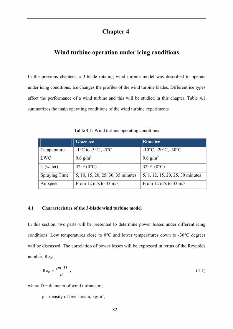
82
Chapter 4
Wind turbine operation under icing conditions
In the previous chapters, a 3-blade rotating wind turbine model was described to operate
under icing conditions. Ice changes the profiles of the wind turbine blades. Different ice types
affect the performance of a wind turbine and this will be studied in this chapter. Table 4.1
summarizes the main operating conditions of the wind turbine experiments.
Table 4.1: Wind turbine operating conditions
Glaze ice Rime ice
Temperature -1°C to -3°C , -5°C -10°C, -20°C, -30°C
LWC 0.6 g/m3 0.6 g/m3
T (water) 32°F (0°C) 32°F (0°C)
Spraying Time 5, 10, 15, 20, 25, 30, 35 minutes 5, 8, 12, 15, 20, 25, 30 minutes
Air speed From 12 m/s to 33 m/s From 12 m/s to 33 m/s
4.1 Characteristics of the 3-blade wind turbine model
In this section, two parts will be presented to determine power losses under different icing
conditions. Low temperatures close to 0°C and lower temperatures down to -30°C degrees
will be discussed. The correlation of power losses will be expressed in terms of the Reynolds
number, ReD:
µρ Du
D∞=Re , (4-1)
where D = diameter of wind turbine, m,
ρ = density of free stream, kg/m3,
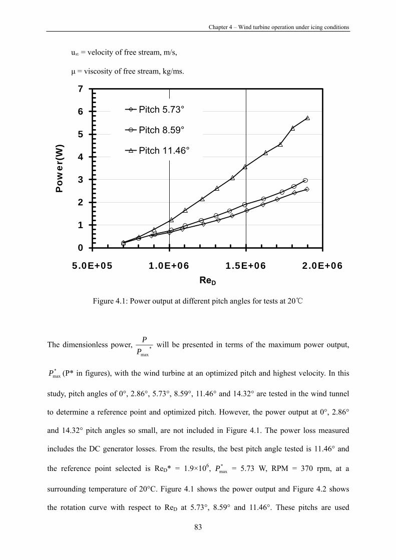
Chapter 4 – Wind turbine operation under icing conditions
83
u∞ = velocity of free stream, m/s,
µ = viscosity of free stream, kg/ms.
0
1
2
3
4
5
6
7
5.0E+05 1.0E+06 1.5E+06 2.0E+06ReD
Pow
er(W
)
Pitch 5.73°
Pitch 8.59°
Pitch 11.46°
Figure 4.1: Power output at different pitch angles for tests at 20
The dimensionless power, *maxPP will be presented in terms of the maximum power output,
*maxP (P* in figures), with the wind turbine at an optimized pitch and highest velocity. In this
study, pitch angles of 0°, 2.86°, 5.73°, 8.59°, 11.46° and 14.32° are tested in the wind tunnel
to determine a reference point and optimized pitch. However, the power output at 0°, 2.86°
and 14.32° pitch angles so small, are not included in Figure 4.1. The power loss measured
includes the DC generator losses. From the results, the best pitch angle tested is 11.46° and
the reference point selected is ReD* = 1.9×10⁶, *maxP = 5.73 W, RPM = 370 rpm, at a
surrounding temperature of 20°C. Figure 4.1 shows the power output and Figure 4.2 shows
the rotation curve with respect to ReD at 5.73°, 8.59° and 11.46°. These pitchs are used
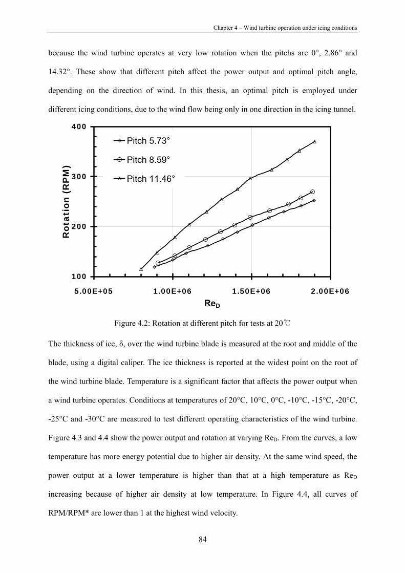
Chapter 4 – Wind turbine operation under icing conditions
84
because the wind turbine operates at very low rotation when the pitchs are 0°, 2.86° and
14.32°. These show that different pitch affect the power output and optimal pitch angle,
depending on the direction of wind. In this thesis, an optimal pitch is employed under
different icing conditions, due to the wind flow being only in one direction in the icing tunnel.
100
200
300
400
5.00E+05 1.00E+06 1.50E+06 2.00E+06ReD
Rot
atio
n (R
PM
)
Pitch 5.73°
Pitch 8.59°
Pitch 11.46°
Figure 4.2: Rotation at different pitch for tests at 20
The thickness of ice, δ, over the wind turbine blade is measured at the root and middle of the
blade, using a digital caliper. The ice thickness is reported at the widest point on the root of
the wind turbine blade. Temperature is a significant factor that affects the power output when
a wind turbine operates. Conditions at temperatures of 20°C, 10°C, 0°C, -10°C, -15°C, -20°C,
-25°C and -30°C are measured to test different operating characteristics of the wind turbine.
Figure 4.3 and 4.4 show the power output and rotation at varying ReD. From the curves, a low
temperature has more energy potential due to higher air density. At the same wind speed, the
power output at a lower temperature is higher than that at a high temperature as ReD
increasing because of higher air density at low temperature. In Figure 4.4, all curves of
RPM/RPM* are lower than 1 at the highest wind velocity.
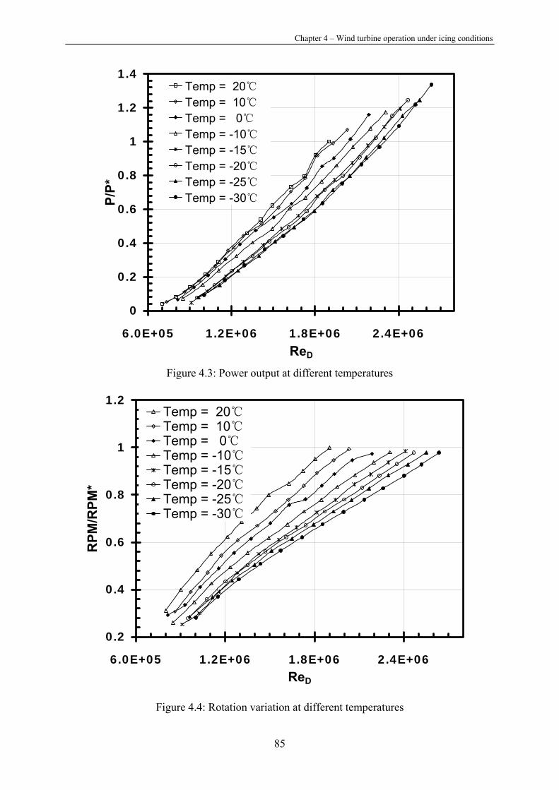
Chapter 4 – Wind turbine operation under icing conditions
85
0
0.2
0.4
0.6
0.8
1
1.2
1.4
6.0E+05 1.2E+06 1.8E+06 2.4E+06ReD
P/P*
Temp = 20Temp = 10Temp = 0Temp = -10Temp = -15Temp = -20Temp = -25Temp = -30
Figure 4.3: Power output at different temperatures
0.2
0.4
0.6
0.8
1
1.2
6.0E+05 1.2E+06 1.8E+06 2.4E+06ReD
RPM
/RPM
*
Temp = 20Temp = 10Temp = 0Temp = -10Temp = -15Temp = -20Temp = -25Temp = -30
Figure 4.4: Rotation variation at different temperatures
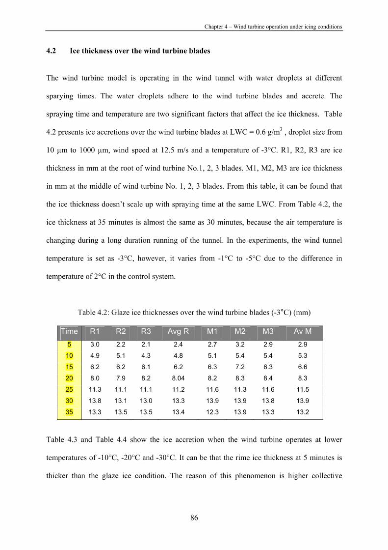
Chapter 4 – Wind turbine operation under icing conditions
86
4.2 Ice thickness over the wind turbine blades
The wind turbine model is operating in the wind tunnel with water droplets at different
sparying times. The water droplets adhere to the wind turbine blades and accrete. The
spraying time and temperature are two significant factors that affect the ice thickness. Table
4.2 presents ice accretions over the wind turbine blades at LWC = 0.6 g/m3 , droplet size from
10 µm to 1000 µm, wind speed at 12.5 m/s and a temperature of -3°C. R1, R2, R3 are ice
thickness in mm at the root of wind turbine No.1, 2, 3 blades. M1, M2, M3 are ice thickness
in mm at the middle of wind turbine No. 1, 2, 3 blades. From this table, it can be found that
the ice thickness doesn’t scale up with spraying time at the same LWC. From Table 4.2, the
ice thickness at 35 minutes is almost the same as 30 minutes, because the air temperature is
changing during a long duration running of the tunnel. In the experiments, the wind tunnel
temperature is set as -3°C, however, it varies from -1°C to -5°C due to the difference in
temperature of 2°C in the control system.
Table 4.2: Glaze ice thicknesses over the wind turbine blades (-3°C) (mm)
Time R1 R2 R3 Avg R M1 M2 M3 Av M 5 3.0 2.2 2.1 2.4 2.7 3.2 2.9 2.9
10 4.9 5.1 4.3 4.8 5.1 5.4 5.4 5.3
15 6.2 6.2 6.1 6.2 6.3 7.2 6.3 6.6
20 8.0 7.9 8.2 8.04 8.2 8.3 8.4 8.3
25 11.3 11.1 11.1 11.2 11.6 11.3 11.6 11.5
30 13.8 13.1 13.0 13.3 13.9 13.9 13.8 13.9
35 13.3 13.5 13.5 13.4 12.3 13.9 13.3 13.2
Table 4.3 and Table 4.4 show the ice accretion when the wind turbine operates at lower
temperatures of -10°C, -20°C and -30°C. It can be that the rime ice thickness at 5 minutes is
thicker than the glaze ice condition. The reason of this phenomenon is higher collective
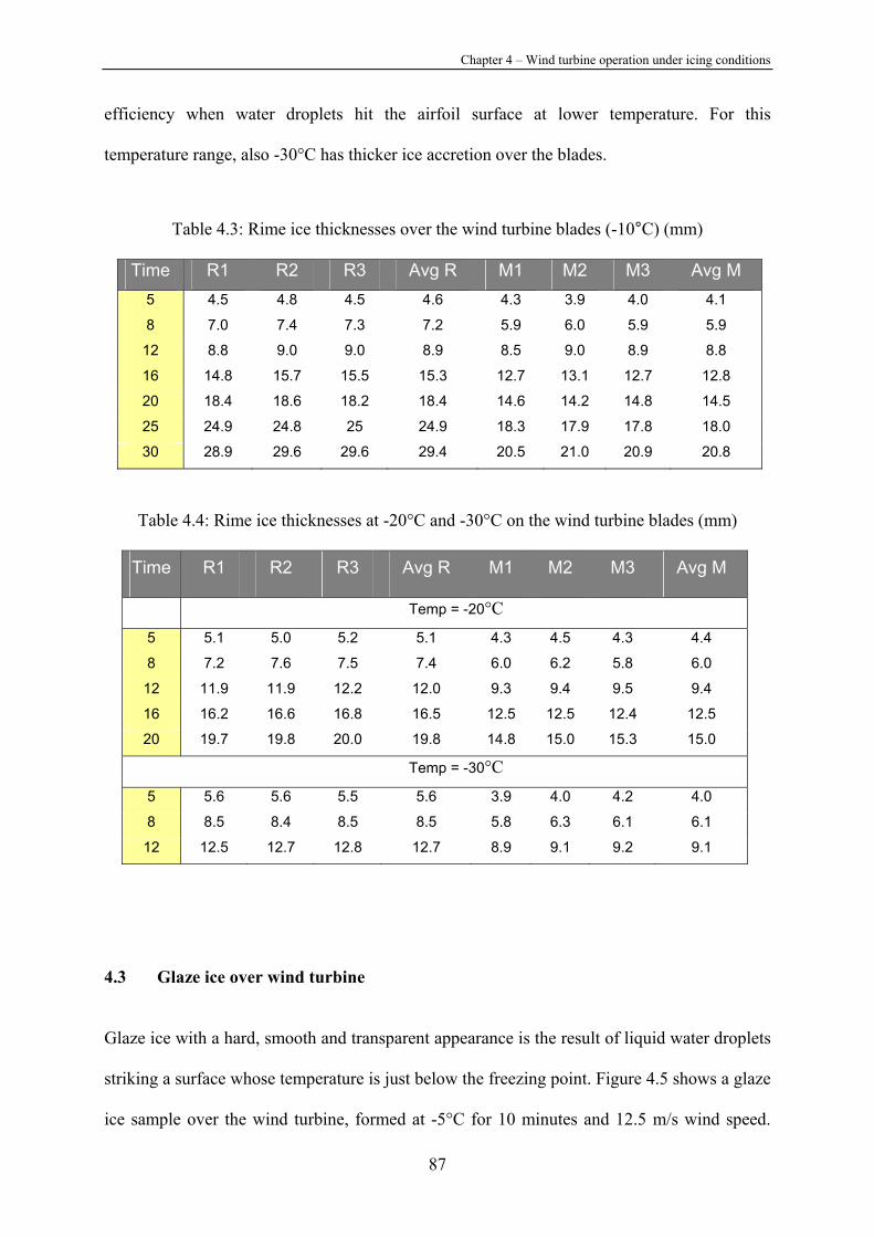
Chapter 4 – Wind turbine operation under icing conditions
87
efficiency when water droplets hit the airfoil surface at lower temperature. For this
temperature range, also -30°C has thicker ice accretion over the blades.
Table 4.3: Rime ice thicknesses over the wind turbine blades (-10°C) (mm)
Time R1 R2 R3 Avg R M1 M2 M3 Avg M 5 4.5 4.8 4.5 4.6 4.3 3.9 4.0 4.1
8 7.0 7.4 7.3 7.2 5.9 6.0 5.9 5.9
12 8.8 9.0 9.0 8.9 8.5 9.0 8.9 8.8
16 14.8 15.7 15.5 15.3 12.7 13.1 12.7 12.8
20 18.4 18.6 18.2 18.4 14.6 14.2 14.8 14.5
25 24.9 24.8 25 24.9 18.3 17.9 17.8 18.0
30 28.9 29.6 29.6 29.4 20.5 21.0 20.9 20.8
Table 4.4: Rime ice thicknesses at -20°C and -30°C on the wind turbine blades (mm)
Time R1 R2 R3 Avg R M1 M2 M3 Avg M
Temp = -20°C
5 5.1 5.0 5.2 5.1 4.3 4.5 4.3 4.4
8 7.2 7.6 7.5 7.4 6.0 6.2 5.8 6.0
12 11.9 11.9 12.2 12.0 9.3 9.4 9.5 9.4
16 16.2 16.6 16.8 16.5 12.5 12.5 12.4 12.5
20 19.7 19.8 20.0 19.8 14.8 15.0 15.3 15.0
Temp = -30°C
5 5.6 5.6 5.5 5.6 3.9 4.0 4.2 4.0
8 8.5 8.4 8.5 8.5 5.8 6.3 6.1 6.1
12 12.5 12.7 12.8 12.7 8.9 9.1 9.2 9.1
4.3 Glaze ice over wind turbine
Glaze ice with a hard, smooth and transparent appearance is the result of liquid water droplets
striking a surface whose temperature is just below the freezing point. Figure 4.5 shows a glaze
ice sample over the wind turbine, formed at -5°C for 10 minutes and 12.5 m/s wind speed.
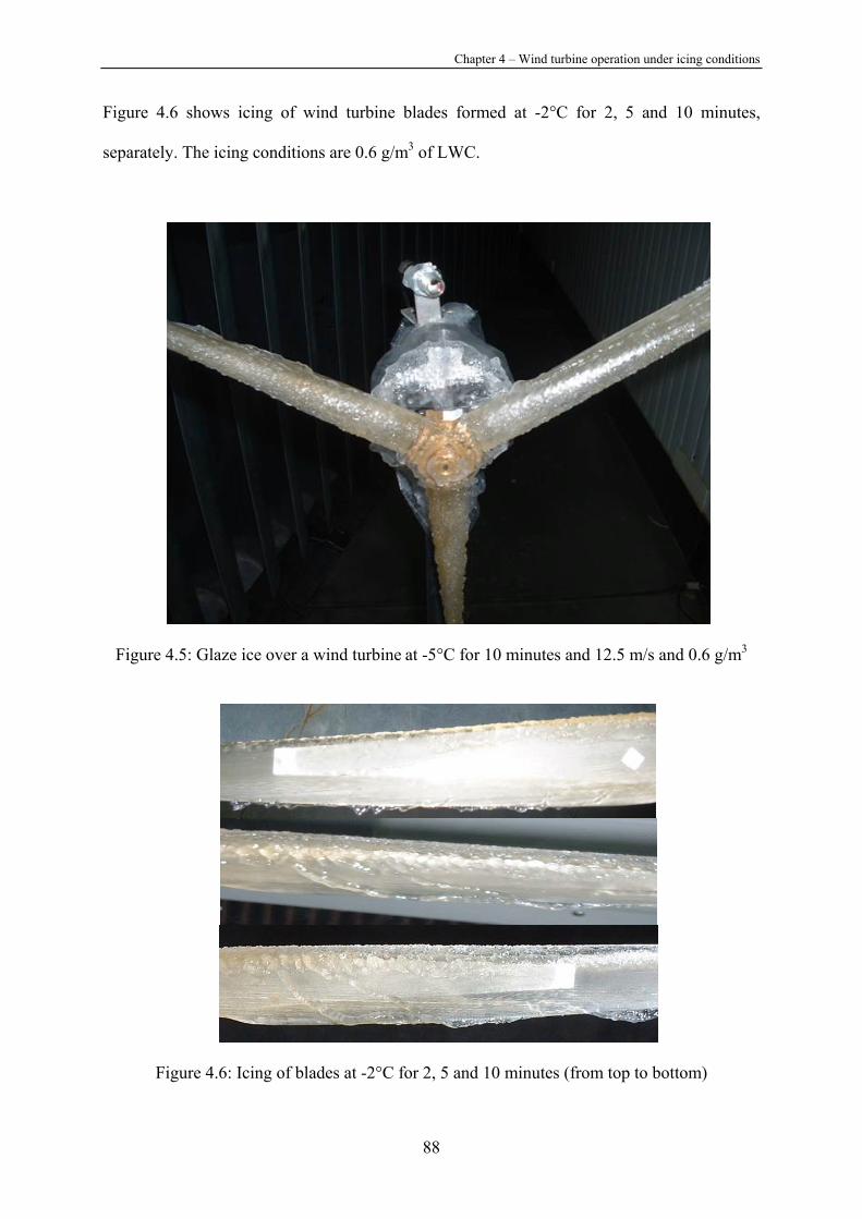
Chapter 4 – Wind turbine operation under icing conditions
88
Figure 4.6 shows icing of wind turbine blades formed at -2°C for 2, 5 and 10 minutes,
separately. The icing conditions are 0.6 g/m3 of LWC.
Figure 4.5: Glaze ice over a wind turbine at -5°C for 10 minutes and 12.5 m/s and 0.6 g/m3
Figure 4.6: Icing of blades at -2°C for 2, 5 and 10 minutes (from top to bottom)
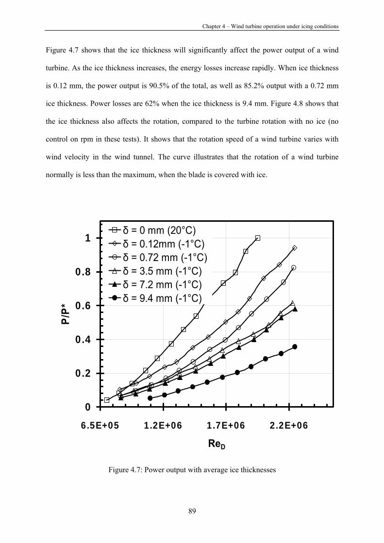
Chapter 4 – Wind turbine operation under icing conditions
89
Figure 4.7 shows that the ice thickness will significantly affect the power output of a wind
turbine. As the ice thickness increases, the energy losses increase rapidly. When ice thickness
is 0.12 mm, the power output is 90.5% of the total, as well as 85.2% output with a 0.72 mm
ice thickness. Power losses are 62% when the ice thickness is 9.4 mm. Figure 4.8 shows that
the ice thickness also affects the rotation, compared to the turbine rotation with no ice (no
control on rpm in these tests). It shows that the rotation speed of a wind turbine varies with
wind velocity in the wind tunnel. The curve illustrates that the rotation of a wind turbine
normally is less than the maximum, when the blade is covered with ice.
0
0.2
0.4
0.6
0.8
1
6.5E+05 1.2E+06 1.7E+06 2.2E+06
ReD
P/P*
δ = 0 mm (20°C)δ = 0.12mm (-1°C)δ = 0.72 mm (-1°C)δ = 3.5 mm (-1°C)δ = 7.2 mm (-1°C)δ = 9.4 mm (-1°C)
Figure 4.7: Power output with average ice thicknesses
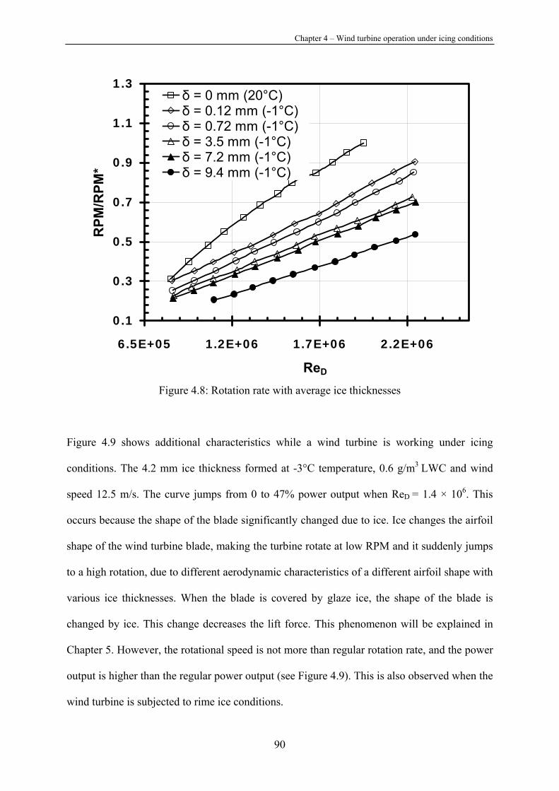
Chapter 4 – Wind turbine operation under icing conditions
90
0.1
0.3
0.5
0.7
0.9
1.1
1.3
6.5E+05 1.2E+06 1.7E+06 2.2E+06
ReD
RPM
/RPM
*δ = 0 mm (20°C)δ = 0.12 mm (-1°C)δ = 0.72 mm (-1°C)δ = 3.5 mm (-1°C)δ = 7.2 mm (-1°C)δ = 9.4 mm (-1°C)
Figure 4.8: Rotation rate with average ice thicknesses
Figure 4.9 shows additional characteristics while a wind turbine is working under icing
conditions. The 4.2 mm ice thickness formed at -3°C temperature, 0.6 g/m3 LWC and wind
speed 12.5 m/s. The curve jumps from 0 to 47% power output when ReD = 1.4 × 10⁶. This
occurs because the shape of the blade significantly changed due to ice. Ice changes the airfoil
shape of the wind turbine blade, making the turbine rotate at low RPM and it suddenly jumps
to a high rotation, due to different aerodynamic characteristics of a different airfoil shape with
various ice thicknesses. When the blade is covered by glaze ice, the shape of the blade is
changed by ice. This change decreases the lift force. This phenomenon will be explained in
Chapter 5. However, the rotational speed is not more than regular rotation rate, and the power
output is higher than the regular power output (see Figure 4.9). This is also observed when the
wind turbine is subjected to rime ice conditions.

Chapter 4 – Wind turbine operation under icing conditions
91
0
0.2
0.4
0.6
0.8
1
6.5E+05 1.2E+06 1.7E+06 2.2E+06
ReD
P/P*
0
0.2
0.4
0.6
0.8
1
RPM
/RPM
*
δ = 0 mm (20°C) P δ = 4.2 mm (-3°C) Pδ = 0 mm (20°C) RPM δ = 4.2 mm (-3°C) RPM
Figure 4.9: Power output for a 4.2 mm average ice thickness
4.4 Power losses with rime iced blades
Rime ice has a rough and opaque appearance and it forms when the surface temperature is
below the freezing point and exposed to super-cooled water droplets. Due to the presence of
trapped air bubbles, rime ice is opaque and its density ranges from 0.59 to 0.9 g/cm3,
depending on accretion conditions. Figure 4.10 shows an example of rime ice on the wind
turbine and blades.
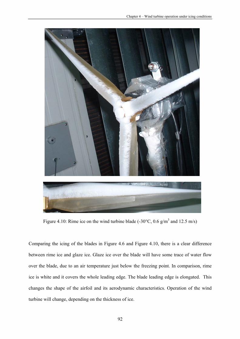
Chapter 4 – Wind turbine operation under icing conditions
92
Figure 4.10: Rime ice on the wind turbine blade (-30°C, 0.6 g/m3 and 12.5 m/s)
Comparing the icing of the blades in Figure 4.6 and Figure 4.10, there is a clear difference
between rime ice and glaze ice. Glaze ice over the blade will have some trace of water flow
over the blade, due to an air temperature just below the freezing point. In comparison, rime
ice is white and it covers the whole leading edge. The blade leading edge is elongated. This
changes the shape of the airfoil and its aerodynamic characteristics. Operation of the wind
turbine will change, depending on the thickness of ice.
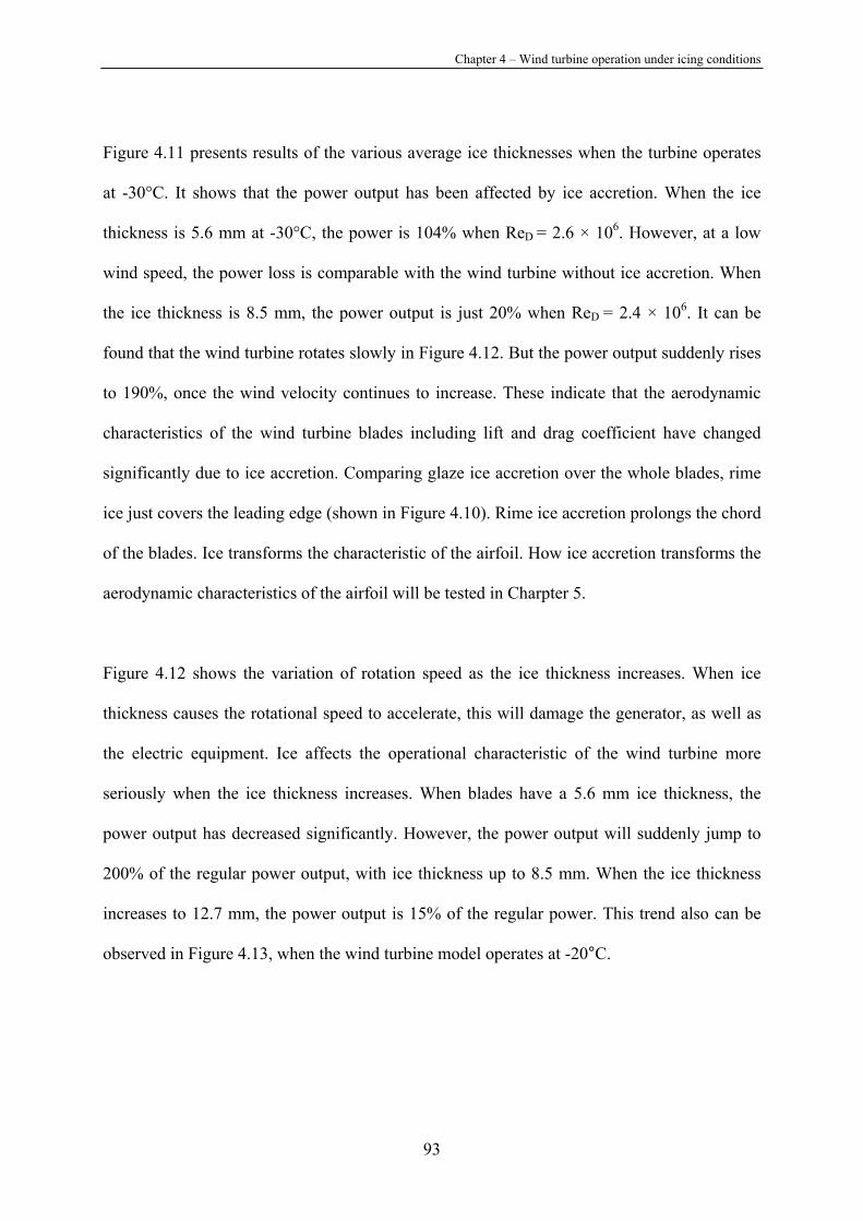
Chapter 4 – Wind turbine operation under icing conditions
93
Figure 4.11 presents results of the various average ice thicknesses when the turbine operates
at -30°C. It shows that the power output has been affected by ice accretion. When the ice
thickness is 5.6 mm at -30°C, the power is 104% when ReD = 2.6 × 10⁶. However, at a low
wind speed, the power loss is comparable with the wind turbine without ice accretion. When
the ice thickness is 8.5 mm, the power output is just 20% when ReD = 2.4 × 10⁶. It can be
found that the wind turbine rotates slowly in Figure 4.12. But the power output suddenly rises
to 190%, once the wind velocity continues to increase. These indicate that the aerodynamic
characteristics of the wind turbine blades including lift and drag coefficient have changed
significantly due to ice accretion. Comparing glaze ice accretion over the whole blades, rime
ice just covers the leading edge (shown in Figure 4.10). Rime ice accretion prolongs the chord
of the blades. Ice transforms the characteristic of the airfoil. How ice accretion transforms the
aerodynamic characteristics of the airfoil will be tested in Charpter 5.
Figure 4.12 shows the variation of rotation speed as the ice thickness increases. When ice
thickness causes the rotational speed to accelerate, this will damage the generator, as well as
the electric equipment. Ice affects the operational characteristic of the wind turbine more
seriously when the ice thickness increases. When blades have a 5.6 mm ice thickness, the
power output has decreased significantly. However, the power output will suddenly jump to
200% of the regular power output, with ice thickness up to 8.5 mm. When the ice thickness
increases to 12.7 mm, the power output is 15% of the regular power. This trend also can be
observed in Figure 4.13, when the wind turbine model operates at -20°C.
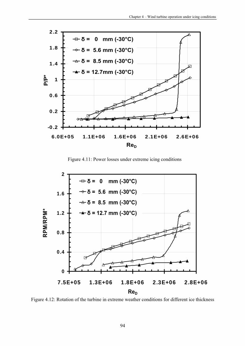
Chapter 4 – Wind turbine operation under icing conditions
94
-0.2
0.2
0.6
1
1.4
1.8
2.2
6.0E+05 1.1E+06 1.6E+06 2.1E+06 2.6E+06ReD
P/P*
δ = 0 mm (-30°C)
δ = 5.6 mm (-30°C)
δ = 8.5 mm (-30°C)
δ = 12.7mm (-30°C)
Figure 4.11: Power losses under extreme icing conditions
0
0.4
0.8
1.2
1.6
2
7.5E+05 1.3E+06 1.8E+06 2.3E+06 2.8E+06ReD
RPM
/RPM
*
δ = 0 mm (-30°C)
δ = 5.6 mm (-30°C)
δ = 8.5 mm (-30°C)
δ = 12.7 mm (-30°C)
Figure 4.12: Rotation of the turbine in extreme weather conditions for different ice thickness
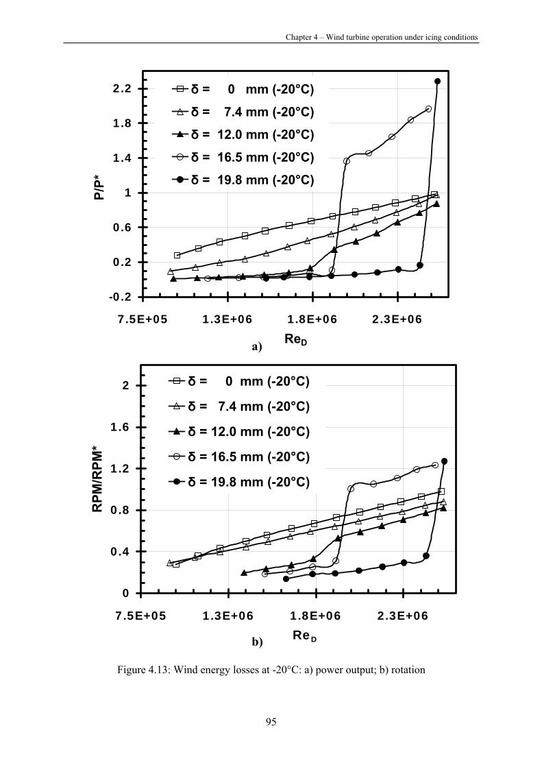
Chapter 4 – Wind turbine operation under icing conditions
95
-0.2
0.2
0.6
1
1.4
1.8
2.2
7.5E+05 1.3E+06 1.8E+06 2.3E+06ReD
P/P*
δ = 0 mm (-20°C)
δ = 7.4 mm (-20°C)
δ = 12.0 mm (-20°C)
δ = 16.5 mm (-20°C)
δ = 19.8 mm (-20°C)
0
0.4
0.8
1.2
1.6
2
7.5E+05 1.3E+06 1.8E+06 2.3E+06
ReD
RPM
/RPM
*
δ = 0 mm (-20°C)
δ = 7.4 mm (-20°C)
δ = 12.0 mm (-20°C)
δ = 16.5 mm (-20°C)
δ = 19.8 mm (-20°C)
Figure 4.13: Wind energy losses at -20°C: a) power output; b) rotation
a)
b) ReD

Chapter 4 – Wind turbine operation under icing conditions
96
Figure 4.13 shows that the power output changes with different ice thicknesses at -20°C.
Compared with -30°C, the ice thickness of the wind turbine blades is thicker, while the power
output suddenly jumps to a higher power output at the lower wind velocity. When ice accretes
over the blades, 19.8 mm of ice thickness leads to a transition at ReD = 2.5 × 10⁶. Ice accretion
creates different ice shapes at different temperatures. Various ice shapes affects the lift
coefficient in different way.
4.5 Summary
The experimental results in this chapters showed that icing of a wind turbine blade
significantly affects energy output, regardless of what kind of ice accretes on the blades. The
power output of a wind turbine is seriously affected by icing. With more glaze ice accretion,
higher power losses occur. With more rime ice accretion, power losses or power increases
depense on ice shapes and wind conditions.
For similar event duration, extreme cold temperatures will form a larger ice thickness on the
blades than will form under glaze ice conditions. Rime ice forms on the blades of a wind
turbine and changes the airfoil shape of wind turbine blades. These blades with ice will
increase the rotation speed of wind turbines in extreme ice conditions. In our experimental
icing conditions, the power output increases to 214%, with 8.5 mm of rime ice thickness and
the rotation speed of the wind turbine increase to 125%. This is dangerous for a wind turbine

Chapter 4 – Wind turbine operation under icing conditions
97
because a high rotation speed and more power output will make the mechanical and electrical
components overheat and partially fail.
Power losses and high rotation speeds are two important aspects of iced wind turbine blades.
Both of these aspects are dangerous for wind turbines operating in cold climates under icing
conditions. The following chapters will focus on the aerodynamics and convective heat
transfer from the airfoils.

98
Chapter 5
Aerodynamics of iced airfoils
The previous chapter has shown experimental data on power loss during icing of wind
turbines. When blades have ice accretions, the blade shapes and aerodynamics change and
affect the power output of the wind turbine. This chapter will examine the aerodynamic
characteristics of an airfoil to understand more concerning iced wind turbines. Different icing
times at varying AOAs (angles of attack) will be discussed in this chapter. Table 5.1
summarizes the airfoil icing tests.
Table 5.1: Icing conditions for aerodynamics studies
Glaze ice Rime ice
Temperature -3°C -9°C
AOA 0°, 3°, 6° 0°, 3°, 6°, 9°
LWC 0.8 g/m3 0.8 g/m3
T (water)
MVD
32°F (0°C)
10 µm to 1000 µm
32°F (0°C)
10 µm to 1000 µm
Spraying duration 15, 30, 45 minutes 15, 30, 45 minutes
Wind speed 10 m/s 10 m/s
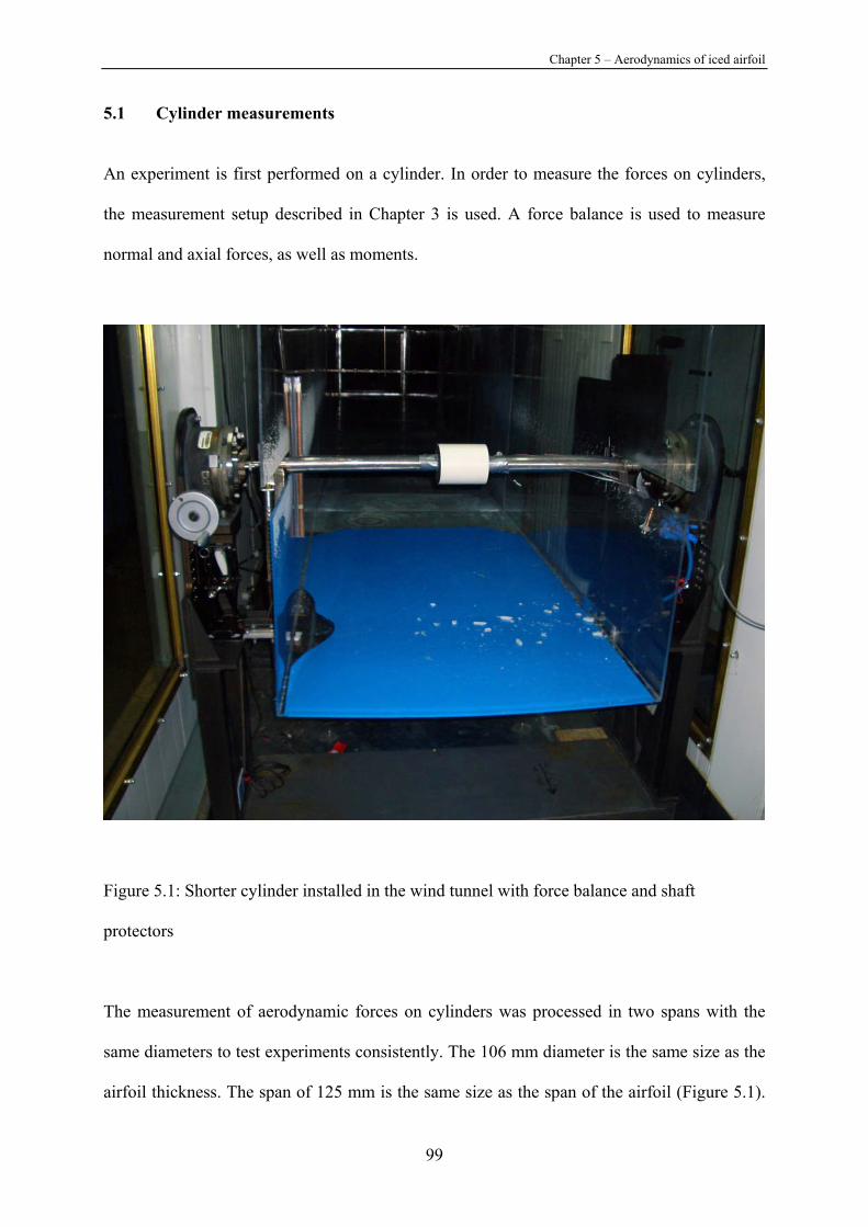
Chapter 5 – Aerodynamics of iced airfoil
99
5.1 Cylinder measurements
An experiment is first performed on a cylinder. In order to measure the forces on cylinders,
the measurement setup described in Chapter 3 is used. A force balance is used to measure
normal and axial forces, as well as moments.
Figure 5.1: Shorter cylinder installed in the wind tunnel with force balance and shaft
protectors
The measurement of aerodynamic forces on cylinders was processed in two spans with the
same diameters to test experiments consistently. The 106 mm diameter is the same size as the
airfoil thickness. The span of 125 mm is the same size as the span of the airfoil (Figure 5.1).
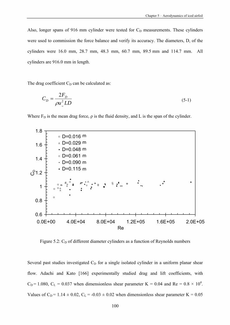
Chapter 5 – Aerodynamics of iced airfoil
100
Also, longer spans of 916 mm cylinder were tested for CD measurements. These cylinders
were used to commission the force balance and verify its accuracy. The diameters, D, of the
cylinders were 16.0 mm, 28.7 mm, 48.3 mm, 60.7 mm, 89.5 mm and 114.7 mm. All
cylinders are 916.0 mm in length.
The drag coefficient CD can be calculated as:
LDuF
C DD 2
2
∞
=ρ (5-1)
Where FD is the mean drag force, ρ is the fluid density, and L is the span of the cylinder.
0.6
0.8
1
1.2
1.4
1.6
1.8
0.0E+00 4.0E+04 8.0E+04 1.2E+05 1.6E+05 2.0E+05Re
CD
D=0.016 D=0.029D=0.048 D=0.061D=0.090D=0.115
Figure 5.2: CD of different diameter cylinders as a function of Reynolds numbers
Several past studies investigated CD for a single isolated cylinder in a uniform planar shear
flow. Adachi and Kato [166] experimentally studied drag and lift coefficients, with
CD = 1.080, CL = 0.037 when dimensionless shear parameter K = 0.04 and Re = 0.8 × 10⁴.
Values of CD = 1.14 ± 0.02, CL = -0.03 ± 0.02 when dimensionless shear parameter K = 0.05
mmmmmm
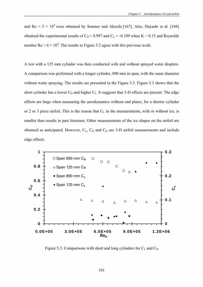
Chapter 5 – Aerodynamics of iced airfoil
101
and Re = 5 × 10⁴ were obtained by Sumner and Akosile [167]. Also, Hayashi et al. [168]
obtained the experimental results of CD = 0.997 and CL = -0.109 when K = 0.15 and Reynolds
number Re = 6 × 10⁴. The results in Figure 5.2 agree with this previous work.
A test with a 125 mm cylinder was then conducted with and without sprayed water droplets.
A comparison was performed with a longer cylinder, 890 mm in span, with the same diameter
without water spraying. The results are presented in the Figure 5.3. Figure 5.3 shows that the
short cylinder has a lower CD and higher CL. It suggests that 3-D effects are present. The edge
effects are large when measuring the aerodynamics without end plates, for a shorter cylinder
or 2 or 3 piece airfoil. This is the reason that CL in the measurements, with or without ice, is
smaller than results in past literature. Other measurements of the ice shapes on the airfoil are
obtained as anticipated. However, CL, CD and Cm are 3-D airfoil measurements and include
edge effects.
0
0.2
0.4
0.6
0.8
1
0.0E+00 3.0E+05 6.0E+05 9.0E+05 1.2E+06ReD
CD
0
0.1
0.2
0.3
CL
Span 890 mm C
Span 125 mm C
Span 890 mm C
Span 125 mm C
D
D
L
L
Figure 5.3: Comparisons with short and long cylinders for CL and CD
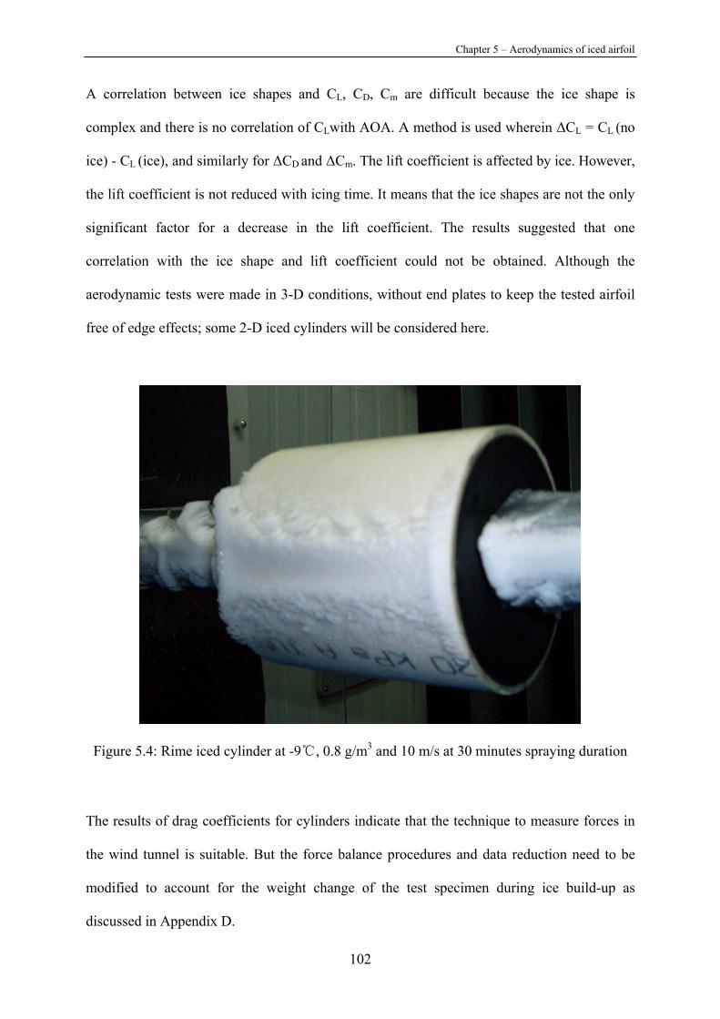
Chapter 5 – Aerodynamics of iced airfoil
102
A correlation between ice shapes and CL, CD, Cm are difficult because the ice shape is
complex and there is no correlation of CLwith AOA. A method is used wherein ∆CL = CL (no
ice) - CL (ice), and similarly for ∆CD and ∆Cm. The lift coefficient is affected by ice. However,
the lift coefficient is not reduced with icing time. It means that the ice shapes are not the only
significant factor for a decrease in the lift coefficient. The results suggested that one
correlation with the ice shape and lift coefficient could not be obtained. Although the
aerodynamic tests were made in 3-D conditions, without end plates to keep the tested airfoil
free of edge effects; some 2-D iced cylinders will be considered here.
Figure 5.4: Rime iced cylinder at -9, 0.8 g/m3 and 10 m/s at 30 minutes spraying duration
The results of drag coefficients for cylinders indicate that the technique to measure forces in
the wind tunnel is suitable. But the force balance procedures and data reduction need to be
modified to account for the weight change of the test specimen during ice build-up as
discussed in Appendix D.
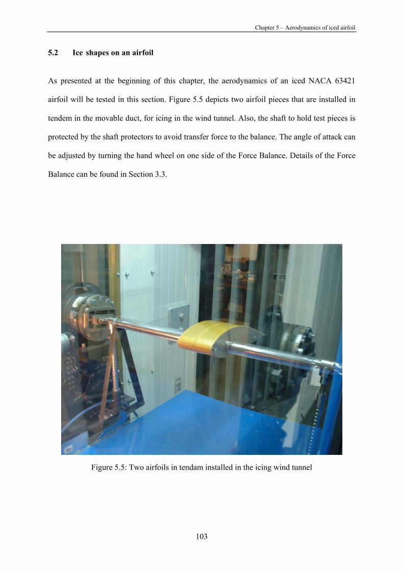
Chapter 5 – Aerodynamics of iced airfoil
103
5.2 Ice shapes on an airfoil
As presented at the beginning of this chapter, the aerodynamics of an iced NACA 63421
airfoil will be tested in this section. Figure 5.5 depicts two airfoil pieces that are installed in
tendem in the movable duct, for icing in the wind tunnel. Also, the shaft to hold test pieces is
protected by the shaft protectors to avoid transfer force to the balance. The angle of attack can
be adjusted by turning the hand wheel on one side of the Force Balance. Details of the Force
Balance can be found in Section 3.3.
Figure 5.5: Two airfoils in tendam installed in the icing wind tunnel
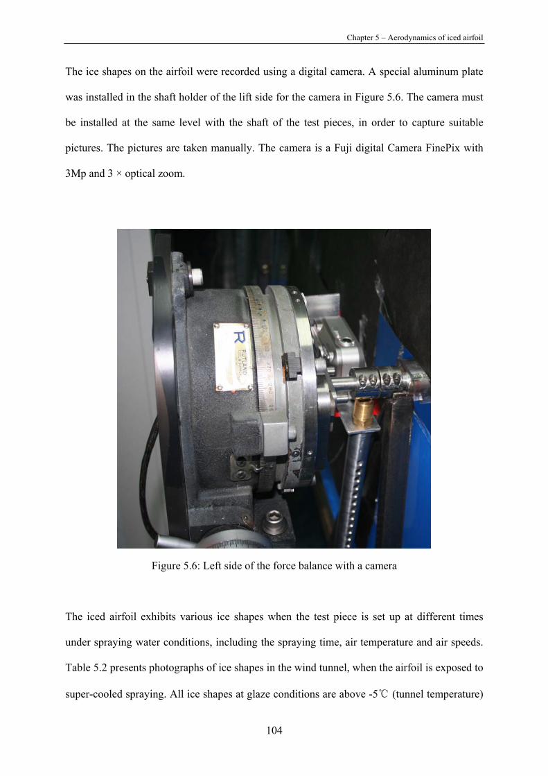
Chapter 5 – Aerodynamics of iced airfoil
104
The ice shapes on the airfoil were recorded using a digital camera. A special aluminum plate
was installed in the shaft holder of the lift side for the camera in Figure 5.6. The camera must
be installed at the same level with the shaft of the test pieces, in order to capture suitable
pictures. The pictures are taken manually. The camera is a Fuji digital Camera FinePix with
3Mp and 3 × optical zoom.
Figure 5.6: Left side of the force balance with a camera
The iced airfoil exhibits various ice shapes when the test piece is set up at different times
under spraying water conditions, including the spraying time, air temperature and air speeds.
Table 5.2 presents photographs of ice shapes in the wind tunnel, when the airfoil is exposed to
super-cooled spraying. All ice shapes at glaze conditions are above -5 (tunnel temperature)

Chapter 5 – Aerodynamics of iced airfoil
105
with a water temperature of 0. It was observed that the ice becomes thicker and thicker as
time advances. Table 5.3 shows how AOA affects the ice shapes.
Figure 5.7: Photograph of an iced airfoil at -9, 10 m/s and 0.8 g/m3
Figure 5.7 shows an original photograph of an iced airfoil at a -9 tunnel temperature with a
10 m/s wind speed and during 15 minutes spaying time at 0.8 g/m3 LWC when AOA = 9°.
The black paper is used to obtain clear ice shapes accreted on the airfoil. The side behind the
black paper is another window that can be use to put camera for photos. It is a challenge to
capture ice shapes over the airfoils. Original photos were processed using MATLAB software,
in order to obtain ice shapes. The glaze ice shapes over the airfoil are smooth and became
longer along the lower surface, when AOA increases. The reason is a stagnation point that is
different than AOA = 0. The stagnation point moves to the lower surface as AOA increases.
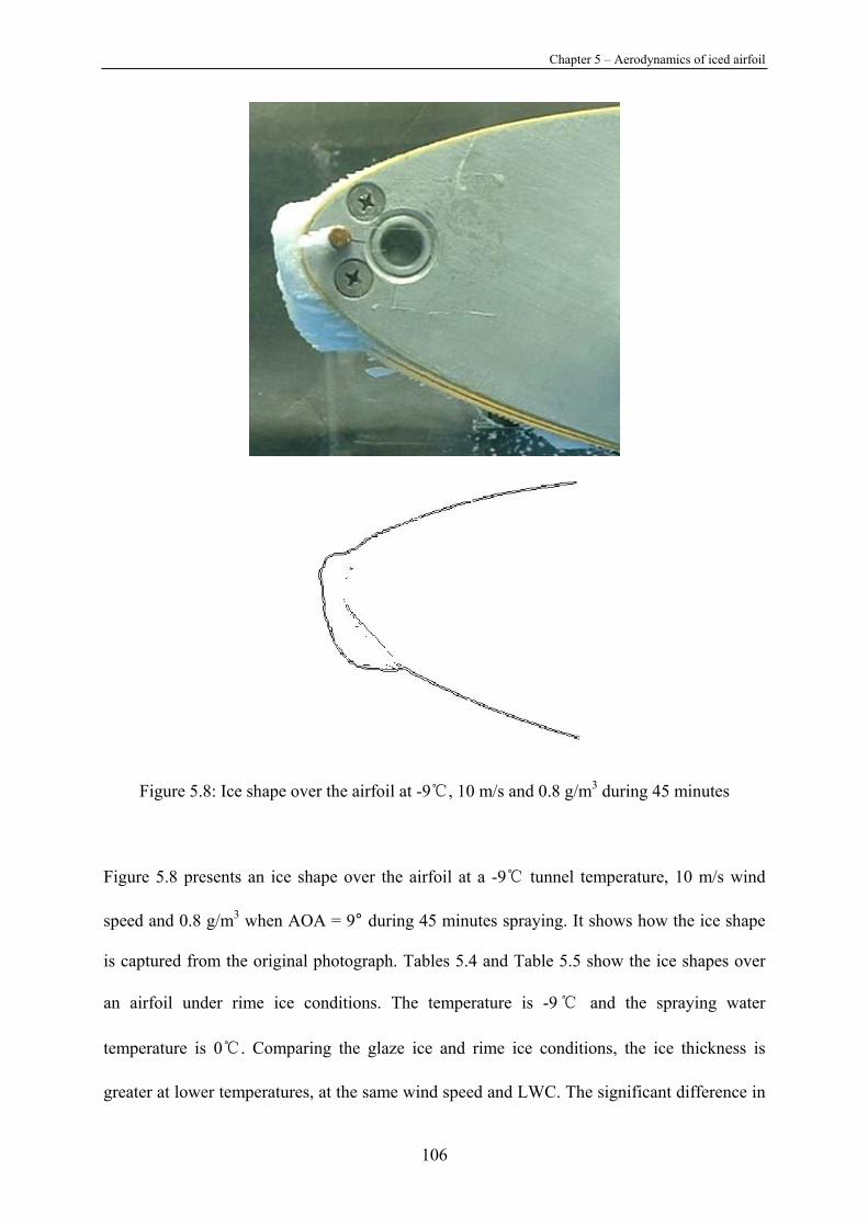
Chapter 5 – Aerodynamics of iced airfoil
106
Figure 5.8: Ice shape over the airfoil at -9, 10 m/s and 0.8 g/m3 during 45 minutes
Figure 5.8 presents an ice shape over the airfoil at a -9 tunnel temperature, 10 m/s wind
speed and 0.8 g/m3 when AOA = 9° during 45 minutes spraying. It shows how the ice shape
is captured from the original photograph. Tables 5.4 and Table 5.5 show the ice shapes over
an airfoil under rime ice conditions. The temperature is -9 and the spraying water
temperature is 0. Comparing the glaze ice and rime ice conditions, the ice thickness is
greater at lower temperatures, at the same wind speed and LWC. The significant difference in
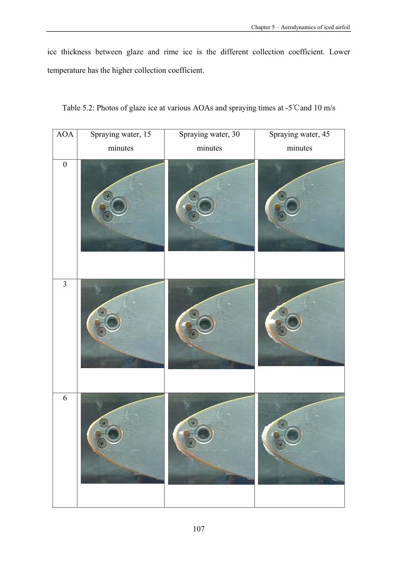
Chapter 5 – Aerodynamics of iced airfoil
107
ice thickness between glaze and rime ice is the different collection coefficient. Lower
temperature has the higher collection coefficient.
Table 5.2: Photos of glaze ice at various AOAs and spraying times at -5and 10 m/s
AOA Spraying water, 15
minutes
Spraying water, 30
minutes
Spraying water, 45
minutes
0
3
6
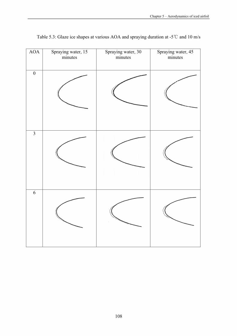
Chapter 5 – Aerodynamics of iced airfoil
108
Table 5.3: Glaze ice shapes at various AOA and spraying duration at -5 and 10 m/s
AOA Spraying water, 15 minutes
Spraying water, 30 minutes
Spraying water, 45 minutes
0
3
6
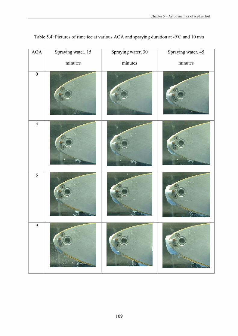
Chapter 5 – Aerodynamics of iced airfoil
109
Table 5.4: Pictures of rime ice at various AOA and spraying duration at -9 and 10 m/s
AOA Spraying water, 15
minutes
Spraying water, 30
minutes
Spraying water, 45
minutes
0
3
6
9
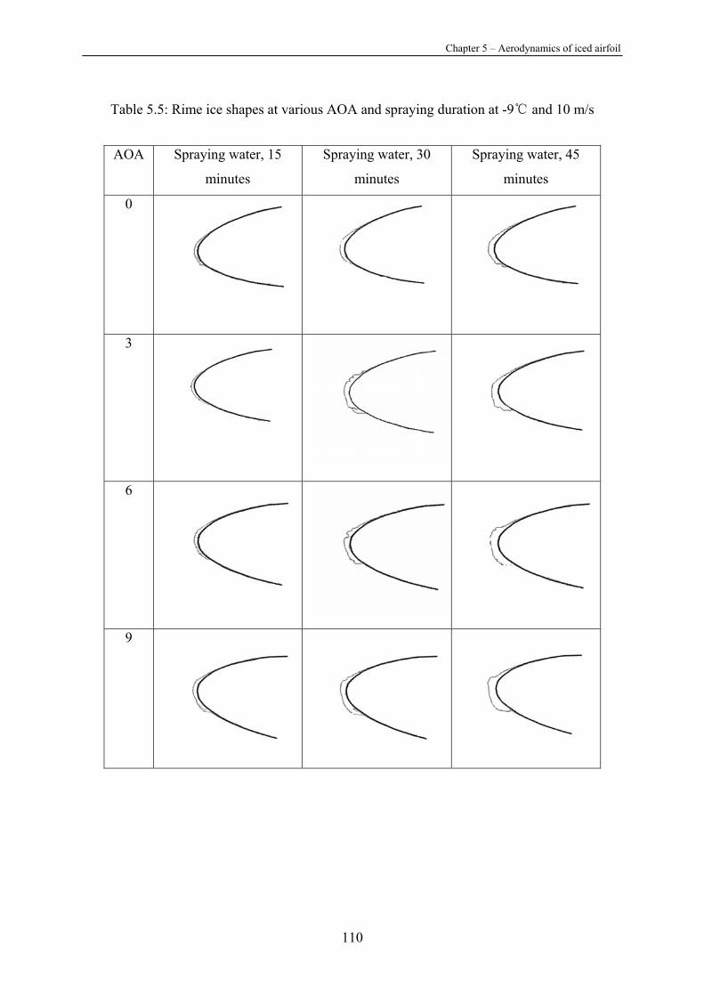
Chapter 5 – Aerodynamics of iced airfoil
110
Table 5.5: Rime ice shapes at various AOA and spraying duration at -9 and 10 m/s
AOA Spraying water, 15
minutes
Spraying water, 30
minutes
Spraying water, 45
minutes
0
3
6
9

Chapter 5 – Aerodynamics of iced airfoil
111
5.3 Aerodynamics of the iced airfoil
The last section presented the observations of ice thickness on a NACA 63421 airfoil under
glaze and rime ice conditions. The ice thickness increases with icing time. Ice changes the
airfoil profile resulting in different aerodynamics. This section will illustrate some
experimental results regarding aerodynamic characteristics of the iced airfoil.
Table 5.6 shows results when airfoils are exposed to spray at an air temperature of -5ºC for
various spraying durations and AOAs, ranging from 0º to 9º. The Reynolds number varies
from 8.3 ×10⁵ to 1.2 × 10⁶. It can be observed that CL was significantly affected by the ice.
The maximum change in CL is a drop of 96% of the uniced value when Re = 8.3 × 10⁵ (AOA
= 0) when spraying water for 30 minutes. The Reynolds number affects the lift coefficient.
The lift coefficient decreases more at low than at high Reynolds numbers. This is different
than the results at high Reynolds number, reported by Addy et al. [81]. They found that at a
Reynolds number greater than 3 × 10⁶, changes in the Reynolds number did not significantly
affect the iced airfoil performance coefficients. Also, previous research on iced airfoils shows
that the aerodynamics of an iced airfoil is relatively insensitive to variations of Re ([169,
170]). Figure 5.9 suggests that the aerodynamic conefficients of an iced airfoil are not a
strong function of Reynolds number between 8.3 × 10⁵ and 1.2 × 10⁶. When the Reynolds
number is low, ∆CL of an iced airfoil is greater than at high Reynolds numbers for the same
spraying duraton. For CD, at a low Reynolds number, the maximum increase is 55% at
AOA=6º, while spraying durations of 30 minutes.
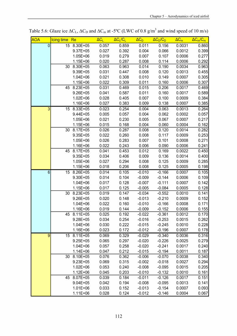
Chapter 5 – Aerodynamics of iced airfoil
112
Table 5.6: Glaze ice ∆CL, ∆CD and ∆Cm at -5ºC (LWC of 0.8 g/m3 and wind speed of 10 m/s)
AOA Icing time Re ∆CL ∆CL/CL ∆CD ∆CD/CD ∆Cm ∆Cm/Cm
0 15 8.30E+05 0.057 0.859 0.011 0.156 0.0031 0.8609.37E+05 0.027 0.392 0.004 0.066 0.0012 0.3991.05E+06 0.019 0.279 0.007 0.107 0.0006 0.2771.15E+06 0.020 0.287 0.008 0.114 0.0006 0.292
30 8.30E+05 0.063 0.963 0.014 0.190 0.0034 0.9639.39E+05 0.031 0.447 0.008 0.120 0.0013 0.4551.04E+06 0.021 0.308 0.010 0.149 0.0007 0.3051.15E+06 0.022 0.309 0.011 0.160 0.0006 0.307
45 8.23E+05 0.031 0.469 0.015 0.206 0.0017 0.4699.26E+05 0.041 0.587 0.011 0.160 0.0017 0.5891.02E+06 0.028 0.405 0.007 0.100 0.0009 0.3841.16E+06 0.027 0.383 0.009 0.138 0.0007 0.385
3 15 8.33E+05 0.023 0.254 0.004 0.063 0.0013 0.2649.44E+05 0.005 0.057 0.004 0.062 0.0002 0.0571.05E+06 0.021 0.230 0.005 0.067 0.0007 0.2171.15E+06 0.015 0.168 0.004 0.060 0.0004 0.162
30 8.17E+05 0.026 0.287 0.008 0.120 0.0014 0.2829.35E+05 0.022 0.260 0.008 0.117 0.0009 0.2531.05E+06 0.026 0.283 0.007 0.101 0.0008 0.2711.16E+06 0.022 0.243 0.006 0.090 0.0006 0.241
45 8.17E+05 0.041 0.453 0.012 0.169 0.0022 0.4509.35E+05 0.034 0.406 0.009 0.136 0.0014 0.4001.05E+06 0.027 0.294 0.008 0.125 0.0009 0.2851.15E+06 0.018 0.206 0.008 0.125 0.0005 0.198
6 15 8.26E+05 0.014 0.105 -0.010 -0.166 0.0007 0.1059.30E+05 0.014 0.104 -0.009 -0.144 0.0006 0.1091.04E+06 0.017 0.128 -0.007 -0.111 0.0007 0.1421.15E+06 0.017 0.125 -0.005 -0.084 0.0005 0.128
30 8.23E+05 0.019 0.147 -0.034 -0.552 0.0010 0.1419.26E+05 0.020 0.148 -0.013 -0.210 0.0009 0.1521.04E+06 0.022 0.160 -0.010 -0.166 0.0008 0.1711.16E+06 0.019 0.144 -0.009 -0.152 0.0006 0.155
45 8.11E+05 0.025 0.192 -0.022 -0.361 0.0012 0.1709.28E+05 0.034 0.254 -0.016 -0.253 0.0015 0.2621.04E+06 0.030 0.222 -0.015 -0.245 0.0010 0.2281.16E+06 0.023 0.172 -0.012 -0.196 0.0007 0.178
9 15 8.11E+05 0.069 0.329 -0.029 -0.340 0.0036 0.3169.25E+05 0.065 0.297 -0.020 -0.226 0.0025 0.2791.04E+06 0.057 0.258 -0.020 -0.241 0.0017 0.2401.14E+06 0.047 0.212 -0.015 -0.194 0.0011 0.187
30 8.10E+05 0.076 0.362 -0.006 -0.070 0.0038 0.3409.23E+05 0.069 0.315 -0.002 -0.018 0.0027 0.2941.02E+06 0.053 0.240 -0.008 -0.095 0.0015 0.2051.12E+06 0.045 0.203 -0.010 -0.132 0.0010 0.161
45 8.07E+05 0.039 0.184 -0.011 -0.126 0.0017 0.1519.04E+05 0.042 0.194 -0.008 -0.095 0.0013 0.1411.01E+06 0.033 0.152 -0.013 -0.154 0.0007 0.0931.11E+06 0.028 0.124 -0.012 -0.146 0.0004 0.067
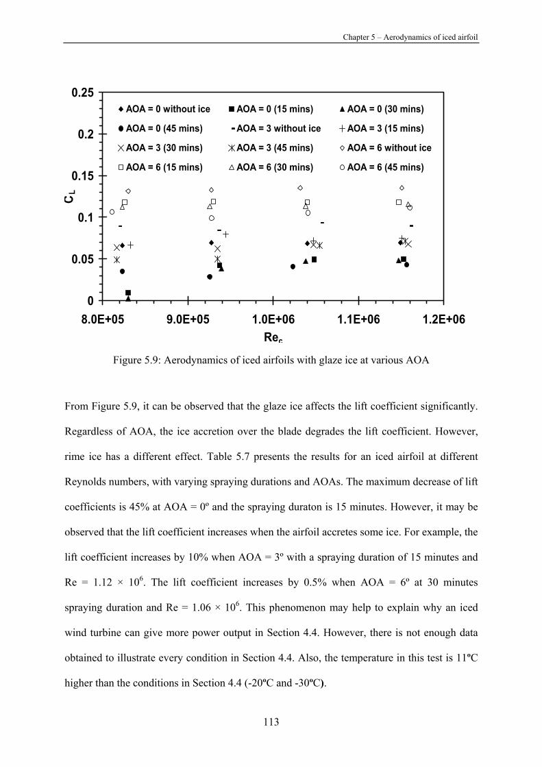
Chapter 5 – Aerodynamics of iced airfoil
113
0
0.05
0.1
0.15
0.2
0.25
8.0E+05 9.0E+05 1.0E+06 1.1E+06 1.2E+06Rec
CL
AOA = 0 without ice AOA = 0 (15 mins) AOA = 0 (30 mins)
AOA = 0 (45 mins) AOA = 3 without ice AOA = 3 (15 mins)
AOA = 3 (30 mins) AOA = 3 (45 mins) AOA = 6 without ice
AOA = 6 (15 mins) AOA = 6 (30 mins) AOA = 6 (45 mins)
Figure 5.9: Aerodynamics of iced airfoils with glaze ice at various AOA
From Figure 5.9, it can be observed that the glaze ice affects the lift coefficient significantly.
Regardless of AOA, the ice accretion over the blade degrades the lift coefficient. However,
rime ice has a different effect. Table 5.7 presents the results for an iced airfoil at different
Reynolds numbers, with varying spraying durations and AOAs. The maximum decrease of lift
coefficients is 45% at AOA = 0º and the spraying duraton is 15 minutes. However, it may be
observed that the lift coefficient increases when the airfoil accretes some ice. For example, the
lift coefficient increases by 10% when AOA = 3º with a spraying duration of 15 minutes and
Re = 1.12 × 10⁶. The lift coefficient increases by 0.5% when AOA = 6º at 30 minutes
spraying duration and Re = 1.06 × 10⁶. This phenomenon may help to explain why an iced
wind turbine can give more power output in Section 4.4. However, there is not enough data
obtained to illustrate every condition in Section 4.4. Also, the temperature in this test is 11ºC
higher than the conditions in Section 4.4 (-20ºC and -30ºC).

Chapter 5 – Aerodynamics of iced airfoil
114
Table 5.7: Rime ice aerodynamics of the iced airfoil at tunnel temperature -9ºC
(LWC 0.8 g/m3 and wind speed 10 m/s)
AOA Icing time Re ∆CL ∆CL/CL ∆CD ∆CD/CD ∆Cm ∆Cm/Cm
0 15 8.41E+05 0.038 0.458 -0.034 -0.644 0.0022 0.4769.48E+05 0.019 0.227 -0.027 -0.539 0.0010 0.2551.05E+06 0.029 0.342 -0.023 -0.475 0.0011 0.3631.17E+06 0.039 0.430 -0.016 -0.310 0.0012 0.458
30 8.16E+05 0.022 0.259 -0.031 -0.595 0.0013 0.2699.15E+05 0.017 0.204 -0.027 -0.535 0.0008 0.2091.02E+06 0.010 0.123 -0.025 -0.517 0.0004 0.1341.12E+06 0.031 0.343 -0.019 -0.372 0.0009 0.346
45 8.27E+05 0.016 0.192 -0.024 -0.461 0.0010 0.2089.36E+05 0.024 0.277 -0.029 -0.572 0.0011 0.2921.05E+06 0.020 0.239 -0.026 -0.540 0.0008 0.2551.17E+06 0.020 0.224 -0.019 -0.378 0.0006 0.242
3 15 8.15E+05 0.001 0.008 -0.027 -0.460 -0.0002 -0.0409.19E+05 0.002 0.017 -0.022 -0.382 -0.0002 -0.0471.03E+06 -0.007 -0.076 -0.018 -0.302 -0.0004 -0.1351.13E+06 -0.010 -0.102 -0.013 -0.221 -0.0004 -0.164
30 8.19E+05 0.004 0.046 -0.039 -0.662 0.0000 0.0009.33E+05 0.018 0.191 -0.033 -0.564 0.0006 0.1481.05E+06 0.020 0.206 -0.022 -0.379 0.0005 0.1691.15E+06 0.020 0.209 -0.016 -0.279 0.0005 0.173
45 8.38E+05 0.018 0.190 -0.016 -0.267 0.0010 0.1909.51E+05 0.008 0.083 -0.016 -0.269 0.0003 0.0691.07E+06 -0.092 -0.964 -0.014 -0.238 0.0001 0.0361.18E+06 0.007 0.073 -0.011 -0.191 0.0002 0.076
6 15 8.41E+05 0.012 0.087 -0.013 -0.197 0.0007 0.0989.46E+05 0.011 0.079 -0.011 -0.166 0.0004 0.0701.06E+06 0.004 0.033 -0.008 -0.120 0.0001 0.0291.17E+06 0.007 0.053 -0.005 -0.081 0.0002 0.046
30 8.34E+05 0.005 0.040 -0.019 -0.292 0.0002 0.0279.43E+05 0.001 0.007 -0.016 -0.237 0.0000 -0.0081.06E+06 -0.001 -0.005 -0.013 -0.192 0.0000 -0.0051.17E+06 0.000 0.000 -0.010 -0.156 0.0000 -0.007
45 8.41E+05 0.025 0.184 -0.016 -0.253 0.0013 0.1799.51E+05 0.020 0.147 -0.013 -0.197 0.0009 0.1471.06E+06 0.015 0.109 -0.010 -0.147 0.0005 0.1051.18E+06 0.023 0.163 -0.007 -0.098 0.0006 0.168
9 15 8.37E+05 0.009 0.043 0.008 0.081 0.0001 0.0129.53E+05 0.010 0.047 0.011 0.111 0.0003 0.0371.07E+06 0.006 0.028 0.009 0.097 0.0001 0.0091.17E+06 0.008 0.041 0.010 0.107 0.0001 0.019
30 8.37E+05 0.017 0.083 0.010 0.106 0.0006 0.0539.58E+05 0.020 0.100 0.013 0.137 0.0008 0.1001.07E+06 0.010 0.049 0.008 0.091 0.0002 0.0301.18E+06 0.015 0.072 0.010 0.112 0.0003 0.059
45 8.42E+05 0.044 0.220 -0.006 -0.066 0.0021 0.2059.58E+05 0.042 0.204 0.000 0.005 0.0017 0.2041.07E+06 0.029 0.144 0.000 0.000 0.0008 0.1271.18E+06 0.030 0.146 0.000 0.002 0.0007 0.135
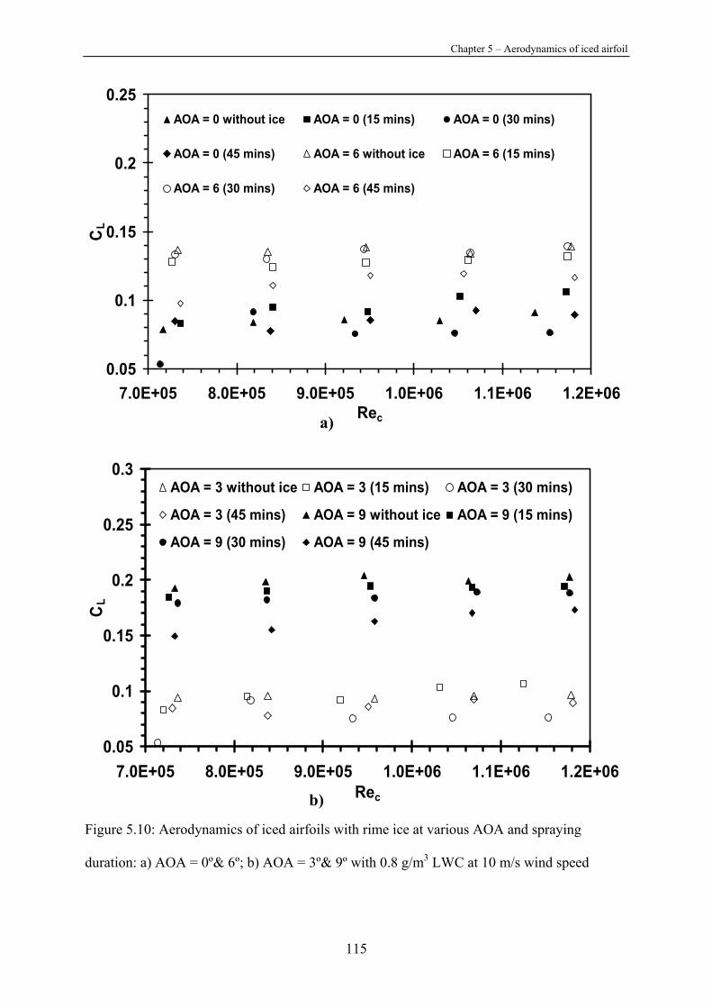
Chapter 5 – Aerodynamics of iced airfoil
115
0.05
0.1
0.15
0.2
0.25
7.0E+05 8.0E+05 9.0E+05 1.0E+06 1.1E+06 1.2E+06Rec
CL
AOA = 0 without ice AOA = 0 (15 mins) AOA = 0 (30 mins)
AOA = 0 (45 mins) AOA = 6 without ice AOA = 6 (15 mins)
AOA = 6 (30 mins) AOA = 6 (45 mins)
0.05
0.1
0.15
0.2
0.25
0.3
7.0E+05 8.0E+05 9.0E+05 1.0E+06 1.1E+06 1.2E+06Rec
CL
AOA = 3 without ice AOA = 3 (15 mins) AOA = 3 (30 mins)
AOA = 3 (45 mins) AOA = 9 without ice AOA = 9 (15 mins)
AOA = 9 (30 mins) AOA = 9 (45 mins)
Figure 5.10: Aerodynamics of iced airfoils with rime ice at various AOA and spraying
duration: a) AOA = 0º& 6º; b) AOA = 3º& 9º with 0.8 g/m3 LWC at 10 m/s wind speed
a)
b)

Chapter 5 – Aerodynamics of iced airfoil
116
Figure 5.10 illustrates the aerodynamics of a rimed airfoil at varying AOA from 0° to 9°. As
ice thicknesses increases, the lift coefficient drops. As AOA increases, the lift coefficient
drops less than AOA = 0.
The rime ice drag coefficient also can be found in Table 5.7. The maximum increase oin the
drag coefficient is 66% at Rec = 8.18 ×10⁵, AOA = 3º and a spraying duration of 30 minutes.
The increase in drag coefficient is higher at smaller AOA. Normally, as AOA varying from 0°
to 9°, the changes in drag coefficient decrease from high to low.
Chapter 5 – Aerodynamics of iced airfoil
117
5.4 Discussion of iced wind turbine results
Experimental results in Chapter 4 show that ice accretion changes the wind turbine blade
profiles and therefore decreases the wind turbine power output. The glaze iced wind turbine
blades are almost all covered by ice in Figure 4.5 and Figure 4.6. Ice can cover the blades
from the leading edge to the trailing edge. However, the rime iced blades are normally
covered only on the leading edge, as shown in Figure 4.10, as ice accumulates along the
leading edge under rime ice conditions because of the very low temperature of the blades
when water droplets impact on the surface. A water droplet impinges on a wind turbine blade
in the liquid state under glaze ice conditions. Before a water droplet changes to ice, it can flow
along the surface from the leading edge to the trailing edge, then release latent heat, turn to ice
and adhere to the blade. For rime ice conditions, the water droplets are super-cooled in the
wind tunnel before they collide with the blades, and then change to ice when they hit the
blades, thus there is no time for droplets to move along a blade. Thus, ice accretion is more
confined to the leading edge.
Comparing Figure 4.5 and Table 5.2, different ice shapes between the rotating wind turbine
blades and the 2-D airfoil are observed, under glaze ice conditions. The ice roughness on the
airfoil occurs along the leading edge of the airfoil. For the rotating 3-blade wind turbine, glaze
ice can adhere from the leading edge to the trailing edge of the blades, due to the shorter
chord of the blades and rotation of the 3-blade wind turbine. The centrifugal force lets water
droplets move when they impact the blades. Another reason is the varying pitch angles along
the twisted blades, used in most wind turbines. There are different ice shapes for iced rotating
blades and iced static blades under glaze ice conditions. Glaze ice conditions occur at just
below zero degrees Celsius. Worldwide climate change may lead to more drizzle and freezing

Chapter 5 – Aerodynamics of iced airfoil
118
rain storms, so glaze ice conditions during wind turbine operation would become more
common. Figure 4.10 and Table 5.5 show nearly the same ice shapes along the rotating blades
and static airfoils. The basic difference between rime ice and glaze ice is the temperature
when ice is occurring. Lower temperatures make water droplets change more readily to ice.
The ice thickness on a rotating blade is higher than a static airfoil if they have the same LWC
and spraying time, due to a higher relatively velocity when a water droplet hits a rotating
blade.
Comparison with Tables 5.3 and 5.5, the ice shapes are different under rime ice and glaze ice
conditions at the same spraying time and AOA. This can be explained by lower temperatures
that lead to a higher collection coefficient. A varying AOA can also change the ice shapes,
especially at the leading edge.
Ice modifies the profile of wind turbine blades, regardless of glaze or rime ice conditions. Iced
blades affect the power generation as measured in Chapter 5, so appropriate methods need to
be considered when turbines are operating in cold climates. Further research on coating
materials [100] provides methods for anti-icing, de-icing and ice-phobic materials. Using ice-
phobic material surface coatings is insufficient, so a heating surface provides an additional
method for anti-icing and de-icing, when wind turbines operate under icing conditions.
Results in Chapter 6 have provided heat transfer correlations of the heat transfer coefficient
for these purposes.
From Chapters 4 and 5, it was examined how ice adheres to the leading edge of a wind turbine
blade. The heat transfer correlations in Chapter 6 provide average values for the entire airfoil.
According to recommendations in Ref. [98], an entire heater over the blade surface is better

Chapter 5 – Aerodynamics of iced airfoil
119
for anti-icing and de-icing, under extreme cold conditions. These trends were observed in
experimental results in Chapter 4, for glaze ice conditions. For most drizzle and freezing rain
conditions, a heater over an entire wind turbine blade is necessary for de-icing and anti-icing.
Also, the heat transfer correlation at the leading edge (10% chord along the blades, 0.1c) is
higher than 1.7 times the average correlation. The heat transfer correlation at the leading edge
(20% chord along the blades, 0.2c) is higher than 1.4 times the average correlation. This can
be used to calculate the heat transfer correlation for a heater at the leading edge. From
Chapters 4 and 5, most ice cover lies in the range of 0.1c. According to results in Ref. [100], a
useful method is an ice-phobic material and a heater strip at the leading edge up to 0.1c, for
most blade sections in icing condition areas. The results provide a useful method to calculate
the energy required when wind turbine blades need to be installed with a heater or a built-in
heat strip.
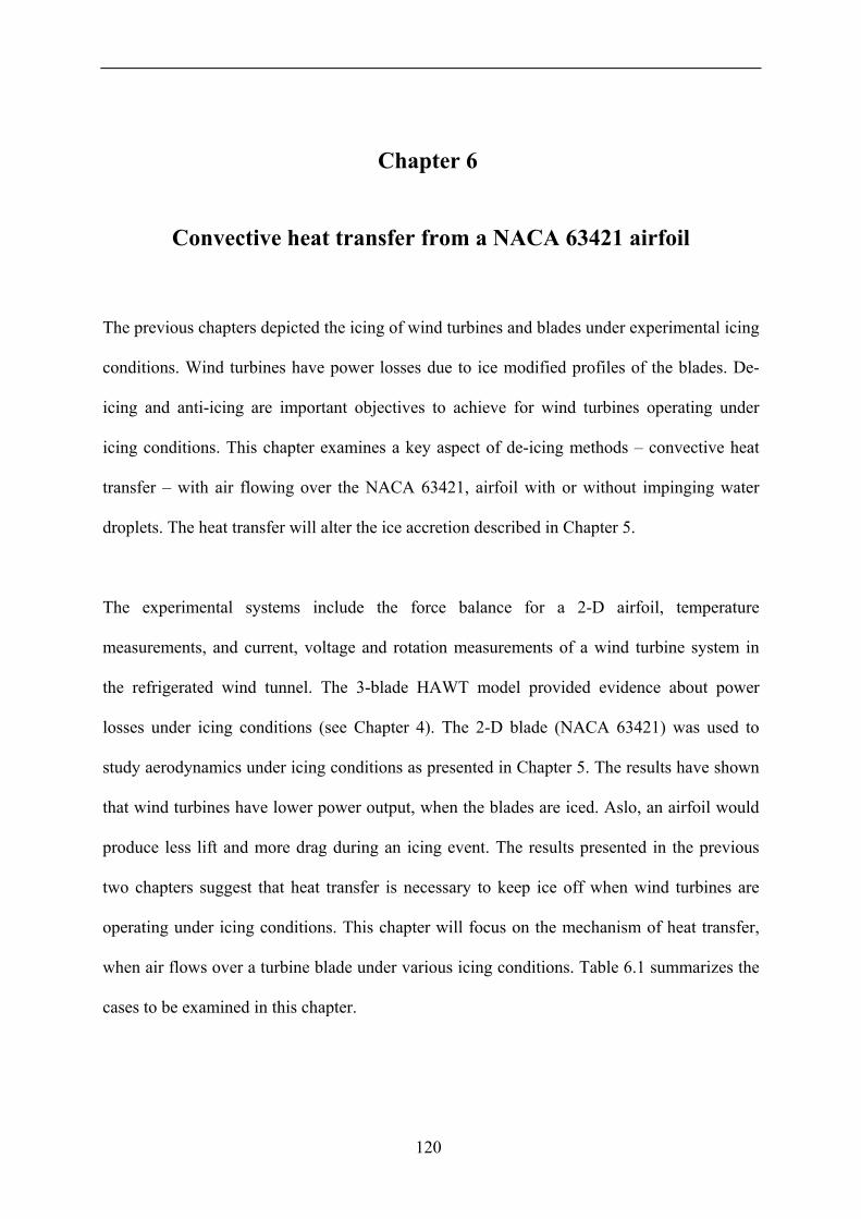
120
Chapter 6
Convective heat transfer from a NACA 63421 airfoil
The previous chapters depicted the icing of wind turbines and blades under experimental icing
conditions. Wind turbines have power losses due to ice modified profiles of the blades. De-
icing and anti-icing are important objectives to achieve for wind turbines operating under
icing conditions. This chapter examines a key aspect of de-icing methods – convective heat
transfer – with air flowing over the NACA 63421, airfoil with or without impinging water
droplets. The heat transfer will alter the ice accretion described in Chapter 5.
The experimental systems include the force balance for a 2-D airfoil, temperature
measurements, and current, voltage and rotation measurements of a wind turbine system in
the refrigerated wind tunnel. The 3-blade HAWT model provided evidence about power
losses under icing conditions (see Chapter 4). The 2-D blade (NACA 63421) was used to
study aerodynamics under icing conditions as presented in Chapter 5. The results have shown
that wind turbines have lower power output, when the blades are iced. Aslo, an airfoil would
produce less lift and more drag during an icing event. The results presented in the previous
two chapters suggest that heat transfer is necessary to keep ice off when wind turbines are
operating under icing conditions. This chapter will focus on the mechanism of heat transfer,
when air flows over a turbine blade under various icing conditions. Table 6.1 summarizes the
cases to be examined in this chapter.

Chapter 6 Convective heat transfer
121
Table 6.1: Experimental conditions during convective heat transfer
Without LWC With LWC
AOA 0° 5°, 10°, 15°, 20°, 25° 0° 5°, 10°, 15°, 20°, 25°
Temperature 10°C, 0°C, -5°C, -10°C, -15°C, -20°C,
-25°C, -30°C
3°C, 10°C
LWC 0 g/m3 0 ~ 2 g/m3
T (water) N/A 10°C
Heater 45 V, 1.3 A 50 V, 1.5 A
Wind speed 0 ~ 33 m/s 0 ~ 33 m/s
6.1 Heat transfer characterization at 0 AOA
In this section, experimental results are presented for convective heat transfer from a NACA
63421 airfoil at varying Reynolds numbers. These variations are obtained by changing the
icing tunnel air velocity and the air temperature in order to vary the air viscosity, density and
thermal diffusivity. Within the refrigerated wind tunnel (Figure 3.1), air temperatures were
varied between 20oC and -30oC. This temperature range yields Prandtl numbers in Table 6.2.
Table 6.2: The range of Prandtl numbers in the experiments
Prandtl Number Temperature 0.7098 20oC 0.7125 10oC 0.715 0oC 0.7166 -5oC 0.7181 -10oC 0.7196 -15oC 0.7211 -20oC 0.7226 -25oC
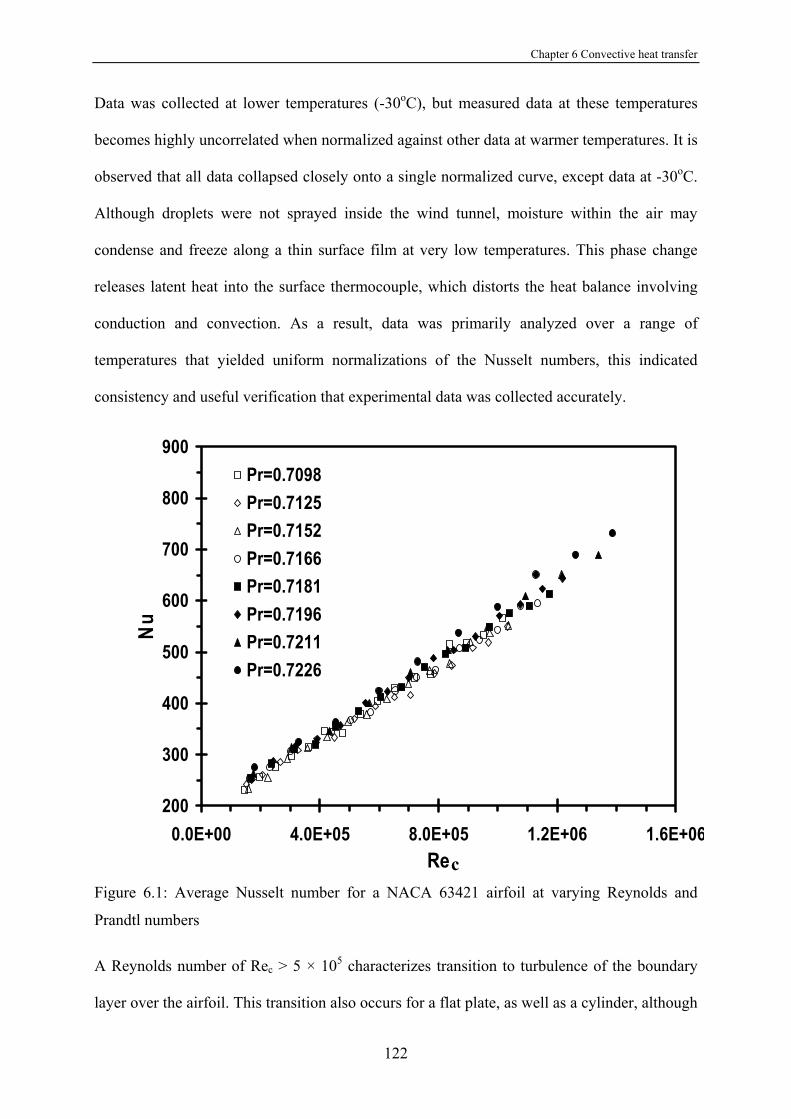
Chapter 6 Convective heat transfer
122
Data was collected at lower temperatures (-30oC), but measured data at these temperatures
becomes highly uncorrelated when normalized against other data at warmer temperatures. It is
observed that all data collapsed closely onto a single normalized curve, except data at -30oC.
Although droplets were not sprayed inside the wind tunnel, moisture within the air may
condense and freeze along a thin surface film at very low temperatures. This phase change
releases latent heat into the surface thermocouple, which distorts the heat balance involving
conduction and convection. As a result, data was primarily analyzed over a range of
temperatures that yielded uniform normalizations of the Nusselt numbers, this indicated
consistency and useful verification that experimental data was collected accurately.
200
300
400
500
600
700
800
900
0.0E+00 4.0E+05 8.0E+05 1.2E+06 1.6E+06Re
Nu
Pr=0.7098Pr=0.7125Pr=0.7152Pr=0.7166Pr=0.7181Pr=0.7196Pr=0.7211Pr=0.7226
Figure 6.1: Average Nusselt number for a NACA 63421 airfoil at varying Reynolds and
Prandtl numbers
A Reynolds number of Rec > 5 × 10⁵ characterizes transition to turbulence of the boundary
layer over the airfoil. This transition also occurs for a flat plate, as well as a cylinder, although
c
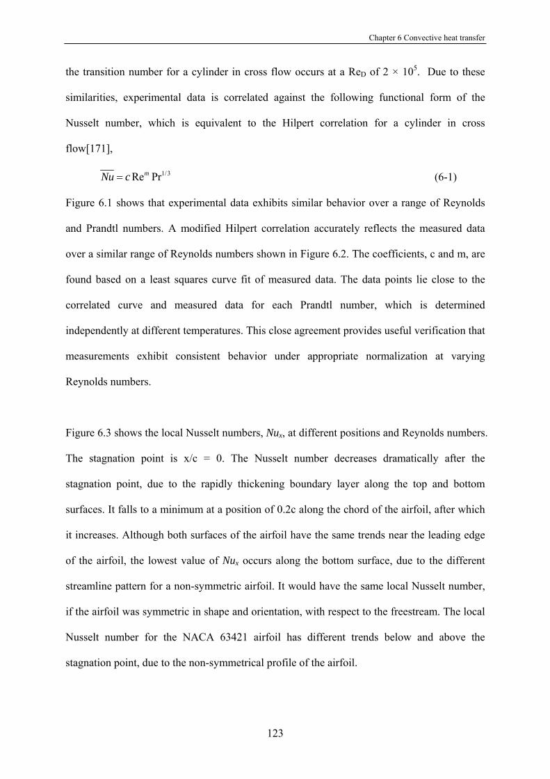
Chapter 6 Convective heat transfer
123
the transition number for a cylinder in cross flow occurs at a ReD of 2 × 10⁵. Due to these
similarities, experimental data is correlated against the following functional form of the
Nusselt number, which is equivalent to the Hilpert correlation for a cylinder in cross
flow[171],
1/3Re PrmNu c= (6-1)
Figure 6.1 shows that experimental data exhibits similar behavior over a range of Reynolds
and Prandtl numbers. A modified Hilpert correlation accurately reflects the measured data
over a similar range of Reynolds numbers shown in Figure 6.2. The coefficients, c and m, are
found based on a least squares curve fit of measured data. The data points lie close to the
correlated curve and measured data for each Prandtl number, which is determined
independently at different temperatures. This close agreement provides useful verification that
measurements exhibit consistent behavior under appropriate normalization at varying
Reynolds numbers.
Figure 6.3 shows the local Nusselt numbers, Nux, at different positions and Reynolds numbers.
The stagnation point is x/c = 0. The Nusselt number decreases dramatically after the
stagnation point, due to the rapidly thickening boundary layer along the top and bottom
surfaces. It falls to a minimum at a position of 0.2c along the chord of the airfoil, after which
it increases. Although both surfaces of the airfoil have the same trends near the leading edge
of the airfoil, the lowest value of Nux occurs along the bottom surface, due to the different
streamline pattern for a non-symmetric airfoil. It would have the same local Nusselt number,
if the airfoil was symmetric in shape and orientation, with respect to the freestream. The local
Nusselt number for the NACA 63421 airfoil has different trends below and above the
stagnation point, due to the non-symmetrical profile of the airfoil.
Chapter 6 Convective heat transfer
124
5.5
6
6.5
7
7.5
8
11.5 12 12.5 13 13.5 14 14.5Ln(Rec)
Ln( N
u/Pr
1/3 )
Pr=0.709Pr=0.712Pr=0.715Pr=0.717pr=0.718Pr=0.720Pr=0.721Pr=0.722Pr=0.721, c=0.0943, m=0.636Pr=0.718, c=0.0943, m=0.636Pr=0.718, c=2.48, m=0.389Pr=0.712, c=2.48, m=0.389
Figure 6.2: Normalized Nusselt function correlation
0
200
400
600
800
1000
1200
1400
1600
1800
2000
-0.6 -0.3 0 0.3 0.6 0.9Non-dimensional chord position
Nu x
Re=186,000 Re=330,000Re=478,868 Re=620,112Re=757,878 Re=897,117Re=1,037,270 Re=1,170,358Re=1,435,573 Re=1,304,821
Figure 6.3: Local Nusselt number at varying chord positions (x/c)

Chapter 6 Convective heat transfer
125
6.1.2 Sensitivity study for correlation coefficients
Sensitivity studies involving the effects of varying correlation coefficients, c and m, are
illustrated in Figure 6.4 (0ºC, Pr = 0.715) and Figure 6.5 (-10ºC, Pr = 0.718). The purpose of
these studies is to better understand sensitivity of the correlation to changes of the empirical
coefficients. In Figure 6.4a, the central line represents c = 2.483 and m = 0.389. The following
correlation of Nu closely agrees with the experimental data,
0.389 1/32.483Re PrNu = (for Re ≤ 5 × 10⁵) (6-2)
In Figure 6.4a, the m-coefficient is kept constant, while the c-coefficient varies over a range
of values to show sensitivity of the correlation with respect to the c-coefficient. In contrast,
Figure 6.4b shows sensitivity with respect to the m-coefficient, while the c-coefficient is kept
constant. Unlike Reynolds numbers below Re = 5 × 10⁵ (laminar flow regime) in Figure 6.4,
sensitivity studies at higher Reynolds numbers (turbulent flow regime) are illustrated in
Figure 6.5a and b. Similar trends are observed both in Figure 6.4 and 6.5, with respect to
sensitivity to the c-coefficient and m-coefficient. The following correlation is obtained for
turbulent flow conditions: c = 0.0943 and m = 0.636.
0.636 1/30.0943Re PrNu = (for Re > 5 × 10⁵) (6-3)
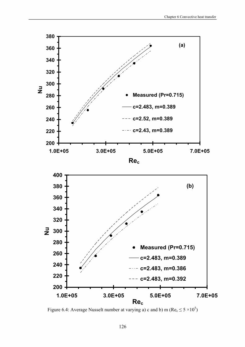
Chapter 6 Convective heat transfer
126
200
220
240
260
280
300
320
340
360
380
1.0E+05 3.0E+05 5.0E+05 7.0E+05Re
Nu
Measured (Pr=0.715)
c=2.483, m=0.389
c=2.52, m=0.389
c=2.43, m=0.389
(a)
200
220
240
260
280
300
320
340
360
380
400
1.0E+05 3.0E+05 5.0E+05 7.0E+05Re
Nu
Measured (Pr=0.715)
c=2.483, m=0.389
c=2.483, m=0.386
c=2.483, m=0.392
(b)
Figure 6.4: Average Nusselt number at varying a) c and b) m (Rec ≤ 5 ×10⁵)
Rec
Rec

Chapter 6 Convective heat transfer
127
340
390
440
490
540
590
640
4.0E+05 8.0E+05 1.2E+06 1.6E+06Re
Nu
Measured (Pr=0.718)
c=0.0943, m=0.636
c=0.0943, m=0.638
c=0.0943, m=0.634
(a)
250
300
350
400
450
500
550
600
650
700
4.0E+05 8.0E+05 1.2E+06 1.6E+06Re
Nu
Measured (Pr=0.718)
c=0.098, m=0.636
c=0.091, m=0.636
c=0.0943, m=0.636
(b)
Figure 6.5: Average Nusselt number at varying a) c and b) m (Rec > 5 ×10⁵)
Rec
Rec

Chapter 6 Convective heat transfer
128
6.1.3 Comparison with past methods
The previous study used thermocouples to measure surface temperatures, which were
subsequently used in heat balances to establish the convective heat transfer coefficients. Many
similar past studies have shown that thermocouple measurements can provide an effective
method for determining these coefficients. Sanitjai and Goldstein [172] measured both local
and average convection coefficients for a circular cylinder, with eight T-type (copper–
constantan) thermocouples installed under the heated surface. The authors studied Reynolds
numbers between 2,000 and 90,000 and Prandtl numbers between 0.7 and 176, in air, water
and six mixtures of ethylene glycol and water. In a similar way as Equations 6-2 and 6-3, the
authors separated the empirical correlations into distinct regions, namely the laminar
boundary layer, reattachment and periodic vortex flow regions. Chang and Mills [173] used an
RdF microfoil heat flux sensor with T-type thermocouples installed on the center plane of a
cylinder to measure local surface temperatures and convection coefficients for a cylinder in
cross flow. The authors presented correlations for the average Nusselt numbers, while
including effects of wind tunnel blockage and freestream turbulence on the correlations.
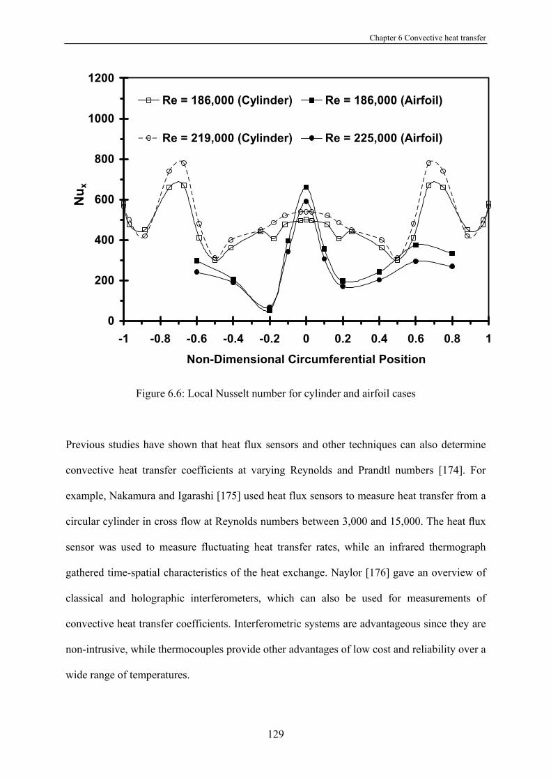
Chapter 6 Convective heat transfer
129
0
200
400
600
800
1000
1200
-1 -0.8 -0.6 -0.4 -0.2 0 0.2 0.4 0.6 0.8 1
Non-Dimensional Circumferential Position
Nu x
Re = 186,000 (Cylinder) Re = 186,000 (Airfoil)
Re = 219,000 (Cylinder) Re = 225,000 (Airfoil)
Figure 6.6: Local Nusselt number for cylinder and airfoil cases
Previous studies have shown that heat flux sensors and other techniques can also determine
convective heat transfer coefficients at varying Reynolds and Prandtl numbers [174]. For
example, Nakamura and Igarashi [175] used heat flux sensors to measure heat transfer from a
circular cylinder in cross flow at Reynolds numbers between 3,000 and 15,000. The heat flux
sensor was used to measure fluctuating heat transfer rates, while an infrared thermograph
gathered time-spatial characteristics of the heat exchange. Naylor [176] gave an overview of
classical and holographic interferometers, which can also be used for measurements of
convective heat transfer coefficients. Interferometric systems are advantageous since they are
non-intrusive, while thermocouples provide other advantages of low cost and reliability over a
wide range of temperatures.

Chapter 6 Convective heat transfer
130
The circular cylinder and flat plate are the most common geometrical configurations, which
have received most attention of past research studies. Correlations have been reported in
textbooks [171] and review articles [177].
Figure 6.6 compares the local Nusselt number for a circular cylinder with an airfoil. Two
curves at different Reynolds numbers are shown for each case. For the cylinder, it can be
observed that the local Nusselt number variation is symmetric, with respect to the upper and
lower surfaces. Also, two minimum points of the local Nusselt number are observed. This
occurs from the laminar boundary layer development after the stagnation point, followed by
boundary layer transition from laminar to turbulent flow. A second minimum of the local
Nusselt number arises on the downstream side of the cylinder. After the separation point in
the wake region, the local Nusselt number increases due to turbulent mixing in the wake.
Turbulent flow conditions occur when Re > 2 × 10⁵. Both cases in Figure 6.6 exceed this
Reynolds number.
The local Nusselt number distribution for the airfoil is significantly different than for the
circular cylinder. Only a single minimum value is observed and the maximum occurs at the
stagnation point. The boundary layer growth causes the local Nusselt number to decrease, as
the air flows over the airfoil downstream of the stagnation point. The local Nusselt number
reaches a minimum at 0.2c and Nux along the lower surface becomes smaller than values on
the uper surface. The local Nusselt number increases after 0.2c. The maximum Nusselt
number at the stagnation point (not at 0.6c) is significantly different than the cylinder.
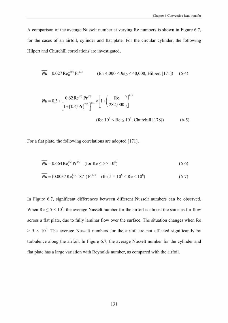
Chapter 6 Convective heat transfer
131
A comparison of the average Nusselt number at varying Re numbers is shown in Figure 6.7,
for the cases of an airfoil, cylinder and flat plate. For the circular cylinder, the following
Hilpert and Churchill correlations are investigated,
0.805 1/30.027 Re PrDNu = (for 4,000 < ReD < 40,000; Hilpert [171]) (6-4)
( )
4/51/ 2 1/3
1/ 42/3
0.62Re Pr Re0.3 1282,0001 0.4 Pr
Nu⎡ ⎤⎛ ⎞= + × +⎢ ⎥⎜ ⎟
⎝ ⎠⎡ ⎤ ⎣ ⎦+⎣ ⎦
(for 102 < Re ≤ 107; Churchill [178]) (6-5)
For a flat plate, the following correlations are adopted [171],
1/ 2 1/30.664Re PrxNu = (for Re ≤ 5 × 10⁵) (6-6)
4/5 1/3(0.0037Re 871) PrLNu = − (for 5 × 10⁵ < Re < 108) (6-7)
In Figure 6.7, significant differences between different Nusselt numbers can be observed.
When Re ≤ 5 × 10⁵, the average Nusselt number for the airfoil is almost the same as for flow
across a flat plate, due to fully laminar flow over the surface. The situation changes when Re
> 5 × 10⁵. The average Nusselt numbers for the airfoil are not affected significantly by
turbulence along the airfoil. In Figure 6.7, the average Nusselt number for the cylinder and
flat plate has a large variation with Reynolds number, as compared with the airfoil.
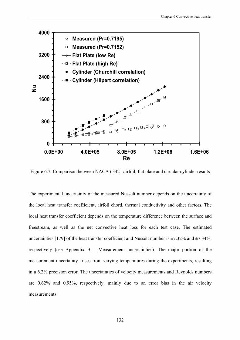
Chapter 6 Convective heat transfer
132
0
800
1600
2400
3200
4000
0.0E+00 4.0E+05 8.0E+05 1.2E+06 1.6E+06Re
Nu
Measured (Pr=0.7195)Measured (Pr=0.7152)Flat Plate (low Re)Flat Plate (high Re)Cylinder (Churchill correlation)Cylinder (Hilpert correlation)
Figure 6.7: Comparison between NACA 63421 airfoil, flat plate and circular cylinder results
The experimental uncertainty of the measured Nusselt number depends on the uncertainty of
the local heat transfer coefficient, airfoil chord, thermal conductivity and other factors. The
local heat transfer coefficient depends on the temperature difference between the surface and
freestream, as well as the net convective heat loss for each test case. The estimated
uncertainties [179] of the heat transfer coefficient and Nusselt number is ±7.32% and ±7.34%,
respectively (see Appendix B – Measurement uncertainties). The major portion of the
measurement uncertainty arises from varying temperatures during the experiments, resulting
in a 6.2% precision error. The uncertainties of velocity measurements and Reynolds numbers
are 0.62% and 0.95%, respectively, mainly due to an error bias in the air velocity
measurements.
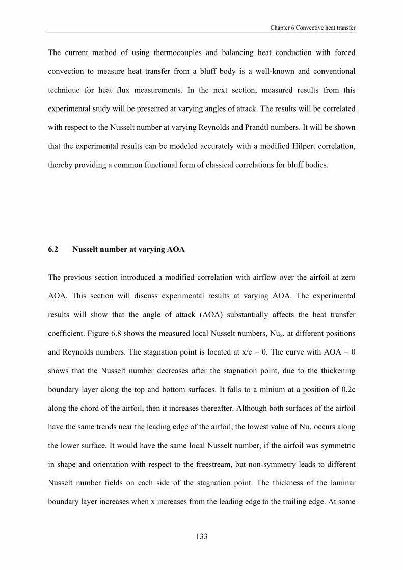
Chapter 6 Convective heat transfer
133
The current method of using thermocouples and balancing heat conduction with forced
convection to measure heat transfer from a bluff body is a well-known and conventional
technique for heat flux measurements. In the next section, measured results from this
experimental study will be presented at varying angles of attack. The results will be correlated
with respect to the Nusselt number at varying Reynolds and Prandtl numbers. It will be shown
that the experimental results can be modeled accurately with a modified Hilpert correlation,
thereby providing a common functional form of classical correlations for bluff bodies.
6.2 Nusselt number at varying AOA
The previous section introduced a modified correlation with airflow over the airfoil at zero
AOA. This section will discuss experimental results at varying AOA. The experimental
results will show that the angle of attack (AOA) substantially affects the heat transfer
coefficient. Figure 6.8 shows the measured local Nusselt numbers, Nux, at different positions
and Reynolds numbers. The stagnation point is located at x/c = 0. The curve with AOA = 0
shows that the Nusselt number decreases after the stagnation point, due to the thickening
boundary layer along the top and bottom surfaces. It falls to a minium at a position of 0.2c
along the chord of the airfoil, then it increases thereafter. Although both surfaces of the airfoil
have the same trends near the leading edge of the airfoil, the lowest value of Nux occurs along
the lower surface. It would have the same local Nusselt number, if the airfoil was symmetric
in shape and orientation with respect to the freestream, but non-symmetry leads to different
Nusselt number fields on each side of the stagnation point. The thickness of the laminar
boundary layer increases when x increases from the leading edge to the trailing edge. At some

Chapter 6 Convective heat transfer
134
points along each surface, the boundary layer transition occurs and the boundary layer
becomes turbulent. In the laminar region, the heat transfer coefficient decreases as the
thickness of the boundary layer increases. The heat transfer coefficient increases as the
boundary layer becomes turbulent.
In Figure 6.8a, it can be observed how the Nusselt number changes with AOA, for the case of
low Reynolds number (Re ≤ 5 × 10⁵). At the stagnation point, the Nusselt number remains
nearly uniform at different values of AOA. However, it can change significantly with AOA
along the chord of the airfoil. The Nusselt number decreases significantly at ±0.1c, -0.4c and
0.6c, and it increases at -0.2c, -0.6c and 0.4c. Figure 4b shows the Nusselt number results for
cases of high Reynolds numbers. At angles of attack of 5° and 10°, the local Nusselt number
at the stagnation point is lower than the case for 0°. Also, values of the Nusselt number at 0.4c
and +0.6c are lower than AOA of zero at those points. In contrast, the values of Nusselt
number at -0.1c, -0.2c and -0.6c are higher than an AOA of zero at the same points. As AOA
increases, the changes of local Nu with AOA become more pronounced at higher Reynolds
numbers. The Nusselt number at the stagnation point is higher than the value of Nu at the
stagnation point when the angle of attack is 0°. Also, only two points of the local Nu number
along the airfoil, -0.4c and +0.6c, have lower values than the Nusselt number at 0° for the
same points. Furthermore, Nux for the other points along the airfoil are larger than the value
of the local Nu number at the same points for 0°. The average Nu number is expected to have
similar distinct trends at high Reynolds numbers.
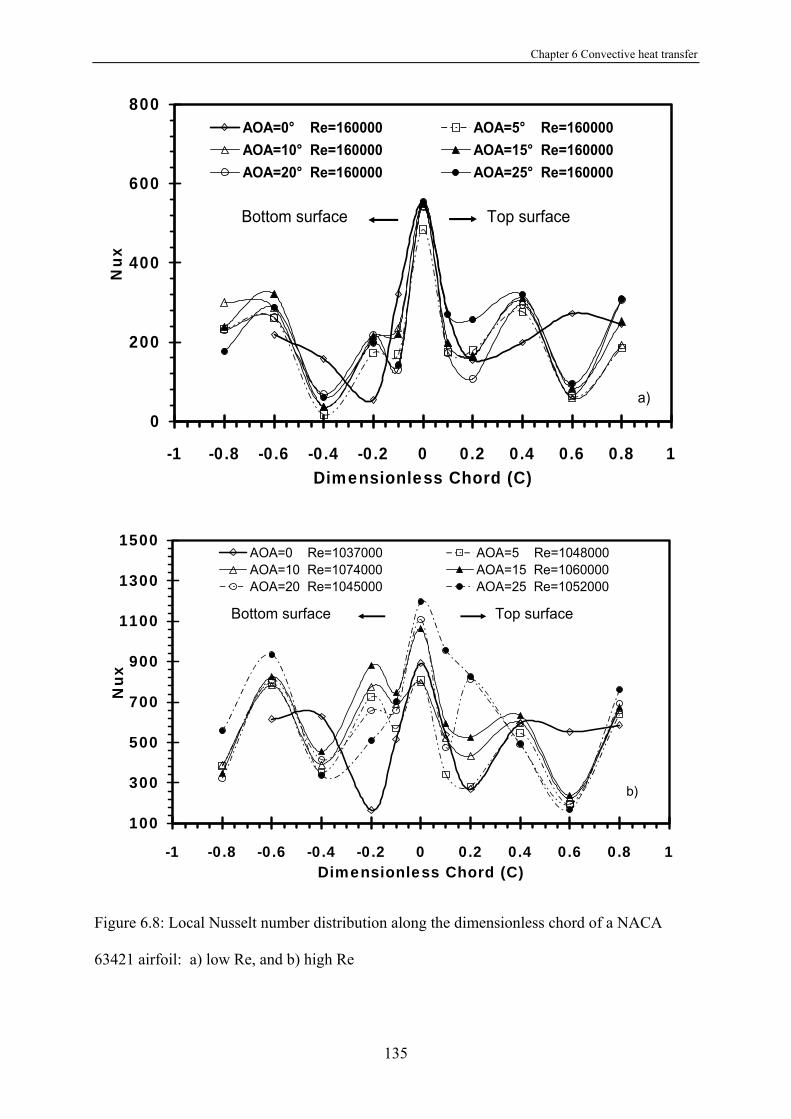
Chapter 6 Convective heat transfer
135
0
200
400
600
800
-1 -0.8 -0.6 -0.4 -0.2 0 0.2 0.4 0.6 0.8 1Dimensionless Chord (C)
Nux
AOA=0° Re=160000 AOA=5° Re=160000AOA=10° Re=160000 AOA=15° Re=160000AOA=20° Re=160000 AOA=25° Re=160000
a)
Bottom surface Top surface
100
300
500
700
900
1100
1300
1500
-1 -0.8 -0.6 -0.4 -0.2 0 0.2 0.4 0.6 0.8 1Dimensionless Chord (C)
Nux
AOA=0 Re=1037000 AOA=5 Re=1048000AOA=10 Re=1074000 AOA=15 Re=1060000AOA=20 Re=1045000 AOA=25 Re=1052000
b)
Bottom surface Top surface
Figure 6.8: Local Nusselt number distribution along the dimensionless chord of a NACA
63421 airfoil: a) low Re, and b) high Re
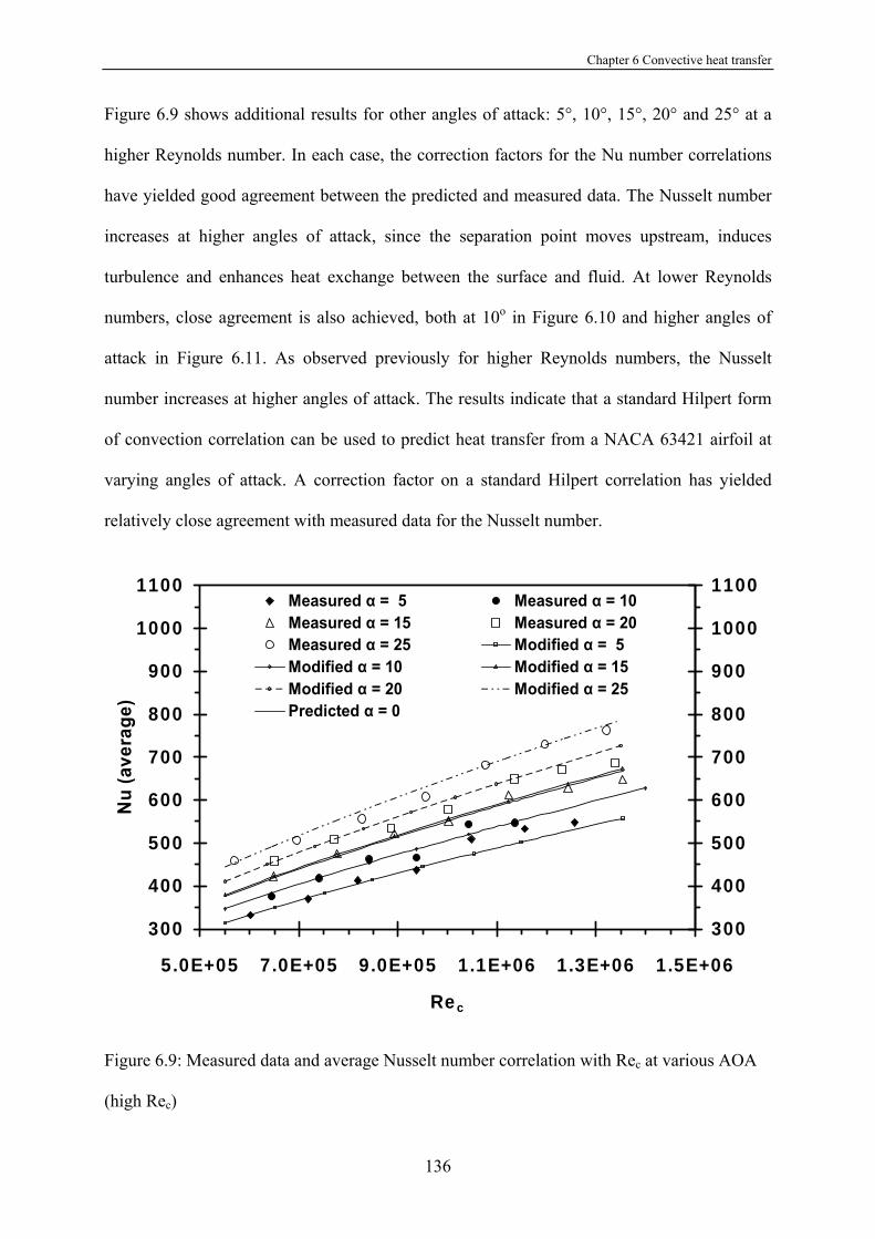
Chapter 6 Convective heat transfer
136
Figure 6.9 shows additional results for other angles of attack: 5°, 10°, 15°, 20° and 25° at a
higher Reynolds number. In each case, the correction factors for the Nu number correlations
have yielded good agreement between the predicted and measured data. The Nusselt number
increases at higher angles of attack, since the separation point moves upstream, induces
turbulence and enhances heat exchange between the surface and fluid. At lower Reynolds
numbers, close agreement is also achieved, both at 10o in Figure 6.10 and higher angles of
attack in Figure 6.11. As observed previously for higher Reynolds numbers, the Nusselt
number increases at higher angles of attack. The results indicate that a standard Hilpert form
of convection correlation can be used to predict heat transfer from a NACA 63421 airfoil at
varying angles of attack. A correction factor on a standard Hilpert correlation has yielded
relatively close agreement with measured data for the Nusselt number.
300
400
500
600
700
800
900
1000
1100
5.0E+05 7.0E+05 9.0E+05 1.1E+06 1.3E+06 1.5E+06
Rec
Nu
(ave
rage
)
300
400
500
600
700
800
900
1000
1100Measured α = 5 Measured α = 10Measured α = 15 Measured α = 20Measured α = 25 Modified α = 5Modified α = 10 Modified α = 15Modified α = 20 Modified α = 25Predicted α = 0
Figure 6.9: Measured data and average Nusselt number correlation with Rec at various AOA
(high Rec)
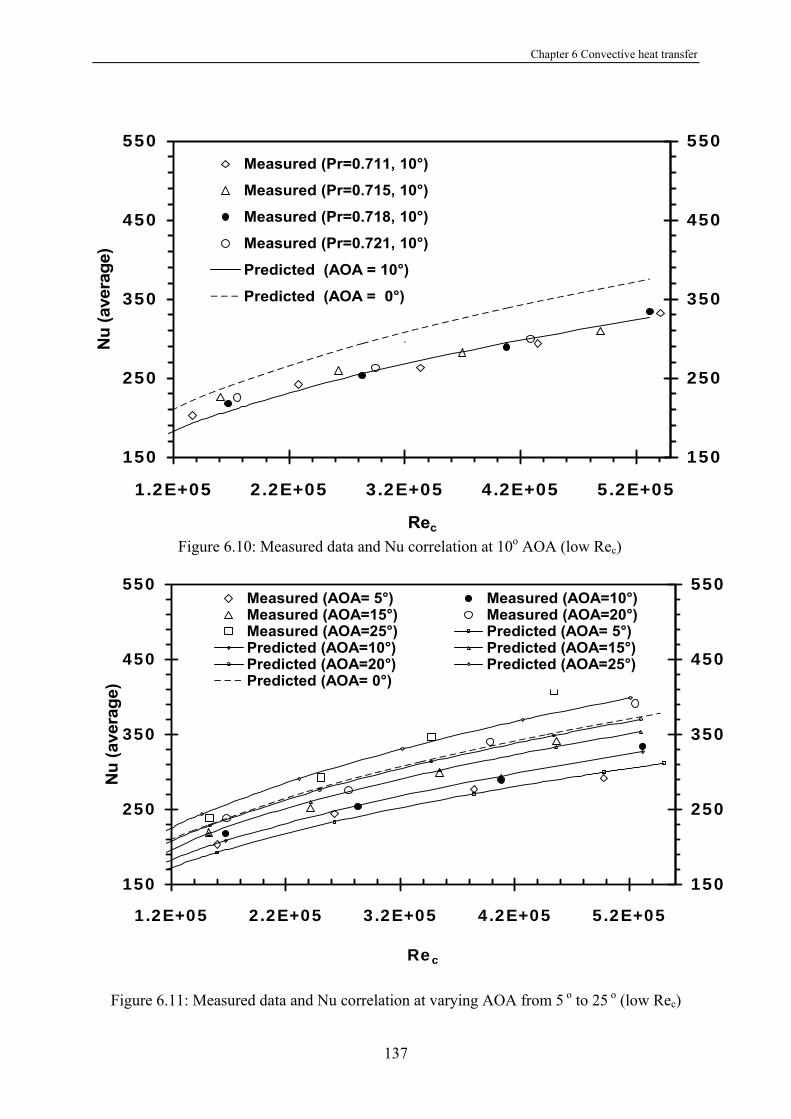
Chapter 6 Convective heat transfer
137
150
250
350
450
550
1.2E+05 2.2E+05 3.2E+05 4.2E+05 5.2E+05
Rec
Nu
(ave
rage
)
150
250
350
450
550Measured (Pr=0.711, 10°)
Measured (Pr=0.715, 10°)
Measured (Pr=0.718, 10°)
Measured (Pr=0.721, 10°)
Predicted (AOA = 10°)
Predicted (AOA = 0°)
`
Figure 6.10: Measured data and Nu correlation at 10o AOA (low Rec)
150
250
350
450
550
1.2E+05 2.2E+05 3.2E+05 4.2E+05 5.2E+05
Rec
Nu
(ave
rage
)
150
250
350
450
550Measured (AOA= 5°) Measured (AOA=10°) Measured (AOA=15°) Measured (AOA=20°)Measured (AOA=25°) Predicted (AOA= 5°)Predicted (AOA=10°) Predicted (AOA=15°)Predicted (AOA=20°) Predicted (AOA=25°) Predicted (AOA= 0°)
Figure 6.11: Measured data and Nu correlation at varying AOA from 5 o to 25 o (low Rec)

Chapter 6 Convective heat transfer
138
The movement of the point of separation depends on the adverse pressure gradient, which
depend on angle of attack and Reynolds number [180]. When the Reynolds number increases,
the separation point moves toward the leading edge. Higher turbulence over the airfoil will
enhance the heat transfer at a higher Reynolds number. Okong'o and Knight [181] predicted
2-D laminar flow over a pitched airfoil, by using a second-order discretization with Roe's
method. The results showed that a larger Reynolds number leads to a primary recirculation
region that forms closer to the leading edge. When the AOA was varied from 14.5° to 22.5°,
the air flow over a NACA 0012 airfoil developed a flow reversal at 14.5°. The primary
recirculation region formed at 16.5°. The primary recirculation region with critical points
formed at 19.5°, while the secondary recirculation region with critical points and primary
recirculation occurred at 21°. A tertiary recirculation region, with secondary recirculation and
critical points, occurred at 22.5°. This implies that a recirculation region developed and
moved towards the leading edge, when the angle of attack increased. The results also showed
that a higher Reynolds number will lead to a circulation region at a smaller angle of attack,
while the centre of recirculation moves forward to the leading edge. The flow and movement
of the point of separation over the NACA 0012 airfoil is different than for the NACA 63421.
These results are helpful to understand the current heat transfer trends along the airfoil at
different AOA and Reynolds numbers.
The following form of correlation has been used for an iced blade by van Foseen [117]:
BcANu Re= (6-8)
where A and B are coefficients that depend on flow conditions. This functional form is similar
to Nu correlations obtained previously by Wang et al. [182] for convective heat transfer from
an airfoil at 0 degrees AOA and associated formula corrections. The relationships between
Reynolds and Nusselt number coefficients (c and m) were determined based on a least squares
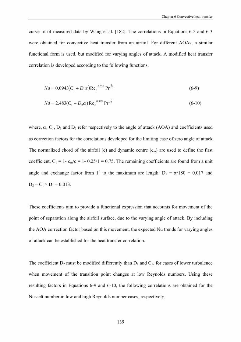
Chapter 6 Convective heat transfer
139
curve fit of measured data by Wang et al. [182]. The correlations in Equations 6-2 and 6-3
were obtained for convective heat transfer from an airfoil. For different AOAs, a similar
functional form is used, but modified for varying angles of attack. A modified heat transfer
correlation is developed according to the following functions,
( ) 31636.0
11 PrRe0943.0 cDCNu α+= (6-9)
31389.0
21 PrRe)(483.2 cDCNu α+= (6-10)
where, α, C1, D1 and D2 refer respectively to the angle of attack (AOA) and coefficients used
as correction factors for the correlations developed for the limiting case of zero angle of attack.
The normalized chord of the airfoil (c) and dynamic centre (cm) are used to define the first
coefficient, C1 = 1- cm/c = 1- 0.25/1 = 0.75. The remaining coefficients are found from a unit
angle and exchange factor from 1o to the maximum arc length: D1 = π/180 = 0.017 and
D2 = C1 × D1 = 0.013.
These coefficients aim to provide a functional expression that accounts for movement of the
point of separation along the airfoil surface, due to the varying angle of attack. By including
the AOA correction factor based on this movement, the expected Nu trends for varying angles
of attack can be established for the heat transfer correlation.
The coefficient D2 must be modified differently than D1 and C1, for cases of lower turbulence
when movement of the transition point changes at low Reynolds numbers. Using these
resulting factors in Equations 6-9 and 6-10, the following correlations are obtained for the
Nusselt number in low and high Reynolds number cases, respectively,
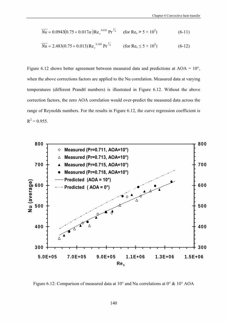
Chapter 6 Convective heat transfer
140
( ) 31636.0 PrRe017.075.00943.0 cNu α+= (for Rec > 5 × 10⁵) (6-11)
31389.0 PrRe)013.075.0(483.2 cNu += (for Rec ≤ 5 × 10⁵) (6-12)
Figure 6.12 shows better agreement between measured data and predictions at AOA = 10°,
when the above corrections factors are applied to the Nu correlation. Measured data at varying
temperatures (different Prandtl numbers) is illustrated in Figure 6.12. Without the above
correction factors, the zero AOA correlation would over-predict the measured data across the
range of Reynolds numbers. For the results in Figure 6.12, the curve regression coefficient is
R2 = 0.955.
300
400
500
600
700
800
5.0E+05 7.0E+05 9.0E+05 1.1E+06 1.3E+06 1.5E+06Rec
Nu
(ave
rage
)
300
400
500
600
700
800Measured (Pr=0.711, AOA=10°)Measured (Pr=0.713, AOA=10°)Measured (Pr=0.715, AOA=10°)Measured (Pr=0.718, AOA=10°)Predicted (AOA = 10°)Predicted ( AOA = 0°)
Figure 6.12: Comparison of measured data at 10° and Nu correlations at 0° & 10° AOA
Chapter 6 Convective heat transfer
141
6.3 Heat transfer characterization with water droplets at 0 AOA
In the previous section, experimental results were presented for convection heat transfer from
a NACA 63421 airfoil at varying Reynolds numbers, by changing the icing tunnel air flow
velocity, air viscosity and thermal diffusivity. In this section, the liquid water content is also
varied. Within the refrigerated wind tunnel in Figure 3.1 and Figure 3.2, air temperatures are
varied between 20oC and -30oC. In addition, liquid droplets are also added to the air. The
quantity of liquid water flow rate varies from 0 to 20 L/h, while the liquid water content
ranges from 0 - 2 g/m3. Data was collected at an air temperature of 10oC with the same
temperature for the air and the water droplets. Data was analyzed over a range of liquid water
contents that yielded uniform normalizations of the Nusselt numbers; this procedure indicated
consistency of the data and provided a useful verification that the experimental data were
collected accurately.
According to the analysis of Section 6.1, experimental data can be correlated by Equations 6.2
and 6.3, in terms of the Nusselt number, which is expressed equivalently to the Hilpert
correlation for an airfoil in cross flow without water droplets, separately for low and high
Reynolds numbers. In this investigation, the liquid water content is expected to substantially
affect the heat transfer coefficient. The average Nusselt number rises by 26.7% and 27.4%,
respectively, for Rec ≤ 5 × 10⁵ and Rec > 5 × 10⁵, relative to the average Nu without water
droplets. In Figure 6.13, it can be noticed that the experimental data has higher values than the
correlation of Nusselt number with Reynolds number, from low to high in Figure 6.13 a) and
b). The correlations of Nu and Re in Figure 6.13 are Eqs. 6-2 and 6-3 for convection heat
transfer from an airfoil. Their modified correlation will be discussed in the following section.
Chapter 6 Convective heat transfer
142
400
450
500
550
600
650
700
750
800
6.0E+05 7.0E+05 8.0E+05 9.0E+05 1.0E+06 1.1E+06Re
Nu
(Ave
rage
)LWC=0.15-0.29
LWC=0.3-0.399
LWC=0.4-0.65
Nu=0.0943Re0.636Pr1/3
a)
200
250
300
350
400
450
500
550
1.0E+05 2.0E+05 3.0E+05 4.0E+05 5.0E+05 6.0E+05Re
Nu
(ave
rage
)
LWC=(0.4-0.49)
LWC=(0.5-0.8)
LWC=(0.9-2)
Nu=2.483
b)
Re0.389Pr1/3
Figure 6.13: Comparison of experimental data with LWC (g/m3) and Nusselt function
correlations without LWC: a) high Re and b) low Re
Rec
Rec

Chapter 6 Convective heat transfer
143
The relationship between Reynolds and Nusselt number coefficients (c and m) are determined
based on a least squares curve fit of measured data. The definition in Equations 6-2 and 6-3
obtained for airfoil heat transfer will be corrected for heat transfer arising from droplet impact
on the airfoil.
Extensions to cases with impinging droplets were made based on correlations in Eqs. 6-2 and
6-3. It was determined that a new multiphase Reynolds parameter, Rem = Rec (1+W), leads to
a promising method of normalizing the experimental data, where W represents a non-
dimensional liquid water content. In other words, the Nusselt number correlation was
established as follows:
31
Pr))1((Rec mc WNu += (6-13)
0
LWCWLWC
= (6-14)
where LWC0 refers to a reference value of the liquid water content. Figure 6.14 shows the local Nusselt numbers, Nux, at different positions and corrected
Reynolds numbers. The stagnation point is x/c = 0. The Nusselt number decreases
significantly after the stagnation point, due to the rapidly thickening boundary layer along the
upper and lower minmium surfaces. It falls to a minmium at a position of 0.2c along the chord
of the airfoil, after which it increases. Although both surfaces of the airfoil have the same
trends near the leading edge of the airfoil, the lowest value of Nux occurs along the lower
surface. It would have the same local Nusselt number, if the airfoil was symmetric in shape
and orientation, with respect to the freestream. The local Nusselt number for the NACA
63421 airfoil has different trends below and above the stagnation point, due to the non-
symmetrical profile of the airfoil. On the airfoil, the thickness of laminar boundary layer
increases as x increases from the leading edge to the trailing edge. Afterwards, boundary layer

Chapter 6 Convective heat transfer
144
transition occurs and the boundary layer becomes turbulent. These trends can be clearly seen
in Figure 6.14.
0
200
400
600
800
1000
1200
1400
-0.6 -0.4 -0.2 0 0.2 0.4 0.6 0.8
Non-dimension position of airfoil based on chord
Nu(
x)
Re(1+W)=235500Re(1+W)=390500Re(1+W)=427300Re(1+W)=516700Re(1+W)=672300Re(1+W)=718900Re(1+W)=819500Re(1+W)=979800
Figure 6.14: Local Nusselt number at varying chord positions (x/c)
By selecting the reference value equal to one-fourth of the maximum water content in air at
the average temperature, it was observed that the same Nusselt number correlation could be
used for both single-phase (without droplets) and two-phase flows (with droplets), provided
the Reynolds number is replaced with the multiphase Reynolds parameter. At the average
temperature of -0.16oC for the low speed set of experiments, the maximum water content in
air is 4.98 g/m3, so the reference water content was taken as 1.25 g/m3. The average
temperature is -4.55oC for the higher speed set of experiments, so the maximum liquid water
content (LWC) at this temperature is 3.69 g/m3 and the reference liquid water content
becomes 0.92 g/m3.
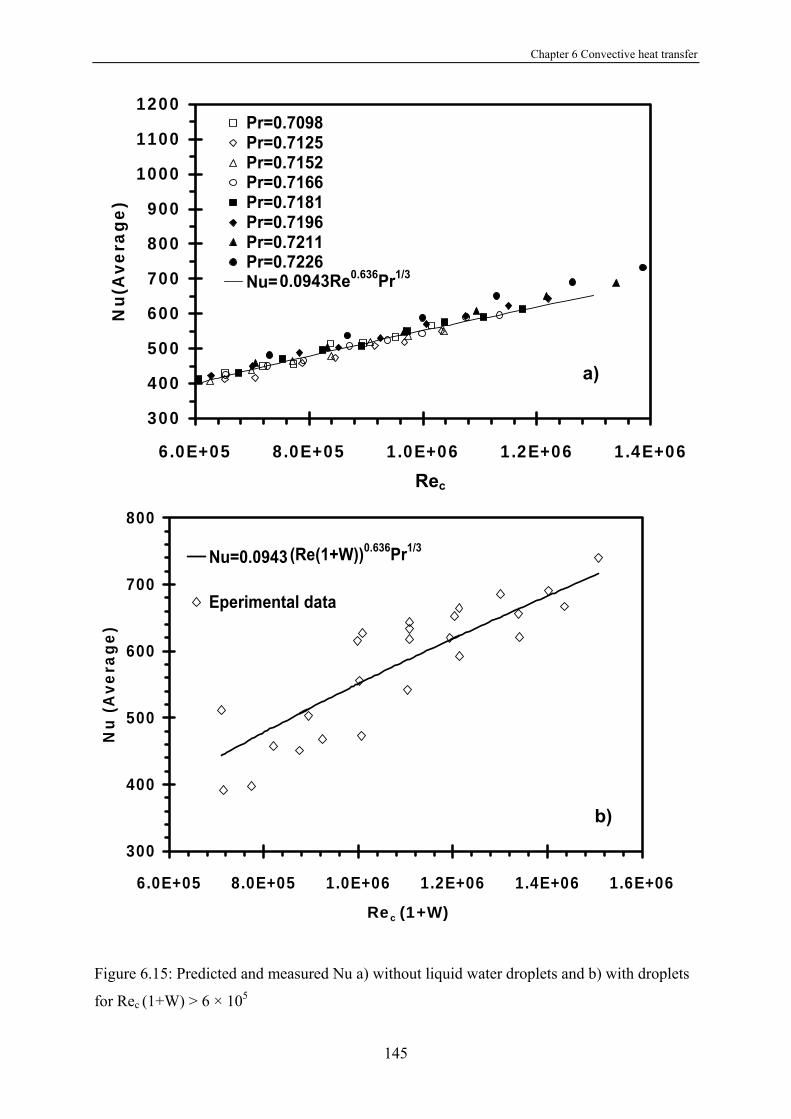
Chapter 6 Convective heat transfer
145
300
400
500
600
700
800
900
1000
1100
1200
6.0E+05 8.0E+05 1.0E+06 1.2E+06 1.4E+06Re
Nu(
Ave
rage
)Pr=0.7098Pr=0.7125Pr=0.7152Pr=0.7166Pr=0.7181Pr=0.7196Pr=0.7211Pr=0.7226Nu=0.0943Re0.636Pr1/3
300
400
500
600
700
800
6.0E+05 8.0E+05 1.0E+06 1.2E+06 1.4E+06 1.6E+06Re(1+W)
Nu
(Ave
rage
)
Nu=0.0943
Eperimental data
(Re(1+W))0.636Pr1/3
Figure 6.15: Predicted and measured Nu a) without liquid water droplets and b) with droplets
for Rec (1+W) > 6 × 10⁵
Rec
a)
b)
Rec (1+W)

Chapter 6 Convective heat transfer
146
200
300
400
500
600
700
800
900
2.0E+05 3.0E+05 4.0E+05 5.0E+05Re
Nu(
Ave
rage
)Pr=0.7098Pr=0.7125Pr=0.7152Pr=0.7166Pr=0.7181Pr=0.7196Pr=0.7211Pr=0.7226Nu=2.483Re0.389Pr1/3
200
300
400
500
2.0E+05 3.0E+05 4.0E+05 5.0E+05Re(1+W)
Nu
(Ave
rage
)
Nu
Expermental data
=2.483(Re(1+W))0.389Pr1/3
Figure 6.16: Predicted and measured Nu a) without liquid water droplets and b) with droplets
for Rec (1+W) ≤ 6 × 10⁵
Rec
Rec (1+W)
b)
a)
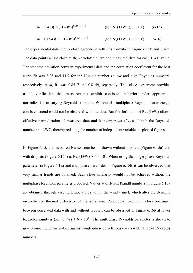
Chapter 6 Convective heat transfer
147
31389.0 Pr))1((Re483.2 WNu c += (for Rec(1+W) ≤ 6 × 10⁵) (6-15)
31636.0 Pr))1((Re0943.0 WNu c += (for Rec(1+W) > 6 × 10⁵) (6-16)
The experimental data shows close agreement with this formula in Figure 6.15b and 6.16b.
The data points all lie close to the correlated curve and measured data for each LWC value.
The standard deviation between experimental data and the correlation coefficient for the best
curve fit was 8.25 and 11.9 for the Nusselt number at low and high Reynolds numbers,
respectively. Also, R2 was 0.8517 and 0.8149, separately. This close agreement provides
useful verification that measurements exhibit consistent behavior under appropriate
normalization at varying Reynolds numbers. Without the multiphase Reynolds parameter, a
consistent trend could not be observed with the data. But the definition of Rec (1+W) allows
effective normalization of measured data and it incorporates effects of both the Reynolds
number and LWC, thereby reducing the number of independent variables in plotted figures.
In Figure 6.15, the measured Nusselt number is shown without droplets (Figure 6.15a) and
with droplets (Figure 6.15b) at Rec (1+W) > 6 × 10⁵. When using the single-phase Reynolds
parameter in Figure 6.15a and multiphase parameter in Figure 6.15b, it can be observed that
very similar trends are obtained. Such close similarity would not be achieved without the
multiphase Reynolds parameter proposed. Values at different Prandtl numbers in Figure 6.15a
are obtained through varying temperatures within the wind tunnel, which alter the dynamic
viscosity and thermal diffusivity of the air stream. Analogous trends and close proximity
between correlated data with and without droplets can be observed in Figure 6.16b at lower
Reynolds numbers (Rec (1+W) ≤ 6 × 10⁵). The multiphase Reynolds parameter is shown to
give promising normalization against single-phase correlations over a wide range of Reynolds
numbers.

Chapter 6 Convective heat transfer
148
Several key differences should be noted between Figure 6.13, Figure 6.15 and Figure 6.16. In
Figure 6.13, measured data is shown at different values of the liquid water content (two-phase
flow with droplets), while Figure 6.15a and Figure 6.16a show Nusselt numbers at varying
temperatures and Prandlt numbers (without droplets). The measured data in Figure 6.15a and
Figure 6.16a was used to develop the empirical correlations Eqs. 6-2 and 6-3 in Figure 6.13.
Also, Figure 6.15b and Figure 6.16b plot the Nusselt numbers against the multiphase
Reynolds parameter, while Figure 6.13 plots the Nusselt number against the conventional,
single-phase Reynolds number (without droplets) obtained in Section 6.1. The results in
Figure 6.15b and Figure 6.16b are nearly independent of the Prandtl number, since the
temperature range and variations of the Prandtl number are small. The data is the same as
results in Figure 6.13a and b, except that it is normalized by LWC0 and plotted against the
multiphase Reynolds parameter, rather than the conventional single-phase Reynolds number.
The number of measured data points in Figure 6.13, Figure 6.15 and Figure 6.16 is different
since the Reynolds number on the horizontal axis is different, thereby affecting the number of
data points within a given range.
6.4 Modified hilpert correlation with LWC at varying AOA
In this section, experimental results will be presented for convective heat transfer from a
NACA 63421 airfoil at varying AOA between 0° and 25°. The Reynolds number is varied by
changing the air velocity in the icing tunnel and air viscosity (by changing the air
temperature). The liquid water content is also varied through different spray flow conditions.
Within the refrigerated wind tunnel, air temperatures are varied between -30oC and 20oC. The
liquid water content varies from 0 to 45 liters per hour. Data is collected over a range of
temperatures and liquid water contents that yielded uniform normalization of the Nusselt

Chapter 6 Convective heat transfer
149
numbers. For example, normalized data collapsed onto a single curve fit at different
temperatures which indicated consistency and provided useful verification that experimental
data was collected accurately.
Particular effort was taken to ensure uniformity of the droplet distribution. Atomizing nozzles
were adjusted iteratively with the air and water streams to improve the uniformity. This was a
time-consuming process, since they affect each other. Also, Particle Image Velocimetry (PIV)
was used to analyze the uniformity of the droplet distribution at each step. Furthermore, icing
patterns were observed on the airfoil and the uniformity of ice buildup provided another way
to improve uniformity of the droplet distribution. These efforts and others were taken to
provide as uniform a droplet distribution as possible.
From the manufacturer’s specifications of the spray nozzles, the average droplet size is 100
microns. The air atomizing nozzles can produce a reliable spray pattern with water mean
droplet diameters ranging between 10 and 1,000 microns. At the nozzle exit, droplet ejection
is air-assisted since the air stream drives the emission from the nozzle, rather than ejection at a
particular velocity, so the droplet velocity is close to the air stream velocity. Droplet sizes are
controlled by variation of the air pressure. Figure 6.17 compares the measured data and
correlations for both high and low Reynolds numbers at a 15o angle of attack. The results
illustrate that the average Nusselt number increases at a higher Reynolds number. Measured
data at varying temperatures (different Prandtl numbers) is illustrated in the figure. For the
low Reynolds number, without the AOA correction factors developed in the previous section,
the zero AOA correlation would over-predict the measured data across the range of Reynolds
numbers. The AOA correction to the Hilpert correlation was determined empirically from the
curve fit of measured data.
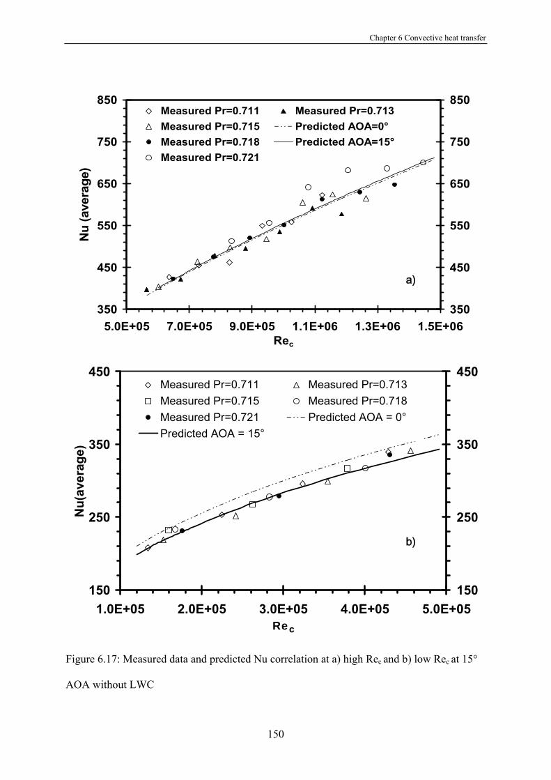
Chapter 6 Convective heat transfer
150
350
450
550
650
750
850
5.0E+05 7.0E+05 9.0E+05 1.1E+06 1.3E+06 1.5E+06Rec
Nu
(ave
rage
)
350
450
550
650
750
850Measured Pr=0.711 Measured Pr=0.713Measured Pr=0.715 Predicted AOA=0°Measured Pr=0.718 Predicted AOA=15°Measured Pr=0.721
150
250
350
450
1.0E+05 2.0E+05 3.0E+05 4.0E+05 5.0E+05Rec
Nu(
aver
age)
150
250
350
450Measured Pr=0.711 Measured Pr=0.713Measured Pr=0.715 Measured Pr=0.718Measured Pr=0.721 Predicted AOA = 0°Predicted AOA = 15°
Figure 6.17: Measured data and predicted Nu correlation at a) high Rec and b) low Rec at 15°
AOA without LWC
a)
b)

Chapter 6 Convective heat transfer
151
Results of measured data at various values of the LWC are plotted in Figure 6.18, together
with a correlated curve fit of experimental data without water droplets, which was derived by
conducting the experiments at the same operating AOA, but with the spray nozzles closed. In
Figure 6.18, the solid curves represent empirical correlations without droplets when angle of
attack α = 15°. The markers correspond to measured data with droplets at 15° AOA and the
dotted line illustrates predictions of the Nusselt number with the multiphase Reynolds
parameter, Rec(1+W). The curve of Eq. 6-12 in Figure 6.18 has a higher Reynolds number
due to the data modification by (1+W). Neither the correlation of Nusselt number and
Reynolds number in Eq. 6-11, nor Eq. 6-16, can be used to predict the heat transfer
correlation with liquid water droplets at varying AOA, although the multiphase Reynolds
number can be used to include effects on the heat transfer coefficient. A new heat transfer
coefficient is needed in this situation. The experimental data indicates that the average Nusselt
number at a fixed AOA rises about 26.4% for Rec > 6 × 10⁵, when water droplets are
introduced into the air stream. Impinging droplets enhance the rate of heat exchange between
the surface and air stream, as they enhance fluid mixing along the wall, thereby increasing the
convective heat exchange and Nusselt number.
Experimental results show that the angle of attack substantially affects the heat transfer
coefficient, both with and without water droplets. Figure 6.19 shows the measured local
Nusselt numbers, Nux, at different positions with a LWC of 0.58 g/m3 and 0.75 g/m3 at high
and low Re. The stagnation point is located at x/c = 0. The curve with AOA = 0 shows that
the Nusselt number decreases after the stagnation point, due to the thickening boundary layer
along the top and bottom surfaces. It falls to a minimum point at a position of 0.2c along the
chord of the airfoil, and then increases thereafter. Although both surfaces of the airfoil have
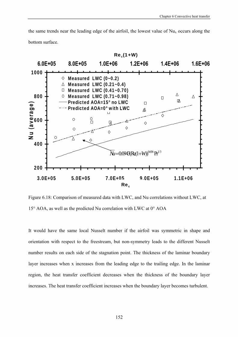
Chapter 6 Convective heat transfer
152
the same trends near the leading edge of the airfoil, the lowest value of Nux occurs along the
bottom surface.
200
400
600
800
1000
3.0E+05 5.0E+05 7.0E+05 9.0E+05 1.1E+06Re
Nu
(ave
rage
)
6.0E+05 8.0E+05 1.0E+06 1.2E+06 1.4E+06 1.6E+06Re(1+W)
Measured LWC (0~0.2)Measured LWC (0.21~0.4)Measured LWC (0.41~0.70)Measured LWC (0.71~0.98)Predicted AOA=15° no LWCPredicted AOA=0° with LWC
0.636 1/30.0943(Re(1 )) PrNu W= +
Figure 6.18: Comparison of measured data with LWC, and Nu correlations without LWC, at
15° AOA, as well as the predicted Nu correlation with LWC at 0° AOA
It would have the same local Nusselt number if the airfoil was symmetric in shape and
orientation with respect to the freestream, but non-symmetry leads to the different Nusselt
number results on each side of the stagnation point. The thickness of the laminar boundary
layer increases when x increases from the leading edge to the trailing edge. In the laminar
region, the heat transfer coefficient decreases when the thickness of the boundary layer
increases. The heat transfer coefficient increases when the boundary layer becomes turbulent.
Rec
Rec(1+W)

Chapter 6 Convective heat transfer
153
In Figure 6.19a, it can be observed how the local Nu changes with AOA at LWC = 0.75 g/m3,
for cases of low Reynolds numbers. At the stagnation point, the Nusselt number changes with
LWC. Without droplets in the air stream, it remains nearly uniform at different values of
AOA, whereas the Nusselt number increases higher than AOA = 0 with a non-zero LWC,
although it doesn’t depend on the angle of attack. It also changes significantly with AOA
along the chord of the airfoil. The Nusselt number decreases at ± 0.1c, -0.4c, 0.6c and it
significantly increases at -0.2c, -0.6c and +0.4c and +0.8c. Figure 6.19b shows the Nusselt
number results for cases of high Reynolds numbers at various AOA and LWC = 0.51 g/m3. At
angles of attack of 5°, the local Nusselt number at the stagnation point is lower than the case
for 20° and 25°, but higher than the case for 10° and 15°.
All values of the Nusselt number at the stagnation point are higher than the case for 0° AOA.
Values of the Nusselt number at -0.1c, +0.1c and +0.6c change depending on the AOA at
those points. The values at -0.2c, -0.6c, +0.2c and +0.4c are higher than a zero AOA at the
same points. As AOA increases, the changes of local Nu with AOA become more pronounced
at higher Reynolds numbers. Also, no points of the local Nusselt number along the chord of
the airfoil have lower values than the Nusselt number at 0° for the same points. Furthermore,
Nux for the other points along the chord of the airfoil are larger than the values at the same
points for 0°. The average Nusselt number is expected to have similar trends at high
multiphase Reynolds numbers.

Chapter 6 Convective heat transfer
154
0
400
800
1200
1600
2000
-1 -0.8 -0.6 -0.4 -0.2 0 0.2 0.4 0.6 0.8 1Dimensionless Chord (C)
Nux
AOA=0° Re=320000 AOA=5° Re=350000AOA=10° Re=360000 AOA=15° Re=350000AOA=20° Re=350000 AOA=25° Re=340000
a)
Bottom surface Top surface
100
500
900
1300
1700
2100
2500
2900
-1 -0.8 -0.6 -0.4 -0.2 0 0.2 0.4 0.6 0.8 1Dimensionless Chord (C)
Nux
AOA=0° Re=850000 AOA=5° Re=870000AOA=10° Re=870000 AOA=15° Re=870000AOA=20° Re=860000 AOA=25° Re=860000
b)
Bottom surface Top surface
Figure 6.19: Nusselt number at a) low Reynolds numbers with LWC = 0.75 g/m3 and b) high
Reynolds numbers with LWC = 0.51 g/m3 at varying AOA

Chapter 6 Convective heat transfer
155
The results also showed that a higher Reynolds number will lead to a circulation region at the
smaller angle of attack, while the centre of recirculation moves forward to the leading edge.
These mechanisms of the recirculation zone affect the convective heat exchange, so the
Nusselt correlation requires a suitable dependence on AOA, which reflects the physical
processes in the boundary layer. A modified Hilpert correlation is used to fit measured data
obtained from the experiments according to Eqs. 6-11 and 6-12 to 6-15 and 6-16 as follows:
31389.0
c31 Pr))1()(Re(483.2 WDCNu ++= α , and (6-17)
31636.0
42 Pr))1()(Re(0943.0 WDCNu c ++= α , (6-18)
Where, α, C1, C2, D3 and D4 refer to the angle of attack (AOA) and coefficients used as
correction factors for the correlations developed in the limiting case of zero angle of attack.
The normalized chord of the airfoil, c, and dynamic centre, cm, are used to define the first
coefficient, C1= 1 - cm/c = 1 - 0.25/1 = 0.75. The remaining coefficients are found from a unit
angle and exchange factor from 1o to the maximum arc length: π/180 = 0.017 and D3 = C12 ×
0.017 = 0.01. These coefficients provide a functional expression that accounts for movement
of the point of separation along the airfoil surface, due to the varying angle of attack.
The coefficient D4 must be modified differently by D3 and C1, for cases of higher turbulence
to decrease the effect of the angle of attack under conditions of impinging droplets.
Movement of the transition point changes at high Reynolds numbers, so D4 = C1 × D3 = 0.007.
The other chord coefficient is: C2 = c/c = 1. Higher turbulence increases the heat transfer
coefficient in droplet flow conditions, regardless of the angle of attack. Using the resulting
factors in Eqs. 6-17 and 6-18, the following correlations are obtained for the Nusselt number
in low and high Reynolds number cases, respectively,
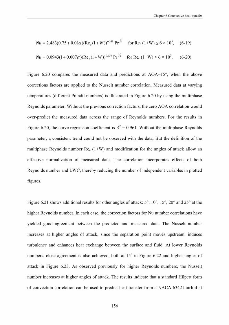
Chapter 6 Convective heat transfer
156
31389.0 Pr))1()(Re01.075.0(483.2 WNu c ++= α for Rec (1+W) ≤ 6 × 10⁵, (6-19)
31636.0 Pr))1()(Re007.01(0943.0 WNu c ++= α for Rec (1+W) > 6 × 10⁵. (6-20)
Figure 6.20 compares the measured data and predictions at AOA=15°, when the above
corrections factors are applied to the Nusselt number correlation. Measured data at varying
temperatures (different Prandtl numbers) is illustrated in Figure 6.20 by using the multiphase
Reynolds parameter. Without the previous correction factors, the zero AOA correlation would
over-predict the measured data across the range of Reynolds numbers. For the results in
Figure 6.20, the curve regression coefficient is R2 = 0.961. Without the multiphase Reynolds
parameter, a consistent trend could not be observed with the data. But the definition of the
multiphase Reynolds number Rec (1+W) and modification for the angles of attack allow an
effective normalization of measured data. The correlation incorporates effects of both
Reynolds number and LWC, thereby reducing the number of independent variables in plotted
figures.
Figure 6.21 shows additional results for other angles of attack: 5°, 10°, 15°, 20° and 25° at the
higher Reynolds number. In each case, the correction factors for Nu number correlations have
yielded good agreement between the predicted and measured data. The Nusselt number
increases at higher angles of attack, since the separation point moves upstream, induces
turbulence and enhances heat exchange between the surface and fluid. At lower Reynolds
numbers, close agreement is also achieved, both at 15o in Figure 6.22 and higher angles of
attack in Figure 6.23. As observed previously for higher Reynolds numbers, the Nusselt
number increases at higher angles of attack. The results indicate that a standard Hilpert form
of convection correlation can be used to predict heat transfer from a NACA 63421 airfoil at
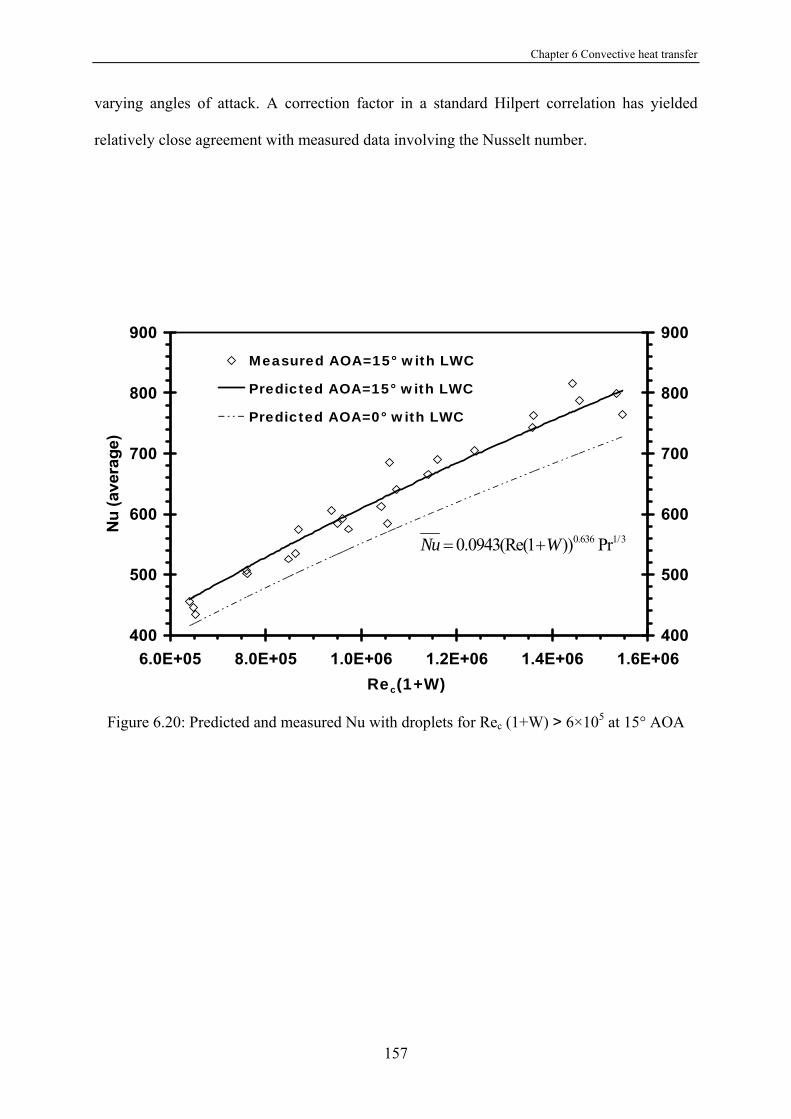
Chapter 6 Convective heat transfer
157
varying angles of attack. A correction factor in a standard Hilpert correlation has yielded
relatively close agreement with measured data involving the Nusselt number.
400
500
600
700
800
900
6.0E+05 8.0E+05 1.0E+06 1.2E+06 1.4E+06 1.6E+06Re(1+W)
Nu
(ave
rage
)
400
500
600
700
800
900Measured AOA=15° with LWC
Predicted AOA=15° with LWC
Predicted AOA=0° with LWC
0.636 1/30.0943(Re(1 )) PrNu W= +
Figure 6.20: Predicted and measured Nu with droplets for Rec (1+W) > 6×10⁵ at 15° AOA
Rec(1+W)
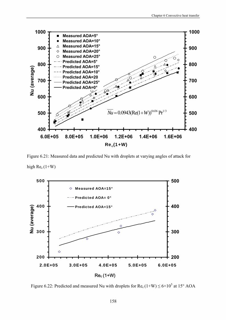
Chapter 6 Convective heat transfer
158
400
500
600
700
800
900
1000
6.0E+05 8.0E+05 1.0E+06 1.2E+06 1.4E+06 1.6E+06Re(1+W)
Nu
(ave
rage
)
400
500
600
700
800
900
1000Measured AOA=5°Measured AOA=10°Measured AOA=15° Measured AOA=20°Measured AOA=25°Predicted AOA=5°Predicted AOA=15°Predicted AOA=10°Predicted AOA=20Predicted AOA=25°Predicted AOA=0°
0.636 1/30.0943(Re(1 )) PrNu W= +
Figure 6.21: Measured data and predicted Nu with droplets at varying angles of attack for
high Rec (1+W)
200
300
400
500
2.0E+05 3.0E+05 4.0E+05 5.0E+05 6.0E+05
Re(1+W)
Nu
(ave
rage
)
200
300
400
500Measured AOA=15°
Predicted AOA= 0°
Predicted AOA=15°
Figure 6.22: Predicted and measured Nu with droplets for Rec (1+W) ≤ 6×10⁵ at 15° AOA
Rec(1+W)
Rec (1+W)
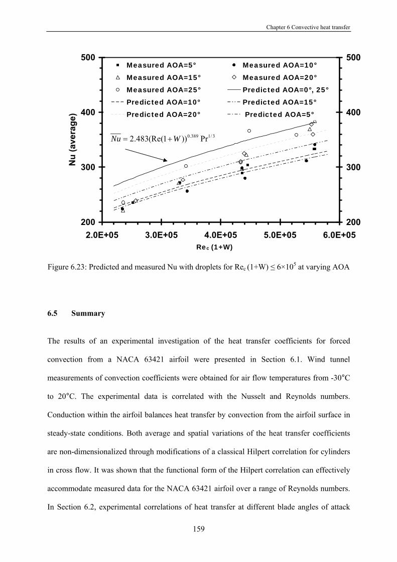
Chapter 6 Convective heat transfer
159
200
300
400
500
2.0E+05 3.0E+05 4.0E+05 5.0E+05 6.0E+05Re(1+W)
Nu
(ave
rage
)
200
300
400
500Measured AOA=5° Measured AOA=10°
Measured AOA=15° Measured AOA=20°Measured AOA=25° Predicted AOA=0°, 25°
Predicted AOA=10° Predicted AOA=15°Predicted AOA=20° Predicted AOA=5°
0.389 1/ 32.483(Re(1 )) PrNu W= +
Figure 6.23: Predicted and measured Nu with droplets for Rec (1+W) ≤ 6×10⁵ at varying AOA
6.5 Summary
The results of an experimental investigation of the heat transfer coefficients for forced
convection from a NACA 63421 airfoil were presented in Section 6.1. Wind tunnel
measurements of convection coefficients were obtained for air flow temperatures from -30°C
to 20°C. The experimental data is correlated with the Nusselt and Reynolds numbers.
Conduction within the airfoil balances heat transfer by convection from the airfoil surface in
steady-state conditions. Both average and spatial variations of the heat transfer coefficients
are non-dimensionalized through modifications of a classical Hilpert correlation for cylinders
in cross flow. It was shown that the functional form of the Hilpert correlation can effectively
accommodate measured data for the NACA 63421 airfoil over a range of Reynolds numbers.
In Section 6.2, experimental correlations of heat transfer at different blade angles of attack
Rec (1+W)
Chapter 6 Convective heat transfer
160
(NACA 63421 airfoil) were developed. Various angels of attack (AOA) between 0 to 25
degrees were investigated at different Reynolds numbers. The correlations provide important
characterization of convective heat transfer from the airfoil surface to the cold surrounding air.
Experimental studies of heat transfer with water droplets impinging on a NACA 63421 airfoil
were studied to simulate anti-icing conditions in Section 6.3. Various liquid water contents
(LWC) were investigated. The measurements can provide important characterization of heat
convection between the airfoil surface and cold surrounding air, just before ice accumulation.
These experimental measurements can be used to develop better methods to reduce the impact
of icing of wind turbines in cold weather climates.
A new non-dimensional correlation of convective heat transfer with impinging droplets on a
NACA airfoil at varying angles of attack was presented in Section 6.4. The experimental
study was performed to develop correlations of heat transfer from a NACA 63421 airfoil at
different angles of attack (AOA) between 0 to 25 degrees and different Reynolds numbers
with impinging droplets. A modified Hilpert correlation of convective droplet heat transfer
from the NACA airfoil at varying AOA was determined with respect to the Reynolds number,
Prandtl number, liquid water content and AOA. The modified Hilpert correlation includes the
effects of droplet-air interactions on the effective heat transfer coefficient at varying AOA.
Increasing the AOA leads to flow separation and reattachment on the airfoil surface, which
affect the structure of the thermal boundary layer and energy exchange through kinetic energy
of impinging droplets and the thin flowing film along the surface of the airfoil. The results
show that both average and local Nusselt numbers vary with AOA. The results indicates that
variation of air velocity, liquid water content and AOA can be normalized into a modified
Hilpert correlation, by using empirical coefficients that involve the chord dimensions, AOA
and non-dimensional liquid water content.

161
Chapter 7
Conclusions and recommendations for future research
7.1 Conclusions
Iced wind turbine blades and convective heat transfer from a NACA airfoil were investigated
in this thesis. In this chapter, conclusions will be presented for the following aspects of wind
energy: wind power losses under icing conditions, aerodynamic losses under icing conditions
and convective heat transfer at varying AOA, with or without LWC.
The experimental results presented in Chapter 4 show that icing of a wind turbine blade will
significantly affect power output. Normally, glaze ice will reduce power output progressively
as the ice thickness increases. Extreme cold temperatures will form a larger thickness of rime
ice on the blades, for the same icing duration, compared to glaze ice conditions. Rime ice that
forms on the wind turbine blades will change the profile of the wind turbine blades and these
iced blades may increase their rotation rate under extreme ice conditions. For experimental
icing conditions, the power output increased to 214% with 8.5 mm of rime ice thickness and
the rotation rate of the wind turbine increased to 125% at -30°C. This is dangerous for the
wind turbine because the high rotation speed and increased power output may cause the
mechanical and electrical parts to overheat and fail. Power losses and high rotation are two
consequences of iced wind turbine blades in extreme climates.
Chapter 7 Conclusions and recommendations
162
The iced airfoil aerodynamics affects the power output, due to the changing blade profile.
From the ice shapes on an airfoil, glaze ice conditions will form smoother ice over the airfoil
than rime ice conditions. Also, the ice thickness for the same spraying duration is different,
due to the difference of air temperatures. When the temperature is lower, the ice thickness will
be large. The lift coefficient and drag coefficient are also changing, as glaze ice conditions
and rime ice conditions change. The aerodynamics of an iced airfoil was slightly affected by
the higher Reynolds number. When the Reynolds number is lower, the lift coefficient of an
iced airfoil will decrease, more than the higher Reynolds number, at the same ice thickness.
Also, the rime ice and glaze ice have different effects on drag and lift coefficients, when
varying the Reynolds number, spraying time and AOA.
Heat transfer results were presented in Chapter 6, including modified Hilpert correlations to
predict heat transfer by forced convection from a NACA airfoil, with and without LWC, at 0
and varying AOA. Initially, a modified Hilpert correlation was used for heat transfer by
forced convection from a NACA airfoil at zero AOA, without liquid water content. Under
steady-state conditions, heat conduction through the airfoil was balanced against heat transfer
by convection to the air stream. Experimental data was shown to collapse consistently onto a
single normalized correlation of Nu/Pr1/3 at varying Prandtl numbers. Representative
coefficients of the modified Hilpert correlation were obtained. It was observed that the
average Nusselt number for an airfoil is smaller than a flat plate and cylinder at the same
Reynolds number, as a result of the differences between turbulent boundary layer behaviors
after the transition point.
A modified Hilpert correlation of forced convection heat transfer from the NACA airfoil was
presented for different angles of attack. An experimental method was developed with
Chapter 7 Conclusions and recommendations
163
thermocouples embedded at different locations along the surface of the airfoil. Representative
coefficients of the modified Hilpert correlation were reported. The modifications of AOA are
(0.75 + 0.013α) and (0.75 + 0.0017α), separately for low and high Reynolds numbers,
respectively. It was observed that the average Nusselt number varied with angles of attack,
due to movement of the transition point and turbulence. The correction factors and modified
correlations have provided useful new predictive tools for convective heat transfer from
airfoils at varying angles of attack.
Results were presented on the investigation of heat transfer coefficients for forced convection
from the NACA airfoil with effects of impinging liquid water droplets. Wind tunnel
measurements of the convection coefficients were obtained for air flows with LWC ranging
from 0 - 2 g/m3 at AOA = 0. The experimental data were correlated with the Nusselt and
Reynolds numbers. Both average and spatial variations of the heat transfer coefficients were
non-dimensionalized through modifications of the Hilpert correlation for cylinders in cross
flow, while the Reynolds number was corrected by the LWC. The corrected W = LWC/LWC0
uses LWC0 = 0.92 for LWC less than 1 g/m3 and LWC0 = 1.25 when LWC ranges from 1 to
2 g/m3.
Another experimental study of heat transfer was conducted for forced convection with droplet
impact on the NACA 63421 airfoil at varying angles of attack from 5o to 25o. Wind tunnel
studies were conducted at varying wind speeds and LWC values ranging between 0 - 2 g/m3.
The experimental data were correlated with the Nusselt number, angle of attack and a newly
defined multiphase Reynolds number. Both average and local Nusselt numbers were obtained
and non-dimensionalized in a modified Hilpert correlation. An uncertainty analysis was
performed to give a measurement uncertainty of 7.34% for the measured Nusselt numbers,

Chapter 7 Conclusions and recommendations
164
(Appendix B – Measurement uncertainties). The new correlations have provided useful new
predictive tools for convective heat transfer from airfoils, with and without LWC, at varying
AOA.
7.2 Recommendations for future research
The following suggestions are recommended for further study of aerodynamics and heat
transfer related to wind turbine icing.
1. The LWC and MVD in the wind tunnel should be tested further with
experimental facilities. They affect the results significantly. Uniform droplet sizes
are important for the aerodynamic investigation.
2. The aerodynamics experiment of the iced airfoil should be investigated further
with two end plates within the tunnel. A 2-D or 3-D investigation for the airfoil is
different. The 3-D experiments have different values, due to the side effects, than
2-D airfoil investigations.
3. Flow visualization of the airfoil at various AOA in a water tunnel would be
helpful for the flow field over the airfoil. This would provide deeper insight for
more understanding of the convective heat transfer coefficient, when air flow
passes over the blade.
4. An infrared Temperature Measurement System is a possible method to measure
surface temperatures of an iced airfoil. A combined temperature measurement
system, with thermocouples inside the airfoil, can be used to obtain the heat
transfer coefficient of the iced airfoil.
5. An iced airfoil will be tested over a very short time to compare an un-iced airfoil
and iced airfoil. Results obtained from an iced airfoil indicate that the spraying

Chapter 7 Conclusions and recommendations
165
time affects the aerodynamics. A minute or a shorter time test would disclose ice
accretion information with a high speed camera.
6. Computer simulation studies with CFD for the iced airfoil would be helpful to
simulate various ice conditions.

166
References
[1] EWEA (the European Wind Energy Association), “Green Peace International, Wind
Force 12 A blueprint to achieve 12% of the world‘s electricity from wind power by
2020,” June 2005. http://www.greenpeace.org/international/press/reports/windforce-
12-2005. Accessed on Feb. 06, 2006.
[2] GWEC (Global Wind Energy Council), Global wind 2007 report.
http://www.gwec.net/uploads/media/Global_Wind_2007_Report_final.pdf. Accessed
on May 17, 2008.
[3] GWEC (Global Wind Energy Council),
http://www.gwec.net/index.php?id=30&no_cache=1&tx_ttnews[pointer]=1&tx_ttnew
s[tt_news]=24&tx_ttnews[backPid]=4&cHash=26e173f378. Accessed on June 06,
2006.
[4] Canadian Wind Energy Association
http://www.canwea.ca/images/uploads/File/WindSight/windsight_jul07.pdf. Accessed
on Sep. 07, 2007.
[5] T. Laakso, E. Peltola, “A statistical evaluation of icing and low temperature failures in
Finland 1996 – 2002,” BOREAS VI Proceedings, April 2003.
[6] G. Ronsten, “Svenska erfarenheter av vindkraft i kallt klimat—nedisning, iskast och
avisning,” Elforsk rapport 04:13, May, 2004.
[7] J. Druez, D.D. Nguyen, Y. Lavoie, “Mechanical properties of atmospheric ice,” Cold
Region Science and technology, vol. 13, pp. 67 - 74, 1986.

References
167
[8] EWEA, “Prioritizing wind energy research strategic research agenda of the wind
energy sector. July 2005.” http://www.ewea.org/index.php?id=15. Accessed on 06.02,
2006.
[9] IEA, “2005 IEA Wind Energy Annual Report”. http://ieawind.org/ar_two_o_five.html.
Accessed on July 16, 2006.
[10] Wind energy in the NWT and Nunavut, “Arctic experience”,
http://www.yec.yk.ca/wind/presentations/May%2027/Project%20Development%20&
%20Success%20Stories%20II/SteveKerr%20LeeDouglas%20Wind%20Energy%20-
%20NWT%20and%20Nunavut.pdf, Accessed on July 28, 2006.
[11] J. Woods, “Ice & wind factors in wind turbine output in Southern Manitoba,” report to
Manitoba Hydro, 2007.
[12] T. Laakso, “Wind energy projects in cold climates,” report to the Executive
Committee of the International Energy Agency Programme, edition 2005.
[13] http://virtual.vtt.fi/virtual/arcticwind/. Accessed on September 12, 2007.
[14] http://www.lmglasfiber.com/News/Archive/View%20News.aspx?id=0DEFA898-
82D4-4662-9BAF-B3E66570D2A6&y=2007. Accessed on Sep.11, 2007.
[15] EWEA, “Execute summary, wind energy the facts, An analysis of wind energy in the
EU-25,” http://www.ewea.org/index.php?id=91&no_cache=1&sword_list[]=facts.
Accessed on Sep. 12, 2007.
[16] F. N. Coton, T. Wang, R. A. McD. Galbraith, “An examination of key aerodynamic
modelling issues raised by the NREL blind comparison,” Wind Energy, vol. 5, pp. 199
- 212, 2002.
[17] Y. U. Sohn, Ch. H. Chun, Y. C. Kim, C. W. Chung, Y. H. Kim, K. S. Han, J. Y. Ryu,
D. H. Kim, R. Schmidt, M. Rees, “Blade design of a 750 kW direct-drive wind
turbine generator system,”
References
168
http://scholar.google.com/scholar?hl=en&lr=&q=related:FJBZ26E8mZsJ:scholar.goo
gle.com/. Accessed on Aug 21, 2007.
[18] C. Kong, J. Bang, Y. Sugiyama, “Structural investigation of composite wind turbine
blade considering various load cases and fatigue life,” Energy, vol. 30, pp. 2101 -
2114, 2005.
[19] K. J. Jackson, M. D. Zuteck, C. P. van Dam, K. J. Standish, D. Berry, “Innovative
design approaches for large wind turbine blades,” Wind Energy, vol. 8. pp. 141 - 171,
2005.
[20] P. Fuglsang, C. Bak, “Development of the Risø wind turbine airfoils,” Wind Energy.
vol. 7, pp. 145 - 162, 2004.
[21] C. Bak, P. Fuglsang, “Modification of the NACA 622-415 leading edge for better
aerodynamic performance,” Journal of Solar Energy Engineering, vol. 124, pp. 327 -
334, 2002.
[22] I. Grant, M. Mo, X. Pan, P. Parkin, J. Powell, H. Reinecke, K. Shuang, F. Coton, D.
Lee, “An experimental and numerical study of the vortex filaments in the wake of an
operational, horizontal-axis, wind turbine,” Journal of Wind Engineering and
Industrial Aerodynamics, vol. 85, no. 2, pp. 177 - 189, 2000.
[23] S. Schreck and M. Robinson, “Rotational augmentation of horizontal axis wind
turbine blade aerodynamic response,” Wind Energy, vol. 5, pp. 133 - 150, 2002.
[24] W. A. Timmer, A. P. Schaffarczyk, “The effect of roughness at high Reynolds
Numbers on the performance of aerofoil DU 97-W-300Mod,” Wind Energy, vol. 7, pp.
295 - 307, 2004.
[25] K. Y. Maalawi, H. M. Negm, “Optimal frequency design of wind turbine blades,”
Journal of Wind Engineering and Industrial Aerodynamics, vol. 90, pp. 961 - 986,
2002.
References
169
[26] J. M. Mejía, F. Chejne, R. Smith, L. F. Rodríguez, O. Fernández, I. Dyner, “Technical
note simulation of wind energy output at Guajira, Colombia,” Renewable Energy, vol.
31, pp. 383 - 399, 2006.
[27] M. Jureczko, M. Pawlak, A. Mężyk, “Optimization of wind turbine blades,” Journal
of Materials Processing Technology, vol. 167, pp. 463 - 471, 2005.
[28] Norwin 46/47-ASR-600/750KW Main feature of design,
http://www.norwinna.com/turbine_750.htm. Accessed on Oct 12, 2007.
[29] J. S. R. Anttonen, P. I. King, P. S. Beran, “Applications of multi-POD to a pitching
and plunging airfoil,” Mathematical and Computer Modeling, vol. 42, pp. 245 - 259,
2005.
[30] R. Giering, T. Kaminski, T. Slawig, “Generating efficient derivative code with TAF
adjoint and tangent linear Euler flow around an airfoil,” Future Generation Computer
Systems, vol. 21, pp. 1345 - 1355, 2005.
[31] S. Mittal, P. Saxena, “Hysteresis in flow past a NACA 0012 airfoil,” Comput.
Methods Appl. Mech. Engrg, vol. 191, pp. 2179 - 2189, 2002.
[32] M. H. Akbari and S. J. Price, “Simulation of the flow over elliptic airfoils oscillating
at large angels of attack,” Journal of Fluids and Structures, vol. 14, pp. 757 - 777,
2000.
[33] O.P. Le Maître, R.H. Scanlan, O.M. Knio, “Estimation of the flutter derivatives of an
NACA airfoil by means of Navier–Stokes simulation,” Journal of Fluids and
Structures, vol. 17, pp. 1 - 28, 2003.
[34] T. Slawig, “Domain optimization of a multi-element airfoil using automatic
differentiation,” Advances in Engineering Software, vol. 32, pp. 225 - 237, 2001.

References
170
[35] M. Meyer, H. G. Matthies, “State-space representation of instationary two-
dimensional airfoil aerodynamics,” Journal of Wind Engineering and Industrial
Aerodynamics, vol. 92, no. 3 - 4, pp. 263 – 274, 2004.
[36] Y.W. Jung, S.O. Park, “Vortex-shedding characteristics in the wake of an oscillating
airfoil at low Reynolds number,” Journal of Fluids and Structures, vol. 20, pp. 451 -
464, 2005.
[37] M.R. Ahmed, S.D. Sharma, “An investigation on the aerodynamics of a symmetrical
airfoil in ground effect,” Experimental Thermal and Fluid Science, vol. 29, pp. 633 -
647, 2005.
[38] M. Amitay, A. Glezer, “Controlled transients of flow reattachment over stalled
airfoils,” International Journal of Heat and Fluid Flow, vol. 23, pp. 690 - 699, 2002.
[39] C. Hillenherms , W. Schröder, W. Limberg, “Experimental investigation of a pitching
airfoil in transonic flow,” Aerospace Science and Technology, vol. 8, pp. 583 - 590,
2004.
[40] C. Bak, P. Fuglsang, J. Johansen, I. Antoniou, “Wind tunnel tests of the NACA 63-
415 and a modified NACA 63-415 Airfoil,” Riso National Laboratory, Roslkilde
Denmark RIso-R-1193(EN), December, 2000.
[41] Ph. Devinant, T. Laverne, J. Hureau, “Experimental study of wind-turbine airfoil
aerodynamics in high turbulence,” Journal of Wind Engineering and Industrial
Aerodynamics, vol. 90, pp. 689 - 707, 2002.
[42] L. Bermúdez, A. Velázquez, A. Matesanz, “Viscous–inviscid method for the
simulation of turbulent unsteady wind turbine airfoil flow,” Journal of Wind
Engineering and Industrial Aerodynamics, vol. 90, pp. 643 - 661, 2002.
References
171
[43] M.A. Yurdusev, R. Ata, N.S. Çetin, “Assessment of optimum tip speed ratio in wind
turbines using artificial neural networks,” Energy, vol. 31, no. 12, pp. 2153 - 2161,
2006.
[44] R. Younsi, I. El-Batanony, J. Tritsch, H. Naji, B. Landjerit, “Dynamic study of a wind
turbine blade with horizontal axis,” Eur. J. Mech. A/Solids, vol. 20, pp. 241 - 252,
2001.
[45] K. Abe, M. Nishida, A. Sakurai, Y. Ohya, H. Kihara, E. Wada, K. Sato, “Experimental
and numerical investigations of flow fields behind a small wind turbine with a flanged
diffuser,” Journal of Wind Engineering and Industrial Aerodynamics, vol. 93, pp. 951
- 970, 2005.
[46] L. Bermúudez, A. Velázquez, A. Matesanz, “Numerical simulation of unsteady
aerodynamics effects in horizontal-axis wind turbines,” Solar Energy, vol. 68, no. 1,
pp. 9 - 21, 2000. [47] K. Badreddinne, H. Ali, A. David, “Data bank: Optimum project for horizontal axis
wind turbines ‘OPHWT’, Renewable Energy, vol. 30, pp. 2019 - 2043, 2005.
[48] L.J. Vermeer, J.N. Sørensen, A. Crespo, “Wind turbine wake aerodynamics,”
Progress in Aerospace Sciences, vol. 39, pp. 467 - 510, 2003.
[49] P. R. Ebert, D. H. Wood, “The near wake of a model horizontal-axis wind turbine--I.
Experimental arrangements and initial results,” Renewable Energy, Vol. 12, No. 3, pp.
225 - 243, 1997.
[50] P.R. Ebert, D.H. Wood, “The near wake of a model horizontal-axis wind turbine --II.
General features of the three-dimensional flow field,” Renewable Energy, vol. 18, pp.
513 - 534, 1999.
References
172
[51] P.R. Ebert, D.H. Wood, “The near wake of a model horizontal-axis wind turbine Part
3: properties of the tip and hub vortices,” Renewable Energy, vol. 22, pp. 461 - 472,
2001.
[52] K. Kishinami, H. Taniguchi, J. Suzuki, H. Ibano, T. Kazunou, M. Turuhami,
“Theoretical and experimental study on the aerodynamic characteristics of a horizontal
axis wind turbine,” Energy, vol. 30, pp. 2089 - 2100, 2005.
[53] T. Burton, D. Sharpe, N. Jenkins, E. Bossanyi, Wind Energy Handbook,
John Wiley & Sons, 2001.
[54] M. Durstewitz, C. Ensslin, M. Hopper-Kilpper, K. Rohrig, “External conditions for
wind turbine operation-results from the German’250MW wind’ programme,”
European Union Wind Energy Conference, Goeteborg, 1996.
[55] B. Schaffner, “Long term experience in the Swiss Alps,” METEOTEST, 2003.
[56] C. Morgan, E. Bossanyi, H. Seifert, “Assessment of safety risks arising from wind
turbine icing,” BOREAS IV 31March- 2 April, Hetta, Finland, 1998.
[57] J. Peinke, S. Barth, F. Böttcher, “Turbulence, a challenging problem for wind energy,”
Physica A, vol. 338, pp. 187 - 193, 2004.
[58] P.W. Cheng, W.A.A.M. Bierbooms, “Distribution of extreme gust loads of wind
turbines,” Journal of Wind Engineering and Industrial Aerodynamics, vol. 89, pp. 309
- 324, 2001.
[59] E. Aarnio and S. Partonen, “Operational experience of arctic wind farms,” BORES V,
29 November to 1 December, Levi Finland, 2000.
[60] B. Tammelin and K. Santti, “Icing in Europe,” BOREAS IV, Hetta, Finland, Mar 31-
April 2, 1998.
[61] P. Antikainen and S. Peuranen, “Ice loads, case study,” BORES V, 29 November to 1
December, Levi Finland, 2000.
References
173
[62] B. Tammelin and H. Seifert, “Large wind turbines go into cold climate regions,”
EWEC, Copenhagen, 02-06, 07, 2001.
[63] B. Tammelin, “New ice tools – Experimental wind energy data from cold climate sites
in Europe,” DEWI Magazin, Nr.21 August, 2002.
[64] H. Seifert and C. Schloz, “Additional loads caused by ice on rotor blades during
operation,” European Community Wind Energy Conference, Madrid Spain, 10-14 Sep.
1990.
[65] J. Rong, N. Bose, Carl Brothers and Malcolm Lodge, “Icing test on a horizontal axis
wind turbine,” Wind Engineering. vol.15, no. 2, pp. 109 - 113.
[66] N. Bose, “Icing on a small horizontal-axis wind turbine – Part 1: Glaze ice profiles,”
Journal of wind engineering and Industrial Aerodynamic, vol. 45, pp. 75 - 85, 1992.
[67] N. Bose, “Icing on a small horizontal-axis wind turbine – Part 2: Three dimensional
ice and wet snow formations,” Journal of wind engineering and Industrial
Aerodynamic, vol. 45, pp. 87 - 96, 1992.
[68] G. Botta, M. Cavaliere, S. Viani, S. Pospisil, “Effects of hostile terrains on wind
turbine performances and loads: The Acqua Spruzza experience,” Journal of Wind
Engineering and Industrial Aerodynamics, vol. 74-76, pp. 419 - 431, 1998.
[69] H. Winkelmeier and J. Trauttmansdorff, “Tauern wind park berzeiring 13MW wind
power plant at an alpine site with severe weather conditions,” BORES V, 29 November
to 1 December, Levi Finland, 2000.
[70] C. Leclerc, C. Masson, “Abnormal high power output of wind turbine in cold weather:
a preliminary study,” Proceedings of the CanWEA Seminar and the 15th CanWEA
Conference & Trade Show '99, pp.190-199, Setp. 27-29, Rimouski, Canada, 1999.
[71] http://www.ec.gc.ca/science/sandejan00/article4_e.html, accessed on may 18, 2008.
[72] http://en.wikipedia.org/wiki/American_Eagle_Flight_4184, accessed on may 18, 2008.
References
174
[73] M.B. Bragg, A.P. Broeren, L.A. Blumenthal, “Iced-airfoil aerodynamics,” Progress in
Aerospace Sciences, vol. 41, pp. 323–362, 2005.
[74] J. Shin, “Characteristics of surface roughness associated with leading edge ice
accretion,” AIAA Paper 94-0799, 1994.
[75] Jr. HE Addy, M.G. Potapczuk, DW. Sheldon, “Modern airfoil ice accretions,” AIAA
Paper 97-0174, 1997.
[76] S. Lee, T. Dunn, H. Gurbacki, M.B. Bragg, E. Loth, “An experimental and
computational investigation of spanwise-step-ice shapes on airfoil aerodynamics,”
AIAA Paper 98-0490, 1998.
[77] M. Papadakis, B.E. Gile-Laflin, G.M. Youssef, T.P. Ratvasky, “Aerodynamic scaling
experiments with simulated ice accretions,” AIAA Paper 2001-0833, 2001.
[78] M. Papadakis, H.W. Yeong, R. Chandrasekharan, M. Hinson, T.P. Ratvasky, “Effects
of roughness on the aerodynamic performance of a business jet tail,” AIAA Paper
2002-0242, 2002.
[79] M. Papadakis, S. Alansatan, M. Seltmann, “Experimental study of simulated ice
shapes on a NACA 0011 airfoil,” AIAA Paper 99-0096, 1999.
[80] M. Papadakis, S. Alansatan, S. Wong, “Aerodynamic characteristics of a symmetric
NACA section with simulated ice shapes,” AIAA Paper 2000-0098, 2000.
[81] Jr, H. Addy, A.P. Broeren, JG Zoeckler, S. Lee, “A wind tunnel study of icing effects
on a business jet airfoil,” AIAA Paper 2003-0727, also NASA TM-2003-212124, 2003.
[82] J. Pan, E. Loth, M.B. Bragg, “RANS simulations of airfoils with ice shapes,” AIAA
Paper 2003-0729, 2003.
[83] A.P. Broeren, H.E. Addy, M.B.Bragg, “Flow field measurements about an airfoil with
leading-edge ice shapes,” AIAA Paper 2004-0059, 2004.

References
175
[84] P. S. Hoskins, N. Bose and J. Rong, “Experimental characteristics of a NASA LS (1)-
0417 airfoil with simulated Icing.” 1989.
[85] H. Seifert, F. Richert, “A recipe to estimate aerodynamics and loads on iced rotor
blades,” BOREAS IV, Hetta, Finland Mar31-April 2, 1998.
[86] S. Kimura, B. Tammelin and K. Santti, “Estimation of reduction of power production
due to icing from the existing meteorological data,” BORES V, 29 November to 1
December, Levi Finland, 2000.
[87] A. Barker, G. Timco, H. Gravesen, P. Vølund, “Ice loading on Danish wind turbines
Part 1: Dynamic model tests,” Cold Regions Science and Technology, vol. 41, pp. 1 -
23, 2005.
[88] H. Gravesen, S. L. Sbrensen, P. Vblund, A. Barker, G. Timco, “Ice loading on Danish
wind turbines Part 2. Analyses of dynamic model test results,” Cold Regions Science
and Technology, vol. 41, pp. 25 - 47, 2005.
[89] R.P. Koomullil, D.S. Thompson, B.K. Soni, “Iced airfoil simulation using generalized
grids,” Applied Numerical Mathematics, vol. 46, pp. 319 - 330, 2003.
[90] Y.X. Tao, G. Liu and P. Tu, “Modeling ice layer growth on a wind turbine rotor
blade,” AIAA/ASME Joint Thermaophysicas and Heat Transfer Conference, vol. 4,
ASME 1998.
[91] M. Marjaniemi, L. Makkonen and T. Laakso, “TURBICE- the wind turbine blade
icing model,” BORES V, 29 November to 1 December, Levi Finland, 2000.
[92] L. Makkonen, T. Laakso, M. Marjaniemi and K. J. Finstad, “Modelling and prevention
of ice accretion on wind turbines,” Wind Engineering, vol. 25, No.1, pp. 3 - 21, 2001.
[93] H. Seifert, “Technical requirements for rotor blades operation in cold climate,”
BOREAS IV, 9-11 April, Pyhae, Finland, 2004.

References
176
[94] A.F. Massardo and E. Farinazzo, “Experimental investigation of a new and energy-
saving nacelle anti-icing system,” Journal of Aircraft, vol. 33, no. 6, 1996.
[95] B. Tammelin, M. Cavaliere, S. Kimura, C. Morgan, A. Peltomaa, “Ice free
anemometers,” BOREAS IV, Hetta, Finland Mar31-April 2, 1998.
[96] D. F. Craig, D. B. Craig, “Monitoring of icing events on fjells in northern Canada,” In
proceedings of BOREAS II (Ed. B. Tammelin et al.), Finnish meteorological institute,
pp.154 -163, 1994.
[97] E. Peltola, M. Marjaniemi, H. Stiesdal and J. Jävelä “An ice prevention system for the
wind turbine blades,” In Proc. of 1999 European Wind Energy Conference, 1-5
March, , Nice, France, pp. 1034 -1037, 1999.
[98] J. F. Maissan, “Wind power development in sub-arctic conditions with severe rime
icing,” Report by Yukon Energy corp. Yukon, Canada, May 2000.
[99] R. Horbaty, “Wind energy in cold climates — The Swiss experience,” Proceedings of
the 2005 BOREAS VII, Saariselkä, Finland, March, 2005.
[100] A. G. Kraj, Icing characteristics and mitigation strategies for wind turbines in cold
climates, Master thesis, University of Manitoba, 2007.
[101] G. F. Naterer, Heat Transfer in Single and Multiphase Systems, CRC Press, Boca
Raton, FL, 2003.
[102] P. Datta, D. Anilkumar, S. Roy, N. C. Mahanti, “Effect of non-uniform slot injection
(suction) on a forced flow over a slender cylinder,” International Journal of Heat and
Mass Transfer, vol. 49, no. 13-14, pp. 2366 - 2371, 2006.
[103] G. Evans, R. Greif, D. Siebers, S. Tieszen, “Turbulent mixed convection from a large,
high temperature, vertical flat surface,” International Journal of Heat and Fluid Flow,
vol. 26, pp. 1 - 11, 2005.

References
177
[104] M. Lachi, M. Rebay, E. C. Mladin, J. Padet, “Alternative models for transient
convection heat transfer in external flows over a plate exposed to a variable heat flux,”
International Journal of Thermal Sciences, vol. 43, pp. 809 - 816, 2004.
[105] O. Aydin, A. Kaya, “Mixed convection of a viscous dissipating fluid about a vertical
flat plate, '' Applied Mathematical Modelling, vol. 31, no. 5, pp. 843 - 853, 2007.
[106] O. B. Adeyinka, G. F. Naterer, “Particle image velocimetry based measurement of
entropy production with free convection heat transfer,'' ASME Journal of Heat
Transfer, vol. 127, no. 6, pp. 615 - 624, 2005.
[107] G. F. Naterer, O. B. Adeyinka, “New laser based method for non-intrusive
measurement of available energy loss and local entropy production,” Experimental
Thermal and Fluid Science, vol. 31, no. 2, pp. 91 - 95, 2006.
[108] O. Laguerre, S. Ben Amara, D. Flick, “Heat transfer between wall and packed bed
crossed by low velocity air flow,” Applied Thermal Engineering, vol. 26, no. 16, pp.
1951 - 1960, 2006.
[109] U. Akyol, K. Bilen, “Heat transfer and thermal performance analysis of a surface with
hollow rectangular fins,” Applied Thermal Engineering, vol. 26, no. 2-3, pp. 209 - 216,
2006.
[110] J. K. Carson, J. Willix, M. F. North, “Measurements of heat transfer coefficients
within convection ovens,” Journal of Food Engineering, vol. 72, pp. 293 - 301, 2006.
[111] K. Hanjalic, “Synergy of experiments and computer simulations in research of
turbulent convection,” International Journal of Heat and Fluid Flow, vol. 26, pp. 828
- 842, 2005.
[112] H. Bhowmik, C. P. Tso, K. W. Tou, F. L. Tan, “Convection heat transfer from discrete
heat sources in a liquid cooled rectangular channel,” Applied Thermal Engineering,
vol. 25, pp. 2532 - 2542, 2005.

References
178
[113] G. F. Naterer, “Establishing heat - entropy analogies for interface tracking in phase
change heat transfer with fluid flow,” International Journal of Heat and Mass
Transfer, vol. 44, no. 15, pp. 2903 - 2916, 2001.
[114] G. F. Naterer, “Applying heat - entropy analogies with experimental study of interface
tracking in phase change heat transfer,” International Journal of Heat and Mass
Transfer, vol. 44, no. 15, pp. 2917 - 2932, 2001.
[115] A. A. Kendoush, A. W. Izzat, “Experiments of fluid flow and heat convection in the
wake of a disk facing a uniform stream,” International Journal of Thermal Sciences,
vol. 44, pp. 894 - 902, 2005.
[116] C. J. Kobus, “Utilizing disk thermistors to indirectly measure convective heat transfer
coefficients for forced, natural and combined (mixed) convection,” Experimental
Thermal and Fluid Science, vol. 29, pp. 659 - 669, 2005.
[117] G. J. Van Fossen, R. J. Simoneau, W. A. Olsen, R. J. Shaw, “Heat transfer
distributions around nominal ice accretion in the LEWIS icing research tunnel,” AIAA
22nd Aerospace Science Meeting, Reno, Nevada, AIAA paper 84-0017, 1984.
[118] K. (Stevanović) Hedrih, V. Babović, D. Šarković, “An auxiliary size distribution
model for the ultrasonically produced water droplets,” Experimental Thermal and
Fluid Science, vol. 30, pp. 559 - 564, 2006.
[119] W. Fuchs, K.-P. Schickel, “Aircraft icing in visual meteorological conditions below
low stratus clouds,” Atmospheric Research, vol. 36, pp. 339 - 345, 1995.
[120] S.S. Yoon, P.E. DesJardin, C. Presser, J.C. Hewson, C.T. Avedisian, “Numerical
modeling and experimental measurements of water spray impact and transport over a
cylinder,” International Journal of Multiphase Flow, vol. 32, pp. 132 - 157, 2006.

References
179
[121] L. E. Kollár, M. Farzaneh, A. R. Karev, “Modeling droplet collision and coalescence
in an icing wind tunnel and the influence of these processes on droplet size
distribution,” International Journal of Multiphase Flow, vol. 31, pp. 69 - 92, 2005.
[122] M. Strub, O. Jabbour, F. Strub, J.P. Bédécarrats, “Experimental study and modeling of
the crystallization of a water droplet,” International Journal of Refrigeration, vol. 26,
pp. 59 - 68, 2003.
[123] L. E. Kollár, M. Farzaneh, “Modeling the evolution of droplet size distribution in two-
phase flow,” International Journal of Multiphase Flow, vol. 33, pp. 1255 - 1270, 2007.
[124] W. Jia, H.-H. Qiu, “Experimental investigation of droplet dynamics and heat transfer
in spray cooling,” Experimental Thermal and Fluid Science, vol. 27, pp. 829 - 838,
2003.
[125] M. L. Sawyer, S. M. Jeter and S. I. Abdel-Khaliks, “A critical heat flux correlation for
droplet impact cooling,” International Journal of Heat Mass Transfer, vol. 40, no. 9,
pp. 2123 - 2131, 1997.
[126] R.H. Chen, L. C. Chow, J. E. Navedo, “Effects of spray characteristics on critical heat
flux in subcooled water spray cooling,” International Journal of Heat and Mass
Transfer, vol. 45, pp. 4033 - 4043, 2002.
[127] J.P. Hindmarsh, A.B. Russell, X.D. Chen, “Experimental and numerical analysis of
the temperature transition of a suspended freezing water droplet,” International
Journal of Heat and Mass Transfer, vol. 46, pp. 1199 - 1213, 2003.
[128] G. Fortin, J. L. Laforte, A. Ilinca, “Heat and mass transfer during ice accretion on
aircraft wings with an improved roughness model,” I. J. of Thermal Sciences, vol. 45,
pp. 595 - 606, 2006.
References
180
[129] G.F. Naterer, “Coupled liquid film and solidified layer growth with impinging super
cooled droplets and Joule heating,” International Journal of Heat and Fluid Flow, vol.
24, pp. 223 - 235, 2003.
[130] P. Fu, M. Farzaneh, G. Bouchard, “Two-dimensional modeling of the ice accretion
process on transmission line wires and conductors,” Cold Regions Science and
Technology, vol. 46, no. 2, pp. 132 - 146, 2006.
[131] Y. Ge, L.-S. Fan, “3-D modeling of the dynamics and heat transfer characteristics of
sub cooled droplet impact on a surface with film boiling,” International Journal of
Heat & Mass Transfer, vol. 49, pp. 4231 - 4249, 2006.
[132] G.F. Naterer, “Dispersed multiphase flow with air-driven runback of a liquid layer at a
moving boundary,” International Journal of Multiphase Flow, vol. 29, pp.1833 - 1856,
2003.
[133] J.C. Tsao, A.P. Rothmayer, “Application of triple-deck theory to the prediction of
glaze ice roughness formation on an airfoil leading edge,” Computers & Fluids, vol.
31, pp. 977 - 1014, 2002.
[134] H.-J. Krokoszinski, “Efficiency and effectiveness of wind farms—keys to cost
optimized operation and maintenance,” Renewable Energy, vol. 28, pp. 2165 - 2178,
2003.
[135] J.L. Torres , E. Prieto , A. Garcia , M. De Blas , F. Ramirez , A. De Francisco,
“Effects of the model selected for the power curve on the site effectiveness and the
capacity factor of a pitch regulated wind turbine,” Solar Energy, vol. 74, pp. 93 - 102,
2003.
[136] K. Saranyasoontorn, L. Manuel, “Efficient models for wind turbine extreme loads
using inverse reliability,” Journal of Wind Engineering and Industrial Aerodynamics,
vol. 92, pp. 789 - 804, 2004.
References
181
[137] M.H. Abderrazzaq, “Technical note: Energy production assessment of small wind
farms,” Renewable Energy, vol. 29, pp.2261 - 2272, 2004.
[138] T. Ekelund, “Yaw control for reduction of structural dynamic loads in wind turbines,”
Journal of Wind Engineering and Industrial Aerodynamics, vol. 85, pp. 241 - 262,
2000.
[139] V. A. Riziotis, S. G. Voutsinas, “Fatigue loads on wind turbines of different control
strategies operating in complex terrain,” Journal of Wind Engineering and Industrial
Aerodynamics, vol. 85, pp. 211 - 240, 2000.
[140] F.D. Bianchi, R.J. Mantz, C.F. Christiansen, “Gain scheduling control of variable-
speed wind energy conversion systems using quasi-LPV models,” Control
Engineering Practice, vol. 13, pp. 247 - 255, 2005.
[141] V. Akhmatov, H. Knudsen, A. H. Nielsen, J. K. Pedersen, N. K. Poulsen, “Modelling
and transient stability of large wind farms,” Electrical Power and Energy System, vol.
25, pp. 123 - 144, 2003.
[142] T. Sürgevil, E. Akpınar, “Data bank modeling of a 5-kW wind energy conversion
system with induction generator and comparison with experimental results,”
Renewable Energy, vol. 30, pp. 913 - 929, 2005.
[143] F.D. Bianchi, R.J. Mantz, C.F. Christiansen, “Technical note: Power regulation in
pitch-controlled variable speed WECS above rated wind speed,” Renewable Energy,
vol. 29, pp. 1911 - 1922, 2004.
[144] A. Bouscayro, Ph. Delarue, X. Guillaud, “Power strategies for maximum control
structure of a wind energy conversion system with a synchronous machine,”
Renewable Energy, vol. 30, pp. 2273 - 2288, 2005.
[145] L. M. Fernάndeza, J. R. Saenza, F. Juradob, “Dynamic models of wind farms with
fixed speed wind turbines,” Renewable Energy, vol. 31, no. 8, pp. 1203 - 1230, 2006.

References
182
[146] M. M. Shokrieh, R. Rafiee, “Simulation of fatigue failure in a full composite wind
turbine blade,” Composite Structures, vol. 74, no. 3, pp. 332 - 342, 2006.
[147] H. Hirahara, M. Z. Hossain, Y. Nonomura, M. Kawahashi, “Technical note: Testing
basic performance of a very small wind turbine designed for multi-purposes,”
Renewable Energy, vol. 30, pp. 1279 - 1297, 2005.
[148] M.A. Abderrazzaqa, B. Hahnb, “Analysis of the turbine standstill for a grid connected
wind farm (case study),” Renewable Energy, vol. 31, pp. 89 - 104, 2006.
[149] R. Gόmez-Elvira, A. Crespo, E. Migoya, F. Manuel, J. Hernάndezc, “Anisotropy of
turbulence in wind turbine wakes,” Journal of Wind Engineering and Industrial
Aerodynamics, vol. 93, pp. 797 - 814, 2005.
[150] G. P. Harrison, A. R. Wallace, “Climate sensitivity of marine energy,” Renewable
Energy, vol. 30, pp. 1801 - 1817, 2005.
[151] M. Pehnt, “Dynamic life cycle assessment (LCA) of renewable energy technologies,”
Renewable Energy, vol. 31, pp. 55 - 71, 2006.
[152] M. Hoogwijk, B. de Vries, W. Turkenburg, “Assessment of the global and regional
geographical, technical and economic potential of onshore wind energy,” Energy
Economics, vol. 26, pp. 889 - 919, 2004.
[153] K. R. Voorspools, W. D. D’haeseleer, “An analytical formula for the capacity credit of
wind power,” Engineering Structures, vol. 27, pp. 1209 - 1219, 2005.
[154] U. Aytun Ozturk, Bryan A. Norman, “Heuristic methods for wind energy conversion
system positioning,” Electric Power Systems Research, vol. 70, pp. 179 - 185, 2004.
[155] G. F. Naterer, N. Popplewell, W. Barrett, J. Anderson, E. Faraci, D. McCartney, W.
Lehmann, “Experimental facility for new hybrid ice / spray flow tunnel with laser
based droplet measurement,'' AIAA Paper 2002-2867, AIAA 32nd Fluid Dynamics
Conference, St. Louis, Missouri, June 24 - 27, 2002.
References
183
[156] ShapeGrabber 3D Scanning systems User’s Manual, ShapeGrabber Incorporated,
2004.
[157] Geomagic Studio manual 7, http://www.geomagic.com/en/products/studio/, accessed
on May 2005.
[158] J.F. Manwell, J.G. McGowan and A.L. Rogers, Wind energy explained: theory, design
and application, Chichester, New York: Wiley, 2002.
[159] J. Johansen, N.N. Sørensen, “Aerofoil characteristics from 3D CFD rotor
computations,” Wind Energy, vol. 7, pp. 283 – 294, 2004.
[160] Autodesk Inventor manual, http://www.inventor-certified.com/graphics/. Accessed on
Aug. 2005
[161] Remote Optical Sensor, http://www.monarchinstrument.com/. Accessed on September
06 2005.
[162] Isolated Current and Voltage Transducers Characteristics Applications Calculations,
LEM Components. Third Edition 05.04. 2005.
[163] Force measurement systems, Side Wall Balance Performances Summary April 2006
Calibration report, Allied Aerospace, 2006.
[164] Manual of LabVIEW 8.0, National Instruments,
http://digital.ni.com/manuals.nsf/websearch/4ADECE27D5C39049862570920064463
5, 2005
[165] X. Wang, G. F. Naterer, E. Bibeau, “Experimental study of 3-D blades and wind
turbines under icing conditions,” The Second International Green Energy Conference,
Oshawa, ON, June 25 - 29, 2006.
[166] T. Adachi, E. Kato, “Study on the flow about a circular cylinder in shear flow,”
Journal of the Japan Society for Aeronautical and Space Sciences, vol. 23, pp. 311 -
319, 1975.
References
184
[167] D. Sumner, O.O. Akosile, “On a circle cylinder in a uniform planar shear flow at sub
critical Reynolds number,” Proceedings of the Fifth International Symposium on Fluid
- Structure Interactions, Aero elasticity, Flow – Induced Vibration & Noise, New
Orleans, USA, No. IMECE2002-32170, ASME, New York, 2002.
[168] T. Hayashi, F. Yoshino, R. Waka, “An analytical evaluation of the aerodynamic forces
acting on a circular cylinder in a uniform shear flow,” Forum on Turbulent Flows -
1991; ASME and JSME Joint Fluids Engineering Conference, 1st, Portland, OR;
UNITED STATES; 23-27 June 1991. pp. 83 - 88. 1991.
[169] S. Lee, H.S. Kim, M.B. Brag, “Investigation of factors that influence iced-airfoil
aerodynamics,” AIAA Paper 2000-0099, 2000.
[170] S. Lee, M.B. Brag, “Investigation of factors affecting iced-airfoil aerodynamics,”
Journal of Aircraft, vol. 40, no. 3, May-June 2003
[171] F. P. Incropera, D. P. deWitt, Fundamentals of Heat and Mass Transfer, Fourth
Edition, John Wiley and Sons, Chapter 7, 1996.
[172] S. Sanitjai, R. J. Goldstein, “Forced convection heat transfer from a circular cylinder
in crossflow to air and liquids,” International Journal of Heat and Mass Transfer, vol.
47, pp. 4795 - 4805, 2004.
[173] B. H. Chang, A. F. Mills, “Effect of aspect ratio on forced convection heat transfer
from cylinders,” International Journal of Heat and Mass Transfer, vol. 47, pp. 1289 -
1296, 2004.
[174] A. Amarante, J. L. Lanoisell, “Heat transfer coefficients measurement in industrial
freezing equipment by using heat flux sensors,” Journal of Food Engineering, vol. 66,
pp. 377 - 386, 2005.

References
185
[175] H. Nakamura, T. Igarashi, “Optimized complexity unsteady heat transfer from a
circular cylinder for Reynolds numbers from 3000 to 15,000,” International Journal
of Heat and Fluid Flow, vol. 25, pp. 741 - 748, 2004.
[176] D. Naylor, “Recent developments in the measurement of convective heat transfer rates
by laser interferometry,” International Journal of Heat and Fluid Flow, vol. 24, pp.
345 - 355, 2003.
[177] R. J. Goldstein, W. E. Ibele, S. V. Patankar, T. W. Simon, T. H. Kuehn, P. J.
Strykowski, K. K. Tamma, J. V. R. Heberlein, J. H. Davidson, J. Bischof, F. A.
Kulacki, U. Kortshagen, S. Garrick, V. Srinivasan, “Heat transfer - a review of 2003
literature,” International Journal of Heat and Mass Transfer, vol. 49, pp. 451 - 534,
2006.
[178] S.W. Churchill, M. Bernstein, “A correlating equation for forced convection from
gases and liquids to a circular cylinder in cross flow,” ASME Journal of Heat Transfer,
vol. 99, pp. 300 - 306, 1977.
[179] S.J. Kline, F.A. McClintock, “Describing uncertainties in single-sample experiments,”
Mechanical Engineering, vol. 75, pp. 3 - 8, 1953.
[180] S. Montelpare, R. Ricci, “A thermographic method to evaluate the local boundary
layer separation phenomena on aerodynamic bodies operating at low Reynolds
number,” International Journal of Thermal Sciences, vol. 43, no.3, pp. 315 - 329,
2004.
[181] N. Okong'o, D. D. Knight, “Implicit unstructured Navier-Stokes simulation of leading
edge separation over a pitching airfoil,” Applied Numerical Mathematics, vol.27, no. 3,
pp. 269 – 308, 1998

References
186
[182] X. Wang, E. Bibeau, G. F. Naterer, “Experimental correlation of forced convection
heat transfer from a NACA airfoil,” Experimental Thermal and Fluid Science, vol.31,
no. 8, pp.1073 - 1082, 2007.
Appendix A
187
Appendix A – Lists of published papers
[1] X. Wang, E. Bibeau, G. F. Naterer, 2008, “Convective Heat Transfer from a NACA
airfoil at Varying Angles of Attack,” AIAA Journal of Thermophysics and Heat
Transfer , vol. 22, no. 3, pp. 457—463.
[2] X. Wang, G. F. Naterer, E. Bibeau, 2008, “Multiphase Nusselt Correlation for the
Impinging Droplet Heat Flux from a NACA Airfoil,” AIAA Journal of Thermophysics
and Heat Transfer, vol. 22, no. 2, pp. 219 - 226.
[3] X. Wang, E. L. Bibeau, G. F. Naterer, 2008, “Multiphase flow with convective droplet
impact on a NACA airfoil at varying Angles of attack,” 46th AIAA Aerospace
Sciences Meeting and Exhibit, Reno, Nevada, U.S.A, Jan. 10.
[4] X. Wang, E. L. Bibeau, G. F. Naterer, 2007, “Experimental Investigation of Energy
Losses due to Icing of a Wind Turbine,” International Conference on power
engineering-2007, Hangzhou, China, Oct 23-27.
[5] X.Wang, E. Bibeau G. F. Naterer, 2007, “Experimental Correlation of Forced
Convection Heat Transfer from a NACA Airfoil,” Experimental Thermal and Fluid
Science, vol. 31, no. 8, pp. 1073-1082.
[6] X. Wang, G. F. Naterer, E. Bibeau, 2007, “Convective droplet impact and heat transfer
from a NACA airfoil,” AIAA Journal of Thermophysics and Heat Transfer, vol. 21,
no.3, pp. 543 - 547.
[7] X. Wang, G. F. Naterer, E. Bibeau, 2007, “Wind tunnel measurements of convective
heat transfer with droplet impact on a wind turbine NACA63-421 blade,” 2007 ASME-
JSME Thermal Engineering Conference and Summer Heat Transfer Conference,
Vancouver, BC, Canada, July 8-12.

Appendix A
188
[8] X. Wang, E. Bibeau, G. F. Naterer, 2007, “Modified Hilpert Correlation for Turbulent
Convective Heat Transfer from a NACA Profile of Wind Turbine Blades,” AIAA 39th
Thermophysics Conference, Miami, FL, June 25 – 28.
[9] X. Wang, G. F. Naterer, E. Bibeau, 2006, “Experimental study of 3-D blades and wind
turbines under icing conditions,” The Second International Green Energy Conference,
Oshawa, Ontario, June 25 - 29.
[10] X. Wang, E. Bibeau, G. F. Naterer, 2006, “Experimental investigation of wind energy
losses under icing Conditions,” Canada Wind Energy Association Conference,
Winnipeg, Oct. 22-25. Poster presentation.
[11] X. Wang, T. Xu, J. Wang, 2004, “Experimental Study of Aerodynamic Fields of α-
shaped Flame,” The 4th International Symposium on Measurement Techniques for
Multiphase Flows, Huangzhou, China, Oct.

Appendix B
189
Appendix B – Measurement uncertainties
This appendix uses the method of Kline and McClintock [179] to determine the measurement
uncertainties in the reported experiments. From Equation (3-8), the heat transfer coefficient
was determined as follows,
( )( )
in o
o
k T ThT Tδ ∞
−=
− (B-1)
In the experiments, the parameters To, Ti and δ were measured. The total uncertainty, Uh,
includes a precision uncertainty, Ph, and Bh (bias contribution to the uncertainty).
22hhh BPU += (B-2)
22
22
22
22
22
2kTTo
oTi
inq P
khPhP
ThP
ThP
ThP ⎟
⎠⎞
⎜⎝⎛∂∂
+⎟⎠⎞
⎜⎝⎛∂∂
+⎟⎟⎠
⎞⎜⎜⎝
⎛∂∂
+⎟⎟⎠
⎞⎜⎜⎝
⎛∂∂
+⎟⎟⎠
⎞⎜⎜⎝
⎛∂∂
= ∞∞
δδ (B-3)
222
2
2
2
2
1
2
⎟⎠⎞
⎜⎝⎛+⎟
⎠⎞
⎜⎝⎛+⎟⎟
⎠
⎞⎜⎜⎝
⎛∆
+⎟⎟⎠
⎞⎜⎜⎝
⎛∆
+⎟⎟⎠
⎞⎜⎜⎝
⎛∆
=⎟⎠⎞
⎜⎝⎛ ∞
kPP
TP
TP
TP
hP kTToTih
δδ (B-4)
Also,
( ) 2
2
2
2
21
21
2
212
2
22
21
222
2
2222
δδB
kB
BBBBTT
BBTT
BTTT
BBBBT
BBBBh
B
kTToTiT
TiToToTToTToToTiToTih
++′′−′′′∆∆
+
′′∆∆
−∆∆
+∆
′′−++
∆′′−+
=⎟⎠⎞
⎜⎝⎛
∞∞
∞∞
(B-5)
2
2
2
2
22
2
212
2
21212
1
2
212
1
22
112
211211
δδB
kB
TBBB
TTT
BBTT
BBTTT
BTTT
Bh
B
kTTTo
TiTTiToToTih
++∆
+′′⎟⎟⎠
⎞⎜⎜⎝
⎛∆∆
+∆
−
′′∆∆
+′′⎟⎟⎠
⎞⎜⎜⎝
⎛∆∆
+∆
−⎟⎟⎠
⎞⎜⎜⎝
⎛∆
+∆
+∆
=⎟⎠⎞
⎜⎝⎛
∞∞
∞
(B-6)

Appendix B
190
where ∞′′′ TToTi BandBB , are the portions of ∞TToTi BandBB , , respectively, which arise from an
identical error source, so they are assumed to be perfectly correlated. The bias contribution to
the uncertainty is reduced to
2
2
2
22
δδB
kB
hB kh +=⎟
⎠⎞
⎜⎝⎛
(B-7)
The total uncertainty of the heat transfer coefficient becomes:
22
⎟⎠⎞
⎜⎝⎛+⎟
⎠⎞
⎜⎝⎛=
hB
hP
hU hhh (B-8)
In this study, temperatures were measured 100 times per second and 10-second average
values were calculated, so KPPP TToTi 64.0=== ∞ . Additional variables are KT 25.101 =∆ ,
KT 42.422 =∆ , Pδ = 0.095 mm, δ = 2.999 mm and Bδ = 0.005 mm. It was assumed that
Ph/k = 0 and Bk/k = 0. Hence, the uncertainty of the heat transfer coefficient becomes
Uh/h = 7.32%.
For the Nusselt number in the experiments, /Nu hc k= , and the total uncertainty can be
expressed in the following manner,
%34.7005.05.498
5.000732.0 22
2
22222
=+⎟⎠⎞
⎜⎝⎛+=
⎟⎠⎞
⎜⎝⎛+⎟
⎠⎞
⎜⎝⎛+⎟
⎠⎞
⎜⎝⎛=⎟⎟
⎠
⎞⎜⎜⎝
⎛+⎟⎟
⎠
⎞⎜⎜⎝
⎛=
kB
cB
hU
NuB
NuP
NuU kchnuNuNu
(B-9)
where it has been assumed that Bk/k = 0.5%.
The measurement uncertainty of the average freestream velocity is given as follows,

Appendix B
191
2 2 2 2 2 21 1 1 1 1 0.005 10.005 0.0052 2 2 2 2 1.371 2
l airu h
l air
U UU Bu h
ρ ρ
ρ ρ∆⎛ ⎞ ⎛ ⎞ ⎛ ⎞ ⎛ ⎞ ⎛ ⎞ ⎛ ⎞= + + = × + × + ×⎜ ⎟ ⎜ ⎟ ⎜ ⎟ ⎜ ⎟ ⎜ ⎟⎜ ⎟∆ ⎝ ⎠ ⎝ ⎠ ⎝ ⎠⎝ ⎠⎝ ⎠ ⎝ ⎠
(B-10)
which yields an uncertainty of 0.397%. The uncertainties of the tabulated density of air and
manometer fluid for the Pitot tube measurements of velocity are %5.0==airl
airlUUρρρρ . The
uncertainty of Reynolds number is 0.818% based on the uncertainty of velocity, density of air,
viscosity and bias of chord length.
In conclusion, the measurement uncertainty of the measured Nusselt number was 7.34% for
heat transfer in Chapter 6.

Appendix C
192
Appendix C – Operation manual for force balance (A)
(Test piece outside of the duct)
The following operational steps were developed to ensure proper functioning of the sensitive
instruments inside the ice tunnel.
1. The operation must keep the force balance force safe.
2. Remove the left covers of the walls carefully. Then remove the right covers.
3. Raise the left shaft holder up to the center of the wall.
4. Adjust the screws of the left shaft holder and put the pin into a hole to keep the holder at
the same level with the shaft center.
5. Put the shaft couples in carefully, and let the shaft holder softly connect to the shaft
couples. If necessary, adjust the screw of the left shaft holder a little. Put the “A” shaft
clamp into the “A” side wall (left side).
6. Then do the same with right side of the wall. Put the “B” shaft clamp into the “B” side
wall.
7. Remove the top pieces of the shaft couples (A and B) carefully. Don’t let more force work
on the walls of the force balance (FBW).
8. Put the shaft of a test piece in the shaft couples with care. One person holds the test piece
and another person puts the top piece of the left shaft couples, then screws two pieces of
shaft couples together. Don’t screw the top piece of the shaft couples too tight. And then
do the same for the right side wall. Make sure the shaft can move and tighten enough to
hold the test piece.
9. One person adjusts the angle of the test piece if needed, and another tightens the shaft
couples one side by one side, when the angle of attack is correct.
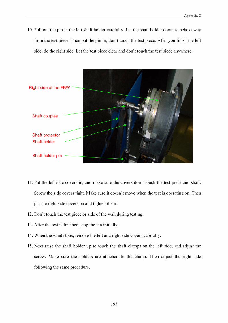
Appendix C
193
10. Pull out the pin in the left shaft holder carefully. Let the shaft holder down 4 inches away
from the test piece. Then put the pin in; don’t touch the test piece. After you finish the left
side, do the right side. Let the test piece clear and don’t touch the test piece anywhere.
11. Put the left side covers in, and make sure the covers don’t touch the test piece and shaft.
Screw the side covers tight. Make sure it doesn’t move when the test is operating on. Then
put the right side covers on and tighten them.
12. Don’t touch the test piece or side of the wall during testing.
13. After the test is finished, stop the fan initially.
14. When the wind stops, remove the left and right side covers carefully.
15. Next raise the shaft holder up to touch the shaft clamps on the left side, and adjust the
screw. Make sure the holders are attached to the clamp. Then adjust the right side
following the same procedure.
Shaft holder Shaft protector
Shaft couples
Right side of the FBW
Shaft holder pin

Appendix C
194
16. One person holds the test piece, and the another person loosens the screws of the left shaft
clamp carefully. Repeat with the right side. When the tops of the shaft clamps have been
removed, hold the test piece and remove it from the force balance.
17. Reinstall the wall covers side by side. Make sure the walls of the force balance are
protected by the covers at all times.

Appendix D
195
Appendix D – Operation manual for force balance (B)
(Test piece inside of the duct)
The operation must keep the force balance safe and force free. When a test piece is working
inside of the duct, attention must be paid to the installation. The following operations must be
completely by two people.
1. The operation must keep the force balance safe and force free. When a test piece is
working inside of the duct, attention must be paid to the installation. The following
operations must be completely by two people.
2. Two people push the force balance near the plexiglass duct. Let the base of the force
balance be close to the edge of the glass duct. Be careful, do not touch the side covers.
3. Then put two pieces of wood of ½ inch thickness under both side balance base. Push the
force balance close to the inside wall (the glass window side) of the tunnel, while making
sure that the shaft is in the centre of the duct. Make sure the test axis of the force balance
is at the same level with the slot of the plexiglass duct. Remove the covers of the walls
carefully, and then put the shaft couples onto the force walls (see the Test Manual for the
Force Balance, when a test piece is working outside of the Duct).
4. Put the lift shaft protectors in, make sure they don’t touch the balance wall and haft
clamps. If required, adjust the screws in the aluminum plate to make sure the shaft
protector doesn’t touch the shaft couple.
5. Next adjust the shaft protectors in the right position compared to the shaft couples. Make
sure the two pieces of shaft protectors are in the same line. This requires two people for
completion.
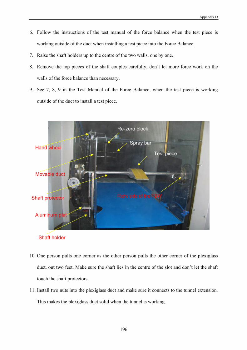
Appendix D
196
6. Follow the instructions of the test manual of the force balance when the test piece is
working outside of the duct when installing a test piece into the Force Balance.
7. Raise the shaft holders up to the centre of the two walls, one by one.
8. Remove the top pieces of the shaft couples carefully, don’t let more force work on the
walls of the force balance than necessary.
9. See 7, 8, 9 in the Test Manual of the Force Balance, when the test piece is working
outside of the duct to install a test piece.
10. One person pulls one corner as the other person pulls the other corner of the plexiglass
duct, out two feet. Make sure the shaft lies in the centre of the slot and don’t let the shaft
touch the shaft protectors.
11. Install two nuts into the plexiglass duct and make sure it connects to the tunnel extension.
This makes the plexiglass duct solid when the tunnel is working.
Shaft holder
Shaft protector
Movable duct
Hand wheel Test piece
Re-zero block
Spray bar
Right side of the FBW
Aluminum plat

Appendix D
197
12. After the test, stop the fan. Unscrew the nuts of the plexiglass duct. Two people at
different sides (left and right) of the duct push the plexiglass duct into the tunnel. Don’t
touch the force balance and test piece, when pushing on the plexiglass duct.
13. Raise the shaft holders up to touch the shaft couples. Lift the left side first and then the
right side. Loosen the screws and remove the test piece with care. This requires two
people to complete this job.
14. Remove the shaft protectors carefully. One person loosens the screws in the aluminum
plate, while the other person holds the protectors.
15. Finally, install the side covers to protect the side walls of the force balance.


![SWEDEN'S BOLD ACTIVITIES IN MEASUREMENTS …...Winterwind 2011 in [1]. Keywords: wind energy, icing, measurements, mapping of icing, de-icing, production losses LEGEND AND ABBREVIATIONS](https://img.dokumen.tips/doc/110x75/5fc882ecda226022c914dc53/swedens-bold-activities-in-measurements-winterwind-2011-in-1-keywords-wind.jpg)