Embed Size (px)
Citation preview

CONVECTION, DIFFUSION AND REACTION:
BRIDGING SCALES IN SCIENCE AND ENGINEERING
A Dissertation presented to the UNIVERSITY OF PORTO
for the degree of Doctor in Chemical and Biological Engineering by
João Pedro Lopes
Supervisor: Prof. Alírio E. Rodrigues, University of Porto
Co-Supervisor: Dr. Silvana S. Cardoso, University of Cambridge
Associate Laboratory LSRE-LCM, Department of Chemical Engineering
Faculty of Engineering, University of Porto
2011

ii
João Pedro Lopes, 2011
Laboratory of Separation and Reaction, Associate Laboratory LSRE/LCM
Department of Chemical Engineering, Faculty of Engineering, University of Porto
Rua Dr. Roberto Frias
4200-465 Porto
Portugal
iii
ABSTRACT
Microchannel reactors are a fundamental building block of chemical reaction engineering. One may find
them in a permeable catalytic material as an idealized geometry for a single pore, in a fabricated
microreactor, or as a cell in a monolith honeycomb. At different scales, all these structures materialize the
concept of process intensification through mass/heat transfer enhancement and/or by miniaturization. The
behavior of these systems is determined by the interplay of convection, diffusion and reaction in the open
channel and surrounding catalyst domains. In this study, we propose an analysis of these interactions,
using scaling and approximate analytical methods. First, we considered the determination of the
conversion of reactant in the problem of mass transfer in channel flow with finite linear wall kinetics, for
different degrees of the concentration profile development. Then, the analysis was extended to the case
where a nonlinear reaction occurs, in the limits of kinetic and mass transfer control. These results were
compared with numerical simulations and found to be in reasonable agreement.
A uniformly valid description concerning the degree of development of the concentration (or temperature)
profile was also pursued. For this purpose, we developed the application of an asymptotic technique to the
series which is the solution of the classical problem. The result can be written as a combination of the
predictions from limiting theories and the intermediate region appears well characterized. The extension
of this transition zone is bounded between the inlet regime length and the distance at which the profile
can be considered fully developed, both given explicitly in terms of the parameters and of an appropriate
criterion which can be set as desired.
Concerning the competition between mass transfer towards the catalyst and reaction at the wall, scaling
analysis suggests that the correct scales for external and internal transport should be included in the
criterion for diffusional limitation. This gives origin to the concept of a rescaled Damköhler number
Da* . These order-of-magnitude predictions are confirmed in more detail by correlations for the degree
of mass transfer control θ . It is proposed that boundaries for kinetic and mass transfer control should be
plotted for specified values of θ in a diagram, with the Damköhler and Graetz’s numbers as axes.
At the scale of the catalyst coating, the internal reaction-diffusion processes were considered and
boundaries between limits derived explicitly in terms of the operating temperature. The relationship with
regimes defined by external phenomena was examined and the dimensionless group which establishes the
overall picture in diffusional limitations at both channel and catalytic coating was identified. An improved
calculation method for the effectiveness factor was proposed, based on a typical geometrical
characteristic of thin coatings. This has found application in the description of nonlinear kinetics, non-
uniform geometries and egg-shell catalyst particles.
The interaction between the same mechanisms appears in the analysis of perfusive catalyst particles and
walls, where intraparticular convection is possible due to the existence of ‘large pores’. We have derived
an expression for the effectiveness factor in a monolith with a permeable wall and shown that the
conditions under which the performance enhancement is maximum correspond to strong convective
transport, but only if this is ‘matched’ by a fast reaction. In a slab-shaped catalyst with a zeroth-order
exothermic reaction, we estimated the effectiveness factor and maximum temperature in a number of
regimes, represented in an operating diagram with axes defined by the intraparticular Peclet number,
Thiele modulus and Lewis number.

iv
v
RESUMO
Um microreactor é um elemento base em engenharia das reacções. Pode ser encontrado num material
catalítico permeável como uma geometria idealizada para um poro, num microreactor fabricado, ou como
uma célula de um monólito. Em escalas diferentes, todas estas estruturas materializam o conceito de
intensificação de processos através da melhoria da transferência de massa/calor e/ou através de
miniaturização. O comportamento deste sistemas é determinado pela interação entre convecção, difusão e
reacção nos domínios do canal e do catalisador circundante. Neste estudo, proposemos uma investigação
destas relações, utilizando análise de escalas e métodos analíticos aproximados. Em primeiro lugar,
considerámos a determinação da conversão de reagente no problema de transferência de massa em
escoamento num canal, com uma reacção de primeira-ordem na parede, para diferentes graus de
desenvolvimento do perfil de concentração. Em seguida, a análise foi alargada ao caso em que uma
reacção não-linear ocorre, nos limites de controlo cinético e difusional. Estes resultados foram
comparados com simulações numéricas e a concordância entre ambos foi considerada razoável.
Uma descrição uniformemente válida no que diz respeito ao grau de desenvolvimento do perfil de
concentração (ou temperatura) também foi procurada. Para atingir esse objectivo, desenvolvemos a
aplicação de uma técnica assimptótica à série que é solução do problema. O resultado pode ser escrito
como uma combinação das teorias clássicas formuladas em limites, e a região intermédia surge bem
caracterizada. A extensão desta zona de transição está limitada entre o comprimento do regime de entrada
e a distância à qual o perfil pode ser considerado perfeitamente desenvolvido, ambos formulados
explicitamente nos parâmetros e num critério apropriado que pode ser estabelecido como desejado.
No que diz respeito à competição entre transferência de massa para o catalisador e reacção na parede, a
análise de escalas sugere que a escala correcta para transporte interno e externo deve ser incluída no
critério para limitações difusionais. Isto dá origem ao conceito de número de Damköhler redimensionado
*Da . Estas previsões são confirmadas por correlações para o grau de controlo diffusional θ . É sugerido
que os limites para controlo cinético e difusional deverão ser representados para valores específicos de θ
num diagrama, com os números de Damköhler e Graetz como eixos.
O processo de reacção-difusão foi considerado à escala da camada catalítica e derivaram-se fronteiras
entre os limites em termos da temperatura de operação. A relação com fenómenos externos foi examinada
e o grupo adimensional que estabele o quadro completo em termos de limitações difusionais foi
identificado. Um método de cálculo melhorado para o factor de eficiência foi proposto, baseando-se na
reduzida espessura dos revestimentos catalíticos. Este procedimento encontrou aplicação na descrição de
cinéticas lineares e não-lineares, geometrias não-uniformes e partículas catalíticas peliculares.
A interação entre os mesmos mecanismos surge na análise de partículas e paredes com poros largos, onde
é possível existir convecção intraparticular. Neste caso, derivámos uma expressão para o factor de
eficiência num monólito com parede permeável e mostrámos que as condições em que o aumento do
desempenho é máximo correspondem a um forte transporte convectivo, mas apenas se este for
acompanhado por uma reacção suficientemente rápida. Num catalisador com geometria de placa plana e
uma reacção exotérmica de ordem zero, estimámos o factor de eficiência e a temperatura máxima em
vários regimes, representados num diagrama de operação que tem como eixos o número de Peclet
intraparticular, o módulo de Thiele e o número de Lewis.

vi

vii
RÉSUMÉ
Un microréacteur est un élément essentiel en ingénierie des réactions. Il peut être trouvé dans un matériau
catalytique perméable comme une géométrie idéalisée pour un pore, dans un microréacteur fabriqué, ou
comme une cellule d'un monolithe. À des échelles différentes, toutes ces structures matérialisent le
concept de l'intensification de procédés en améliorant le transfert de masse/chaleur et/ou grâce à la
miniaturisation. Le comportement de ces systèmes est déterminé par l'interaction entre convection,
diffusion et réaction dans les domaines du canal et du catalyseur avoisinant. Dans cette étude, nous
proposons une analyse des ces interactions en utilisant l'analyse d'échelle et des méthodes analytiques
approximées. Premièrement, nous avons considéré la détermination de la conversion du réactif dans le
problème du transfert de masse en flux dans un canal, avec une réaction de premier ordre sur la paroi,
pour différents degrés de développement du profil de concentration. Ensuite, l'analyse a été étendue au
cas où une réaction non-linéaire se produit, dans les limites du contrôle de la cinétique et difusionnel.
Une description uniformément valable en ce qui concerne le degré de développement du profil de
concentration (ou température) a également été recherchée. Afin d'atteindre cet objectif, nous avons
développé l'application d'une technique asymptotique à la série qui est la solution du problème. Le
résultat peut être écrit comme une combinaison de théories classiques formulées en limites, et la région
intermédiaire apparaît bien caractérisée. L'étendue de cette zone de transition est limitée entre la longueur
du régime à l'entrée et la distance à laquelle le profil peut être considéré comme pleinement développé,
ces deux termes sont explicitement formulés dans les paramètres et dans un critère approprié qui peuvent
être défini comme désiré.
En ce qui concerne la compétition entre le transfert de masse pour le catalyseur et la réaction sur la paroi,
l'analyse d'échelle suggère que l'échelle correcte pour le transport interne et externe doit être inclue dans
le critère pour des limitations diffusionnelles. Cela donne lieu à la notion de nombre de Damkohler
redimensionné *Da . Ces prévisions sont confirmées par corrélations pour le degré de contrôle
diffusionnel θ . Il est suggéré que les limites pour un contrôle cinétique et diffusionnel devront être
représentées pour des valeurs spécifiques de θ dans un diagramme, avec les numéros de Damkohler et
Graetz comme axes.
Le processus de réaction-diffusion a été considéré à l'échelle de la couche catalytique et des frontières
entre les limites en termes de température de fonctionnement en ont dérivé. Une méthode de calcul
amélioré du facteur d'efficacité a été proposée, basée sur l'épaisseur réduite des revêtements catalytiques.
Cette procédure a trouvé une application dans la description de cinétiques linéaires et non linéaires,
géométries non-uniformes et particules catalytiques pelliculaires.
L'interaction entre les mêmes mécanismes apparaît dans l'analyse de particules et parois avec de larges
pores, où il peut y avoir une convection intraparticulaire. Dans ce cas, nous avons dérivé une expression
pour le facteur d'efficacité d'un monolithe avec une paroi perméable et nous avons montré que les
conditions dans lesquelles l'augmentation de performance est maximale correspondent à un fort transport
convectif, mais seulement si celui-ci est accompagné par une réaction suffisamment rapide. Dans un
catalyseur de géométrie de plaque plane et une réaction exothermique d'ordre zéro, nous avons estimé le
facteur d'efficacité et la température maximale dans plusieurs régimes, représentés sur un diagramme
d'opération avec les nombres de Péclet intraparticulaire, Thiele et Lewis comme axes.

viii

ix
ACKNOWLEDGEMENTS
I would like to acknowledge Prof. Alírio Rodrigues for sharing with
me his time and ideas during the supervision of this thesis, but perhaps
more importantly, for generously allowing me to build my own path.
I am equally indebted to Dr. Silvana Cardoso for the valuable
suggestions provided and for welcoming me into her research group
during my visits to the Department of Chemical Engineering and
Biotechnology in Cambridge.
Financial support from Fundação para a Ciência e Tecnologia
(SFRH/BD/36833/2007) is also thankfully acknowledged.
Finally, I would like to express my gratitude to my family and friends
for their understanding, encouragement and genuine affection.

x

xi
CONTENTS
1 OVERVIEW AND RELEVANCE 1
1.1 Operation in the microspace 2
1.1.1 Reactor miniaturization under fixed efficiency 4
1.1.2 Fluid flow and pressure drop 5
1.1.3 Presence of wall-catalyzed reactions 8
1.1.4 Impact on mass transfer 10
1.1.5 Implications on heat transfer 11
1.2 Applications of microchannel reactors 13
1.2.1 Practical realizations of the microchannel reactor concept 14
1.2.2 Examples of applications 15
1.3 Characteristic regimes in microchannel reactors 20
1.3.1 Intrinsic kinetic measurements 21
1.3.2 ‘New’ operating regimes in microprocessing 24
1.4 Transport enhancement in catalytic structures due to intraparticular convection 27
1.4.1 Convection as an additional transport mechanism in ‘large-pore’ materials 27
1.4.2 Modeling of intraparticular convection coupled with reaction in catalyst
particles
29
1.5 Thesis objectives and outline 33
Notation 36
References 38
2 MASS TRANSFER IN A WALL-COATED MICROCHANNEL: FINITE REACTION
RATES & KINETIC NORMALIZATION
49
2.1 Introduction 49
2.2 Graetz-Nusselt regime (dominant transverse diffusion and convection) 51
2.2.1 Theoretical background 55
2.2.2 Approximation to the eigenvalues 57
2.2.3 Approximation to n
w coefficients 60
2.2.4 One-term approximation for the mixing-cup concentration 63
2.3 Lévêque’s regime (dominant convection) 68
2.3.1 Structure of the perturbation problem in Lévêque’s regime 69
2.3.2 Approximate solution to Lévêque’s problem under finite reaction rate conditions
70
xii
2.3.3 Higher order corrections to Lévêque’s problem 73
2.3.4 Effect of curvature in a circular channel with plug flow 74
2.3.5 Effect of nonlinear velocity profile in laminar flows 75
2.4 Kinetic normalization for ‘power-law’ reaction rates 77
2.4.1 Developing concentration profile 78
2.4.2 Fully developed concentration profile 85
2.5 Conclusions 89
Notation 90
References 92
3 BRIDGING THE GAP BETWEEN GRAETZ AND LÉVÊQUE’S THEORIES FOR
MASS/HEAT TRANSFER
97
3.1 Introduction 97
3.2 Instantaneous concentration annulment at the wall (or uniform wall temperature) 102
3.2.1 Asymptotic dependence of eigenvalues and coefficients 102
3.2.2 Structure of the mixing-cup concentration/temperature profile 104
3.2.3 Lévêque’s regime limit 108
3.2.4 One-term Graetz regime limit 109
3.3 Uniform wall mass / heat flux 110
3.3.1 Asymptotic dependence of eigenvalues and coefficients 111
3.3.2 Uniformly valid approximation to Sherwood/Nusselt number 111
3.3.3 Limiting forms of Eq.(3.35) 115
3.4 Transition criteria between regimes and ranges of validity 115
3.4.1 Dirichlet boundary condition 116
3.4.2 Neumann boundary condition 119
3.4.3 Comparison with previous criteria 122
3.5 Finite linear wall kinetics 125
3.5.1 Assumptions on the dependence of eigenvalues and coefficients 125
3.5.2 Contributions to the mixing-cup concentration profile 127
3.5.3 Calculation procedure for the conversion profile 136
3.5.4 Developing length of the concentration profile 138
3.5.5 Other cross-sectional geometries 140
3.6 Conclusions 141
Notation 141
References 143
xiii
4 CRITERIA FOR KINETIC AND MASS TRANSFER CONTROL IN A WALL-COATED
MICROREACTOR
147
4.1 Introduction 147
4.2 Scaling and operating regimes definition 149
4.2.1 Global scale regimes 149
4.2.2 Local scale regimes 151
4.2.3 Interphase mass transport - wall reaction regimes 152
4.3 Degree of external mass transport limitation 154
4.3.1 Fully developed concentration profile 154
4.3.2 Developing concentration profile 158
4.3.3 Iso-θ curves in the m
Da Pe zα− diagram 160
4.4 Comparison with previous criteria in the literature 163
4.5 Inlet effects 169
4.5.1 Local (inner) scaling in the axial and radial directions 169
4.5.2 Rescaled Damköhler number for inlet effects 172
4.6 Conclusions 177
Notation 178
References 179
5 EFFECTIVENESS FACTOR FOR THIN CATALYTIC COATINGS 183
5.1 Introduction 183
5.2 Problem formulation 187
5.2.1 One-dimensional cylindrical model for a catalytic coating 187
5.2.2 Effectiveness factor 190
5.3 Perturbation solution for thin catalytic coatings 190
5.3.1 Linear kinetics 191
5.3.2 Nonlinear kinetics 192
5.3.3 Egg-shell catalysts 197
5.4 Uniform annular coating 199
5.4.1 Linear kinetics 201
5.4.2 Nonlinear kinetics 203
5.5 Nonuniform coatings 205
5.5.1 Circular channel in square geometry 205
5.5.2 Square channel with rounded corners 207
xiv
5.6 Interplay between internal and external mass transfer – reaction regimes 208
5.6.1 Kinetic regime 210
5.6.2 Diffusional regime 216
5.6.3 Mapping of operating regimes 219
5.7 Perfusive catalytic coatings and monoliths 222
5.7.1 Model equations for a perfusive hollow cylinder 225
5.7.2 Perturbation solution for specified surface concentration and pressure
profiles
227
5.7.3 Performance enhancement 231
5.8 Conclusions 234
Notation 236
References 237
6 NONISOTHERMAL EFFECTS IN PERFUSIVE CATALYST PARTICLES 245
6.1 Introduction 247
6.2 Operating regimes 247
6.2.1 Governing equations and model parameters 247
6.2.2 Scaling and regime diagram 250
6.3 Perturbation analysis 257
6.3.1 Regime I (Chemical regime) 258
6.3.2 Regime II (Diffusional regime) 262
6.3.3 Regime III (Strong intraparticular convection regime) 272
6.4 Maximum temperature estimate 278
6.5 Effectiveness factor approximation 280
6.6 Conclusions 281
Notation 283
References 285
7 CONCLUSIONS AND PERSPECTIVES OF FUTURE WORK 289

1
CHAPTER
ONE
OVERVIEW AND RELEVANCE
1
Convection, diffusion and reaction are simultaneously present in several chemical engineering
phenomena. A well-defined interaction of these mechanisms at several scales is key for the
development of strategies for process intensification. Microreaction technology has emerged as
one of those strategies, or more generically as a new paradigm for the chemical industry aiming
improved performance. One of the main objectives of this thesis is to provide an analysis of the
transport-reaction problem in a wall-coated microchannel using approximate analytical
techniques. In this chapter, we review the driving forces for miniaturization which can be
explained in terms of the length scales governing each transfer mechanism (section 1.1). Then,
the practical motivation behind microprocess engineering is briefly illustrated with examples of
applications in different fields (section 1.2).
Our analysis also includes the definition of characteristic regimes, which is a topic of great
interest in the design and operation of microdevices. Actually, conceptual development of a
provess involves several stages in different regimes and a comprehensive description is
required. Moreover, microreactors are known for opening new opportunities in parameter
spaces which are unfamiliar to the conventional technologies. Some studies which are typically
conducted in a widespread range of conditions are detailed in section 1.3.
Process intensification in the sense of enhancement of mass/heat transfer rates can also be
accomplished by means of another concept: the promotion of convective transport, where
conventionally only diffusion existed to assure transport. This can be implemented in both
microreactors with permeable walls and catalyst particles. A review concerning the effect of this
additional mechanism inside catalytic structures is presented in section 1.4. Finally, the outline
of the thesis is described in detail, along with the specific objectives and methods employed in
each chapter (section 1.5).

CHAPTER 1
2
1.1 OPERATION IN THE MICROSPACE
The ‘microspace’ results from the reduction of the characteristic dimensions and its implications
on flow, mass and heat transfer, coupled with eventual homogeneous and heterogeneous (wall-
catalyzed) reactions. The terms ‘characteristic length’ or ‘length scale’ refer to the distance over
which an appreciable change in a quantity of interest occurs (e.g. changes in velocity,
temperature or concentration). In fact, microdevices are composed by structures whose
dimensions are of the order of several tens to hundreds of micrometers. As a result they exhibit
high surface to volume ratios. If the characteristic geometrical distance is a , then
1~surf
S
V a. (1.1)
Values of this ratio have been reported to be around 10 000 to 50 000 m2/m3 (Ehrfeld et al.
2000), which are much larger than the ones for convectional technologies (1 – 10 m2/m3). The
natural geometry to consider is a channel, and in particular the single channel design is
attractive, either as a model for multichannel configurations or as a technology on its own for
laboratory and small scale production, with manageable investment costs, safety concerns and
control effort. However, apart from specific applications where a precise control of harsh
conditions is expensive, parallelization or numbering up is always a possible strategy to increase
the productivity.
A consequence of (1.1) is the decrease of the characteristic times for heat / mass transfer and
mixing, i.e. enhancement of transport processes. Therefore, microtechnology offers
opportunities for process intensification from several perspectives (Charpentier 2005; Becht et
al. 2007; Becht et al. 2009; Van Gerven et al. 2009): pure reduction in plant size, increase in
selectivity with reduction of waste by rigorous control of residence time and temperature
gradients, and maximization of the interfacial area to which driving forces are applied. The
timescales for several processes and their dependence on the geometrical characteristics of a
microchannel are listed in Table 1.1. If these quantities are combined in the form of ratios, then
several dimensionless parameters arise. It is possible to observe that different dependencies are
present: second-order (diffusive) processes are more significantly affected from reduction in a .
The process with the longest timescale will be controlling, and the design of the microgeometry
should take this into consideration.
An analysis based on these time constants for transport phenomena and reactive processes
allows one to identify the operations that benefit the most from miniaturization and to compare
them with processes occurring at the conventional scale. Many reviews exist in the literature
concerning the effect of scaling down. In particular, we highlight the case where a wall-
catalyzed reaction occurs in a coated microchannel.

OVERVIEW AND RELEVANCE
3
Table 1.1: List of characteristic times for transport-reaction processes
Process X Timescale, X
τ
Convection (flow) L
u ~ L
Viscous diffusion
2a
ν
2~ a
Transverse mass diffusion / heat conduction 2
a
D;
2a
κ 2~ a
Axial fluid mass diffusion / heat conduction 2
L
D;
2L
κ 2~ L
Interphase mass / heat transfer
(fully developed profile: , constantNu Sh = )
2
~surf
m
V S a
k Sh D;
2
~surf
heat
V S a
k Nu κ 2~ a
Interphase mass / heat transfer
(developing profile*: 1, ~Nu Sh δ− )
2
~surf
m
V S a
k D
δ;
2
~surf
heat
V S a
k
δ
κ 2~ a δ
Reaction (ref. coating volume) ( )
10 0
0
mc c
c k
−
=R
Homogeneous reaction ( )
10 0
0
m
bulk bulk
c c
c k
−
=R
Wall-catalyzed reaction
(no internal diffusion limitations)
1 10 0~
m m
surf surf surf
c V c a
k S k
− −
~ a
Heterogeneous reaction in coating
(internal diffusion limitations**) ( )
10 0
0
~m
obs surf
c a c
c k η
−
R ~ a
Heat generation by chemical reaction ( ) ( ) ( )
, 00 0
0 0
P fluid
ad R
C TT c
T c H c
ρ=
∆ −∆R R
Heat removal by wall conduction (transverse) 2w
wall
t
κ
Reactor heat-up ,
,
wall P wall wall
P fluid
C V
m C
ρ
ɺ
Notes: a and L are the characteristic dimensions in the transverse and axial directions, respectively; for
the remaining nomenclature please refer to the Notation section at the end of the chapter; *details on the
scale for transport under developing profile conditions ( ~ δ ) can be found in Chapters 2 and 4; **details
concerning the use of the effectiveness factor (η ) can be found in Chapters 4 and 5; ( )0cR is expressed
as a power-law kinetics in some expressions ( 0m
k c ); w
t is the thickness of the catalytic body.

CHAPTER 1
4
1.1.1 Reactor miniaturization under fixed efficiency
A simple methodology for the design of microreactors, comparison with conventional
technologies and identification of the most interesting operations was developed by Commenge
et al. (2005). Since in large part this is based on the analysis of the timescales given in Table
1.1, we now summarize the main aspects of this work.
These authors consider reduction of reactor volume (and of the characteristic distance for
transfer processes), while keeping efficiency fixed for hydrodynamic and chemically equivalent
systems. This naturally requires the definition of both process efficiency and equivalence
criteria. According to Commenge et al. (2005), a microstructured reactor is ‘equivalent’ to a
fixed bed packed with nonporous spherical catalyst particles if they present the same porosity,
surface area to volume ratio and space time,
bed microε ε= ,
surf surfbed micro
V V
S S
=
and
bed microτ τ= . (1.2)
This implies that the cross-sections, heights, catalyst amounts and feed flowrates feed
Q of both
reactors are the same, and that the particle diameter in the fixed bed is related to the diameter of
a cylindrical channel by
13
2micro
part channel
micro
d dε
ε
−= . (1.3)
Since the spherical particles are only active at the surface, they observe that the two systems
related by Eqs.(1.2) and (1.3) present the same conversion for a large range of parameters. In
either case, the efficiency is defined as the ratio of two characteristic times, the space time of the
process fluid in the system and the one for the operation being considered controlling,
conv
X
NTUτ
τ= , (1.4)
where conv
L uτ = and X
τ is given in Table 1.1 for some common processes. As long as the
number of transfer units ( NTU ) remains constant, the performance is fixed regardless of the
scale. Therefore, systems with different dimensions can be compared on the same basis.
For this discussion, the timescales for transport and reaction mechanisms can be grouped in
terms of their dependence on the channel characteristic distance a . Then, the implications of
reducing a on the reactor volume and pressure drop are examined (Hessel et al. 2004;
Commenge et al. 2005; Renken et al. 2008). We write the microstructured reactor volume and
pressure drop as
( ) ~reactor ch ch X feed X
V N A L NTU Qτ τ= = (1.5a)
OVERVIEW AND RELEVANCE
5
2 2
4 4 2~ ~ ~feed ch
ch ch X ch X ch
Q L A L LP
N d d NTU dτ τ∆ (1.5b)
since NTU and ~feed ch ch X
Q N A L τ are constant (independent from channel dimensions).
Control by processes with high order dependences on a , leads to the most expressive reduction
of reactor volume with the decrease of the length scale. On the other hand, pressure drop
increases unless 4~ch
N L a− , which according to Eq.(1.5a) leads to 2 2~
reactorV a L
− (which
decreases as X
τ with a if ~X
L a τ ). For example, if mass transfer towards the coating phase
is controlling:
• the reactor volume decreases with a as 2~reactor
V a
• the dependence of pressure drop on a is 2
4~
LP
a∆
• miniaturization does not result in a pressure drop increase if 2~L a and 2~ch
N a− .
Note that here the symbol ~ is used with the meaning “increases/decreases with decrease of a
as”. Therefore, 2~L a means that if a is reduced from 1 mm to 100 µm , L should be reduced
from 1 m to 1 cm. This simplified analysis is only possible when there is a clearly controlling
mechanism. In general, several effects may appear at leading-order behavior and further
assumptions are required. However even for more idealized situations, the design equations
need to be written with the correct coefficients and are more complicated than simple scaling
rules. Thus, the analysis of regimes which consider the interplay e.g. between mass transfer and
reaction are interesting to complement this approach (see Chapters 2 and 3 of this thesis). The
definition of the areas where one mechanism is clearly controlling is also of interest (see
Chapters 3 and 4 of this thesis). In the same line, Renken et al. (2008) proposed design rules
obtained from comparison of the residence time in a microreactor with the time constants for
several controlling processes. Note that the system’s conversion (and therefore specific
productivity) is related with NTU . We now briefly review the implications of scale down in
fluid flow, energy consumption, heat and mass transfer, in the absence or presence of chemical
reactions in microchannels.
1.1.2 Fluid flow and pressure drop
A major simplification in the modeling of microchannels is to assume a well-defined velocity
profile, decoupling fluid mechanics from the problem. Namely, laminar flow is likely to be
found since the timescale for viscous diffusion is much smaller than the one for convection, i.e.
from Table 1.1:

CHAPTER 1
6
2
1a
a uRe
Lα
ν= << , (1.6)
where the two dimensionless parameters are the aspect ratio ( a Lα = ), which is typically
small; and the Reynolds number (a
Re a u ν= ), which is commonly in the laminar range for
channel flow. This allows the problem to be treated analytically and the solutions presented in
this thesis will rely on this assumption. The effect of simultaneous development of the velocity
profile compared with concentration/temperature fields requires numerical evaluation and the
importance of this is measured by Prandtl’s number for heat transfer or by Schmidt’s number
for mass transfer:
Prν
κ= and Sc
D
ν= . (1.7)
When Pr → ∞ and Sc → ∞ , the flow field develops much faster than the concentration or
temperature profiles. In the opposing limit ( 0Pr → and 0Sc → ), ‘plug-flow’ can be used as an
idealized inlet profile. Solutions obtained for both cases will be presented in Chapters 2, 3 and
4, in the perspective of lower and upper bounds. The entrance length before which the velocity
profile can be considered developed is often given by an expression of the type (Bird et al.
2002)
~ 0.14e
a
LRe
a, (1.8)
here written for flow in a circular channel. There is a similarity between the entrance length of
velocity and concentration/temperature profiles. In Chapter 3, the thickness of this region is
discussed for the mass/heat transfer problem.
The pressure drop is important to quantify the process energy requirements and sometimes even
limiting of the design and performance of a microdevice. It is related to the friction factor by
(Bird et al. 2002)
2
2h
uLP f
d
ρ∆ = (1.9)
The (Darcy’s) friction factor f in a straight channel is inversely proportional to the Reynolds
number ReD h
u d ν= , according to
Ref
D
Cf = , (1.10)
where for fully developed velocity profile, the coefficient f
C can be found for several cross-
sectional shapes (Shah et al. 1978) (it equals 64 in a circular channel and 96 in a planar
channel).
OVERVIEW AND RELEVANCE
7
1.1.2.a Pressure drop reduction
A significant advantage in the adoption of microreaction technology would be the reduction in
energy consumption. It is known that up to a certain extent, this is related to the pressure drop in
the system. For ‘equivalent’ microstructured and packed bed configurations (in the sense
detailed in section 1.1.1), the pressure drop from Poiseuille equation for the former is compared
with Carman-Kozeney equation for the latter to yield (Commenge et al. 2005),
( )
( ) 2bed k
ch
P L h
P Lµ
∆=
∆. (1.11)
Eq.(1.11) is the ratio between the mean length of passages between particles and the length of a
straight capillary tube, given by 2k
h . Since ~ 4.5 5k
h − , the pressure drop can be reduced up to
2.5 times in a microreactor.
1.1.2.b Scaling effects
A question that always arises when discussing flow in microchannels, and particularly
microflows, is the validity of the continuum theory. The extent of these deviations is assessed
by the magnitude of the Knudsen number
mean
charact
Kn =ℓ
ℓ, (1.12)
and their implications range from wall slip in gas flows to more unclear consequences in liquid
flows. The literature presents contradictory conclusions concerning the need to account for these
‘new’ effects. Doubts related with the accuracy of experimental measurements at small scales
with ‘large’ analysis equipment (Hessel et al. 2004) contribute to the assumption of continuum
behavior for (Bruus 2008; Herwig 2008)
310Kn−
< (gas flows)
and liquid flows with ,~ 10mean gasℓ . For mean free path for gases ~ 50 nm
meanℓ , this implies
50 µmcharact ch
d= >ℓ . Since the diameter of the channel at such small scales will be fixed by
fabrication and cost limitations, if ch
d is between 100 µm and 500 µm , then the continuum
approach is valid (Mills et al. 2007). In tubes with diameters below 150 µm , some deviations of
the product of the friction factor and Reynolds number from theoretical values were explained
by the failure in accounting for surface roughness (Judy et al. 2002). Other sources of error have
been identified (Pfund et al. 2000). A discussion on the importance of effects such as viscous
dissipation and the appropriate simplifications of the Navier-Stokes equations at the microscale
can be found elsewhere (Herwig 2008).

CHAPTER 1
8
1.1.3 Presence of wall-catalyzed reactions
Heterogeneous reactions occurring at the microchannel wall or in a catalytic coating attached to
this surface are of particular interest due to the large values of the surface to volume ratio,
Eq.(1.1). This is in agreement with the generic statement that effects referred to the surface are
privileged compared to the ones referred to volume. The dependence of the timescales for these
reactions on the channel diameter compared with their homogeneous counterpart (Table 1.1),
indicate that benefit from miniaturization does not occur if the controlling timescale is the one
for bulk reaction. Actually, there may be a change in mechanism at the microscale and it is
possible that a homogeneous reaction becomes heterogeneous. Moreover, uncoated walls
(stainless steel, iron,…) can act as catalyst for partial or total combustion (Mills et al. 2007).
Therefore, wall catalyzed reactions are of particular interest and their presence introduces
additional design considerations which interact with pressure drop, heat and mass transfer.
1.1.3.a Reactor requirements at the microscale and criteria for miniaturization
The ideal set of conditions for an industrial reactor to be feasible is well-known (Wörz et al.
2001a; Wörz et al. 2001b). Our expectation is that by reducing the characteristic length scale,
some of these requirements are achieved more efficiently or are simply made possible to attain.
This is summarized in Table 1.2. It is commonly accepted that the potential of microdevices
should be focused towards applications where dramatic improvements result, since the
technology is not obviously free of disadvantages and has to compete with already well-
established processes, which benefit from the economy of scale. Concerning the nature of the
reaction, several authors propose that the main candidates to microprocessing should have the
following characteristics:
• fast kinetics;
• exothermic (endothermic) with reasonable (large) reaction heats;
• high temperature;
• complex;
• multiphase;
• hazardous;
• for which conventional technology does not exist or is limited.
Actually, microreactor arrangements may constitute a solution for reactions with a wide range
of characteristics. Roberge et al. (2005) classified reactions in three main types according to
kinetics, and proposed some examples of how microtechnology can answer the challenges

OVERVIEW AND RELEVANCE
9
raised by each one (we have collected this information in Table 1.3). Examples of
microprocesses for applications fulfilling these requirements are presented in section 1.2.
Table 1.2: Fulfillment of ideal requirements by microstructured reactors.
Requirement Purpose Advantages offered by microspace operation
Residence time
needed for reaction
• Attain desired levels of
conversion
• Selectivity
• Exact control of residence time (minimum
backmixing; uniform RTD);
• In particular, very short residence times can
be achieved;
• Transport rates can be matched with kinetics
Efficient heat
removal/supply
• Safety (thermal
runaway, explosive);
• Hot spots reduce
selectivity
• Simultaneous micro heat-exchangers;
• Large surface to volume ratio, enhanced heat
transfer
• Selection of wall material and geometry
(additional design parameter)
Sufficiently large
interface (multiphase
systems)
• Improve contact
between phases and
interphase transport
• large surface to volume ratio in wall-coated
systems
Table 1.3: Reaction classification according to Roberge et al. (2005) and respective
microreaction engineering approach.
Group Reaction characteristics Microtechnology solution
A
• Mixing-controlled
• Rapid kinetics
• Considerable heat release
Multi-injection principle to spread the
reaction over a larger reactor channel length
or heat transfer area (Roberge et al. 2008)
B
• Kinetically controlled
• Slow (reaction time of few minutes)
• Require larger residence times with
appropriate temperature control
Flexible, modular reactor for reaction with
considerable heat release
C • Hazardous or autocatalytic nature
Small volume systems with excellent
temperature control, allowing start under
harsh conditions but safe operation

CHAPTER 1
10
1.1.3.b Matching transfer rates with kinetics for design
It is commonly accepted that microreactors should be designed so that mass and heat transfer
are fast enough compared to the reaction kinetics. A simple comparison of timescales allows the
definition of regions of interest, although a more detailed analysis is required for rigorous
design (see e.g. Chapter 2 of this thesis). Hessel et al. (2004) and Commenge et al. (2005)
suggest that the dimensioning of the channel diameter should be ruled by these considerations.
As can be seen from Table 1.1, heat and mass transfer depend on the channel’s diameter as
2~ch
d , while the time constant for an heterogeneous reaction may be proportional to ~ch
d . For
selected values of ch
d , mass transfer
τ and heat transfer reaction
τ τ< . However, it is recognized that other
factors may limit the possible designs, namely: pressure drop, occurrence of clogging/fouling,
and uniform distribution of flow entering the microchannels. The first two factors suggest the
use of larger diameters, which are also easier to clean (important for pharmaceutical production)
and allow high flow rates. For higher throughputs, the ‘numbering up’ strategy can be used.
Herwig (2008) presented a length-time scales plot comparing mixing by molecular diffusion in
gases and liquids and the characteristic times for slow and fast homogeneous reactions.
We note that even though it appeared from section 1.1.1 that controlling homogeneous reactions
would take no advantage from miniaturization, the fact that ‘new’ conditions can be applied
allows the performance of these processes to be enhanced as well (see sections 1.2.2 and 1.3.2).
1.1.4 Impact on mass transfer
In the case of microdevices operating in laminar flow, transverse mixing is assured only by
molecular diffusion, which as shown in Table 1.1 has a characteristic time proportional to the
square of the channel’s radius or diameter. Jensen (2001) reports that studies with acid-base
reactions show that complete mixing in a liquid-phase microreactor with channels 50-400 µm
wide occurred in 10 ms. Thus, faster mixing implies channel diameter reduction. This also leads
to the increase in pressure drop and a flowrate limitation may appear. This can be surpassed by
numbering up, even though other issues such as uniform fluid distribution arise. Therefore,
several strategies to improve mixing in microchannel apparatus and networks have been
proposed (Hessel et al. 2005b; Falk et al. 2010). The objective is to overcome the limitations in
conventional methods, regarding energy consumption, technical feasibility and detrimental
effect in the process performance (due to backmixing and axial dispersion).
For the design of a single channel microreactor, the control of the residence time is important
for selectivity issues. In preliminary design methods (Hessel et al. 2004; Commenge et al. 2005)

OVERVIEW AND RELEVANCE
11
it is proposed that once the required residence time is fixed, the fluid velocity should selected so
that minimum dispersion is obtained. It is possible however that excessive pressure drop results
from this and a trade-off must be searched.
To highlight the benefits from microstructuring in reducing dispersion, ‘equivalent’ fixed bed
and microreactor (as defined in section 1.1.1) are compared in terms of a dispersion ratio (ratio
of the widths of initially delta-like concentration tracers at the reactor exit) (Hessel et al. 2004;
Commenge et al. 2005; Renken et al. 2008). In terms of the Peclet number (with ax
D as the
axial dispersion), an expression for fixed bed reactor of the type
( ),p
ax
u dPe f Re Sc
D= =
is considered, while for the microchannel the classical Taylor-Aris theory applies (Taylor 1953;
Taylor 1954; Aris 1956). For 3 100u d D< < , Commenge et al. (2005) observed that the
dispersion in a microchannel is smaller than that of a fixed bed reactor with porosity 0.4. These
boundaries change for other values of porosity (the range gets broader for smaller porosities,
and narrower for higher porosities). The minimum dispersion is attained at ~ 14ch
u d D and
corresponds to a 40% reduction in dispersion in a microchannel reactor compared to a fixed-bed
one.
1.1.5 Implications on heat transfer
Perhaps one of the most important consequences from miniaturization is the enhancement and
control of heat transfer rates in both reactive and nonreactive cases. As in the case of mass
transfer, higher heat transport rates are possible due to the high values predicted from Eq.(1.1).
Very high values of heat transfer coefficient are commonly reported for microgeometries and
this has been known for many years (e.g. in the field of electronic microdevices cooling). It is
possible to achieve heat transfer coefficients one order of magnitude higher than in conventional
heat exchangers (Ehrfeld et al. 2000; Mills et al. 2007).
Concerning the validity of macroscale theory in channels with reduced dimensions, Rosa et al.
(2009) provided a critical review, evaluating the importance of scaling effects in single-phase
heat transfer in microchannels. They concluded that even though inconsistencies in published
results exist, the same theory and correlations are applicable as long as ‘scaling effects’ are
explicitly accounted for or can be safely ignored. These ‘scaling effects’ included entrance
effects, conjugate heat transfer, viscous heating, etc., and although they are likely to be ignored
in macro-channels, they now may have a significant influence in heat transfer. They also stress
the role of measurement and fabrication uncertainties and the need for reliable experimental

CHAPTER 1
12
data. Results from single channel designs were found to agree with published correlations better
than multichannel configurations and this was attributed to flow maldistribution, 3-dimensional
conjugate heat transfer and measurements uncertainties. They expect sub-continuum models to
become more important, however probably only relevant at the nano-scale. In particular, these
authors review a number of experimental studies in the literature and conclude that in all of
them entrance effects need to be accounted for. Conclusions in the same direction are taken in
an experimental study from Lee et al. (2005). They assessed a number of classical correlations
to describe thermally developing heat transfer in rectangular microchannels with hydraulic
diameters ranging from 318 and 903 µm and concluded that these were in good agreement, as
long as inlet and boundary conditions are correctly considered. In Chapter 3, we discuss the
relevance and extent of inlet effects in the temperature profile.
A major improvement brought by microprocess technology results from combining superior
heat transfer capabilities with highly exothermic (endothermic) reactions. Kockmann et al.
(2009) discusses heat transfer in microstructures in terms of a volumetric heat transfer
coefficient defined as
ref
V heat
int int
SQU k
V T V= =
∆
ɺ
, (units of W/m3K)
where int
V is the internal volume, ref
S the area of the reference surface and heat
k the heat
transfer coefficient (per interface area). Kockmann et al. (2009) report a study from Kinzl which
gives a threshold for V
U in microreactors with residence time of 10 s and highly exothermic
reactions, so that a mean temperature difference of less than 10 K exists:
( )31 MW m K
VU ≥ .
Then, they estimate that under typical conditions for organic liquids,
( )( )
30.002MW m K
V
ch
Ud m
= ,
which is greater than 1 for 2 mmch
d < . Therefore, microreactors are also heat exchangers and
isothermal operation even for highly exothermic reactions is possible, due to efficient heat
removal/supply. As discussed previously, this opens possibilities for dealing with reactions
releasing large amounts of heat or with risk of explosion. It also improves selectivity of many
processes, due to the reduction or even elimination of hot-spots. Consequently, more aggressive
conditions may be employed (see section 1.3.2).
The fastest mechanism for heat removal is by conduction through the walls, as can be seen from
the timescale in Table 1.1. Therefore, the channel walls can be designed so that due to its
reduced thickness and high-conductivity construction material, no appreciable temperature
gradients are registered. In fact, this provides an additional source for control of temperature and

OVERVIEW AND RELEVANCE
13
heat supply/removal. Ehrfeld et al. (2000) and Hessel et al. (2004) report several examples of
microsystems for carrying out reactions, which are integrated with heat exchangers. This can
happen by adjacent heating/cooling gas channels placed in alternating layers with the process
channels. Due to the low thermal mass of the thin wall, the thermal response is usually fast
(Jensen 2001). Lomel et al. (2006) wrote the characteristic time in both semi-batch and
continuous processes for Grignard reaction as a function of the limiting heat transfer timescale.
They explained the drastic reduction in operation times as being due to the shorter dimensions
of the continuous microprocess, leading to intensified heat transfer and therefore shorter process
times. Hardt et al. (2003) explored microstructuring techniques to enhance heat transfer in
microdevices by at least one order of magnitude (Nusselt numbers as high as 100 were
observed). The performance of the system was also tested in the presence of an endothermic,
heterogeneous, gas-phase reaction. When compared to a conventional fixed bed, reduction in
the amount of catalyst required and overall equipment size was achieved.
Another direction which takes advantage from excellent thermal behavior is the safe realization
of reactions which would result in explosion at the macroscale. Hessel et al. (2004) identified
the key features in microchannel reactor which reduce the risk or prevent the occurrence of
explosions due to chain reactions or to a large heat release. While molecule collisions with the
channel walls may suppress the former, efficient heat transfer is capable of managing the latter.
Two timescales that influence the increase in temperature due to a first-order homogeneous
exothermic chemical reaction are (Table 1.1):
( ) ( )
,~ P fluid wallwall
generation rxn
ad R wall
C TT
T H k T
ρτ τ =
∆ −∆ (1.13)
~ ch
removal
heat
d
kτ .
Eq.(1.13) is usually replaced simply by rxn
τ and is evaluated here at the wall temperature.
Insufficient heat removal or strong heat generation occurs whenever removal generation
τ τ>> , and the
maximum temperature difference approaches the adiabatic limit. Nearly isothermal behavior is
observed in the reverse case, which is favored by the use of smaller channels.
1.2 APPLICATIONS OF MICROCHANNEL REACTORS
The literature is abundant in applications and proofs of concept of technologies employing
microchannel reactors. In fact, several patents have been filled (Hessel et al. 2008a) and some
industrial applications were already reported (Hessel et al. 2005b). At the single channel level,
several new laboratory or small production scale studies appear on a daily basis. As we will

CHAPTER 1
14
discuss, the microchannel reactor concept also describes more consolidated technologies, such
as monoliths. In this case, there are also many review articles (Hoebink et al. 1998; Nijhuis et al.
2001; Kreutzer et al. 2005; Moulijn et al. 2005; Kreutzer et al. 2006) and dedicated monographs
(e.g. Cybulski et al. (1998)).
1.2.1 Practical realizations of the microchannel reactor concept
The description of a system including a channel with the ability to carry reactions due to
catalytic activity at its walls is sufficiently general to encompass a series of technologies. In
fact, this is an idealized portrait that can act as a fundamental model of several practical
solutions in chemical reaction engineering. We however will focus on two approaches in the
field of structured reactors: monoliths and microfabricated channels. Usually, both are
distinguished by different ranges of characteristic dimensions, being monoliths associated with
larger cell hydraulic diameters ( ~ 0.5 1 mmch
d − ). Nevertheless, in terms of mass/heat transfer
intensification with low pressure drops, both technologies claim the same advantages and
sometimes the terms are used interchangeably. However, typically the term ‘monolith’ refers to
a honeycomb arrangement composed by several repeating cells, divided by a ceramic or
metallic material, e.g. Kolaczkowski (1999) and Chen et al. (2008b). It can be pictured as a
catalyst block with a large number of parallel straight channels through which gas flows. On the
other hand, microfabricated reactors are typically generated by precision techniques e.g. on a
metallic plate. A number of fabrication methods (lithography, machining, micro milling, etc.) is
available and details can be found e.g. in Mills et al. (2007) and Ehrfeld et al. (2000). This
distinction may pose significant differences in terms of the channel-channel interaction.
The incorporation of catalyst in the walls of these channels also shares similar characteristics.
This happens in the case where a high surface area washcoat (e.g. γ-alumina) containing the
dispersed catalyst(s) is used, so that sufficient loading is achieved. There are currently a number
of techniques available to coat a microchannel with a catalyst layer (wet impregnation, physical
and chemical vapor deposition, anodic oxidation, sol-gel, slurry and aerosol techniques) and
suitable reviews have been published on the subject (Wunsch et al. 2002; Hessel et al. 2005b).
In the case of the monolith, the wall itself may already contain the catalyst as an integral part of
its structure. In this case, the boundary conditions are more complex and channel interaction in
specific arrangements has to be considered. Problems in microchannel coating are also common
to both cases. Rebrov et al. (2009) identified the reproducible preparation of the catalytic
coating as a crucial requirement in the fabrication of multi-phase microfluidic devices. Besides
reproducibility, other requirements are: homogeneous distribution, mechanical and chemical
stability, and sufficient activity to achieve the desired yield under given conditions. The

OVERVIEW AND RELEVANCE
15
replacement of the catalyst can also become an arduous task. There is also the possibility of a
micropacked bed or a packed monolith. This however typically leads to nonuniform
temperature, concentration and flow profiles (leading to increased pressure drop, channeling and
favoring the appearance of hot-spots), and are more prone to clog. The step of packing the
microchannel also raises some technical issues that require additional study (van Herk et al.
2009). Finally, we refer to another distinction between the two technologies: fabricated
microsystems may include other components, such as micromixers, micro-heat exchangers,
sensors and controllers (Jensen 2001; McMullen et al. 2010).
1.2.2 Examples of applications
According to the characteristics listed above (section 1.1), we can expect a wide range of
reactions to take significant advantages from scaling down. Actually, in the gas-phase, most of
them fulfill all the desired features. For example, partial oxidations are typically highly
exothermic reactions that required solid catalysts. Selectivity is a major issue, as strong
exothermic total oxidation is undesirable. Implementation of more intense conditions is not
feasible in conventional technologies due to difficulties in heat management (Becht et al. 2007).
In this case, microstructured reactors offer the possibility of enhanced control of residence time
and temperature, avoiding hot-spots that harm selectivity and catalyst lifetime.
Several reviews concerning chemicals production on microreactors are available. Srinivasan et
al. (1997) discussed ammonia oxidation in an integrated microreactor. Ehrfeld et al. (2000)
detailed several examples of studies in gas-phase microreactors. Mills et al. (2007) refer some
integrated microreactors for pharmaceuticals manufacture, chemicals production and energy
generation. Kockmann et al. (2009) presents some examples of nitrations and organometallic
reactions, based on Lonza’s industrial experience. Kolb et al. (2007) presents a review of
microreactor for gas-phase selective oxidations. Microreactors for preferential oxidation as a gas
purification step for fuel cells were also addressed. Other examples can also be found in Kolb et
al. (2004), Hessel et al. (2004) and Gokhale et al. (2005). Pennemann et al. (2004) provide a
comparison between microreactor and batch reactor (also stirred vessels and fixed bed reactors
in some cases) for a large number of industrially relevant organic reactions with data taken from
the literature. Their review was divided in ‘small-scale applications’ (e.g. peptide synthesis,
aldol reactions, hydrogenations, dehydrations) and ‘lab / pilot scale syntheses’ (e.g. nitrations,
organomethalic reactions, oxidations, hydrogenations, chlorination and fluorination). This
referred to fine chemicals applications with flow rates up to several milliliters per hour and from
that to several tens of liters per hour, respectively. While the main concern at the small-scale
appears to be conversion (which generally register improvements in microreactors), at larger

CHAPTER 1
16
scales increase in the process yield and selectivity is also desired (and this is also visible in the
results from microdevices). From these examples, it is possible to observe two other important
facts: in some cases, the reaction conditions change dramatically (temperature increases from
cryogenic to more reasonable values) and the residence times are drastically reduced (from
several hours/days to seconds). Mae (2007) gives several examples of organic syntheses in
microreactors highlighting the following advantages: shortening of reaction time, solvent-free
operation, new synthesis routes, control of unstable intermediates, severe conditions, safe
operation under explosive / thermal runaway conditions, and omission of catalysts and reagents.
Other examples are given in McMullen et al. (2010). Each case presents particular challenges
that microtechnology may solve completely or at least minor its adverse effects. Summary of
some particular cases can be found in Table 1.4.
Application of microprocessing in the field of energy generation has gained particular interest
and is nowadays a major line of research in the production of purified hydrogen for fuel cells
and portable aplications (Kundu et al. 2008). Hessel et al. (2005b) and Kolb et al. (2005) review
several examples of microdevices performing steam reforming of methanol, methane and
propane. Examples of catalytic combustion and gas purification (CO clean up) are also given.
The latter concerns mainly the water-gas shift reaction and preferential CO oxidation (Kim et al.
2008). Ethanol steam reforming has also been studied in the context of renewable fuels from
biomass (Casanovas et al. 2008a; Casanovas et al. 2008b; Görke et al. 2009).
Another group of chemical transformations which may take advantage from microstructuring
are the ones with biochemical nature (Miyazaki et al. 2006). This may sound as a contradiction
when one considers the list of requirements presented in section 1.1.3.a. In fact,
biotransformations are typically slow and release small amounts of heat. However, in
multiphase systems or multistep synthetic processes the enhancement brought by
miniaturization may be visible. Bolivar et al. (2011) presents several examples of liquid/liquid
and gas/liquid contacting reactors with enzymatic transformations. In comparison with the
reference batch technology, increase of conversion and reaction rate is generally observed and
separation is also facilitated. Furthermore, as noted by Thomsen et al. (2009), microsystems
become interesting because the biocatalytic step of the process is too slow for integration in
conventional continuous flow processes. They performed hydrolysis of lactose and 2-
nitrophenyl-beta-D-galactoside (catalyzed by β-glycosidase CelB) in washcoated stainless steel
channels with γ-aluminum oxide (to which the enzymes were covalently immobilized). Very
fast conversion in the coated microchannels was observed (~10 s to completion). Therefore,
microdevices allow the integration of region- and stereoselectivity biocatalysts with continuous
industrial production methods. Moreover, scale up is avoided from screening to production
stages of the biochemical process. Nevertheless, major challenges in implementation remain
such as: selective and reversible enzyme immobilization (with high volumetric activity) and the
integration with analytical instruments.

OVERVIEW AND RELEVANCE
17
Table 1.4: Role of microreactors in improving the production of some chemicals
Reaction Features / Challenges Advantages from microscale
operation
Refs. for
details
Partial
oxidation of
proprene to
acrolein
• Prevent total oxidation
• Quench the reaction after
synthesis of unstable desired
intermediate
• Performed under kinetic control
• Fast heating of inlet gas up to the
reaction temperature (enabling the
use of short channels and low
pressure losses)
• Preferred isolation of unstable
intermediates
Ehrfeld et
al. (2000)
Hessel et al.
(2004)
Selective
partial
hydrogena-
tion of a
cyclic triene
• Avoid consecutive full
hydrogenation
• Unstable intermediate as target
product
• Higher yields (45% increase) of
desired product compared with
coated granules, wire and foil
pieces
• Uniform flow pattern, regular pore
system, homogeneous catalyst
distribution
Ehrfeld et
al. (2000)
Kolb et al.
(2004)
H2/O2
reaction
• High temperature
• Danger of explosion
• Decrease of residence time to the
sub-millisecond range
• Ignition only at about 100ºC
• Simple and safe design
• Improved mass/heat transfer
properties
Ehrfeld et
al. (2000)
Maehara et
al. (2008)
Voloshin et
al. (2009)
Partial
hydrogena-
tion of
benzene
• Avoid full hydrogenation
• Very reactive intermediates
• Increase of selectivity (up to 38%) Ehrfeld et
al. (2000)
Kolb et al.
(2004)
Oxidation of
1-butene to
maleic
anhydride
• Exothermic reaction
• Combined with strongly
exothermic total oxidation (hot-
spots)
• Low selectivity
• Selectivity comparable to fixed
bed
• Butane concentrations 10 times
higher than explosion limit
• Space-time yields 5 times higher
(shorter residence time)
Hessel et al.
(2004)
Kolb et al.
(2007)
Selective
oxidation of
ethylene to
ethylene
oxide
• Step in complex reaction scheme
• Increase in selectivity desired
• Total conversion to CO2 favored
by high temperatures
• Isothermal conditions (no hot
spots)
• No inert gas (pure oxygen) with
increase in selectivity
• Residence times of only a few
seconds are required for 29% max.
yield of ethylene oxide
Ehrfeld et
al. (2000)
Kesten-
baum et al.
(2002)
Kolb et al.
(2004;
2007)

CHAPTER 1
18
Table 1.4 (cont.): Role of microreactors in improving the production of some chemicals
Reaction Features / Challenges Advantages from microscale
operation
Refs. for
details
Oxidative
dehydroge-
nation of
alcohols
• Low selectivity in large scale
pan reactor (45%)
• Appreciable temperature rise
(150ºC)
• Side reactions due to long
contact time
• Isothermal conditions
• Short residence times (one order
of magnitude smaller than multi-
tubular reactor)
• Conversions higher than 50% and
selectivity higher than 90%
Ehrfeld et
al. (2000)
Hessel et al.
(2004)
Kolb et al.
(2007)
Synthesis of
methyl
isocyanate
• High temperature
• Hazardous gases
• Transport and storage risks
• Intense cooling needed
• Modular devices including heat
exchangers
• Smaller hold-up of hazardous
chemicals
Ehrfeld et
al. (2000)
Hessel et al.
(2004)
HCN
synthesis
• Fast kinetics
• High temperature
• Hazardous gases
• Fast side and consecutive
reactions
• High temperatures attained
(>1000ºC)
• Short contact times (between 0.1
and 1 ms)
• Uniform heat distribution (cooling
times of 0.1 ms using air, resulting
in less than 1.5ºC of difference)
Ehrfeld et
al. (2000)
Hessel et al.
(2004)
Kolb et al.
(2007)
Nitration of
phenol
• Fast kinetics
• Large heat release ( ~ 50ºCT∆ )
• Autocatalytic (longer period
required to start)
• Decomposition/explosion risk
• Prolongated reactant dosing
• Low yield (polymeric side
products)
• Small internal volumes
• High concentration of phenol
(90%)
• Good temperature control
• Almost solvent free
• Spontaneous start (controlled
backmixing)
• Amount of side products reduced
by a factor of 10
Kockmann
et al. (2009)
Halder et al.
(2007)
(nitration of
toluene)
Partial
oxidation of
methane
(syngas
generation)
• Very fast reaction (residence
time in the order of
milliseconds)
• Portable, small-scale systems
required for on-site small natural
gas deposits exploration
• High throughputs and space-time
yields
• Compactness
Hessel et al.
(2004)
Phosgene
formation
• Moderately fast and exothermic
reaction
• Toxic products, storage and
shipping difficulties
• Small hold-up
• On-site production
• High heat dissipation
• Kinetic studies in mini fixed-bed
reactor
Hessel et al.
(2004)

OVERVIEW AND RELEVANCE
19
Table 1.4 (cont.): Role of microreactors in improving the production of some chemicals
Reaction Features / Challenges Advantages from microscale
operation
Refs. for
details
Organoli-
thium
reactions
• Highly exothermic
• Unstable intermediates
• Batch operation requires
cryogenic conditions (-78ºC)
• Operation at -30ºC
• Excellent reaction control
• Quenching of the intermediate at
the end of the reactor
Kockmann
et al. (2009)
Grignard
reaction
• Very rapid
• Highly exothermic (operated at
30ºC− in batch); hot spots
• Diluted reagents with long
dosing times
• Reaction type A (Table 1.3)
• Microreactor with multi-injection
principle avoids decomposition
and undesired side products
• Quench of products at the outlet
• Good thermal control
• Higher yield
Kockmann
et al. (2009)
Grignard
reaction
• Highly exothermic
• Fast
• Requires cooling at -40ºC (lab)
and -20ºC (industrial)
• Higher S V ratio (from -14 m at
industrial scale to -14000 m )
• Higher temperature (-10ºC at the
microscale)
• Drastic reduction of reaction time
(from hours to less than 10s)
• Increase in yield from 72% to 92%
• Increase in the heat transfer
coefficient by 1 or 2 orders of
magnitude
Lomel et al.
(2006)
Dibal-H
reduction
• Slow kinetics
• Activation of side reactions
• Batch operation at -65ºC
(complete conversion)
• Increasing temperature reduces
conversion and yield of main
product, due to side reactions
• Same performance of the batch
reactor, obtained at higher
temperatures (-40ºC)
Kockmann
et al. (2009)
Hydrogenati
on of orto-
nitroanisole
(pharmaceu-
tical)
• Use of hydrogen at high pressure
• Highly exothermic
• Limited selectivity, downstream
purification required
• External mass transfer limitation
• Poor G/L/S contact
• Low yield, oversized reaction
volume
• Low hydrogen hold-up
• Shorter residence times (minutes
instead of hours)
• High heat transfer, uniform
temperature distribution
• Higher selectivity
• Move from batch to continuous
flow process
Tadepalli et
al. (2007a;
2007b)
CHAPTER 1
20
A similar change in the operating mode of production is expected in the case of
pharmaceuticals, where batch technology is dominant. Some examples are given in Table 1.4.
Generally, conventional processing is limited in heat transfer and mixing rates (only in stirred
vessels), require high dilution, longer dosing times, and hot spots may appear as a result of
highly exothermic reactions. Microreactors bring new opportunities from several angles
(Kockmann et al. 2009): exploration of new chemical routes with conditions which are not
feasible in batch operation, increased safety from controlled operations in small internal
volumes, rapid mixing and heat transfer, continuous processing with high flowrates and
throughput, and implementation of ‘harsher conditions’ (e.g. higher concentrations; see section
1.3.2).
An important stage in all microprocesses involving catalytic coatings in microchannels is the
testing of the catalyst itself. To perform this in microreactors is desirable, since conditions
(temperature, flow…) can be rigorously controlled and extrapolation to the production scale is
based on the same geometry. Actually, catalyst screening is among the original applications of
microreactors. The areas that showed interest in these devices included combinatorial chemistry
(Scheidtmann et al. 2001), high throughput screening (Trapp et al. 2008) and portable analytical
measurement devices (Jensen 2001). Monoliths have also been used for the same purposes (e.g.
Lucas et al. (2003)).
1.3 CHARACTERISTIC REGIMES IN MICROCHANNEL REACTORS
We have shown that working in the microspace has several advantages. However, many regions
may exist in this space, which require characterization. Parametric areas can be distinguished in
a number of ways. Scaling analysis leads naturally to the definition of ‘regimes’, since each
mechanism is associated with a timescale (Table 1.1), and these are compared in parameters that
arise when making the model dimensionless. The importance of each term is then evaluated by
the magnitude of the associated parameter (since correct scaling assumes dependent variables
and its derivatives of ( )1O ). In particular when seeking for approximate solutions, a balance
between two important effects is often looked for, leaving others ignored or restricted to non-
leading order corrections (Lin et al. 1988). These limiting solutions apply in a given regime
which is defined a priori. In chemical reactors, the relationship between transport and reaction is
often used to define limiting behaviors in the governing equations or in the boundary conditions.
In the case of heat transfer, regimes based on the magnitude of conduction to and through the
wall or between transport mechanisms/sources of heat are also commonly defined. Mapping of
all these regimes in a diagram has the benefits of systematically organizing previous results and

OVERVIEW AND RELEVANCE
21
explore new areas, which may have been left ignored in previous studies. The choice of
parameters that constitute the axes of this plot also results from scaling.
If a given set of geometric and operation variables is noted by a single point in the
aforementioned diagram, then one might question about the likely location of such
representation for common conditions in microreactors. Actually, even though some geometric
characteristics are shared by all of the designs, many possible operating regimes may prevail.
We have already seen some evidences of the flexibility of microreactors concerning operating
ranges:
• Even though reactions which are potential candidates to microprocessing possess a defined
list of characteristics (section 1.1.3.a) and microreactors can be designed to match these
requirements, timescales ratios can still cover several orders of magnitude.
• As we summarized in Table 1.3, some authors proposed microreactor-based solutions for
reactions with very different characteristics: from kinetically controlled to transport limited,
and even to those exhibiting explosive behavior.
• In many of the studies reported in Table 1.4, several conditions (residence times,
temperature,…) are tested and optimized. This may lead to a change in the controlling
effect.
• In section 1.2, we have reported applications with distinct purposes, for example screening
and chemical production applications. This naturally requires two very different sets of
conditions, and consequently two different regimes.
Nevertheless it is interesting to obtain a comprehensive picture of as many regimes as possible,
even if this is only done with the purpose of setting boundaries between them. Moreover, one of
the promising features of microreactors is the exploration of ‘new’ process regimes, which are
forbidden in conventional technology. These include systems where safety requirements are
particularly stringent or where performance enhancement from employing harsher conditions
can be attained (section 1.3.2).
1.3.1 Intrinsic kinetic measurements
Apart from the specific applications of microreactors as devices for screening and catalyst
testing, measurement of the intrinsic kinetics in a system with the advantages previously
mentioned is highly desirable. Their improved mass and heat transfer properties are
fundamental in this case, to avoid falsification of the observed kinetics at uniform temperature.
The following characteristics should be mentioned:

CHAPTER 1
22
• isothermal behavior due to improved thermal control;
• controlled thickness of the catalyst layer (sufficiently thin for absence of internal
limitations);
• well-defined channel diameter (small enough so that external limitations are absent);
• same geometry as the one found in the full scale process;
• ideal reactor behavior (‘plug flow’ for 100Aris
u L D > , with Aris
D given by Taylor-Aris
theory (Taylor 1953; Aris 1956)).
Several kinetic studies in microreactors/monoliths are available in the literature over a wide
range of conditions. In particular, measurements under ‘severe conditions’ are attractive for a
number of reasons. We mention some examples below.
McCarty (1995) used an annular reactor to evaluate kinetics of methane combustion over PdO
supported catalysts. The design of the apparatus had a small gap between cylinders (0.1-0.3
mm) and a thin coating (10 µm ). Using high flow rates and dilute methane and oxygen in
helium, the author claims to have measured the intrinsic rate of methane oxidation up to 900ºC,
without contributions from gas-phase reactions. Groppi et al. (2001) used the same
configuration to study the same reaction over a PdO/Al2O3 catalyst. Beretta et al. (1999)
discussed the use of this reactor at high temperatures and high space velocities (GHSV) for
kinetic studies of several reactions: catalytic oxidation of CO, catalytic partial oxidation of
methane and oxidative dehydrogenation of propane. In this case, a reactor with a thin catalyst
layer (50 µm ) and small gap (1.1 mm) was used.
The suitability of the structured annular reactor for very fast catalytic combustion reactions was
confirmed, since it allowed measurement of kinetic data under conditions closer to the ones in
the commercial applications (at higher GHSV and temperature). Extrapolation from lab-scale
results can therefore be avoided, as changes in the reaction mechanism may occur (Hayes et al.
1994). In particular, they name the following advantages: (a) implementation of very high
GHSV with negligible pressure drops (in laboratory fixed beds, P∆ amounted to nearly 1 bar at
400 cm3 NTP /min in the combustion of methane/bio-gas; and to 0.8 bar in highly diluted bed
with GHSV ~10 times higher); (b) well defined geometry, flow profile and mass transfer (which
they assumed to be given by correlations for Sherwood number at Dirichlet conditions and fully
developed concentration profile); (c) negligible internal temperature gradients; (d) similarity
between the coated catalyst tube and the monolith catalysts; (e) exclusion of homogeneous
reactions; and (f) lower dilution of reacting mixture and catalyst compared to a fixed bed.
Groppi et al. (2001) obtained data up to 600ºC at partial conversion (due to high GHSV). The
most critical phenomenon was internal diffusion and only by using a thin catalyst layer was
kinetics free from mass transfer effects ( 10 µmw
t ≤ for 0.9η ≥ ). External mass transfer
limitations played a minor role for channels with a gap between 0.2 – 0.3 mm, which should be
kept as small as allowed by pressure drop. Beretta et al. (1999) recognized that depending on the

OVERVIEW AND RELEVANCE
23
hydraulic diameter and on the reaction rate at the wall, operation may change from kinetic to
diffusional control and that at high temperatures diffusional effects can become important. They
proceeded to develop a one-dimensional model from a Sherwood number correlation and
concluded that: (a) kinetic regime prevailed up to 450-500ºC, (b) decrease of conversion was
thus entirely due to higher GHSV and this widened up the operating window for intermediate
conversion values to very high temperatures (200ºC - 900ºC with maximum 65% conversion in
CO oxidation and methane partial oxidation); (c) at higher temperatures CO conversion was
moderated by the onset of inter-phase mass transfer limitations, and (d) the estimation of
intrinsic kinetic constant was in good agreement with the data from fixed bed. Annular reactors
have also been considered by other groups (e.g. Yu et al. (2005)).
Germani et al. (2006) studied the kinetics of the water-gas shift reaction over
platinum/ceria/alumina catalysts washcoated on stainless steel microchannels. Depite the fact
that the catalysts were very active, intrinsic kinetic measurements were performed by employing
thin films and favoring plug flow conditions in the channel. The reaction conditions cover a
wide range of the operating variables. Sazonova et al. (2009) analyzed the behavior of a LaNiPt-
catalyst supported in a honeycomb substrate for methane partial oxidation. In this case, kinetics
was measured over the monolith at high temperatures and with millisecond contact times. They
used a one-dimensional model to predict the ranges where the process was kinetically controlled
in the channel, since the internal resistance was found to be negligible from the low value of
Thiele modulus. Görke et al. (2009) highlighted the excellent thermal behavior of Ru/CeO2
catalyst coated stainless steel microchannels in the evaluation of ethanol reforming kinetics.
Employing a very thin catalyst layer (1µm ) and short residence times (9 to 42 ms), internal and
external diffusional limitations were neglected.
Federici et al. (2011) studied synthesis gas oxidation over a supported Pt/Al2O3 catalyst in a
micropacked reactor designed for measurement of kinetics of strong exothermic reactions. They
intended to avoid the significant temperature gradients that develop and makes it impossible to
collect isothermal data. The system was constructed with two thick highly conductive stainless
steel walls which guaranteed high heat transfer. A 450 µm gap where the catalyst was placed
allowed high heat and mass transfer. Temperatures at the inlet, outlet and inside the bed were
measured by installed thermocouples and found to differ by no more than 2ºC from each other.
They report complete conversion of CO and H2 at 325ºC and higher temperatures were not
explored as dominant transport effects were expected.
A related topic is the evaluation of internal diffusion limitations in catalyst coatings supported
on microchannels. Experimentally, the two most common tests are variation of temperature and
catalyst layer thickness. Both quantities are sometimes given as criteria for the chemical regime
(specification of a temperature or thickness below which kinetics controls). For example, some
authors (Oh et al. 1982; Hayes et al. 1994) consider internal diffusion negligible for 50µmw
t < .

CHAPTER 1
24
Kapteijn et al. (2005) concluded that washcoat layers thicker than this would lead to mass
transfer control in the washcoat, when testing square channel cordierite monoliths with with
alumina washcoat layers of various thicknesses (20 - 110 µm ) in the Fischer-Tropsch synthesis
(in the 180 - 225ºC temperature window). In other studies, diffusional limitations are simply
excluded in the view of the thin washcoats employed (Ullah et al. 1992; Uberoi et al. 1996).
Walter et al. (2005) considered catalyst coatings of different thickness but with same
composition in microchannel reactors. For a constant reactant flow (equal hydrodynamic
residence time), internal mass transfer limitation was excluded for thicknesses between 5 and
20µm . In the selective oxidation of isoprene to citraconic anhydride, the same author excludes
limitations for 80µmw
t < , based on an analogy with a particle in a fixed bed. Chen et al.
(2008a) warn for the fact that internal mass transfer in a metal foam methanol microreformer
must be carefully considered and that the critical thickness for absence of diffusional effects was
only 8 µm .
However, in other cases internal diffusion limitation can be significant even with very thin
washcoat thicknesses (Hayes et al. 1994), when temperature is high (> 700ºC). This refers e.g.
to catalytic combustions, which are extremely fast. Hayes et al. (1995) evaluated the extent of
intraphase and interphase resistances to the catalytic conversion of low concentrations of carbon
monoxide in air in a tube wall reactor (coated with a platinum-alumina deposit). Above 610 K
there was strong evidence of both intraphase and interphase resistances to catalytic conversion.
In Chapters 4 and 5, we provide a systematic analysis for prediction of the extension of external
and internal diffusion limitations.
1.3.2 ‘New’ operating regimes in microprocessing
1.3.2.a Production in wall-coated microreactors
It is difficult to define a ‘production regime’, since this may occur under very diverse
conditions. In general, chemical production in microreactors would be in a distinct regime from
the one for kinetic measurements and occurs at a different scale than the one found in ‘lab-on-a-
chip’ microfluidic applications. While conversion has to be kept moderate or small to avoid
interference of mass transfer effects for evaluation of intrinsic kinetics, blind reduction of
channel diameter is also unwise, due to pressure drop and fouling constraints. Lerou et al.
(2010) reports two examples of industrial applications of microchannel technology from
Velocys, Inc.: the Fisher-Tropsch process and methane steam reforming. Moreover, it was
shown how microchannel technology embodies the ‘green chemistry’ concept. Reports at the

OVERVIEW AND RELEVANCE
25
pilot scale have also been provided e.g. by Deshmukh et al. (2010). They have stressed the
flexibility in the operation and design of microchannel-based units. The possibility of increasing
the production capacity by the increase of the number of channels was also demonstrated. The
desired productivity and throughput is achieved by parallelization of a single channel
(‘numbering up’). A number of issues concerning the flow distribution (Delsman et al. 2004;
Rebrov et al. 2007a; Rebrov et al. 2007b), integration and layout of a microplant arise and are
out of the scope of this review. The simple single channel configuration can be useful whenever
small scale production throughputs are required or for research purposes, since conditions can
be better controlled. One of the main advantages of microreactors in terms of the evolution of
the process conception is the transferability of data and operating conditions between
laboratory, pilot and full production scales.
A particular direction which leads to a more specific definition of production regimes is the
‘new window of operation’ brought by microprocessing (Hessel 2009). A big contribution to the
status of ‘innovative process’ frequently attributed to microreaction technology is the ability to
operate under conditions not reachable efficiently or safely in conventional equipment. In
practice, this can have several meanings (Hessel et al. 2004; Commenge et al. 2005; Hessel et
al. 2005b; Becht et al. 2007):
• opening of new synthesis routes for known and unknown processes;
• creation of more advantageous contexts for carrying out known processes;
• push of operation conditions beyond conventionally defined safety limits;…
As we have been stressing, fast, highly exothermic, explosive prone reactions are an interesting
case-study to illustrate the added-value brought by miniaturization. Generally, one can hope to
attain higher selectivity and yields with undiluted reactants and lower energy consumption. We
now refer to some perspectives on overcoming the frontiers imposed by traditional designs.
1.3.2.b ‘Aggressive’ reaction conditions
The performance limit of a process can be increased by the use of more intense conditions.
Here, ‘intense’ or ‘aggressive’ can refer to several aspects in a process operation. Some
examples include:
• higher temperature and pressure ;
• higher concentration of reactants with less or even in the absence of inerts/solvents;
• shorter dosing of reactants, if any required;
• more active catalysts, higher loading;
• strong heat dissipation for reactions with high heat release;
• rigorous temperature control to reduce side reactions in complex schemes;

CHAPTER 1
26
• short and defined residence times, from seconds to a few milliseconds;
• different chemical routes;
• fast and controlled thermal ramping for endothermic reactions;
• any effect which enhances reaction rate compared to laboratory experiments;
• any operating range that due to safety issues or unfavorable economics is not feasible in a
conventional pilot plant,…
The operation under these conditions may increase the productivity of the process up to 100
times in a single channel (Kockmann et al. 2009). In certain cases, parallelization of channels
implies higher investment and control effort and should be avoided or used only as a last
measure to increase the mass flow throughput (Kockmann et al. 2009).
Recent work regarding the definition of new process regimes in microreactors include:
• Hessel and co-workers (Hessel et al. 2008b; Hessel 2009; Illg et al. 2010; Hessel et al.
2011) have named as “Novel Process Windows” all the operations described above, which
are allowed by microreactors: elevated temperature and pressure; increased concentration or
renounce to the use of solvents; explosive or thermal runaway regime; new chemical
routes…
• High temperature/pressure in continuous flow organic synthesis (Hessel et al. 2005a;
Razzaq et al. 2009; Razzaq et al. 2010);
• Extremely short contact times for highly exothermic and fast benzyl alcohol oxidation
(Nieuwland et al. 2010);
• Development of microsystems with separate high pressure (30 MPa, 400 °C) and high
temperature (up to 500 °C) regions for supercritical fluid processes (Marre et al. 2010);
• High pressure chemistry in lab-on-a-chip systems (Benito-López et al. 2008);
• Increased temperature in multiphase reactor for the synthesis of tert-butyl peroxy pivalate
(Illg et al. 2011).
The term ‘superheated processing’ is often found and refers to operation under high
temperatures and sufficiently high pressures to suppress the evaporation of solvents. This leads
to an increase in the reaction rate and safety for endothermic reactions. As we mentioned
previously, another group of reactions which reach feasibility at the microscale, are the ones
with high safety concerns. This would allow the implementation of on-site processes, avoiding
transportation and confining risk to small volumes. Ebrahimi et al. (2009; 2011) considered the
production of peracetic acid, which is unstable and explosive. Compared to batch production,
the on-site continuous microprocess allowed decrease of reaction time and a small installed
volume. However, the evaluation of safety risks based on methods developed for conventional
technologies did not apply.

OVERVIEW AND RELEVANCE
27
1.4 TRANSPORT ENHANCEMENT IN CATALYTIC STRUCTURES DUE TO
INTRAPARTICULAR CONVECTION
As we discussed previously, one of the main motivations behind microprocessing is the
elimination of mass transfer resistance by transport rates intensification. Despite the potential of
these devices, approaches which take advantage of the economy of scale observed in
conventional technology are also desirable. Moreover, packed fixed beds provide a higher active
surface area per volume of reactor than washcoated structures. In this context, the search for
solutions that reduce mass transfer resistance inside particles includes: (a) use of eggshell
catalysts with an accessible thin active layer, or (b) reducing particle size (since the
characteristic time for diffusion is proportional to the square of the characteristic particle
dimension). These options, however, demand either increase of catalyst volume (if maintenance
of activity per volume is desired) or excessive pressure drop. Another possibility is to consider
‘large pore’ particles through one could force the gas or liquid to flow with a certain
intraparticular velocity, reducing diffusional problems without damaging activity. We briefly
review this concept and its implications in reaction engineering.
1.4.1 Convection as an additional transport mechanism in ‘large-pore’ materials
In general, transport in porous catalyst can occur by Knudsen flow, molecular diffusion and
viscous flow (Wijngaarden et al. 1998). In particular, the convective regime occurs in pressure-
driven flows and both intermolecular and molecule-wall collisions are important. In this case,
the idealized pore flow rate depends on the fourth power of the pore radius, and thus the
presence of relatively few large pores leads to considerably larger permeability (Wheeler 1951).
This implies that whenever total pressure differences across a catalytic material exist, ‘forced
flow’ of molecules is added to purely (Knudsen and molecular) diffusive processes. The total
mass transfer rate through a pore cross-section includes contributions from diffusion (due to a
difference in partial pressure) and convection. A model for intraparticular convection, diffusion
and reaction is written by Wheeler (1951), but not solved. It was suggested that this mechanism
would be relevant for materials with large pores (10 000 Ǻ) and high-pressure (100 atm) gas-
phase reactions.
Some experimental works conceived to look at the particular effect of internal convection in
porous materials (eventually with catalytic properties) have been reported. Hawtin and Murdoch
(1964) studied air oxidation in large tubes of graphite. Cogan et al. (1982) looked at the
depolymerisation of paraldehyde. Cheng et al. (1987) considered the influence of the porous
structure on the effective diffusivity of Rhone Poulenc alumina supports. The effective
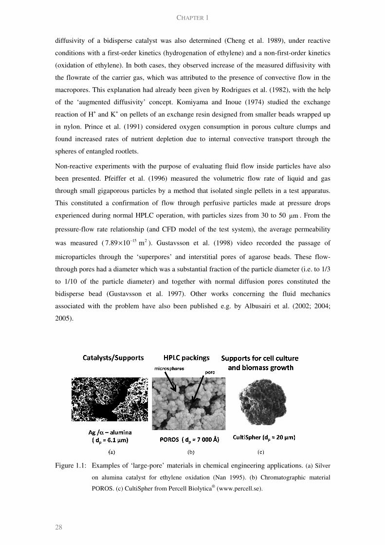
CHAPTER 1
28
diffusivity of a bidisperse catalyst was also determined (Cheng et al. 1989), under reactive
conditions with a first-order kinetics (hydrogenation of ethylene) and a non-first-order kinetics
(oxidation of ethylene). In both cases, they observed increase of the measured diffusivity with
the flowrate of the carrier gas, which was attributed to the presence of convective flow in the
macropores. This explanation had already been given by Rodrigues et al. (1982), with the help
of the ‘augmented diffusivity’ concept. Komiyama and Inoue (1974) studied the exchange
reaction of H+ and K+ on pellets of an exchange resin designed from smaller beads wrapped up
in nylon. Prince et al. (1991) considered oxygen consumption in porous culture clumps and
found increased rates of nutrient depletion due to internal convective transport through the
spheres of entangled rootlets.
Non-reactive experiments with the purpose of evaluating fluid flow inside particles have also
been presented. Pfeiffer et al. (1996) measured the volumetric flow rate of liquid and gas
through small gigaporous particles by a method that isolated single pellets in a test apparatus.
This constituted a confirmation of flow through perfusive particles made at pressure drops
experienced during normal HPLC operation, with particles sizes from 30 to 50 µm . From the
pressure-flow rate relationship (and CFD model of the test system), the average permeability
was measured ( 15 27.89 10 m−× ). Gustavsson et al. (1998) video recorded the passage of
microparticles through the ‘superpores’ and interstitial pores of agarose beads. These flow-
through pores had a diameter which was a substantial fraction of the particle diameter (i.e. to 1/3
to 1/10 of the particle diameter) and together with normal diffusion pores constituted the
bidisperse bead (Gustavsson et al. 1997). Other works concerning the fluid mechanics
associated with the problem have also been published e.g. by Albusairi et al. (2002; 2004;
2005).
Figure 1.1: Examples of ‘large-pore’ materials in chemical engineering applications. (a) Silver
on alumina catalyst for ethylene oxidation (Nan 1995). (b) Chromatographic material
POROS. (c) CultiSpher from Percell Biolytica® (www.percell.se).
OVERVIEW AND RELEVANCE
29
Other permeable materials containing large pores (say, with pore diameters greater than 500 Ǻ)
have found application for example as, (Figure 1.1):
• catalyst / supports in several reactions (Rodrigues et al. 1982; Quinta Ferreira 1988; Quinta
Ferreira et al. 1992; Nan 1995; Costa 2004; Oliveira et al. 2009; Oliveira et al. 2010;
Oliveira et al. 2011): ethylene oxidation with silver catalyst supported on α-alumina, butene
oxidation to maleic anhydride in V2O5, oxidation of o-xylene to phthalic anhydride
catalysed by V2O5, methane steam reforming…;
• HPLC packings (Afeyan et al. 1990; Lloyd et al. 1990; Carta et al. 1992; Rodrigues et al.
1995; Rodrigues 1996; Rodrigues et al. 1996; Rodrigues 1997; Leitão et al. 2002):
polystyrene materials for proteins separation like POROS (from PerSeptive Biosystems,
USA) with mean pore diameter of 7 000 Ǻ or PL4000 (from Polymer Laboratories, UK)
with pore diameter of 4 000 Ǻ;
• supports for cell culture and biomass growth (Young et al. 1987; Breitenbucher et al. 1990),
for example Cultisphere particles are used for Chinese hamster ovary cells culture from
Percell Biolytica®; and
• membrane reactors (Coelhoso et al. 1992; Golman et al. 1997; Kobayashi et al. 2001;
Kobayashi et al. 2003; Fritsch et al. 2004; Schmidt et al. 2005; Westermann et al. 2009;
Nagy 2010a; Nagy 2010b).
1.4.2 Modelling of intraparticular convection coupled with reaction in catalyst particles
The modelling studies in reaction engineering are focused mainly at the particle level. The work
from Nir and Pismen (1977) presents the first comprehensive analysis of the impact of
intraparticular convection on the performance of catalyst pellets (evaluated by the effectiveness
factor). The following remarks were made:
• a dimensionless parameter characterizes the role of convective transport and is defined as
eu L Dλ = , where L is the characteristic dimension of the pellet with diffusivity
eD and
u is the intraparticular flow velocity (usually assumed uniform);
• an order-of-magnitude analysis predicted that ~ 10λ (appreciable convective effects) when
the diameters of powder particles comprising a pellet were around 100 µm (if ~ 100Re )
and 10 µm (if 3~ 10Re ) in liquid phase, which are close to the ones used in practice;
• results for ~ 10 50λ − are presented and the higher values are possible in the case of
coarse-grained particles exposed to rapid external flow;

CHAPTER 1
30
• the effect of intraparticular convection is to increase the content of the particle in reactant,
and always results in an increase of the effectiveness factor (the minimum effectiveness is
obtained for all conditions when 0λ = );
• the effect of intraparticular flow is not visible in the limits of very slow and fast reaction
rates, where the common asymptotes for non-permeable catalyst are observed;
• the maximum enhancement of the effectiveness factor is observed in the region where
kinetics just becomes diffusion controlled (intermediate regime);
• the effectiveness factor enhancement is less pronounced in the case of sphere and cylinder
geometries, when compared to a slab.
The material balance also includes the Thiele modulus 2φ , which compares the magnitudes of
reaction and diffusion. Therefore, three regimes can be defined (as in the case of conventional
catalyst particles): chemical regime (fast diffusion compared with reaction, where presence of
the reactant in the whole slab is assured with concentration near the surface concentration);
diffusional regime (where fast reaction leads to a sharp decline in reactant concentration near
the surfaces of the slab and only a relatively small fraction of the catalyst is used) and an
intermediate regime (where the effect of moderate convection is expected to be more
noticeable), Figure 1.2.
Figure 1.2: Typical concentration profiles in the chemical, intermediate and diffusional
regimes for the problem of convection, diffusion and isothermal first-order reaction
in a slab shaped particle.
0
0.1
0.2
0.3
0.4
0.5
0.6
0.7
0.8
0.9
1
-1 -0.8 -0.6 -0.4 -0.2 0 0.2 0.4 0.6 0.8 1
2 5φ =
2 0.5φ =
2 100φ =
x
surf
c
c
10λ =fluid flow direction (uniform velocity),
chemical regime
intermediate regime
diffusional regime

OVERVIEW AND RELEVANCE
31
Table 1.5: Modelling studies involving catalytic particles with intraparticular convection
Reference Details Geometry
Komiyama et al. (1974) First-order isothermal reaction Cylinder parallel to flow
Nir and Pismen (1977) First-order isothermal reaction Slab, Sphere and Cylinder
perpendicular to flow
Nir (1977) Sequential first-order isothermal Slab and Sphere
Rodrigues et al. (1984) Zero-order isothermal reaction Slab
Cresswell (1985) Consecutive-parallel scheme
of first-order isothermal reactions
Slab
Quinta Ferreira et al. (1988;
Rodrigues et al. 1988)
First-order nonisothermal reaction Slab
* numerical solutions including steady state multiplicity
Stephanopoulos et al. (1989) Zero-order isothermal reaction Sphere
Chaara et al. (1989) Reversible first-order bimolecular reaction Slab
Lu et al. (1993) First-order isothermal reaction Slab/Sphere analogy
* transient behaviour and results for augmented diffusivity
Nan et al. (1995) First-order isothermal reaction Slab
* combined internal pressure gradients (mole changes from reaction)
Nan et al. (1996a) First-order isothermal reaction Cylinder (parallel to flow)/
Slab analogy
Nan et al. (1996b) First-order isothermal reaction Hollow Cylinder (parallel
to flow; axial convection)
* results for the augmented diffusivity by convection
Moreira et al. (1996) Isothermal Michaelis-Menten kinetics Slab
Leitão et al. (1994) Isothermal first-order reaction
* bidisperse catalysts
Slab and Sphere
Lopes et al. (1995) First-order non-isothermal reaction Sphere
* numerical solution including internal flow field
Costa (2004) First-order non-isothermal reaction
Consecutive-parallel complex scheme
Slab
* numerical solution and multiplicity analysis for external resistance to
heat transfer with internally isothermal particle
Cardoso et al. (2007) First-order nonisothermal reaction
*perturbation solutions
Slab
Nagy (2010b) First-order isothermal reaction
with external mass transfer
Slab
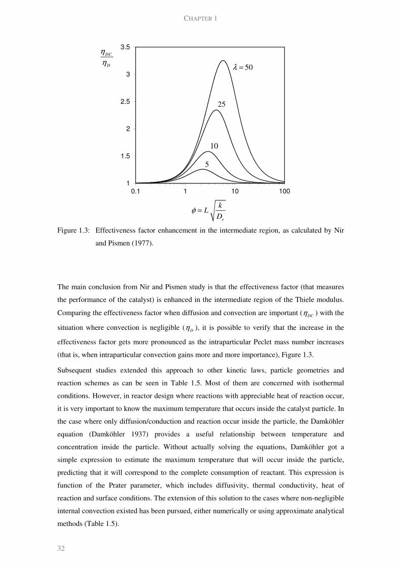
CHAPTER 1
32
Figure 1.3: Effectiveness factor enhancement in the intermediate region, as calculated by Nir
and Pismen (1977).
The main conclusion from Nir and Pismen study is that the effectiveness factor (that measures
the performance of the catalyst) is enhanced in the intermediate region of the Thiele modulus.
Comparing the effectiveness factor when diffusion and convection are important (DC
η ) with the
situation where convection is negligible (D
η ), it is possible to verify that the increase in the
effectiveness factor gets more pronounced as the intraparticular Peclet mass number increases
(that is, when intraparticular convection gains more and more importance), Figure 1.3.
Subsequent studies extended this approach to other kinetic laws, particle geometries and
reaction schemes as can be seen in Table 1.5. Most of them are concerned with isothermal
conditions. However, in reactor design where reactions with appreciable heat of reaction occur,
it is very important to know the maximum temperature that occurs inside the catalyst particle. In
the case where only diffusion/conduction and reaction occur inside the particle, the Damköhler
equation (Damköhler 1937) provides a useful relationship between temperature and
concentration inside the particle. Without actually solving the equations, Damköhler got a
simple expression to estimate the maximum temperature that will occur inside the particle,
predicting that it will correspond to the complete consumption of reactant. This expression is
function of the Prater parameter, which includes diffusivity, thermal conductivity, heat of
reaction and surface conditions. The extension of this solution to the cases where non-negligible
internal convection existed has been pursued, either numerically or using approximate analytical
methods (Table 1.5).
1
1.5
2
2.5
3
3.5
0.1 1 10 100
DC
D
η
η
e
kL
Dφ =
50λ =
25
10
5
OVERVIEW AND RELEVANCE
33
At the fixed bed reactor level, numerical solution of both steady-state and transient models with
different levels of complexity (pseudo-homogeneous and heterogeneous), including thermal
effects and runaway behaviour, were also presented (Quinta Ferreira 1988; Rodrigues et al.
1990; Ferreira et al. 1992; Costa et al. 1994; Leitao et al. 1995; Leitão et al. 1995; Quinta-
Ferreira et al. 1995; Leitão et al. 1996; Quinta Ferreira et al. 1996a; Quinta Ferreira et al. 1996b;
Leitão et al. 1998; Costa 2004).
1.5 THESIS OBJECTIVES AND OUTLINE
The main contribution of this work is to provide a comprehensive description of the transport-
reaction processes occurring in a wall-coated microchannel. We focus particularly on an
approximate analytical analysis at the individual channel level. As we have described in this
chapter, a microchannel with small aspect (diameter-to-length) ratio is an essential building
block of all microchemical systems. This geometry allows achievement of high surface-to-
volume ratios according to Eq.(1.1), and is convenient due to: easy machining, low pressure
drop, natural distribution of flow in parallel processing, and controlled residence time. Other
microgeometries such as cavities and wells have been explored for mixing purposes, but are
limited to analytical and biotechnological applications. For these reasons, the microchannel will
be our object of study. Nevertheless, the adequacy of the ‘single channel representation’ can
obviously be questioned, and it is expected to be limited when modeling arrangements which
present strong interchannel interaction due to e.g. nonuniform fluid distribution (Commenge et
al. 2002), heat exchange/losses (Di Benedetto et al. 2011) or mass transfer through porous walls
(Chen et al. 2008b) exist between channels. These cases are recognizably more expensive from
a computational point of view. However, in many situations the channel model is made general
enough to at least be included in reactor-level simulations and improve the simulation
performance of these systems. Moreover, we have already seen some cases where single
channel microreactors may work as mini-plants for production, and this may even be desirable
when high control effort and safety requirements are present. In particular, the isothermal
microchannel reactor appears as part or on its own in a number of microprocessing studies and
applications.
Due to the potential of these units, an improved understanding of their behavior is required and
this can be achieved by several modeling methods (Hardt 2000). Numerical solution of the
governing equations is able to deal with very complex systems, while exact analytical solutions
are limited to idealized models. Our perspective fits in the intermediate region between the two
approaches. On one hand, numerically obtained simulations are irremediably tied up with
particular values of the (possibly many) parameters and are associated with a certain
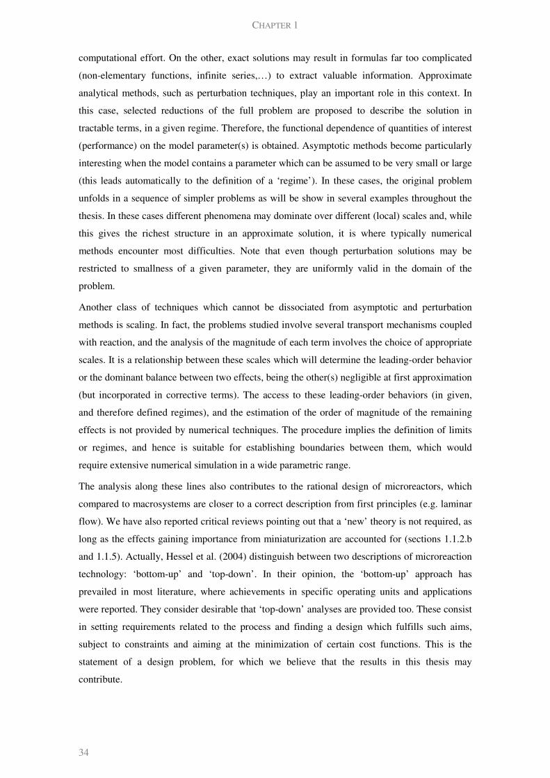
CHAPTER 1
34
computational effort. On the other, exact solutions may result in formulas far too complicated
(non-elementary functions, infinite series,…) to extract valuable information. Approximate
analytical methods, such as perturbation techniques, play an important role in this context. In
this case, selected reductions of the full problem are proposed to describe the solution in
tractable terms, in a given regime. Therefore, the functional dependence of quantities of interest
(performance) on the model parameter(s) is obtained. Asymptotic methods become particularly
interesting when the model contains a parameter which can be assumed to be very small or large
(this leads automatically to the definition of a ‘regime’). In these cases, the original problem
unfolds in a sequence of simpler problems as will be show in several examples throughout the
thesis. In these cases different phenomena may dominate over different (local) scales and, while
this gives the richest structure in an approximate solution, it is where typically numerical
methods encounter most difficulties. Note that even though perturbation solutions may be
restricted to smallness of a given parameter, they are uniformly valid in the domain of the
problem.
Another class of techniques which cannot be dissociated from asymptotic and perturbation
methods is scaling. In fact, the problems studied involve several transport mechanisms coupled
with reaction, and the analysis of the magnitude of each term involves the choice of appropriate
scales. It is a relationship between these scales which will determine the leading-order behavior
or the dominant balance between two effects, being the other(s) negligible at first approximation
(but incorporated in corrective terms). The access to these leading-order behaviors (in given,
and therefore defined regimes), and the estimation of the order of magnitude of the remaining
effects is not provided by numerical techniques. The procedure implies the definition of limits
or regimes, and hence is suitable for establishing boundaries between them, which would
require extensive numerical simulation in a wide parametric range.
The analysis along these lines also contributes to the rational design of microreactors, which
compared to macrosystems are closer to a correct description from first principles (e.g. laminar
flow). We have also reported critical reviews pointing out that a ‘new’ theory is not required, as
long as the effects gaining importance from miniaturization are accounted for (sections 1.1.2.b
and 1.1.5). Actually, Hessel et al. (2004) distinguish between two descriptions of microreaction
technology: ‘bottom-up’ and ‘top-down’. In their opinion, the ‘bottom-up’ approach has
prevailed in most literature, where achievements in specific operating units and applications
were reported. They consider desirable that ‘top-down’ analyses are provided too. These consist
in setting requirements related to the process and finding a design which fulfills such aims,
subject to constraints and aiming at the minimization of certain cost functions. This is the
statement of a design problem, for which we believe that the results in this thesis may
contribute.
OVERVIEW AND RELEVANCE
35
We aim to achieve further insight into the considered transport-reaction problem with the
following two main objectives:
i. provide accurate approximate results from reduced-order models without the need for
numerically calculated quantities, and
ii. identify the limits to which the full problem reduces, mapping operating regimes and the
transitions between them.
These goals will allow us to analyze relevant process intensification strategies, such as
microreactors and flow-through permeable catalyst particles. The relevance of both was
highlighted in this chapter, and in practice they are considered as promising directions,
particularly for fast reactions with highly active catalysts. For example, information from
Velocys, Inc. concerning the choice of reactor design for reactions such as oxidations is
presented in Figure 1.4 in terms of the kinetic rate and the amount of pressure drop or
temperature variation allowed.
Figure 1.4: Velocys, Inc. catalyst selection strategy. Adapted from J. Lerou, ‘Microreaction
Engineering: Is small really better?’ (www.velocys.com).

CHAPTER 1
36
In particular, this work proposes:
1. a solution for the transport-reaction problem inside a wall-coated microchannel for finite
reaction rates in the fully developed and developing limits of the concentration profile
(Chapter 2);
2. a description of conversion in a microchannel when reactions with nonlinear kinetics occur
in the asymptotic limits of small and large reaction rates (Chapter 2);
3. a uniform solution which combines classic theories of mass and heat transfer in channel
flow and defines ranges of validity for the limits (Chapter 3); and
4. a regime map where a comprehensive picture of the different interphase transport – reaction
behaviors is plotted, and boundaries between them derived (Chapter 4).
We also consider the problem at the level of a thin catalytic coating, to achieve:
5. the calculation of the approximate effectiveness factor with linear and nonlinear kinetics
and nonuniform geometries (Chapter 5); and
6. the definition of regimes considering the interplay between internal and external mass
transfer (Chapter 5).
Furthermore, the existence of intraparticular convection effects is studied in two contexts:
7. calculation of a ‘curvature correction’ for isothermal linear kinetics in a channel with a thin
perfusive wall, and identification of the conditions for maximum enhancement (Chapter 5),
and
8. study of the influence of nonisothermal effects in a permeable slab with focus on
effectiveness factor and maximum temperature estimation (Chapter 6).
Finally, the main conclusions of our analysis and suggestions for future work are presented in
Chapter 7.
NOTATION
a channel’s characteristic (transverse) dimension
chA cross-sectional area of the channel
0c reference concentration
PC fluid specific heat
D fluid’s bulk diffusivity
chd channel’s hydraulic diameter

OVERVIEW AND RELEVANCE
37
partd particle diameter
GHSV gas hourly space velocity
kh coefficient in Carman-Kozeney equation (double of the ratio between length of passage
in porous bed and in straight capillary)
k reaction rate kinetic constant (referred to catalyst volume)
heatk heat transfer coefficient
mk mass transfer coefficient
surfk reaction rate kinetic constant (referred to catalyst surface area)
RH∆ heat of reaction
meanℓ mean free path
L channel’s length, axial characteristic dimension
m order of reaction with power-law kinetics
mɺ mass flowrate
chN number of channels
Nu Nusselt number
NTU Number of transfer units
P∆ Pressure drop
Pr Prandtl’s number
feedQ feed flowrate
( )cR reaction rate (referred to catalyst volume)
Re Reynold’s number
surfS channel surface area
Sc Schmidt’s number
Sh Sherwood number
wt catalytic coating thickness
0T reference temperature
adT∆ adiabatic temperature rise
u average fluid velocity in the channel
V channel’s volume
Greek letters
ε porosity
δ boundary layer thickness
κ fluid thermal diffusivity, ( )PCλ ρ
λ fluid thermal conductivity
η effectiveness factor
ρ fluid’s density
ν fluid’s kinematic viscosity
τ timescale, characteristic time, time constant

CHAPTER 1
38
Subscripts
bulk conditions in the channel’s bulk
surf conditions at the channel/catalyst interface
wall referred to wall material
REFERENCES
Afeyan, N. B., S. P. Fulton, N. F. Gordon, I. Mazsaroff, L. Varady and F. E. Regnier (1990). "Perfusion chromatography: An approach to purifying biomolecules." Nature Biotechnology 8(3): 203-206.
Albusairi, B. and J. T. Hsu (2002). "Application of shape factor to determine the permeability of perfusive particles." Chemical Engineering Journal 89(1-3): 173-183.
Albusairi, B. and J. T. Hsu (2004). "Flow through beds of perfusive particles: Effective medium model for velocity prediction within the perfusive media." Chemical Engineering Journal 100(1-3): 79-84.
Albusairi, B. H. and J. T. Hsu (2005). "Dispersion coefficient prediction within a bed packed with perfusive particles." AIChE Journal 51(5): 1330-1338.
Aris, R. (1956). "On the Dispersion of a Solute in a Fluid Flowing through a Tube " Proceedings of the Royal Society of London A 235(1200): 67-77.
Becht, S., R. Franke, A. Geißelmann and H. Hahn (2009). "An industrial view of process intensification." Chemical Engineering and Processing: Process Intensification 48(1): 329-332.
Becht, S., R. Franke, A. Gießelmann and H. Hahn (2007). "Micro process technology as a means of process intensification." Chemical Engineering and Technology 30(3): 295-299.
Benito-López, F., R. J. M. Egberink, D. N. Reinhoudt and W. Verboom (2008). "High pressure in organic chemistry on the way to miniaturization." Tetrahedron 64(43): 10023-10040.
Beretta, A., G. Groppi, L. Majocchi and P. Forzatti (1999). "Potentialities and draw-backs of the experimental approach to the study of high T and high GHSV kinetics." Applied Catalysis A: General 187(1): 49-60.
Bird, R. B., W. E. Stewart and E. N. Lightfoot (2002). Transport Phenomena. New York, John Wiley & Sons, Inc.
Bolivar, J. M., J. Wiesbauer and B. Nidetzky (2011). "Biotransformations in microstructured reactors: more than flowing with the stream?" Trends in Biotechnology.
Breitenbucher, K., M. Siegl, A. Knupfer and M. Radke (1990). "Open-pore sintered glass as a high-efficiency support medium in bioreactors: New results and long-term experiences achieved in high-rate anaerobic digestion." Water Science and Technology 22(1-2): 25-32.
Bruus, H. (2008). Theoretical Microfluidics. New York, Oxford University Press.
Cardoso, S. S. S. and A. E. Rodrigues (2007). "Convection, diffusion and reaction in a nonisothermal, porous catalyst slab." AIChE Journal 53(5): 1325-1336.
OVERVIEW AND RELEVANCE
39
Carta, G., M. E. Gregory, D. J. Kirwan and H. A. Massaldi (1992). "Chromatography with permeable supports: Theory and comparison with experiments." Separations Technology 2(2): 62-72.
Casanovas, A., C. de Leitenburg, A. Trovarelli and J. Llorca (2008a). "Catalytic monoliths for ethanol steam reforming." Catalysis Today 138(3-4): 187-192.
Casanovas, A., M. Dominguez, C. Ledesma, E. Lopez and J. Llorca (2008b). "Catalytic walls and micro-devices for generating hydrogen by low temperature steam reforming of ethanol." Catalysis Today 143(1-2): 32-37
Chaara, M. and R. Noble (1989). "Effect of Convective Flow Across a Film on Facilitated Transport." Separation Science and Technology 24: 893-903.
Charpentier, J. C. (2005). "Process intensification by miniaturization." Chemical Engineering and Technology 28(3): 255-258.
Chen, H., H. Yu, Y. Tang, M. Pan, F. Peng, H. Wang and J. Yang (2008a). "Assessment and optimization of the mass-transfer limitation in a metal foam methanol microreformer." Applied Catalysis A: General 337(2): 155-162.
Chen, J., H. Yang, N. Wang, Z. Ring and T. Dabros (2008b). "Mathematical modeling of monolith catalysts and reactors for gas phase reactions." Applied Catalysis A: General 345(1): 1-11.
Cheng, S. and A. Zoulalian (1989). "Influence de la reaction chimique et de la convection interne sur la determination de la diffusivite apparente d'un catalyseur." Chemical Engineering Journal 41(2): 91-104.
Cheng, S., A. Zoulalian and J. P. Brunelle (1987). Influence of the porous structure of alumina pellets and the internal convective flow on the effective diffusivity of exhaust gas catalyst. Catalysis and Automative Pollution Control. A. Crucq and A. Frennet. Amsterdam, Elsevier Science Publishers B.V.: 323-332.
Coelhoso, I., J. Crespo and A. E. Rodrigues (1992). The effect of convective flow on the facilitated transport across a membrane. Meeting of the European Membrane Society. Paris.
Cogan, R., G. Pipko and A. Nir (1982). "Simultaneous Intraparticle Forced Convection, Diffusion and Reaction in a Porous Catalyst - 3." Chemical Engineering Science 37(2): 147-151.
Commenge, J. M., L. Falk, J. P. Corriou and M. Matlosz (2002). "Optimal Design for Flow Uniformity in Microchannel Reactors." AIChE Journal 48(2): 345-358.
Commenge, J. M., L. Falk, J. P. Corriou and M. Matlosz (2005). "Analysis of microstructured reactor characteristics for process miniaturization and intensification." Chemical Engineering and Technology 28(4): 446-458.
Costa, A. C. (2004). Estudo do comportamento estacionário e dinâmico de reactores catalíticos de leito fixo com convecção intraparticular. Universidade de Coimbra. PhD thesis.
Costa, C. A., R. M. Quinta Ferreira and A. E. Rodrigues (1994). "Wrong-way behavior in packed-bed reactors with 'large-pore' catalysts." Chemical Engineering Science 49(24 B): 5571-5583.
Cresswell, D. L. (1985). "Intra-particle convection: its measurement and effect on catalyst activity and selectivity." Applied catalysis 15(1): 103-116.
Cybulski, A. and J. Moulijn (1998). Structured Catalysts and Reactors. New York, Marcel Dekker.
Damköhler, G. (1937). "Einfluss von Diffusion, Strömung, und Wärmetransport auf die Ausbeute in Chemisch-Technischen Reaktionen." Chem.-Eng.-Tech 3(Part 1, Chapter 2): 359-485.

CHAPTER 1
40
Delsman, E. R., A. Pierik, M. H. J. M. De Croon, G. J. Kramer and J. C. Schouten (2004). "Microchannel plate geometry optimization for even flow distribution at high flow rates." Chemical Engineering Research and Design 82(2): 267-273.
Deshmukh, S. R., A. L. Y. Tonkovich, K. T. Jarosch, L. Schrader, S. P. Fitzgerald, D. R. Kilanowski, J. J. Lerou and T. J. Mazanec (2010). "Scale-up of microchannel reactors for Fischer-Tropsch synthesis." Industrial and Engineering Chemistry Research 49(21): 10883-10888.
Di Benedetto, A. and V. Di Sarli (2011). "CFD Modeling and Simulation of a Catalytic Micro-Monolith." International Journal of Chemical Reactor Engineering 9.
Ebrahimi, F., E. Kolehmainen, P. Oinas, V. Hietapelto and I. Turunen (2011). "Production of unstable percarboxylic acids in a microstructured reactor." Chemical Engineering Journal 167(2-3): 713-717.
Ebrahimi, F., E. Kolehmainen and I. Turunen (2009). "Safety advantages of on-site microprocesses." Organic Process Research and Development 13(5): 965-969.
Ehrfeld, W., V. Hessel and H. Löwe (2000). Microreactors: New technology for modern chemistry. Weinheim, Wiley-VCH.
Falk, L. and J. M. Commenge (2010). "Performance comparison of micromixers." Chemical Engineering Science 65(1): 405-411.
Federici, J. A. and D. G. Vlachos (2011). "Experimental studies on syngas catalytic combustion on Pt/Al2O3 in a microreactor." Combustion and Flame In Press.
Ferreira, R. M. Q., A. C. Costa and A. E. Rodrigues (1992). "Dynamic behavior of fixed-bed reactors with ``large-pore'' catalysts: A bidimensional heterogeneous diffusion/convection model." Computers and Chemical Engineering 16(8): 721-751.
Fritsch, D., I. Randjelovic and F. Keil (2004). "Application of a forced-flow catalytic membrane reactor for the dimerisation of isobutene." Catalysis Today 98(1-2 SPEC. ISS.): 295-308.
Germani, G. and Y. Schuurman (2006). "Water-gas shift reaction kinetics over micro-structured Pt/CeO2/AI2O3 catalysts." AIChE Journal 52(5): 1806-1813.
Gokhale, S. V., V. K. Jayaraman, R. K. Tayal and B. D. Kulkarni (2005). "Microchannel reactors: Applications and use in process development." International Journal of Chemical Reactor Engineering 3.
Golman, B., K. Shinohara and M. Kobayashi (1997). "Selectivity and yield of exothermic consecutive reactions in catalytically active porous membrane reactor." Journal of Chemical Engineering of Japan 30(3): 507-513.
Görke, O., P. Pfeifer and K. Schubert (2009). "Kinetic study of ethanol reforming in a microreactor." Applied Catalysis A: General 360(2): 232-241.
Groppi, G., W. Ibashi, M. Valentini and P. Forzatti (2001). "High-temperature combustion of CH4 over PdO/Al2O3: Kinetic measurements in a structured annular reactor." Chemical Engineering Science 56(3): 831-839.
Gustavsson, P. E., A. Axelsson and P. O. Larsson (1998). "Direct measurements of convective fluid velocities in superporous agarose beads." Journal of Chromatography A 795(2): 199-210.
Gustavsson, P. E., K. Mosbach, K. Nilsson and P. O. Larsson (1997). "Superporous agarose as an affinity chromatography support." Journal of Chromatography A 776(2): 197-203.

OVERVIEW AND RELEVANCE
41
Halder, R., A. Lawal and R. Damavarapu (2007). "Nitration of toluene in a microreactor." Catalysis Today 125(1-2): 74-80.
Hardt, S. (2000). Microreactors – Modeling and Simulation. Ullmann's Encyclopedia of Industrial Chemistry, Wiley-VCH Verlag GmbH & Co. KGaA.
Hardt, S., W. Ehrfeld, V. Hessel and K. M. Vanden Bussche (2003). "Strategies for size reduction of microreactors by heat transfer enhancement effects." Chemical Engineering Communications 190(4): 540-559.
Hawtin, P. and R. Murdoch (1964). "The Role of In-pore Mass Transport Resistance in the Reaction of Porous Solids with Gases." Chemical Engineering Science 19: 819-834.
Hayes, R. E. and S. T. Kolaczkowski (1994). "Mass and heat transfer effects in catalytic monolith reactors." Chemical Engineering Science 49(21): 3587-3599.
Hayes, R. E., S. T. Kolaczkowski, W. J. Thomas and J. Titiloye (1995). "Intraphase diffusion and interphase mass transfer effects during the catalytic oxidation of CO in a tube wall reactor." Proceedings - Royal Society of London, A 448(1933): 321-334.
Herwig, H. (2008). Momentum and Heat Transfer in Microsized Devices. Micro Process Engineering: Fundamentals, Devices, Fabrication, and Applications. N. Kockmann. Weinheim, Germany, Wiley-VCH Verlag GmbH: 47-70.
Hessel, V. (2009). "Process windows - gate to maximizing process intensification via flow chemistry." Chemical Engineering and Technology 32(11): 1655-1681.
Hessel, V., B. Cortese and M. H. J. M. de Croon (2011). "Novel process windows - Concept, proposition and evaluation methodology, and intensified superheated processing." Chemical Engineering Science 66(7): 1426-1448.
Hessel, V., S. Hardt and H. Löwe (2004). Chemical Micro Process Engineering: Fundamentals, Modelling and Reactions. Weinheim, Wiley-VCH.
Hessel, V., C. Hofmann, P. Löb, J. Löhndorf, H. Löwe and A. Ziogas (2005a). "Aqueous Kolbe-Schmitt synthesis using resorcinol in a microreactor laboratory rig under high-p,T conditions." Organic Process Research and Development 9(4): 479-489.
Hessel, V., C. Knobloch and H. Löwe (2008a). "Review on Patents in Microreactor and Micro Process Engineering." Recent Patents on Chemical Engineering 1(1): 1-16.
Hessel, V., D. Kralisch and U. Krtschil (2008b). "Sustainability through green processing - Novel process windows intensify micro and milli process technologies." Energy and Environmental Science 1(4): 467-478.
Hessel, V., H. Löwe, A. Müller and G. Kolb (2005b). Chemical Micro Process Engineering: Processing and Plants. Weinheim, Wiley-VCH.
Hoebink, J. H. B. J. and G. B. Marin (1998). Modeling of Monolithic Reactors for Automotive Exhaust Gas Treatment. Structured Catalysts and Reactors. A. Cybulski and J. Moulijn. New York, Marcel Dekker: 209-237.
Illg, T., V. Hessel, P. Löb and J. C. Schouten (2011). "Novel Process Window for the safe and continuous synthesis of tert.-butyl peroxy pivalate in a micro-reactor." Chemical Engineering Journal 167(2-3): 504-509.

CHAPTER 1
42
Illg, T., P. Löb and V. Hessel (2010). "Flow chemistry using milli- and microstructured reactors-From conventional to novel process windows." Bioorganic and Medicinal Chemistry 18(11): 3707-3719.
Jensen, K. F. (2001). "Microreaction engineering-is small better?" Chemical Engineering Science 56(2): 293-303.
Judy, J., D. Maynes and B. W. Webb (2002). "Characterization of frictional pressure drop for liquid flows through microchannels." International Journal of Heat and Mass Transfer 45(17): 3477-3489.
Kapteijn, F., R. M. De Deugd and J. A. Moulijn (2005). "Fischer-Tropsch synthesis using monolithic catalysts." Catalysis Today 105(3-4): 350-356.
Kestenbaum, H., A. L. De Oliveira, W. Schmidt, F. Schüth, W. Ehrfeld, K. Gebauer, H. Löwe, T. Richter, D. Lebiedz, I. Untiedt and H. Zücher (2002). "Silver-catalyzed oxidation of ethylene to ethylene oxide in a microreaction system." Industrial and Engineering Chemistry Research 41(4): 710-719.
Kim, K. Y., J. Han, S. W. Nam, T. H. Lim and H. I. Lee (2008). "Preferential oxidation of CO over CuO/CeO2 and Pt-Co/Al2O3 catalysts in micro-channel reactors." Catalysis Today 131(1-4): 431-436.
Kobayashi, M., T. Kanno, J. I. Horiuchi, S. Hoshi, N. Hattori and J. Togawa (2001). Hysteresis kinetics of propene oxidation characterized by a Ag-Re supported membrane reactor. 133: 105-112.
Kobayashi, M., J. Togawa, T. Kanno, J. I. Horiuchi and K. Tada (2003). "Dramatic innovation of propene epoxidation efficiency derived from a forced flow membrane reactor." Journal of Chemical Technology and Biotechnology 78(2-3): 303-307.
Kockmann, N. and D. M. Roberge (2009). "Harsh reaction conditions in continuous-flow microreactors for pharmaceutical production." Chemical Engineering and Technology 32(11): 1682-1694.
Kolaczkowski, S. T. (1999). "Modelling catalytic combustion in monolith reactors - Challenges faced." Catalysis Today 47(1-4): 209-218.
Kolb, G., V. Cominos, C. Hofmann, H. Pennemann, J. Schürer, D. Tiemann, M. Wichert, R. Zapf, V. Hessel and H. Löwe (2005). "Integrated microstructured fuel processors for fuel cell applications." Chemical Engineering Research and Design 83(6 A): 626-633.
Kolb, G. and V. Hessel (2004). "Micro-structured reactors for gas phase reactions." Chemical Engineering Journal 98(1-2): 1-38.
Kolb, G., V. Hessel, V. Cominos, C. Hofmann, H. Löwe, G. Nikolaidis, R. Zapf, A. Ziogas, E. R. Delsman, M. H. J. M. de Croon, J. C. Schouten, O. de la Iglesia, R. Mallada and J. Santamaria (2007). "Selective oxidations in micro-structured catalytic reactors-For gas-phase reactions and specifically for fuel processing for fuel cells." Catalysis Today 120(1): 2-20.
Komiyama, H. and H. Inoue (1974). "Effects of intraparticle flow on catalytic reactions." Journal of Chemical Engineering of Japan 7(4): 281-286.
Kreutzer, M. T., F. Kapteijn and J. A. Moulijn (2006). "Shouldn't catalysts shape up? Structured reactors in general and gas-liquid monolith reactors in particular." Catalysis Today 111(1-2): 111-118.
Kreutzer, M. T., F. Kapteijn, J. A. Moulijn and J. J. Heiszwolf (2005). "Multiphase monolith reactors: Chemical reaction engineering of segmented flow in microchannels." Chemical Engineering Science 60(22): 5895-5916.
Kundu, A., J. E. Ahn, S. S. Park, Y. G. Shul and H. S. Han (2008). "Process intensification by micro-channel reactor for steam reforming of methanol." Chemical Engineering Journal 135(1-2): 113-119.
OVERVIEW AND RELEVANCE
43
Lee, P. S., S. V. Garimella and D. Liu (2005). "Investigation of heat transfer in rectangular microchannels." International Journal of Heat and Mass Transfer 48(9): 1688-1704.
Leitao, A., M. Dias and A. Rodrigues (1994). "Effectiveness of bidisperse catalysts with convective flow in the macropores." Chemical Engineering Journal and the Biochemical Engineering Journal 55(1-2): 81-86.
Leitão, A., M. Li and A. Rodrigues (2002). "The role of intraparticle convection in protein adsorption by liquid chromatography using POROS 20 HQ/M particles." Biochemical Engineering Journal 11(1): 33-48.
Leitao, A. and A. Rodrigues (1995). "Influence of intraparticle convection on product distribution for series-parallel catalytic reactions." Chemical Engineering Research and Design 73(A2): 130-135.
Leitão, A. and A. Rodrigues (1995). "Catalytic processes using "large-pore" materials: effects of the flow rate and operating temperature on the conversion in a plug-flow reactor for irreversible first-order reactions." The Chemical Engineering Journal and The Biochemical Engineering Journal 60(1-3): 111-116.
Leitão, A. and A. Rodrigues (1996). "Modeling of biodegradation/adsorption combined processes in fixed-bed biofilm reactors: Effects of the intraparticle convective flow." Chemical Engineering Science 51(20): 4595-4604.
Leitão, A. and A. Rodrigues (1998). "Dynamic behaviour of a fixed-bed biofilm reactor: Analysis of the role of the intraparticle convective flow under biofilm growth." Biochemical Engineering Journal 2(1): 1-9.
Lerou, J. J., A. L. Tonkovich, L. Silva, S. Perry and J. McDaniel (2010). "Microchannel reactor architecture enables greener processes." Chemical Engineering Science 65(1): 380-385.
Lin, C. C. and L. A. Segel (1988). Mathematics Applied to Deterministic Problems in the Natural Sciences, SIAM.
Lloyd, L. L. and F. P. Warner (1990). "Preparative high-performance liquid chromatography on a unique high-speed macroporous resin." Journal of Chromatography A 512(C): 365-376.
Lomel, S., L. Falk, J. M. Commenge, J. L. Houzelot and K. Ramdani (2006). "The microreactor: A systematic and efficient tool for the transition from batch to continuous process?" Chemical Engineering Research and Design 84(5 A): 363-369.
Lopes, J. C. B., M. M. Dias, V. G. Mata and A. E. Rodrigues (1995). "Flow field and non-isothermal effects on diffusion, convection, and reaction in permeable catalysts." Industrial and Engineering Chemistry Research 34(1): 148-157.
Lu, Z. P., M. M. Dias, J. C. B. Lopes, G. Carta and A. E. Rodrigues (1993). "Diffusion, convection, and reaction in catalyst particles: Analogy between slab and sphere geometries." Industrial and Engineering Chemistry Research 32(9): 1839-1852.
Lucas, M. and P. Claus (2003). "High throughput screening in monolith reactors for total oxidation reactions." Applied Catalysis A: General 254(1): 35-43.
Mae, K. (2007). "Advanced chemical processing using microspace." Chemical Engineering Science 62(18-20): 4842-4851.
Maehara, S., M. Taneda and K. Kusakabe (2008). "Catalytic synthesis of hydrogen peroxide in microreactors." Chemical Engineering Research and Design 86(4): 410-415.

CHAPTER 1
44
Marre, S., A. Adamo, S. Basak, C. Aymonier and K. F. Jensen (2010). "Design and packaging of microreactors for high pressure and high temperature applications." Industrial and Engineering Chemistry Research 49(22): 11310-11320.
McCarty, J. G. (1995). "Kinetics of PdO combustion catalysis." Catalysis Today 26(3-4): 283-293.
McMullen, J. P. and K. F. Jensen (2010). Integrated microreactors for reaction automation: New approaches to reaction development. 3: 19-42.
Mills, P. L., D. J. Quiram and J. F. Ryley (2007). "Microreactor technology and process miniaturization for catalytic reactions--A perspective on recent developments and emerging technologies." Chemical Engineering Science 62(24): 6992-7010.
Miyazaki, M. and H. Maeda (2006). "Microchannel enzyme reactors and their applications for processing." Trends in Biotechnology 24(10): 463-470.
Moreira, N. E. and F. X. Malcata (1996). "Use of convective flow to enhance the effectiveness factor of poroys slab-shaped beads with immobilized enzyme." Journal of Chemical Engineering of Japan 29(2): 392-395.
Moulijn, J., M. Kreutzer and F. Kapteijn (2005). "A little structure works wonders." Chemical Engineer(768): 32-34.
Nagy, E. (2010a). "Convective and diffusive mass transport through anisotropic, capillary membrane." Chemical Engineering and Processing: Process Intensification 49(7): 716-721.
Nagy, E. (2010b). "Mass transfer through a convection flow catalytic membrane layer with dispersed nanometer-sized catalyst." Industrial and Engineering Chemistry Research 49(3): 1057-1062.
Nan, H. S. (1995). Influence of forced convection on mass transport and reaction in porous catalysts pellets and reactor performance. University of Porto. PhD thesis.
Nan, H. S., M. M. Dias, J. C. B. Lopes and A. E. Rodrigues (1996a). "Diffusion, convection and reaction in catalyst particles: Analogy between slab and cylinder geometries." Chemical Engineering Journal and the Biochemical Engineering Journal 61(2): 113-122.
Nan, H. S., M. M. Dias, V. G. Mata and A. E. Rodrigues (1996b). "Measurements of effective diffusivity in large-pore permeable pellets with various geometries using the chromatographic method." Chemical Engineering Communications 146: 201-229.
Nan, H. S., M. M. Dias and A. E. Rodrigues (1995). "Effect of forced convection on reaction with mole changes in porous catalysts." Chemical Engineering Journal and the Biochemical Engineering Journal 57(2): 101-114.
Nieuwland, P. J., K. Koch, N. Van Harskamp, R. Wehrens, J. C. M. Van Hest and F. P. J. T. Rutjes (2010). "Flash chemistry extensively optimized: High-temperature Swern-Moffatt oxidation in an automated microreactor platform." Chemistry - An Asian Journal 5(4): 799-805.
Nijhuis, T. A., M. T. Kreutzer, A. C. J. Romijn, F. Kapteijn and J. A. Moulijn (2001). "Monolithic catalysts as more efficient three-phase reactors." Catalysis Today 66(2-4): 157-165.
Nir, A. (1977). "Simultaneous intraparticle forced convection, diffusion and reaction in a porous catalyst - 2. Selectivity of sequential reactions." Chemical Engineering Science 32(8): 925-930.
Nir, A. and L. M. Pismen (1977). "Simultaneous intraparticle forced convection, diffusion and reaction in a porous catalyst." Chemical Engineering Science 32(1): 35-41.

OVERVIEW AND RELEVANCE
45
Oh, S. H. and J. C. Cavendish (1982). "Transients of monolithic catalytic converters: Response to step changes in feedstream temperature as related to controlling automobile emissions." Industrial & Engineering Chemistry Product Research and Development 21(1): 29-37.
Oliveira, E. L. G., C. A. Grande and A. E. Rodrigues (2009). "Steam methane reforming in a Ni/Al2O3 Catalyst: Kinetics and diffusional limitations in extrudates." Canadian Journal of Chemical Engineering 87(6): 945-956.
Oliveira, E. L. G., C. A. Grande and A. E. Rodrigues (2010). "Methane steam reforming in large pore catalyst." Chemical Engineering Science 65(5): 1539-1550.
Oliveira, E. L. G., C. A. Grande and A. E. Rodrigues (2011). "Effect of catalyst activity in SMR-SERP for hydrogen production: Commercial vs. large-pore catalyst." Chemical Engineering Science 66(3): 342-354.
Pennemann, H., P. Watts, S. J. Haswell, V. Hessel and H. Löwe (2004). "Benchmarking of microreactor applications." Organic Process Research and Development 8(3): 422-439.
Pfeiffer, J. F., J. C. Chen and J. T. Hsu (1996). "Permeability of Gigaporous Particles." AIChE Journal 42(4): 932-939.
Pfund, D., D. Rector, A. Shekarriz, A. Popescu and J. Welty (2000). "Pressure drop measurements in a microchannel." AIChE Journal 46(8): 1496-1507.
Prince, C. L., V. Bringi and M. L. Shuler (1991). "Convective Mass Transfer in Large Porous Biocatalysts: Plant Organ Cultures." Biotechnology Progress 7(2): 195-199.
Quinta-Ferreira, R. M., P. M. Simoes and A. E. Rodrigues (1995). "Simulation of tubular reactors packed with large-pore catalysts with spherical geometry." Computers and Chemical Engineering 19(Suppl): S351-S356.
Quinta Ferreira, R. M. (1988). Contribuição para o Estudo de Reactores Catalíticos de leito fixo. Efeito da convecção em catalisadores de poros largos e casos de catalisadores bidispersos. University of Porto. PhD Thesis.
Quinta Ferreira, R. M., C. A. Almeida-Costa and A. E. Rodrigues (1996a). "Effect of intraparticle convection on the transient behavior of fixed-bed reactors: Finite differences and collocation methods for solving unidimensional models." Computers and Chemical Engineering 20(10): 1201-1225.
Quinta Ferreira, R. M., C. A. Almeida-Costa and A. E. Rodrigues (1996b). "Heterogeneous models of tubular reactors packed with ion-exchange resins: Simulation of the MTBE synthesis." Industrial and Engineering Chemistry Research 35(11): 3827-3841.
Quinta Ferreira, R. M., M. M. Marques, M. F. Babo and A. E. Rodrigues (1992). "Modelling of the methane steam reforming reactor with large-pore catalysts." Chemical Engineering Science 47(9-11): 2909-2914.
Razzaq, T., T. N. Glasnov and C. O. Kappe (2009). "Accessing novel process windows in a high-temperature/pressure capillary flow reactor." Chemical Engineering and Technology 32(11): 1702-1716.
Razzaq, T. and C. O. Kappe (2010). "Continuous flow organic synthesis under high-temperature/pressure conditions." Chemistry - An Asian Journal 5(6): 1274-1289.
Rebrov, E. V., A. Berenguer-Murcia, H. E. Skelton, B. F. G. Johnson, A. E. H. Wheatley and J. C. Schouten (2009). "Capillary microreactors wall-coated with mesoporous titania thin film catalyst supports." Lab on a Chip - Miniaturisation for Chemistry and Biology 9(4): 503-506.

CHAPTER 1
46
Rebrov, E. V., R. P. Ekatpure, M. H. J. M. De Croon and J. C. Schouten (2007a). "Design of a thick-walled screen for flow equalization in microstructured reactors." Journal of Micromechanics and Microengineering 17(3): 633-641.
Rebrov, E. V., I. Z. Ismagilov, R. P. Ekatpure, M. H. J. M. De Croon and J. C. Schouten (2007b). "Header design for flow equalization in microstructured reactors." AIChE Journal 53(1): 28-38.
Renken, A. and L. Kiwi-Minsker (2008). Chemical Reactions in Continuous–flow Microstructured Reactors. Micro Process Engineering: Fundamentals, Devices, Fabrication, and Applications. N. Kockmann. Weinheim, Germany, Wiley-VCH Verlag GmbH: 173-201.
Roberge, D. M., N. Bieler, M. Mathier, M. Eyholzer, B. Zimmermann, P. Barthe, C. Guermeur, O. Lobet, M. Moreno and P. Woehl (2008). "Development of an industrial multi-injection microreactor for fast and exothermic reactions - Part II." Chemical Engineering and Technology 31(8): 1155-1161.
Roberge, D. M., L. Ducry, N. Bieler, P. Cretton and B. Zimmermann (2005). "Microreactor technology: A revolution for the fine chemical and pharmaceutical industries?" Chemical Engineering and Technology 28(3): 318-323.
Rodrigues, A., B. Ahn and A. Zoulalian (1982). "Intraparticle Forced Convection Effect in Catalyst Diffusivity Measurements and Reactor Design." AIChE Journal 28: 541-546.
Rodrigues, A. E. (1996). "Intraparticle Convection in Chromatographic Permeable Packings." ACS Symposium Series 635: 157-172.
Rodrigues, A. E. (1997). "Permeable packings and perfusion chromatography in protein separation." Journal of Chromatography B: Biomedical Applications 699(1-2): 47-61.
Rodrigues, A. E., C. Chenou and M. De La Rendueles Vega (1996). "Protein separation by liquid chromatography using permeable POROS Q/M particles." Chemical Engineering Journal and the Biochemical Engineering Journal 61(3): 191-201.
Rodrigues, A. E., J. M. Loureiro, C. Chenou and M. Rendueles de la Vega (1995). "Bioseparations with permeable particles." Journal of Chromatography B: Biomedical Applications 664(1): 233-240.
Rodrigues, A. E., J. M. Orfao and A. Zoulalian (1984). "Intraparticle convection, diffusion and zero order reaction in porous catalysts." Chemical Engineering Communications 27(5-6): 327-337.
Rodrigues, A. E. and R. M. Quinta Ferreira (1988). "Convection, diffusion and reaction in a large-pore catalyst particle." AIChE Symposium Series 84(266): 80-87.
Rodrigues, A. E. and R. M. Quinta Ferreira (1990). "Effect of intraparticle convection on the steady-state behavior of fixed-bed catalytic reactors." Chemical Engineering Science 45(8): 2653-2660.
Rosa, P., T. G. Karayiannis and M. W. Collins (2009). "Single-phase heat transfer in microchannels: The importance of scaling effects." Applied Thermal Engineering 29(17-18): 3447-3468.
Sazonova, N. N., S. N. Pavlova, S. A. Pokrovskaya, N. A. Chumakova and V. A. Sadykov (2009). "Structured reactor with a monolith catalyst fragment for kinetic studies. The case of CH4 partial oxidation on LaNiPt-catalyst." Chemical Engineering Journal 154(1-3): 17-24.
Scheidtmann, J., P. A. Weiß and W. F. Maier (2001). "Hunting for better catalysts and materials-combinatorial chemistry and high throughput technology." Applied Catalysis A: General 222(1-2): 79-89.
Schmidt, A., R. Haidar and R. Schomäcker (2005). "Selectivity of partial hydrogenation reactions performed in a pore-through-flow catalytic membrane reactor." Catalysis Today 104(2-4): 305-312.

OVERVIEW AND RELEVANCE
47
Shah, R. K. and A. L. London (1978). Laminar flow forced convection in ducts. New York, Academic Press.
Srinivasan, R., I. M. Hsing, P. E. Berger, K. F. Jensen, S. L. Firebaugh, M. A. Schmidt, M. P. Harold, J. J. Lerou and J. F. Ryley (1997). "Micromachined Reactors for Catalytic Partial Oxidation Reactions." AIChE Journal 43(11): 3059-3069.
Stephanopoulos, G. and K. Tsiveriotis (1989). "Effect of intraparticle convection on nutrient transport in porous biological pellets." Chemical Engineering Science 44(9): 2031-2039.
Tadepalli, S., R. Halder and A. Lawal (2007a). "Catalytic hydrogenation of o-nitroanisole in a microreactor: Reactor performance and kinetic studies." Chemical Engineering Science 62(10): 2663-2678.
Tadepalli, S., D. Qian and A. Lawal (2007b). "Comparison of performance of microreactor and semi-batch reactor for catalytic hydrogenation of o-nitroanisole." Catalysis Today 125(1-2): 64-73.
Taylor, G. I. (1953). "Dispersion of Soluble Matter in Solvent Flowing Slowly through a Tube." Proceedings of the Royal Society of London A 219(1137): 186-203.
Taylor, G. I. (1954). "Conditions under Which Dispersion of a Solute in a Stream of Solvent can be Used to Measure Molecular Diffusion " Proceedings of the Royal Society of London A 225(1163): 473-477.
Thomsen, M. S. and B. Nidetzky (2009). "Coated-wall microreactor for continuous biocatalytic transformations using immobilized enzymes." Biotechnology Journal 4(1): 98-107.
Trapp, O., S. K. Weber, S. Bauch, T. Bäcker, W. Hofstadt and B. Spliethoff (2008). "High-throughput kinetic study of hydrogenation over palladium nanoparticles: Combination of reaction and analysis." Chemistry - A European Journal 14(15): 4657-4666.
Uberoi, M. and C. J. Pereira (1996). "External Mass Transfer Coefficients for Monolith Catalysts." Industrial and Engineering Chemistry Research 35(1): 113-116.
Ullah, U., S. P. Waldram, C. J. Bennett and T. Truex (1992). "Monolithic reactors: mass transfer measurements under reacting conditions." Chemical Engineering Science 47(9-11): 2413-2418.
Van Gerven, T. and A. Stankiewicz (2009). "Structure, energy, synergy, time-the fundamentals of process intensification." Industrial and Engineering Chemistry Research 48(5): 2465-2474.
van Herk, D., P. Castaño, M. Quaglia, M. T. Kreutzer, M. Makkee and J. A. Moulijn (2009). "Avoiding segregation during the loading of a catalyst-inert powder mixture in a packed micro-bed." Applied Catalysis A: General 365(1): 110-121.
Voloshin, Y. and A. Lawal (2009). "Kinetics of hydrogen peroxide reduction by hydrogen in a microreactor." Applied Catalysis A: General 353(1): 9-16.
Walter, S., S. Malmberg, B. Schmidt and M. A. Liauw (2005). "Mass transfer limitations in microchannel reactors." Catalysis Today 110(1-2): 15-25.
Westermann, T. and T. Melin (2009). "Flow-through catalytic membrane reactors-Principles and applications." Chemical Engineering and Processing: Process Intensification 48(1): 17-28.
Wheeler, A. (1951). "Reaction Rates and Selectivity in Catalyst Pores " Advances in Catalysis 3: 249-327.
Wijngaarden, R. J., A. Kronberg and K. R. Westerterp (1998). Industrial Catalysis. Weinheim, Wiley-VCH.
CHAPTER 1
48
Wörz, O., K. P. Jäckel, T. Richter and A. Wolf (2001a). "Microreactors - A new efficient tool for reactor development." Chemical Engineering and Technology 24(2): 138-142.
Wörz, O., K. P. Jäckel, T. Richter and A. Wolf (2001b). "Microreactors, a new efficient tool for optimum reactor design." Chemical Engineering Science 56(3): 1029-1033.
Wunsch, R., M. Fichtner, O. Görke, K. Haas-Santo and K. Schubert (2002). "Process of applying Al2O3 coatings in microchannels of completely manufactured microstructured reactors." Chemical Engineering and Technology 25(7): 700-703.
Young, M. W. and R. C. Dean (1987). "Optimization of Mammalian-Cell Bioreactors." Bio-Technology 5(8): 835-837.
Yu, X., S. T. Tu, Z. Wang and Y. Qi (2005). "On-board production of hydrogen for fuel cells over Cu/ZnO/Al 2O3 catalyst coating in a micro-channel reactor." Journal of Power Sources 150(1-2): 57-66.

* The contents of this chapter are based on J. P. Lopes, S.S. Cardoso and A. E. Rodrigues (2010), AIChE Journal, DOI: 10.1002/aic.12483 49
CHAPTER
TWO
MASS TRANSFER IN A WALL-COATED MICROCHANNEL:
FINITE REACTION RATES & KINETIC NORMALIZATION
2
In this chapter, we consider the problem of mass transfer in a channel with wall reaction and
present approximate results to describe the conversion profile. We report analytical solutions in
both Graetz’s and Lévêque’s regime in cases where only (semi)numerical studies have been
presented before. In particular, for first-order kinetics under conditions of a fully developed
concentration profile, an approximate procedure for conversion calculation is proposed for finite
reaction rates (section 2.2). When the profile is developing, asymptotic limits are used to
formulate accurate approximations in intermediate parametric ranges. Moreover, the effect of
finite reaction rates in the corrections due to curvature or velocity profile nonlinearities are
reported (section 2.3). Finally, we extend the previous results to an mth order “power-law” wall
reaction, so that kinetic normalization is achieved in suitable limits (section 2.4).
2.1 INTRODUCTION
The analysis of flow and mass transfer in a channel with reactive surfaces has been considered
useful in modeling several chemical engineering related problems: CVD processes (Van de Ven
et al. 1986), electrochemical systems (Newman 1973b), and catalytic monoliths (Tronconi et al.
1992; Bhattacharya et al. 2004b; Berger et al. 2007) among others. Recently, the problem has
been again object of great attention in the context of coated-wall microreactors (Hessel et al.
2004; Gervais et al. 2006; Kockmann 2008). In this case, very thin catalytic layers are deposited
on microchannels with several cross-sectional shapes, reducing mass transfer resistance,
providing good thermal management and lower pressure drops (Chapter 1).
CHAPTER 2
50
The conceptual descriptions of the problems mentioned above are very similar and they usually
involve coupling between flow and mass transfer in the channel domain, with reaction (and
eventual further diffusion) at the catalytic layer. The simplest physical picture is the one where
reactant species is transported axially by convection and axial diffusion and, towards the walls
of the channel, by transverse diffusion. The resulting conservation equation (without the axial
diffusion term) has been solved analytically for convective heat transfer in tubes, with uniform
wall temperature or flux conditions. Early independent works include the ones by Graetz
(1883), Nusselt (1910), and Paneth and Herzfeld (1931) as given credit by Damköhler (1937).
These well-known solutions for the concentration (or temperature) profile involve an infinite
sum of terms, each one with coefficients that usually require numerical evaluation (see Table
2.1). Moreover, in the case of a first-order reaction occurring at the walls of the channel, the
dependence of such coefficients on the wall kinetic parameter is complex and an explicit
relationship has not been obtained for finite reaction rates.
Another issue is that in some cases (especially for short distances from the inlet or high
flowrates) a satisfactory solution demands a large number of terms to be retained in the slowly
convergent series. For this reason, the analysis of this problem is divided in two main regimes:
Graetz’s regime (where concentration changes over the length scale of the channel transverse
characteristic dimension) and Lévêque’s regime (when such variation occurs in a thin region
near the walls of the channel). In particular, when only one term in Graetz’s series reasonably
describes the solution, the concentration profile is said to be “fully developed”, while for
developing profile conditions, Lévêque’s approach (Lévêque 1928) has been extensively used to
circumvent the convergence problems associated with the convection-dominated regime.
Housiadas et al. (1999) compared several approximations to evaluate the terms in Graetz series
with uniform wall concentration, stressing the numerical issues in the accurate calculation of
these quantities. In the case of finite reaction rates, a number of studies are available (see Table
2.1), which usually involve numerical evaluation for particular parametric sets. Thus, the effect
of kinetics has not been presented explicitly.
In this work, we revisit the problem of convective diffusion inside a wall-coated channel, where
an isothermal heterogeneous reaction is occurring. Approximate analytical solutions for the
concentration profile inside the channel allow us to obtain accurate estimates for the conversion
variation along the channel, with minimal numerical evaluation and explicit parametric
dependence. Moreover, asymptotic limits can be identified and help to understand the effects of
the following: (a) the relative importance of mass transport mechanisms (namely, the length
scale over which transverse diffusion effects are relevant, distinguishing two main regimes), (b)
curvature (considering planar and circular channel geometries), (c) flow profile (both plug and
laminar flow), (d) kinetics (the condition of finite wall reaction rate as an intermediate between
uniform wall flux and concentration boundaries), and (e) reaction rate expression (in particular,
the influence of the order of reaction m in a “power-law” kinetics type).
MASS TRANSFER IN A MICROCHANNEL: FINITE REACTION RATES & KINETIC NORMALIZATION
51
We use two strategies: (a) calculation of higher-order terms in a perturbative scheme whenever
possible (Lévêque’s extended regime and corrections for the m order “power law” kinetics in
section 2.4); and (b) ‘matching’ limits by empirical formulas without introducing too much
complexity (approximations to eigenvalues and constants in section 2.2). In the case of a first-
order reaction, both approaches are done with the purpose of extending the range of validity of
asymptotic expansions and describe successfully the solution in intermediate parametric ranges.
Although the application of some of these procedures is known in the limiting cases of very
slow or fast reactions (Table 2.1), when the reaction rate is finite no approximate solutions exist.
In fact, most treatments of the problem require numerical evaluation, which may be
inconvenient when: (i) parametric studies in broad ranges are to be performed, (ii) large-scale
systems (composed e.g. by several microchannels in a parallel configuration) are being
considered, or (iii) numerical difficulties occur, arising e.g. from near zero wall concentration
and non-integer reaction exponents. Moreover, this will leave the parametric dependence of the
systems’ performance implicit. Table 2.1 summarises previous work as well as the contribution
of the present work.
2.2 GRAETZ-NUSSELT REGIME (DOMINANT TRANSVERSE DIFFUSION AND
CONVECTION)
In a microchannel with small aspect ratio, but when the time constants for transverse diffusion
and convection are comparable, the classical Graetz-Nusselt problem (Graetz 1883) is recovered
in the channel domain (where ( )~ 1z O ). In this section, we start by identifying the main
quantities needed for calculating the concentration profile (and conversion) in the channel. Next,
we present our approximate expressions that allow us to estimate conversion as a function of the
parameters involved. We then compare our approximate predictions with numerical results from
gPROMS®.
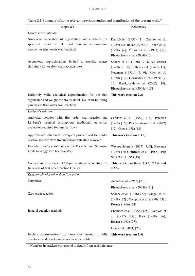
CHAPTER 2
52
Table 2.1:Summary of some relevant previous studies and contribution of the present work.*
Approach References
Graetz series solution
Numerical calculation of eigenvalues and constants for
specified values of Da and common cross-section
geometries (first order wall reaction)
Damköhler (1937) [1]; Carslaw et al.
(1959) [2]; Bauer (1976) [3]; Shah et al.
(1978) [4]; Özisik et al. (1982) [5] ;
Bhattacharya et al. (2004b) [6]
Asymptotic approximations limited to specific ranges
(infinitely fast or slow wall reaction rate)
Sellars et al. (1956) [7, 8, 9]; Brown
(1960) [7, 10]; Solbrig et al. (1967) [11];
Newman (1973a) [7, 9]; Kays et al.
(1980) [12]; Housiadas et al. (1999) [7,
13]; Balakotaiah et al. (2002) [14];
Bhattacharya et al. (2004a) [15]
Uniformly valid analytical approximation for the first
eigenvalue and weight for any value of Da with no fitting
parameters (first order wall reaction)
This work (section 2.2)
Lévêque’s solution
Analytical solution with first order wall reaction and
Lévêque’s original assumptions (additional numerical
evaluation required for laminar flow)
Carslaw et al. (1959) [16]; Petersen
(1965) [16]; Pancharatnam et al. (1972)
[17]; Ghez (1978) [18]
Approximate solution to Lévêque’s problem and first-order
reaction kinetics with no numerical evaluation involved
This work (section 2.3.2)
Extended Lévêque solutions in the Dirichlet and Neumann
limits (analogy with heat transfer)
Worsoe-Schmidt (1967) [7, 8]; Newman
(1969) [7]; Gottifredi et al. (1985) [19];
Shih et al. (1995) [19]
Corrections to extended Lévêque solutions accounting for
finiteness of first order reaction kinetics
This work (sections 2.3.3, 2.3.4 and
2.3.5)
Reaction kinetics other than first-order
Numerical Acrivos et al. (1957) [20] ;
Bhattacharya et al. (2004b) [21]
Zero-order reaction Sellars et al. (1956) [22] ; Siegel et al.
(1958) [22] ; Compton et al. (1990) [23] ;
Rosner (1966) [24]
Integral equation methods Chambré et al. (1956) [25] ; Acrivos et
al. (1957) [25] ; Katz (1959) [26];
Rosner (1963) [27];
Grau et al. (2001) [28]
Explicit approximations for power-law kinetics in fully
developed and developing concentration profile
This work (section 2.4)
* Numbers in brackets correspond to details from each reference.

MASS TRANSFER IN A MICROCHANNEL: FINITE REACTION RATES & KINETIC NORMALIZATION
53
Table 2.1 (continued): Additional details concerning each reference
[1] Report of the first 3 terms in Graetz series for plug-flow in a circular channel with 0.1Da = , 1, 10
and 100 and a plot from where the first 3 eigenvalues can be estimated for 30.1 10Da< < . See
also Paneth et al. (1931).
[2] First 6 eigenvalues for plug-flow in circular or planar duct for several values of Da .
[3] First 11 eigenvalues for a parallel plates conduit with homogeneous and heterogeneous first-order
reactions (for 0Da = , 0.1, 1, 10 and 100) in laminar flow.
[4] Review of several works in the field of heat transfer with finite wall thermal resistance.
[5] First 12 eigenvalues for laminar flow inside a circular tube for 0Da = , 0.1, 1, 10 and 100, as well
as the quantities needed to obtain the first twelve weights n
w .
[6] First 5 eigenvalues and weights for 0.01Da = , 0.1 , 1, 10 and 100 in channels with common
cross-section shapes (circular, plates, square and equilateral triangle). They also plot 1λ and 1w as
a function of Da for plug and laminar flows ( 3 210 10Da−
< < ).
[7] Constant wall temperature (Dirichlet) conditions (heat transfer analogy for the case of infinitely
fast reactions).
[8] Constant wall flux (Neumann) condition (heat transfer analogy for the case of slow reactions).
[9] Asymptotic formulas for higher eigenvalues and constants. Some obtained with the Wentzel-
Kramers-Brillouin (WKB) method. See Bender et al. (1978) for more details.
[10] Numerical calculation.
[11] Higher eigenvalues through implicit expression which requires numerical evaluation for finite Da .
[12] Numerical results for uniform temperature and heat flux at the wall of channels with several cross-
sectional geometries.
[13] Extended Lévêque-type solutions for integration constants and eigenfunction derivatives at the
wall.
[14] First five eigenvalues and weights tabulated for Da = ∞ and circular, planar, triangular and square
geometries.
[15] Taylor expansions of the first eigenvalue for the kinetic regime ( 0Da → ), corresponding to the
situations of plug and laminar flow inside planar and circular ducts.
[16] Solution with Laplace transform for plug-flow conditions.
[17] Inversion of Laplace transformed solution in terms of an infinite summation with coefficients given
by recurrence relations (first 24 out of 50 coefficients are tabulated). Laminar flow conditions.
[18] Analytical solution using Laplace transform for the case of first-order reversible reaction.
Asymptotic expansions in the limits of fast and slow reactions are also presented.
[19] Heat transfer in non-newtonian fluids with constant wall temperature boundary condition.
[20] Numerical solution of an integral equation for the following reaction schemes: reversible first
order, consecutive first-order and irreversible second-order.
[21] Numerical results for power law kinetics (of orders 1 2m = , 1 and 2) for plug flow in a short
channel and also for some types of Langmuir-Hinshelwood kinetics, including parameter ranges
where the solution exhibited multiplicity behavior.
[22] Graetz solution with uniform axial heat flux by the eigenfunction expansion method.

CHAPTER 2
54
Table 2.1 (continued): Additional details concerning each reference
[23] Analytical solution in Laplace’s domain to the problem of mass transfer in a channel cell-crystal-
electrode system with zero-order reaction, under Lévêque’s assumptions.
[24] Solutions to the wall concentration profile, for several classes of boundary layer problems, given by
0~ 1wall
c z z− for 0z z< .
[25] General solution to a class of laminar boundary layer-type flow fields past solid surfaces where
catalytic reactions with arbitrary mechanisms take place. This resulted in a nonlinear Volterra
integral equation from where the surface reaction rate can be calculated once the concentration
distribution at the wall is known (measured). For first-order reaction, the equation can be solved for
certain geometries in terms of a convergent infinite series.
[26] Considers fully developed laminar flow in a circular tube and from an integral equation, surface
concentration can be calculated from the reaction rate (which can be known from the cross-section
average concentration). The usefulness of this approach for kinetic studies and reactor design was
also discussed for arbitrary reaction rates.
[27] Solutions in a catalytic flat plate for uniform approaching velocity were obtained for power-law
kinetics at the surface in the form ( )wallz f c= .
[28] Transformation of the original PDE problem with reactions of arbitrary kinetics into a system of
integral equations using a Green’s function combined with generalized Fourier expansions. The
kernels of the integral operators are related to an eigenvalue problem (with homogeneous kinetic-
independent boundary conditions). Expressions in the slow, fast and instantaneous reaction regimes
were considered to improve the performance of the numerical solution of the resulting integral
equations.
Figure 2.1: Schematic representation of the concentration profile in the channel domain
showing the two main mass transfer regimes considered in this work.
L
a
plug or laminar flow0
r
z
u
( )u r
( ),c r z
z = 1
porous catalytic
coating
r =1; R = 0
R δ
developing profile fully developed profile
MASS TRANSFER IN A MICROCHANNEL: FINITE REACTION RATES & KINETIC NORMALIZATION
55
2.2.1 Theoretical background
We consider straight parallel plate or circular channels with uniform cross-sectional area, in
isothermal steady-state operation, coupled with a first-order heterogeneous reaction in a porous
catalytic coating with uniform properties (Figure 2.1). Under these assumptions, the convective
diffusion equation is (Deen 1998; Bird et al. 2002)
( )
2 22
2 2 m
c c cPe v x
x z zα α
∂ ∂ ∂+ =
∂ ∂ ∂ for parallel plates, and (2.1a)
( )
22
2
1m
c c cr Pe v r
r r r z zα α
∂ ∂ ∂ ∂+ =
∂ ∂ ∂ ∂ for a circular channel (2.1b)
where the dimensionless independent variables are the axial position scaled by the channel
length ( )ˆz z L= and the transverse position within the open channel (normalized by channel
radius ( )ˆr r a= or half-spacing between plates ( )ˆx x a= ). The concentration in this domain is
written as a fraction of the inlet concentration ( )ˆin
c c c= . The dimensionless uniform and
parabolic velocity profiles are
( )( ) ( )
231 laminar flow
21 plug-flow
Su r r
v ru
+−
= =
(2.2)
where 0S = for parallel plates, 1S = for circular channel and ( ) ( )v x v r= .
In Eqs.(2.1) two dimensionless parameters arise: the transverse mass Peclet number
( m
Pe u a D= ) and the channel aspect ratio ( a Lα = ). Axial diffusion is negligible up to
( )2
O α , i.e. for small aspect ratio channels. In this case ( 1α << ), the inlet Danckwerts’
boundary condition is simplified to uniform inlet concentration for m
Pe α>> ,
( ),0 1c r = . (2.3)
Despite the fact that the two domains (channel and catalytic layer) are coupled, a common
approach is averaging the latter by using the effectiveness factor (η ) concept. It has been
pointed out (Keyser et al. 1991; Bhattacharya et al. 2004b; Hayes et al. 2004) that for a first-
order reaction, the flux continuity requirement writes as a finite wall resistance (Robin-type)
boundary condition, even when internal diffusion inside the porous coating must be considered.
It can thus be written as
( )1
1,r
cDa c z
r=
∂= −
∂, (2.4)
CHAPTER 2
56
where the rescaled Damköhler number ( * II
RDa Da η δ= ), accounting for the concentration
boundary layer thickness ( ~ 1R
δ in the Graetz regime) could have been used instead. Here, the
Damköhler number compares the surface reaction timescale with the transverse diffusion one
( II
surfDa a k D= ). In terms of the observed reaction kinetics, Da writes as II
Da η . Uniform
wall flux (Neumann) and uniform wall concentration (Dirichlet-type) boundary conditions are
obtained for 1Da << and 1Da >> , respectively.
The well-known solution (Graetz 1883; Damköhler 1937) to this problem has the following
separable form:
( ) ( )
2
1 ,max
, exp n
n n
n m
zc r z A r
Pe
λϕ
α
∞
=
−=
∑ (2.5)
where ( )nrϕ is an eigenfunction in the transverse coordinate ( r or x ), while the exponential
term represents the axial dependence of the concentration profile (being ,maxmPe the transverse
Peclet number evaluated at the maximum velocity in the channel). Both transverse and axial
contributions are associated with n
λ , the thn eigenvalue (a function of Da , in general), which
satisfies Eq.(2.4). The typical dependence of the first eigenvalue on Da is illustrated in Figure
2.2 (full lines correspond to numerical calculations). Two asymptotes are of interest,
corresponding to low and high values of Da . For the former, the leading-order behaviour of the
first eigenvalue is
( )2 2
1 ~ Da O Daλ σ + as 0Da → , (2.6)
where ( ) max1S u uσ = + ( 0S = or 1 for parallel plates or circular channel, respectively).
On the other hand, near the Dirichlet limit ( 1Da >> ), the first eigenvalue does not change
significantly with Da . Carslaw et al. (1959) and Brown (1960) calculated these values as
22
1,
parallel plates4
circular channel5.783
πλ
∞
=
for plug-flow, and (2.7a)
21,
2.828 parallel plates
circular channel7.313λ
∞
=
for laminar flow. (2.7b)
Finally, n
A is the thn integration constant, which can be calculated from the orthogonality
condition (e.g. Townsend (1900), Bauer (1976)). The previous results are needed when
calculating the mixing-cup concentration:
( )
( ) ( )
( )
,A
A
u r c r z d A
c zu r d A
=
∫
∫. (2.8)
MASS TRANSFER IN A MICROCHANNEL: FINITE REACTION RATES & KINETIC NORMALIZATION
57
This is related to the conversion of reactant along the channel (with respect to the inlet
concentration), ( )1R
X c z= − . Substituting solution (2.5) into Eq.(2.8) leads to
( )
2
1 ,max
exp n
n
n m
zc z w
Pe
λ
α
∞
=
−=
∑ (2.9)
where n
w are dependent only on Da for each channel geometry and flow profile, and are called
in some references (Bhattacharya et al. 2004b) as the normalized Fourier weights, or are
presented as a combination of integration constants and eigenfunctions derivatives at the wall.
The lowest value of 1w appears in the Dirichlet limit ( 1,w∞
) and is given for plug-flow
conditions by(Balakotaiah et al. 2002)
2, ,2
n nw λ
∞ ∞= , parallel plates (2.10a)
2, ,4
n nw λ
∞ ∞= , circular channel. (2.10b)
In the next section, we use WKB results (Sellars et al. 1956) to write ,nw
∞ for laminar flow.
More details on the method developed by Wentzel, Kramers and Brillouin (WKB) can be found
in Bender et al. (1978). Frequently (Solbrig et al. 1967; Rice et al. 1995; Schmidt 1998; Belfiore
2003; Bhattacharya et al. 2004b), the calculation of ( )c z is simplified by retaining just one
term in Eq.(2.9), leading to
( )
21
1,max
~ expm
zc z w
Pe
λ
α
−
. (2.11)
2.2.2 Approximation to the eigenvalues
The calculation of conversion using (2.11) can be done once approximate dependences for 21λ
and 1w on Da are provided. In this section, we will be concerned with the first eigenvalue.
An improved estimate for 1λ for large Da is obtained here in an iterative manner, starting with
the result in the Dirichlet limit as a first guess, (0)1 1,λ λ
∞= . In this case, an approximation for
high eigenvalues but 1 1Da λ >> can be useful to characterise how 1λ approaches 1,λ∞
in an
intermediate range of Da . For plug-flow between parallel plates, Robin’s boundary condition
can be expanded for large 1Da λ as ( )(0)
1 1 1 1arctan ~ ...Da Daλ λ λ λ= − + . Assuming that it
is sufficient to retain these terms in the expansion, the improved result writes as
1 1,~1
Da
Daλ λ
∞
+ (2.12)
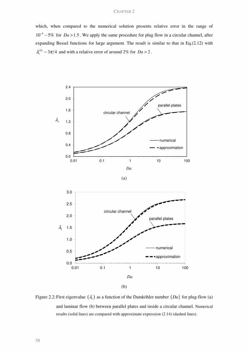
CHAPTER 2
58
which, when compared to the numerical solution presents relative error in the range of
410 5%−− for 1.5Da > . We apply the same procedure for plug flow in a circular channel, after
expanding Bessel functions for large argument. The result is similar to that in Eq.(2.12) with
(0)1 ~ 3 4λ π and with a relative error of around 2% for 2Da > .
(a)
(b)
Figure 2.2: First eigenvalue ( )1λ as a function of the Damköhler number ( )Da for plug-flow (a)
and laminar flow (b) between parallel plates and inside a circular channel. Numerical
results (solid lines) are compared with approximate expression (2.14) (dashed lines).
0.0
0.4
0.8
1.2
1.6
2.0
2.4
0.01 0.1 1 10 100
numerical
approximation
circular channel
parallel plates
1λ
Da
0.0
0.5
1.0
1.5
2.0
2.5
3.0
0.01 0.1 1 10 100
numerical
approximation
circular channel
parallel plates
1λ
Da

MASS TRANSFER IN A MICROCHANNEL: FINITE REACTION RATES & KINETIC NORMALIZATION
59
For laminar flows, we expand hypergeometric functions in ( )xϕ or ( )rϕ for large eigenvalues
(Abramowitz et al. 1972) leading to the following form of Robin’s condition:
11 1
1tan
2
Daλ
λ λ= + (for parallel plates) (2.13a)
11
tan4
Daπλ
λ
− =
(for circular channel) (2.13b)
For large 1Da λ , the expansion of ( )arctan x for large argument in Eqs.(2.13) leads to a
rational function, which can be corrected to the right Dirichlet limit, yielding a relationship like
Eq.(2.12). This result improves the estimate of the eigenvalues for 1Da > .
2.2.2.a Uniformly valid approximation (all values of Da )
The previous results show that: (a) two asymptotic regions exist, where the eigenvalues are well
characterized; and (b) the transition from the ~ 1Da region to the Dirichlet limit is well
described by a rational function. An approximate expression of the same form of Eq.(2.12) can
be easily conceived using asymptotic methods (e.g. Gottifredi et al.(1986)), so that both limits
are fulfilled:
21 2
1,
~1
Da
Da
σλ
σ λ∞
+ (2.14)
Eq.(2.14) has higher relative error (compared to numerical results) in the range of ~ 2 3Da − ,
which is less than 2.5% or 4% for plug-flow between parallel plates and circular channel,
respectively. For laminar flows, the first eigenvalue is predicted with errors just slightly above
1% and 2% for plates and round tube. The numerical results and Eq.(2.14) predictions are
plotted in Figure 2.2. Expressions for this type have been also sought in other contexts
(Villermaux 1971; Houzelot et al. 1977; Haji-Sheikh et al. 2009), but the final dependence on
Da results in much more complicated expressions or are the product of fitting procedures (with
numerically evaluated coefficients). Eq.(2.14) gives an extremely simple functional dependence,
while retaining the asymptotically correct behaviour.
We note that previous literature is full of procedures for calculation of eigenvalues and weights
(or related quantities), due to the high importance of estimating conversion (alternatively,
mixing-cup temperature) or Sherwood (and Nusselt) numbers. Table 2.1 provides a short list of
some relevant studies concerning the calculation of eigenvalues for Graetz series’ terms with
first-order wall reaction (more examples could be found in Shah and London (1978) or other
textbooks). We distinguish between two approaches.

CHAPTER 2
60
First, and probably more ubiquitous, examples of numerical calculation for specified values of
Da are presented. Secondly, explicit analytical approximations exist but are of extremely
limited application, namely high eigenvalues ( 1n >> ) asymptotics in the Dirichlet/Neumann
limit, where for example the effect of finite kinetics on the first (lowest) eigenvalue is ignored
(see Table 2.1).
The asymptotically correct correlation (2.14) we propose works very reasonably in the
intermediate range of ~ 1Da . This expression is also attractive when optimal parameter regions
are being searched, avoiding extensive numerical evaluation. Moreover, the effects of geometry
and flow profile are indicated explicitly.
2.2.3 Approximation to n
w coefficients
Combining Robin’s boundary equation with the orthogonality condition, we can obtain a
compact result for the integration constant given by
( )
12
1n
n n n
Da d DaA
dλ ϕ λ
−
=
. (2.15)
Therefore, when Da is finite ( ~ 1 ), we use Eq.(2.15) to obtain
( )
( )
2
~1
n
n
dw
d Da
σ λ (2.16)
The typical dependence of the first Fourier weight (which is also the largest one) on Da is
represented by a smooth transition between two asymptotic plateaus in the limits of 0Da →
and Da → ∞ . The variation in the intermediate range of Damköhler number is not easily
obtained and extending the asymptotic expansions in the limits is beneficial for small and large
(finite) Da , but unreasonable when ~ 1Da .
When 1Da << , the first Fourier weight is directly obtained from Eq.(2.16), once we know that
the first eigenvalue in this limit is described by Eq.(2.6). Thus,
( ) ( )2
1 0 1w Da O Da→ = − . (2.17)
The Dirichlet limit for plug-flow can be found in Eqs.(2.10). For fully developed parabolic flow
profile, we follow the WKB method (Sellars et al. 1956) to obtain
( )
( )
5/6
7/3 7/3, , ,
12 33.0384
1 6n n n
w λ λπ
− −
∞ ∞ ∞= =
Γ parallel plates (2.18a)
MASS TRANSFER IN A MICROCHANNEL: FINITE REACTION RATES & KINETIC NORMALIZATION
61
( )
( )
5/6
7/3 7/3, , ,
32 38.1023
1 6n n n
w λ λπ
− −
∞ ∞ ∞= =
Γ circular channel. (2.18b)
Even though Eqs.(2.18) were conceived for large eigenvalues (thus, large n ), the results for
1,w∞
with the appropriate first eigenvalues (Eqs.(2.7)) are in good agreement with numerical
solutions for parallel plates ( 1, 0.9104w∞
= ) and for circular channel ( 1, 0.8191w∞
= ), with
maximum relative errors of 1.3% and 0.3%, respectively.
As we saw previously, eigenvalues approach their Dirichlet values 1,λ∞
according to Eq.(2.12).
This is general for the geometries and flow profiles studied, but more accurate for plug-flow,
where the Fourier weight tends to its limit value 1,w∞
, as
1 21,
2 11w
Da
σ
λ∞
= +
.
We can then say generically that,
( )1 1,
11w Da w
Da∞
→ ∞ = +
(2.19)
represents the correct trend in this asymptotic limit. Eq.(2.19) gives less than 5% relative error
in the following ranges: 6Da ≥ (plug-flow between plates); 3Da ≥ (plug-flow inside a circular
channel); 15Da ≥ (laminar flow between plates); and 8Da ≥ (laminar flow inside circular
duct).
2.2.3.a Uniformly valid approximation (all values of Da )
As expected, the transition from the low- Da asymptote ( 1 1w → ) to the high- Da asymptote
( 1 1,w w∞
→ ) in the intermediate region of ~ 1Da is not satisfactorily described by these limits.
Table 2.2 contains the asymptotic values 1,w∞
for the geometries and flow profiles studied. Both
bounds on 1w ( 1 1w = and 1 1,w w∞
= ) work as approximations outside the intermediate range of
Da ,
max
11, min
1,~
,
Da Daw
w Da Da∞
≤
≥ (2.20)
Values of minDa and maxDa are given in Table 2.2 for maximum relative errors of the first
weight, as given by Eq.(2.20), of around 5% and 1%. We can see that when ~ 1Da , no
satisfactory approximation is obtained.

CHAPTER 2
62
Table 2.2: Range of Da in which 1w can be approximated by either
1 1w = ( )maxDa Da< or 1 1,w w∞
= ( )minDa Da> .
error 5%< error 1%<
1,w∞
maxDa minDa maxDa minDa
plug flow plates 0.8106 2.5 17 0.8 100
circular 0.6917 2.1 36 0.7 200
laminar
flow
plates 0.9104 5.1 4.1 1.0 34
circular 0.8191 2.1 12 0.6 70
Note that we have more information when Da is high: the non-leading order variation is of
( )1
O Da− , while the first Fourier weight deviates very slowly ( ( )
2O Da ) from 1 as 1Da →
from 0). Therefore, we construct a uniformly valid approximation from Eq.(2.19):
( )
1 1, 1,
1, 1,
1
1 1
w w w
w Daw
∞ ∞
∞ ∞
−=
− − as Da → ∞ .
A simple expression that also allows the small Da limit to be fulfilled writes as
1 1,
1,1,
1,
111
1
w w
wwDa
w
∞
∞∞
∞
−=
−−+
(2.21)
where 1,w∞
is obtained by previously given expressions (independent of Da ). Of course
Eq.(2.21) is only a particular case of the general empirical equation proposed by Churchill and
Usagi (1974) to successfully correlate experimental and numerical data for a wide range of
problems (e.g. determination of Sherwood and Nusselt numbers as a function of the Damköhler
number for triangular channels (Groppi et al. 1997)). Though a wide variety of problems
involving functions that approach constant values in both limits have been successfully dealt by
this kind of expressions, to the authors’ knowledge it so far has not been applied to the
prediction of 1w as a function of Da in two-dimensional models.
Eq.(2.21) can be generalized to a powered addition of asymptotic limits (Churchill et al. 1974),
which results in introducing an extra parameter into the correlation
1
1 1, 1,
1, 1,
11
1
bb
w w wDa
w w
−
∞ ∞
∞ ∞
− − = + −
. (2.22)
MASS TRANSFER IN A MICROCHANNEL: FINITE REACTION RATES & KINETIC NORMALIZATION
63
The simplest form to determine b is to ask for the correlation to produce the correct result when
the right-hand side of Eq.(2.22) is 2, i.e. when ( )1, 1,1Da w w∞ ∞
= − . In that case, 1b ≈ for plug
flow between parallel plates and for laminar flow (circular and slit ducts), but 4b ≈ when plug-
flow in a circular channel is being studied. However, the numerical results are still well
approximated by (2.22) when b changes around these values.
The correlation given by Eq.(2.21) predicts numerical results for parallel plates with 2.5%
maximum error for plug-flow (at ~ 2Da ), and 2% error for laminar flow (around ~ 8Da ). For
plug-flow inside a circular channel, Eq.(2.22) with 4b ≈ gives less than 6% relative error near
~ 7Da (and about 10% had we considered 1b ≈ ). For laminar flow inside a round tube, only
1.4% maximum error is observed near ~ 1Da .
2.2.4 One-term approximation for the mixing-cup concentration
The prediction of the exit mixing-cup concentration from Eq.(2.11) (with 1w from Eq.(2.22) and
the first eigenvalue from Eq.(2.14)) is compared with numerical solution of Eqs.(2.1) in Figure
2.3, where the quality of our approximations for the quantities involved in Eq.(2.11) is tested.
We also plot the results in a parametric range where the one-term approximation is expected to
fail (large m
Peα ). The range of ( )*m m
Pe Peα α< where Eq.(2.11) is applicable is identified
for the first time for several representative values of Da , as are the magnitudes of error
involved.
For ( )~ 1m
Pe Oα , the error associated with the approximation is in the range of error involved
in the estimation of eigenvalues and Fourier weights. When m
Peα increases, retaining just one
term in Eq.(2.9) is not sufficient (the convection-dominated regime in section 2.3 will be
appropriate for this limit). This is particularly noticeable at high Da , for example in the case of
plug-flow between parallel plates (Figure 2.3a), where error increases from 4% to 11% at
100m
Peα = , when Da changes from 1 to 410 . Moreover, in the same situation, less than 5%
relative error (in the range of meaningful absolute values for concentration) is obtained only for
20m
Peα < when 10Da = or 410Da = . The external mass transfer controlled limit is,
therefore, the one where convection-dominated solutions are more relevant, due to the existence
of a concentration boundary layer.

CHAPTER 2
64
(a) Plug flow between parallel plates
(b) Plug flow inside a circular channel
Figure 2.3: Exit mixing-cup conversion as a function of m
Peα for the channel geometries and
flow profiles studied. Curves for several values of IIDa Da η= are plotted, comparing
numerical results (full lines) with approximate 1-term expression (Eq.(2.11), dashed lines).
0
0.1
0.2
0.3
0.4
0.5
0.6
0.7
0.8
0.9
1
0.01 0.1 1 10 100
numerical
approximation
( )1c z =
mPeα
1=
10=
410=
0 1.Da =
0.0
0.1
0.2
0.3
0.4
0.5
0.6
0.7
0.8
0.9
1.0
0.01 0.1 1 10 100
numerical
approximation
( )1c z =
mPeα
1=
10=
410=
0 1.Da =

MASS TRANSFER IN A MICROCHANNEL: FINITE REACTION RATES & KINETIC NORMALIZATION
65
The same remark can be made when plug-flow in a circular tube is considered (Figure 2.3b).
The maximum relative errors occur at high m
Peα and Da (around 18% for 10Da = and 410 ,
but only 0.2% when 1Da = , at 100m
Peα = ). Maximum of 5% relative error is obtained for
10m
Peα < when 10Da = or 410 .
For laminar flows (Figure 2.3c and d), the same observations hold in the high Da region: error
increases significantly with m
Peα and curvature (maximum errors of 6% in parallel plates and
12% in circular channel, for 100m
Peα = and 410Da = ). The range over which is possible to
apply the one-term approximation also gets narrower for circular channel (less than 5% error
obtained for 30m
Peα < when 10Da = , and 20m
Peα < when 410Da = ), while parallel plates
can be represented correctly at least up to 100m
Peα = with less than 5% error for 10Da ≤ but
only up to 70m
Peα = , close to the Dirichlet limit ( 410Da = ).
The introduction of the results for 1w and 1λ presented in previous sections into (2.11) allow us
to calculate conversion in a channel directly from the governing dimensionless parameters.
However, if explicit approximations to conversion are sought (without going through the
eigenvalue and weights dependence relationships), simple expressions for kinetic control
conditions and mass transfer controlled conditions can provide useful insight. While in the
former case, this yields the well-known result for exponential decrease in the equivalent
homogeneous model (e.g. Damköhler (1937)):
( )( )1
~ expm
S Da zc z
Peα
− +
( 1Da << ), (2.23)
for the latter, we obtain
( )( )
2 41, 1,
1, 2 2,max
11 1~ exp 1 1
m m
z zSc z w O
Pe Da Pe Da
λ λ
α σ α
∞ ∞
∞
− + + + +
( 1Da >> ). (2.24)
Eq.(2.24) with an ( )1O Da correction to Dirichlet’s limit agrees reasonably well with the
numerically calculated data from gPROMS®. For instance, for laminar flow in a circular
channel and 20Da = , Eq.(2.24) gives less than 44 10−× absolute error for 1
mPe zα < . For
mPe zα around 1 and up to 20, the approximation predicts less than 2% error. For 10Da = ,
the relative error is near 2% when ~ 1m
Pe zα . In the same conditions, maximum error is
around 5% for all m
Pe zα higher than 0.65. For 0.65m
Pe zα < , the high relative errors
correspond to maximum absolute error of 45 10−× , since concentration is getting negligible on
this limit.
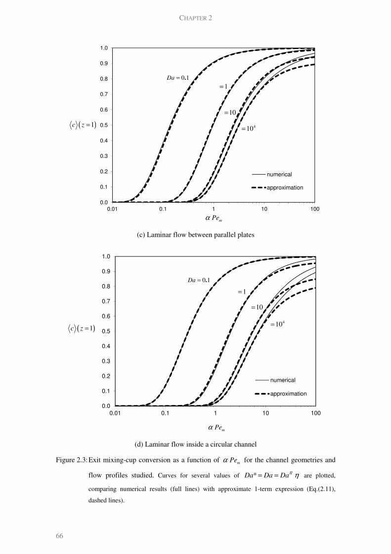
CHAPTER 2
66
(c) Laminar flow between parallel plates
(d) Laminar flow inside a circular channel
Figure 2.3: Exit mixing-cup conversion as a function of m
Peα for the channel geometries and
flow profiles studied. Curves for several values of * IIDa Da Da η= = are plotted,
comparing numerical results (full lines) with approximate 1-term expression (Eq.(2.11),
dashed lines).
0.0
0.1
0.2
0.3
0.4
0.5
0.6
0.7
0.8
0.9
1.0
0.01 0.1 1 10 100
numerical
approximation
( )1c z =
mPeα
1=
10=
410=
0 1.Da =
0.0
0.1
0.2
0.3
0.4
0.5
0.6
0.7
0.8
0.9
1.0
0.01 0.1 1 10 100
numerical
approximation
( )1c z =
mPeα
1=
10=
410=
0 1.Da =

MASS TRANSFER IN A MICROCHANNEL: FINITE REACTION RATES & KINETIC NORMALIZATION
67
Eq.(2.11) with our approximations for 1λ and 1w , and in particular limits (2.23) and (2.24),
show the dependence of conversion on the Graetz parameter (the reciprocal of m
z Peα ) and on
Da , for finite kinetic rates (tending to kinetic and mass transfer controlled limits). Explicit
analytical expressions without the need of numerical evaluation for this case have not been
presented previously. Bhattacharya et al. (2004b) present explicit asymptotic expressions for
conversion for a parametric range of 1P >> (their parameter P is equivalent to ~m
Peα ) in the
Dirichlet ( Da → ∞ ) and Neumann ( 0Da → ) limits. The applicability of these results in the
range of ~ 1m
Pe zα is extremely limited (e.g. more than 20% relative error for 16m
Peα <
and 10Da = in round tube with parabolic flow). For a small aspect ratio channel, this merely
rewrites Lévêque’s regime results, which have been dealt extensively elsewhere (Lévêque 1928;
Levich 1962; Cowherd Jr et al. 1965; Petersen 1965; Solbrig et al. 1967; Pancharatnam et al.
1972; Ghez 1978). Therefore, in terms of explicit approximate solutions, the results in this
section completes the description of this problem in previous literature, especially in what has
been identified (Bhattacharya et al. 2004b) as the parameter regime for the optimal design of
catalytic monoliths: ~ ~ 1m
P Peα (e.g. near the mass transfer controlled regime). Moreover, it
is possible to identify the effect of design variables on conversion from Eq.(2.11): (a) the
channel length L appears only in the argument of the exponential, showing a steeper increase in
conversion for longer channels; and (b) the pre-exponential factor is a decreasing function of the
channel transverse length a , but the dominant behavior is given by the increase of the time
constant for interphase mass transfer in the denominator of the exponential argument, lowering
conversion for channels with larger cross-sections. The influences of the fluid velocity inside
the channel and of the bulk diffusivity on conversion are reciprocal to those of L or a ,
respectively. Finally, both diffusivity and kinetic constants depend on the operating
temperature, the latter being usually more sensitive. Naturally, higher temperature leads to a
steeper decrease of the mixing-cup concentration, as a result of faster reaction.
The dependence of the parameters on the operation and design variables can be nonlinear (e.g.
exponential dependence of the kinetic constant on temperature) or appear in several terms of the
solution (e.g. the channel radius and bulk diffusivity appear in both Graetz and Damköhler
numbers), which complicates the analytical simplified analysis. However, under some
assumptions, it is possible to obtain further insight on the effect of physical variables on
conversion. When the 1-term Graetz series solution is acceptable, the channel length required to
achieve a conversion R
X at a specified fluid velocity u and constant physical properties is
given as a function of the channel radius a , kinetic parameters, geometry, flow profile and
temperature by
( )
( )
/2 /1, 01,max
2 /0 1, 1, 1, 0
1 11ln ln
1 1
E RTE RT
E RT
R
w Da ewa u eL
D Da X w w Da eσ λ
−
∞∞
−
∞ ∞ ∞
+ − = + + − + −
(2.25)
CHAPTER 2
68
Alternatively, the operation flow-rate can be calculated for a given channel length L , as a
function of e.g. temperature ( L and u can also be combined in the reactor’s residence time,
convτ ). This assumed a weak dependence of diffusivity on temperature compared to the one of
the kinetic constant, which is acceptable. Nevertheless, such dependence (as well as the
calculation of the effectiveness factor) can be included, and the result continues explicit for the
channel length or fluid velocity. Note that 0Da is de Damköhler number evaluated with the pre-
exponential factor (Da at zero activation energy). The values of σ , 21,λ
∞ and 1,w
∞ are known for
given flow profile and channel cross-section. Iso-conversion lines in a T u− operating
diagram can be drawn according to the above expression (in this case, for fully developed
profile conditions). As an example, consider: 100a mµ= , 5 210D m s−
= , 60 10Da = ,
410E R K= and specified conversion of 0.99R
X = . The following ( );conv
T τ operation points
should give a performance close to our target: ( )300º ;90C ms , ( )500º ;2C ms , ( )800º ;1.2C ms
and ( )1000º ;1.2C ms , for example. This was compared with numerical simulations in a matrix
of parameter values ( )convT τ× . The points given by the expression above predicted conversion
correctly with maximum of 0.15% of relative error. This line separates two sets of results: when
conversion is higher than specified and when conversion is lower than specified. It is obvious
that such numerical effort can be avoided: rigorous numerical solution can be restricted to
operating points around the given boundary (and not in the complete parametric space).
Another strategy that we explore next, is the use of Lévêque type corrections (constructed for
1m
Peα >> ) to improve the performance at intermediate values of ~ 1m
Peα . To our
knowledge, the effect of finite reaction rate conditions in these corrections has not been
discussed so far.
2.3 LÉVÊQUE’S REGIME (DOMINANT CONVECTION)
At high flow rates ( 1m
Peα >> ), the transport of reactant towards the walls is now limited by
transverse diffusion. If the consumption of reactant at the wall is fast enough, the solution can
be decomposed in the transverse direction into two domains: an outer region (which occupies
most part of the channel’s cross-section, 0 1r≤ < ) and a concentration boundary layer near
1r = . In this section, we treat the convection dominated regime as a perturbation problem,
allowing us to separate the influence of effects, such as curvature and nonlinearities in the
velocity profile, and identify the parametric conditions where they are relevant, under finite
reaction kinetics conditions. Table 2.1 summarizes some of the previous work invariably
associated with Dirichlet and Neumann boundary conditions.

MASS TRANSFER IN A MICROCHANNEL: FINITE REACTION RATES & KINETIC NORMALIZATION
69
2.3.1 Structure of the perturbation problem in Lévêque’s regime
In the presence of significant consumption of reactant (with an associated concentration drop,
( )~ 1c O∆ ), transverse (and axial) gradients are much larger than ( )1O and we stretch the
transverse variables in Eqs.(2.1) to obtain a correct rescaling:
( )
2 22 2 2
2 2X m X
c c cPe v X
X z zα δ α δ
∂ ∂ ∂+ =
∂ ∂ ∂ for parallel plates (2.26a)
( )
2 22 2 2
2 21R
R m R
R
c c c cPe v R
R R R z z
δα δ α δ
δ
∂ ∂ ∂ ∂− + =
∂ − ∂ ∂ ∂ for a circular channel. (2.26b)
The velocity profiles given by Eq.(2.2) become
( )3 1 laminar flow
2
1 plug-flow
X
X
XX
v X
δδ
−
=
and ( )4 1 laminar flow
2
1 plug-flow
R
R
RR
v R
δδ
−
=
where ( )1R
R r δ= − and ( )1X
X x δ= − are the transverse stretched spatial variables, and
, 1X R
δ δ << are the dimensionless thicknesses of the concentration boundary layer near the wall.
The only distinguished limit in Eqs.(2.26) reflects a convection-transverse diffusion dominance.
Balancing those two terms, the inner layer scales become: ( )1/2
~ ~R X m
Peδ δ α−
for plug flow
and ( )1/3
~ 3X m
Peδ α−
for laminar flow between parallel plates or ( )1/3
~ 4R m
Peδ α−
if a
parabolic velocity profile inside a circular channel is considered. We kept the axial diffusion
term in Eqs.(2.1) but near the wall its importance relative to transverse diffusion is ( )1
axO Pe
− for
plug-flows, while for laminar flows its effect only shows up at ( )2 3 2/3
axO Peα , which are
smaller than any other terms calculated next.
We can see the convection-dominated limit as a perturbation problem, where Lévêque’s
solution is nothing but the leading-order result. The inner problem given by Eqs.(2.26) can be
decomposed into subproblems once the dependent variable in this region is expanded as a series
in δ , i.e. at the boundary layer ( blc c≡ ):
( ) ( )0
, ; , n
m n
n
c R z Pe c R zα δ
∞
=
=∑ (2.27)
Since the flux continuity at the interface is explicitly free of the perturbation parameter, the
appropriate rescaled form for the ( )n
O δ subproblem is (replace R by X for parallel plates)
( )0
* 0,n
n
R
cDa c R z
R=
∂= =
∂ (2.28)

CHAPTER 2
70
Here however, *Da ( )II
RDa η δ= includes the correct length scale for the concentration
gradient (R
a δ ). For * ~ 1Da , Eq.(2.28) must retain its full structure, but Neumann and
Dirichlet conditions are natural limits for * 1Da << and * 1Da >> . Additional details on the
definition of regimes from *Da can be found in Chapter 4.
The inlet boundary condition is homogeneous ( ( ),0 0n
c R = ) for 1n ≥ and the general matching
procedure can be reduced in this case to Prandtl’s condition for 0n = :
( ) ( )0 , , 1outc R z c r z→ ∞ → = (finite), and (2.29a)
( ), 0n
c R z→ ∞ = for 1n ≥ . (2.29b)
Then, the composite solution is simply given by
( ) ( ) ( ), , ,out blc r z c r z c R z cp= + −
where ( ) ( )0lim , ,bl out
R
cp c R z c r z→∞
= = , and therefore the solution in the boundary layer is
uniformly valid over the complete transverse domain. At leading order, the simplified form of
the inner equations in the variables X or R becomes independent of the geometry (curvature
effects are of ( )RO δ and therefore neglected). Moreover, the laminar parabolic velocity profile
is linear up to ( )RO δ near the wall (Figure 2.1). This reproduces Lévêque’s analysis and
assumptions (Lévêque 1928).
2.3.2 Approximate solution to Lévêque’s problem under finite reaction rate conditions
From previous studies (see Table 2.1), it is clear (especially for laminar flow) that more
convenient solutions to the mixing-cup concentration without requiring numerical evaluation
are needed, when Da is finite. As shown in section 2.3.1, the correct scaling of Eq.(2.4)
includes the thickness of the boundary layer, which is the perturbation parameter in the
expansion given by Eq.(2.27). Thus, according to (2.8), the mixing-cup concentration profile is
also given by a perturbation series in powers of R
δ . In particular, each coefficient in
( )0
n
n
n
c z c δ
∞
=
=∑ (2.30a)
can be obtained from surface conditions from
( )( )
( )000
1 *1 0,
z
m
S Dac z c z d z
Peα δ
+= − ∫ , (2.30b)
( )( )
( )0
1 *0,
z
nn
m
S Dac z c z d z
Peα δ
+= − ∫ . (2.30c)
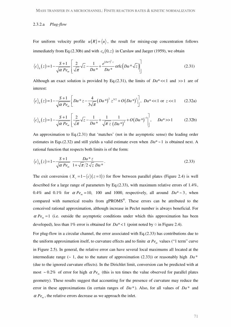
MASS TRANSFER IN A MICROCHANNEL: FINITE REACTION RATES & KINETIC NORMALIZATION
71
2.3.2.a Plug-flow
For uniform velocity profile ( )u R u= , the result for mixing-cup concentration follows
immediately from Eq.(2.30b) and with ( )0 0,c z in Carslaw and Jaeger (1959), we obtain
( )
( )
( )
2*
0
1 2 11 erfc *
* *
Da z
m
S ec z z Da z
Da DaPeα π
+= − − +
(2.31)
Although an exact solution is provided by Eq.(2.31), the limits of * 1Da << and 1>> are of
interest:
( ) ( ) ( )2 33/2
0
1 41 * * *
3m
Sc z Da z Da z O Da
Peα π
+ = − − +
, * 1Da << or 1z << (2.32a)
( )( )
( )3
20
1 2 1 1 11 *
* *m
Sc z z O Da
DaPe z Daα π π
− +
= − − + +
, * 1Da >> (2.32b)
An approximation to Eq.(2.31) that ‘matches’ (not in the asymptotic sense) the leading order
estimates in Eqs.(2.32) and still yields a valid estimate even when * ~ 1Da is obtained next. A
rational function that respects both limits is of the form:
( )0
1 *1
1 2 *m
S Da zc z
Pe z Daα π
+= −
+. (2.33)
The exit conversion ( ( )1 1c
X c z= − = ) for flow between parallel plates (Figure 2.4) is well
described for a large range of parameters by Eq.(2.33), with maximum relative errors of 1.4%,
0.4% and 0.1% for 10,m
Peα = 100 and 1000, respectively, all around * ~ 3Da , when
compared with numerical results from gPROMS®. These errors can be attributed to the
conceived rational approximation, although increase in Peclet number is always beneficial. For
1m
Peα = (i.e. outside the asymptotic conditions under which this approximation has been
developed), less than 1% error is obtained for * 1Da < (point noted by ○ in Figure 2.4).
For plug-flow in a circular channel, the error associated with Eq.(2.33) has contributions due to
the uniform approximation itself, to curvature effects and to finite m
Peα values (“1 term” curve
in Figure 2.5). In general, the relative error can have several local maximums all located at the
intermediate range (~ 1, due to the nature of approximation (2.33)) or reasonably high *Da
(due to the ignored curvature effects). In the Dirichlet limit, conversion can be predicted with at
most ~ 0.2% of error for high m
Peα (this is ten times the value observed for parallel plates
geometry). These results suggest that accounting for the presence of curvature may reduce the
error in these approximations (in certain ranges of *Da ). Also, for all values of *Da and
mPeα , the relative errors decrease as we approach the inlet.
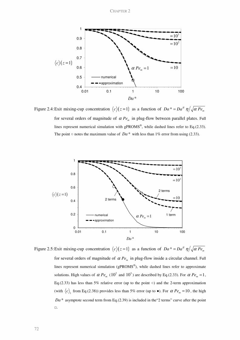
CHAPTER 2
72
Figure 2.4: Exit mixing-cup concentration ( )1c z = as a function of *DaII
mDa Peη α=
for several orders of magnitude of m
Peα in plug-flow between parallel plates. Full
lines represent numerical simulation with gPROMS®, while dashed lines refer to Eq.(2.33).
The point ○ notes the maximum value of *Da with less than 1% error from using (2.33).
Figure 2.5: Exit mixing-cup concentration ( )1c z = as a function of *DaII
mDa Peη α=
for several orders of magnitude of m
Peα in plug-flow inside a circular channel. Full
lines represent numerical simulation (gPROMS®), while dashed lines refer to approximate
solutions. High values of m
Peα ( 210 and 310 ) are described by Eq.(2.33). For 1m
Peα = ,
Eq.(2.33) has less than 5% relative error (up to the point ○) and the 2-term approximation
(with 1
c from Eq.(2.38)) provides less than 5% error (up to ●). For 10m
Peα = , the high
*Da asymptote second term from Eq.(2.39) is included in the“2 terms” curve after the point
□.
0.4
0.5
0.6
0.7
0.8
0.9
1
0.01 0.1 1 10 100
numerical
approximation
( )1c z =
1m
Peα = 10=
210=
310=
*Da
0
0.2
0.4
0.6
0.8
1
0.01 0.1 1 10 100
numerical
approximation
( )1c z =
1m
Peα =
10=
210=
310=
*Da
1 term
2 terms
2 terms

MASS TRANSFER IN A MICROCHANNEL: FINITE REACTION RATES & KINETIC NORMALIZATION
73
2.3.2.b Laminar flow
The degree of reactant’s conversion can be calculated from Eq.(2.30b) for both limits with the
asymptotic expressions for ( )0 0,c z presented in Ghez (1978), yielding
( )( ) ( ) ( )
2
4/3
0
1 * 1 *1 1.1521
m m
S Da S Dac z z z
Pe Peα δ α δ
+ += − + −
( ) ( ) ( )
3 4 25/31 * *
1.2506m m
S Da Da zz O
Pe Peα δ α δ
+ − +
for 1/3* 1Da z << , (2.34a)
and ( ) ( )( )2/3 1/3
0
11 0.8076 1 0.5952
*m m
Sz zc z S
Pe Da Peα δ α δ
+= − + + for 1/3* 1Da z >> . (2.34b)
where * IIDa Da η δ= and δ has different definitions according to the geometry and flow
profile (section 2.3.1). When compared with the numerical solution of the full model (from
gPROMS®), the ( )2*O Da and ( )
1*O Da− approximations (obtained truncating Eqs.(2.34) only
to leading-order dependence on z ) are rather limited in applicability, especially for a circular
channel geometry. However, we note that a rational expression (similar to Eq.(2.33)) bringing
together the solution for small and large values of *Da z , may actually perform better than (or
at least, comparably with) the individual limits it is meant to fulfill:
( ) 1/30
1 *1
1 1.2382 *m
S Da zc z
Pe Da zα δ
+= −
+ . (2.35)
Eq.(2.35) predicts conversion in a circular channel with around 1.4% error for 100m
Peα = and
~0.13% for 1000m
Peα = , as *Da increases. For slit channels though, the exit mixing-cup
conversion can be reasonably calculated over large parametric ranges (Figure 2.6). For example,
up to the Dirichlet limit (large *Da ) maximum relative errors are: 3% for 10m
Peα = , ~ 0.1%
for 100m
Peα = and ~ 0.01% for 1000m
Peα = . In this case, even when 1m
Peα = , less than
5% error is achieved for * 0.5Da < . The effect of curvature clearly reduces the accuracy of the
approximations (mainly for finite (moderate) values of m
Peα ), which stresses the importance
of a curvature correction.
2.3.3 Higher order corrections to Lévêque’s problem
The higher order problem accounting for curvature can be extracted from Eqs.(2.26) (plug-flow
profile) at ( )1/2
mO Peα
−
and is given by

CHAPTER 2
74
201 1
2
cc c
R z R
∂∂ ∂− =
∂ ∂ ∂ (2.36)
with boundary conditions for 1n = in Eqs.(2.29). The surface concentration value is calculated
inverting Laplace’s transform
( )
( )1 2
*0,
2 *
Dac R s
Da s s
= = −
+
.
The correction accounting for nonlinearity of the velocity profile at the boundary layer appears
at ( ) ( )1/3
~m
O O Peδ α−
and is calculated from
2 201 1
2 2
cc c XX
X z z
∂∂ ∂− = −
∂ ∂ ∂ at ( )
1/33
mO Peα
−
for parallel plates, and (2.37a)
2 20 01 1
2 2
c cc c RR
R z z R
∂ ∂∂ ∂− = − +
∂ ∂ ∂ ∂ at ( )
1/34
mO Peα
−
for a circular channel. (2.37b)
Eqs.(2.37) can be solved in Laplace’s domain and then inverted for high and low *Da .
2.3.4 Effect of curvature in a circular channel with plug flow
The results of interest are the limits of low and high *Da of the mixing-cup concentration
which according to Eq.(2.30c) are:
( )( )
( )
2 2 5/24
1
* 16* *
2 15m
Da z zc z Da O Da
Peα δ π
= − +
for * 1Da << (2.38)
( ) ( )2
1
4 11 *
*m
zc z O Da
Pe Dazα δ π
−
= − +
for * 1Da >> . (2.39)
From the previous numerical results, we saw that this correction is mainly needed for * 1Da >>
(note that for * 1Da << , the correction is of ( )2*O Da ). The “curvature correction” can be
simplified to ( )1~
m
zc z
Peα δ, only when * 1Da >> .
The high *Da asymptote in Eq.(2.39) improves the approximation even at moderate values of
this parameter (□ in Figure 2.5). In particular for * 100Da = , the error drops an order of
magnitude: from 27% to 1.5% ( 10m
Peα = ), from 1.29% to 0.02% ( 100m
Peα = ) and from
0.14% to 0.03% ( 310m
Peα = ). The low *Da term (Eq.(2.38)) is more useful for 1m
Peα = to
extend the validity of the approximate solution given by Eq.(2.33) from * 0.2Da < (limit shown
by ○) to * 0.5Da < (limit shown by ●), with maximum 5% relative error compared to numerical

MASS TRANSFER IN A MICROCHANNEL: FINITE REACTION RATES & KINETIC NORMALIZATION
75
results. The contribution of curvature 1
cδ is more significant at high *Da and is less than 1%
of 0
c for 100m
Pe zα ≥ , however it is less than 30% of 0
c for 10m
Pe zα ≥ .
2.3.5 Effect of nonlinear velocity profile in laminar flows
In this case, the higher order correction writes in the limits of high and low *Da as
( )( )
( ) ( )2 5/3 3
1
1~ 0.125 * *
m
Sc z Da z O Da
Peα δ
++ for * 1Da << (2.40)
( )( )
( )1/3
2
1
1 1.615~ 1 *
10 *m
S z zc z O Da
Pe Daα δ
−
−+
− +
for * 1Da >> . (2.41)
Again for low *Da , the contribution is of ( )( )2*
mO Da Peα δ and therefore negligible.
However, in the limit of high *Da , the correction is more significant.
2.3.5.a Parallel plates
Two terms in Eq.(2.41) should be retained in the ranges of 1.8 * 12Da< < , 4.4 * 20Da< < and
0.75 * 26.5Da< < for 10m
Peα = , 100 and 310 (with respective maximum relative errors of
0.20%, 0.03% and 0.009%, respectively). In particular for * 100Da = , errors are reduced by one
order of magnitude compared to the ones obtained with (2.35). For 10m
Peα = , ( )0
c z
reasonably describes numerical solutions up to * 12.7Da = (shown in Figure 2.6 by □).
2.3.5.b Circular channel
At low *Da , the improvement brought by Eq.(2.40) is not particularly visible, as for
1m
Peα = , the error is already less than 5% for 0.1Da* < (○ in Figure 7). Eqs.(2.40) and
(2.41 ) result in improvement of the rational function for 0
c (Eq.(2.35)) with transition
between asymptotes around * ~ 1Da . The effect of correction (2.41) at * 100Da = is quite
modest. When m
Peα is not high enough and *Da is large, the Graetz solution is more
appropriate to describe accurately the numerical results. In this case (finite m
Peα ), the
penetration of concentration gradients is visible at a length scale comparable to the channel
characteristic dimension a , much thicker than R
a δ .

CHAPTER 2
76
The leading order solution at low *Da , given by the first couple of terms in Eq.(2.34), can be
connected to Graetz’s estimate at the Dirichlet limit (Eq.(2.11)) with error slightly above 2% for
* 100Da = . Such approximation is plotted in Figure 2.7 for 10m
Peα = and writes as:
( )( )
( )
21,
1,,max
21,
1,,max
exp1 *
1 ~ 11 *
1 exp
m
m
m m
wPeS Da
cPe S Da
wPe Pe
λ
α
α δ λ
α δ α
∞
∞
∞
∞
−
+ −
−++ −
. (2.42)
As shown in Figure 2.4 to Figure 2.7 and in the previous discussion, the extended Lévêque
solutions improve the prediction of conversion significantly even at the exit of the channel.
Here, the flow can be already fully developed, so corrections due to velocity profile nonlinearity
are important. Improvement resulted for values of m
Peα as low as 10.
Figure 2.6: Exit mixing-cup concentration ( )1c z = as a function of *Da
( )1/3
3II
mDa Peη α= for several orders of magnitude of
mPeα for laminar flow
between parallel plates. Full lines represent numerical simulation with gPROMS®, while
dashed lines refer to approximate solutions. One-term solutions are given by Eq.(2.35).
Correction Eq.(2.41) is added to obtain the “2 terms” curve after □.
0.5
0.6
0.7
0.8
0.9
1
0.01 0.1 1 10 100
numerical
approximation
( )1c z =
1m
Peα =
10=
210=
310=
*Da
1 term
2 terms
1 term

MASS TRANSFER IN A MICROCHANNEL: FINITE REACTION RATES & KINETIC NORMALIZATION
77
Figure 2.7: Exit mixing-cup concentration ( )1c z = as a function of *Da
( )1/3
4II
mDa Peη α= for several orders of magnitude of
mPeα for laminar flow
inside a circular channel. Full lines represent numerical simulation (gPROMS®), while
dashed lines refer to approximate solutions. The correction in Eq.(2.41) is added to Eq.(2.35)
to obtain the “2 terms” curve. Eq.(2.42) is also plotted for 10m
Peα = .
2.4 KINETIC NORMALIZATION FOR ‘POWER-LAW’ REACTION RATES
When reactions are unimolecular or when all reactants (species i ) except one are present in
excess, ( ){ } ( ){ }1, 1,i
c r z c r z= = =R R . Moreover, if reactant concentration is kept in a
restricted range, the so-called ‘power-law kinetics’ can be used as a reasonable approximation to
the actual rate equation: ( ){ } ( )1, 1,m
surfc r z k c r z= = =R , where m is the order of reaction.
Concerning the coupled analysis of (channel) flow past a surface where a reaction with arbitrary
kinetics is occurring, a great deal of work exists (see Table 2.1). A generic approximate
approach to convective-transport problems past catalytic surfaces is to reduce the problem
(Lighthill transformation (1950)) to an integral equation relating surface concentration and
reaction rate (“integral equation method”), which is usually solved numerically.
Bhattacharya et al. (2004b) present numerical results for power law kinetics (of orders 1 2m = ,
1 and 2) for plug flow in a short monolith channel and also for some types of Langmuir-
Hinshelwood kinetics (with multiplicity behavior). They observed that the same asymptotes for
kinetic and mass transfer controlled limits were fulfilled.
0.4
0.5
0.6
0.7
0.8
0.9
1.0
0.01 0.1 1 10 100
numerical
approximation
210=
310=
( )1c z =
*Da
1m
Peα =
10=
1 term
2 terms
'matched' with Graetz

CHAPTER 2
78
In this section, we extend our approximations in fully developed Graetz and Lévêque’s regimes
to ‘power-law’ kinetics. Our objectives are the following: (a) to obtain explicit formulas for
conversion under kinetic and mass transfer control, and (b) to understand the influence of the
reaction rate law through calculation of higher-order contributions in suitable limits.
2.4.1 Developing concentration profile
When the concentration profile is developing, the rescaled wall boundary condition for the
nonlinear problem is:
( )0
* 0,m
R
cDa c R z
R=
∂= =
∂ (power-law kinetics) (2.43)
In Eq.(2.43), the *Da parameter is defined as usual in Lévêque’s regime with the thickness of
the boundary layer ( )II
RDa η δ= , however
surfk is replaced by ( )ˆ ˆ
surf in inc cR . To obtain
approximate solutions, we must reduce the boundary condition by choosing *Da (or its
reciprocal) as perturbation parameter ε . This will not result in any simplification of the
complete mass balance in the channel, which is free of ε . Therefore, we start by analyzing
Lévêque’s regime, where a set of assumptions for ( )~ 1q
R mPeδ α
−
<< ( 1 2q = for plug flow
and 1 3q = for laminar flow) allows simplification of the mass balance to Eqs.(2.26).
We consider a perturbation series for concentration of the following form
( ) ( ) ( )0
, ; ,n n
n
c R z c R zε δ ε
∞
=
=∑ (2.44)
where, ( ),n
c R z is the solution to the thn subproblem (of ( )n
O δ ), ε is the small parameter
(which can be either *Daε = for kinetic control or 1 *Daε = for mass transfer control) and
( )nδ ε are undetermined gauge functions of ε , which will be defined by convenient dominant
balances, obeying the following relation ( ) ( )1n nδ ε δ ε
+>> as 0ε → .
The subproblems appearing after introducing (2.44) into the leading-order problem from
Eq.(2.26) and collecting the same order terms are
2
2n n
c c
R z
∂ ∂=
∂ ∂ (plug flow) (2.45a)
2
2n n
c cR
R z
∂ ∂=
∂ ∂ (laminar flow). (2.45b)

MASS TRANSFER IN A MICROCHANNEL: FINITE REACTION RATES & KINETIC NORMALIZATION
79
Since our perturbation to boundary condition (2.43), associated with the nonlinear kinetics, will
render the problem linear, Eqs.(2.45) are amenable to be treated with Laplace transform of
( ) ( ) ( ), , ,0n n n
u R z c R z c R= − with respect to z , yielding the following general solutions for the
thn subproblem
( ), R s
nu R s const e
−= (plug flow) (2.46a)
( ) ( )1 3, Ai
nu R s const R s= (laminar flow). (2.46b)
Note that ( ),0 1n
c R = for 0n = but ( ),0 0n
c R = for 1n ≥ , and therefore ( ) ( ), ,n n
u R s c R s=
(for 1n ≥ ). Solutions (2.46) were obtained so that boundedness as R → ∞ is achieved.
The mixing-cup can be written as
( )( )
( )0
11
nn
nm
Sc z c
Peδ ε
α δ
∞
=
+= − ∑ , (2.47)
where the contributions from the ( )nO δ subproblems are
( )1
0 0 0
1z
n n
n
R R
c d cc z d z
R s d R
−
= =
∂ = =
∂ ∫ L . (2.48)
2.4.1.a Kinetically controlled regime
If we seek for a perturbation solution in *Daε = , the wall boundary condition (2.43) after
introduction of Eq.(2.44) becomes,
( )0 00
0,m
n
n n n
n nR
cc z
Rδ ε δ
∞ ∞
= ==
∂ =
∂ ∑ ∑ (power law kinetics) (2.49)
Since both wall concentration and flux are correctly scaled, the left-hand side (LHS) of (2.49) is
dominant and therefore the leading order term is unbalanced by any term in the right hand side
(RHS) as 0ε → , i.e.
( )0
0
0
0R
c
Rδ ε
=
∂=
∂ from where 0
0
0R
c
R=
∂=
∂ (2.50)
and for convenience, ( )0 ~ 1δ ε . The solution of Eqs.(2.46) subject to (2.50) is, as expected,
( )0 , 1c R z = . (2.51)
The next subproblem is defined by Eqs.(2.45) with 1n = and must be solved with the boundary
condition given by
CHAPTER 2
80
10
0
1m
R
cc
R=
∂= =
∂. (2.52)
Here, the dominant balance is between the second higher term in the LHS and the higher in the
RHS of Eq.(2.49), of order 1 0~δ ε δ . Up to this order, Lévêque’s problem with uniform wall
flux is reproduced and for zero-order reactions with nonzero wall concentration, no further
corrections from higher subproblems exist. Also so far, the presence of the order of reaction m
is not felt, apart from the parameters definition. An higher order kinetics-dependent term is
calculated from
( )21
0
0,R
cm c z
R=
∂=
∂ (power law kinetics), (2.53)
where ( )2 ,c R z is the solution at order 22 ~δ ε . Note that the form of our perturbation
expansion, in integer powers of ε ( ~ n
nδ ε ) is independent of m . The Laplace transform of the
flux towards the wall is given by
( )3/22
1
0
0,R
cm c s m s
R
−
=
∂= = −
∂ (plug flow) (2.54a)
( )( )
( )
4/321
0
Ai 00,
Ai ' 0R
cm c s m s
R
−
=
∂= =
∂ (laminar flow). (2.54b)
According to the previous results and from Eqs.(2.47)-(2.48):
( )( )
( )3/2 2 31 4
* * *3
R
m
SX z z Da m z Da O Da
Peα δ π
+ = − +
(plug flow). (2.55a)
( )( )
( )4/3 2 31
* 1.15209 * *R
m
SX z z Da m z Da O Da
Peα δ
+ = − + (laminar flow). (2.55b)
The well-known solutions for first and zero-order reactions are recovered from Eqs.(2.55). The
same order terms in Eqs.(2.32) and (2.34) are reproduced for 1m = , while ( )2
0c z = for
0m = .
For the general case of an mth order reaction, more subproblems could be generated and solved
in a similar way, however terms up to ( )2
*O Da
are enough for our purposes, since the effect
of m has already been captured. This term is the basis of the normalization for kinetic control
when the concentration profile is developing with respect to the reaction rate exponent m .
When flow profile is fully developed in a circular channel (the worst case possible for
Lévêque’s leading-order problem with linear wall velocity profile and negligible curvature
assumptions), the inclusion of ( )2
c z improves the estimate from (2.47) reducing relative
errors for * ~ 0.1Da by about one order of magnitude. In this example, when 1 / 2m = the
MASS TRANSFER IN A MICROCHANNEL: FINITE REACTION RATES & KINETIC NORMALIZATION
81
maximum relative error for * 0.1Da ≤ reduces from 0.1% to 0.02%, while when 1m = the drop
in error is between 0.2% and 0.004%. Finally, for 2m = the predicted error of 0.4% is reduced
to less than 0.06%, when our analytical results are compared with numerical simulations in
gPROMS® for 100m
Peα = .
2.4.1.b External mass transfer controlled regime
In the limit of instantaneous reaction at the catalytic surface, we take the perturbation parameter
as 1 *Daε = and at leading order ( 0n = ) obtain the Dirichlet problem, given by the ( )1O
terms in Eqs.(2.32b) and (2.34b). This happens since the RHS in Eq.(2.43) is not balanced by
any term in the LHS and so we set 0 ~ 1δ . Thus, at leading order the problem is again
independent of the specific form of reaction kinetics, as concentration vanishes at the wall for
any form of ( )cR . We now follow to calculate an higher order term in this limit.
The form of the perturbation expansion and the appropriate wall boundary condition for the next
subproblem are determined by introducing (2.44) into (2.43):
( )
1
1 0 0
0,
m
n
n n n
n n R
cc z
Rδ ε δ
∞ ∞
= = =
∂= ∂
∑ ∑ (power law kinetics) (2.56)
Requiring the next term in the LHS to balance with the highest in the RHS yields ( )1
1 ~ mδ ε ε ,
with 0m > so that ( )1 0δ ε → as 0ε → . The boundary condition becomes
( )
1
01
0
0,
m
R
cc z
R=
∂= ∂
(power law kinetics). (2.57)
If Eq.(2.56) is expanded for small n
δ and terms organized by order of magnitude it is possible
to show that the consistent choices for the form of perturbation series (2.44) are of the form:
( ) ~ n m
nδ ε ε , for power law kinetics of order m . Note that, as dictated by the dominant balance,
the form of the series is dependent on the reaction order in this case. Therefore, subsequent
corrections to the leading order term will vanish faster (for the same *Da ) if 1m < . For 0m = ,
no corrections to Dirichlet’s limit exist, as expected in conditions of reactant exhaustion at the
wall.

CHAPTER 2
82
Figure 2.8: Contribution of ( )1
*m
O Da−
term at the exit of a channel (with plug or laminar
flow), as a function of the reaction order m , Eqs.(2.60).
Figure 2.9: Exit mixing-cup conversion ( )1c z = for laminar flow in a circular channel with
power law wall kinetics of order 2m = and 3m = as a function of *Da . Full lines
correspond to gPROMS® simulations with 100m
Peα = . Thick dashed lines represent the
perturbation solution for conversion with the extra term given by Eq.(2.60b). Eq.(2.35),
which reasonably describes lower m kinetics, is also shown (thin dashed line).
0
0.2
0.4
0.6
0.8
1
1.2
0 0.5 1 1.5 2 2.5 3
laminar flow
plug flow
order of reaction, m
( )1
1c z− =
0.85
0.86
0.87
0.88
0.89
0.90
0.91
0.92
0.93
0.94
0.95
10 100 1000
numerical
approximation
correlation
2m =
3m =
*Da
( )1c z =

MASS TRANSFER IN A MICROCHANNEL: FINITE REACTION RATES & KINETIC NORMALIZATION
83
At ( )1 m
O ε , the particular solutions according to (2.46) subject to Eq.(2.57) are
( )
1
21 , R smc R s s e
−
−= (plug flow) (2.58a)
( )( )
( )
( )
( )
1 1 32
31 2 3
Ai2 3,
3 4 3 Ai 0
m
m
R sc R s s
− Γ=
Γ (laminar flow). (2.58b)
The respective contributions for mixing cup concentrations are calculated from Eq.(2.48):
( )0
2 zc z
π= (plug flow) (2.59a)
( )( )
( ) ( )
2/32/3
2/30
2 / 30.807549
3 4 / 3 5 / 3
zc z z
Γ= =
Γ Γ (laminar flow) (2.59b)
( )
1 1
2 2
1 1 12 2
mzc z
m
−
= −
Γ +
(plug flow) (2.60a)
( )( )
( ) ( )
1 2 2 11 1/3 3 3 3
1/1
3 2 / 3
2 21 / 3 4 / 33 3
mm m
m
zc z
m
− −+
Γ= −
Γ ΓΓ +
(laminar flow). (2.60b)
Eqs.(2.59) are the well-known results from the Dirichlet limit (Lévêque 1928; Carslaw et al.
1959). The inversion of Laplace transforms in Eqs.(2.60) is acceptable for 0m > . For 1m = , the
( )1
*O Da−
term in Eqs.(2.32b) and (2.34b) is reproduced. The ( )1
1c z− = contribution is
plotted in Figure 2.8 as a function of the order of reaction m . The behaviour for plug and
laminar flows is slightly different, and the effect of changing m is more pronounced in the
former.
The contribution to conversion given by ( )( )1
11 *
m
c z Da−
= is more important for 1m > . For
laminar flow in a round tube ( 100m
Peα = ), the two-term perturbation solution for conversion
predicts less than 1.5% of relative error for * 1Da > when 1 / 2m = and 1, which is comparable
to the errors from Eq.(2.35). However, for 2m = the error involved in the use of rational
approximation (2.35) is reduced to half by adding the term in (2.60b), yielding less than 2%
relative error for * 1Da > . Figure 2.9 illustrates the improvement in the approximation for 1m >
in comparison with the leading-order result (accounted for in Eq.(2.35)).
We note that extended Lévêque solutions in the Dirichlet limit (kinetics-independent) can still
be used to improve approximations at high *Da , as shown previously. Also, since the kinetic
and external mass transfer limits are the same, the correlations given by Eqs.(2.33) and (2.35)
should be generally valid. However, as we see here, a subdominant contribution accounting for
CHAPTER 2
84
kinetics ( ( )1/
*m
O Da−
, in particular when 1m > ) can be beneficial for the approximation. For a
given axial position z , Eqs.(2.60) depend only on m and are the basis of our kinetic
normalization in the developing mass transfer controlled concentration profile.
2.4.1.c Langmuir kinetics in developing concentration profile conditions
Langmuir-type kinetics only dependent on the local concentration of one reactant next to the
surface can also be considered (although it is known that for some parameter combinations,
multiple steady states may show up):
( ){ }( )
( )
0,0,
1 0,
p
surf
q
k c zc R z
K c z
= =
+
R ,
where K , p and q are kinetic parameters. With more or less complexity, this case can be dealt
by the same procedure. We restrict the analysis to the equivalence with the “power law” kinetic
model in the * 1Da << and 1>> limits without considering any multiplicity phenomena. In this
case, the wall boundary condition is
( )( )0 0
* 11
pq
q
RR
c cDa K
R K c=
=
∂= +
∂ +
, (2.61)
where p , q and K are the additional kinetic parameters, and { }ˆ
*ˆ
in
in
caDa
D c=R
with
{ } ( )ˆ ˆ 1qp
in s inc k c K= +R . The rate expression in Eq.(2.61) can be thought as a generalized
unimolecular decomposition kinetics, reducible to power-law reaction rate when p m= and q
or K equals zero.
Under kinetic control, concentration deviates little from the inlet concentration, and a correction
to that solution respects the following boundary condition:
( )( )
( )( )
01
0 0
0,1 1
1 0,
p
q
R
c zcK
R K c z=
∂= + =
∂ +
, (2.62)
which is identical to Eq.(2.52). Also at the next order ( )2
*O Da , the results are the same as the
ones in Eqs.(2.55) as long as m is redefined as
1
q Km p
K= −
+, (2.63)
since at this order the boundary condition is written as
( )21
0
0,1
R
c q Kp c z
R K=
∂ = −
∂ + . (2.64)
MASS TRANSFER IN A MICROCHANNEL: FINITE REACTION RATES & KINETIC NORMALIZATION
85
For external mass transfer control conditions ( 1 *Daε = ), the ( )1O δ correction to Dirichlet’s
limit (Eqs.(2.59)) obeys at the wall,
( )
( )( )
( )( )( )( )
1 101 1
0 1 1
0,~ 0,
1 1 0,
p
p
q q
R
c zcc z
RK K c z
δεδ
δ=
∂=
∂+ +
. (2.65)
Since 1 1δ << , the balance in Eq.(2.65) reduces the problem again to “power law” wall kinetics
type ( 1 1K δ << ). In this case, p m= in Eq.(2.57) and ( )1
1 ~ 1q pp
Kδ ε + .
2.4.2 Fully developed concentration profile
We now consider the case where the solution is given by Graetz series and, in particular, when
the first term in this series is dominant (i.e. fully developed concentration profile).
In the kinetic and mass transfer controlled limits, the problem is reduced to the well-known
cases of heat transfer in tubes with uniform wall flux or temperature. These will be the starting
points to build our approximations for power-law kinetics in both regimes, as shown below.
The boundary condition in the higher order subproblems requires a specified wall flux or
concentration distribution to be fulfilled. From studies of heat transfer in ducts, it is known that
one can deal with arbitrary wall temperature or flux distributions by superposition of
fundamental solutions (of Dirichlet and Neumann types). This procedure has been applied to the
Graetz problem by several authors (Sellars et al. 1956; Siegel et al. 1958; Carslaw et al. 1959;
Shah et al. 1978; Kays et al. 1980; Colle 1988). We will use the same technique to account for
the effect of the kinetic rate expression.
2.4.2.a Kinetically controlled regime
When reaction is infinitely slow, the mixing-cup and wall concentration are given by
( )0
1c z = . Instead of using ( )0 1, 1c z = as ( )1O solution, we will adopt Eq.(2.23) to improve
our perturbation procedure,
( )0,max
1, expm
Dac z z
Pe
σ
α
−=
( 1
m
Da z
Peα<< ). (2.66)
For power-law kinetics, the first correction that can be calculated is of ( )O Da and obeys to
Eqs.(2.1) (with 2 0α → ) with the boundary condition:
( )1
0,max1
1, expm
mr
c m Dac z z
r Pe
σ
α=
∂ −= − = − ∂
. (2.67)

CHAPTER 2
86
Figure 2.10: Normalization (R
m X m Da− plot) according to Eq.(2.69) for m th order power-
law reactions in the fully developed and kinetically controlled limit. Comparison
between analytical prediction (2.69) (line) and numerical results (points). The results refer
to laminar flow inside a circular channel with 1m
Pe zα = .
Figure 2.11: Exit concentration as a function of Da , for different orders of reaction m .
Comparison between numerical and analytical results. For 2m = , the term given by
Eq.(2.76) is included in (2.73). The results refer to laminar flow inside a circular channel.
0
0.1
0.2
0.3
0.4
0.5
0.6
0.7
0.8
0.9
1
0.001 0.01 0.1 1
m=1/2
m=1/3
m=1
m=2
Rm X
1m
Peα =
1z =
21 exp
R
m
m Dam X z
Peα
−= −
m Da
( )1c
0.01
0.1
1
1 10 100 1000
numerical
approximation
1m =
2m =
1 2m =
1m
Pe zα =
Da
MASS TRANSFER IN A MICROCHANNEL: FINITE REACTION RATES & KINETIC NORMALIZATION
87
The mixing-cup average calculation at this order can be calculated directly from (2.67),
according to
1
1n n
m r
d c cS
d z Pe rα=
∂+=
∂ and ( )0 0
nc = ( 1n ≥ ). (2.68)
In terms of conversion of reactant, ( )2
0 11 1
RX c c c Oε ε= − = − − + , the following
normalization under fully developed kinetic control arises:
( )11 exp
R
m
m S Dam X z
Peα
− + = −
. (2.69)
Naturally, these results reduce to Eq.(2.23) when 1m = and the correction ceases to exist when
0m = , where the constant flux asymptote is the exact solution (no wall concentration
annulment). In Figure 2.10, the relationship between m Da and R
m X is plotted for several
power-law kinetics in laminar flow at the exit of a circular channel ( 1S = ). It is possible to see
that Eq.(2.69) describes reasonably well all kinetics at least up to ~ 0.1Da , even though the
curves deviate faster from our approximation as m gets lower. For 0.1Da ≤ , the maximum
relative error between numerical and analytical results are: 1% for 2m = , 1.6% for 1m = , 0.6%
for 1 2m = and 0.5% for 1 3m = . Further increasing Da results in bigger deviations for the
lower values of m . For lower values of m
Da Peα , maximum relative errors are reduced (e.g.
for 0.01m
Da Peα = , to 0.1% for 1m = and 2, and to 0.01% for 1 2m = and 1 3 ).
2.4.2.b External mass transfer controlled regime
For fast wall reaction rates, the leading order problem (obtained by setting 1 0Daε = = in the
boundary condition) admits Graetz’s constant wall temperature solution, ( )0 ,c r z . We will
assume that for 0 1rc r
=∂ ∂ in fully developed concentration profile conditions, the first term in
the series is enough. The next subproblem appears at ( )1 m
O ε , as before, and the appropriate
wall boundary condition requires an exponential variation of surface concentration given by
( )
1 12 21, 1, 1,0
1,max1
1, exp
m m
mr
w zcc z
r m Pe
λ λ
σ α
∞ ∞ ∞
=
−∂= − = ∂
. (2.70)

CHAPTER 2
88
Since the mass balance is free of the small parameter, ( )1 ,c r z is still governed by Eq.(2.1),
which is linear. Consider the fundamental solution for a finite step in wall concentration at the
inlet (wall
c ), given by Graetz’s solution with Dirichlet boundary condition:
( )( )
( )
2,1
1, , ,1 ,max
,, exp nwall
n n
nwall m
zc c r zc r z A r
c Pe
λϕ
α
∞
∞
∞ ∞ ∞
=
−−= =
∑ . (2.71)
In the definition from Eq.(2.71), ( )1, ,0 1c r∞
= and ( )1, 1, 0c z∞
= (which are the usual boundary
conditions, since the inlet condition is independent of the small parameter and thus
( )1 ,0 0c r = ).
A solution can now be obtained by superposition of several constant-wall temperature steps
(equivalent to Duhamel’s principle). The flux towards the wall (which is what we need for
calculating the velocity-averaged concentration) can be written as an ordinary Reimann integral,
plus a summation with contributions for discontinuous steps (Kays et al. 1980). For our case,
( )12
1, 1, 1, 1,11
01 1, ' 1
1, ''
'
mz
r r z z r
c c wd c zcdz
r r d z r
λ
σ
∞ ∞ ∞ ∞
= = − =
∂ ∂∂− = + ∂ ∂ ∂
∫ , (2.72)
where 1,c∞
is reaction kinetics independent (Eq.(2.71)), ( )1 1,c z is given by Eq.(2.70) and a
‘jump’ of magnitude ( )1 1,0c is considered at 0z = . The respective contribution to the mixing
cup concentration profile can be calculated from Eq.(2.68). From the two first perturbation
terms, the mixing-cup concentration profile writes as
( ) ( )
12 2 221, 1, 1, 1,
1,,max ,max
1exp 1 exp 1 *
1 *
m
m
m m
z w zm mc z w O Da
Pe m Da m Pe
λ λ λ
α σ α
−∞ ∞ ∞ ∞
∞
− − = + − + −
( * 1Da >> ) (2.73).
Recall from section 2.2, 2, , 2
n nw λ σ
∞ ∞= for plug-flow and 2 1/3
, 2.02557n n n
w λ σ λ−
∞= for
laminar flow, both ( )1O for 1n = . When 1m = , Eq.(2.73) agrees with Eq.(2.24) if estimating
1w by 1,w∞
in the second term is acceptable.
Eq.(2.73) states that the mixing-cup concentration equals the one observed when reactant
exhaustion occurs near the wall multiplied by a corrective function dependent on the order of
reaction m , the parameters Da and m
Peα , and kinetic rate-independent parameters, such as
eigenvalues and weights. This function reduces to unity at the Dirichlet limit, and therefore
normalizes our results for developed concentration profile at high Da .
As we already recognized for the case of developing concentration profile, the corrections in
this perturbation series vanish faster for 1m < as 0ε → . For higher orders of reaction, an extra
term may be calculated in a simplified form, as detailed below.
MASS TRANSFER IN A MICROCHANNEL: FINITE REACTION RATES & KINETIC NORMALIZATION
89
At ( )2O δ , the balance between terms in the wall boundary condition yields,
2/ 2/2 ~ ~m m
Daδ ε− , and (2.74)
( )
11 1
2
1
1,m
r
c cc z
m r
−
=
∂= −
∂. (2.75)
The problem can be solved for 2
c by the procedure detailed above. For fully developed flow
and high m , the following simplified result can be obtained:
4 31, 1,
22
2
3
wc
m
λ
σ
∞ ∞= ( 1m > ). (2.76)
The term given by (2.76) can then be added to Eq.(2.73) as 2 2cδ . Figure 2.11 compares
numerical results for the exit conversion in a circular channel with laminar flow for 1m
Peα =
with the above predictions. For 1 / 2m = , less than 5% relative error is observed for 6Da > and
the maximum error is around 2% for 10Da > . For first-order reactions, the error is near 5% for
30Da > , but if 2
c is included this value drops to 3% for 20Da > . Second-order reactions
clearly benefit from the estimate in Eq.(2.76), as a maximum error around 5% is obtained for
20Da > , while 20% relative deviation would have been predicted had the contribution from
Eq.(2.76) been ignored.
2.5 CONCLUSIONS
This chapter provides an approximate convenient methodology for the design of microchannel
wall-coated reactors. The results presented show that it is possible to describe approximately
with analytical techniques the behaviour of a small aspect ratio microchannel ( 1α << ) with a
first-order reaction occurring at the walls, for all values of the rescaled Damköhler number
( *Da ) and transverse Peclet number (m
Pe ). Solutions to Graetz’s problem are provided, with
dependence of eigenvalues and weights on Da ( *Da= ). This allows conversion calculation
with no numerical evaluation in commonly encountered practical conditions ( ( )~ 1m
Pe Oα ).
Lévêque’s regime is treated as a perturbation problem with an uniformly valid leading-order
result (over the whole range of *Da values), followed by corrections accounting for the effect
of finite reaction rates in the following contributions: curvature in a circular channel and
nonlinear velocity profile in the case of laminar flows. Both higher-order terms proved to be
necessary when *Da is high, and extended Lévêque’s results even to ( )~ 1m
Pe Oα .
CHAPTER 2
90
In the last section, we present normalized results for a power law reaction rate expression. The
mixing-cup concentration in the kinetic and mass transfer controlled limits, for both developed
and developing profiles, was calculated. Different behaviours were observed, namely:
• the form of the perturbation expansion is explicit on the order of reaction m under mass
transfer control;
• the correction incorporating m is more important in the mass transfer controlled limit for
reactions with 1m > , which deviate more significantly from Dirichlet limit; and
• under kinetic control, corrections for 1m < are especially required since deviations from
leading-order result are larger.
Taking into account the appropriate corrections, the description of these limits is successful for
a wide range of kinetics.
NOTATION
a radius of the circular channel or half-spacing between parallel plates
nA th
n integration constant
( )Ai x Airy function
b exponent in Eq.(2.22)
c bulk fluid concentration of reactant species
c reactant’s mixing-cup concentration of the reactant species
const integration constant
D bulk fluid diffusivity II
Da (second) Damköhler number
*Da rescaled Damköhler number (Chapter 4)
( )erf x error function
( )erfc x complementary error function
( )J xα
Bessel function of order α
k intrinsic kinetic constant (with the reaction rate expressed per volume of washcoat)
surfk intrinsic kinetic constant (with the reaction rate expressed per interface area)
L length of the channel
LHS left hand side
m order of reaction in power-law kinetics
( ), ,M a b z confluent (Kummer’s) hypergeometric function
mPe transverse Peclet number
axPe axial Peclet number
r dimensionless transverse coordinate (circular channel geometry)
MASS TRANSFER IN A MICROCHANNEL: FINITE REACTION RATES & KINETIC NORMALIZATION
91
R reaction rate
RHS right hand side
s Laplace parameter
S shape parameter: 0= for parallel plates; 1= for circular channel
( )u r velocity profile inside the channel
u average velocity inside the channel
maxu maximum velocity inside the channel
( ),n
u R z concentration profile relative to inlet conditions ( ( ) ( ), ,0n n
c R z c R= − )
( )v r dimensionless velocity profile, normalized by average velocity
x dimensionless transverse coordinate (parallel plates geometry)
RX conversion of reactant
nw th
n Fourier weight
z dimensionless axial coordinate
Greek letters
α aspect ratio of the channel
δ thickness of the concentration boundary layer; gauge function of ε ε perturbation parameter
γ axial position dependent function in concentration profile
( )xΓ gamma function, 1
0
x tt e dt
∞
− −
∫
η catalytic coating effectiveness factor
nϕ th
n eigenfunction
nλ th
n eigenvalues
σ shape/flow parameter, ( ) max1S u u+
τ time constant
Superscript
^ dimensional quantity
− Laplace transform with respect to z
Subscript
∞ in the Dirichlet limit
max maximum
n order in perturbation problem

CHAPTER 2
92
REFERENCES
Abramowitz, M. and I. A. Stegun (1972). Handbook of Mathematical Functions. Washington, D.C. , National Bureau of Standards
Acrivos, A. and P. L. Chambré (1957). "Laminar boundary layer flows with surface reactions." Industrial & Engineering Chemistry 49(6): 1025-1029.
Balakotaiah, V. and D. H. West (2002). "Shape normalization and analysis of the mass transfer controlled regime in catalytic monoliths." Chemical Engineering Science 57(8): 1269-1286.
Bauer, H. F. (1976). "Diffusion, convection and chemical reaction in a channel." International Journal of Heat and Mass Transfer 19(5): 479-486.
Belfiore, L. A. (2003). Transport Phenomena for Chemical Reactor Design. Hoboken, NJ, John Wiley & Sons, Inc.
Bender, C. M. and S. A. Orszag (1978). Advanced Mathematical Methods for Scientists and Engineers. New York, McGraw-Hill.
Berger, R. J. and F. Kapteijn (2007). "Coated-wall reactor modeling-criteria for neglecting radial concentration gradients. 1. Empty reactor tubes." Industrial and Engineering Chemistry Research 46(12): 3863-3870.
Bhattacharya, M., M. P. Harold and V. Balakotaiah (2004a). "Mass-transfer coefficients in washcoated monoliths." AIChE Journal 50(11): 2939-2955.
Bhattacharya, M., M. P. Harold and V. Balakotaiah (2004b). "Shape normalization for catalytic monoliths." Chemical Engineering Science 59(18): 3737-3766.
Bird, R. B., W. E. Stewart and E. N. Lightfoot (2002). Transport Phenomena. New York, John Wiley & Sons, Inc.
Brown, G. M. (1960). "Heat or mass transfer in a fluid in laminar flow in a circular or flat conduit." AIChE Journal 6(2): 179-183.
Carslaw, H. S. and J. C. Jaeger (1959). Conduction of Heat in Solids. New York, Oxford University Press.
Chambré, P. L. and A. Acrivos (1956). "On chemical surface reactions in laminar boundary layer flows." Journal of Applied Physics 27(11): 1322-1328.
Churchill, S. W. and R. Usagi (1974). "A standardized procedure for the production of correlations in the form of a common empirical equation." Industrial and Engineering Chemistry 13(1): 39-44.
Colle, S. (1988). "The extended Graetz problem with arbitrary boundary conditions in an axially heat conducting tube." Applied Scientific Research 45(1): 33-51.
Compton, R. G. and P. R. Unwin (1990). "The Dissolution of Calcite in Aqueous Solution at pH < 4: Kinetics and Mechanism." Philosophical Transactions of the Royal Society of London. Series A, Mathematical and Physical Sciences 330(1609): 1-45.
Cowherd Jr, C. and H. E. Hoelscher (1965). "Kinetics of fast interfacial reactions in laminar tube flow." Industrial and Engineering Chemistry Fundamentals 4(2): 150-154.
MASS TRANSFER IN A MICROCHANNEL: FINITE REACTION RATES & KINETIC NORMALIZATION
93
Damköhler, G. (1937). "Einfluss von Diffusion, Strömung, und Wärmetransport auf die Ausbeute in Chemisch-Technischen Reaktionen." Chem.-Eng.-Tech 3(Part 1, Chapter 2): 359-485.
Deen, W. M. (1998). Analysis of Transport Phenomena. New York, Oxford University Press.
Gervais, T. and K. F. Jensen (2006). "Mass transport and surface reactions in microfluidic systems." Chemical Engineering Science 61(4): 1102-1121.
Ghez, R. (1978). "Mass transport and surface reactions in Lévêque's approximation." International Journal of Heat and Mass Transfer 21(6): 745-750.
Gottifredi, J. C. and A. F. Flores (1985). "Extended Leveque solution for heat transfer to non-Newtonian fluids in pipes and flat ducts." International Journal of Heat and Mass Transfer 28(5): 903-908.
Gottifredi, J. C. and E. E. Gonzo (1986). Application of perturbation and matching techniques to solve transport phenomena problems. Advances in Transport Processes. A. Mujumdar and R. A. Mashelkar. New Delhi, Wiley Eastern. IV: 419-464.
Graetz, L. (1883). "Ueber die Wärmeleitungsfähigkeit von Flüssigkeiten." Annalen der Physik und Chemie 18: 79-94.
Grau, R. J., M. I. Cabrera and A. E. Cassano (2001). "The laminar flow tubular reactor with homogeneous and heterogeneous reactions. I. Integral Equations for Diverse Reaction Rate Regimes." Chemical Engineering Communications 184: 229-257.
Groppi, G. and E. Tronconi (1997). "Theoretical analysis of mass and heat transfer in monolith catalysts with triangular channels." Chemical Engineering Science 52(20): 3521-3526.
Haji-Sheikh, A., J. V. Beck and D. E. Amos (2009). "Axial heat conduction effects in the entrance region of circular ducts." Heat and Mass Transfer/Waerme- und Stoffuebertragung 45(3): 331-341.
Hayes, R. E., B. Liu, R. Moxom and M. Votsmeier (2004). "The effect of washcoat geometry on mass transfer in monolith reactors." Chemical Engineering Science 59(15): 3169-3181.
Hessel, V., S. Hardt and H. Löwe (2004). Chemical Micro Process Engineering: Fundamentals, Modelling and Reactions. Weinheim, Wiley-VCH.
Housiadas, C., F. E. Larrodé and Y. Drossinos (1999). "Numerical evaluation of the Graetz series." International Journal of Heat and Mass Transfer 42(15): 3013-3017.
Houzelot, J. L. and J. Villermaux (1977). "Mass transfer in annular cylindrical reactors in laminar flow." Chemical Engineering Science 32(12): 1465-1470.
Katz, S. (1959). "Chemical reactions catalysed on a tube wall." Chemical Engineering Science 10: 202-211.
Kays, W. M. and M. E. Crawford (1980). Convective Heat and Mass Transfer. New York, McGraw-Hill.
Keyser, L. F., S. B. Moore and M. T. Leu (1991). "Surface reaction and pore diffusion in flow-tube reactors." Journal of Physical Chemistry 95(14): 5496-5502.
Kockmann, N. (2008). Transport Phenomena in Micro Process Engineering. Berlin, Springer-Verlag.
Lévêque, M. A. (1928). "Les lois de la transmission de chaleur par convection." Ann. Mines 13: 201-299.
Levich, V. G. (1962). Physicochemical hydrodynamics. Englewood Cliffs, N.J., Prentice-Hall.

CHAPTER 2
94
Lighthill, M. J. (1950). "Contributions to the theory of heat transfer through a laminar boundary layer." Proceedings - Royal Society of London, A 202: 395-377.
Newman, J. (1969). "Extension of the Leveque solution." Journal of Heat Transfer 91(1): 177-178.
Newman, J. (1973a). The Graetz problem. The Fundamental Principles of Current Distribution and Mass Transport in Electrochemical Cells. A. J. Bard. New York, Dekker. 6: 187-352.
Newman, J. S. (1973b). Electrochemical Systems. Englewood Cliffs, N.J., Prentice-Hall, Inc.
Nusselt, W. (1910). "Die Abhängigkeit der Wärmeübergangszahl von der Rohrlänge." Zeitschrift des Vereines deutscher Ingenieure 54: 1154-1158.
Özisik, M. N. and M. S. Sadeghipour (1982). "Analytic solution for the eigenvalues and coefficients of the graetz problem with third kind boundary condition." International Journal of Heat and Mass Transfer 25(5): 736-739.
Pancharatnam, S. and G. M. Homsy (1972). "An asymptotic solution for tubular flow reactor with catalytic wall at high Peclet numbers." Chemical Engineering Science 27(6): 1337-1340.
Paneth, F. and K. F. Herzfeld (1931). "Free Methyl and Free Ethyl." Z. Elektrochem. Angew. Phys. Chem. 37: 577-582.
Petersen, E. (1965). Chemical Reaction Analysis. New Jersey, Prentice-Hall Inc.
Rice, R. G. and D. D. Do (1995). Applied Mathematics and Modeling for Chemical Engineers. New York, John Wiley & Sons.
Rosner, D. E. (1963). "The apparent chemical kinetics of surface reactions in external flow systems: Diffusional falsification of activation energy and reaction order." AIChE Journal 9(3): 321-331.
Rosner, D. E. (1966). "Effects of convective diffusion on the apparent kinetics of zeroth order surface-catalysed chemical reactions." Chemical Engineering Science 21(3): 223-239.
Schmidt, L. D. (1998). The Engineering of Chemical Reactions. New York, Oxford University Press.
Sellars, J., M. Tribus and J. Klein (1956). "Heat transfer to laminar flow in a round tube or flat conduit - The Graetz problem extended." ASME Transactions 78: 441-448.
Shah, R. K. and A. L. London (1978). Laminar flow forced convection in ducts. New York, Academic Press.
Shih, Y. P., C. C. Huang and S. Y. Tsay (1995). "Extended Leveque solution for laminar heat transfer to power-law fluids in pipes with wall slip." International Journal of Heat and Mass Transfer 38(3): 403-408.
Siegel, R., E. M. Sparrow and T. M. Hallman (1958). "Steady laminar heat transfer in a circular tube with prescribed wall heat flux." Applied Scientific Research 7: 386-392.
Solbrig, C. W. and D. Gidaspow (1967). "Convective diffusion in a parallel plate duct with one catalytic wall - laminar flow - First order reaction." The Canadian Journal of Chemical Engineering 45: 35-39.
Townsend, J. S. (1900). "The Diffusion of Ions into Gases " Philosophical Transactions of the Royal Society of London. Series A, Containing Papers of a Mathematical or Physical Character 193: 129-158.

MASS TRANSFER IN A MICROCHANNEL: FINITE REACTION RATES & KINETIC NORMALIZATION
95
Tronconi, E. and P. Forzatti (1992). "Adequacy of lumped parameter models for SCR reactors with monolith structure." AIChE Journal 38(2): 201-210.
Van de Ven, J., G. M. J. Rutten, M. J. Raaijmakers and L. J. Giling (1986). "Gas phase depletion and flow dynamics in horizontal MOCVD reactors." Journal of Crystal Growth 76(2): 352-372.
Villermaux, J. (1971). "Diffusion in a cylindrical reactor [Diffusion dans un reacteur cylindrique]." International Journal of Heat and Mass Transfer 14(12): 1963-1981.
Worsoe-Schmidt, P. M. (1967). "Heat transfer in the thermal entrance region of circular tubes and annular passages with fully developed laminar flow." International Journal of Heat and Mass Transfer 10: 541-551.

CHAPTER 2
96

*The contents of this chapter are partially based on J. P. Lopes, S.S. Cardoso and A. E. Rodrigues (2011), accepted for publication in AIChE Journal. 97
CHAPTER
THREE
BRIDGING THE GAP BETWEEN GRAETZ AND
LÉVÊQUE’S THEORIES FOR MASS/HEAT TRANSFER
3
A new approximate solution which bridges the gap between the classical theories of Graetz and
Lévêque for heat/mass transfer in channel flow is presented in this chapter. The results include
expressions, uniformly valid in the axial direction, for the mixing-cup concentration (or
temperature) profile c when transport towards the wall is slow (Dirichlet limit), and for the
Sherwood number Sh when the wall flux can be considered uniform (Neumann limit). The case
of a finite wall reaction (Robin’s boundary condition) was also explored. The technique
employed provides insight into the mathematical structure of both quantities c (or conversion
RX ) and Sh identifying explicitly the contributions from fully developed and developing
behaviours, while maintaining accuracy in the transition region. Criteria to bound the different
convection-diffusion regimes are suggested, which critically systematize previous results.
3.1 INTRODUCTION
Modeling heat or mass transfer in internal channel flow has been the basis for analyzing heat
exchangers and tubular chemical reactors, being therefore of utmost importance for the
understanding of a large number of chemical engineering processes. For a channel with high
length-to-diameter ratio, in the absence of bulk source terms, the conservation equation
translates the balance between convective transport and transfer to or from the wall. This can be
formulated as the classical Graetz-Nusselt problem (Graetz 1883; Nusselt 1910), which has
been extensively dealt in the literature for several boundary conditions at the channel’s surface
(a suitable review was provided in Chapter 2).

CHAPTER 3
98
The simplest cases include the situations of uniform temperature (concentration) or uniform heat
(mass) flux evaluated at the wall, Dirichlet and Neumann boundary conditions respectively. In
heat exchangers, these boundary conditions can be found when the fluid conductivity is much
smaller or larger than the wall conductance. In chemical reactors, a fast heterogeneous reaction
in a catalytic layer attached to the duct wall may lead to concentration annulment along most of
the surface of a monolith channel or microreactor. Fast reactions are natural candidates for
microprocessing due to the fast heat removal and short residence time characteristics of these
devices, as mentioned in Chapter 1. Therefore, many processes involving microreactors and
catalytic monoliths may occur under external mass transfer control (Kreutzer et al. 2006). A
criterion for attaining this regime will be presented in Chapter 4. Alternatively, in the limit of a
very slow reaction or when a biochemical reaction kinetics can be reasonably approximated by a
zeroth-order reaction, Neumann’s boundary condition is appropriate to describe the region where
wall concentration exhaustion does not occur. Besides boundary conditions, the heat transfer
problem shares similarity with the mass transfer one, i.e. the same equation describes
concentration or temperature profiles made dimensionless according to
ˆ
in
cc
c= or
ˆ ˆ
ˆ ˆwall
in wall
T TT
T T
−=
−. (3.1)
The main quantity of interest is the mixing-cup concentration/temperature (velocity profile-
averaged value over the transverse length scale), since it describes the performance of the
system (conversion) and can easily be measured experimentally (at least at the exit of the
channel). From Graetz’s series solution, the mixing-cup concentration profile is (Shah et al.
1978)
( )T z or ( )
2
1 ,max
exp n
n
n m
zc z w
Pe
λ
α
∞
=
−=
∑ (3.2)
where the coefficients n
w include integration constants and eigenfunction derivatives at the
wall (related with Shah and London’s n
G by 22n n n
w Gσ λ= ), and n
λ are the eigenvalues
associated to the eigenfunctions superposed in an infinite series. For Neumann and Dirichlet
wall conditions, these quantities depend only on the channel geometry and on the (flat or
parabolic) flow profile. Alternatively, one-dimensional models may be used, with heat or mass
transfer coefficients calculated according to correlations for the Nusselt and Sherwood numbers
of the form:
( ) ( )( ) ( )
( )
( ) ( ) ( )
( ) ( ) ( )
1
1 1
1 ' 11
11
n n n
m wall n
wall
n n n n n
n n
S A zS c rk z a
Sh z SD c z c
w z A z
ϕ γ
γ ϕ γ
∞
=
∞ ∞
= =
− +− + ∂ ∂
= + = =−
−
∑
∑ ∑, (3.3)
BRIDGING THE GAP BETWEEN GRAETZ AND LÉVÊQUE’S THEORIES FOR MASS/HEAT TRANSFER
99
where ( )
2
,max
exp n
n
m
zz
Pe
λγ
α
−=
is the part of the solution showing the dependence on the axial
coordinate. From Eqs.(3.2) and (3.3), it is possible to see that an inconvenience occurs as
0m
z Peα → in this slowly convergent series. In fact, the number of terms needed to obtain an
accurate solution increase sharply as the inlet of the channel is approached or as convection
becomes more dominant. In this case, the profile can be obtained by Lévêque’s solution
(Lévêque 1928; Shah et al. 1978; Rice et al. 1995; Weigand 2004), a simplified treatment
concerned with the thin boundary layer that develops near the wall in the thermal entry region.
In practical terms, the analysis of the problem in the whole range of Graetz number (m
Pe zα )
has been fragmented into two main regions: an entrance length (where Lévêque’s solution is
valid) and a fully developed section (where only one term from the series in (3.2) is enough).
Lévêque’s regime and its transition to full development may be significant when millisecond
contact time reactors are used, as it is often the case. Rosa et al. (2009) reviewed the importance
of several scaling effects in single-phase heat transfer in microchannels. They noted that many
prior reviews have reported large discrepancies between experimental, rigorous numerical and
analytical results. Then, several effects (arising from working at the microscale) that might be at
the origin of such deviations were explored. Concerning inlet effects (development of the
temperature profile), the following observations were made: (a) the thermal entry length
solution must always be considered to describe heat transfer; (b) these effects can be especially
important in microchannel sinks due to their compactness; (c) examination of the range of the
Graetz parameter in several experimental works led to the conclusion that most of the times the
profile cannot be considered fully developed. In the case of electrochemical microfluidic
reactors, Yoon et al. (2006) proposed an improved design based on the analysis of the boundary
layer in the Graetz problem. They mention that many microreactors operate in the entrance
length regime. Therefore, a non-negligible channel length may be required for the profile to be
considered fully developed. A correct description of such cases has relied on the use of
compartment models (Gervais et al. 2006; Kockmann 2008), where once a critical value of
( )*m
Pe zα is identified, Lévêque’s solution is used if ( ) *m m
Pe z Pe zα α> , while the fully
developed solution is adequate for ( )*m m
Pe z Pe zα α< (Figure 3.1). This represents a change
from high to low conversion asymptotes as the Graetz parameter increases. It also represents the
onset of diffusive effects at the global (maximum) transverse scale of the channel, as for
( )*m m
z Pe z Peα α< these are confined in a boundary layer. When the profile is fully
developed, transverse concentration gradients are important over the whole radius of the duct. In
this case, a uniform value for Sherwood number is obtained.

CHAPTER 3
100
Figure 3.1: Schematic representation of the channel and of the concentration profile, according
to a two-compartment model.
A uniformly valid description of this fundamental problem has been pursued in several ways
(Shah et al. 1978), of which the most widely used are:
(a) Numerical calculation of n
w and n
λ ( 1n > ) to include more terms in Eq.(3.2): Brown
(1960) reports the solution first eleven terms for the Dirichlet problem in laminar flow. Other
authors have tabulated eigenvalues and constants for several geometries (see Chapter 2 and
references therein).
(b) Calculation of n
w and n
λ using of asymptotic relationships for large n : Sellars et al.
(1956) use the WKB method to approximate eigenfunctions, eigenvalues and integration
constants in Graetz’s series solution. Newman (1973a) extended these approximations, which
were used by Shah and London (1978) to estimate n
λ and n
G for 21 121n< < for a circular
channel.
(c) Matching of developed and developing profile limits by empirical correlations: This
approach has been successfully applied to the prediction of Sh number as a function of the
Graetz parameter. For example, in Chapter 4 we will provide expressions in the Dirichlet and
Neumann limits.

BRIDGING THE GAP BETWEEN GRAETZ AND LÉVÊQUE’S THEORIES FOR MASS/HEAT TRANSFER
101
(d) Extension of Lévêque’s solution with higher order perturbation corrections: This has given
origin to what is called Lévêque’s series (Shah et al. 1978), which is a perturbation series on
powers of the concentration boundary layer thickness, δ :
( )0
1 n
n
n
c z c δ
∞
=
= −∑ (3.4)
where ( )( )
0
1 z
n
n
m wall
S d cc z d z
Pe d rα
+= − ∫ and 1n ≥ .
A reasonable number of terms in series (3.4) has been given by Newman (1969; 1973b) and
Worsoe-Schmidt (1967), as reported in Shah and London (1978) for both Dirichlet and
Neumann boundary conditions. Note that from the convection-transverse diffusion dominant
balance in the boundary layer, ( )~ 3q
mS Peδ α
−
+ , where: 1 2q = for plug flow, 1 3q = for
laminar flow, 0S = in a planar duct and 1S = in a circular channel.
The following disadvantages or limitations of the previous approaches can be enumerated:
• It has been shown (Housiadas et al. 1999) that the evaluation of Graetz series terms with
minimum associated error may have to include the use of strategies (a), (b) and (d)
simultaneously, depending on the value of n and m
z Peα , for the simpler case of uniform
wall concentration (or temperature).
• A significant numerical effort may be associated with (a), since a large number of terms
may be required. For example when 410m
z Peα−
> , Shah and London (1978) used 120
terms in Eq.(3.2). Moreover, this gives origin to expressions far too complex with no
insight on the contribution from the developing profile.
• An accurate approximation from Eq.(3.4) in the intermediate region demands a large
number of terms in this series. For 410m
z Peα−
< , Shah and London (1978) use 7 terms.
The higher order terms are meant to account for the effects of channel curvature and
velocity profile nonlinearity. Each coefficient is determined by solving a perturbation
problem with subdominant terms that depend on solutions calculated previously (Chapter
2). In addition, the approximation generally breaks down in the transition region.
• The formulation of empirical correlations may involve the introduction of fitting
parameters to improve the approximation (Chapter 4).

CHAPTER 3
102
In this work, we present an approximate solution for conversion (section 3.2) and for the
Sherwood number (section 3.3) which identifies both fully developed and developing profile
contributions, requiring minimum numerical evaluation. This result accelerates the convergence
rate of Graetz series producing only two or three terms. It is also free from the limitations of
perturbation solutions (which require smallness of a parameter in the governing equations) as a
result of the mathematical technique employed, which to our knowledge hasn’t been applied to
problems of this type so far. Moreover, criteria for the dominance of each contribution and
transition between regimes will be provided (section 3.4). This is fundamental for the
appropriate choice of correlations in the modelling and interpretation of experimental data. Our
procedure consists in asymptotically evaluating the summations in Eqs.(3.2) and (3.3), rewritten
as
( )Sh z or ( ) ( )0
~ limN
Nn
c z f n→∞
=
∑ (3.5)
for large N and for each of the geometries and flow profiles studied. This implies that each
term in those summations will have to be written explicitly as a function of n . Even though this
is only known exactly for the case of plug-flow between parallel plates, accurate solutions can
be obtained with some additional assumptions.
3.2 INSTANTANEOUS CONCENTRATION ANNULMENT AT THE WALL (OR UNIFORM
WALL TEMPERATURE)
In the case where transverse transport controls, estimates for the eigenvalues and weights in
Eq.(3.2) can be analytically calculated in an approximate manner (the subscript ∞ denotes
Dirichlet conditions). This is the case where the first weight 1,w∞
deviates most from unity
( 1, 1 1w w∞
≤ ≤ ), and where subsequent coefficients decay more slowly (since 1n
w =∑ ).
3.2.1 Asymptotic dependence of eigenvalues and coefficients
The values for the first eigenvalue can be obtained numerically and are widely tabulated
(Carslaw et al. 1959; Brown 1960; Shah et al. 1978):
22
1, 2
4
5.784 ~ 9 16
πλ
π∞
=
(parallel plates)
(circular channel) for plug flow, (3.6a)
21,
2.828
7.313λ
∞
=
(parallel plates)
(circular channel) for laminar flow. (3.6b)

BRIDGING THE GAP BETWEEN GRAETZ AND LÉVÊQUE’S THEORIES FOR MASS/HEAT TRANSFER
103
For laminar flows, the asymptotic predictions from Sellars et al. (1956) for large eigenvalues
(yielding 1, 5 3λ∞
= and 1, 8 3λ∞
= , respectively) have less than 1% and 3% relative error in
comparison with Eq.(3.6b).
The coefficients in Eq.(3.2) are given by
( ), 2
,
2 1n
n
Sw
λ∞
∞
+= (plug flow). (3.7)
Note that 0S = for parallel plates and 1S = for a circular channel. When the flow profile is
fully developed,
( )
11/67/3 7/3
, , ,
34 3.0384
1 6n n n
w λ λπ
− −
∞ ∞ ∞= =
Γ (parallel plates) (3.8a)
( )
5/67/3 7/3
, , ,
332 8.1023
1 6n n n
w λ λπ
− −
∞ ∞ ∞= =
Γ (circular channel) (3.8b)
for 1,2...n = . The above results were obtained from WKB theory for large eigenvalues (Sellars
et al. 1956), nevertheless in the Dirichlet limit they are acceptable even for 1n = . Numerical
values for 1,w∞
are also widely tabulated. These results were also presented in Chapter 2
(sections 2.2.1 and 2.2.3).
Writing the terms in Eqs.(3.2) or (3.3) as ( )f n in (3.5) requires some assumptions concerning
the spacing between n
λ and 1nλ
+ and the dependence of weights on eigenvalues. The key
assumption of our analysis is that the spacing between consecutive eigenvalues can be
considered independent of n , i.e.
( ), 1, 1n
nλ λ λ∞ ∞
= + − ∆ ( 1,2...n = ) (3.9)
where for large eigenvalues, the uniform spacing is
4
πλ
∆ =
(plug-flow)
(laminar flow). (3.10)
When the flow profile is flat, this is exact for parallel plates, but only approximate for a circular
channel, since the spacing between eigenvalues is ( ) ( )2 3
, ~ 1 8n
n O nλ π π−
∞∆ − + (i.e. becomes
closer to π as n → ∞ ) from the asymptotic expansion of Bessel functions (Abramowitz et al.
1972). For laminar flows, WKB theory for large eigenvalues predicts a value of λ∆ which is
independent of the channel geometry (the curvature effects in the region next to the catalytic
wall are ( )2/3
nO λ
− ). Eqs.(3.7)-(3.10) allow us to express the coefficients in the mixing-cup
concentration as

CHAPTER 3
104
( )2
, 1,1,
11
n
nw w
π
λ
−
∞ ∞
∞
−= +
( 1,2...n = ) (plug-flow) (3.11a)
( )7/3
, 1,1,
4 11
n
nw w
λ
−
∞ ∞
∞
−= +
( ) (laminar flow). (3.11b)
Coefficients and eigenvalues are now a function of n , requiring only the (exact or approximate)
knowledge of 1,λ∞
and 1,w∞
. Even though these simplifications hold more accurately as n → ∞ ,
we will consider them accurate enough as the basis to build our approximation.
3.2.2 Structure of the mixing-cup concentration/temperature profile
According to the previous section, the terms in the summation in (3.5) are now in appropriate
form so that the asymptotic behaviour of the sum as N → ∞ can be determined using the Euler-
Maclaurin sum formula (Bender et al. 1978). Retaining the relevant terms, the simplified result
for conversion of reactant R
X is obtained:
*1 ~R GRAETZ LEVEQUE
X c X X HOT= − + − . (3.12)
The following contributions to the conversion profile along the channel can be identified:
• the first term of Graetz’s solution is exactly of the same form as that in Eq.(3.2),
( )
21,
1,,max
1 expGRAETZ
m
zX z w
Pe
λ
α
∞
∞
−= −
(3.13)
with 21,λ
∞ and 1,w
∞ exactly known from Eqs.(3.6) or estimated by asymptotic methods;
• the modified Lévêque’s solution, *LEVEQUE
X , consists of Lévêque’s solution multiplied by a
corrective gamma function,
( )
22,*
,max
1,
LEVEQUE LEVEQUE
m
zX q X
q Pe
λ
α
∞
= Γ Γ , (3.14)
Note that 1 2q = for plug flow, 1 3q = for laminar flow and that the original Lévêque
solution is given by (Lévêque 1928; Carslaw et al. 1959; Shah et al. 1978):
( )( )2 1
LEVEQUE
m
S zX z
Peαπ
+= (plug flow) (3.15a)
( ) ( )
( )
2/34/3
5/3,max
3 1 3
2 1 3LEVEQUE
m
S S zX
Peα
+ += Γ
(laminar flow) (3.15b)
with 0S = for plates and 1S = for circular channel;
1,2...n =
BRIDGING THE GAP BETWEEN GRAETZ AND LÉVÊQUE’S THEORIES FOR MASS/HEAT TRANSFER
105
• the second term of Graetz’s solution multiplied by a compensation function ∆ accounts for
the higher order terms ( HOT ) of Eq.(3.2) ignored in (3.13 ), and not included in (3.14):
22,
2,,max
expm
zHOT w
Pe
λ
α
∞
∞
−= ∆
. (3.16)
In Eq.(3.16), the second eigenvalue is simply 2, 1,λ λ λ∞ ∞
= + ∆ , and is associated with the
weight 2,w∞
( 2 21, 1, 2,w λ λ
∞ ∞ ∞= e.g. for plug-flow). The function ∆ appearing in Eq.(3.16)
depends linearly on the reciprocal of the Graetz number ( 1~m
z Pe Gzα− ) and is defined as
1 2,maxm
z
Peα∆ = ∆ + ∆ (3.17)
By forcing the inlet boundary condition to be fulfilled, the coefficients in (3.17) can be
calculated using only the first eigenvalue and previous relationships to yield
1,1
2,
1 w
w
∞
∞
−∆ = (3.18a)
2 2,6
λλ
∞
∆∆ = . (3.18b)
These results replace the earlier prediction in (3.19) below. Rigorously, the result obtained for
1∆ can be shown to be associated with the corrective effect accounting for all weights ignored if
series (3.2) is truncated after the second term, i.e. by application of the Euler-Maclaurin sum
formula to 1 , 2,2
n
n
w w
∞
∞ ∞
=
∆ =∑ :
21
2
1
2 6
λπ
λ π∆ = + + (plug flow) (3.19a)
21
2
31 7
2 9 16
λ
λ∆ = + + (laminar flow). (3.19b)
Eqs.(3.19) are the approximate statement that all coefficients add to 1, and therefore 1∆ can be
alternatively calculated from , 1, 2, 11
1n
n
w w w
∞
∞ ∞ ∞
=
= + ∆ =∑ . Each term in Eq.(3.12) is plotted as a
function of m
z Peα in Figure 3.2 for a catalytic tubular reactor with parabolic velocity profile.
The behavior of the different contributions in Eq.(3.12) is qualitatively the same for both
geometries and flow profiles.

CHAPTER 3
106
Figure 3.2: Conversion R
X as a function of the reciprocal of Graetz number ( ) in an
infinitely long circular channel with Dirichlet wall boundary condition, according to
Eq.(3.12). The contributions of the one-term Graetz solution GRAETZ
X , the higher order
terms HOT and the corrected Lévêque solution ( *LEVEQUE
X ) are also plotted as given by
Eqs.(3.13) to (3.16).
Figure 3.3: Relative error of the improved solution (3.12) with Graetz series (3.2) (with 5 and
120 terms) and with Lévêque’s series (3.4) with 7 terms as described in Shah and
London (1978). This refers to laminar flow inside a circular channel.
0.0001
0.001
0.01
0.1
1
0.00001 0.0001 0.001 0.01 0.1 1 10
RX HOT
GRAETZX
*LEVEQUE
X
mz Peα
mz Peα
0.0001
0.001
0.01
0.1
0.00001 0.0001 0.001 0.01 0.1 1 10
Graetz series (120 terms)
Graetz series (5 terms)
Lévêque series (7 terms)
rela
tive e
rror
%
mz Peα

BRIDGING THE GAP BETWEEN GRAETZ AND LÉVÊQUE’S THEORIES FOR MASS/HEAT TRANSFER
107
For laminar flows, Shah and London (1978) calculated the mixing-cup temperature profile
under these conditions with the 120-term Graetz series (with both numerically and
asymptotically determined eigenvalues and coefficients) for 410m
z Peα−
> and with the 7-term
Lévêque series from Worsoe-Schmidt (1967) for 410m
z Peα−
< . In a circular channel, the
maximum error of (3.12) compared to Graetz series is 0.09% at 0.1m
z Peα = (in the
intermediate regime between the developing and fully developed limits), as shown in Figure
3.3. For higher m
z Peα , the relative error decays sharply, as the concentration tends to zero. If
56 10m
z Peα−
< × , in the range where Lévêque’s extended solution is more appropriate, the
relative error is below 43 10 %−× , while the deviation from Graetz series solution increases due
to the unsuitability of that solution in the entry region. Increasing the number of terms in the
series, increases the range where Graetz solution is still a correct estimate, but it is a slowly
convergent series: agreement with 5 digits between Eq.(3.2) with 10 and 120 terms only occurs
for 0.02m
z Peα > . For lower m
z Peα , the error in using Graetz series increases significantly,
and so does the error compared to solution (3.12). Eq.(3.12) has also several advantages over
existing solutions from 1D models with coefficients fitted from comparison with particular
numerical results. Since the latter are not based on a uniform solution, but only on the
asymptotes, they usually result in a compartmented solution with several ranges of Graetz
parameter and significant higher error at the endpoints of each interval.
Qualitatively, the behaviour of the error between approximation (3.12) and Graetz and
Lévêque’s series is identical in a planar duct or when the velocity profile is flat. The maximum
deviations from Graetz series are: 0.1% at 0.10m
z Peα = for plug-flows and 2.6% for laminar
flow between parallel plates at 0.01m
z Peα = . The relative error with Graetz’s series (for
higher values of m
z Peα ) and with Lévêque’s series (for lower values of m
z Peα ) decreases
sharply. Nevertheless, the intermediate region is also well described by Eq.(3.12), with low
errors from numerical calculations or from Lévêque’s extended solution.
Concerning the degree of development of the profile, we observe that the weighing function
( ) ( )22, ,max,
mq z Pe qλ α
∞Γ Γ in Eq.(3.14) is related to the fraction of the profile described by
the inlet asymptote. If the value of this function is set to 1%, then 0.12m
z Peα = (laminar flow
in a circular channel). If 10%, 0.04m
z Peα = . Then, depending on the level of influence from
inlet effects that we are willing to tolerate, the value of the Graetz parameter can be calculated
accordingly. This will be further explored in section 3.4.

CHAPTER 3
108
3.2.3 Lévêque’s regime limit
For small m
z Peα (large Graetz number), the uniformly valid solution (3.12) reduces to the
convective dominated (Lévêque’s) limit. The contributions from the 1-term Graetz solution
(3.13) and the HOT term (3.16) cancel out as ~m
z Peα , and the corrective function in (3.14)
tends to unity at the same rate. The result represented by Eq.(3.15) is the leading-order term in
the perturbation series given by Eq.(3.4) and tends to zero slower than other terms. Higher order
corrections are of ( )n
O δ and must be obtained by solving a nonhomogeneous PDE. The
consistency of our solution in this limit can be tested by expanding Eq.(3.12) in a Taylor series,
to yield
( )
2 3
1 2,max ,max ,max
R LEVEQUE
m m m
z z zX z X O
Pe Pe Peα α α
= − Φ − Φ +
, (3.20)
where 1Φ and 2Φ depend on 1,λ∞
, 1,w∞
and on the spacing given by (3.10). We note that
Eq.(3.20) is written as a series of integer powers of m
z Peα , which is not the form of (3.4)
(where the power in the ( )n
O δ term depends on ( )2n
mz Peα for plug-flow or on ( )
/3n
mz Peα
for laminar flow). However, both series are in good agreement, as we discuss next.
For plug-flow, the coefficients in (3.20) can be calculated from
( ) 21 2, 12
2,
22 1 1S λ
π λ∞
∞
∆Φ = + + − − ∆
, and (3.21a)
( )
2 2 31, 1 2, 2,
2 2
22 1
2 2 3S
λ λ λ
π
∞ ∞ ∞ ∆
Φ = + + − ∆ −
. (3.21b)
Replacing the approximate results for eigenvalues, weights and with 1∆ given by Eq.(3.19a),
both corrections are identically equal to zero ( 1 2 0Φ = Φ = ) for parallel plates ( 0S = ), while for
circular channel ( 1S = ) the effect of curvature is visible in higher order terms: 1 1Φ = and
22 32πΦ = . This is consistent with the extended Lévêque terms: for a circular channel, we
have calculated the ( )mO z Peα term in Chapter 2, which is exactly reproduced here. In the
case of parallel plates there is no room for additional corrections (due to curvature of the
channel or profile nonlinearity).
In laminar flow conditions, expressions for 1Φ and 2Φ can be deduced as easily. Replacing the
values of the first eigenvalue and coefficient, as well as of 2∆ and 1∆ from Eqs.(3.18b) and
(3.19b), we obtain for parallel plates: 1 0.1881Φ = and 2 0.0285Φ = . The first coefficient is
very close to the one given by Newman (1969) and Wørsoe-Smith (1967) reported in Shah and
BRIDGING THE GAP BETWEEN GRAETZ AND LÉVÊQUE’S THEORIES FOR MASS/HEAT TRANSFER
109
London (1978): 1 0.15Φ = . In those solutions, the next term is of ( )4 3
,maxmO z Peα and the
respective coefficient is 2 0.0342Φ ≃ . Comparing Eq.(3.20) with the extended Lévêque’s
solution (3.4), this results in a maximum of 0.7% deviation in the range where these predictions
have physical meaning. If we compare (3.20) with just two terms from the perturbation series,
then a maximum of 3% exists, i.e. the asymptotic expansion tends to our result as the number of
terms increases. These corrections account for a nonlinear velocity profile in the boundary layer
near the wall, to which the effect of curvature in a circular channel must be added. In this case,
1 2.7676Φ = and 2 0.8513Φ = in Eq.(3.20). Again, the first coefficient is in reasonable
agreement with the results from perturbation procedures (in that case, 1 2.4Φ ≃ ), and the 7-term
Lévêque series (Shah et al. 1978) has a maximum of 0.16% error for 0.01m
z Peα < and
0.00018% for 410m
z Peα−
= when compared to Eq.(3.20). Asymptotic series with fewer terms
produce slightly higher errors, proving that extended Lévêque solutions approach our result.
3.2.4 One-term Graetz regime limit
When the concentration profile is fully developed, this is equivalent to retaining only the first
term in Graetz series. When m
z Peα is large (small Graetz number), Eq.(3.12) can be
expanded as
22, 2,
2,~ expR GRAETZ
m
zX X w
Pe
λ λ
π α
∞ ∞
∞
−− ∆ −
(plug flow) (3.22a)
22,
2, 2,,max
3~ exp
16R GRAETZ
m
zX X w
Pe
λλ
α
∞
∞ ∞
− − ∆ −
(laminar flow). (3.22b)
The second term in Eq.(3.22) is exponentially small and the series has the form of the 2-term
Graetz solution with a corrective function in the second term, dominated by contribution from
HOT in Eq.(3.16). Thus, at leading order, ~R GRAETZ
X X and the role of the HOT term in
(3.12 ) is to account for the importance of the fully developed profile contribution to the
uniformly valid solution. The corrective gamma function “switches off” Lévêque’s contribution,
which otherwise would be unbounded. Instead, developing profile and higher order terms
vanish exponentially.
CHAPTER 3
110
3.3 UNIFORM WALL MASS / HEAT FLUX
When the mass or heat flux at the wall can be considered uniform, the boundary condition at the
wall becomes:
1r
cf
r=
∂=
∂, (3.23)
where in the mass transfer problem, 0f = for a channel with inert wall (in the limit of a very
slow heterogeneous reaction) or f Da= − if a zeroth-order reaction occurs (without wall
concentration annulment). The mixing-cup concentration (or temperature) is given by (Siegel et
al. 1958; Bauer 1976; Shah et al. 1978)
,max
1m
zc f
Pe
σ
α= + (plug and laminar flow). (3.24)
Contrary to the previous case with Dirichlet boundary condition, c in Eq.(3.24) does not
include contribution from the entry length profile. However, while in the uniform wall
concentration situation little insight is obtained by looking at the Sherwood number, here it is
useful to analyse this quantity in more detail. We define H
Sh (or H
Nu , for simplicity both
noted as Sh ) as
( )
( ) ( )
1
1,
S fSh
c z c r z
− +=
− =. (3.25)
Considering the full solution for the wall concentration ( )1,c r z= (Siegel et al. 1958; Bauer
1976):
( )
( )
2,0 ,0
1 ,max
11 1exp
1n n n
nfd m
A z
Sh Sh S Pe
ϕ λ
α
∞
=
−= + +
∑ , (3.26)
where: fd
Sh is the fully developed value of Sherwood number given by Eqs.(3.27) below,
( ),0 1n n
A ϕ is the product of the eigenfunction evaluated at the wall and the integration constant
for the homogeneous eigenvalue problem in Neumann conditions and ,0nλ is the associated
eigenvalue, evaluated as described in the next section. For both planar ( 0S = ) and circular
channels ( 1S = ),
( )( )3 1fd
Sh S S= + + (plug-flow) (3.27a)
( )( )( )1 5 7
5 17fd
S S SSh
S
+ + +=
+ (laminar flow). (3.27b)

BRIDGING THE GAP BETWEEN GRAETZ AND LÉVÊQUE’S THEORIES FOR MASS/HEAT TRANSFER
111
3.3.1 Asymptotic dependence of eigenvalues and coefficients
We will assume again that eigenvalues are equally spaced according to Eq.(3.9). From the same
asymptotic behaviour (large eigenvalues), λ∆ takes the same values for flat ( λ π∆ = ) and
parabolic ( 4λ∆ = ) profiles, for both geometries. The first eigenvalue is given by (Sellars et al.
1956; Shah et al. 1978)
22
1,014.6819
πλ
=
(parallel plates)
(circular channel) (plug flow) (3.28a)
21,0
18.3801
25.6796λ
=
(parallel plates)
(circular channel) (laminar flow). (3.28b)
Concerning the dependence of ( ),0 1n n
A ϕ on ,0nλ , it can be shown that ( )
2,0 ,01 2
n n nA ϕ λ
−− = for
plug-flows and ( )5/3
,0 ,01 ~ 2.401n n n
A ϕ λ−
− for laminar flows (approximately for high
eigenvalues). The numerically calculated values for 1n = are (Shah et al. 1978):
( )1,0 1
0.202641
0.136222A ϕ
− =
(parallel plates)
(circular channel) (plug flow) (3.29a)
( )1,0 1
0.22222801
0.19872216A ϕ
− =
(parallel plates)
(circular channel) (laminar flow). (3.29b)
3.3.2 Uniformly valid approximation to Sherwood/Nusselt number
Obtaining an uniform solution in this case involves the asymptotic evaluation of the summation
in Eq.(3.26), which can be written as ( )0
N
n
f n
=
∑ as N → ∞ . We apply the Euler-Maclaurin sum
formula (Bender et al. 1978) to obtain:
( )
( )
2,0 ,0
1 ,max
1exp
1n n n LEV
n m LEV
A zHOT
S Pe Sh
ϕ λ
α
∞
=
− Θ= + +
∑ . (3.30)
Concerning Eq.(3.30), the following remarks should be made:
• Lévêque’s leading-order solution for Sherwood’s number, LEV
Sh , is given by:
( )12
m
LEV
PeSh S
z
απ= + (plug flow) (3.31a)
( )
1/3
,max0.820199 1 m
LEV
PeSh S
z
α = +
(laminar flow). (3.31b)

CHAPTER 3
112
Figure 3.4: fd
Θ and LEV
Θ as functions of m
z Peα for laminar flow inside a circular channel.
Figure 3.5: Sherwood number ( Sh ) as a function of m
z Peα for laminar flow inside a circular
channel with uniform wall flux. The result from this work, Eq.(3.35), is compared with
the solution from Graetz’s series (with 5 and 1000 terms) and with the 7-term Lévêque’s
series from Shah and London (1978).
0
0.1
0.2
0.3
0.4
0.5
0.6
0.7
0.8
0.9
1
0.00001 0.0001 0.001 0.01 0.1 1 10
fdΘLEV
Θ
mz Peα
1
10
100
0.00001 0.0001 0.001 0.01 0.1 1 10
This work
Sh
mz Peα
Graetz's series(5 terms)
Graetz's series(1000 terms)
Lévêque's series(7 terms)
BRIDGING THE GAP BETWEEN GRAETZ AND LÉVÊQUE’S THEORIES FOR MASS/HEAT TRANSFER
113
• As before, Lévêque’s term appears multiplied by a corrective gamma function:
( )
22,0
,max
11 ,
1LEV
m
zq
q Pe
λ
α
Θ = Γ − Γ −
. (3.32)
• the higher-order terms HOT that result from the asymptotic summation are written as:
( ) ( ) ( )
2 21,0 2,0
1,0 1 2,0 2 1 2,max ,max ,max
1 1 exp 1 expm m m
z zzHOT S A A
Pe Pe Pe
λ λϕ ϕ
α α α
− −+ = + ∆ + ∆
(3.33)
where 0HOT < and:
( )
( ) ( )
1 11
2 2 2 2
1 1
1 1fd
A S
A A Sh
ϕ
ϕ ϕ
+∆ = − − (3.34a)
2,02 6
λ λ∆∆ = . (3.34b)
The values for 1∆ were calculated so that the inlet boundary conditions are fulfilled (this
substitution is consistent as shown previously).
• ( )2,0 2 1A ϕ and 2,0λ are calculated from ( )1,0 1 1A ϕ , 1,0λ and the assumption of equally
spaced eigenvalues. Moreover, 1 2q = for plug flow, 1 3q = for laminar flow, 0S = for a
planar duct and 1S = for a circular channel, as before.
Substituting Eq.(3.30) into (3.26) yields:
1 fd LEV
fd LEVSh Sh Sh
Θ Θ= + (3.35)
where 1fd fd
HOT ShΘ = + , since the existence of higher-order terms is a measure of the
importance of the fully developed contribution. For laminar flow inside a circular channel, the
dependence of fd
Θ and LEV
Θ on m
z Peα is shown in Figure 3.4. Correlations based on the
addition of both developing and fully developed limits are frequently used (e.g. in Chapter 4).
Eq.(3.35) provides a justification for the form of such approximations, with additional functions
that weigh the importance of each contribution.
The Sherwood number can be calculated as described in Shah and London (1978), using both
Graetz (with numerical and asymptotic data) and Lévêque’s series. For a circular channel with
parabolic velocity profile, Figure 3.5 compares these results with (3.35). In this case, the
modulus of the relative error compared with Eq.(3.35) has a maximum of 4% at 0.04m
z Peα =
(corresponding to ~0.236 in absolute error), as shown in Figure 3.6. The error is reduced if a
planar channel is considered (maximum of 1.2% at 0.03m
z Peα = ) or if the velocity profile is
flat (e.g. maximum of 0.114% for 0.03m
z Peα = in a circular channel).

CHAPTER 3
114
(a)
(b)
Figure 3.6:Relative error involved in estimating the Sherwood/Nusselt number with Eq.(3.35),
in a circular (a) or planar (b) channel with Neumann wall boundary condition and
laminar flow. Comparison of Graetz series (with either 20 or 1000 terms) and with
Lévêque’s series (7 terms) as given by Shah and London (1978) is shown.
0
1
2
3
4
5
0.00001 0.0001 0.001 0.01 0.1 1 10
Graetz series (20 terms)
Graetz series (1000 terms)
Lévêque series (7 terms)
mz Peα
rela
tive e
rror
%
0
0.5
1
1.5
2
0.00001 0.0001 0.001 0.01 0.1 1 10
Graetz series (20 terms)
Graetz series (1000 terms)
Lévêque series (7 terms)
mz Peα
rela
tive e
rror
%

BRIDGING THE GAP BETWEEN GRAETZ AND LÉVÊQUE’S THEORIES FOR MASS/HEAT TRANSFER
115
3.3.3 Limiting forms of Eq.(3.35)
According to Eq.(3.35), the Sherwood number reduces to one of its asymptotic forms depending
on the behaviour of fd
Θ and LEV
Θ for 0m
z Peα → and m
z Peα → ∞ . For small m
z Peα ,
( ) ( )
122,0
,max
11 ...
1 1
q
LEV
m
z
q q Pe
λ
α
−
Θ = − + Γ − −
( 0m
z Peα → ) (3.36a)
( ) ( ) ( )
( )
2 2 22 2 2 1 1 2,0 1,0 2,0
,max ,max
1 1...
1fd
fd
m m
A A Sh z z
S Pe Pe
ϕ ϕ λ λ λ
α α
∆ + −Θ = + +
+ ( 0
mz Peα → ). (3.36b)
For high m
z Peα ,
( )
2,max 2,0
22,0 ,max
1exp ...
1
q
m
LEV
m
Pe z
q z Pe
α λ
λ α
−Θ = + Γ −
(m
z Peα → ∞ ) (3.37a)
( )( )
( )
21 1 1,0
,max
11 exp
1fd
fd
m
A Sh z
S Pe
ϕ λ
α
− −Θ = − +
(m
z Peα → ∞ ). (3.37b)
As depicted from Eqs.(3.36)-(3.37) and Figure 3.4, when Lévêque’s solution is appropriate
1LEV
Θ → and 0fd
Θ → , while the reverse is observed when the profile is fully developed. In
these limits and for laminar flow inside a circular channel, Eq.(3.35) writes as
,max
1 1~ 0.23 ...
LEV m
z
Sh Sh Peα+ + ( 0
mz Peα → ) (3.38a)
2 21,0 2,0
,max ,max
1 1~ 0.1exp 0.1exp ...
fd m m
z z
Sh Sh Pe Pe
λ λ
α α
− −− + +
(
mz Peα → ∞ ). (3.38b)
In (3.38a) the correction includes information from both terms, while in (3.38b) the dominant
term (the exponential with 1,0λ in the argument) results from the fully developed contribution,
since LEV
Θ decays very sharply.
3.4 TRANSITION CRITERIA BETWEEN REGIMES AND RANGES OF VALIDITY
In the previous sections, we identified the contributions from the entry length and fully
developed solutions as a result of the asymptotic technique employed. We now use these results
to derive criteria for delimiting regimes.
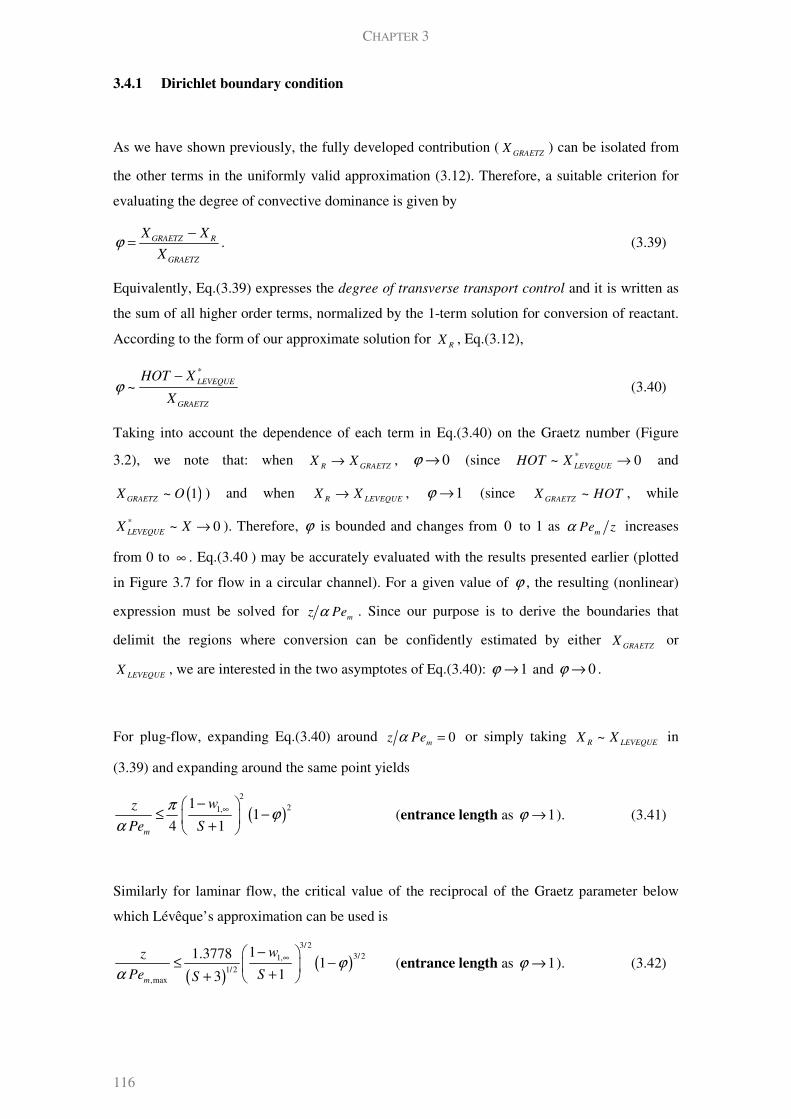
CHAPTER 3
116
3.4.1 Dirichlet boundary condition
As we have shown previously, the fully developed contribution (GRAETZ
X ) can be isolated from
the other terms in the uniformly valid approximation (3.12). Therefore, a suitable criterion for
evaluating the degree of convective dominance is given by
GRAETZ R
GRAETZ
X X
Xϕ
−= . (3.39)
Equivalently, Eq.(3.39) expresses the degree of transverse transport control and it is written as
the sum of all higher order terms, normalized by the 1-term solution for conversion of reactant.
According to the form of our approximate solution for R
X , Eq.(3.12),
*
~ LEVEQUE
GRAETZ
HOT X
Xϕ
− (3.40)
Taking into account the dependence of each term in Eq.(3.40) on the Graetz number (Figure
3.2), we note that: when R GRAETZ
X X→ , 0ϕ → (since *~ 0LEVEQUE
HOT X → and
( )~ 1GRAETZ
X O ) and when R LEVEQUE
X X→ , 1ϕ → (since ~GRAETZ
X HOT , while
* ~ 0LEVEQUE
X X → ). Therefore, ϕ is bounded and changes from 0 to 1 as m
Pe zα increases
from 0 to ∞ . Eq.(3.40 ) may be accurately evaluated with the results presented earlier (plotted
in Figure 3.7 for flow in a circular channel). For a given value of ϕ , the resulting (nonlinear)
expression must be solved for m
z Peα . Since our purpose is to derive the boundaries that
delimit the regions where conversion can be confidently estimated by either GRAETZ
X or
LEVEQUEX , we are interested in the two asymptotes of Eq.(3.40): 1ϕ → and 0ϕ → .
For plug-flow, expanding Eq.(3.40) around 0m
z Peα = or simply taking ~R LEVEQUE
X X in
(3.39) and expanding around the same point yields
( )
221,1
14 1
m
wz
Pe S
πϕ
α
∞−
≤ − +
(entrance length as 1ϕ → ). (3.41)
Similarly for laminar flow, the critical value of the reciprocal of the Graetz parameter below
which Lévêque’s approximation can be used is
( )( )
3/23/21,
1/2,max
11.37781
13m
wz
Pe SS
ϕα
∞−
≤ − ++
(entrance length as 1ϕ → ). (3.42)

BRIDGING THE GAP BETWEEN GRAETZ AND LÉVÊQUE’S THEORIES FOR MASS/HEAT TRANSFER
117
For the derivation of a criterion for the applicability of the one-term Graetz regime, we consider:
( )2
1, 1, ,maxexp 1m
w z Peλ α∞ ∞
− << , * 0LEVEQUE
X → but 1 2 ,maxmz Peα∆ >> ∆ . This set of
assumptions leads to
1,
2,max 2,
11ln
m
wz
Peα λ ϕ
∞
∞
− ≥
(fully developed regime as 0ϕ → ), (3.43)
valid for plug and laminar flows. Figure 3.7 shows the ϕ curve vs. the reciprocal of Graetz
number for a circular channel. Eqs.(3.42) and (3.43) are able to predict the result from (3.40)
with the uniform approximation outlined in section 3.2.2. For parallel plates, the agreement for
1ϕ → improves because there is no need to account for channel curvature. Plug-flow cases are
also better described since no linearization of the velocity profile near the wall is introduced.
Concerning the above criteria, we can make the following remarks:
(a) The variation in the value of m
z Peα in Figure 3.7 is more abrupt in the range where the
Graetz solution is adequate. This results in a bigger insensitivity to the criteria in this
regime, whereas in the definition of the applicability of Lévêque’s solution, the arbitrarily
fixed value of ϕ may induce large changes in the entrance length.
(b) The influence of the flow profile in the fully developed boundary is irrelevant. There are
numerical difficulties associated with the limit of 0ϕ → (near zero concentrations),
therefore Eq.(3.43) is particularly useful.
(c) The value of ϕ can be directly related with the relative error that occurs when estimating
conversion from the one-term Graetz solution:
GRAETZε ( )GRAETZ R R
X X X= − ( )1ϕ ϕ= − ~ ϕ . (3.44)
(d) The error that results from using Lévêque’s approximation (3.15) is given by LEV
ε
LEV R RX X X= − , which in the limit of 0
mz Peα → relates with ϕ according to:
( )( ) ( )
2 21,21, 1, 2
11 ~ 1
4 1LEV
ww
S
πε λ ϕ ϕ
∞
∞ ∞
−= − −
+
(plug flow) (3.45a)
( ) ( )( ) ( )
23/2 3/21, 1, 1,
1/2 3/2
11.3778 1 ~ 1
3 1LEV
w w
S S
λε ϕ ϕ
∞ ∞ ∞−
= − −
+ +
(laminar flow). (3.45b)
From Eq.(3.45), we can see that the error related with Lévêque’s solution is more sensitive
to the choice of ϕ , compared with (3.44). Also, the selection of the same value of ϕ for
plug and laminar flows results in a more conservative criterion for the former.
(e) Depending on the agreement required mainly with Lévêque’s original solution, the
transition region may extend by several orders of magnitude of m
z Peα .
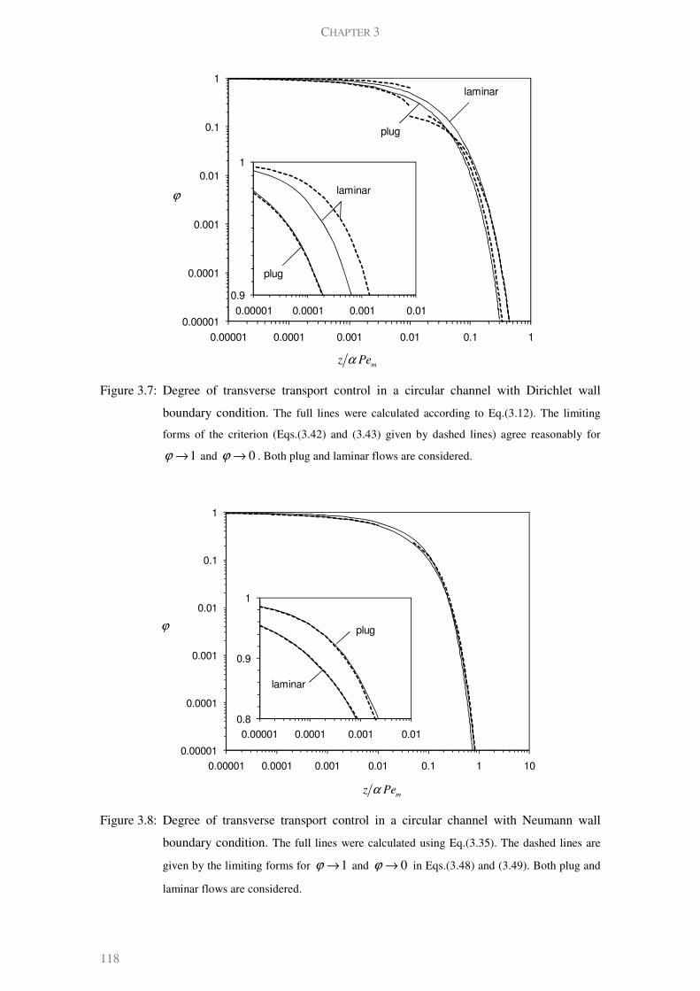
CHAPTER 3
118
Figure 3.7: Degree of transverse transport control in a circular channel with Dirichlet wall
boundary condition. The full lines were calculated according to Eq.(3.12). The limiting
forms of the criterion (Eqs.(3.42) and (3.43) given by dashed lines) agree reasonably for
1ϕ → and 0ϕ → . Both plug and laminar flows are considered.
Figure 3.8: Degree of transverse transport control in a circular channel with Neumann wall
boundary condition. The full lines were calculated using Eq.(3.35). The dashed lines are
given by the limiting forms for 1ϕ → and 0ϕ → in Eqs.(3.48) and (3.49). Both plug and
laminar flows are considered.
0.00001
0.0001
0.001
0.01
0.1
1
0.00001 0.0001 0.001 0.01 0.1 1
ϕ
mz Peα
0.9
1
0.00001 0.0001 0.001 0.01
laminar
plug
laminar
plug
0.00001
0.0001
0.001
0.01
0.1
1
0.00001 0.0001 0.001 0.01 0.1 1 10
0.8
0.9
1
0.00001 0.0001 0.001 0.01
mz Peα
ϕ plug
laminar
BRIDGING THE GAP BETWEEN GRAETZ AND LÉVÊQUE’S THEORIES FOR MASS/HEAT TRANSFER
119
These results define the length of the intermediate region between developing and fully
developed profile regimes. Operation and design in this range are of practical interest and
haven’t been sufficiently characterized. We have described analytically the transition from the
low conversion (small temperature change, 1ϕ → ) asymptote to the high conversion one
( 0ϕ → ). The same region marks the transition from low to high pressure drop regimes,
( )( )
3/22 1 1 , 1
~ ~ln , 0
mP u Pe
ϕ ϕρ α
ϕ ϕ
− − →
∆ − →
.
It is likely that an appropriate trade-off between achieving the required conversion/temperature
difference at the minimum pressure drop yields an optimum point in the gap between the two
well-described limits. The penalty in conversion so that pressure drop decreases by a certain
amount is related to the value of ϕ , as this measures the degree of agreement with the high
conversion (fully developed) asymptote. The simple and accurate results provided can be used
in optimization procedures, where many evaluations would be required. This may be
particularly useful on the simulation of multi-channel systems, at the integrated reactor level.
Another well-known trade-off occurs between conversion and mass transfer. The effect of an
entrance region is to increase the mass/heat transfer rate, compared to the fully developed
region, even though this is detrimental to the overall conversion. This increment can be
quantified in several ways (e.g. the incremental heat transfer number ( )N z given in Shah and
London (1978)). Therefore, ϕ also represents the increment in the transfer rate due to the
influence of the inlet and the effect being privileged (high mass transfer rates 1ϕ → , or high
conversions 0ϕ → ). Setting 0.01ϕ = corresponds to allowing the transfer rate at a given
position to be influenced by the inlet by 1%.
3.4.2 Neumann boundary condition
When the flux is uniform throughout the channel, we have separated developing and fully
developed contributions in the correlation for Sherwood (or Nusselt) number, Eq.(3.35). In this
case, a measure for profile development can be written as
1 1
1fd fd
fd
Sh Sh Sh Sh
Sh Shϕ
− −= = . (3.46)
If fd
Sh Sh>> (as it happens in the entrance length), then 1ϕ → . The fully developed region is
characterized by low values of ϕ (since 0ϕ → as fd
Sh Sh→ ). According to (3.35),
CHAPTER 3
120
LEV
fd LEV
HOTSh Sh
ϕ Θ= − − (3.47)
which can be completely determined with the information in section 3.3.2. This is plotted as a
function of m
z Peα for a circular channel in Figure 3.8. As previously, the limiting forms of
(3.47) are:
( ) ( )2 2
2
1 1
4m fd
Sz
Pe Sh
π ϕ
α
+ −≤ (entrance length as 1ϕ → for plug flow), (3.48a)
( )( )
33
3,max
10.55177 1
m fd
zS
Pe Sh
ϕ
α
−≤ +
(entrance length as 1ϕ → for laminar flow), (3.48b)
( )1,0 1
2,max 1,0
11ln
1fd
m
ShAz
Pe S
ϕ
α λ ϕ
− ≥
+ (fully developed regime as 0ϕ → ), (3.49)
valid for plug and laminar flows. The calculation of (3.47) from the uniformly valid solution
and the limiting forms (3.48) and (3.49) is shown in Figure 3.8 for a circular channel. In the
fully developed limit, the curves for plug and laminar flow overlap. The form of the curve in
Figure 3.8 is similar to the one in Dirichlet case (previous section) and therefore the same
comments are appropriate. Eq.(3.46) directly measures the deviation of the actual Sherwood
number from its fully developed value. On the other hand, the relative error associated with
Eqs.(3.31) is given by
1 1~ 1
1LEV LEV
LEV LEV
LEV
Sh Sh Sh Sh
Sh Shε
− −= = − Θ . (3.50)
Expanding Eq.(3.50) for 0m
z Peα → ,
( ) ( )
122,01
~1 1
q
LEV
m
z
q q Pe
λε
α
−
Γ − −
.
Substituting (3.48), LEV
ε can be related with ϕ :
( ) ( ) ( )2,0~ 1 1 ~ 1
LEV
fd
SSh
λε ϕ ϕ+ − − (plug flow) (3.51a)
( ) ( ) ( )
4/32 2 22,0
2~ 0.745201 1 1 ~ 1
LEV
fd
SSh
λε ϕ ϕ+ − − (laminar flow). (3.51b)
For the same value of ϕ , the criterion is more conservative for laminar flows.
Another interpretation of these results can be given in terms of the mass/thermal boundary layer
developing near the interface. The thickness of this region δ is related to the Graetz parameter
and it has been shown that it should be included e.g. in the criteria for delimitation of mass
BRIDGING THE GAP BETWEEN GRAETZ AND LÉVÊQUE’S THEORIES FOR MASS/HEAT TRANSFER
121
transfer – reaction regimes in a microreactor (Chapter 4). As in the case of the thermal/mass
entrance length, there is a lot of disparity in the definitions and values reported concerning δ .
In the case of uniform wall flux, we have obtained an explicit approximation for the
Sherwood/Nusselt number. From the theory of interphase transfer coefficients, we define the
thickness of the boundary layer ( a δ ) so that the mass/heat transfer coefficient is given by
( )~m
k D a δ . Thus, the Sherwood/Nusselt number can be written as ( ) ( ) ( )1Sh z S zδ= + .
The maximum boundary layer thickness is ( )1fd
S Shδ∞
= + . The normalized thickness so that
* 1δ = (boundary layer thickness equals the radius of the channel) for fully developed profile is
* fdSh
Sh
δδ
δ∞
= = .
Introducing Eq.(3.35) or(3.46):
* 1fd
fd LEV
LEV
Sh
Shδ ϕ= Θ + Θ = − .
In the case of a Dirichlet wall boundary condition, our criterion ϕ was formulated in terms of
conversion values, which makes the relationship with Sherwood number more complex. For
simplicity, and since we are looking for an estimate, the following expression is proposed:
( )( )1
* ~ 1q q
δ ϕ−
− ,
where 1 2q = for plug and 1 3q = for laminar flow. This allows both fully developed and
developing dependences of *δ on the Graetz parameter to be respected. The exact numerical
coefficients may differ a little from this estimate, but the correct order of magnitude is kept. We
note that according to Eqs.(3.45) at the inlet: * ~LEV
δ ε for plug flow and 1/3* ~LEV
δ ε for
laminar flow. On the other hand, according to Eq.(3.44) when the profile is near full
development: * ~ 1GRAETZ
δ ε− for plug flow and * ~ 1GRAETZ
δ ε− for laminar flow. The correct
estimation of this thickness is fundamental for the design of optimized microchannel systems,
where the complete or a fraction of the boundary layer is removed or disrupted by the periodic
placing of outlets or inlets (Yoon et al. 2006).
Expressing the dependence of Nusselt or Sherwood number on the Graetz parameter is often not
achieved by a single expression. Almost all correlations for Sherwood / Nusselt number are
given in branches with compartmented ranges of validity (usually, one for fully developed
conditions and other(s) for developing profile), and one can find many examples of this in Shah
and London’s book (Shah et al. 1978). Since each expression is constructed from asymptotic
limits, it is recognised that at the intersection of both asymptotes or in the limits of each interval,
the error in predicting Sherwood number is maximum. A curious consequence from (3.35) is an
estimate for the maximum error associated with this approach.

CHAPTER 3
122
At the intersection: fd LEV est
Sh Sh Sh= = (estimated Sherwood number). Then, the relative error
from this approach is given by
( )error 1 1est
fd LEV
Sh
Sh= − = − Θ + Θ .
This should be evaluated at the intersection point, which is given in Table 3.1 (criterion type B).
For laminar flow in a circular channel: error ~ 9% . In this case, the existence of an uniformly
valid solution to the interphase coefficient can reduce the error significantly.
From Figure 3.4, we can observe that fd
Θ and LEV
Θ intersect at ~ 0.01m
z Peα at a value of
~ 0.4 . At this point, ~ 0.5ϕ which corresponds to the intermediate level of profile
development. This validates the roles of fd
Θ , LEV
Θ and ϕ as being indicative of the degree of
profile development.
3.4.3 Comparison with previous criteria
In most of the chemical engineering literature, the ranges of validity of the entrance and fully
developed models have been obtained in a number of ways that we briefly detail below. Table
3.1 situates previous regime boundaries within our criterion by calculating the respective value
of ϕ . Data from the following five “calculation methods” are presented:
A. Analogy with the momentum boundary layer development length. For example, Kockmann
(2008) scale the entrance length for the concentration profile from the hydrodynamic length
yielding in our variables:
2
20.05 h
m
dz
Pe aα≤ .
In Table 3.1, we compare this with other criteria for laminar flow in a channel with Dirichlet
wall boundary condition.
B. Intersection of fully developed and Lévêque asymptotes in a m
Sh Pe zα− plot. In Chapter 4,
we calculated the value of the Graetz parameter where Lévêque’s correlation attained the fully
developed value. This is a usual procedure, which however ignores the intermediate region. In
this case, transition occurs around ~ 0.10ϕ .
C. Error comparison with numerical solution. Gervais and Jensen (2006) determined the
intersection of absolute error curves from 1D models with developing and fully developed
correlations for Sh . Their result for laminar flow between parallel plates with symmetric
boundary conditions is in Table 3.1.

BRIDGING THE GAP BETWEEN GRAETZ AND LÉVÊQUE’S THEORIES FOR MASS/HEAT TRANSFER
123
D. Agreement with fd
Sh by an arbitrarily defined margin of error. The reference book from
Shah and London (1978) presents the distance required to achieve a local Nusselt number equal
to 1.05 of the fully developed temperature profile value. Polyanin et al. (2002) also calculate the
length of the thermal initial region so that 1.01fd
Nu Nu= . Table 3.1 contains these results for
laminar flow. It can be seen directly in the case of Neumann boundary condition, that our
criteria confirms these results.
E. Agreement between analytical solutions. Shah and London (1978) give the range of
mz Peα , where the Nusselt number calculated from the 120-term Graetz series equals the one
from the 7-term Lévêque series up to 5 or more digits. In addition, Alonso et al. (2010)
identified the transition region in laminar flow inside a circular channel with wall concentration
annulment ( 0.05 0.2m
z Peα≤ ≤ ). This is also included in Table 3.1 for comparison.
From these few examples in the literature, we can make the following comments:
(a) As expected, most available information refers to the value of the Graetz parameter below
which the fully developed profile is adequate. Much less information concerning the
validity of Lévêque’s solution is provided. The finite transition region between both
regimes is also frequently ignored.
(b) There is a large variation in the boundaries that are provided, sometimes by one-order of
magnitude. This is reflected in terms of ϕ values, and consequently on the relative error
incurred by the use of approximations (see e.g. Eqs.(3.44) and (3.45)).
(c) When provided, the boundary for the developing profile given by Lévêque’s solution is
usually overestimated (values of ϕ not high enough).
Despite this and the fact that the concept of thermal/mass profile development length is well
established, it is a common practice to propose criteria for the negligibility of entrance effects
with no relationship to the arbitrary basis on which they were formulated and without the
information that the analytical solution provides. Instead, an order of magnitude for the Graetz
parameter is often preferred. Recently, Morini (2006) proposed that inlet effects on the average
Nusselt number can be neglected if ( )2 10h
Gz u d D L= < . From Figure 3.7, we can see that
this corresponds to ( )1
0.4m
Peα−
> and to a very conservative (low) value of ϕ . Moreover,
order of magnitude results ignore the correct numerical coefficients, which distinguish different
shapes and flow conditions.

CHAPTER 3
124
Table 3.1:Comparison of the ranges of validity given in the literature with our criteria.
Shape Flow
profile
Boundary
condition
Criterion
type m
z
Peα ϕ Ref.
Cir
cula
r
Lam
inar
Dirichlet
A 0.2 0.002 Kockmann (2008)
Alonso et al. (2010)
B 0.1021 0.03 Chapter 4
D 0.22 0.001 Polyanin et al. (2002)
0.1339 0.01 Shah and London (1978)
E 58 10−> × 0.974
0.02< 0.315
0.05> 0.108 Alonso et al. (2010)
Neumann
B 0.1063 0.09 Chapter 4
D 0.28 0.01 Polyanin et al. (2002)
0.1722 0.04 Shah and London (1978)
E 48 10−> ×
0.80
0.02<
0.40
Plu
g
Dirichlet B 0.0381 0.10 Chapter 4
Neumann B 0.0491 0.27
Pla
tes Lam
inar
Dirichlet
A 0.8 9~10− Kockmann (2008)
B 0.07 0.07 Chapter 4
C 0.24 0.001 Gervais and Jensen (2006)
D 0.1276 0.014 Shah and London (1978)
E 0.008> 0.58
0.016< 0.43
Neumann
B 0.0948 0.14 Chapter 4
D 0.1847 0.045 Shah and London (1978)
E 0.008> 0.57
0.08< 0.17
Plu
g
Dirichlet B 0.0523 0.1 Chapter 4
Neumann B 0.0873 0.26

BRIDGING THE GAP BETWEEN GRAETZ AND LÉVÊQUE’S THEORIES FOR MASS/HEAT TRANSFER
125
We note that in principle the analysis can be extended to channels with different cross-sectional
shapes. From WKB theory for large eigenvalues, curvature is negligible at the region near the
interface, and therefore the dependence of eigenvalues and weights on n should be
approximately the same. The correct values for 1λ and 1w can be calculated numerically or
taken from the literature (Shah et al. 1978; Kays et al. 1980) for many geometries. Lévêque’s
solution can also be extended using a normalization based on the friction factor (Shah et al.
1978). At the convective dominated regime, shape effects are negligible at the boundary layer
and it is only required to include the correct linearization for the laminar velocity profile. The
same applies to other Graetz problems that have appeared in the literature (Weigand et al. 2007;
Haji-Sheikh et al. 2009; Aydin et al. 2010; Ray et al. 2010; Vera et al. 2011) and received the
same analytical treatment, as long as an asymptotic description of coefficients is available.
3.5 FINITE LINEAR WALL KINETICS
We now extend the approach outlined in sections 3.2 and 3.3 to the case of Robin boundary
condition, i.e. when a finite reaction rate occurs at the wall (or for finite wall thermal
resistance). In this case, Eq.(2.4) is valid at the wall
( )1
1,r
cDa c z
r=
∂= −
∂, (2.4)
where Da is the Damköhler number for a first-order reaction (surf
k a Dη= ). According to
Graetz’s series solution, the mixing-cup concentration profile is given by Eq.(3.2), where the
eigenvalue n
λ and coefficient n
w are dependent only on Da for each channel geometry and
flow profile. In Chapter 2, we have presented empirical correlations that describe the variation
of these quantities as a function of Da , between two plateaus in the limits of 0Da → and
Da → ∞ , where Neumann and Dirichlet-type boundary conditions are recovered, respectively.
In the context of heat transfer, a similar boundary condition applies when the wall resistance
(noted by w
R in Shah and London (1978)) is finite. We intend to obtain a solution which is
uniformly valid on Da (or w
R ) and on Graetz’s parameter (m
Pe zα ).
3.5.1 Assumptions on the dependence of eigenvalues and coefficients
In this case, it is also fundamental to assume that the spacing between consecutive eigenvalues
(i.e. between n
λ and 1nλ
+) is constant. Previously (in the Neumann and Dirichlet limits of
CHAPTER 3
126
Eq.(2.4)), the asymptotic behavior of eigenfunctions appearing at the wall boundary condition
predict nearly uniform spacing as n increases (as the eigenvalues become larger). However, for
the first eigenvalues this is also reasonable and in those cases:
( )1 1n
nλ λ λ= + − ∆ ( 1,2...n = ) (3.52)
4
πλ
∆ =
(plug-flow)
(laminar flow) (as n → ∞ ). (3.10)
For finite reaction rate conditions (finite Da ), the spacing between the first couple of
eigenvalues ( ),n
n Daλ∆ may depend not only on n , but also on Da (it has a minimum around
~ 1Da , more pronounced for 1n = ). When 0Da → , Da → ∞ or n is large, Eqs.(3.52) and
(3.10) are satisfactorily fulfilled. Since higher eigenvalues are associated with terms of
decreasing importance (namely, exponential terms with negative arguments), we will consider
that these relationships are also adequate for finite Da . This assumption will reduce the
complexity of the final solution as shown below.
Concerning the dependence of coefficients on eigenvalues, the exact values of n
w (when Da
finite) are given for plug flow by
( )
2
2 2 2
2
1n
n n
Daw
Da Da S
σ
λ λ σ=
+ + − ( 1,2...n = ). (3.53)
Numerically calculated values of 1λ should be used in Eq.(3.53) for accurate calculations when
1n = . When the flow is fully developed and for high eigenvalues, WKB theory gives the
following results,
7/3, ,2.02557
n nw σ λ
−
∞ ∞= ( Da → ∞ , 1
nλ >> ) (3.54a)
2 11/3,0 ,02.4010
n nw Daσ λ
−= ( 0Da → , 1
nλ >> ). (3.54b)
When , the first eigenvalue also tends to zero according to
( )2
2 31
,0
1
fd
SDa Da O Da
Sh
λ
σ
+= − + (3.55)
and the estimate from (3.54b) is not adequate. Instead, we use the asymptotic expansion for
small eigenvalues,
( )
2
2 31
,0
11
fd
Sw Da O Da
Sh
+= − +
(3.56)
where ,0fdSh is given by Eqs.(3.27). In this limit, (3.53) writes as (plug-flow):
2 42n n
w Daσ λ= ( 1n > and ( )~ 1n
Oλ ).
0Da →

BRIDGING THE GAP BETWEEN GRAETZ AND LÉVÊQUE’S THEORIES FOR MASS/HEAT TRANSFER
127
3.5.1.a Simplified dependence of weights
Taking into account the behavior for large eigenvalues, we assume that higher coefficients can
be calculated from the first one according to
1 1n nw w
β βλ λ= ( 2,3...n = ), (3.57)
where 0β β β∞
≤ ≤ . According to Eqs.(3.53) and (3.54), β changes from its value in the
Dirichlet limit ( β∞
) to the one in the small Da asymptote ( 0β ). For plug-flow,
( )( )
( )
2 21
0
1
ln, 0 2 4
ln
n
n
n Daλ λ
β βλ λ
= → = + = (3.58a)
( )( )
( )1
ln 1, 2 2
lnn
n Daβ βλ λ
∞= → ∞ = + = . (3.58b)
For laminar flow,
( )
( )
21,0 ,0 ,0
01,0,0 1,0
ln ln ln~ ~ 4
lnln ln
n n
n
w w w Da
Daβ
λλ λ= = (3.59a)
( )
( )
1, ,
, 1,
ln 7
3ln
n
n
w wβ
λ λ
∞ ∞
∞
∞ ∞
= = . (3.59b)
The form of ( )Daβ will be provided in different cases as detailed in the next section.
3.5.2 Contributions to the mixing-cup concentration profile
The assumptions outlined in the previous section allow us to write Eq.(3.2) as
( )0
limN
Nn
c f n→∞
=
= ∑ , where:
( )( )
( )2
11 1
,max1
expm
n zwf n
Pen
β
β
λ λλ
αλ λ
− + ∆ = + ∆
( 0,1,2...n = ). (3.60)
An asymptotic approximation to the summation of terms given by (3.60) can again be obtained
by the Euler-Maclaurin sum formula (Bender et al. 1978). After some simplifications and
removing the negligible terms, the following expression is obtained:
R GRAETZ fd LEVX X LEV= Θ + Θ (3.61)
Each one of the terms in Eq.(3.61) can be calculated as follows. The first term in Graetz series
corresponds to the fully developed solution and is given by
21
1,max
1 expGRAETZ
m
zX w
Pe
λ
α
−= −
. (3.62)

CHAPTER 3
128
The approximation of the conversion profile by this solution was discussed in Chapter 2 for
finite reaction rates. The fd
Θ factor measures the importance of (3.62) compared with the other
terms in (3.2) that are not retained (far from the inlet), and includes the second term in Graetz’s
series (this is related to the HOT term in section 3.2.2),
( )
( )
22 2 ,max
21 1 ,max
exp1
1 exp
m
fd
m
w z Pe
w z Pe
λ α
λ α
∆ −Θ = −
− − (3.63)
1 2,maxm
z
Peα∆ = ∆ + ∆ . (3.64)
From section 3.5.1, 2w and 2λ can be easily estimated, if necessary resorting to the definition
of β , which is calculated as described in sections 3.5.2.a and 3.5.2.b. The coefficients in (3.64)
only require the knowledge of the first eigenvalue according to
11
2
1 w
w
−∆ = (3.65a)
2 26
λλ
∆∆ = . (3.65b)
Rigorously another result is obtained for 1∆ , but is has been shown that replacing it by
Eq.(3.65 a) (so as to fulfill the inlet boundary condition) is reasonable (section 3.2.2). The
second term in (3.61) is related with the contribution of Lévêque’s solution, and includes two
factors: the first one ( LEV ) is a correction/limit of the entry length profile; the second one is a
corrective incomplete gamma function, which we have identified as a normalized measure of
the importance of LEV (section 3.2.2), as discussed below. Both are given by:
( )
( )1 /2
1 1
,max
3
1 2m
w zLEV
Pe
ββ
λ β
λ β α
−
− = Γ ∆ −
(3.66)
( )
22
,max
1 3,
3 2 2 2LEV
m
z
Pe
λβ
β α
−Θ = Γ Γ −
. (3.67)
In the entrance region of the channel (for small m
z Peα ), the conversion of reactant according
to Eqs.(3.61) to (3.67), writes as
( )
( )1 /2
1 1
,max
3
1 2R
m
w zX
Pe
ββ
λ β
λ β α
−
− = Γ + ∆ −
( )( )( )
232 2 2 2
1 1 2 2 1 2,max
2
1 3m m
w z zw w O
Pe Pe
λλ λ
λ β β α α
+ + ∆ − ∆ + +
∆ − − . (3.68)
BRIDGING THE GAP BETWEEN GRAETZ AND LÉVÊQUE’S THEORIES FOR MASS/HEAT TRANSFER
129
The first term in (3.68) is LEV , while at ( )mO z Peα contributions from
GRAETZ fdX Θ (the two
first terms inside square brackets) and LEV
LEV Θ (the third term inside brackets) appear, since
( )
( )
( )
( )( )
3 22
3 2 12
,max
2 31
3 2 2LEV m
m
zO z Pe
Pe
β
ββ λα
β α
−
− + − Θ = − + Γ −
(3.69a)
( )
222 21 1 2 2
21 ,max1fd m
m
w w zO z Pe
w Pe
λλ α
α
− ∆ Θ = + + − . (3.69b)
Note that the description of the entry length is greatly influenced by the range of values taken by
β . This can be seen namely in the definition of the dominant term in (3.68) and the magnitude
(and sign) of LEV
Θ in (3.69a).
In conditions far from the developing length (i.e. large m
z Peα ), the weighting functions of the
developing and fully developed solutions change their behavior, confirming their role as
measures for the two contributions to the conversion profile. Namely, 1fd
Θ → and 0LEV
Θ →
according to:
( )
( )1 22 2
,max 2 222 ,max ,max
1 1~ 1 exp
3 2 2 2m
LEV
m m
Pe z z
z Pe Pe
β
α λ λβ
β λ α α
−
−−Θ − Γ −
(3.70a)
22
2,max
~ 1 expfd
m
zw
Pe
λ
α
−Θ − ∆
. (3.70b)
The values taken by β have little influence in this case (the calculation of 2w is only slightly
changed). Thus, the profile is dominated by the fully developed solution,
22,max2 2
2 2,max 2
1exp
1 2m m
R GRAETZ
m
Pe PezX X w O
Pe z z
α αλ λ
α λ β λ
− = − ∆ − − + ∆ −
. (3.71)
Since there is a significant change in the analysis, depending on the value taken by β , two sets
of values are considered separately: 03 β β< ≤ (which includes the kinetic controlled regime)
and 3β β∞
≤ < (representing in the limit, the mass transfer controlled regime). In each region, a
calculation procedure for conversion and for the function ( )Daβ is provided. The transition
limit (when 3β = ), occurs at a value of Damköhler number T
Da , which we calculate below as
being around 1.
CHAPTER 3
130
3.5.2.a Values of 03 β β< ≤ ( ~ 1T
Da Da< )
When 3β > , the term in Eq.(3.68) of ( )mO z Peα becomes dominant, while LEV is of
( )( )1 /2
mO z Pe
β
α−
, representing a correction. In the kinetically controlled limit ( 0Da → ), the
inlet regime described by (3.68) is dominated at ( )mO z Peα by ( )~
GRAETZ fdX O DaΘ ,
followed by terms related with fd
Θ and LEV
LEV Θ , both of ( )2
O Da . The relative importance
of the two latter terms (inside brackets in (3.68)) is given by ( )( )1 1 3 2β β∆ − − . Noting that
( )1 1 21 w w∆ = − takes its highest value (which may be 1>> ) when Da is low ( 4β → ), it is
possible the contribution from LEV
LEV Θ to be negligible compared with GRAETZ fd
X Θ . Also,
note that as 3β → the importance of the contribution from LEV
LEV Θ at the inlet may increase
significantly, leading to an inconvenient singularity. To place this contribution in the correct
relative magnitude compared to other terms, we will take
0 4β β= = for T
Da Da< , (3.72)
where the transition value T
Da is around 1, although its precise value will be determined in
section 3.5.2.b. According to (3.72), the approximation to conversion with an ( )2
O Da term in
the kinetic limit is given by
2 2
2,max ,0 ,max
1 5~ ...
6R
m fd m
Da z S Da zX
Pe Sh Pe
σ σ
α λ α
+− + + ∆
(for 1m
z Peα << ) (3.73a)
22
2
,max ,max ,0 ,max ,0
1 1 1~ ...
2R
m m fd m fd
Da z z S z SX Da
Pe Pe Sh Pe Sh
σ σ
α α α
+ + − + − +
(for 1m
z Peα >> ) (3.73b)
While the ( )2
O Da term in Eq.(3.73a) has a contribution from the developing parcel
LEVLEV Θ , (3.73b) only reflects the fully developed profile influence. Examining the solutions
in Levêque’s regime (Carslaw et al. 1959; Ghez 1978) presented in Chapter 2 for 1Da << ,
( )
3/2234
3LEV
m m
Da z Da zX O Da
Pe Pe
σ σ
α απ
= − +
(plug flow) (3.74a)
( )
4/3
5/32 3
,max ,max
0.9144LEV m
m m
Da z zX Da O Da z Pe
Pe Pe
σσ α
α α
= − +
(laminar flow) (3.74b)

BRIDGING THE GAP BETWEEN GRAETZ AND LÉVÊQUE’S THEORIES FOR MASS/HEAT TRANSFER
131
we observe that the ( )2
O Da corrections to the leading-order behavior are smaller than
( )mO z Peα . Comparing with Eq.(3.73a), only the leading-order behavior (equal in
LEVX and
GRAETZX for 0
mz Peα → ) is reproduced. Therefore, the contribution of LEV is not to
represent conversion in Lévêque’s limit, but only a ( )2
O Da correction to that solution in an
higher order contribution of ( )mO z Peα .
3.5.2.b Values of 3β β∞
≤ < ( ~ 1T
Da Da> )
When 3β < , the entry length solution (3.68) is given by LEV , followed by a correction of
( )mO z Peα . In contrast with the kinetic limit (where the leading-order term from
LEVX and
GRAETZX is the same), the contributions from fully developed and developing regimes in mass
transfer control are completely separable. Actually, LEV
LEV X= when Dirichlet boundary
condition is applicable (section 3.2.2). Therefore, in this range of β we should take LEV as
approximately LEV
X (had this been done for 3β > and the leading order term would have come
up repeated). An approximate solution to Lévêque’s problem has been given in Chapter 2:
( )1
1 2m
LEV
m
S Da z PeX
Da z Pe
α
π α
+=
+ (plug flow) (2.33)
( )
,max
1/3
,max1 0.9828
m
LEV
m
Da z PeX
Da z Pe
σ α
α
=
+
(laminar flow). (2.35)
Eq.(3.61) becomes
R GRAETZ fd LEV LEVX X X= Θ + Θ (3.75)
where all the terms were defined previously in Eqs.(3.62), (3.63) and (3.67). To complete the
calculation procedure, namely to calculate 2w from (3.57) and LEV
Θ from (3.67), an estimated
relationship for β has to be provided. It is also desirable to know how β varies with Da . In
general, ( ),n Daβ β= and according to (3.57):
( )( )
( )
1
1
ln,
lnn
n
w wn Daβ
λ λ= . (3.76)

CHAPTER 3
132
(a) Plug flow
(b) Laminar flow
Figure 3.9: β as a function of the Damköhler number Da . Planar and circular channel with (a)
plug flow or (b) laminar flow. Full lines are calculated from Eqs.(3.77) and (3.79) with no
numerical evaluation involved (approximation for 1λ was used). If approximations for
large Da are sought, Eq.(3.78) can be used, shown by the dashed lines in (a). For
TDa Da< , the dashed variation of β should be replaced by the branch given by 4β = .
2
2.2
2.4
2.6
2.8
3
3.2
3.4
3.6
3.8
4
0.0001 0.001 0.01 0.1 1 10 100 1000
Da
β
circular
plates TDa
2
2.2
2.4
2.6
2.8
3
3.2
3.4
3.6
3.8
4
0.0001 0.001 0.01 0.1 1 10 100 1000
Da
β
7 3β∞
=
TDa

BRIDGING THE GAP BETWEEN GRAETZ AND LÉVÊQUE’S THEORIES FOR MASS/HEAT TRANSFER
133
In order to proceed, it is necessary to assume that ( ) ( ),n Da Daβ β= , i.e. β is independent of
n . Moreover, since the purpose of defining β is to correctly estimate coefficients that get
significantly smaller as n increases (according to (3.60)), then ( ) ( ), ~ 2,n Da n Daβ β = .
Higher weights tend to zero fast, so the approximation benefits from accurately estimating the
second weight. For plug-flow, according to Eq.(3.53):
( )
( )
( )
2 22
2 212 1
112 ln
1ln
Da Da S
Da Da S
λ σβ
λ σλ λ
+ + −= + + + −
(plug flow). (3.77)
Note that in Eq.(3.77): 2 1λ λ λ= + ∆ and 1λ can be estimated as described in section 3.5.1
(numerically or approximately). Figure 3.9a shows the plot according to (3.77) as well as the
limiting form for large Da :
( )( )
1, 2, 32
2, 1,lnO Da
Da
λ λ λβ β
λ λ
∞ ∞ −
∞
∞ ∞
+ ∆= + + (plug-flow, Da → ∞ ). (3.78)
with 2, 1,λ λ λ∞ ∞
= + ∆ (plug). Eq.(3.78) is useful for 20Da > . Alternatively, the coefficient β
can be fitted obviously in a number of ways. For simplicity and with minimum numerical
evaluation, the following empirical correlation for laminar flow is proposed:
( )0
1
DaDa
Da
β ββ
∞+
=+
(laminar flow). (3.79)
Eq.(3.79) represents numerical results of (3.76) with 2n = , very accurately for T
Da Da> .
Also, in laminar flow insensitivity to the channel’s geometry is observed. Note that for high
Da , Eq.(3.79) writes as ( ) ( )0Da Daβ β β β∞ ∞
= + − , which is of the same form of the
expansion of (3.76) for Da → ∞ . Eq.(3.79) is plotted in Figure 3.9b for laminar flow. It also
fulfills our requirements of simple evaluation, without introducing additional parameters and
avoiding fitting. From (3.77) and (3.79) with ( ) 3T
Daβ = , the value of Damköhler number
which marks the transition is 1.5T
Da = for laminar flow, 1.6T
Da ≃ for plug flow between
parallel plates and 2.9T
Da ≃ for plug flow inside a circular channel.
The variation of fd
Θ and LEV
Θ with Da and m
z Peα is plotted in Figure 3.10 and Figure
3.11, respectively. The weighting function of the fully developed profile fd
Θ changes
significantly at low kinetic rates, with increasing importance as 0Da → , where 1fd
Θ → closer
to the inlet. The behavior of LEV
Θ also changes significantly, with T
Da Da= being the turning
point between negative and positive values. When 3β > , LEV
−Θ decreases as m
z Peα and
Da increases. When 3β < , LEV
Θ increases with Da and it approaches unity at much higher
mz Peα for high Da , than it does for intermediate values.
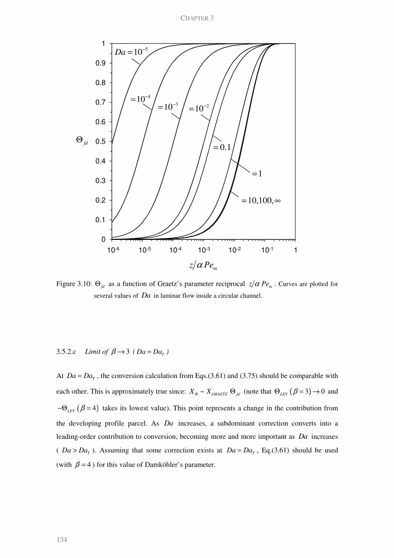
CHAPTER 3
134
Figure 3.10: fd
Θ as a function of Graetz’s parameter reciprocal m
z Peα . Curves are plotted for
several values of Da in laminar flow inside a circular channel.
3.5.2.c Limit of 3β → (T
Da Da= )
At
TDa Da= , the conversion calculation from Eqs.(3.61) and (3.75) should be comparable with
each other. This is approximately true since: ~R GRAETZ fd
X X Θ (note that ( )3 0LEV
βΘ = → and
( )4LEV
β−Θ = takes its lowest value). This point represents a change in the contribution from
the developing profile parcel. As Da increases, a subdominant correction converts into a
leading-order contribution to conversion, becoming more and more important as Da increases
( T
Da Da> ). Assuming that some correction exists at T
Da Da= , Eq.(3.61) should be used
(with 4β = ) for this value of Damköhler’s parameter.
0
0.1
0.2
0.3
0.4
0.5
0.6
0.7
0.8
0.9
1
1.E-06 1.E-05 1.E-04 1.E-03 1.E-02 1.E-01 1.E+00
fdΘ
mz Peα
10-6 10-5 10-4 10-3 10-2 10-1 1
510Da−
=
410−=
310−= 210−
=
0.1=
1=
10,100,= ∞

BRIDGING THE GAP BETWEEN GRAETZ AND LÉVÊQUE’S THEORIES FOR MASS/HEAT TRANSFER
135
(a)
TDa Da<
(b)
TDa Da>
Figure 3.11: LEV
Θ as a function of Damköhler and Graetz’s parameters. (a) For T
Da Da< ,
where 0 4β β= = . (b) For T
Da Da> , where ( )Daβ is given by Eqs.(3.77) and (3.79).
0.001
0.01
0.1
1
10
100
1000
1.E-06 1.E-05 1.E-04 1.E-03 1.E-02 1.E-01 1.E+0010-6 10-5 10-4 10-3 10-2 10-1 1
mz Peα
LEV−Θ 0.01Da =
0.1Da =
1Da =
1.5T
Da =
0
0.1
0.2
0.3
0.4
0.5
0.6
0.7
0.8
0.9
1
1.E-06 1.E-05 1.E-04 1.E-03 1.E-02 1.E-01 1.E+0010-6 10-5 10-4 10-3 10-2 10-1 1
mz Peα
LEVΘ
2Da =
100Da =
10Da =
1.5T
Da =

CHAPTER 3
136
3.5.3 Calculation procedure for the conversion profile
According to this analysis, the estimation of conversion for given values of Da and m
z Peα
can be summarized into the following steps:
1. For a given Da , calculate 1w and 1λ numerically or approximately according to the results
in section 3.5.1.
2. Choose a suitable value for β , according with the value of T
Da :
( )
0 4
Da
ββ
β
==
T
T
Da Da
Da Da
≤
>
where ( )Daβ is given by Eq.(3.77) for plug flow and by Eq.(3.79) for laminar flow.
3. The second weight 2w and eigenvalue 2λ can be simply calculated from step 1, using
Eqs.(3.52) and (3.57) with the appropriate value of β .
4. For each value of Da and m
z Peα , calculate fd
Θ and LEV
Θ . These functions are plotted
in Figure 3.10 and in Figure 3.11 for laminar flow inside a circular channel.
5. Calculate conversion according to Eq.(3.61) for T
Da Da≤ , and with (3.75) for T
Da Da> ,
evaluating GRAETZ
X and LEV or LEV
X with Eqs.(3.62) and (3.66) or (2.33, 2.35),
respectively.
For laminar flow inside a circular channel, where a first-order heterogeneous reaction occurs,
Figure 3.12 compares the uniform solution calculated as described above, with Graetz’s series
with 1 and 12 terms for several values of Da . The terms in Graetz’s series used for comparison
were calculated numerically when available (Özisik et al. 1982) or from asymptotic
relationships (section 3.5.1). The LEV
LEVΘ or LEV LEV
XΘ terms are also shown. It is possible
to observe the increase in the importance of this term as Da increases. The consistent evolution
of its magnitude legitimates our choice for the calculation at T
Da and the substitution of LEV
by LEV
X when T
Da Da> . Note that this replacement allows the inlet region to be described
correctly for T
Da Da> (where LEV
Θ is not vanishingly small). The convergence of Graetz’s
series also gets worse as Da increases. In particular, the adequacy of the first term in the series
becomes extremely limited as the reaction rate increases. The agreement of our solution
increases as more terms in Graetz’s series are considered, meaning that the approximate result is
at least comparable with the exact solution with a reasonable number of terms which depend on
numerically calculated quantities. Similar behavior for other geometries and flow profiles is
observed.

BRIDGING THE GAP BETWEEN GRAETZ AND LÉVÊQUE’S THEORIES FOR MASS/HEAT TRANSFER
137
(a)
(b)
(c)
(d)
Figure 3.12: Conversion in laminar flow inside a circular channel with first-order wall reaction
as a function of Graetz’s parameter m
z Peα for several values of Damköhler’s
number Da . Graetz series solution (3.2) with 1, 5 and 12 terms is shown.

CHAPTER 3
138
(e)
(f)
Figure 3.12: Conversion in laminar flow inside a circular channel with first-order wall reaction
as a function of Graetz’s parameter m
z Peα for several values of Damköhler’s
number Da . Graetz series solution (3.2) with 1, 5 and 12 terms is shown.
3.5.4 Developing length of the concentration profile
By explicitly identifying the contribution from the fully developed profile (the first term in
Graetz series), it is possible to estimate the length of profile development. We are particularly
interested in understanding the applicability of the fully developed asymptote as 0Da → . This
is motivated by the fact that the results from the Neumann boundary condition in section 3.3 do
not reflect several remarks that have been made in this work and in the literature. Namely,
(a) the error in estimating conversion with one term in Graetz series when m
Pe zα
increases is more significant for high values of Da (as seen in Chapter 2);
(b) at leading-order as 0Da → , fully developed and Lévêque solutions coincide near the
inlet (see section 3.5.2.a);
(c) fd
Θ (which measures the importance of the fully developed limit) reaches values close to
1 at lower m
z Peα when 0Da → (Figure 3.10); and
(d) Gervais and Jensen (2006) concluded that the importance of the fully developed
description increases when 0Da → , comparing simplified models with the numerical
solution.

BRIDGING THE GAP BETWEEN GRAETZ AND LÉVÊQUE’S THEORIES FOR MASS/HEAT TRANSFER
139
Moreover, it is also recognized (Gervais et al. 2006) that the critical value of Graetz’s parameter
at which Lévêque’s model is no longer satisfactory cannot be determined from a straightforward
approach when Da is finite, and that the required numerical evaluation is tedious. Nevertheless,
they show that terms in Graetz series, other than the first, decay much faster for lower Da , and
this results in reduction of the absolute error of the fully developed asymptote by one order-of-
magnitude at the inlet.
We can make use of the degree of transverse control introduced previously and given by
Eq.(3.39), which is related to the relative error of the one-term Graetz solution by Eq.(3.44). We
will focus on the derivation of the profile development length (i.e. low values of ϕ or GRAETZ
ε ).
In the kinetic limit ( 0Da → ), low error of the Graetz asymptote is obtained near the inlet
( 0m
z Peα → ). In these conditions, we assume LEV GRAETZ fd
LEV XΘ << Θ , and therefore:
2
,max1
,0
1~ 1 ~ m
GRAETZ fd
fd
Pe SDa
z Sh
αε
σ
− +
Θ −
(3.80)
For ( )~ 1m
z Pe Oα , 0GRAETZ
ε → faster, so Eq.(3.80) can be defined as a boundary. At the
diffusional limit ( Da → ∞ ), when the fully developed solution is appropriate: 0LEV
Θ → and
fdΘ is reasonably insensitive to kinetics as shown in Figure 3.10. Therefore, the Dirichlet limit
detailed in section 3.4.1 is recovered again and the length of development is nearly insensitive
to the fast kinetics:
( )2 22, 2,
2, 1,,max ,max
~ 1 ~ exp ~ 1 expGRAETZ fd
m m
z zw w
Pe Pe
λ λε
α α
∞ ∞
∞ ∞ ∞
− −− Θ ∆ −
. (3.81)
Other limits are more complex. We propose a formula that correlates both behaviours from
(3.80) and (3.81) as
( )
12,0,max 1,2
2,2
1ln
1
fdm GRAETZ
GRAETZ
ShPe w
z Da S
α εσ λ
ε
−
∞
∞
− = +
+ (3.82)
which is valid for small GRAETZ
ε and can be written explicitly for Da . For circular channel with
laminar flow, the ( )mDa z Peα curves for several values of
GRAETZε are plotted in Figure 3.13.
Qualitatively, this represents the expected trend even though quantitatively some adjustments
may be required.
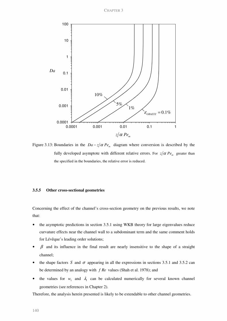
CHAPTER 3
140
Figure 3.13: Boundaries in the m
Da z Peα− diagram where conversion is described by the
fully developed asymptote with different relative errors. For m
z Peα greater than
the specified in the boundaries, the relative error is reduced.
3.5.5 Other cross-sectional geometries
Concerning the effect of the channel’s cross-section geometry on the previous results, we note
that:
• the asymptotic predictions in section 3.5.1 using WKB theory for large eigenvalues reduce
curvature effects near the channel wall to a subdominant term and the same comment holds
for Lévêque’s leading order solutions;
• β and its influence in the final result are nearly insensitive to the shape of a straight
channel;
• the shape factors S and σ appearing in all the expressions in sections 3.5.1 and 3.5.2 can
be determined by an analogy with f Re values (Shah et al. 1978); and
• the values for 1w and 1λ can be calculated numerically for several known channel
geometries (see references in Chapter 2).
Therefore, the analysis herein presented is likely to be extendable to other channel geometries.
0.0001
0.001
0.01
0.1
1
10
100
0.0001 0.001 0.01 0.1 1
Da
mz Peα
0.1%GRAETZ
ε =
1%5%
10%

BRIDGING THE GAP BETWEEN GRAETZ AND LÉVÊQUE’S THEORIES FOR MASS/HEAT TRANSFER
141
3.6 CONCLUSIONS
We have derived an approximate analytical solution to Graetz’s problem in terms of a
combination of the fully developed and developing (Lévêque’s) limits. Our solutions for the
mixing-cup concentration/temperature profile or for Sherwood number, as a function of the
axial distance, have the following features: (a) accurate results are obtained over the full range
of the Graetz number (m
Pe zα ); (b) relative error does not increase sharply in any specific
range; (c) both limiting regimes are respected and the gap between them is well described; and
(d) the form of the analytical solution is much simpler than any of the existing (involving a large
number of terms with numerically determined coefficients) and minimum numerical evaluation
is required. Mixing-cup concentrations are described with a maximum of 0.1% relative error
(except for laminar flow between parallel plates, where the error is higher but still tolerable).
When the wall boundary condition is of Neumann type, a solution for the Sherwood number
based on adding the entrance length and fully developed terms is given. Each term has an
associated weighting function, for which analytical expressions are provided. We have also
extended the analysis to the case where a finite reaction rate at the wall occurred.
Finally, we define criteria for transition between regimes which reflect the relative errors
obtained by using the fully developed or Lévêque solutions. Explicit expressions for the length
of the profile development zone are provided as a function of a desired degree of agreement
with the fully developed solution, channel geometry, flow profile and boundary condition type.
Previous disperse results in the literature are framed in a common analysis. Ranges of validity
for the developing profile asymptote are given, as well as estimates for the length of the
transition region. The approach presented can be extended to the analysis of Graetz or other
chemical engineering problems.
NOTATION
a radius of the circular channel or half-spacing between parallel plates
nA th
n integration constant
c bulk fluid concentration of reactant species
c reactant’s mixing-cup concentration of the reactant species
inc inlet reactant concentration
D bulk fluid diffusivity
hd hydraulic diameter
Da Damköhler number
f Re product of the friction factor and Reynolds number

CHAPTER 3
142
nG coefficients used by Shah and London (1978)in the mixing-cup temperature profile
( 1
2n n r
A d d rϕ=
= − )
HOT higher order terms
mk interphase transfer constant
L length of the channel
mPe transverse Peclet number ( a u D= or a u κ= )
q exponent in Lévêque’s dependence on Graetz’s parameter
r dimensionless transverse coordinate ( r a= )
S shape parameter: 0= for parallel plates; 1= for circular channel
Sh Sherwood number
T temperature of the fluid
T mixing-cup temperature of the fluid
( )u r velocity profile inside the channel
u average velocity inside the channel
( )v r dimensionless velocity profile, normalized by average velocity
RX conversion of reactant
nw th
n coefficient related with Shah and London’s (1978) notation by 22n n
Gσ λ=
z dimensionless axial coordinate
mz Peα reciprocal of Graetz’s parameter
Greek letters
α aspect ratio of the channel
β coefficient in Eq.(3.57)
∆ compensation function
λ∆ spacing between eigenvalues
ε relative error
δ thickness of the concentration/thermal boundary layer
( )zΓ Gamma function, 1
0
z tt e dt
∞
− −
∫
( ),a zΓ Incomplete Gamma function, 1a t
z
t e dt
∞
− −
∫
γ axial contribution to terms in Graetz’s solution
κ thermal diffusivity
ϕ degree of transverse transport control
nϕ th
n eigenfunction
nλ th
n eigenvalues
σ shape/flow parameter, ( ) max1S u u+

BRIDGING THE GAP BETWEEN GRAETZ AND LÉVÊQUE’S THEORIES FOR MASS/HEAT TRANSFER
143
Superscript
^ dimensional quantity
‘ derivative
Subscript
fd fully developed
In inlet
GRAETZ Graetz series (1 term)
LEV Lévêque’s solution
max maximum (referred to maximum velocity)
surf at the wall of the channel
wall at the wall of the channel
0 in the Neumann limit
∞ in the Dirichlet limit
REFERENCES
Abramowitz, M. and I. A. Stegun (1972). Handbook of Mathematical Functions. Washington, D.C. , National Bureau of Standards
Alonso, M., F. J. Alguacil and C. H. Huang (2010). "Analytical approximation to the fully developed concentration profile of diffusive aerosol particles in laminar flow in a circular tube." Journal of Aerosol Science 41(4): 413-417.
Aydin, O. and M. Avci (2010). "On the constant wall temperature boundary condition in internal convection heat transfer studies including viscous dissipation." International Communications in Heat and Mass Transfer 37(5): 535-539.
Bauer, H. F. (1976). "Diffusion, convection and chemical reaction in a channel." International Journal of Heat and Mass Transfer 19(5): 479-486.
Bender, C. M. and S. A. Orszag (1978). Advanced Mathematical Methods for Scientists and Engineers. New York, McGraw-Hill.
Brown, G. M. (1960). "Heat or mass transfer in a fluid in laminar flow in a circular or flat conduit." AIChE Journal 6(2): 179-183.
Carslaw, H. S. and J. C. Jaeger (1959). Conduction of Heat in Solids. New York, Oxford University Press.
Gervais, T. and K. F. Jensen (2006). "Mass transport and surface reactions in microfluidic systems." Chemical Engineering Science 61(4): 1102-1121.
Ghez, R. (1978). "Mass transport and surface reactions in Lévêque's approximation." International Journal of Heat and Mass Transfer 21(6): 745-750.
Graetz, L. (1883). "Ueber die Wärmeleitungsfähigkeit von Flüssigkeiten." Annalen der Physik und Chemie 18: 79-94.

CHAPTER 3
144
Haji-Sheikh, A., J. V. Beck and D. E. Amos (2009). "Axial heat conduction effects in the entrance region of circular ducts." Heat and Mass Transfer/Waerme- und Stoffuebertragung 45(3): 331-341.
Housiadas, C., F. E. Larrodé and Y. Drossinos (1999). "Numerical evaluation of the Graetz series." International Journal of Heat and Mass Transfer 42(15): 3013-3017.
Kays, W. M. and M. E. Crawford (1980). Convective Heat and Mass Transfer. New York, McGraw-Hill.
Kockmann, N. (2008). Transport Phenomena in Micro Process Engineering. Berlin, Springer-Verlag.
Kreutzer, M. T., F. Kapteijn and J. A. Moulijn (2006). "Shouldn't catalysts shape up? Structured reactors in general and gas-liquid monolith reactors in particular." Catalysis Today 111(1-2): 111-118.
Lévêque, M. A. (1928). "Les lois de la transmission de chaleur par convection." Ann. Mines 13: 201-299.
Morini, G. L. (2006). "Scaling effects for liquid flows in microchannels." Heat Transfer Engineering 27(4): 64-73.
Newman, J. (1969). "Extension of the Leveque solution." Journal of Heat Transfer 91(1): 177-178.
Newman, J. (1973a). The Graetz problem. The Fundamental Principles of Current Distribution and Mass Transport in Electrochemical Cells. A. J. Bard. New York, Dekker. 6: 187-352.
Newman, J. S. (1973b). Electrochemical Systems. Englewood Cliffs, N.J., Prentice-Hall, Inc.
Nusselt, W. (1910). "Die Abhängigkeit der Wärmeübergangszahl von der Rohrlänge." Zeitschrift des Vereines deutscher Ingenieure 54: 1154-1158.
Özisik, M. N. and M. S. Sadeghipour (1982). "Analytic solution for the eigenvalues and coefficients of the graetz problem with third kind boundary condition." International Journal of Heat and Mass Transfer 25(5): 736-739.
Polyanin, A. D., A. M. Kutepov, A. V. Vyazmin and D. A. Kazenin (2002). Hydrodynamics, mass and heat transfer in chemical engineering. London, Taylor & Francis.
Ray, S. and D. Misra (2010). "Laminar fully developed flow through square and equilateral triangular ducts with rounded corners subjected to H1 and H2 boundary conditions." International Journal of Thermal Sciences 49(9): 1763-1775.
Rice, R. G. and D. D. Do (1995). Applied Mathematics and Modeling for Chemical Engineers. New York, John Wiley & Sons.
Rosa, P., T. G. Karayiannis and M. W. Collins (2009). "Single-phase heat transfer in microchannels: The importance of scaling effects." Applied Thermal Engineering 29(17-18): 3447-3468.
Sellars, J., M. Tribus and J. Klein (1956). "Heat transfer to laminar flow in a round tube or flat conduit - The Graetz problem extended." ASME Transactions 78: 441-448.
Shah, R. K. and A. L. London (1978). Laminar flow forced convection in ducts. New York, Academic Press.
Siegel, R., E. M. Sparrow and T. M. Hallman (1958). "Steady laminar heat transfer in a circular tube with prescribed wall heat flux." Applied Scientific Research 7: 386-392.
BRIDGING THE GAP BETWEEN GRAETZ AND LÉVÊQUE’S THEORIES FOR MASS/HEAT TRANSFER
145
Vera, M. and A. Liñán (2011). "Exact solution for the conjugate fluid-fluid problem in the thermal entrance region of laminar counterflow heat exchangers." International Journal of Heat and Mass Transfer 54(1-3): 490-499.
Weigand, B. (2004). Analytical Methods for Heat Transfer and Fluid Flow Problems Berlin, Springer.
Weigand, B. and G. Gassner (2007). "The effect of wall conduction for the extended Graetz problem for laminar and turbulent channel flows." International Journal of Heat and Mass Transfer 50(5-6): 1097-1105.
Worsoe-Schmidt, P. M. (1967). "Heat transfer in the thermal entrance region of circular tubes and annular passages with fully developed laminar flow." International Journal of Heat and Mass Transfer 10: 541-551.
Yoon, S. K., G. W. Fichtl and P. J. A. Kenis (2006). "Active control of the depletion boundary layers in microfluidic electrochemical reactors." Lab on a Chip - Miniaturisation for Chemistry and Biology 6(12): 1516-1524.

CHAPTER 3
146
* The contents of this chapter are partially based on J. Lopes, S. Cardoso and A. Rodrigues (2011), Chemical Engineering Journal, DOI: 10.1016/j.cej.2011.05.088 147
CHAPTER
FOUR
CRITERIA FOR KINETIC AND MASS TRANSFER
CONTROL IN A WALL-COATED MICROREACTOR
4
Analytical expressions for distinguishing between different reaction and mass transport regimes
in an isothermal microchannel reactor with first-order wall reaction are presented in this chapter.
These expressions are explicit functions of the Damköhler number ( Da ) and of the Graetz
parameter ( m
Pe zα ), as well as of the degree of mass transport control (θ ) which is usually
set arbitrarily. The power law addition of contributions from fully developed and developing
concentration profile conditions allows a correct description for all values of m
Pe zα .
As we will see, the scaling analysis suggests that the relative importance of mass transfer effects
compared to reaction should be assessed by the rescaled Damköhler number *Da , defined with
the correct scales for external and internal diffusion. It is also shown that a m
Da Pe zα−
parametric map is appropriate for identifying the boundaries between regimes, which can be
directly calculated from the dimensionless parameters in a very convenient manner.
4.1 INTRODUCTION
Coated-wall microchannel reactors have been put forward as a promising design concept
(Jensen 2001; Kreutzer et al. 2006; Rebrov et al. 2009) for technologies related with energy
generation (Casanovas et al. 2009; Karakaya et al. 2009; Avci et al. 2010; Jang et al. 2010;
Snytnikov et al. 2010; Karakaya et al. 2011), biocatalysis (Thomsen et al. 2009), systems with
strict safety requirements (Inoue et al. 2007) or environmental applications (Hernández Carucci
et al. 2009) (see Chapter 1 for additional references). As we have pointed out, attaching a
catalytic coating to the walls of the channel provides significant higher accessible surface area
without increasing pressure drop. Moreover the benefits from miniaturization, such as

CHAPTER 4
148
enhancement of transfer rates and nearly isothermal behaviour, are also observed. However, the
introduction of the catalyst may lead to the appearance of external (as well as internal) mass
transfer limitations.
As detailed in Chapter 1, working on the microscale (channels with diameters in the order of
~ 100 µma ) privileges surface effects (such as an heterogeneous reaction) over homogenous
processes dependent on the channel volume. In the analysis of the competition between surface
reaction and transport towards the catalytic surface, two limiting regimes are usually identified
by the chemical reaction engineering community (Tronconi et al. 1992; Hayes et al. 1994; Heck
et al. 2001; Balakotaiah et al. 2002): the kinetically controlled regime (when reaction is slow
compared to radial mass transport) and the mass transfer controlled regime (when reaction is
comparatively fast). The definition of operating regimes is of extreme importance for almost all
studies involving catalytic monoliths or microchannel reactors. For example,
1. measurement of intrinsic kinetic parameters: the presence of significant radial
concentration gradients makes it impossible to measure directly the intrinsic activity and
selectivity of the catalytic layer (Berger et al. 2007). To be certified that mass transfer and
kinetics are independently evaluated, a number of methods are available (Bennett et al.
1991; Hayes et al. 1995; Beretta et al. 1999; Kölbl et al. 2004; Pfeifer et al. 2005; Walter et
al. 2005), involving a selective enhancement of mass transfer or reaction rates;
2. measurement of mass transfer parameters: at high temperatures, when the different mass
transfer resistances must be accounted for, the evaluation of transport parameters may lead
to inconsistent results if wall concentration annulment is incorrectly assumed (Votruba et
al. 1975; Bennett et al. 1991; Ullah et al. 1992; Hayes et al. 1994; Uberoi et al. 1996). This
has led to controversy in literature, where observed Sherwood numbers were lower than
the theoretical minimum due to failing in accounting for finite wall reaction rates;
3. design of the microreactor and choice of operating conditions: the geometric and operating
parameters are included in the dimensionless numbers of the model and must be chosen so
that the required performance is achieved. The change in operating conditions may lead to
a change in the regime, which might take conversion to follow a different asymptote;
4. appropriate selection of models for simulation and optimization: the assumption that for a
sufficiently high inlet temperature, the whole microchannel operates in mass transfer
control has given origin to analyses (e.g. Balakotaiah et al. (2002)) whose validity must be
checked. Since the asymptotic behaviour of the quantities involved in estimating
conversion is accurately known in the kinetic and mass transfer controlled limits, it is
important to understand when these simplified solutions can be safely used.
It is clear that criteria for kinetic and mass transfer control are desirable, especially if they can
be evaluated a priori and without the need for numerical evaluation. The objectives of this
chapter are: (a) to identify the different regimes of operation based on the length scales over
which the different mass transfer mechanisms dominate and their relationship with the
CRITERIA FOR KINETIC AND MASS TRANSFER CONTROL IN A WALL-COATED MICROREACTOR
149
characteristic time for wall reaction; (b) to discuss criteria for distinguishing between those
regimes in limiting cases and provide uniformly valid correlations; and finally (c) plot these
results on a parametric map and compare them with existing alternatives in the literature.
4.2 SCALING AND OPERATING REGIMES DEFINITION
We consider the two-dimensional convection-diffusion problem described earlier (section
2.2.1), in the geometry represented in Figures 2.1 and 3.1. The complete description of mass
transport includes diffusion in both directions (Eqs.(2.1)). In this case, the problem of
determining the species (reactant) concentration distribution under several wall boundary
conditions is known as the extended Graetz problem (Papoutsakis et al. 1980a; Papoutsakis et
al. 1980b; Polyanin et al. 2002). However, in many practical parameter ranges, the full solution
is unnecessary and simplification in appropriate regimes may be sought. These particular
regimes are defined assuming that the physical situation is mainly due to the balancing of two
out of the three original terms in the mass conservation equation, in geometries such as parallel
plates or circular channels. It is also conceivable that one term is solely dominant at a global
scale, while a richer structure is only necessary to describe events at a local scale (Bender et al.
1978).
4.2.1 Global scale regimes
When appreciable concentration change ( ( )ˆ ˆ~in
c O c∆ ) occurs over the length of the channel L
and over the maximum transverse distance a , the relative magnitude of the characteristic time
for transport by axial diffusion ( 2,axial diff
L Dτ = ) compared to the one by transverse diffusion
( 2,transv diff
a Dτ = ) is related to the channel’s aspect ratio:
22 a
Lα
=
. (4.1)
Timescales for both transport processes in the axial direction are compared by
,
conv
m axial diff
D
Pe L u
τα
τ= = . (4.2)
This implies that concentration gradients in the axial and radial directions are correctly
nondimensionalized by the natural scales for concentration and length (i.e. ˆ ˆˆ ~in
c z c L∂ ∂ and
ˆ ˆ ˆ~in
c r c a∂ ∂ ), as well as the second derivatives ( 2 2 2ˆ ˆˆ ~in
c z c L∂ ∂ and 2 2 2ˆ ˆ ˆ~in
c r c a∂ ∂ ).
CHAPTER 4
150
From this straightforward scaling analysis, axial diffusion becomes subdominant in the outer
governing equations (2.1), whenever long microchannels ( 1α << ) and/or high axial Peclet
number regimes ( 1ax m
Pe Pe α= >> ) are encountered. Our analysis applies in these conditions
and therefore this mechanism is considered negligible. For typical dimensions of a laboratory
scale monolith / microreactor ( ~ 100 ma µ , ~ 10L cm ) with a gas-phase process
( 4 2~ 10D m s− ): ~ 0.001α and , ~ 0.1
trans diffmsτ . The timescales for convection and reaction
can vary significantly with operating conditions (e.g. ~10conv
msτ when 1u m s= ) and
catalyst properties (loading, distribution…), respectively. Thus, although α is small, the
remaining parameters can cover a broad range of values.
At global scales, the remaining processes are compared by the transverse Peclet number
multiplied by the aspect ratio (whose magnitude regulates the convective-diffusive dominant
balance) and by the Damköhler number which translates the competition between transport
towards the wall and surface reaction. These dimensionless numbers are defined as:
2,transv diff
m
conv
u aPe
L D
τα
τ= = (4.3a)
m a
u aPe Re Sc
D= = (4.3b)
surfa k
DaD
η= , (4.4)
where a
Re u aρ µ= is the Reynolds number and ( )Sc Dµ ρ= is the Schmidt number. The
presence of the catalytic coating is accounted for by including the effectiveness factor (η ), as
usual. The definition of global scale regimes is readily obtained from the mass balance equation
(2.1) in the channel domain when the spatial independent variables are normalized by their
respective maximum values ( ˆz z L= and ˆr r a= in the axial and transverse direction,
respectively). Then, convection and transverse diffusion (Graetz’s regime) balance when
2~1m
Peα α>> . If in addition we consider one mechanism dominance regimes at global scale,
convection is dominant (Lévêque’s regime) when 2 ,1m
Peα α>> ; while fast transverse
diffusion occurs for 2 , 1m
Peα α << . We note that the solutions from these problems are
included in the more complete Graetz regime. Nevertheless, the simplified limits they give
origin to can be useful. For example, the series solution of the Graetz problem (1883) includes
the results from Lévêque’s analysis (1928) if an infinite number of terms were to be retained.
On the other hand, approximate one-term truncated results are often used, which are also a
reduction of the convection-transverse diffusion dominated case. The one-term Graetz series
regime (for 1m
z Peα >> ) yields the fully developed concentration profile.

CRITERIA FOR KINETIC AND MASS TRANSFER CONTROL IN A WALL-COATED MICROREACTOR
151
All these regimes are defined based on the magnitude of the quantities defined in Eqs.(4.3a) and
(4.4). These two parameters define an m
Pe Daα − operating map, which we will later present.
Actually, if a variable axial length scale is adopted, the behaviour at global transverse scale
depends on the Graetz parameter, m
Pe zα .
4.2.2 Local scale regimes
Regimes that neglect transverse diffusion at first approximation are not able to fulfil one or
more boundary conditions in this direction. This is usually accompanied by the appearance of a
boundary layer around one endpoint of the domain, with thickness much smaller than the global
scale adopted to normalize position in this direction. The behaviour in these inner regions is
described by Eqs.(2.26), which are obtained once the independent variable is stretched as
( )0 RR r r δ= ∓ , where 0r is the endpoint near where the boundary layer develops with
thickness 1R
δ << ( 0R > ). This new variable rescales the derivatives on the original mass
balance equations correctly, and therefore sharp concentration variation of ( )inO c over the
inner layer thickness is typical. Given the symmetry condition at 0r = , we can exclude the
appearance of local regions near this point. In fact, only at 0 1r = it is possible to obtain a
distinguished limit. The contributions of curvature in a circular channel or nonlinear velocity
profile in laminar flows are of ( )RO δ and ( )
2R
O δ respectively, and therefore negligible in
transverse inner regions at first approximation (see section 2.3.1).
When convection dominates at the outer scale (Lévêque’s regime), concentration decay occurs
near the wall, where transverse diffusion is required to become important if significant reactant
consumption occurs. This is translated into the following scaling relationship:
( ) ( )22 ~ 1
m R RPe v Rα δ α δ>> ,
where the scale ( )v R is taken from the linearized velocity profile near the wall
( )( ) ( )3 laminar flow
~1 plug-flow
RS Ru R
v Ru
δ +=
with 0S = for parallel plates; 1S = for a circular channel. Therefore, the characteristic length
scale of the inner layer is ( )1/2
~R m
Peδ α−
for plug flow and ( )1/3
~ 3R m
S Peδ α−
+ for
laminar flow.
The natural scale a is correct for making the governing equations dimensionless if the
maximum concentration variation occurs over the maximum transverse distance in the channel
CHAPTER 4
152
( )ˆ ˆ ˆ~in
c r c a∂ ∂ . However, when transverse boundary layers occur (e.g. in the convective limit,
1m
Peα >> ), concentration variation occurs over a length scale that can be much smaller than
the channel radius, while for ( )~ 1m
Pe Oα , ( )~ 1R
Oδ . So, in general, the characteristic length
for diffusion in the channel’s transverse direction is ~channel R
a δℓ .
4.2.3 Interphase mass transport - wall reaction regimes
The flux continuity condition is responsible for the coupling of the channel and catalytic coating
domains. Introducing the effectiveness factor concept (that averages the reaction-diffusion
processes in the coating):
( )1
1,r
cDa c z
r=
∂= −
∂ (slab and annular geometry) (2.4)
where Da is given by Eq.(4.4). This has been recognised previously in the literature (Keyser et
al. 1991; Bhattacharya et al. 2004; Hayes et al. 2004). However, a fair comparison between the
fluxes at both sides of the interface requires rescaling of Eq.(2.4)), when concentration boundary
layers near the interface appear. In that case, Eq.(2.4) writes as
( )0
1,R
R
cDa c z
Rδ
=
∂=
∂, (4.5)
with ( )1R
R r δ= − . The parameter group that defines different operating regimes can be
rewritten as a rescaled Damköhler number ( *R
Da Da δ= ), which can be understood as an
“effective” quantity:
( ) ( ),*R surfchannel surf obs
a kkDa
D D
δ η= =ℓ
, (4.6a)
where the characteristic dimension and the reaction constant in the original definition are
corrected by the presence of external and internal mass transfer limitations, respectively. On the
other hand, it can be seen as the original parameter simply referred to a different length scale,
*2,* channel coating transv diff
rxn
kkDa
D D
τ
τ= = =
ℓ ℓℓ (4.7b)
where channel coating
=ℓ ℓ ℓ is the geometric mean between diffusion characteristic lengths at the
channel (channel R
a δ=ℓ ) and washcoat (coating coat ext
V Sη=ℓ ) and not simply 2a (the maximum
distance for diffusion in the channel).

CRITERIA FOR KINETIC AND MASS TRANSFER CONTROL IN A WALL-COATED MICROREACTOR
153
The rescaled Damköhler number *Da can act as a “wall-reaction model” constant in Robin’s
boundary condition, which can assume different forms at leading order:
* 1Da << , Neumann type boundary condition (i.e. 1
0r
c r=
∂ ∂ = ) (4.8)
* ~1Da , Robin type boundary condition (i.e. ( )1
* 1,r
c R Da c z=
∂ ∂ = − ) (4.9)
* 1Da >> , Dirichlet type boundary condition (i.e. ( )1, 0c z = ) (4.10)
As *Da increases, the boundary condition type moves from Neumann to Robin and for high
Damköhler number to Dirichlet type, i.e. from impermeable interface (Eq. (4.8)) to wall-
reaction model boundary condition (4.9) and finally to instantaneous reaction at the washcoat
interface (Eq. (4.10)). These regimes reproduce the two classical limiting situations concerning
the competition between the effective reaction rate at the wall (eventually lumping internal
reaction and diffusion in the catalytic coating) and mass transport in the channel:
• (external) kinetic regime, where the concentration profile is essentially uniform in the
transverse direction (and close to the inlet concentration value), and
• (external) mass transfer controlled regime, where appreciable decay of concentration is
observed from the centre of the channel to the value at the wall (which is close to zero).
Naturally, a transition regime between both limits is also present, generically described by
Eq.(4.9). Figure 4.1 shows the concentration profile in the limits of fully developed (one-term
from Graetz’s series solution) and developing (Lévêque’s) conditions for several values of Da
and *Da , respectively.
Figure 4.1: Transverse concentration profile for several values of the wall-reaction constant,
*Da . (a) Fully developed concentration profile, *Da Da= . (b) Developing
concentration profile, *R
Da Da δ= with ( )1/2
~R m
Peδ α−
for plug flow and
( )1/3
~ 3R m
S Peδ α−
+ for laminar flow ( 0S = for parallel plates; 1S = for circular
channel). The results were obtained with gPROMS® for laminar flow inside a circular duct.
0
0.1
0.2
0.3
0.4
0.5
0.6
0.7
0.8
0.9
1
0 0.2 0.4 0.6 0.8 1
0
0.1
0.2
0.3
0.4
0.5
0.6
0.7
0.8
0.9
1
0 0.2 0.4 0.6 0.8 1
100m
Pe zα =1m
Pe zα =
10Da =
1Da =
0.1Da =
* 10Da =
* 1Da =
* 0.1Da =
( ),c r z
r r
(a) (b)

CHAPTER 4
154
4.3 DEGREE OF EXTERNAL MASS TRANSPORT LIMITATION
Delimiting boundaries between the regimes defined above in the parametric map involves
establishing a rather arbitrary numerical criterion for the degree of mass transfer control. It is
convenient to express it as the driving force for transverse transport normalized by its maximum
value (the mixing-cup concentration alone):
( )( ) ( )
( )
1,c z c zz
c zθ
−= . (4.11)
This measure of the decrease of reactant concentration across the transverse direction is
bounded between the cases of complete kinetic or mass transfer control. In particular, when the
wall reaction is slow compared to transverse transport, ( ) ( )1,c z c z→ with ( )c z finite, and
0θ = . If complete consumption of reactant occurs near the wall ( ( )1, 0c z → ), then 1θ = . Once
convenient approximations for the mixing-cup and surface concentrations are provided, iso-θ
lines of the form ( ),m
Da Da Pe zα θ= can be drawn in the m
Pe z Daα − plot.
According to Graetz’s complete solution (Graetz 1883), Eq.(4.11) writes as
( )
( )
2
1 ,max
2
21 ,max
1 exp
1' 1
exp
n
n n
n m
n n n
n n m
zA
Pe
A z
Pe
λϕ
αθ
ϕ λ
λ σ α
∞
=
∞
=
−
= − −
−
∑
∑ (4.12)
where n
A are integration constants and 2n
λ are the eigenvalues associated with the nth
eigenfunction ( )nrϕ , which also appears evaluated at 1r = , as well as its derivative ( )' 1
nϕ .
Without any further simplification, it is not possible to obtain an explicit relationship between
mz Peα and Da (which is implicitly present through complex dependences of
nA and 2
nλ , for
Robin boundary condition). Moreover, in this diagram the Dirichlet limit represents only the
limiting trend at Da → ∞ .
4.3.1 Fully developed concentration profile
The simplest result that can be extracted from Eq.(4.12) corresponds to fully developed
concentration profile conditions, i.e. retaining only one term in the numerator and denominator.
CRITERIA FOR KINETIC AND MASS TRANSFER CONTROL IN A WALL-COATED MICROREACTOR
155
This is equivalent to the one-term Graetz regime discussed previously, and the results in this
section are valid for values of m
z Peα greater than the transition values in Table 4.1 or in the
regions defined in Chapter 3. Since surf
c c is independent of the Graetz number (i.e. of the
duct length) in this limit, θ depends only on Da for fully developed profile.
4.3.1.a Fully developed conversion profile for linear kinetics
As we have discussed in Chapter 2, the mixing-cup concentration profile is given by Eq.(2.11),
where the first eigenvalue 1λ is a function of Da , and this dependence is described by (2.14):
21 2
1,1
Da
Da
σλ
σ λ∞
=+
, (2.14)
where we recall that:
( )max 1
uS
uσ = + (4.13a)
0, parallel plates
1, circular channelS
=
, and (4.13b)
( )max 3 2u u S= + for laminar flow. (4.13c)
The Dirichlet values 21,λ
∞ and 1,w
∞ are known and tabulated, even though approximate
analytical calculation is also possible (Chapter 2).
Concerning the asymptotic behavior of eigenvalues, the following limiting expressions add an
extra term to the leading-order result implicit in Eq.(2.14):
( )2 2 3
1 Da b Da O Daλ σ σ= − + for 1Da << (4.14a)
22 2
1 1, 1
Da
Daλ λ
∞
=
+ for 1Da >> . (4.14b)
These expressions were obtained from expansion in appropriate limits of Bessel functions
( )kJ x and confluent hypergeometric functions ( ), ,M a b z . The coefficient in Eq.(4.14a) is
given here as a function of the shape parameter S (defined in Eq.(4.13b)):
1
3b
S=
+ (plug flow) (4.15a)
9 4
7 5b
S S= −
+ + (laminar flow). (4.15b)
Note that this relates to Eq.(3.55), where ( ) ,01fd
b S Sh= + .

CHAPTER 4
156
Figure 4.2: Degree of mass transfer control (θ ). Analytical boundaries for the cases of fully
developed and developing concentration profile (full lines) are given by Eqs.(4.18) and
(4.22). Numerical results for finite values of m
z Peα are given by the dashed lines. The
curves corresponding to developing profile are plotted as a function of the rescaled
Damköhler number (axial position dependent), *Da , given by Eq.(4.20). The curves for
fully developed profile are plotted in terms of the Damköhler number, Da (not position
dependent). This example refers to laminar flow inside a circular channel with small aspect
ratio.
Table 4.1: Values of coefficients in Eqs.(4.17) for both flow profiles and geometries and
respective concentration profile entry length.
Geometry Flow
profile b 2
1,λ σ∞
mz Peα
Kinetic
control
Mass transfer
control
Plates Plug 1 3 2.4674 0.0873 0.0523
Laminar 17 35 1.8853 0.0948 0.0699
Circular
channel
Plug 1 4 2.8915 0.0491 0.0381
Laminar 11 24 1.8283 0.1063 0.1021
0
0.1
0.2
0.3
0.4
0.5
0.6
0.7
0.8
0.9
1
0.01 0.1 1 10 100
developing
fully developed
*Da
θ
Daor
0.1m
z Peα =
0.1m
z Peα =
1m
z Peα =
0.01m
z Peα =
CRITERIA FOR KINETIC AND MASS TRANSFER CONTROL IN A WALL-COATED MICROREACTOR
157
4.3.1.b Degree of mass transfer control in a fully developed concentration profile
In this limit, Eq.(4.12) reduces to
( )
21
1Da
λ
σ θ=
−. (4.16)
For a first-order wall reaction, the previous approximations to the first eigenvalue given by
Eqs.(4.14) can be used to obtain:
b Daθ = (kinetic control, 0Da → ) (4.17a)
( )
2 21, 1,
21 ~ 1
1
Da
DaDa
λ λθ
σ σ
∞ ∞= − −
+
(mass transfer control, Da → ∞ ). (4.17b)
The degree of mass transfer control changes from ~ Daθ in kinetic control to ~1 1 Daθ − in
the mass transfer controlled regime. For delimitation of the two main regimes, the limits of
0θ → and 1θ → are enough, however for all values of Da the boundaries can be evaluated
by
21,~
1Da
λ θ
σ θ
∞
− , (4.18)
once the approximate uniformly valid dependence given by Eq.(2.14) is used. Obviously, this is
a very simple empirical correlation which respects the limiting trends, but is more exact in the
mass transfer controlled limit, as more information from Eq.(4.17b) is present. When 0Da → ,
the coefficient should correct to 1/ b . Nevertheless, ( )2
1, ~ 1 ~ 1b Oλ σ∞
for the geometries and
velocity profiles studied as can be seen in Table 4.1. Comparing the values for the coefficients
in the previous criteria, we can see that for the same θ , the possible Da values are bounded
between laminar (lower limit) and plug (upper limit) flows.
For ~1Da the correlation in (4.18) reasonably describes numerical results. In Figure 4.2, the
set of curves corresponding to fully developed conditions include correlation (4.18) (full line)
and numerically calculated results with gPROMS® (dashed lines) for laminar flow inside a
circular channel. The values of θ are plotted as a function of Da for two values of the Graetz
parameter. Increasing m
z Peα ( 0.1> ) improves the agreement with Eq.(4.18) as the profile
becomes more developed. In the kinetic controlled limit, this criterion is slightly conservative.
CHAPTER 4
158
4.3.2 Developing concentration profile
When 1m
Pe zα >> , Lévêque’s solution must be used to approximate the concentration profile
as described in previous sections. The minimum values of the Graetz parameter for which the
following results apply are presented in Table 4.1 and are derived in section 4.3.2.c.
4.3.2.a Degree of mass transfer control when the profile is developing
For first-order wall reaction, exact as well as approximate solutions have been presented
(Chapter 2). When reaction kinetics is the rate limiting step, the results for surface and mixing-
cup concentration in the limit of small Da are introduced into Eq.(4.11) to yield
( )2
~ ~ 1.1284 *m
zz Da Da
Peθ
απ (plug-flow, * 0Da → ) (4.19a)
( )( )
1 32/3
,max
3~ ~ 1.5361 *
2 3 2m
zz Da Da
Peθ
α
Γ
(laminar flow, * 0Da → ). (4.19b)
Note that in Eqs.(4.19) we have defined the rescaled Damköhler number in terms of a variable
axial length scale z ( ˆz z L= ):
*q
m
zDa Da
Peα
=
(plug-flow) (4.20a)
,max
*2
q
m
zDa Da
Peα
=
(laminar flow), (4.20b)
where 1/ 2q = for plug-flow and 1/ 3q = for laminar flow. In terms of this variable, the
asymptote presents the same trend observed in fully developed conditions (where there is no
effect of the axial distance, 0q = ): ~ *Daθ .
In the external mass transfer limited regime, introducing the results for the conversion profile
(Chapter 2) and expanding for large Da :
( )1 0.5642
~ 1 1*
mPe
zz DaDa
αθ
π− = − (plug-flow, *Da → ∞ ) (4.21a)
( )( )
1/31/3,max23 0.5384
~ 1 11 3 *
mPe
zDa z Da
αθ
− = −
Γ (laminar flow, *Da → ∞ ), (4.21b)
with the same definition from Eqs.(4.20).

CRITERIA FOR KINETIC AND MASS TRANSFER CONTROL IN A WALL-COATED MICROREACTOR
159
By analogy with Eq.(4.18), correlations for all values of *Da are of the form
( )
1~
1 1 *Da
θ
π+
(plug-flow) (4.22a)
1~
1 0.53837 *Daθ
+ (laminar flow). (4.22b)
Again Eq.(4.22) include more information from (4.21) than it does from (4.19), but it is
acceptable to describe the * ~1Da range, as shown in Figure 4.2. The dashed lines for
10m
Pe zα > represent numerical results obtained with gPROMS® for laminar flow inside a
circular channel, which agree reasonably with the analytical prediction in Eqs.(4.22) (full line).
The transition between both sets of curves (at 0.1m
z Peα = ) will be detailed in section 4.3.2.c.
4.3.2.b Interpretation of the degree of mass transport control in terms of time constants
Generically, we can say that for any degree of development of the profile, correlations for θ are
of the following form:
*~
1 *
Da
Daθ
+. (4.23)
This differs from the actual results by coefficients which are around unity and includes the ones
in fully developed profile conditions, since in that limit: *Da Da= . We have defined the
rescaled Damköhler number as the ratio of the effective characteristic time for transverse
diffusion to the one for reaction. Therefore, in terms of time constants
*,
*,
~ transv diff
rxn transv diff
τθ
τ τ+,
i.e. θ is the fraction of the time constant for the overall mass transfer-reaction process allocated
to transport across the transverse length over which significant variation of concentration takes
place. As discussed in section 4.2.3, *,transv diff
τ is defined as an average of the characteristic
lengths in the channel and catalytic coating domains, which may be much smaller than a or w
t
if external and/or internal concentration boundary layers exist. This confirms our initial scaling
analysis for the limits of control by slow mass transfer ( *transv diff rxn
τ τ>> ) or slow reaction
( *rxn transv diff
τ τ>> ), now supported on a more detailed analysis of the problem.

CHAPTER 4
160
4.3.2.c Criteria for concentration profile development from θ curves
The numerical results for 0.1m
z Peα = are plotted for both developing and fully developed
profile conditions in Figure 4.2, for the case of laminar flow inside a circular channel. It is
possible to observe that as long as this transition is well identified, our correlations are able to
describe correctly both limits and therefore all the values of the Graetz parameter.
Criteria for concentration profile development can be obtained from the intersection of the fully
developed and developing asymptotes for 0Da → and Da → ∞ above detailed (for the same
θ ). Using Eqs.(4.17a) and (4.19), the transition values at kinetic control are obtained:
( )2
4 3m
z
Pe S
π
α=
+
(plug-flow, 0Da → ) (4.24a)
3
,max
9 40.5518
7 5m
z
Pe S Sα
= −
+ + (laminar flow, 0Da → ). (4.24b)
Similarly from Eqs.(4.17) and (4.21), in mass transfer controlled conditions:
2
41,m
z
Pe
σ
α π λ∞
= (plug-flow, Da → ∞ ) (4.25a)
3
2,max 1,
0.3121m
z
Pe
σ
α λ∞
=
(laminar flow, Da → ∞ ). (4.25b)
The results for the concentration profile development length are given in Table 4.1. According
to this calculation, the transition from fully developed to developing occurs around the same
values for Dirichlet and Neumann boundary conditions (very weak dependence on Da ). This
calculation method was also considered in Chapter 3.
4.3.3 Iso-θ curves in the m
Da Pe zα− diagram
The previous limits can also be correlated in a single expression for all values of Graetz’s
parameters as criteria for kinetic and mass transfer controlled limits. An empirical expression
that matches satisfactorily the asymptotes could be a generic power law addition. This
procedure yields the following boundaries:

CRITERIA FOR KINETIC AND MASS TRANSFER CONTROL IN A WALL-COATED MICROREACTOR
161
(a) kinetic control ( 0θ → , for all values of m
Pe zα )
1/
1
1 2
nn
m
n
PeDa
b z
αθ π
θ
= + −
(plug flow, ~ 2n ) (4.26a)
1/3
,max10.8202
1
nn
mn
n
PeDa
b z
αθ
θ
= +
−
(laminar flow, ~ 4n ) (4.26b)
(b) mass transfer control ( 1θ → , for all values of m
Pe zα )
1/2
1, 1
1
nn n
mPe
Daz
λ αθ
θ σ π
∞
= + −
(plug flow, ~ 2n ) (4.27a)
1//32
1, ,max0.67831
nn n
mnPe
Daz
λ αθ
θ σ
∞
= + −
(laminar flow, ~ 4n ) (4.27b)
(c) mixed control ( 0 1θ< < , for all values of m
Pe zα )
For * ~1Da , either correlation (4.26) or (4.27) can be used, as mentioned in previous sections.
The values of b and 21,λ σ
∞ can be found in Table 4.1, and we will take 2n = for plug flow
and 4n = for laminar flow, even though other choices around these values do not affect the
agreement with numerical results significantly. However, since the change between asymptotes
becomes sharper when n increases, it is possible the transition to be more abrupt for laminar
flow, than for plug flow.
For specified values of Da and a distribution of the axial coordinate m
z Peα , the model can
be solved numerically (simulated with gPROMS®) and a value for θ calculated from Eq.(4.11).
In Figure 4.3 and Figure 4.4, we compare those results as a function of m
z Peα for several
constantDa = curves, with the predictions from Eqs.(4.26) and (4.27).
Eqs.(4.26) and (4.27) provide expressions of the type ( ),m
Da Da Pe zα θ= , which for given
values of the degree of mass transport control are the boundaries for operating regimes in the
mDa Pe zα− diagram (Figure 4.5). The transition between developing and fully developed
profile calculated in the previous section is also plotted. Note that Eqs.(4.26) and (4.27) could
be as easily written explicitly for m
Pe zα .

CHAPTER 4
162
Figure 4.3: Degree of mass transport control θ for plug flow inside a circular channel.
Numerical and analytical results (Eqs.(4.26)-(4.27)) are plotted as a function of the Graetz
parameter ( m
Pe zα ) for several values of the Damköhler number Da .
(a)
Figure 4.4: Degree of mass transport control θ for laminar flow inside a circular channel.
Numerical and analytical curves are plotted as a function of the Graetz parameter
( m
Pe zα ) for several values of the Damköhler number Da . (a) Correlation (4.26)
describes the low θ asymptote.
0.0001
0.001
0.01
0.1
1
0.00001 0.0001 0.001 0.01 0.1 1 10
numerical
approximate0.01Da =
0.1Da =
1Da =
10Da =
100Da =
mz Peα
θ
0.0001
0.001
0.01
0.1
1
0.00001 0.0001 0.001 0.01 0.1 1 10
numerical
approximate
0.01Da =
0.1Da =
1Da =
10Da =
100Da =
mz Peα
θ

CRITERIA FOR KINETIC AND MASS TRANSFER CONTROL IN A WALL-COATED MICROREACTOR
163
(b)
Figure 4.4: Degree of mass transport control θ for laminar flow inside a circular channel.
Numerical (dashed) and analytical (full) curves are plotted as a function of the Graetz
parameter (m
Pe zα ) for several values of the Damköhler number Da . (b) For θ close
to unity, correlation (4.27) is appropriate.
4.4 COMPARISON WITH PREVIOUS CRITERIA IN THE LITERATURE
Damköhler (1937) provides order of magnitude criteria for when conversion is solely
determined by transport mechanisms or reaction:
0.1IIDa ≤ reaction rate controlling (4.28a)
100IIDa ≥ diffusion rate transverse to the flow controlling (4.28b)
0.1 100IIDa< < both reaction and diffusion rates are controlling, (4.28c)
where II
surfDa k a D= is the second Damköhler number. The values have been estimated for
plug-flow in a cylindrical tube with first-order reaction occurring at the wall, though it is
recognised that exact numerical values would require further calculation. Moreover, the
controlling regimes are related exclusively with the magnitude of IIDa . For parabolic velocity
profile in a cylindrical tube, the limiting behaviour at diffusional control is different, namely
conversion is lower in this case and concentration annulment near the wall is reached at lower
IIDa . Obviously, Eq.(4.28) reproduces the scaling laws (in terms of II
Da or Da with
effectiveness factor around unity) for fully developed concentration profile and the values
chosen are sensible when compared with Eqs.(4.17) and (4.18).
0.70
0.75
0.80
0.85
0.90
0.95
1.00
0.0001 0.001 0.01 0.1 1 10
numerical
approximate
10Da =
100Da =
mz Peα
θ

CHAPTER 4
164
Figure 4.5: m
Da Pe zα− diagram for laminar flow inside a circular channel. The boundaries
for kinetic and mass transfer controlled regimes are plotted for several values of the degree
of mass transport control. The values of the Graetz parameter for which the concentration
profile can be considered fully developed is also plotted (dashed line). The dashed lines
−× − refer to numerically calculated results extracted from Berger and Kapteijn (2007) for
the same values of their criterion for kinetic control k
∆ (0.05, 0.10 and 0.50). The dashed
line − ∗ − represents the criterion for attaining mass transfer control involving the
calculation of Sherwood number with 4 terms from the Graetz series solution (Balakotaiah
et al. 2002). Numerical results from Joshi et al. (2010) for 0.90θ = (CO oxidation) are
also plotted ( − −△ ).
For linear kinetics, the criteria in terms of θ is related with Sh number. Hayes and
Kolaczkowski (1994) propose a criterion for mass transfer control in terms of a ratio between
the concentration at the wall and the average radial concentration. For a first-order reaction, this
dimensionless concentration ratio was plotted as a function of the Damköhler number in Robin
boundary condition at the wall ( Da ). The numerical simulations were done in a wide
parametric range ( 31 2 10Da< < ), however, only under conditions of fully developed
concentration profile (where an uniform value of Sherwood number could be used). The
Sherwood number numerically calculated from a 2D model ( Sh ) was compared with the one
which would give the same conversion profile if wall concentration annulment occurred (app
Sh ).
This is given as a function of Da , and since
0.01
0.1
1
10
100
1000
0.01 0.1 1 10 100 1000 10000
0.01θ =
0.05θ =
0.95θ =
0.99θ =
Da
mPe zα
kinetic control
mass transfer control
mixed control
developing profile fully developed profile
0.10θ =
0.50θ =
0.90θ =

CRITERIA FOR KINETIC AND MASS TRANSFER CONTROL IN A WALL-COATED MICROREACTOR
165
( )
1
11
app
app app
ShSh Sh Sh
Da S
−
= − > +
,
the actual (theoretical) mass transfer coefficient is higher than the apparent one. Both curves
approach as Da increases, and it was considered that for 2 100Da > the results were similar,
which corresponded to 0.03wall
c c < (their criterion for mass transfer control). Naturally, the
setting of this boundary must be recognised as arbitrary, but it is possible to read from their
wallc c Da− plot the value of Da required to achieve mass transfer control for specified
values of ( )1 θ− . Since these results are for fully developed concentration profile conditions,
they can be compared with our correlation Eq.(4.18) (Figure 4.6).
Walter et al. (2005) tested the presence of mass transfer limitations in the oxidation of isoprene.
They excluded these limitations based on the criterion from Damköhler (1937) (Eqs.(4.28)) and
extrapolated the boundary limit of Hayes and Kolaczkowski (1994) to the kinetic regime:
0.97wall
c c > . This required the simulation of concentration profiles at a given axial position
(they report results for ˆ 500z mµ= ) and sets of experiments with different inert gases. Based on
their information, we calculate the two dimensionless parameters as being: 0.021Da = and
0.026m
Peα = . At the exit (20 mm), the profile is fully developed and the value of θ is given
e.g. by Eq.(4.17a) as being ~ 0.01θ ( ~ 0.99wall
c c ). For shorter axial distances, the Graetz
parameter will increase, locating the operating point in a curve with θ closer to zero (conditions
even further controlled by kinetics).
The kinetic study of ethanol reforming from Görke et al. (2009) was determined not to be
falsified by external mass transfer by modifying the criterion of Mears (for internal diffusion) as
,
0.05EtOH cat
g EtOH in ext
V
k c S
<
R,
where is ,EtOH inc is the inlet concentration of ethanol,
EtOHR is the effective (measured) reaction
rate, cat ext
V S is the volume of catalyst per interfacial area and g
k is a mass transfer coefficient.
If for scaling purposes we normalize the reaction rate by its (maximum) value at inlet conditions
( ~EtOH inR R ), the criterion can be rewritten as
'0.05
'
Da
Sh<
where 'g
Sh k a D= , ( ), ,'in surf EtOH in
Da a D c= R , ,in surf in cat extV S=R R and a is an appropriate
scale for transverse length (we take it as being half of the hydrodynamic diameter of the square
microchannel). This can be approximated to our criterion as

CHAPTER 4
166
Figure 4.6: Ratio between wall concentration and mixing-cup concentration as a function of
Damköhler number in fully developed concentration profile conditions. Numerical
data from Hayes and Kolaczkowski (1994) (full line) and correlation (4.18) (dashed line)
are shown for laminar flow inside a circular channel with first-order wall reaction.
Figure 4.7: Conversion of reactant R
X as a function of m
Peα for fixed values of θ in kinetic
control. The correlations from Berger and Kapteijn (2007) for negligible radial gradients in
fully developed profile for laminar flow inside a circular channel with first-order wall
reaction are also presented.
0.001
0.01
0.1
1
1 10 100 1000
Hayes et al (1994)
Correlation (this
work)
Da
wallc
c
0.01
0.1
1
0.1 1 10 100
conversion along boundaries
for fixed degree of mass
transport control
Berger et al (2007)
mPeα
RX
0.05θ =
0.04θ =
0.03θ =
0.02θ =
CRITERIA FOR KINETIC AND MASS TRANSFER CONTROL IN A WALL-COATED MICROREACTOR
167
'0.05
' 1
Da
Sh
θ
θ= <
−
which for low θ , simplifies to 0.05θ < . They calculated the values for their criterion at 650ºC
and the highest value obtained for their experimental conditions was 0.011. From their results
for the mass transfer coefficient, we calculate the maximum value of ' ~ 0.02Da . Using
Eqs.(4.17a) or (4.26b), for a square microchannel (since ~ 1S from its relationship with
ext cha S V , we take value of b for a circular channel, 11 24 ) we calculate 0.01θ = , which
reproduces their result.
Balakotaiah and West (2002) also use the same concentration ratio expressed as
( ) ( )
11
1 1wall
c
c S Da Sh Pθ= − =
+ + (4.29)
where ~m
P Peα . Then, they arbitrarily take as a practical criterion for mass transfer control:
( ) ( )1 10S Da Sh P+ ≥ , which corresponds to 0.91θ ≥ . Even though a criterion for kinetic
control is given, ( ) ( )1 0.1S Da Sh P+ ≤ ( 0.09θ ≤ ), the Sh number is also a function of Da
for finite reaction rates. The calculation of Sherwood number is performed from Graetz series
solution at Dirichlet wall condition, and the first 4 terms are given for some common
geometries. Unfortunately a large number of terms may need to be retained if developing profile
and transition to fully developed profile conditions are to be described accurately. Several
approximations are reviewed and discussed to make the procedure more convenient and include
also the case of finite Schmidt number, but they result in more complicated (non explicit)
dependences on P than the one presented in Eq.(4.27). In this case, for 0.95θ = and Sh
calculated from the 4-terms Graetz series, the Da P− boundary ( − ∗ − ) is plotted in Figure 4.5.
It is clear that regime delimitation from the existing Sh number correlations or given by Graetz
series solution is not adequate for developing or near developed profile conditions. Moreover,
this does not allow direct calculation for example, of the duct length above which the process
can be considered diffusionally limited or below which kinetic control prevails. The same
difficulty holds in the analysis of the feed flowrate effect, for given kinetic parameters, physical
properties, pressure and temperature.
Gervais and Jensen (2006) determined the transition point between fully developed and
developing regimes in the Dirichlet limit, for laminar flow between parallel plates. The value
reported by those authors ( 0.24m
z Peα = ) differs from the one in Table 4.1 for the same
conditions (0.07). This is due to the different criteria adopted as discussed in Chapter 3.
Berger and Kapteijn (2007) present an extensive numerical study to derive a criterion for
neglecting radial concentration gradients in a coated wall reactor. A channel with several shapes
(cylindrical, annular, square, rectangular and triangular) was considered, where an n th order
reaction occurred. The presence of mass transfer limitations was assessed comparing the results

CHAPTER 4
168
from the 2D simulations with the pseudo-homogeneous solution in kinetic control and plug-
flow. This was measured by two criteria: (a) relative deviation of conversion calculated from the
two models, X
∆ ; and (b) relative deviation of the reaction rate constant that would be
calculated from the conversion values as if radial gradients were absent, k
∆ . Contours for
several values of X
∆ and k
∆ ( 0.05≥ ) are presented (for first-order reaction at the exit of a
cylindrical tube) in diagrams with axes related to the model parameters: Da and m
Da Peα .
The criterion in terms of conversion is less strict for m
Da Peα> than k
∆ , due to the approach
of full conversion. For 0.1m
Da Peα> , the criterion k
∆ becomes independent of m
Da Peα .
Even though the criteria are different, we take the results from Berger and Kapteijn (2007) and
compare them for the same values of k
θ∆ = . As shown in Figure 4.5 (dashed lines −× − ), the
agreement is very reasonable. They also present expressions in terms of observable quantities
(namely, conversion R
X ) so that 0.05k
∆ < , valid for 0.10 0.80R
X< < :
0.23
0.16R
m
XPeα
<+
(circular channel, first-order wall reaction), (4.30a)
0.221 exp
R
m
XPeα
−< −
(circular channel, first-order wall reaction). (4.30b)
Eqs.(4.30) are a useful but conservative criterion as they correspond to the case of fully
developed profile. We compare these two expressions with conversion calculated as a function
of the Graetz parameter for Da values so that θ is fixed (between 0.02 and 0.05), according to
Eq.(4.26b) (Figure 4.7). Both correlations (4.30) are practically identical and the results are
close to our prediction for ~ 0.04θ and 1m
Peα < .
Joshi et al. (2010) present a comprehensive study of the spectrum of characteristic regimes
observed in a catalytic monolith. Increasing the temperature, the monolith operation may change
from kinetically controlled to internal, and then external, mass transfer limited. Transition
regimes between them are naturally present. Criteria were again presented in terms of
concentration ratios, or equivalently in terms of the resistances to reaction and mass transfer,
which are plotted as a function of the monolith temperature. For a first-order reaction it writes
as: 0.09θ ≤ and 0.9η ≥ for kinetic regime; 0.9θ ≥ and 0.1η ≤ for external diffusional
regime; and, 0.09θ ≤ and 0.1η ≤ for internal diffusional regime. Then, for a given system (e.g.
CO oxidation), numerical simulations were performed and the boundaries between regimes
plotted in temperature-X diagrams (X can be washcoat diffusivity, thickness, catalyst loading or
channel length and diameter). Other systems or criteria require a whole new set of simulations
over large parametric ranges. Moreover, with their standard set of parameters, simulations are in
fully developed concentration profile conditions in most part of the channel. The effect of the
channel’s length includes some results in developing profile range, as shown in Figure 4.5.

CRITERIA FOR KINETIC AND MASS TRANSFER CONTROL IN A WALL-COATED MICROREACTOR
169
4.5 INLET EFFECTS
The remarks in section 4.2.1 concerning the negligible influence of axial diffusion referred to a
global scale in this direction (the channel’s length L ). Local scales with respect to the
transverse coordinate were examined in sections 2.3.1 and 4.2.2. In this section, we look at inner
regions in the axial direction, which will include axial diffusion in their description.
In section 4.2.1, several convection-diffusion regimes were identified as reductions of the most
general case, when ( )2 ~ ~ 1
mPe Oα α . In practice, longitudinal diffusive transport is required
to describe short wide channels, and in this case the aspect ratio α ( ~1) must be considered as
an independent parameter (and not only associated with m
Pe ). This discussion was limited to
the effect of different magnitude relationships between the dimensionless parameters in the
mass balance. However, the inlet boundary condition (of Danckwerts’ type) is also affected
( )( )1mPec
v r cz α
∂= −
∂ (at the channel inlet, 0z = ). (4.31)
At outer axial and transverse scales, Eq.(4.31) reduces to
( ),0 1c r = , when 1ax m
Pe Pe α= >> or (4.32a)
( ),0 0c r z∂ ∂ = , when 1ax
Pe << . (4.32b)
Eq.(4.31) maintains its structure if ( )~ 1ax
Pe O . At the channel’s ‘closed’ outlet, the boundary
condition is independent of parameter, as in (4.32b).
4.5.1 Local (inner) scaling in the axial and radial directions
The scaling analysis in section 2.3.1 and 4.2.2 searched for the existence of transverse boundary
layers (i.e. in r ). Here, we admit that inner regions in the axial direction also exist and look for
distinguished limits. In this case, the independent variables in Eqs.(2.1) are stretched around
( )0 0,r z as
0
R
r rR
δ=∓
in the transverse direction (4.33)
0
Z
z zZ
δ=∓
in the axial direction, (4.34)
CHAPTER 4
170
for simplicity, r is the transverse coordinate for both circular and planar channels. The
thickness of an eventual axial boundary layer is Z
δ (in dimensional form given by Z
Lδ ). This
region is governed by
( )
2 22 2
2 2R R
m
Z Z
c c cPe v R
R Z Z
δ δα α
δ δ
∂ ∂ ∂+ =
∂ ∂ ∂ (parallel plates) (4.35a)
( )
2 22 2
2 21R R R
m
R Z Z
c c c cPe v R
R R R Z Z
δ δ δα α
δ δ δ
∂ ∂ ∂ ∂− + =
∂ − ∂ ∂ ∂ (circular channel), (4.35b)
where as usual, ( )v R is given by
( )( )3 1 laminar flow
2
1 plug-flow
R
R
RS R
v R
δδ
+ −
=
. (4.36)
In the simpler cases, points ( )0 0,r z near the boundary of the domain are susceptible of
presenting boundary layers if diffusive (second-order) processes are absent at global scale
leading-order behaviour. It is possible to establish dominant balances from (4.35), thus the
transverse diffusion-convection description that we have found previously in section 4.2.2
occurs when
( )
22
~ 1R R
m
Z Z
Pe v Rδ δ
α αδ δ
>>
, (4.37)
where the scale for velocity profile is ( )v R , the linear leading order term in Eq.(4.36). This
relationship implies that at least convection is dominant at the outer scale, compared to radial
diffusion, 1m
Peα >> . It is not possible to independently determine both thicknesses in (4.37),
but ( )2 ,
Z R Rv Rδ δ α δ>> . When ( )~ 1
ZOδ , the previous results are obtained.
4.5.1.a Inlet boundary layer
A boundary layer next to 0z = is expected if the outer channel equation is generally not able to
fulfil both axial boundary conditions (it can be shown that at 1z = no distinguished limit can be
obtained). Consider the presence of significant reactant consumption near the inlet at an outer
transverse scale. Then, the possible dominant balances are extracted from inner equations (4.35)
with ~ 1R
δ . Moreover, Danckwerts’ inlet condition (4.31) rescales according to Eqs.(4.33) and
(4.34) as

CRITERIA FOR KINETIC AND MASS TRANSFER CONTROL IN A WALL-COATED MICROREACTOR
171
( )1m
Z
Pecc
Zδ
α
∂= −
∂ (at 0Z = for plug-flow) (4.38a)
( ) ( )3 1 12
m R
Z R
Pe RcS R c
Z
δδ δ
α
∂ = + − −
∂ (at 0Z = for laminar flow). (4.38b)
The following structures for a solution valid at ( )ˆ ~r O a are possible :
(a) Transverse and axial diffusion balance in an inner layer with thickness comparable to the
channel radius in a small aspect ratio channel ( ~Z
δ α ), when 1m
Pe << . This makes the
LHS term in (4.38) dominant and transverse boundary conditions are still able to be
fulfilled ( ~ 1R
δ ).
(b) Axial diffusion dominates with convection in region with ~Z m
Peδ α for 1m
Pe >> .
Although Eq.(4.38) must be obeyed without further simplification, in general no conditions
at the channel wall can be fulfilled. In those cases a transverse boundary layer with 1R
δ <<
arises, that should match the solution obtained here (outer transverse domain) as R → ∞ .
This case will be detailed in the next section.
(c) Since axial diffusion must be retained to fulfil boundary and matching conditions, the
remaining possibility is solving Eqs.(4.35) with ~Z m
Peδ α , which cannot be avoided
when ~ 1m
Pe and 1α << . No transverse boundary layers exist, but the extended Graetz
problem has to be solved in a semi-infinite domain.
4.5.1.b Inner region at the channel-catalytic coating interface near the inlet ( 0z = and 1r = )
The general concentration profile (for any magnitude of the reaction constant time) near the
inlet at high m
Pe is composed by two spatial regions of distinct nature: an axial boundary layer
at the outer transverse scale (from the dominant balance defined in (b) in the previous section)
and a transverse boundary layer near the interface (superposed with the inner axial region),
which we describe next.
In Eqs.(4.35) we consider a transverse diffusion-convection balance that does not reproduce
previously identified regimes. This dominance is expressed by
2~Z
m
R
Peδ
αδ
(plug flow) (4.39a)
( )3~ 3Z
m
R
S Peδ
αδ
+ (laminar flow), (4.39b)
CHAPTER 4
172
Scaling relationships (4.39) relate R
δ and Z
δ . Even though this is in agreement with the first
two terms in (4.37), previously we have ignored axial diffusion, which can be done when:
Z mPeδ α>> (plug flow) and ( )3
Z m RS Peδ α δ >> + (laminar flow), i.e. when the thickness
of the axial boundary layer near the interface is much larger than the one in the outer transverse
scale (when R → ∞ ). For an axial boundary layer, this case does not have sufficient structure to
fulfil conditions at 0R → and R → ∞ .
To determine all the inner length scales, we employ an additional balance. A distinguished limit
may be obtained if one demands both terms in the inlet (Danckwerts’) boundary condition to
balance yielding
1~
Z
m axPe Pe
αδ = (plug-flow) (4.40a)
( )~
3Z R
mS Pe
αδ δ
+ (laminar flow), (4.40b)
which means that axial diffusion must be included in the previous balance, if a distinct solution
exists. The scaling from Eqs.(4.39) to(4.40) defines inner regions near 0z = and 1r = , with the
following characteristic lengths ( 1m
Pe >> ):
1~
Z
m axPe Pe
αδ = and
1~
R
mPe
δ (plug-flow) (4.41)
~Z
axmPePe
α αδ = and
1~
R
mPe
δ (laminar flow). (4.42)
The ( )3S + factor in Eq.(4.42) was omitted for simplicity. The rescaled equations by these
factors translate the penetration of reactant on a small fraction of the channel starting at the
interface with the catalytic coating. For Z
z δ>> , these inlet effects disappear and for 1m
Pe >> ,
this happens first in all of the transverse scale for plug flow or in the channel’s core for laminar
flow (near the wall, the axial boundary layer is thicker). The scaling for this region is relevant
when there is an ( )1O concentration drop near the wall and at the inlet. We now discuss the
relationship of this analysis with the reaction time constant.
4.5.2 Rescaled Damköhler number for inlet effects
We have seen that at the inlet, due to axial diffusion effects, the transverse scale over which
concentration changes from the channel’s core ( 1c = ) to the value at the surface ( 1wall
c < ) is
different from the one predicted in section 4.2.2.

CRITERIA FOR KINETIC AND MASS TRANSFER CONTROL IN A WALL-COATED MICROREACTOR
173
For purpose of regime definition, these scales should be included into the rescaled Damköhler
number defined in Eq.(4.7),
( )*
surf surf
m
a k kDa
D Pe u
η η= = (plug-flow) (4.43)
( )*
surf surf
m
m
a k kDa Pe
uD Pe
η η= = (laminar flow). (4.44)
We note that since 1m
Pe >> , for the same values of kinetic constant and average velocity, *Da
is much higher for laminar flow than it is for plug-flow. Therefore, inlet mass transfer effects
are much more severe for a parabolic velocity profile. Note that ‘inlet’ refers to the point where
the flow meets the catalyst and this may happen in an intermediate section of the microchannel,
where the flow is already fully developed. Examples of coatings at the reactor midsection
include combustion channels in microdevices for steam reforming, e.g. Moreno et al. (2010).
We simulated the inlet concentration profile in a circular channel with plug and laminar flows
with gPROMS®. From these results, the degree of mass transfer control θ could be calculated
according to (4.11). This is represented in Figure 4.8a as a function of Da . The same values of
θ are plotted in Figure 4.8b against *Da , defined in (4.43) and (4.44). It is possible to observe
that this scaling brings the curves together, regardless of the flow profile. We note that the
( )*Daθ dependence can be described by an expression of the form of (4.23), apart from
specific numerical coefficients.
The reduced problem at the inlet section includes the wall boundary condition (4.5) and the
different mass transfer-reaction regimes can be defined as in (4.8)-(4.10). In the case of
significant consumption of reactant, the penetration of concentration gradients near the inlet
occurs in a region with ‘area’:
( )( )2
2~
radial axial R Z
m
aa L
Peδ δ=ℓ ℓ (plug flow) and
( )( )2
~radial axial R Z
m
aa L
Peδ δ=ℓ ℓ (laminar flow).
For 1m
Pe >> , this area is larger for laminar flow.
A simple estimate for Sherwood number is obtained by replacing the mass transfer coefficient
by ~m film
k D ℓ , where filmℓ is the thickness according to the ‘film model’ (here taken as
Ra δ ).
Therefore, near the inlet:
( )1
(plug-flow)~ 1 ~
(laminar flow)
m
R
m
PeSh S
Peδ
−
+
for 0Z
z δ< < . (4.45).

CHAPTER 4
174
(a)
(b)
Figure 4.8: Degree of mass transfer control θ at the inlet of a circular channel as a function of
(a) the Damköhler number evaluated with global scales, Eq.(4.4); and (b) the
rescaled Damköhler number defined in Eqs.(4.43) and (4.44). Numerical simulations
were performed for 0.01α = and 100m
Pe = .
0
0.1
0.2
0.3
0.4
0.5
0.6
0.7
0.8
0.9
1
0.01 0.1 1 10 100 1000 10000 100000
plug flow
laminar flow
105104
Da
θ
0
0.1
0.2
0.3
0.4
0.5
0.6
0.7
0.8
0.9
1
0.001 0.01 0.1 1 10 100 1000 10000
plug flow
laminar flow
104
*Da
θ

CRITERIA FOR KINETIC AND MASS TRANSFER CONTROL IN A WALL-COATED MICROREACTOR
175
Figure 4.9: Inlet effects in the Da - m
Peα diagram. For 0.01α = , the lines for fixed values of
*Da are plotted according to (4.44). The boundaries of the outer domain ( ~1z ) for
0.9θ = and 0.99θ = are also plotted, given by Eq.(4.27b). Laminar flow inside a circular
channel was considered.
These dependencies are different to the ones predicted by Lévêque’s analysis, and from the one
by Gupta et al. (2001), where for laminar flow 2/3~m
Sh Pe . Other scaling analysis are available
but don’t predict the same area of influence for this effect, e.g. Leal (2007) overestimates the
axial length of this region ( ~axial
aℓ ) and neglects axial diffusion. Thus, the structure of these
inner regions is different.
Nevertheless, we are interested in the influence of these effects on the definition of the mass
transfer – reaction regimes. In particular, for large m
Pe significant decrease of concentration in
the aforementioned boundary layer occurs at the inlet mass transfer controlled regime defined
generically by * 1Da >> . In a m
Da Peα− diagram, this boundary can be plotted for a given
value of α ( 0.01= ), as shown in Figure 4.9. Concentration at the channel’s surface reaches
annulment for approximately * ~ 10Da , while downstream wall concentration annulment is
reached for lower Da (less severe conditions). Examples of the nonuniform inlet transverse
concentration profile for selected points in Figure 4.9 are shown in Figure 4.10.
10
100
1000
10000
1 10 100 1000
importanceof inlet effects
* 1Da =
* 10Da =
* 100Da =
Da
mPeα
0.99θ =
0.9θ =
A
E
F
Wall concentration annulment at the inlet
Wall concentration annulment at ( )ˆ ~z O L
C
D
B

CHAPTER 4
176
It is possible to observe that the pairs of operating points lying in the same boundary present
approximately the same surface concentration (and hence the same value of θ , since ~ 1c ).
This confirms our scaling and proves the usefulness of the rescaled Damköhler number in
analysing axial diffusion governed inner regions.
Figure 4.10: Inlet radial concentration profiles ( )c r at several points of the m
Da Peα− diagram
plotted in Figure 4.9.
0.0
0.2
0.4
0.6
0.8
1.0
0 0.2 0.4 0.6 0.8 1
( )c r
r
A
0.0
0.2
0.4
0.6
0.8
1.0
0 0.2 0.4 0.6 0.8 1
( )c r
r
B
0.0
0.2
0.4
0.6
0.8
1.0
0 0.2 0.4 0.6 0.8 1
( )c r
r
C
0.0
0.2
0.4
0.6
0.8
1.0
0 0.2 0.4 0.6 0.8 1
( )c r
r
D
0.3
0.4
0.5
0.6
0.7
0.8
0.9
1.0
0 0.2 0.4 0.6 0.8 1
( )c r
r
E
0.3
0.4
0.5
0.6
0.7
0.8
0.9
1.0
0 0.2 0.4 0.6 0.8 1
( )c r
r
F

CRITERIA FOR KINETIC AND MASS TRANSFER CONTROL IN A WALL-COATED MICROREACTOR
177
Nonuniform inlet transverse concentration profile can be included in the analytical solution of
the outer profile. However, the influence of this effect on an averaged quantity, such as
conversion, is expected to be modest. Therefore, the interest in this region should be explored in
the context of local phenomena, such as ignition/extinction in nonisothermal problems, as
discussed in the suggestions for future work presented in Chapter 7.
4.6 CONCLUSIONS
The analysis of mass transfer and reaction in microchannel reactors, and interpretation of
experimental work depend strongly on the correct definition of kinetic and mass-transfer
controlled regimes. The existing studies in the literature usually involve the arbitrary setting of a
criterion (written here as the degree of mass transfer control θ ), and numerical calculations for
a specified system are performed or simplified correlations are presented but in limited ranges.
The approach presented in this chapter has some clear interesting advantages compared to what
exists in the literature so far. We highlight the following features:
• The presented criteria are able to describe developing profile conditions (when mass transfer
is confined to a boundary layer near the wall) and the transition region close to developed
profile;
• The boundaries between regimes are given explicitly in terms of the dimensionless
parameters (the Damköhler number Da and Graetz’s parameter m
Pe zα ) and θ ;
• When the criteria values are changed, it is not necessary to evaluate numerically the
conversion or Sherwood number, or repeat calculations over large parameter ranges; and
• Even though transition criteria for kinetic and mass transfer controlled regimes are of
particular importance, the results are not limited to uniform wall flux or concentration
boundary conditions (we have seen that results also apply for 0 1θ< < when the rescaled
Damköhler number *Da is ~ 1 ).
We have also shown that a m
Da Pe zα− parametric map summarizes the behaviour of a
microchannel with small aspect ratio and that criteria using dimensionless parameters should
include the correct scale for diffusion in the channel.
Finally, the effects related to the magnitude of axial diffusion near the inlet were considered. In
particular:
• a scaling analysis was formulated to understand the nature and location of this region;
• the rescaled Damköhler number concept was extended to the inlet; and
• the areas where this region of influence is significant were identified in a parametric map.

CHAPTER 4
178
NOTATION
a radius of the circular channel or half-spacing between parallel plates
nA th
n integration constant
b coefficient defined in Eq.(4.15)
c bulk fluid concentration of reactant species
c reactant’s mixing-cup concentration of the reactant species
inc inlet reactant concentration
D bulk fluid diffusivity
*Da rescaled Damköhler number
k intrinsic kinetic constant (with the reaction rate expressed per volume of washcoat)
( )kJ x Bessel function of the first kind (order k )
ℓ characteristic length
L length of the channel
LHS left hand side
( ), ,M a b z confluent (Kummer’s) hypergeometric function
n exponent in Eqs.(4.26) and (4.27)
mPe transverse Peclet number
axPe axial Peclet number
r dimensionless transverse coordinate
R dimensionless transverse coordinate rescaled by R
δ
,in surfR reaction rate evaluated at inlet conditions, referred to catalyst surface area
aRe Reynolds number based on characteristic length a
RHS right hand side
S shape parameter: 0= for parallel plates; 1= for circular channel
extS geometric area of the channel-washcoat surface
Sc Schmidt number
Sh Sherwood number
( )u r velocity profile inside the channel
u average velocity inside the channel
( )v r dimensionless velocity profile, normalized by average velocity
coatV volume of the catalytic coating
RX conversion of reactant
nw th
n weight
z dimensionless axial coordinate
Z dimensionless axial coordinate rescaled by Z
δ

CRITERIA FOR KINETIC AND MASS TRANSFER CONTROL IN A WALL-COATED MICROREACTOR
179
Greek letters
α aspect ratio of the channel
δ thickness of the concentration boundary layer
η catalytic coating effectiveness factor
nϕ th
n eigenfunction
nλ th
n eigenvalues
µ dynamic viscosity
ρ density of the fluid
σ shape/flow parameter, ( ) max1S u u+
τ time constant
θ degree of mass transfer control
Superscript
^ dimensional quantity
Subscript
∞ in the Dirichlet limit
max maximum (referred to maximum velocity)
surf channel – coating interface, per interface area
REFERENCES
Avci, A. K., D. L. Trimm and M. Karakaya (2010). "Microreactor catalytic combustion for chemicals processing." Catalysis Today 155(1-2): 66-74.
Balakotaiah, V. and D. H. West (2002). "Shape normalization and analysis of the mass transfer controlled regime in catalytic monoliths." Chemical Engineering Science 57(8): 1269-1286.
Bender, C. M. and S. A. Orszag (1978). Advanced Mathematical Methods for Scientists and Engineers. New York, McGraw-Hill.
Bennett, C. J., S. T. Kolaczkowski and W. J. Thomas (1991). "Determination of heterogeneous reaction kinetics and reaction rates under mass transfer controlled conditions for a monolith reactor." Process Safety and Environmental Protection: Transactions of the Institution of Chemical Engineers, Part B 69(4): 209-220.
Beretta, A., G. Groppi, L. Majocchi and P. Forzatti (1999). "Potentialities and draw-backs of the experimental approach to the study of high T and high GHSV kinetics." Applied Catalysis A: General 187(1): 49-60.
Berger, R. J. and F. Kapteijn (2007). "Coated-wall reactor modeling-criteria for neglecting radial concentration gradients. 1. Empty reactor tubes." Industrial and Engineering Chemistry Research 46(12): 3863-3870.
Bhattacharya, M., M. P. Harold and V. Balakotaiah (2004). "Shape normalization for catalytic monoliths." Chemical Engineering Science 59(18): 3737-3766.

CHAPTER 4
180
Casanovas, A., C. de Leitenburg, A. Trovarelli and J. Llorca (2009). "Ethanol steam reforming and water gas shift reaction over Co-Mn/ZnO catalysts." Chemical Engineering Journal.
Damköhler, G. (1937). "Einfluss von Diffusion, Strömung, und Wärmetransport auf die Ausbeute in Chemisch-Technischen Reaktionen." Chem.-Eng.-Tech 3(Part 1, Chapter 2): 359-485.
Gervais, T. and K. F. Jensen (2006). "Mass transport and surface reactions in microfluidic systems." Chemical Engineering Science 61(4): 1102-1121.
Görke, O., P. Pfeifer and K. Schubert (2009). "Kinetic study of ethanol reforming in a microreactor." Applied Catalysis A: General 360(2): 232-241.
Graetz, L. (1883). "Ueber die Wärmeleitungsfähigkeit von Flüssigkeiten." Annalen der Physik und Chemie 18: 79-94.
Gupta, N. and V. Balakotaiah (2001). "Heat and mass transfer coefficients in catalytic monoliths." Chemical Engineering Science 56(16): 4771-4786.
Hayes, R. E. and S. T. Kolaczkowski (1994). "Mass and heat transfer effects in catalytic monolith reactors." Chemical Engineering Science 49(21): 3587-3599.
Hayes, R. E., S. T. Kolaczkowski, W. J. Thomas and J. Titiloye (1995). "Intraphase diffusion and interphase mass transfer effects during the catalytic oxidation of CO in a tube wall reactor." Proceedings - Royal Society of London, A 448(1933): 321-334.
Hayes, R. E., B. Liu, R. Moxom and M. Votsmeier (2004). "The effect of washcoat geometry on mass transfer in monolith reactors." Chemical Engineering Science 59(15): 3169-3181.
Heck, R. M., S. Gulati and R. J. Farrauto (2001). "The application of monoliths for gas phase catalytic reactions." Chemical Engineering Journal 82(1-3): 149-156.
Hernández Carucci, J. R., K. Eränen, D. Y. Murzin and T. O. Salmi (2009). "Experimental and modelling aspects in microstructured reactors applied to environmental catalysis." Catalysis Today 147(SUPPL.): S149-S155.
Inoue, T., M. A. Schmidt and K. F. Jensen (2007). "Microfabricated multiphase reactors for the direct synthesis of hydrogen peroxide from hydrogen and oxygen." Industrial and Engineering Chemistry Research 46(4): 1153-1160.
Jang, J. Y., Y. X. Huang and C. H. Cheng (2010). "The effects of geometric and operating conditions on the hydrogen production performance of a micro-methanol steam reformer." Chemical Engineering Science 65(20): 5495-5506.
Jensen, K. F. (2001). "Microreaction engineering-is small better?" Chemical Engineering Science 56(2): 293-303.
Joshi, S. Y., M. P. Harold and V. Balakotaiah (2010). "Overall mass transfer coefficients and controlling regimes in catalytic monoliths." Chemical Engineering Science 65(5): 1729-1747.
Karakaya, M. and A. K. Avci (2011). "Microchannel reactor modeling for combustion driven reforming of iso-octane." International Journal of Hydrogen Energy 36(11): 6569-6577.
Karakaya, M., A. K. Avci, A. E. Aksoylu and Z. I. Önsan (2009). "Steady-state and dynamic modeling of indirect partial oxidation of methane in a wall-coated microchannel." Catalysis Today 139(4): 312-321.

CRITERIA FOR KINETIC AND MASS TRANSFER CONTROL IN A WALL-COATED MICROREACTOR
181
Keyser, L. F., S. B. Moore and M. T. Leu (1991). "Surface reaction and pore diffusion in flow-tube reactors." Journal of Physical Chemistry 95(14): 5496-5502.
Kölbl, A., P. Pfeifer, M. Kraut, K. Schubert, M. Fichtner, M. A. Liauw and G. Emig (2004). "Examination of external mass transport in a microchannel reactor by pressure variation." Chemical Engineering and Technology 27(6): 671-675.
Kreutzer, M. T., F. Kapteijn and J. A. Moulijn (2006). "Shouldn't catalysts shape up? Structured reactors in general and gas-liquid monolith reactors in particular." Catalysis Today 111(1-2): 111-118.
Leal, L. G. (2007). Advanced Transport Phenomena: Fluid Mechanics and Convective Transport Processes. Cambridge, Cambridge University Press.
Lévêque, M. A. (1928). "Les lois de la transmission de chaleur par convection." Ann. Mines 13: 201-299.
Moreno, A. M. and B. A. Wilhite (2010). "Autothermal hydrogen generation from methanol in a ceramic microchannel network." Journal of Power Sources 195(7): 1964-1970.
Papoutsakis, E., D. Ramkrishna and H. C. Lim (1980a). "The extended Graetz problem with Dirichlet wall boundary conditions." Applied Scientific Research 36(1): 13-34.
Papoutsakis, E., D. Ramkrishna and H. C. Lim (1980b). "Extended Graetz problem with prescribed wall flux." AIChE Journal 26(5): 779-787.
Pfeifer, P., A. Kölbl and K. Schubert (2005). "Kinetic investigations on methanol steam reforming on PdZn catalysts in microchannel reactors and model transfer into the pressure gap region." Catalysis Today 110(1-2): 76-85.
Polyanin, A. D., A. M. Kutepov, A. V. Vyazmin and D. A. Kazenin (2002). Hydrodynamics, mass and heat transfer in chemical engineering. London, Taylor & Francis.
Rebrov, E. V., A. Berenguer-Murcia, A. E. H. Wheatley, B. F. G. Johnson and J. C. Schouten (2009). "Thin catalytic coatings on microreactor walls a way to make industrial processes more efficient." Chimica Oggi 27(4): 4-7.
Snytnikov, P. V., D. I. Potemkin, E. V. Rebrov, V. A. Sobyanin, V. Hessel and J. C. Schouten (2010). "Design, scale-out, and operation of a microchannel reactor with a Cu/CeO2-x catalytic coating for preferential CO oxidation." Chemical Engineering Journal 160(3): 923-929.
Thomsen, M. S. and B. Nidetzky (2009). "Coated-wall microreactor for continuous biocatalytic transformations using immobilized enzymes." Biotechnology Journal 4(1): 98-107.
Tronconi, E. and P. Forzatti (1992). "Adequacy of lumped parameter models for SCR reactors with monolith structure." AIChE Journal 38(2): 201-210.
Uberoi, M. and C. J. Pereira (1996). "External Mass Transfer Coefficients for Monolith Catalysts." Industrial and Engineering Chemistry Research 35(1): 113-116.
Ullah, U., S. P. Waldram, C. J. Bennett and T. Truex (1992). "Monolithic reactors: mass transfer measurements under reacting conditions." Chemical Engineering Science 47(9-11): 2413-2418.
Votruba, J., J. Sinkule, V. Hlavacek and J. Skrivanek (1975). "Heat and mass transfer in monolithic honeycomb catalysts-I." Chemical Engineering Science 30(1): 117-123.
Walter, S., S. Malmberg, B. Schmidt and M. A. Liauw (2005). "Mass transfer limitations in microchannel reactors." Catalysis Today 110(1-2): 15-25.

CHAPTER 4
182

183
CHAPTER
FIVE
EFFECTIVENESS FACTOR
FOR THIN CATALYTIC COATINGS
5
The classical theory of diffusion and reaction inside catalytic pellets, based on the effectiveness
factor η concept, is applied here to thin coatings supported on microchannels or nonporous
pellets. We take advantage of a distinct geometrical characteristic in these systems to simplify
the general problem. In particular, an approximate method for the evaluation of η is proposed
for linear and some nonlinear kinetics (sections 5.3), in uniform (section 5.4) and nonuniform
(section 5.5) geometries. We also complement the analysis of the mass transfer-reaction regimes
presented in Chapter 4. In section 5.6, we show that by incorporating the internal diffusion-
reaction behaviors, it is possible to identify by scaling arguments the controlling process which
defines the maximum temperature for kinetic control and the minimum one for both channel
and catalyst domains to be under mass transfer control. The previously presented results in
Chapter 4 are written explicitly for the temperature of operation. Finally, we apply our analysis
to a permeable catalytic coating, where intraparticular convection exists (section 5.7).
5.1 INTRODUCTION
As mentioned in Chapter 1, an attractive design concept in many reactor technologies is the one
where a thin layer of catalyst is attached to an impermeable/inert support. This can be the
surface of an inert nonporous pellet (the so called egg-shell catalysts) or the wall of a channel,
through which a stream carrying the reactant flows. The latter case would correspond to the
picture found in monoliths and microreactors, where a catalytic washcoat is used to increase the
specific surface area without increasing pressure drop significantly, compared to the case of
microchannel fixed bed reactors (Jensen 2001; Kapteijn et al. 2001; Schouten et al. 2002; Kiwi-
Minsker et al. 2005; Kolb et al. 2007; Rebrov et al. 2009b).
CHAPTER 5
184
Concerning the former, Gavriilidis et al. (1992) showed that the optimal activity distribution for
ethylene epoxidation was a thin layer at the external surface of the pellet. Both situations aim to
reduce the internal mass transfer resistance and the fraction of unutilized catalyst. In the case of
structured reactors, the characteristic dimensions for external and internal mass transfer can be
varied somewhat independently (Kreutzer et al. 2006). However, the modeling and design of
these units has long being recognized to depend on the coupled analysis of both domains:
channel and catalytic coating. The presence of internal diffusional limitations has also been
described in many practical situations (Hayes et al. 1994; Leung et al. 1996; Groppi et al. 2001;
Kapteijn et al. 2005; Tomasic et al. 2006; Kalluri et al. 2009; Mogalicherla et al. 2010; Santos et
al. 2011; Scheuer et al. 2011), where large reaction rates and high temperatures prevail.
The reaction-diffusion model for the catalytic coating has relied in the concept of the
effectiveness factor η . This results from the averaging of the coating domain in the transverse
direction. Successful approaches relying on the η concept are employed with the expectation
that both domains are decoupled, being the internal problem considered separately and if
possible with minimum evaluation. The issue of the numerical effort associated with the
calculation of η should not be underestimated, despite the evolution in computational tools. In
real scale applications, the complexity of the models has increased and the time allowed for
solving them decreased. The effective reaction rate (calculated from the intrinsic reaction rate at
surface conditions and η ) may have to be evaluated a huge number of times, especially if
optimization is pursued. At the same time, faster simulators are required for real time control
strategies. For these reasons, analytical or semi-analytical solutions for η have been proposed
for several geometries and kinetics. In general, some features are desired in an approximate
calculation procedure:
(a) Accurate solution at least for some classes of nonlinear kinetics. The actual form of the
reaction rate expression can be very complex and the estimation of η in these cases becomes
more challenging. Nevertheless in some concentration ranges, ‘power-law’ kinetics or
Langmuir-type expressions are reasonable fittings (Bouzek et al. 1996). Even in these cases,
numerical solution may pose difficulties, especially when concentration tends to zero
somewhere inside the catalyst. Keegan et al. (2003) presented an approximation divided into
two ranges of Thiele modulus and tested it for several kinetics. It is possible to observe that the
error increases for low values of the reaction order, significant inhibition in Langmuir-
Hinshelwood kinetics, nonisothermal effects, and in intermediate values of Thiele modulus.
(b) Satisfactory approximation for nonuniform geometries. The washcoat in a real channel is
nonuniform. Most incorporation procedures result in accumulation of material in the corners of
the channel, where the coating becomes thicker. The calculation of an area-averaged
effectiveness factor in such geometries has to be carried out numerically. The best alternative to
the complete two-dimensional calculation is the ‘slice method’ presented by Papadias et al.

EFFECTIVENESS FACTOR FOR THIN CATALYTIC COATINGS
185
(2000b). This was used to model isothermal kinetics in several real and idealized nonuniform
washcoats (Papadias et al. 2000b; Hayes et al. 2004; Hayes et al. 2005). However, in some cases
its application to nonlinear kinetics implies additional numerical evaluation and a reasonably
high number of slices may be required.
(c) Uniform description in the whole range of Thiele modulus. General solutions for arbitrary
geometries and kinetics are often considered in the chemical and diffusional limits. The
literature is profuse in normalizations based on these asymptotes. However, it is well known
that the maximum error from the approximation is situated in the region where neither reaction
nor mass transfer is controlling. Different descriptions depending on the value of a critical
Thiele modulus are also not convenient.
(d) Evaluation with minimum information or numerical effort. Complex fitting procedures for
parameters characterizing shape are often found in the literature. Sometimes this is the result of
perturbation procedures for small and high Thiele modulus. In the case of reaction
nonlinearities, preliminary numerical evaluations are sometimes required (Hayes et al. 2005).
In this work, we propose a different methodology for the calculation of the effectiveness factor
in a catalytic coating, which on one hand avoids some of the disadvantages in current methods
and on the other, improves existing ones. Our analysis is based on a typical geometrical feature
of a catalytic coating supported on a wall: small thickness (w
t ) compared to the characteristic
distance for diffusion in the open channel ( a ). In fact, thin coatings are preferred for a number
of reasons. Internal mass transfer limitations are greatly reduced and heat removal/supply is
facilitated. Clogging and nonuniform deposition occur less frequently, e.g. preparation of
polymer monoliths require walls to be thin (Podgornik et al. 2000) so that an uniform structure
is obtained. Moreover, issues regarding the adherence of the coating to the surface may lead to
a preference for thinner layers (Yu et al. 2005). Typical values of the ratio between the coating
thickness and channel radius (characteristic dimension) are given in Table 5.1. Another
characteristic of the channels where most catalysts are supported is the small radius-to-length
ratio (α ).
Advantage may be taken from these characteristics, namely in the simplification of the 2D or
3D reaction-diffusion problem inside the catalytic body. In fact, the low values of ε (w
t a= )
are often used as a criterion for approximating the washcoat by a slab geometry. Groppi et al.
(2001) finds this approximation acceptable if 50w
a t > . This reduction of the actual geometry
to an equivalent slab is common practice and is convenient for several reasons: the calculation
(even if numerical) is easier and many exact and approximate solutions exist, inclusive for
nonlinear kinetics. Even when non-uniformities in the washcoat have to be accounted for, the
well-known results for slab geometry are employed as a part of the solution, e.g. in the ‘slice
method’ from Papadias et al. (2000b) (see section 5.5 for details).
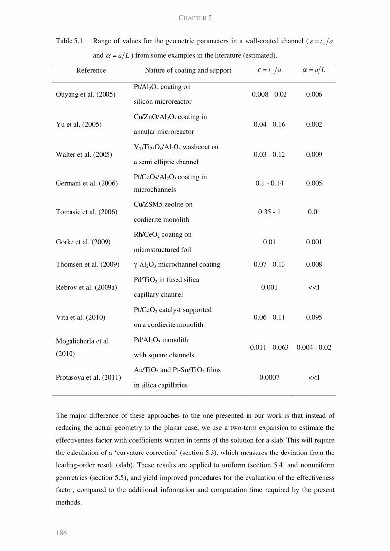
CHAPTER 5
186
Table 5.1: Range of values for the geometric parameters in a wall-coated channel (w
t aε =
and a Lα = ) from some examples in the literature (estimated).
Reference Nature of coating and support wt aε = a Lα =
Ouyang et al. (2005) Pt/Al2O3 coating on
silicon microreactor 0.008 - 0.02 0.006
Yu et al. (2005) Cu/ZnO/Al2O3 coating in
annular microreactor 0.04 - 0.16 0.002
Walter et al. (2005) V75Ti25Ox/Al2O3 washcoat on
a semi elliptic channel 0.03 - 0.12 0.009
Germani et al. (2006) Pt/CeO2/Al2O3 coating in
microchannels 0.1 - 0.14 0.005
Tomasic et al. (2006) Cu/ZSM5 zeolite on
cordierite monolith 0.35 - 1 0.01
Görke et al. (2009) Rh/CeO2 coating on
microstructured foil 0.01 0.001
Thomsen et al. (2009) γ-Al2O3 microchannel coating 0.07 - 0.13 0.008
Rebrov et al. (2009a) Pd/TiO2 in fused silica
capillary channel 0.001 <<1
Vita et al. (2010) Pt/CeO2 catalyst supported
on a cordierite monolith 0.06 - 0.11 0.095
Mogalicherla et al.
(2010)
Pd/Al2O3 monolith
with square channels 0.011 - 0.063 0.004 - 0.02
Protasova et al. (2011) Au/TiO2 and Pt-Sn/TiO2 films
in silica capillaries 0.0007 <<1
The major difference of these approaches to the one presented in our work is that instead of
reducing the actual geometry to the planar case, we use a two-term expansion to estimate the
effectiveness factor with coefficients written in terms of the solution for a slab. This will require
the calculation of a ‘curvature correction’ (section 5.3), which measures the deviation from the
leading-order result (slab). These results are applied to uniform (section 5.4) and nonuniform
geometries (section 5.5), and yield improved procedures for the evaluation of the effectiveness
factor, compared to the additional information and computation time required by the present
methods.
EFFECTIVENESS FACTOR FOR THIN CATALYTIC COATINGS
187
In section 5.6, we use the approximations to the effectiveness factor to determine the conditions
under which the channel-coating system can be considered to operate in the chemical or
diffusional regime. In many cases, this is controlled by the internal mass transfer-reaction
regimes and is important for applications such as intrinsic kinetics measurement in
microdevices and evaluation of the washcoat diffusional limitations. Finally, we evaluate an
opportunity for performance enhancement in catalytic coatings, by allowing the existence of
transverse intraparticular convection due to a pressure gradient (section 5.7). The operating
conditions under which the influence of this effect is maximized are identified.
5.2 PROBLEM FORMULATION
The reaction-diffusion equations in the catalytic coating have to be written in general for the 3
coordinates. To reduce the order of the complete model, we use the one-dimensional cylinder
model presented in section 5.2.1. The calculation of effectiveness factors from this approach is
discussed in section 5.2.2.
5.2.1 One-dimensional cylindrical model for a catalytic coating
The one-dimensional generalized cylinder model (1DGC) has been widely used for the
calculation of effectiveness factors in catalyst particles with arbitrary shape (Datta et al. 1985;
Burghardt et al. 1996; Keegan et al. 2003; Mariani et al. 2003; Mariani et al. 2008a; Mariani et
al. 2009a; Mariani et al. 2009b). The model and its assumptions are detailed in the previous
references, yielding the following form of the governing equation:
( ) ( )
2 22 2
2 2
' ' ''
1 in in
c c cc
r r r z
ε σα ε φ
ε
∂ ∂ ∂+ + =
∂ + ∂ ∂R . (5.1)
Eq.(5.1) is made dimensionless using the following normalization for dependent and
independent variables (dimensional variables are capped):
ˆ
w
r ar
t
−= ,
zz
L= and
ˆ'
in
cc
c= ; (5.2)
where w
t is the characteristic length scale in the transverse direction inside the washcoat, a is
the external diffusion length scale in the open channel, L is the channel’s length in the axial
direction and in
c is the inlet concentration per volume of washcoat (related with the channel’s
inlet concentration in
C by the porosity of the catalyst layer: in P in
c Cε= ).

CHAPTER 5
188
Figure 5.1: Geometries of the washcoats studied. (a) Uniform annular catalyst layer (circle
in circle). (b) Circle in square. (c) Square with rounded corners.
Figure 5.1 shows some common washcoat geometries and their dimensions. The reaction rate
expression can be generically expressed by
( )( )
( )
( ) ( )
( )
' 1 ' ''
1 ' '
p m
in
in p
in
c c k cc
c k c
+= =
+
V
V
RR
R, (5.3)
where the dimensional reaction rate (per unit of washcoat volume) is ( ) ( )1 2ˆ ˆ ˆ1pm
c k c k c−
= +VR
with 2'in
k k c= . The timescales for reaction (at inlet conditions) and transverse diffusion are
compared by the Thiele modulus (evaluated at the inlet),
( )2
2 w in
in
in eff
t c
C Dφ =
VR
.
Additionally, this choice of scales leads to the appearance of two geometrical parameters,
wt
aε = (transverse length scales ratio) and (5.4a)
a
Lα = (channel’s aspect ratio). (5.4b)
As discussed in section 5.1, both parameters are typically small for supported catalytic coatings.
The magnitude of ( )2
α ε measures the importance of axial diffusion, over the full length of the
washcoat, which is therefore negligible ( 1transv axial
τ τ << ). Thus, the axial dependence in the
concentration profile, results then from the concentration continuity condition at the interface :
( ) ( )' 0,surf
c r z c z= = . Normalization by surface conditions yields the following dimensionless
model:
b
a
tw,min
tw,max
dθ
x
x + d x
x = 0, 0θ =
b
a
tw,min
tw,max
I
II
( )O O,x y
tw
a
(a) (b) (c)

EFFECTIVENESS FACTOR FOR THIN CATALYTIC COATINGS
189
( )
22
2 1
d c d cc
d r r d r
ε σφ
ε+ =
+R (5.5a)
( )0 1c r = = (5.5b)
1
0r
c
r=
∂=
∂ (5.5c)
where,
( )( )
( )
' ,
surf
c r zc r
c z= (5.5d)
( )( )
( )
1
1
p
in surf m
in surf
c c Kc c
K cc
+= =
+
RR
R (with '
surfK k c= ) (5.5e)
( ) ( )2
2 2ˆ
ˆin surf w surf
in
surf surf eff
c t c
c c Dφ φ= =
VR R
(5.5f)
with ε from (5.4a). In the above equations, two parameters (w
t and σ ) are directly related with
the reduction to the one-dimensional model adopted. The success of the simplification relies on
the judicious choice of these quantities. According to the same model, w
t and σ are tied up by
an expression for the volume to surface ratio of the catalytic body . Then, the ratio between
V S for the actual geometry (where S is the area of the surface in contact with the reacting
species) and for a slab with thickness w
t (the same characteristic transverse length) is
( )( )
111 1
1w
V
t S
σ
υ εε σ
+ = = + − +
. (5.6)
For thin coatings, (5.6) expands as
( ) ( )2
3~ 1 12 6
Oσ ε ε
υ σ σ ε+ + − + . (5.7a)
Note that for an annular washcoat in a cylindrical channel: 1σ = and 1 2υ ε= + as expected. If
only the first two terms are retained in (5.7a), then a simple relationship between υ and σ is
obtained:
( )2
1σ υε
= − . (5.7b)
Thus, the problem is determined once the characteristic length for diffusion is chosen. Since this
is the length scale over which concentration decays inside the washcoat, w
t can be equal to the
maximum distance measured in the normal direction to the interface with the channel. Examples
will be given in sections 5.4 and 5.5.

CHAPTER 5
190
Eqs.(5.7) represent the simplest way of calculating σ for catalytic coatings. In the literature,
many evolved approaches have been pursed to fit σ so that more accurate predictions from the
1DGC model can be obtained. For example, Mariani et al. (2003) calculated it to fulfill the low
reaction rate asymptotics of the actual pellet. In later work from the same group, Mariani et al.
(2008b; 2009a) matched the behavior at high reaction rates. More recently, they also used
information from both regimes (Mocciaro et al. 2011), with emphasis on the prediction of
effectiveness factors in multihole and multilobe particles. According to their analysis, negative
values of their parameter σ are not likely to be obtained for catalytic pellets, but can be found
for washcoats in monolith reactors. The corrective coefficients that appear in the higher order
terms of the perturbation series for low and high φ are not useful as shape factors, in the sense
that geometries with similar behavior at high reaction rates may present significantly deviation
in the chemical regime (Keegan et al. 2005).
5.2.2 Effectiveness factor
The effectiveness factor compares the amount of reactant consumed (in the presence of
diffusional limitations) with the one that would have been converted had surface conditions
prevailed everywhere inside the catalyst. It can be calculated from
( )1
A
c dAA
η = ∫R .
According to the 1DGC model, averaging the mass balance yields
( ) ( )
1
20 0
1 11
r
d cr c dr
d r
σ
η ευ φ υ
=
−= + =∫ R . (5.8)
5.3 PERTURBATION SOLUTION FOR THIN CATALYTIC COATINGS
An approximate solution to (5.5) can be constructed by a regular perturbation method for small
values of ε . This will unfold the original problem into a sequence of (simpler) subproblems,
once the perturbation series
( ) ( )0
; n
n
n
c r c rε ε
∞
=
=∑ (5.9)
is introduced into the model and terms with the same order are collected. Generically, the
( )n
O ε subproblem is described by
EFFECTIVENESS FACTOR FOR THIN CATALYTIC COATINGS
191
( )n
O ε : ( )
2 2
200 0
1
! ! 1
n n qnqn
n n q
q
d cd c d d
d r n d n q d r d rε ε
φ ε σ
ε ε ε
−
−
== =
− = −
− + ∑
R (5.10a)
( )0 0 1c r = = and ( )0 0n
c r = = for 0n > (5.10b)
1
0n
r
d c
d r=
= . (5.10c)
The terms in the LHS of (5.10a) are dominant (diffusion in the normal direction and reaction),
while the curvature term in the RHS appears as an higher-order correction (note that this side is
annulled for 0n = ). From (5.8), a perturbation series for the effectiveness factor is also
obtained,
0
n
n
n
η η ε
∞
=
=∑ where 2
0
1n
n
r
d c
d rη
φ υ=
−= . (5.11)
In theory, one may calculate as many terms as desired (numerically or analytically when
possible). However, more terms in (5.11) may reduce the accuracy of the approximation as ε
increases and, as we will show, a two-term expansion with analytically calculated terms is
enough for our purposes.
The leading-order term from (5.10) yields the classical reaction-diffusion problem in a catalyst
slab ( a → ∞ ). Exact and approximate analytical solutions for this problem have been provided
in the literature for several forms of ( )cR (Petersen 1965; Bischoff 1967; Aris 1975; Gottifredi
et al. 1981; Gottifredi et al. 1986; Gottifredi et al. 2005a; Gottifredi et al. 2005b; Magyari 2008).
If required, numerical solution for the case of planar geometry can be obtained with
considerably less effort. Therefore, we focus on the higher-order correction that appears at
( )O ε , accounting for geometry effects.
5.3.1 Linear kinetics
When kinetics is first-order in the reactant concentration, the solution to the subproblems in
(5.10) can be obtained analytically. The leading-order term has a familiar form:
( )( )
0
cosh 1
cosh
rc r
φ
φ
− = and 0
tanh φη
υ φ= . (5.12)
Note that, this is equivalent to setting 0ε = in the original problem and therefore 1υ = , so that
0 tanhslab
η η φ φ= = (Thiele 1939; Aris 1975; Froment et al. 1979). For the subproblem
obtained when 1n = :

CHAPTER 5
192
( )( )
( )( ) ( )( )2
1 22
sinhcosh 2 cosh 2
1
rec r r r r
re
φ
φ
φσφ φ
φ
= − − + −
+ and (5.13)
22
1 2
tanh
2 2 slab
σ φ ση η
υ φ υ= = . (5.14)
According to Eq.(5.11), the two-term perturbation series for the effectiveness factor can be
written as:
( )2 2
2slab
slabO
η ε ση η ε
υ υ= + + .
Attending to the fact that for thin catalytic coatings the shape factor is given by Eq.(5.7b),
( )~ 1 1slab
slab
ηη υ η
υ + − . (5.15)
Eq.(5.15) relates the effectiveness factor for a thin catalytic coating, described by the 1DGC
model, with the one calculated for a slab catalyst, with thickness equal to the characteristic
length w
t . This dimension is one of the two pieces of information concerning geometry: the
other is the V S ratio which can be quantified explicitly for simple geometries or analyzed
digitally and measured for more complex ones. We must stress the fact that (5.15) is valid for
all values of the Thiele modulus and is not limited to high or low reaction rates. In section 5.3.2,
we understand how this relationship holds for nonlinear kinetics.
A final remark should be made to note that the 1DGC model admits an exact analytical solution
for linear kinetics. This solution is an adaptation of previous analytical work for the hollow
cylinder geometry and can be written in terms of a combination involving modified Bessel
functions with complex arguments and whose order may be integer or fractional. Naturally,
these transcendental functions aren’t of convenient evaluation and an expansion for small ε is
not easily obtained from the full solution. Moreover, the complex form of the exact solution
does not inspire an approximation for more complex situations, such as the nonlinear kinetics
examined in the next section. Apart from its simplicity, the perturbation solution has another
advantage: it writes the effectiveness factor for the actual geometry in terms of its most
elementary representation, a 1D slab.
5.3.2 Nonlinear kinetics
We would now like to understand if Eq.(5.15) holds for the case of nonlinear kinetics, with slab
η
being the effectiveness factor for a slab under the same (nonlinear) conditions experienced by
the actual geometry. In the case of first-order reactions, it is not the reaction term which

EFFECTIVENESS FACTOR FOR THIN CATALYTIC COATINGS
193
introduces complexity into the solution of the full problem. However, when kinetics is
nonlinear, an exact solution to the leading-order problem of (5.10) may not be possible or
convenient. Therefore, a perturbation scheme which affects the relative magnitude of reaction to
diffusion is required. We expect maximum deviation to appear when kinetics is comparable
with transport rates, but as we mentioned we want to avoid having to solve the 2D nonlinear
problem. Alternatively, we consider the asymptotic limits of the solution for small and large
Thiele modulus.
5.3.2.a Chemical regime
In the 1φ << limit, we look for a perturbation solution with the following form
( ) ( )2
0
; n
n
n
c r c rφ φ
∞
=
=∑ . (5.16)
This is a regular problem, where the leading order solution is naturally ( )0 1c r = , since reaction
is much slower than transverse diffusion inside the washcoat. The ( )2
O φ correction yields a
result for the effectiveness factor which is independent of the reaction rate expression ( 1η = ).
The deviation from unity is achieved in the next subproblem, where the curvature term was
retained, making the solution valid for all values of ε . With these results, the series for the
effectiveness factor becomes:
( )( ) ( )
2 1 2 4
0 0
11 ' 1nn
n r
d cO
d rη φ φ φ
υ
∞
−
= =
−= = − Λ +∑ R , (5.17)
where the coefficient Λ is only related with the shape of the coating,
( )( )
( )( ) ( ) ( )( )
( ) ( )( )( )
2 1 1 2
12
1 1 3 1 4 2 1,
1 1 1 1 3
σ σ
σ
σ ε σ ε ε ε σ
ε σ
ε ε σ σ σ
+ +
+
− + + + − + + + +
Λ = + − + − +
. (5.18)
In the limit of thin coatings, using Eq.(5.7b),
( ) ( )21
0, 1 ~3 2 3
Oε σ υ
ε σ ε
Λ → = + +
. (5.19)
For a slab catalyst ( a → ∞ ), ( )0, 1 1 3ε σΛ = = = and the expansion from Aris (1975) is
reproduced. If the limit of Eq.(5.18) when ε → ∞ is taken, then the result obtained for solid
catalyst bodies using the 1DGC model is retrieved:
( )( )( )
1,
3 1 3
υε σ
σ σ σΛ → ∞ = =
+ + +. (5.20)

CHAPTER 5
194
Note that in (5.20), υ is referred to the surface area in contact with reactants, i.e. for solid
catalyst particles, ( )1
1υ σ−
= + . The quantity Λ is related to the so called ‘first Aris number’
(Wijngaarden et al. 1998) or to the γ parameter from Mariani et al. (2003):
( )1 2
1 1
3 3An
σγ
υ υ σ σ
Λ += = = =
+ +.
The normalization proposed by Eq.(5.17) accounts for generic shape and kinetics in two
separable factors: (a) geometry effects induce a change in Thiele modulus for a slab, 2φ now
appears as 2υ φ (i.e. the characteristic length is taken as the geometric average between
wt and
V S ); (b) kinetic effects are expressed through ( )' 1R , which from Eq.(5.5e), is simply:
( )' 11
p Km
K= −
+R .
Introducing the expansion for slab
η in the chemical regime for any kinetics into Eq.(5.15) yields
( )( )
24' 1 1
1 23
Oφ
η φυ
= − − +
R
The correct factor for geometry given by (5.18) agrees with this one as 1υ → (i.e. as 0ε → )
( )22 1
~ Oυ
υ ευ
−+ .
The expansions agree up to ( )2
O ε , which is smaller than any contribution in Eq.(5.15). Thus, it
is possible to conclude that the result from section 5.3.1 is still valid for nonlinear kinetics in the
chemical regime.
5.3.2.b Diffusional regime
In the limit of a very fast reaction ( 2 1φ >> ), it is well-known that a boundary layer develops
near the interface to match the dead core (the only solution from ( ) 0c =R ) with the surface
condition (5.5b). This region is described by (5.5), with stretching of the transverse coordinate
( R r δ= , where 1~δ φ− is the thickness of the inner region):
( )
2
2
d c d cc
d R R d R
ε σ
φ ε− = −
+R ,
where the singular perturbation series for concentration writes as ( ) ( )0
; n
n
n
c R c Rε φ
∞
−
=
=∑ . The
curvature term (which accounts for geometry effects) is of ( )O ε φ , which is small in this limit
EFFECTIVENESS FACTOR FOR THIN CATALYTIC COATINGS
195
even for ~1ε . The leading-order problem resembles the reaction-diffusion in a slab, which has
been treated in a detailed manner by several authors. The analysis at this order results in a very
well-known normalization for arbitrary kinetics given by
( )
10
0 0 0
00
1 12
R
d cc d c
d Rη
φ υ φ υ=
−= = ∫R . (5.21)
This can be rewritten as 0 slabη η υ= , which is the first term from (5.15). For kinetics of the
form of Eq.(5.5e): ( )( )
( )
1
0 0 2 1
0
11 , ,2 ,
1
p
Kc d c F m p m K
m
+= + + −
+∫R with 1m > − or simply
( )1 2
1 m−
+ for power-law kinetics.
To obtain an higher order term capturing the effect of geometry, we follow Wedel and Luss
(1980) to write the solution of
0
201
12c
d cd c dc
d R dc d Rε σ− = −
R
as 0
0
0
010
0 10 0
c
cR R
d cd cd c
d R d c d R d R
ε σ→
→= =
=
∫ .
We make the following approximation in the boundary layer:
( ) ( ) ( )0 00 0 0
00
~RR
d c d cc dR c dR c
d R d R
∞ ∞
=
= ∫ ∫R R R ,
which yields the following two term solution for the effectiveness factor:
( ) ( ) ( )1 1
30 0 0 02
0 0
12 c d c c d c O
ε ση φ
φ υ φ υ
−= + +∫ ∫R R . (5.22)
In terms of the kinetically generalized Thiele modulus (independent of shape) defined by
Petersen (1965), Bischoff (1967) and Aris (1975)
( )
1
0 0
0
2 c d c
φΦ =
∫R, (5.23)
Eq.(5.22) writes as
( ) ( )3 3
2 2
1 1 1 1 1
2O O
ε σ υη φ φ
υ υ υ υ
− −−= + + = + +
Φ Φ Φ Φ. (5.24)
Since in this limit a slab with arbitrary kinetics is described by 1slab
η = Φ , Eq.(5.15) is
recovered. The separable geometric factors coincide with our analysis in section 5.3.1.

CHAPTER 5
196
5.3.2.c Monotonous ( )2
η φ curves (“normal” kinetics)
Since Eq.(5.15) holds for nonlinear kinetics in the chemical and diffusional regimes even at
higher orders ( ( )2
O φ and ( )2
O φ− , respectively), we can expect the intermediate region to be
described at least approximately by the same equation. However, it is known from other shape
normalizations that maximum deviation is found when ~ 1φ . Also, the error of the
approximation increases when kinetics present strong inhibition or multiplicity effects (Keegan
et al. 2003). In this work, we address the case of ‘monotonous ( )2
η φ curves’, where reaction
rate is an increasing function of the reactant’s concentration.
The solution requires the calculation of the effectiveness factor for the nonlinear reactive slab,
which can be solved numerically with considerably less effort than the original problem.
Approximations are also available (Gottifredi et al. 1981; Gottifredi et al. 1986; Haynes Jr 1986;
Wijngaarden et al. 1998; Gottifredi et al. 2005a; Lee et al. 2006). Here we present a different
derivation in terms of a generalized Thiele modulus with respect to kinetics, which should be
introduced into a function which fulfills the asymptotic limits for a slab. We choose the simple
solution for first-order reaction,
( )tanh
slabη
ΦΦ =
Φ, (5.25)
where the normalized Thiele modulus with respect to kinetics Φ is:
( )( )
112 2
0 02 2 20
' 12
1 1c d c
φ
φ φ φ
−
Φ= +
+ + ∫
RR . (5.26)
As expected, φΦ = when the reaction is first-order. For power-law kinetics,
2 2
2 2 2
1
1 2 1
m m φ
φ φ φ
Φ += +
+ +. (5.27)
We note that our normalization includes the classical result from Petersen (1965) and Bischoff
(1967), which is more rigorous as φ → ∞ . However, (5.27) predicts the effectiveness factor in
the intermediate and low range of φ much better. For a slab geometry, introducing the
generalized Thiele modulus into Eq.(5.25) results in comparable result to the empirical
correlation from Gottifredi et al. (1986) particularly for 1m > (around 0.55% maximum error
for 2m = ). Our result is particularly better than the existing approximate solutions for low m
(even though the maximum error also increases as the order of reaction becomes lower than 1).
The effectiveness factor is predicted by (5.25) with less than 1% error (for 3 4m = ) and less
than 2.6% for 1 2m = . As 0m → , the transition between asymptotes becomes much sharper
and the smooth transition from our normalization becomes less accurate (5.3% error for 1 3m =

EFFECTIVENESS FACTOR FOR THIN CATALYTIC COATINGS
197
and 7% for 1 4m = ). In those cases, a better approximation may be obtained by combining
both limits in a powered addition as
2 2
2 2 2
1
1 2 1
b bb
m m φ
φ φ φ
Φ += +
+ + (5.28)
with 1b > . We do not consider b a fitting parameter, since the final result is pretty insensitive
to virtually any value chosen, provided that it is reasonably higher than 1. In the cases
examined, the maximum error changes from 3.38% to 3.44% when b changes from 2 to 100
(for 1 3m = ). The same observation holds for 1 4m = (maximum error 3.7% at least for
2b ≥ ).
Wijngaarden et al. (1998) compared several modified Thiele modulus that bring the
effectiveness factor curves together for several reaction kinetics in the low and high region of η
(equivalently, the zero-th and first Aris numbers). Approximations in these two limits are also
given, but with excessive error in the intermediate range. A better estimate using information
from both asymptotes is proposed, but it requires an iterative procedure. For a first-order
reaction, the maximum error is 2.2% for a slab. They also used the same formula for the hollow
cylinder, with maximum error of 4.4%. Generally, other approximations are of less convenient
evaluation or have higher errors associated than the one proposed.
For this case, the effectiveness factor for slab geometry is always expected to be less than 1.
Then from Eq.(5.15): 1 1slab
υ η η−
< < . The maximum deviation from the slab geometry is
1 ~2
slabη η ε σ
υη
−= − . (5.29)
For 0.1ε = , a cylindrical catalyst coating deviates from the slab geometry by approximately
5%. Eq.(5.29) allows an estimate of the maximum thickness admissible for the actual geometry
to be represented by a slab, for a specified amount of relative error. Note that for “abnormal
kinetics” (with inhibiting or nonisothermal effects), the analysis predicts that at least for some
values of the Thiele modulus where 1slab
η > , it is possible that 1slab
η η > . In these cases,
advantage from using thicker coatings may exist.
5.3.3 Egg-shell catalysts
If the internal core of a pellet consists in a nonporous/inert solid ( ˆ0 r a≤ ≤ ), with the catalytic
material only in an outer layer ( ˆw
a r a t≤ ≤ + ), then a similar problem is obtained but with
reverse boundary conditions on both surfaces, given by
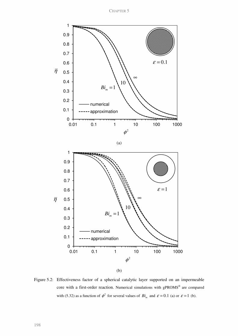
CHAPTER 5
198
(a)
(b)
Figure 5.2: Effectiveness factor of a spherical catalytic layer supported on an impermeable
core with a first-order reaction. Numerical simulations with gPROMS® are compared
with (5.32) as a function of 2φ for several values of
mBi and 0.1ε = (a) or 1ε = (b).
0
0.1
0.2
0.3
0.4
0.5
0.6
0.7
0.8
0.9
1
0.01 0.1 1 10 100 1000
numerical
approximation
η
2φ
0.1ε =
1m
Bi =10
∞
0
0.1
0.2
0.3
0.4
0.5
0.6
0.7
0.8
0.9
1
0.01 0.1 1 10 100 1000
numerical
approximation
η
2φ
1ε =
1m
Bi =
10
∞

EFFECTIVENESS FACTOR FOR THIN CATALYTIC COATINGS
199
( )1 1c r = = (5.30a)
0
0r
c
r=
∂=
∂ (5.30b)
The surface reaction is now referred to the external surface and the effectiveness factor
becomes:
2
1
1
r
d c
d rη
φ υ=
= , where ~ 12
ext w
V
S t
ε συ = − as 0ε → . (5.31)
The shape exponent σ is used in the reaction-diffusion equation as in (5.1). The reference to the
outer surface yields a change in the sign associated with σ , and this is why in the 1DGC model
for washcoats: 0σ < (Keegan et al. 2005). Following our perturbation procedure as outlined in
section 5.3.1, Eq.(5.15) is found to still apply as long as υ is defined as in (5.31).
An asymptotic solution at the diffusional regime according to (5.23) is known for several kinetic
expressions arising in enzymatic reactions occurring in pellicular catalysts (Horvath et al. 1973;
Vos et al. 1990). There isn’t any reason for the results in section 5.3.2 not to be valid for egg-
shell catalysts and therefore (5.15) can be used for some nonlinear kinetics, as discussed
previously. If external mass transfer resistance is also considered, then the approximate
expressions for the effectiveness factor are more complex. We can also show that in the case of
finite external mass transfer, Eq.(5.15) is again obtained (the superscript – denotes reference to
bulk fluid conditions)
( )1 1slab
slab
ηη υ η
υ= + − , (5.32)
with the well-known solution for a slab with linear kinetics (Aris 1975),
2 cothm
slab
m
Bi
Biη
φ φ φ=
+.
The mass Biot number for external mass transfer is given by m m w eff
Bi k t D= . For a spherical
geometry, 2σ = and 2
2
1 3~ 1
1 2
ε ευ ε
ε ε
+ += −
+ +, the effectiveness factor predicted from (5.32) is
compared with numerical results in Figure 5.2, when a first-order reaction is occurring.
5.4 UNIFORM ANNULAR COATING
The simplest case possible, apart from the slab catalyst layer, is the one of an annular washcoat.
Uniform annular catalyst layers are found when a circular channel is perfectly coated or in the
case of egg-shell catalysts in noncircular channels (Kreutzer et al. 2006).
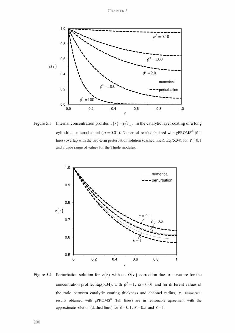
CHAPTER 5
200
Figure 5.3: Internal concentration profiles ( )c r ˆ ˆsurf
c c= in the catalytic layer coating of a long
cylindrical microchannel ( 0.01α = ). Numerical results obtained with gPROMS® (full
lines) overlap with the two-term perturbation solution (dashed lines), Eq.(5.34), for 0.1ε =
and a wide range of values for the Thiele modulus.
Figure 5.4: Perturbation solution for ( )c r with an ( )O ε correction due to curvature for the
concentration profile, Eq.(5.34), with 2 1φ = , 0.01α = and for different values of
the ratio between catalytic coating thickness and channel radius, ε . Numerical
results obtained with gPROMS® (full lines) are in reasonable agreement with the
approximate solution (dashed lines) for 0.1ε = , 0.5ε = and 1ε = .
0.0
0.2
0.4
0.6
0.8
1.0
0.0 0.2 0.4 0.6 0.8 1.0
numerical
perturbation
2 0.10φ =
2 1.00φ =
2 10.0φ =
2 100φ =
2 2.0φ =
r
( )c r
0.5
0.6
0.7
0.8
0.9
1.0
0 0.2 0.4 0.6 0.8 1
numerical
perturbation
0.1ε =
0.5ε =
1ε =
( )c r
r
EFFECTIVENESS FACTOR FOR THIN CATALYTIC COATINGS
201
In the latter situation, the channel is first modified by introduction of a low BET material
coating, which blocks the macroporosity of the channel walls and rounds the shape of the
channel, filling the poorly used regions. Pérez-Cadenas et al. (2005) have shown the superior
performance of these catalysts in the hydrogenation of fatty acid methyl esters compared with a
square channel cordierite monolith. Better utilization and distribution of the catalytic layer was
observed, as well as higher selectivity to the desired products. This case can also appropriately
model diffusion and reaction in Raschig rings and hollow cylinders with internal flux (Mariani
et al. 2003), in the limits of small aspect ratio (w
t L<< ).
This shape is schematically represented in Figure 5.1a and has very well-defined geometric
characteristics:
wt = thickness of the annular catalyst layer (5.33a)
12
ευ = + (5.33b)
and therefore 1σ = .
5.4.1 Linear kinetics
According to the results presented in section 5.3.1, the internal concentration profile and the
effectiveness factor curve are given by:
( )( )
( )( )( ) ( )
( )( )
22
22
cosh 1 sinh; cosh 2 cosh 2
cosh 1
r rec r r r r O
re
φ
φ
φ φε ε φ φ ε
φ φ
− = − − + − +
+
(5.34)
( )2
22
1 tanh tanh
1 2 2O
φ ε φη ε
ε φ φ
= + +
+ . (5.35)
The two-term expansion (5.34) is plotted in Figure 5.3 for 0.1ε = and several values of 2φ
(from 0.1 to 100). The inclusion of the second term reduces the maximum relative error from
0.16% to 0.004% for 2 0.1φ = and from near 5% to less than 0.1% when 2 100φ = (in the
region of virtually zero concentrations, corresponding to absolute error of 810− ). Figure 5.4
compares the performance of the approximation for several values of the perturbation parameter
ε . Naturally, better agreement is obtained as 0ε → , but even for values as high as 1ε = the
maximum error reduces from around 10% to 3%, when the ( )O ε correction is added.

CHAPTER 5
202
Figure 5.5: Magnitude of the ( )O ε correction to the transverse concentration profile in a slab
coating due to the weak presence of curvature.
Figure 5.6: η vs. 2φ curve for a long catalytic annular region ( 0.01α = ) for 0.1ε = , 0.5ε =
and 1ε = . Numerical results are in good agreement with perturbation series given by
Eq.(5.35).
0
1
2
3
4
5
6
7
8
9
10
0.0 0.2 0.4 0.6 0.8 1.0
2 0.10φ =
2 2.0φ =
2 10.0φ =
2 100φ =
2 1.00φ =
r
( )2
1 10c r ×
0.1
1
0.01 0.1 1 10 100
numerical
perturbation
0 .1ε =
0.5ε =
1ε =
η
2φ
EFFECTIVENESS FACTOR FOR THIN CATALYTIC COATINGS
203
The ( )1c r term in Eq.(5.34) is negative and its absolute value register a maximum, except for
low φ (where ( )1c r is maximum at 1r = ). The curvature importance increases with the
distance from the interface, as long as reasonably high transverse concentration gradients are
present. The position where the correction is maximum maxr marks the transition from a region
of high transverse gradients to another where the concentration profile starts to flatten out. For
1φ > , maxr is the reactant penetration length ( 1φ
− ). The η vs. 2φ curve is plotted in Figure 5.6
with less than 3% maximum relative error for 1ε = and only around 1% for 0.1ε = , compared
to numerical results. We note that other methods in the literature for calculating the
effectiveness factor have some drawbacks compared with our approach, namely: (a) the use of
the geometrical Thiele modulus in tanhg g
η φ φ= leads to considerable high errors in the
intermediate range of φ ; (b) analytical results from Lewis et al. (1974) and Wijngaarden et al.
(1998) imply the inconvenient evaluation of modified Bessel functions or infinite series of these
functions; (c) the 1DGC solution for the effectiveness factor (Burghardt et al. 1996) with a
value of σ fitted to the chemical regime is again written in terms of Bessel functions (with
fractional or integer orders) with (Mariani et al. 2003):
( ) ( )( ) ( ) ( )
( ) ( )( ) ( ) ( )
42
42
2 6 2 9 4 2 12 1 ln 1
2 2 2 3 4 2 4 1 ln 1
ε ε ε ε ε ε ε ε
σ
ε ε ε ε ε ε ε ε
− + + + + + + + + =
+ + + + + − + +
,
and 0.4ε < so that the error does not exceed 0.7%. Therefore, our method is simple, its
evaluation is convenient, does not require fitting to any particular regime (it is valid for the
whole range of φ ) and is accurate.
5.4.2 Nonlinear kinetics
The treatment for nonlinear kinetics follows the analysis in section 5.3.2. As discussed there, the
effectiveness factor depends on υ (here given by Eq.(5.33b)) and on slab
η (calculated
numerically or with Φ in Eq.(5.25)), according to (5.15). Table 5.2 shows the maximum
deviations observed between our solution and the numerical calculations for some kinetic forms.
The reaction-diffusion problem was solved numerically with DASOLV routine from gPROMS®
with discretization of the spatial coordinate r by orthogonal colocation in finite elements. The
polynomial was second order and 1000 elements (first-order reaction) or 500 elements
(remaining kinetics) were used. As expected, the factors that contribute to an increase in the
relative deviation are: increase in the coating thickness (ε ), intermediate values of Thiele
modulus ( 2 ~ 1 10φ − ) and ‘abnormal kinetics’ (the two last cases in Table 5.2), where the
approximation is only acceptable for lower values of ε .
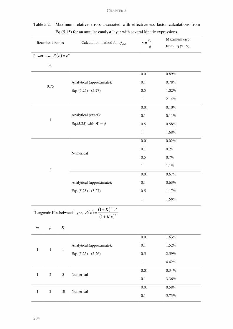
CHAPTER 5
204
Table 5.2: Maximum relative errors associated with effectiveness factor calculations from
Eq.(5.15) for an annular catalyst layer with several kinetic expressions.
Reaction kinetics Calculation method for slab
η wt
aε =
Maximum error
from Eq.(5.15)
Power-law, ( )m
c c=R
m
0.75 Analytical (approximate):
Eqs.(5.25) - (5.27)
0.01 0.89%
0.1 0.78%
0.5 1.02%
1 2.14%
1 Analytical (exact):
Eq.(5.25) with φΦ =
0.01 0.10%
0.1 0.11%
0.5 0.58%
1 1.68%
2
Numerical
0.01 0.02%
0.1 0.2%
0.5 0.7%
1 1.1%
Analytical (approximate):
Eqs.(5.25) - (5.27)
0.01 0.67%
0.1 0.63%
0.5 1.17%
1 1.58%
“Langmuir-Hinshelwood” type, ( )( )
( )
1
1
p m
p
K cc
K c
+=
+
R
m p K
1 1 1 Analytical (approximate):
Eqs.(5.25) - (5.26)
0.01 1.63%
0.1 1.52%
0.5 2.59%
1 4.42%
1 2 5 Numerical 0.01 0.34%
0.1 3.36%
1 2 10 Numerical 0.01 0.58%
0.1 5.73%

EFFECTIVENESS FACTOR FOR THIN CATALYTIC COATINGS
205
5.5 NONUNIFORM COATINGS
The best method to deal with the calculation of the effectiveness factor in nonuniform coatings
appears to be the so-called ‘slice method’ from Papadias et al. (2000a; 2000b). Briefly, the
domain is divided into a series of slices, then the average effectiveness factor is calculated from
the mass/volume weighed summation of all pieces and is given by
1
N
i i
i
wη η
=
=∑ . (5.36)
The method was applied to several geometries (Papadias et al. 2000a; Papadias et al. 2000b;
Hayes et al. 2005) and was also included in monolithic reactor simulation (Gonzo 2008; Gonzo
et al. 2011). However, so far each slice has been treated as a slab, and i
η calculated
accordingly, referred to the geometric characteristic length.
We propose a modification to the method, which consists in calculating i
η from Eq.(5.15). This
introduces another parameter into the model, the characteristic length for diffusion of each slice,
which together with the volume-to-surface ratio characterizes each segment i :
,w it = maximum transverse distance normal to the interface in i (5.37a)
,
i
i
w i i
V
t Aυ = . (5.37b)
The volume fraction of each slice is i i
w V V= and i
A is the fluid-solid interfacial area. The
original treatment assumes 1i
υ = and ( ),i slab i iη η φ= , with
iφ referred to ,w i
t .
5.5.1 Circular channel in square geometry
An extreme case of nonuniform deposition of washcoat in a rectangular channel is the ‘circle in
square’ geometry, depicted in Figure 5.1b. The dimensionless local thickness in terms of the
angular coordinate is
( )( )
( )min1 sec 1wt
a
θε θ ε θ= = + − ,
where min ,minwt aε = and due to symmetry of this geometry, 0 4θ π≤ ≤ . A differential slice i
corresponding to an angular change of dθ has the following geometric features, according with
Eqs.(5.37):
( ) ( ), secw i w
t t d b d aθ θ θ θ= + = + − (5.38a)

CHAPTER 5
206
Figure 5.7: Error of several calculation methods for the effectiveness factor relative to the
result obtained with a 2D numerical solution from Hayes et al. (2005) for several
values of the Thiele modulus 2g
φ . The washcoat geometry is a circle in square (Figure
5.1b) and first-order kinetics is considered. The approximate methods used to estimate η
include: the conventional ‘slice method’ used by Hayes et al. (2005) and with 100 slab
slices; and Eqs.(5.36) and (5.38) for 50 and 100 curved slices.
( )2
, ,
tan tan1
2 2i
w i w i
ddV dA b a
t t a d
θ θ θυ
θ
+ − = = −
. (5.38b)
Eq.(5.38a) expresses a scaling for the transverse coordinate, where its value is normalized by
the maximum value registered inside a slice (this occurs on the upper value taken by θ ).
Assuming (as in previous literature) that the slices are equally parted (all slices have the same
dθ ):
( )2 2
2 2
tan tan
4i
b d a ddVw
V b a
θ θ θ θ
π
+ − − = =
−. (5.38c)
The conventional ‘slice method’ treats each slice as a slab with ,w it dV dA= and 1
iυ = ,
whereas Eqs.(5.38) add a curvature correction to each segment. Figure 5.7 compares several
approximate methods for calculating the effectiveness factor with the 2D numerical solution
0.0
0.5
1.0
1.5
2.0
2.5
3.0
3.5
4.0
4.5
0.01 0.1 1 10 100
Lc geom (Hayes, 2005)
100 slab slices
50 curved slices
100 curved slices
2g
φ
err
or
rela
tive t
o 2
D n
um
erical solu
tion %

EFFECTIVENESS FACTOR FOR THIN CATALYTIC COATINGS
207
(finite element method) from Hayes et al. (2005). For a square with 0.5 mmb = and
min 0.021ε = , the conventional slice method was also employed by Hayes et al. (2005) (using
the geometrical characteristic length). We add the result for 100 slab slices for comparison, as
well as the calculation from Eqs.(5.36) and (5.38) for 50 and 100 curved slices.
We can observe that the number of slices required to achieve a desired level of accuracy
decreases sharply when the curvature effect of each slice is taken into account. The
improvement is particularly noticeable in the intermediate region of Thiele modulus, where 50
annular slices have less than half the error associated compared to 100 slab slices. The level of
effort added by our approach is negligible and the improvement is significant, even for the
simpler case of linear kinetics. Hayes et al. (2005) also report another approach, which however
requires a preliminary step of numerical evaluation, and has higher error associated in the
intermediate region (comparable with 100 slab slices).
5.5.2 Square channel with rounded corners
This geometry is closer to the actual geometries found in practical cases, where the washcoat
accumulation is more pronounced only at the corners. Chou and Stewart (1986) considered this
shape and performed numerical calculations with external mass transfer resistance. Papadias et
al. (2000b) and Hayes et al. (2005) calculated the effectiveness factor using the slice method,
where each section was treated as a slab. We divide the geometry (see Figure 5.1c ) into two
domains: a planar one characterized by a uniform (minimum) thickness (domain I in Figure
5.1c), and a circular fillet with center at ( ),x x and where the washcoat thickness increases
(shown as domain II). Due to symmetry, the angular coordinate in domain II is 0 4θ π≤ ≤ .
Each domain and slice i (a section of II between θ and dθ ) is described by:
( )
,min
, ,min
domain
domain cos
w
w i w
t
t t aa
dθ θ
= +−
+
I
II (5.39a)
( ) ( )
( ) ( )
2
min
min
1 domain
1 tan tan1domain
2 1 sec 1
i d d
d d
υ ε θ θ θ θ
θ ε θ θ
= + + − −
+ + −
I
II (5.39b)
( )
( ) ( )
( ) ( )
( ) ( )
min min2
min min min
2
min
2
min min min
2 1domain
2 1 1 4
1 tan tandomain
2 1 1 4
iw
d d
ε β ε
ε β ε ε π
ε θ θ θ θ
ε β ε ε π
− −
− − + + −
= + + − −
− − + + −
I
II
(5.39c)
CHAPTER 5
208
where the ratio between the radius of the rounded corner and the half side of the square channel
is b aβ = and the minimum dimensionless thickness is min ,minwt aε = . Domain I is treated as a
single slice, while the number of slices taken to describe domain II is chosen so that
4slices
N dπ θ= . Both contributions are added according to
, ,1
Nslices
I I i II II i
i
w wη η η
=
= + ∑ , (5.40)
where ( ),minI slab wtη η= and ( ), ,
II i slab iη η υ is the effectiveness factor for an annular slice, given
by Eq. (5.15). One of the geometries studied by Papadias et al. (2000b) has the following
geometric features: min 0.056ε = , 1.39β = and 0.36 mma = . For a first-order reaction, they
considered 30 planar slices but also solved the reaction – diffusion 2D problem numerically
(finite element method with an uniform mesh of 8640 triangular elements for 0.2η > , and an
adaptive mesh with maximum of 90 000 elements for low η ). A maximum error of 4.9% was
reported, which occurs in a temperature range between 450 and 500 K. We compare the solution
obtained with 30 annular slices in Eq.(5.40): in the same range, the maximum error observed is
1.5%. Hayes et al. (2005) presented results for this geometry with min 0.030ε = , 1.44β = and
0.347 mma = . With respect to their 2D numerical solution, a maximum error of 1.6% is
observed with 100 annular slices, while 3.6% deviation occurs when planar slices are
considered. In both cases, the inclusion of the ( )O ε correction, improves the solution.
It should be further noted that: (a) the errors tend to decrease when the fraction of washcoat
described by a planar wall with uniform thickness increases (i.e. maximum errors are observed
for the case of circular channel in square geometry) and (b) in principle, the improvement in the
results is also valid for nonlinear kinetics, where the effectiveness factor in a slab geometry is
calculated either numerically or by the approximation in section 5.3.2.c.
5.6 INTERPLAY BETWEEN INTERNAL AND EXTERNAL MASS TRANSFER – REACTION
REGIMES
The delimitation of the regimes arising from the interaction between mass transfer and reaction
appears in the literature in a number of ways, most of them equivalent. We use the concentration
gradient at the catalytic surface to evaluate the extension of mass transfer limitations. This is
rigorously related to the effectiveness factor for arbitrary kinetics, according to Eq.(5.8). A
scaling relationship is obtained from this condition: 2 1η φ << for kinetic control and 2 1η φ >>
for diffusional control, which reproduces the Weisz-Prater criterion for catalytic pellets (Weisz
et al. 1954).

EFFECTIVENESS FACTOR FOR THIN CATALYTIC COATINGS
209
The effectiveness factor is an average of the reaction rate inside the catalytic layer referred to
surface conditions. For a first-order reaction,
surf
c
cη = . (5.41)
Moreover, the internal regimes are related with the external ones by the flux continuity
condition:
01
'
ch
effch
ch rr
Dc c
r D rε==
∂ ∂=
∂ ∂, (5.42)
where the dimensional variables in the channel are ˆch ch in
c c C= and ˆch
r r a= ; and D is the bulk
fluid diffusivity. The parameter which governs the magnitude of internal and external mass
transport limitations is
2
effD Da
Dε η φ υ= , (5.43)
where Da is the Damköhler number for a wall-coated microchannel reactor. If a concentration
boundary layer with thickness δ develops at the channel’s inlet regime, then the rescaled
Damköhler number is appropriate ( *Da Da δ= ) (Chapter 4). In terms of timescales for internal
and external diffusion, 2int ext eff
D Dτ τ ε= .
For the external (channel) domain, we have used the concept of the degree of mass transfer
control θ (Chapter 4), which is related to the ratio between the average concentration in the
channel and its surface value:
1ch
surf
ch
c
cθ = − . (5.44)
The value of this parameter ranges from 0 in the external kinetic limit to 1 under severe mass
transfer limitations.
Frequently, the criteria are given in terms of operating variables, e.g. the temperature above
which diffusional effects are present in a particular system. Under some assumptions, the
criteria formulated in dimensionless manner can be rewritten explicitly for the relevant
quantities characterizing geometry and operation. In the definitions of both Thiele modulus and
Damköhler’s number, the temperature dependence of the time constant for reaction (evaluated
at the surface) is written as
( ) ( )
00
ˆ ˆ1 1~ exp lim
ˆ ˆsurf surf
T Tsurf G surf
c cE
c R T T c→
−−
V VR R
,
CHAPTER 5
210
where 0T is a reference temperature, E is the activation energy and G
R is the ideal gas
constant. When kinetics is of ‘power-law’ type, 0T → ∞ is a convenient choice and
( )( )
1
0
ˆˆ~
ˆG
E
msurf R T
surf
surf
ck c e
c
−
−VR
,
where 0k is the pre-exponential factor in the Arrhenius law. In more complex kinetics, with
other temperature-dependent constants, 0T should be chosen at a value in the range predicted by
the expressions below. The same applies to the calculated values of diffusivity, but if required a
simplified iterative procedure may be used. If all the correct dependences need to be considered,
then the problem is still reduced and consists in solving a nonlinear algebraic equation, instead
of the full convection-diffusion-reaction problem at both channel and washcoat domains.
5.6.1 Kinetic regime
We now discuss the operating boundary for the kinetic regime for different magnitudes of
( )effD Dε , i.e. change in the controlling behavior from internal to external mass transfer.
5.6.1.a External mass transfer faster than internal diffusion
If the effective diffusivity in the catalyst layer is much smaller than the bulk diffusivity (for
example, in some zeolite washcoats) and the coating is not extremely thin, then it is likely that
( ) 1eff
D Dε << . This means that internal diffusion is the rate-limiting step. Therefore, it is
possible that no external mass transfer limitations are observable in the channel, but internal
concentration gradients exist. For the whole phenomena to be under kinetic control the
following condition is sufficient (from (5.43), Da is even smaller): 2 1η φ υ << .
For a specified value of the effectiveness factor (close to unit) given by Eq.(5.17), and
considering Arrhenius-type temperature dependence only in the kinetic constant k yields the
following expression
20ln
1
GE R
Tη
η
≤ Φ Λ
−
, (5.45)
as the temperature range for which the washcoat (and hence the channel) is free from mass
transport limitations. In (5.45), the temperature independent Thiele modulus is defined as
EFFECTIVENESS FACTOR FOR THIN CATALYTIC COATINGS
211
( ) ( )0
0
220
ˆlim
ˆG
surf E R Tw
T Teff surf
cte
D cφ
→
=VR
and (5.46a)
( )2 20 0' 1 φΦ =R . (5.46b)
The shape factor is defined in (5.18), but for thin catalytic coatings is simply 3υΛ = . For
power-law kinetics associated with only one constant, (5.46a) is simply
( )12 2
0 0 ˆm
w surf efft k c Dφ
−
= .
Joshi et al. (2010) simulated numerically the oxidation of CO in a circular channel with first-
order kinetics. The values reported for diffusivities and geometric characteristics yield
( ) ~ 0.24eff
D Dε . In these conditions, the temperature below which kinetically controlled
conditions prevails is according to (5.45): 187ºCTη
≤ ( 0.91η ≥ ). The simulations performed by
these authors in channels with different lengths showed very weak dependence of the
temperature for kinetic control on the channel dimension ( L from 0.01 to 10 cm), with variation
between 189ºC and 185ºC, approximately. Our estimate is therefore very reasonable (maximum
1% relative error) given the assumptions, and circumvent the need for numerical solution of the
channel-washcoat problem for an extended range of parameters and the rejection of the values
which do not lead to the specified η and θ (or alternatively, the need for iterative calculation).
Groppi et al. (2001) studied the kinetics of methane combustion in an annular microreactor with
a surface coated with a PdO/Al2O3 catalyst layer. They found up that the limiting condition for
intrinsic kinetics evaluation was internal diffusion and this could only be achieved by keeping
10 µmw
t ≤ (so that the effectiveness factor is kept above 0.9). The same qualitative conclusion
can be reached taking their data and calculating according to (5.43):
0.19effD
Dε≤ . (5.47)
Note that in (5.47), ε is the ratio between the catalyst layer thickness and the gap between outer
and inner cylinders radii, while the importance of curvature should be evaluated by another
parameter (defined as the catalyst thickness divided by the inner cylinder radius). In their
conditions, for effectiveness factor greater than 0.9 and ~ 10 µmw
t , the maximum temperature
for kinetic control from (5.45) is 854KTη
≤ ( 581ºC ).
The temperature in their simulations was 873K and the effectiveness factor is higher than 0.9 if
9 µmw
t ≤ micrometers, which is in good agreement with their simulations. Therefore, we may
expect that their measurements up to about 600ºC, are free from diffusional limitations in line
with their predictions. Note that the geometrical parameter in this case is defined as
2
2 2in w
in w
r t
r tυ
+=
+

CHAPTER 5
212
where in
r is the radius of the internal cylinder in which the catalyst layer with thickness w
t is
supported.
As seen above, the relevant condition in practice for attaining kinetic regime in both domains is
not related with channel characteristics. Therefore, the usual strategy of working at high
flowrates to ensure kinetic control in the channel (or decrease its length) will not sort much
effect in this case. This can be noticed from the numerical solution of the problem, since near or
in developing profile conditions, the limiting temperature remains unaffected. We note that
when Da is small, the parameter which governs the regime definition in the channel at
developing concentration profile conditions ( *Da ) is even smaller (since it appears multiplied
by the normalized thickness of the boundary layer, 1δ << ).
Figure 5.8: Effect of temperature-dependent effective diffusivity on the kinetic regime
boundary. The solution involving the Lambert W function Eq.(5.49) is shown for
0 10γ = and several values of the power w in (5.48). The limiting coordinates below
which real values are not obtained are depicted by ○. The approximation in (5.50) and the
result for 0w = from (5.48) are also represented.
0
0.1
0.2
0.3
0.4
0.5
0.6
0.7
0.8
0.9
1
1 10 100 1000 10000 100000 1000000
Lambert W function solution
approximation
102 103 104 105 106
0w =
0.5=
1=1.5=
2=
GT R
E
η
( )20 1 ηΦ Λ −

EFFECTIVENESS FACTOR FOR THIN CATALYTIC COATINGS
213
If the effective diffusivity also presents a pronounced temperature dependence given by
,0 0
w
eff
eff
D T
D T
=
, (5.48)
an estimate for Tη
is still possible in terms of the Lambert W function from Mathematica® or
Matlab®,
1/
20 0
1
G
w
G
E RT
EwW
R T w
η
η
≤ − − −
Φ Λ
(5.49)
which requires numerical evaluation and yields real values for ( ) ( )20 01
w
e wη γΦ Λ − > . An
approximate solution is obtained if the dependence in (5.48) is recognized to be subdominant
compared with the one expressed by Arrhenius law for the kinetic constant. This is constructed
in an iterative manner, with (5.45) as a starting point and writes as
2 20 0 0ln ln ln
1 1
G
G
E RT
R Tw
E
η
η η
≤ Φ Λ Φ Λ
+ − −
. (5.50)
Note that in Eqs.(5.49) and (5.50), eff
D in (5.46a) is evaluated as ,0effD . The same approximate
treatment can apply to the case where other kinetic constants exhibit strong temperature
dependence, e.g. K in Eq.(5.5e). For a fixed value of ( )0 0GE R Tγ = ,
GT R E can be plotted
as a function of ( )20 1 ηΦ Λ − for several values of w . The results from Eqs.(5.45), (5.49) and
(5.50) are plotted in Figure 5.8 for 0 10γ = . Our approximate expression (5.50) is valid for weak
( )effD T dependences (low values of w ) and high ( )
20 1φ ηΛ − . Actually, for
( )20 1 1ηΦ Λ − >> , which is the case since 1η → and 2 2
0 limT
φ φ→∞
= is usually large, this effect is
negligible and the results are well described by (5.45). The typical diffusion mechanism inside a
washcoat usually yields values of ~ 0.5w . We also note that in this regime, ( ) 1eff
D Dε << , so
the magnitude of the effective diffusivity is expected to be low. Moreover, the effect loses
relevance if the reaction activation energy is large. The net result from considering temperature
dependence of diffusivity is to increase the temperature below which kinetic control prevails.
Therefore, strong dependence of the effective diffusivity on temperature is useful for kinetic
measurements.
CHAPTER 5
214
5.6.1.b Internal diffusion faster than external mass transfer
If ( ) 1eff
D Dε >> (e.g. in the limit of an extremely thin washcoat), then from (5.43)
2Da η φ υ>> , and it is possible to observe limitation in the interphase mass transfer to a
catalytic coating controlled by kinetics. In this case, it suffices to require the negligibility of
concentration gradients in the channel. In Chapter 4, we have provided correlations for θ of the
form: ( ),m
Da f Pe zθ α= , where m
Pe zα is Graetz’s parameter ( ( )2
mPe a u L Dα = ).
Alternatively, a uniformly valid solution for Sherwood number with Neumann boundary
condition at the wall could be used. We are going to consider the case of fully developed
laminar flow inside a circular channel, however the analysis is similar for the other cases
discussed in Chapter 4 and can be easily generalized. Ignoring the temperature dependence on
parameters other than the kinetic constant k , the reference Damköhler number writes as
( ,0 0surf wk k t υ= ):
( ) ( )0
0
,00
0
ˆlim
ˆG
surfsurf E R T
T Tsurf
ck aDa e
D k c→
=VR
. (5.51)
Note that since internal transport is very fast, 1η → . The temperature below which kinetic
controls is
( ) 30
0
ln 1 1 24ln ln 1.033
11
G G
nn
n m
E R E RT
Da Da PeDa
n z
θ
αθ
θ
= = −
− +
. (5.52)
The coefficient n takes the value of 4 for laminar flow and the degree of mass transfer control
θ should be set to a low value (kinetic conditions). The following limits of (5.52) can be
obtained
011ln
24
GE R
TDa
θ
θ
=
(fully developed profile, 1m
Pe zα << ) (5.53a)
1 3
0ln1.033
G
m
E RT
Da z
Pe
θ
θ α
=
(developing profile, 1m
Pe zα >> ). (5.53b)
The leading-order estimate is naturally,
( )0lnG
E RT
Daθ
θ= . (5.53c)
The numerical coefficients in (5.53a) and (5.53b) are related with Sherwood’s number under
constant wall flux conditions from fully developed and Lévêque’s solutions (Shah et al. 1978).
EFFECTIVENESS FACTOR FOR THIN CATALYTIC COATINGS
215
Contrary to the previous case (section 5.6.1.a), the operating boundary depends on channel
geometry and conditions, but doesn’t include information from the catalytic coating. From
(5.52 ), Tθ
decreases with m
z Peα , until reaching its asymptotic value given by (5.53a).
Increasing the flow rate, so that operation occurs at the inlet regime described by (5.53b) is
beneficial, since it increases Tθ
, allowing kinetic measurements at higher temperatures. We note
that the effects of the channel’s diameter and bulk diffusivity (affected by changes in the
pressure or in the nature of the inert gas) are associated, and therefore it is unnecessary to
conduct preliminary parametric studies where they are varied independently. The same
comment applies to the effect of channel’s length, tied with the average velocity in the time
constant L u . To account for the temperature dependence of molecular diffusivity, a similar
procedure to the one outlined previously can be obtained for fully developed profile . In this
case, ~ 1.5w is a typical value.
Joshi et al. (2011) studied hydrogen oxidation on Pt/Al2O3 monolith, where advantage from
working at higher flowrates was explored for the purpose of kinetic measurements. In the single
channel experiments and at operating temperatures between 20ºC and 500ºC:
~ 2 5effD
Dε−
according with their expressions for diffusivities. They reported a characteristic length for
diffusion in the washcoat of 25 mm, which is extraordinarily high. We have replaced this value
by 25 microns, which is much more reasonable and calculated w
t accordingly (otherwise we
would fall in the case explored in section 5.6.1.a). Using Eq.(5.52), a maximum temperature
around 6ºC is still required for kinetic control ( 0.1θ ≤ ) to prevail inside the square channel
(numerical coefficients were adapted for this geometry (Shah et al. 1978)). For 0.25θ ≤ ,
24º CT ≤ .
5.6.1.c Internal and external mass transfer rates comparable
In general, if neither internal nor external mass transfer dominate, the regime will be the ‘same’
in the channel and in the catalytic coating, or at least it is not possible to identify a priori the
limiting condition for kinetic control. Therefore, if ( ) ~ 1eff
D Dε and consequently
2~ 1Da η φ υ << , the maximum temperature so that concentration gradients are absent from
both domains is
( )min ,T T Tη θ
= , (5.54)
CHAPTER 5
216
where low values of ( )1 η− and θ should be set in Eqs.(5.45) and (5.52), for the coating and
channel respectively. A magnitude relationship between Tη
and Tθ
can be written for fully
developed concentration profile as
T Tη θ
< if ( )0.7273 ' 11
effD
D
θ
ε η<
−R (5.55a)
T Tη θ
> if ( )0.7273 ' 11
effD
D
θ
ε η>
−R , (5.55b)
and for developing profile conditions as
T Tη θ
< if ( )
1/3
0.344 ' 11
eff mD Pe
D z
α θ
ε η
<
− R (5.56a)
T Tη θ
> if ( )
1/3
0.344 ' 11
eff mD Pe
D z
α θ
ε η
>
− R . (5.56b)
For simplicity, the arbitrary criteria can be set to the same value at both channel and washcoat,
i.e. ~ 1 1θ η− << . Eq.(5.19) was used for thin catalytic coatings, but the result without this
substitution is easily obtained by multiplying the right hand side of (5.55) and (5.56) by 3 υΛ .
When Eqs.(5.55a) or (5.56a) apply, a conservative estimate for the kinetic regime boundary is
obtained as discussed in section 5.6.1.a. On the other hand, if (5.55b) or (5.56b) describe a
particular situation, then the results in section 5.6.1.b are appropriate. Note that ( )effD Dε
needs to take really high values for (5.56b) to apply ( 1m
Peα >> ), otherwise kinetic control in
the washcoat is always limiting.
5.6.2 Diffusional regime
In the washcoat, the temperature above which diffusional effects are present (associated with a
low value of η ) is
( )
02ln1 1
GE R
Tη
υ η
υ υ η
= Φ
+ −
. (5.57)
To obtain Eq.(5.57), we have used Eq.(5.24) where the Thiele modulus is given by
( )
112 20 0 0 0
0
2 c d c φ
−
Φ =
∫R , (5.58)
EFFECTIVENESS FACTOR FOR THIN CATALYTIC COATINGS
217
and here 20φ is referred to the value in (5.46a). The relationship between the prediction from
(5.57) and the extent of diffusional limitations in the channel is discussed below for several
values of ( )effD Dε .
5.6.2.a External mass transfer faster than internal diffusion
As before, using the scaling from (5.43) it is possible to observe that the presence of internal
strong concentration gradients ( 2 1η φ >> ) does not imply necessarily that the transport in the
channel is limited. Therefore, both domains are diffusion-controlled when T Tθ
> given by (for
selected values of θ close to 1):
( )
( )
( )4/3
0
0
2 2
ln 1 1ln ln 11.1735 0.5334
4
G G
m
E R E RT
Da Da PeDa
z
θ
αθ
θ
= = −
− +
(5.59)
Eq.(5.59) made use of the correlation developed in Chapter 4, shown here for laminar flow
inside a circular channel. The Damköhler number 0Da is defined as
( )( ) ( )0
0
1/2120
0 0 00 0
ˆ2 lim
ˆG
IIeff surf E R T
T Tsurf
a D cDaDa c d c e
D c
υ
→
= =
Φ ∫
VR
R (5.60a)
or for a ‘power-law kinetics’:
( ) ( )
1/211
00 0 0 0
0 0
ˆ2II
m
surf eff
Da aDa c d c k c D
D
υ − = =
Φ ∫R . (5.60b)
In these expressions, the effectiveness factor in the definition of Da was given by ~ 1η Φ ,
with Φ related with 0Φ from (5.58).
The temperature below which mass transfer limitations are negligible in the channel, but
washcoat diffusion is present, is given from the correlation also employed in (5.52) (for a low
value of θ ),
( )
( )
( )4 34
0 40
2 2
ln 1 1 24ln ln 1.033
4 11
G G
m
E R E RT
Da Da PeDa
z
θ
αθ
θ
= = −
− +
, (5.61)
with 0Da from Eq.(5.60). Santos and Costa (2011) quantified the magnitudes of the reaction,
internal and external mass transfer resistances for a set of parameters corresponding to
experiments in a three-way catalyst for the conversion of pollutants in automotive catalytic
converters. They noted that external mass transfer controlled regime was difficult to achieve,
CHAPTER 5
218
but most of their points lied in what they defined as a mixed control between internal and
external mass transfer control (which corresponds to the overall mass transfer resistances
representing 90% of the total resistance). Their values of ( )effD Dε are low and their
observations are consistent with the presence of strong intraphase mass transfer resistances in
comparison with the external one. In fact, according to (5.57), the effectiveness factor is lower
than 0.1 for temperatures above 536ºC, and lower than 0.33 for temperatures higher than 363ºC.
External mass transfer control ( 0.9θ ≥ ) is not achieved in their experiments, since for this to
happen 1400ºCT > from (5.59). The maximum value of θ registered was near 0.75.
5.6.2.b Internal diffusion faster than external mass transfer
Due to the reduced characteristic dimensions of catalytic coatings, it is possible that internal
diffusion proceeds faster than the external one (in the sense of “diffusion velocity” mentioned
earlier) and thus possibly eliminates the existence of any internal gradient, while in the channel
they may exist. In this case, both domains will be under diffusion control when temperature
exceeds that calculated from (5.57). More likely, diffusion limitations occur in the channel, but
not on the catalytic coating and the temperature associated with a given value of mass transfer
control θ is given by
( ) 4/30
0
ln 1 1ln ln 11.1735 0.5334
4
G G
m
E R E RT
Da Da PeDa
z
θ
αθ
θ
= = −
− +
, (5.62)
where 0Da is given by (5.51). Tomasic et al. (2002) studied NO decomposition over zeolite
ZSM5 supported on a cordierite monolith. They have also performed 2D numerical simulations
and reported interphase mass transfer limitations, but negligible internal diffusional effects
(except for the highest temperature and thickest catalytic coating where 0.72η = ). One of the
monolith samples presented 0.99η = but θ very close to 1. According to our analysis, this was
due to the high value of effective diffusivity found by these authors ( 6 2~ 8 10 m seff
D−
× ),
leading to ( ) 1eff
D Dε > for their conditions. We note that for this condition to be achieved, it
is not required for the effective diffusivity to achieve unrealistic high values, since ε (which in
their case was around 0.1 – 1) is often small enough.
The turning point in the magnitude relationship between the behaviors in sections 5.6.2.a and
5.6.2.b is obtained by comparing (5.57) with (5.59):

EFFECTIVENESS FACTOR FOR THIN CATALYTIC COATINGS
219
T Tη θ
> if ( )1 1
effD Sh
D S
η
ε υ θ
∞>
+ − (5.63a)
T Tη θ
< if ( )1 1
effD Sh
D S
η
ε υ θ
∞<
+ −, (5.63b)
where Sh∞
is Sherwood number under Dirichlet wall boundary condition and 1S = in a circular
channel . The reversed roles of our criteria η and θ can be seen in comparison with Eqs.(5.55).
5.6.3 Mapping of operating regimes
Figure 5.9 shows the previously identified boundaries for a first-order reaction and for two
values of eff
D Dε , corresponding to different controlling behaviors. The activation
temperature ( G
E R ) was chosen to be 410 K , although this value doesn’t need to be specified
(the temperature axis could have been normalized as G
T R E ). The temperature dependence of
quantities other than the kinetic constant is neglected. The reaction occurs in a cylindrical
catalyst layer with 0.1ε = .
Figure 5.9a is plotted for a fixed value of Thiele modulus (and thus, Damköhler’s number 0Da
is also fixed). For high eff
D Dε , the kinetic regime is determined by the internal process, while
mass transfer control is harder to be achieved in the channel. The influence of the flowrate and
other operating conditions in m
Peα has no effect in improving the parametric area for kinetic
measurements, since the boundary for 0.1θ = is in the intermediate regime of the catalytic
coating. Nevertheless, 10eff
D Dε = is high enough for the effectiveness factor to be described
by ~ 1η φ , and therefore even though 0.1η > , the value of θ is close to 0.1 from Eq.(5.61).
The reverse picture is found when eff
D Dε is low (Figure 5.9b), where external mass transfer
control is easier to achieve, while the washcoat may be in an intermediate regime. However, the
curve for 0.9θ = is sufficiently close to the internal diffusional regime for ~ 1η φ and hence
transport in the channel is limiting, with already moderate to severe internal diffusion control.
The value considered for this case ( 0.5eff
D Dε = ) is not low enough for Eq.(5.62) to apply
(the washcoat is not free from limitations in this case). However, it is possible to see the
transition in the controlling behavior, which changes between the coating and the channel as the
Peclet number increases. This point is predicted from Eqs.(5.63). This confirms that when the
channel is operated at the entrance length regime, mass transfer controlled conditions are harder
to be achieved.

CHAPTER 5
220
(a) 0.1effD
Dε= and 5
0 10φ = .
Lines: 0.9η = from (5.45); 0.1η = from (5.57); 0.1θ = from (5.61 ); 0.9θ = from (5.59).
(b) 2effD
Dε= and 4
0 10φ = .
Lines: 0.9η = from (5.45); 0.1η = from (5.57); 0.1θ = from (5.52 ); 0.9θ = from (5.59).
Figure 5.9: Mapping of operating regimes: Temperature - m
Peα diagrams (figures (a) and (b))
0
100
200
300
400
500
600
700
0.01 0.1 1 10 100
( )ºCT
2
m
a uPe
L Dα =
0.9η =
0.1η =
0.9θ =
0.1θ =
Mass transfer control
Kinetic control
Internal diffusional limitations
External kinetic control
150
200
250
300
350
400
450
500
550
0.01 0.1 1 10 100
( )ºCT
2
m
a uPe
L Dα =
0.9η =
0.1η =
0.9θ =
0.1θ =
Mass transfercontrol
Kinetic control
Internal chemical regime
Transition pointbetween
controlling effects
( )~ 4Sh∞
Internal diffusional regime
'External diffusional limitations'

EFFECTIVENESS FACTOR FOR THIN CATALYTIC COATINGS
221
(c) 0.1effD
Dε= and 0.1
mPeα = .
Lines: 0.9η = from (5.45); 0.1η = from (5.57); 0.1θ = from (5.61); 0.9θ = from (5.59).
(d) 2effD
Dε= and 0.1
mPeα = .
Lines: 0.9η = from (5.45); 0.1η = from (5.57); 0.1θ = from (5.52 ); 0.9θ = from (5.62).
Figure 5.9: Mapping of operating regimes: Temperature - 0φ diagrams (figures (c) and (d))
1.E+01
1.E+02
1.E+03
1.E+04
1.E+05
1.E+06
1.E+07
1.E+08
1.E+09
1.E+10
1.E+11
0
100
200
300
400
500
600
700
800
900
1000
1.E+02 1.E+03 1.E+04 1.E+05 1.E+06
101
106105104103102
102
103
104
105
106
107
108
109
1010
1011
( )ºCT
00 w
eff
kt
Dφ =
0Da
0.9η =
0.1η =
0.9θ =
1η =
1η φ
−=
Mass transfer control
Kinetic control
0.1θ =
1.E+02
1.E+04
1.E+06
1.E+08
1.E+10
1.E+12
1.E+14
0
100
200
300
400
500
600
700
800
900
1000
1.E+02 1.E+03 1.E+04 1.E+05 1.E+06
1014
1012
1010
108
106
104
102
106105104103102
( )ºCT
00 w
eff
kt
Dφ =
0Da
0.9η =
0.1η =
0.1θ =
1η =
1η φ
−=
Mass transfer control
Kinetic control
0.9θ =

CHAPTER 5
222
Concerning the processes which determine the definition of completely kinetic or mass transfer
controlled regimes, the above conclusions can also be taken from 5.9c and 5.9d. In this case for
fixed eff
D Dε and variable 0φ , 0Da also varies according to (5.43). For chemical ( ~ 1η ) and
diffusional ( ~ 1η φ ) internal regimes, the value of 0Da is given by the dashed lines, which
should be read on the right side scale.
To evaluate the accuracy of these boundaries, numerical simulations for fixed values of ε , α ,
0φ and eff
D Dε were performed for several values of m
Peα . Temperature was set so that the
simulation parameters lied in each of the defined limits. The channel and washcoat mass
balances were solved with concentration and flux continuity conditions (Eq.(5.42)). From these
results, the effectiveness factor and the degree of mass transfer control were calculated and
compared with the specified values. Minor differences were observed.
5.7 PERFUSIVE CATALYTIC COATINGS AND MONOLITHS
Wall-coated microchannel reactors with thin catalyst layers, hollow catalyst pellets or egg-shell
particles are some of the strategies for reduction of the internal mass transfer resistance that
have appeared in the last decades in the field of reaction engineering. Other approaches also
have been proposed, namely the introduction of macroporosity into the catalytic washcoat
(Wang et al. 2010). In fact, bimodal catalysts in which the pore size distribution includes both
macropores (providing pathways for fast intraparticular diffusion) and mesopores (providing
high surface area for efficient metal dispersion) are still being studied and synthetized (Wang et
al. 2008; Tao et al. 2011; Zhou et al. 2011). In this case the transport in the macropores may
also rely on viscous flow due to internal pressure variation (changes in the number of moles
from reaction).
Another possibility arises when the material is permeable, and therefore intraparticular flow due
to an external pressure difference is observed. The effect of this additional transport mechanism
was explored originally in the context of permeable catalytically active pellets with the usual
geometries of slab, cylinder and sphere (Nir et al. 1977; Rodrigues et al. 1982; Lu et al. 1993;
Nan et al. 1996a). However, other shapes are interesting for reduction of mass transfer
resistance, even when they rely on diffusion alone. The hollow cylinder (and multihole pellets
in general) has been pointed out as the most frequent shape found in practice (Wijngaarden et al.
1998), and in some cases selected as the optimal geometry (Soltan Mohammadzadeh et al.
2002) due to its improved mass transfer features, convenient manufacture, low pressure drop
and capability of inducing larger transverse mixing and bed porosities. If internal convection is
superposed to this, further advantage may be taken from the catalyst. Nan et al. (1996b)
EFFECTIVENESS FACTOR FOR THIN CATALYTIC COATINGS
223
quantified the augmented diffusivity due to convection in the axial direction for a hollow
cylinder analytically and experimentally using the chromatographic method. In this section, we
obtain a solution that applies to a long hollow cylindrical particle with radial convective flow.
The same picture with convective and diffusive fluxes acting in the same direction is found in
other cases, for example: ‘open-wall’ monoliths, tubular reactors with porous catalytic walls or
membrane reactors. Lathouder et al. (2004) used a highly porous acicular mullite honeycombs
as support for enzyme immobilization (Figure 5.10b). They point out the advantages of the open
microstructure compared with the conventional ‘small pore’ monoliths, namely: higher catalyst
loading, reduced pressure drop, slower decrease in activity with time, and improved mass
transfer in the cases where limitations existed. In the monoliths used, the pore diameter ranged
from 5µm to 16 µm . Bakker et al. (2005) studied the hydrodynamic properties of this ‘open
wall’ monolith and promoted radial convection by using gas-liquid Taylor flow. Bakker et al.
(2007) conducted a selective hydrogenation in the same type of monoliths. They reported an
intrinsic permeability of 12 240 10 m−× and interstitial voids with 45µm , and used the pressure
pulsing from Taylor flow to induce fluid velocities inside the wall of 10 mm s . This effect was
observed to reduce mass transfer limitation, increase activity and the maximum yield. Khassin
et al. (2003; 2005a; 2005b) also made use of the ‘permeable monolith’ concept for the Fischer-
Tropsch synthesis. Porous wall tubular reactors have been also studied for quite a long time
(Shah et al. 1971; Cedro III et al. 1974). In these configurations, suction or injection of reactant,
product or inerts is explored with advantages over solid wall reactors. Recently, new
applications include microchannel enzyme reactors (Chen et al. 2010a), bioreactors (Chen et al.
2010b) or porous ceramic mesoreactors for multiphase G/L/S reactions (Aran et al. 2011)
(Figure 5.10c). Membrane reactors are also deeply related with these technologies and its
modeling can be very similar (Nagy 2010a; Nagy 2010b). In the cases where the performance of
the membrane reactor is severely limited by diffusion, the advantages of perfusion have been
well documented, for example in oxygen transport in hollow fiber bioreactors (Coletti et al.
2006; Chen et al. 2009). Flow-through catalytic membrane reactors have been also studied for
gas-phase reactions, destruction of VOCs and harmful chemicals (Westermann et al. 2009;
Motamedhashemi et al. 2011). In some cases, the performance increased in comparison with
conventional wall-coated monoliths.
In the context of separation technologies, perfusion chromatography explored the same concept,
e.g. for purification of proteins (Afeyan et al. (1990a; 1990b; 1991)). Recently, flow-through
monolithic structures and columns operating in radial mode have also been explored for the
purification of proteins (Lee et al. 1990; Podgornik et al. 2004), DNA and viruses (Trilisky et al.
2009a; Trilisky et al. 2009b). A technology based on this concept is commercialized by BIA
Separations (www.biaseparations.com) and is based on their proprietary CIM Convective
Interaction Media® (Figure 5.10a) (CIM). This also relates to the previously discussed work,

CHAPTER 5
224
since recently these configurations were used as immobilized enzyme reactors (Podgornik et al.
2002; Vodopivec et al. 2003; Platonova et al. 2009).
It is clear from the literature that the presence and improvement resulting from convective flow
has interest for a number of technologies. At the channel level, this extra mass transfer
mechanism can be beneficial, as it disrupts the boundary layer that forms in the transverse
direction. In some sense, this is related to other approaches for performance enhancement in
microchannel reactors (Yoon et al. 2006). In this section we propose a simplified expression for
the effectiveness factor in a cylindrical permeable catalyst layer (section 5.7.2). We then
quantify the performance enhancement in the effectiveness factor (section 5.7.3).
(a) CIM® tube monolithic
column from BIASeparations.
(b) Acicular mullite ceramic honeycomb (De
Lathouder et al. 2004).
(c) Porous ceramic mesoreactors for gas/liquid/solid hydrogenation (Aran et al. 2011).
Figure 5.10: Examples reproduced from the literature of materials and technologies where
intraparticular flow inside catalytic monoliths or coatings is present.
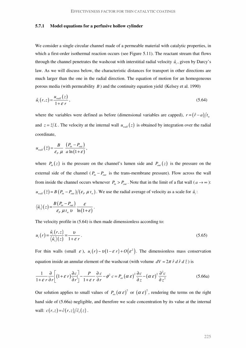
EFFECTIVENESS FACTOR FOR THIN CATALYTIC COATINGS
225
5.7.1 Model equations for a perfusive hollow cylinder
We consider a single circular channel made of a permeable material with catalytic properties, in
which a first-order isothermal reaction occurs (see Figure 5.11). The reactant stream that flows
through the channel penetrates the washcoat with interstitial radial velocity ˆi
u , given by Darcy’s
law. As we will discuss below, the characteristic distances for transport in other directions are
much larger than the one in the radial direction. The equation of motion for an homogeneous
porous media (with permeability B ) and the continuity equation yield (Kelsey et al. 1990)
( )( )
ˆ ,1
wall
i
u zu r z
rε=
+, (5.64)
where the variables were defined as before (dimensional variables are capped), ( )ˆw
r r a t= −
and ˆz z L= . The velocity at the internal wall ( )wallu z is obtained by integration over the radial
coordinate,
( )( )
( )ˆ
ln 1in out
wall
P
P PBu z
aε µ ε
−=
+,
where ( )inP z is the pressure on the channel’s lumen side and ( )out
P z is the pressure on the
external side of the channel (in out
P P− is the trans-membrane pressure). Flow across the wall
from inside the channel occurs whenever in out
P P> . Note that in the limit of a flat wall ( a → ∞ ):
( ) ( ) ( )ˆwall in out P w
u z B P P tε µ= − . We use the radial average of velocity as a scale for ˆi
u :
( )( )
( )ˆ
ln 1in out
i
P w
B P Pu z
t
ε
ε µ υ ε
−=
+.
The velocity profile in (5.64) is then made dimensionless according to:
( )( )
( )
ˆ ,
ˆ 1i
i
i
u r zu r
u z r
υ
ε= =
+. (5.65)
For thin walls (small ε ), ( ) ( ) ( )2~ 1
iu r r Oυ ε ε− + . The dimensionless mass conservation
equation inside an annular element of the washcoat (with volume ˆ ˆ ˆ2dV r d r d zπ= ) is
( ) ( ) ( )
22 22
2
11
1 1 ax
c P c c cr c P
r r r r r z zε φ α ε α ε
ε ε
∂ ∂ ∂ ∂ ∂+ − − = −
+ ∂ ∂ + ∂ ∂ ∂ (5.66a)
Our solution applies to small values of ( )2
axP α ε or ( )
2α ε , rendering the terms on the right
hand side of (5.66a) negligible, and therefore we scale concentration by its value at the internal
wall: ( ) ( ) ( )1ˆ ˆ, ,c r z c r z c z= .

CHAPTER 5
226
Figure 5.11: Perfusive monolith with wall thickness w
t and radius of the circular open channel
a . Intraparticular flow direction is represented for in out
P P> with velocity profile ˆi
u .
Surface concentrations are 1c and 2c .
For simplicity , we solve the problem for the case of specified concentration at both surfaces of
the channel:
1c = at 0r = (5.66b)
( )2c c z= at 1r = . (5.66c)
These surface concentrations are determined when solving the internal and external convection-
diffusion problems. The parameters (and/or functions of the axial variable) appearing in
Eqs.(5.66) are:
Intraparticular radial Peclet number: ( )
( )
ˆ
ln 1P i w in out
eff eff
u t B P PP
D D
ε υ ε
µ ε
−= =
+ (5.67a)
Intraparticular axial Peclet number: P ax
ax
ax
u LP
D
ε= (5.67b)
Thiele modulus: 2
2 w
eff
t k
Dφ = (5.67c)
Washcoat-channel length scales ratio: wt
aε = (5.67d)
Aspect ratio: ax
eff
Da
L Dα = (5.67e)
Ratio of surface concentration distributions: 22
1
ˆ
ˆc
cc
= (5.67f)
wt a
r
z
( )ˆ ˆ ˆ,i
u r z
( )1 ˆc z( )2ˆ ˆc z ( )ˆin
P z ( )ˆout
P z

EFFECTIVENESS FACTOR FOR THIN CATALYTIC COATINGS
227
When neglecting axial diffusion and convection, besides typical geometrical features (w
t L<< ),
we have assumed that the permeability in this direction may be much smaller than the one in the
radial direction. The axial dependence of the solution is thus given by the parameters and
boundary conditions.
The radially averaged effectiveness factor (referred to internal surface conditions) is
( ) ( ) ( )
1
22 20 1 0
1 11 1 1
r r
c c Pr c dr c
r rη ε ε
υ φ υ φ υ= =
∂ ∂= + = + − + −
∂ ∂ ∫ . (5.68)
5.7.2 Perturbation solution for specified surface concentration and pressure profiles
A simplified solution is obtained below for the following parameter magnitude relationship:
( ) ( )2 2, 1
axPα ε α ε ε<< << . There is no need to restrict the magnitude of 2
φ , P and 2c , since
the kinetic law is linear and an analytical solution is possible without further simplification. We
take ε as a small parameter and look for a perturbation expansion for the concentration profile
of the following form:
( ) ( ) ( ) ( )2
0 1c r c r c r Oε ε= + + . (5.69)
The first two subproblems extracted from Eqs.(5.66) give the solution to the coefficients ( )0c r
and ( )1c r :
( )0
O ε : ( )
220 0
020
c cP c
r rε φ
∂ ∂− − − =
∂ ∂ (5.70a)
( )0 0 1c r = = (5.70b)
( )0 21c r c= = (5.70c)
( )1
O ε : ( ) ( )
22 01 1
12
cc cP c P r
r r rε φ ε
∂∂ ∂− − − = − −
∂ ∂ ∂ (5.71a)
( )1 0 0c r = = (5.71b)
( )1 1 0c r = = (5.71c)
A convenient redefinition of Peclet number with curvature effects is suggested by Eqs. (5.70a)
and (5.71a): C
P P ε= − . The corresponding perturbation series for the effectiveness factor is
( )2
0 1 Oη η ε η ε= + + . (5.72a)

CHAPTER 5
228
Table 5.3: Maximum relative error between ( )2
η φ calculated numerically (gPROMS®) and
from Eq.(5.73) with 2 1c = . The numbers in brackets correspond to the value of
Thiele modulus where the maximum is observed.
CP
ε 0.1 1 5 10 100
0.1 0.0004%
(16)
0.003%
(15)
0.007%
(28)
0.02%
(67)
0.06%
(136)
0.5 0.006%
(12)
0.04%
(11)
0.13%
(31)
0.39%
(67)
1.18%
(128)
1 0.02%
(12)
0.11%
(11)
0.32%
(31)
1.06%
(64)
3.8%
(122)
Figure 5.12: Effectiveness factor plot ( )2
η φ in a hollow perfusive cylinder with 0.1ε = and
for several values of the intraparticular Peclet number. Full lines are the result of
numerical simulation. Dashed lines represent the approximate solution (5.73).
0.1
0.2
0.3
0.4
0.5
0.6
0.7
0.8
0.9
1
0.01 0.1 1 10 100
numerical
perturbation
η
2φ
1P =
5P =
10P =
50P =0.1ε =
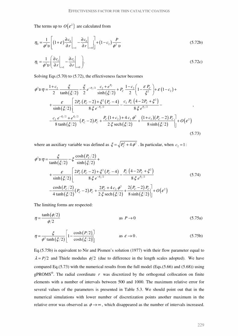
EFFECTIVENESS FACTOR FOR THIN CATALYTIC COATINGS
229
The terms up to ( )2
O ε are calculated from
( ) ( )0 0
0 22 2
1 0
11 1
r r
c c Pc
r rη ε
φ υ φ υ= =
∂ ∂= + − + −
∂ ∂ (5.72b)
1 11 2
1 0
1
r r
c c
r rη
φ υ= =
∂ ∂= − ∂ ∂
. (5.72c)
Solving Eqs.(5.70) to (5.72), the effectiveness factor becomes
( ) ( )( )
( )
( ) ( ) ( )
( )( )
( )
( )
( )( )
( )( )
22 2 2 222
222
2 2
22 22 2 2 22
1 11 1
2 tanh 2 2 sinh 2 2
4 22 2 4
sinh 2 8 8
1 4 1 22
8 tanh 2 2 sech 2 8 sinh 2
C
C
C C
C C
P
P C
C
C CC C C
P P
P P
C C C
C C
Pc c e ce P c
c P PP P P
e e
P c c c P Pc e eP P O
εξ ξφ υ η ε
ξ ξ ξ
ξξε
ξ ξ ξ
φε
ξ ξ ξ ξ
−
−
−
+ + −= − + − + − +
− +− + −+ − −
+ + + −+− − + + +
,
(5.73)
where an auxiliary variable was defined as 2 24C
Pξ φ= + . In particular, when 2 1c = :
( )
( )
( )
( )
( ) ( ) ( )
( )
( )( )
( )
( )
( )( )
2
22
2 2
222
cosh 2
tanh 2 sinh 2
4 22 2 4
sinh 2 8 8
cosh 2 2 22 42
4 tanh 2 2 sech 2 8 sinh 2
C C
C
C CC C C
P P
C C CC
C C
P
P PP P P
e e
P P PP cP P O
ξφ υ η ξ
ξ ξ
ξξε
ξ ξ ξ
φε
ξ ξ ξ ξ
−
= − +
− +− + −+ −
−+− − + + +
(5.74)
The limiting forms are respected:
( )tanh 2
2
φη
φ= as 0P → (5.75a)
( )
( )
( )2
cosh 21
tanh 2 cosh 2
Pξη
φ ξ ξ
= −
as 0ε → . (5.75b)
Eq.(5.75b) is equivalent to Nir and Pismen’s solution (1977) with their flow parameter equal to
2Pλ = and Thiele modulus 2φ (due to difference in the length scales adopted). We have
compared Eq.(5.73) with the numerical results from the full model (Eqs.(5.66) and (5.68)) using
gPROMS®. The radial coordinate r was discretized by the orthogonal collocation on finite
elements with a number of intervals between 500 and 1000. The maximum relative error for
several values of the parameters is presented in Table 5.3. We should point out that in the
numerical simulations with lower number of discretization points another maximum in the
relative error was observed as φ → ∞ , which disappeared as the number of intervals increased.

CHAPTER 5
230
Therefore, Eq.(5.73) also avoids the numerical convergence issues in the diffusional controlled
limit. The effectiveness factor curves ( )2
η φ are plotted in Figure 5.12. For other values of 2c ,
the agreement between numerical and analytical solutions is comparable to this case.
It is important to note the good agreement observed even for reasonably high values of ε (note
that our solution was conceived for small values of ε ). At leading-order, the convection,
diffusion and reaction problem in a slab catalyst is recovered, for which analytical solutions
have been presented for a number of cases (e.g. zero-order kinetics (Rodrigues et al. 1984),
consecutive-parallel reactions (Nir 1977; Cresswell 1985) and nonisothermal behavior (Cardoso
et al. 2007), also discussed in Chapter 6 of this thesis). In certain limits, a curvature correction
for these situations may also be obtained and added as a ( )O ε term.
Figure 5.13: Concentration profile in the convection dominated regime for 3 values of the
surface concentration at the outer surface of the cylinder. Comparison between
perturbation composite solution (5.79) (dashed lines) and numerical solution (full lines).
Parameters: 50C
P = , 2 50φ = , 0.1ε = and ( )1 0.35out
c r = = .
0
1
2
3
4
0
0.1
0.2
0.3
0.4
0.5
0.6
0.7
0.8
0.9
1
0 0.1 0.2 0.3 0.4 0.5 0.6 0.7 0.8 0.9 1
numerical
perturbation
( )c r
r
( )2 1out
c c r= =
( )2 10 1out
c c r= =
( )2 0.1 1out
c c r= =
( )c r

EFFECTIVENESS FACTOR FOR THIN CATALYTIC COATINGS
231
5.7.3 Performance enhancement
It is well-known (Nir et al. 1977; Rodrigues 1981; Rodrigues et al. 1991) that the effect of an
additional mass transport mechanism is to increase the overall content of the pellet in reactant
species, and therefore an increase in the effectiveness factor may be observed. The enhancement
due to the intraparticular flow can be quantified by
( )
( )
2
2
,
, 0
P
P
η φ
η φΕ =
=. (5.76)
There is a maximum in the ( )2
φΕ curves with respect to the parameter 2φ , which increases as
P increases (Figure 5.14). When 1P >> , the internal mass transport is dominated by
convection, but for the effect to be visible in the observed reaction rate, kinetics should also be
reasonable fast (otherwise no enhancement would be observed), so 2 1φ >> (see Figure 5.14).
The conditions under which maximum advantage is taken from the catalyst’s permeability are
detailed below. It is important to characterize this regime, since in others the enhancement is
less pronounced. An approximate solution to the concentration profile can be built using the
boundary layer method (Bender et al. 1978). For convection-dominated operation (diffusional
limitation in the transport), the outer domain ( 0 1r δ≤ < − ) is described by
210
1out
out
C
cc
r r P
φ
ε
∂+ =
+ ∂ ( 1P >> , 2~P φ ) (5.77a)
( )0 1out
c r = = , (5.77b)
where it is assumed that the direction of the flow is from the lumen towards the exterior. The
boundary condition at 1r = only happens to be fulfilled by (5.77) if
( )
2
21 exp 12out
C
c r cP
φ ε = = − + =
which does not happen in general. Therefore, a boundary layer exists at the external surface
(from where flow exits the monolith). An appropriate description for this region (1 1rδ− < ≤ )
includes a convective-diffusive balance given by
2
20in in
c c
R R
∂ ∂+ =
∂ ∂ (5.78a)
( ) 20in
c R c= = , (5.78b)
with ( )1C
R P r= − . Both solutions match in an intermediate domain ( ( ) ( )1out in
c r c R→ = → ∞ )
to yield the following composite solution:

CHAPTER 5
232
Figure 5.14: Enhancement curves ( )2
φΕ of the effectiveness factor in a hollow cylinder due
to internal radial convection. Both surfaces are maintained at the same concentration
and results for several values of P and ε are shown. The approximate relationship for
the maximum effectiveness factor maxΕ in Eq.(5.82) is shown as a thick dashed line.
Figure 5.15: Effect of asymmetry in the boundary conditions on the enhancement curves
( )2
φΕ . The concentration ratio is 2 0.1c = and results for several values of P and
0.1ε = are shown. maxΕ from Eq.(5.82) is shown as a thick dashed line.
1
1.2
1.4
1.6
1.8
2
2.2
2.4
0.1 1 10 100 1000
1ε =
0.1ε =
50P =
10P =
1P =
2φ
Ε
maxΕ
1.0
1.5
2.0
2.5
3.0
3.5
4.0
4.5
0.1 1 10 100 1000
50P =
10P =
2φ
Ε maxΕ

EFFECTIVENESS FACTOR FOR THIN CATALYTIC COATINGS
233
( )( )
( )
2 2
1 112 2 1
2CC C
rr
P rP P
Cc r e c e e O P
φ ε φ ε− − + +
− − − = + − +
with ( )
2
~ 1C
OP
φ. (5.79)
This solution is plotted in Figure 5.13 for 50P = , 2 50φ = and 0.1ε = . For this case,
( )1 0.35out
c r = = , and we choose three concentration profiles with: ( )2 1out
c c r= = ,
( )2 10 1out
c c r= = and ( )2 0.1 1out
c c r= = . The presence of boundary layers near 1r = for the
two latter cases is well described by the composite solution.
The corresponding effectiveness factor is according to Eq.(5.68):
( )( )
( )
2 2 2
2222
1 1 1~ 1 1 1 1
C
C C C C
PCP P P PC
C C
c PPe e c e e
P P
φ υ φ υ φ υ
η ε ε ευ φ υ
− −− −
−
+ − − + + − + + − +
.
(5.80)
A simple estimate of the enhancement factor defined in (5.76) can be obtained in the limit of
small ε and high C
P ,
( ) ( )
2
222
~ 11 tanh 2
CPCP
e cc
φ υ
φε
υ φ φ
− Ε − +
+
The maximum of Ε with respect to φ is calculated from (for reasonably high φ but 2 ~ 1Pφ ),
( )
2 22
1 2C CP P
C
e e OP
φ υ φ υ
φ υε
− −
− = +
and therefore, the optimum set of parameters ( 2C
Pφ υ ) is approximately described by a
constant ratio of the timescales for convection and reaction, with the following numerical value:
2
1.2564opt
CP
υ φ= ( 1P >> and 1ε << ). (5.81)
Eq.(5.81) gives a conservative estimate for C
P , which improves as 1P >> . This corresponds to
a maximum enhancement of
( ) ( )max
2
0.5694
1 tanh 2opt
optc
φ
φΕ =
+. (5.82)
Eqs.(5.81) and (5.82) give an approximate loci of the maxima points on the enhancement factor
curves. These are plotted in Figure 5.14 for the symmetric case and in Figure 5.15 for the
asymmetric case. In the latter case ( 2 1c < ), the enhancement in the chemical regime is greater
than 1, since the convective flow increases concentration significantly in comparison to the
linear profile predicted by diffusion alone. In this case, the reactant is being transferred from the
outer surface ( 1r = ) into the bulk, yielding ( ) ( )20 1 2 1cη φ → = + < . This limit corresponds to:

CHAPTER 5
234
( ) 2
2
120 1
1C
c
c Pφ
−Ε → = +
+ for 1
CP >> .
Therefore, when a concentration difference exists the improvement brought by convection can
be very significant. For moderate values of C
P , the estimates from (5.81) and (5.82) can still be
useful. For a specified value of Thiele modulus, (5.81) overestimates the intraparticular Peclet
number at which maximum enhancement is observed (given correctly by (5.82)). For a specified
intraparticular Peclet number, opt
φ is underestimated. In both cases, a lower bound for the
maximum enhancement is obtained from (5.82), while the actual improvement can be slightly
larger. These differences become negligible in the convection dominated limit ( 1C
P >> ). Also,
the result from (5.81) is quite insensitive to the values of 2c (associated with ε ).
5.8 CONCLUSIONS
We have addressed several questions related with the internal transport-reaction problem in a
catalytic coating, using the classical effectiveness factor concept. First, we focused on the issue
of the evaluation of the effectiveness factor itself and proposed an approximate calculation
procedure with the following characteristics:
(a) A very simple expression based on a typical geometrical characteristic found in wall-coated
microreactors was derived, and is valid for all values of Thiele modulus. This compares
very favorably with methods presented in current literature where more complex shape
factors are obtained for low and high 2φ , resulting sometimes in a fragmented analysis.
(b) For some classes of nonlinear kinetics, our solution fulfills the asymptotic behavior at small
and large reaction rates, and presents small errors in the intermediate range. For this case,
we presented a generalization of the Thiele modulus which includes the classical
normalizations in their ranges of validity.
(c) An arbitrary geometry is described by our solution by a measurable shape parameter (which
combines the washcoat volume, surface area and thickness) and by the effectiveness factor
of an equivalent slab.
(d) The performance of the ‘slice method’ (Papadias et al. 2000b) is improved, without
introducing further complexity. This involved the consideration of a curvature correction,
which reduced the relative error or the number of slices required to achieve a satisfactory
approximation, especially in the intermediate regime of Thiele modulus.

EFFECTIVENESS FACTOR FOR THIN CATALYTIC COATINGS
235
(e) Despite the fact that our analysis was built for thin coatings, in some cases acceptable
results were obtained even for ~ 1ε . Also, even though our main focus was on
microchannel reactors, egg-shell catalyst particles and hollow cylinders can also benefit
from our approach.
The second part of our work was concerned with the definition of operating regimes in wall-
coated microchannels. We have extended previous analyses (Chapter 4) to consider the
interplay between internal and external controlling processes. We have shown that, even though
channel and washcoat domains are coupled, the solution of the full model is not required for
estimation of boundaries between regimes. Even if variation of all properties with temperature
needs to be accounted for, the problem can be reduced to the solution of a set of nonlinear
algebraic equations. We predict that the process which determines the limiting behavior is
governed by the ratio of ‘diffusion velocity’ in the washcoat and in the channel ( ( )effD Dε ).
This has implications in experimental and modeling methods for measurement of intrinsic
kinetics (requiring chemically controlled conditions) and operation in the mass transfer
controlled limit. Current studies have neglected the role of this parameter and contradictory
conclusions regarding the presence/absence of mass transfer limitations can be explained by
taking it into consideration. Regime maps are presented with the parametric regions where
channel and coating can be considered to operate under chemical and diffusional control
(independently or together).
Finally, performance enhancement of a catalytic coating by intraparticular convection is
explored. An approximation to the effectiveness factor in the case of radial convective flow is
presented for a hollow cylinder and gives very acceptable results for a wide range of the
parameters (including the ratio of surface concentrations at the inner and outer walls). We have
also looked at the conditions under which the enhancement due to internal convection was more
pronounced. The original work of Nir and Pismen (1977) identify these conditions as the ones
where “the kinetics just becomes diffusion controlled”. In their analysis this happened for
Thiele modulus of order 1. However, considering a regime with fast convective transport, but
where reaction is also fast enough, we have observed an optimum range of operation and
design. When the rate of reactant consumption is able to keep up with strong convection, the
pellet should be designed so that the (short) timescale for convection is approximately 1.26
times higher than the one for reaction. The observed enhancement is proportional to the square
root of the intraparticular Peclet number:
max2
0.6382
1C
P
c υΕ =
+.

CHAPTER 5
236
NOTATION
a characteristic distance for diffusion in the channel
A cross-sectional area of washcoat
B permeability of the medium
mBi mass Biot number
c dimensionless concentration of reactant in the washcoat
2c ratio between concentrations at the surfaces
C concentration of reactant in the channel
D diffusivity in the bulk
axD effective diffusivity in the coating (axial)
effD effective diffusivity in the coating (transverse)
Da Damköhler number
E activation energy
Ε enhancement factor
2 1F hypergeometric function
0k pre-exponential factor in reaction kinetics
K kinetic parameter
L length of the channel
LHS left hand side
m order of reaction
p kinetic parameter
P intraparticular Peclet number
P∇ pressure gradient vector
r dimensionless transverse coordinate
R reaction rate
RHS right hand side
GR ideal gas constant
S area of the channel-coating interface
Sh Sherwood number
wt thickness of the catalytic coating
T temperature
ˆi
u interstitial (pore) velocity
V washcoat volume
iw fraction of the washcoat volume correspondent to a slice
z dimensionless axial coordinate

EFFECTIVENESS FACTOR FOR THIN CATALYTIC COATINGS
237
Greek letters
α aspect ratio of the channel
mPe
z
α Graetz parameter
ε ratio of the characteristic distances for diffusion in the coating and in the channel
Pε porosity of catalytic coating or membrane
φ Thiele modulus
µ dynamic viscosity
η effectiveness factor
η global effectiveness factor
σ shape parameter
τ timescale
θ degree of mass transfer control; angular coordinate
υ volume to surface ratio, divided by characteristic dimension for diffusion
Superscripts
^ dimensional quantities
‘ normalized by inlet conditions
Subscripts
in referred to inlet conditions
surf referred to surface conditions
transv transverse
V per volume of washcoat
REFERENCES
Afeyan, N. B., S. P. Fulton, N. F. Gordon, I. Mazsaroff, L. Varady and F. E. Regnier (1990a). "Perfusion chromatography: An approach to purifying biomolecules." Nature Biotechnology 8(3): 203-206.
Afeyan, N. B., S. P. Fulton and F. E. Regnier (1991). "Perfusion chromatography packing materials for proteins and peptides." Journal of Chromatography 544(1-2): 267-279.
Afeyan, N. B., N. F. Gordon, I. Mazsaroff, L. Varady, S. P. Fulton, Y. B. Yang and F. E. Regnier (1990b). "Flow-through particles for the high-performance liquid chromatographic separation of biomolecules: Perfusion chromatography." Journal of Chromatography 519(1): 1-29.
Aran, H. C., J. K. Chinthaginjala, R. Groote, T. Roelofs, L. Lefferts, M. Wessling and R. G. H. Lammertink (2011). "Porous ceramic mesoreactors: A new approach for gas-liquid contacting in multiphase microreaction technology." Chemical Engineering Journal 169(1-3): 239-246.
CHAPTER 5
238
Aris, R. (1975). The mathematical theory of diffusion and reaction in permeable catalysts. London, Oxford University Press.
Bakker, J. J. W., W. J. Groendijk, K. M. De Lathouder, F. Kapteijn, J. A. Moulijn, M. T. Kreutzer and S. A. Wallin (2007). "Enhancement of catalyst performance using pressure pulses on macroporous structured catalysts." Industrial and Engineering Chemistry Research 46(25): 8574-8583.
Bakker, J. J. W., M. T. Kreutzer, K. De Lathouder, F. Kapteijn, J. A. Moulijn and S. A. Wallin (2005). "Hydrodynamic properties of a novel 'open wall' monolith reactor." Catalysis Today 105(3-4): 385-390.
Bender, C. M. and S. A. Orszag (1978). Advanced Mathematical Methods for Scientists and Engineers. New York, McGraw-Hill.
Bischoff, K. B. (1967). "An extension of the general criterion for importance of pore diffusion with chemical reactions." Chemical Engineering Science 22(4): 525-530.
Bouzek, K. and I. Roušar (1996). "Comparison of the effectiveness factors for a reaction at a pore wall calculated on the assumption of the Langmuir-Hinshelwood mechanism and according to a power equation." Journal of Chemical Technology and Biotechnology 66(2): 131-134.
Burghardt, A. and A. Kubaczka (1996). "Generalization of the effectiveness factor for any shape of a catalyst pellet." Chemical Engineering and Processing: Process Intensification 35(1): 65-74.
Cardoso, S. S. S. and A. E. Rodrigues (2007). "Convection, diffusion and reaction in a nonisothermal, porous catalyst slab." AIChE Journal 53(5): 1325-1336.
Cedro III, V. and S. Srinivasan (1974). "Heat and mass transfer in a porous wall tubular reactor." International Journal of Heat and Mass Transfer 17(11): 1413-1416.
Chen, G. and A. F. Palmer (2009). "Hemoglobin-based oxygen carrier and convection enhanced oxygen transport in a hollow fiber bioreactor." Biotechnology and Bioengineering 102(6): 1603-1612.
Chen, X. B., Y. Sui, Y. P. Cheng, H. P. Lee, P. Yu, S. H. Winoto and H. T. Low (2010a). "Mass transport in a microchannel enzyme reactor with a porous wall: Hydrodynamic modeling and applications." Biochemical Engineering Journal 52(2-3): 227-235.
Chen, X. B., Y. Sui, H. P. Lee, H. X. Bai, P. Yu, S. H. Winoto and H. T. Low (2010b). "Mass transport in a microchannel bioreactor with a porous wall." Journal of Biomechanical Engineering 132(6).
Chou, C. T. and W. E. Stewart (1986). "Influence of coating geometry on the effectiveness of monolithic catalysts." Chemical Engineering Science 41(1): 202-204.
CIM Convective Interaction Media(R) . Liquid Chromatography RedesignedTM. www.monoliths.com. BIASeparations.
Coletti, F., S. Macchietto and N. Elvassore (2006). "Mathematical modeling of three-dimensional cell cultures in perfusion bioreactors." Industrial and Engineering Chemistry Research 45(24): 8158-8169.
Cresswell, D. L. (1985). "Intra-particle convection: its measurement and effect on catalyst activity and selectivity." Applied catalysis 15(1): 103-116.
Datta, R. and S. W. K. Leung (1985). "Shape generalized isothermal effectiveness factor for first-order kinetics." Chemical Engineering Communications 39(1): 155 - 173.

EFFECTIVENESS FACTOR FOR THIN CATALYTIC COATINGS
239
De Lathouder, K. M., J. Bakker, M. T. Kreutzer, F. Kapteijn, J. A. Moulijn and S. A. Wallin (2004). "Structured reactors for enzyme immobilization: Advantages of tuning the wall morphology." Chemical Engineering Science 59(22-23): 5027-5033.
Froment, G. F. and K. B. Bischoff (1979). Chemical Reactor Analysis and Design New York, Wiley.
Gavriilidis, A. and A. Varma (1992). "Optimal catalyst activity profiles in pellets: 9. Study of ethylene epoxidation." AIChE Journal 38(2): 291-296.
Germani, G. and Y. Schuurman (2006). "Water-gas shift reaction kinetics over micro-structured Pt/CeO2/AI2O3 catalysts." AIChE Journal 52(5): 1806-1813.
Gonzo, E. E. (2008). "Hydrogen from methanol-steam reforming. Isothermal and adiabatic monolith reactors' simulation." International Journal of Hydrogen Energy 33(13): 3511-3516.
Gonzo, E. E. and J. C. Gottifredi (2011). "Heat and mass transfer limitations in monolith reactor simulation with non uniform washcoat thickness." Latin American Applied Research 40(1): 15-21.
Görke, O., P. Pfeifer and K. Schubert (2009). "Kinetic study of ethanol reforming in a microreactor." Applied Catalysis A: General 360(2): 232-241.
Gottifredi, J. C. and E. E. Gonzo (1986). Application of perturbation and matching techniques to solve transport phenomena problems. Advances in Transport Processes. A. Mujumdar and R. A. Mashelkar. New Delhi, Wiley Eastern. IV: 419-464.
Gottifredi, J. C. and E. E. Gonzo (2005a). "Approximate expression for the effectiveness factor estimation and a simple numerical method for concentration profile calculation in porous catalyst." Chemical Engineering Journal 109(1): 83-87.
Gottifredi, J. C. and E. E. Gonzo (2005b). "On the effectiveness factor calculation for a reaction - Diffusion process in an immobilized biocatalyst pellet." Biochemical Engineering Journal 24(3): 235-242.
Gottifredi, J. C., E. E. Gonzo and O. D. Quiroga (1981). "Isothermal effectiveness factor-I. Analytical expression for single reaction with arbitrary kinetics. Slab geometry." Chemical Engineering Science 36(4): 713-719.
Groppi, G., W. Ibashi, M. Valentini and P. Forzatti (2001). "High-temperature combustion of CH4 over PdO/Al2O3: Kinetic measurements in a structured annular reactor." Chemical Engineering Science 56(3): 831-839.
Hayes, R. E. and S. T. Kolaczkowski (1994). "Mass and heat transfer effects in catalytic monolith reactors." Chemical Engineering Science 49(21): 3587-3599.
Hayes, R. E., B. Liu, R. Moxom and M. Votsmeier (2004). "The effect of washcoat geometry on mass transfer in monolith reactors." Chemical Engineering Science 59(15): 3169-3181.
Hayes, R. E., B. Liu and M. Votsmeier (2005). "Calculating effectiveness factors in non-uniform washcoat shapes." Chemical Engineering Science 60(7): 2037-2050.
Haynes Jr, H. W. (1986). "An explicit approximation for the effectiveness factor in porous heterogeneous catalysts." Chemical Engineering Science 41(2): 412-415.
Horvath, C. and J. M. Engasser (1973). "Pellicular heterogeneous catalysts. A theoretical study of the advantages of shell structured immobilized enzyme particles." Industrial and Engineering Chemistry 12(2): 229-235.

CHAPTER 5
240
Jensen, K. F. (2001). "Microreaction engineering-is small better?" Chemical Engineering Science 56(2): 293-303.
Joshi, S. Y., M. P. Harold and V. Balakotaiah (2010). "Overall mass transfer coefficients and controlling regimes in catalytic monoliths." Chemical Engineering Science 65(5): 1729-1747.
Joshi, S. Y., Y. Ren, M. P. Harold and V. Balakotaiah (2011). "Determination of kinetics and controlling regimes for H2 oxidation on Pt/Al2O3 monolithic catalyst using high space velocity experiments." Applied Catalysis B: Environmental 102(3-4): 484-495.
Kalluri, R. R., D. R. Cahela and B. J. Tatarchuk (2009). "Comparative heterogeneous contacting efficiency in fixed bed reactors: Opportunities for new microstructured systems." Applied Catalysis B: Environmental 90(3-4): 507-515.
Kapteijn, F., R. M. De Deugd and J. A. Moulijn (2005). "Fischer-Tropsch synthesis using monolithic catalysts." Catalysis Today 105(3-4): 350-356.
Kapteijn, F., T. A. Nijhuis, J. J. Heiszwolf and J. A. Moulijn (2001). "New non-traditional multiphase catalytic reactors based on monolithic structures." Catalysis Today 66(2-4): 133-144.
Keegan, S. D., N. J. Mariani, S. P. Bressa, G. D. Mazza and G. F. Barreto (2003). "Approximation of the effectiveness factor in catalytic pellets." Chemical Engineering Journal 94(2): 107-112.
Keegan, S. D., N. J. Mariani, O. M. Martínez and G. F. Barreto (2005). "Behaviour of smooth catalysts at high reaction rates." Chemical Engineering Journal 110(1-3): 41-56.
Kelsey, L. J., M. R. Pillarella and A. L. Zydney (1990). "Theoretical analysis of convective flow profiels in a hollow-fiber membrane bioreactor." Chemical Engineering Science 45(11): 3211-3220.
Khassin, A. A., A. G. Sipatrov, G. K. Chermashetseva, T. M. Yurieva and V. N. Parmon (2005a). "Fischer-Tropsch synthesis using plug-through contactor membranes based on permeable composite monoliths. Selectivity control by porous structure parameters and membrane geometry." Topics in Catalysis 32(1-2): 39-46.
Khassin, A. A., A. G. Sipatrov, T. M. Yurieva, G. K. Chermashentseva, N. A. Rudina and V. N. Parmon (2005b). "Performance of a catalytic membrane reactor for the Fischer-Tropsch synthesis." Catalysis Today 105(3-4): 362-366.
Khassin, A. A., T. M. Yurieva, A. G. Sipatrov, V. A. Kirillov, G. K. Chermashentseva and V. N. Parmon (2003). "Fischer-Tropsch synthesis using a porous catalyst packing: Experimental evidence of an efficient use of permeable composite monoliths as a novel type of the Fischer-Tropsch synthesis catalyst." Catalysis Today 79-80: 465-470.
Kiwi-Minsker, L. and A. Renken (2005). "Microstructured reactors for catalytic reactions." Catalysis Today 110(1-2): 2-14.
Kolb, G., V. Hessel, V. Cominos, C. Hofmann, H. Löwe, G. Nikolaidis, R. Zapf, A. Ziogas, E. R. Delsman, M. H. J. M. de Croon, J. C. Schouten, O. de la Iglesia, R. Mallada and J. Santamaria (2007). "Selective oxidations in micro-structured catalytic reactors--For gas-phase reactions and specifically for fuel processing for fuel cells." Catalysis Today 120(1): 2-20.
Kreutzer, M. T., F. Kapteijn and J. A. Moulijn (2006). "Shouldn't catalysts shape up? Structured reactors in general and gas-liquid monolith reactors in particular." Catalysis Today 111(1-2): 111-118.
Lee, J. and D. H. Kim (2006). "An approximation method for the effectiveness factor in porous catalysts." Chemical Engineering Science 61(15): 5127-5136.
EFFECTIVENESS FACTOR FOR THIN CATALYTIC COATINGS
241
Lee, W.-C., G.-J. Tsai and G. T. Tsao (1990). Radial-Flow Affinity Chromatography for Trypsin Purification. Protein Purification: From Molecular Mechanisms to Large-Scale Processes. M. R. Ladisch, R. C. Willson, C. C. Painton and S. E. Builder, American Chemical Society: 104-117.
Leung, D., R. E. Hayes and S. T. Kolaczkowskl (1996). "Diffusion Limitation Effects in the Washcoat of a Catalytic Monolith Reactor." Canadian Journal of Chemical Engineering 74(1): 94-103.
Lewis, W. and S. Middleman (1974). "Conversion in a hollow fiber membrane / enzyme reactor." AIChE Journal 20(5): 1012-1014.
Lu, Z. P., M. M. Dias, J. C. B. Lopes, G. Carta and A. E. Rodrigues (1993). "Diffusion, convection, and reaction in catalyst particles: Analogy between slab and sphere geometries." Industrial and Engineering Chemistry Research 32(9): 1839-1852.
Magyari, E. (2008). "Exact analytical solution of a nonlinear reaction-diffusion model in porous catalysts." Chemical Engineering Journal 143(1-3): 167-171.
Mariani, N. J., S. D. Keegan, O. M. Martínez and G. F. Barreto (2003). "A one-dimensional equivalent model to evaluate overall reaction rates in catalytic pellets." Chemical Engineering Research and Design 81(8): 1033-1042.
Mariani, N. J., S. D. Keegan, O. M. Martínez and G. F. Barreto (2008a). "On the evaluation of effective reaction rates on commercial catalyst by means of a one-dimensional model." Catalysis Today 133-135(1-4): 770-774.
Mariani, N. J., S. D. Keegan, O. M. Martínez and G. F. Barreto (2008b). "On the evaluation of effective reaction rates on commercial catalyst by means of a one-dimensional model." Catalysis Today 133-135(1-4): 770-774.
Mariani, N. J., C. Mocciaro, S. D. Keegan, O. M. Martínez and G. F. Barreto (2009a). "Evaluating the effectiveness factor from a 1D approximation fitted at high Thiele modulus: Spanning commercial pellet shapes with linear kinetics." Chemical Engineering Science 64(11): 2762-2766.
Mariani, N. J., C. Mocciaro, O. M. Martínez and G. F. Barreto (2009b). "Estimation of effectiveness factor for arbitrary particle shape and non-linear kinetics." Industrial and Engineering Chemistry Research 48(3): 1172-1177.
Mocciaro, C., N. J. Mariani, O. M. Martínez and G. F. Barreto (2011). "A three-parameter one-dimensional model to predict the effectiveness factor for an arbitrary pellet shape." Industrial and Engineering Chemistry Research 50(5): 2746-2754.
Mogalicherla, A. K. and D. Kunzru (2010). "Effect of gas and liquid superficial velocities on the performance of monolithic reactors." Industrial and Engineering Chemistry Research 49(4): 1631-1641.
Motamedhashemi, M. M. Y., F. Egolfopoulos and T. Tsotsis (2011). "Application of a Flow-Through Catalytic Membrane Reactor (FTCMR) for the Destruction of a Chemical Warfare Simulant." Journal of Membrane Science In Press, Accepted Manuscript.
Nagy, E. (2010a). "Convective and diffusive mass transport through anisotropic, capillary membrane." Chemical Engineering and Processing: Process Intensification 49(7): 716-721.
Nagy, E. (2010b). "Mass transfer through a convection flow catalytic membrane layer with dispersed nanometer-sized catalyst." Industrial and Engineering Chemistry Research 49(3): 1057-1062.
Nan, H. S., M. M. Dias, J. C. B. Lopes and A. E. Rodrigues (1996a). "Diffusion, convection and reaction in catalyst particles: Analogy between slab and cylinder geometries." Chemical Engineering Journal and the Biochemical Engineering Journal 61(2): 113-122.

CHAPTER 5
242
Nan, H. S., M. M. Dias, V. G. Mata and A. E. Rodrigues (1996b). "Measurements of effective diffusivity in large-pore permeable pellets with various geometries using the chromatographic method." Chemical Engineering Communications 146: 201-229.
Nir, A. (1977). "Simultaneous intraparticle forced convection, diffusion and reaction in a porous catalyst - 2. Selectivity of sequential reactions." Chemical Engineering Science 32(8): 925-930.
Nir, A. and L. M. Pismen (1977). "Simultaneous intraparticle forced convection, diffusion and reaction in a porous catalyst." Chemical Engineering Science 32(1): 35-41.
Ouyang, X., L. Bednarova, R. S. Besser and P. Ho (2005). "Preferential oxidation (PrOx) in a thin-film catalytic microreactor: Advantages and limitations." AIChE Journal 51(6): 1758-1772.
Papadias, D., L. Edsberg and P. Björnbom (2000a). "Simplified method of effectiveness factor calculations for irregular geometries of washcoats a general case in a 3D concentration field." Catalysis Today 60(1): 11-20.
Papadias, D., L. Edsberg and P. Björnbom (2000b). "Simplified method for effectiveness factor calculations in irregular geometries of washcoats." Chemical Engineering Science 55(8): 1447-1459.
Pérez-Cadenas, A. F., M. M. P. Zieverink, F. Kapteijn and J. A. Moulijn (2005). "High performance monolithic catalysts for hydrogenation reactions." Catalysis Today 105(3-4): 623-628.
Petersen, E. (1965). Chemical Reaction Analysis. New Jersey, Prentice-Hall Inc.
Platonova, G. A., E. G. Vlakh, N. D. Ivanova and T. B. Tennikova (2009). "A flow-through enzymatic bioreactor based on immobilized α-Chymotrypsin." Russian Journal of Applied Chemistry 82(12): 2182-2186.
Podgornik, A., M. Barut, A. Strancar, D. Josic and T. Koloini (2000). "Construction of large-volume monolithic columns." Analytical Chemistry 72(22): 5693-5699.
Podgornik, A., J. Jancar, M. Merhar, S. Kozamernik, D. Glover, K. Cucek, M. Barut and A. Strancar (2004). "Large-scale methacrylate monolithic columns: design and properties." Journal of Biochemical and Biophysical Methods 60(3): 179-189.
Podgornik, H. and A. Podgornik (2002). "Characteristics of LiP immobilized to CIM monolithic supports." Enzyme and Microbial Technology 31(6): 855-861.
Protasova, L. N., E. V. Rebrov, H. E. Skelton, A. E. H. Wheatley and J. C. Schouten (2011). "A kinetic study of the liquid-phase hydrogenation of citral on Au/TiO2 and Pt-Sn/TiO2 thin films in capillary microreactors." Applied Catalysis A: General.
Rebrov, E. V., A. Berenguer-Murcia, H. E. Skelton, B. F. G. Johnson, A. E. H. Wheatley and J. C. Schouten (2009a). "Capillary microreactors wall-coated with mesoporous titania thin film catalyst supports." Lab on a Chip - Miniaturisation for Chemistry and Biology 9(4): 503-506.
Rebrov, E. V., A. Berenguer-Murcia, A. E. H. Wheatley, B. F. G. Johnson and J. C. Schouten (2009b). "Thin catalytic coatings on microreactor walls a way to make industrial processes more efficient." Chimica Oggi 27(4): 4-7.
Rodrigues, A., B. Ahn and A. Zoulalian (1982). "Intraparticle Forced Convection Effect in Catalyst Diffusivity Measurements and Reactor Design." AIChE Journal 28: 541-546.

EFFECTIVENESS FACTOR FOR THIN CATALYTIC COATINGS
243
Rodrigues, A. E. (1981). Scientific bases for the design of two-phase catalytic reactors. Multiphase Chemical Reactors - Design Methods. A. E. Rodrigues, J. M. Calo and N. H. Sweed. Rockville, M.D., NATO ASI Series E-52. 2: 65-133.
Rodrigues, A. E., J. M. Loureiro and R. M. Quinta-Ferreira (1991). "Intraparticle Convection Revisited." Chemical Engineering Communications 00: 13.
Rodrigues, A. E., J. M. Orfao and A. Zoulalian (1984). "Intraparticle convection, diffusion and zero order reaction in porous catalysts." Chemical Engineering Communications 27(5-6): 327-337.
Santos, H. and M. Costa (2011). "On the quantification of the controlling regimes in automotive catalytic converters." AIChE Journal 57(1): 218-226.
Scheuer, A., O. Hirsch, R. Hayes, H. Vogel and M. Votsmeier (2011). "Efficient simulation of an ammonia oxidation reactor using a solution mapping approach." Catalysis Today In Press, Corrected
Proof.
Schouten, J. C., E. V. Rebrov and M. H. J. M. De Croon (2002). "Miniaturization of heterogeneous catalytic reactors: Prospects for new developments in catalysis and process engineering." Chimia 56(11): 627-635.
Shah, R. K. and A. L. London (1978). Laminar flow forced convection in ducts. New York, Academic Press.
Shah, Y. T. and T. Remmen (1971). "Radial mass transfer effects in a porous wall tubular reactor." International Journal of Heat and Mass Transfer 14(12): 2109-2124.
Soltan Mohammadzadeh, J. S. and A. Zamaniyan (2002). "Catalyst shape as a design parameter - Optimum shape for methane-steam reforming catalyst." Chemical Engineering Research and Design 80(4): 383-390.
Tao, K., Y. Zhang, S. Terao, Y. Yoneyama, T. Kawabata, K. Matsuda, S. Ikeno and N. Tsubaki (2011). "Chemical and spatial promotional effects of bimodal pore catalysts for methane dry reforming." Chemical Engineering Journal 170(1): 258-263.
Thiele, E. W. (1939). "Relation between catalytic activity and size of the particle." Industrial and Engineering Chemistry 31(7): 916-920.
Thomsen, M. S. and B. Nidetzky (2009). "Coated-wall microreactor for continuous biocatalytic transformations using immobilized enzymes." Biotechnology Journal 4(1): 98-107.
Tomasic, V., Z. Gomzi and S. Zrncevic (2002). "Reaction and mass transfer effects in a catalytic monolith reactor." Reaction Kinetics and Catalysis Letters 77(2): 245-253.
Tomasic, V., Z. Gomzi and S. Zrncevic (2006). "Analysis and modeling of a monolithic reactor." Chemical Engineering and Technology 29(1): 59-65.
Trilisky, E. I., H. Koku, K. J. Czymmek and A. M. Lenhoff (2009a). "Relation of structure to performance characteristics of monolithic and perfusive stationary phases." Journal of Chromatography A 1216(36): 6365-6376.
Trilisky, E. I. and A. M. Lenhoff (2009b). "Flow-dependent entrapment of large bioparticles in porous process media." Biotechnology and Bioengineering 104(1): 127-133.
Vita, A., L. Pino, F. Cipitì, M. Laganà and V. Recupero (2010). "Structured reactors as alternative to pellets catalyst for propane oxidative steam reforming." International Journal of Hydrogen Energy 35(18): 9810-9817.
CHAPTER 5
244
Vodopivec, M., A. Podgornik, M. Berovič and A. Štrancar (2003). "Characterization of CIM monoliths as enzyme reactors." Journal of Chromatography B: Analytical Technologies in the Biomedical and Life Sciences 795(1): 105-113.
Vos, H. J., P. J. Heederik, J. J. M. Potters and K. C. A. M. Luyben (1990). "Effectiveness factor for spherical biofilm catalysts." Bioprocess Engineering 5(2): 63-72.
Walter, S., S. Malmberg, B. Schmidt and M. A. Liauw (2005). "Mass transfer limitations in microchannel reactors." Catalysis Today 110(1-2): 15-25.
Wang, G. and M.-O. Coppens (2008). "Calculation of the Optimal Macropore Size in Nanoporous Catalysts and Its Application to DeNOx Catalysis." Industrial & Engineering Chemistry Research 47(11): 3847-3855.
Wang, G. and M.-O. Coppens (2010). "Rational design of hierarchically structured porous catalysts for autothermal reforming of methane." Chemical Engineering Science 65(7): 2344-2351.
Wedel, S. and D. Luss (1980). "Rational approximation of the effectiveness factor." Chemical Engineering Communications 7(4-5): 245-259.
Weisz, P. B. and C. D. Prater (1954). "Interpretation of Measurements in Experimental Catalysis." Advances in Catalysis 6: 143-196.
Westermann, T. and T. Melin (2009). "Flow-through catalytic membrane reactors-Principles and applications." Chemical Engineering and Processing: Process Intensification 48(1): 17-28.
Wijngaarden, R. J., A. Kronberg and K. R. Westerterp (1998). Industrial catalysis: optimizing catalysts and processes Weinheim, Wiley-VCH.
Yoon, S. K., G. W. Fichtl and P. J. A. Kenis (2006). "Active control of the depletion boundary layers in microfluidic electrochemical reactors." Lab on a Chip - Miniaturisation for Chemistry and Biology 6(12): 1516-1524.
Yu, X., S. T. Tu, Z. Wang and Y. Qi (2005). "On-board production of hydrogen for fuel cells over Cu/ZnO/Al 2O3 catalyst coating in a micro-channel reactor." Journal of Power Sources 150(1-2): 57-66.
Zhou, Z., T. Zeng, Z. Cheng and W. Yuan (2011). "Preparation and characterization of titania-alumina mixed oxides with hierarchically macro-/mesoporous structures." Industrial and Engineering Chemistry Research 50(2): 883-890.

* The contents of this chapter are based on J. P. Lopes, S. S. S. Cardoso and A. E. Rodrigues (2009), AIChE Journal 55(10): 2686-2699. 245
CHAPTER
SIX
NONISOTHERMAL EFFECTS IN
PERFUSIVE CATALYST PARTICLES
6
From the examples given in Chapter 1, it is clear that the analysis of the interaction between
transport phenomena and chemical reaction inside large-pore catalyst particles needs to include
intraparticular convection as an additional mass/heat transfer mechanism. Examples of such
particles were given in Chapter 1. In this chapter, we describe by a 3-D regime diagram the
global behaviour of a permeable catalyst slab, where an exothermic, zero-order reaction is
occurring. An order of magnitude estimate for the maximum temperature change is obtained by
scaling techniques in each regime of operation. Specific operating regimes of fast mass/heat
transport, dominant reaction and strong intraparticular convection, are then studied in more
detail using perturbation analysis. The results include approximate concentration and
temperature profiles, which allow the estimation of both the effectiveness factor and maximum
temperature attained inside the catalyst in these regimes.
6.1 INTRODUCTION
‘Large-pore’ materials have been used in several reaction and separation engineering
applications, namely as catalyst supports, HPLC packings, ceramic membranes or supports for
mammalian cell culture and biomass growth. Examples of work in these areas have been given
in Chapter 1. The interest in using these permeable materials arises from the non-negligible
convective contribution to the total transport rate inside the particle when subjected to a pressure
difference, as first recognised by Wheeler (1951). The presence of convective flow within the
pores of a coarse-grained pellet was found to reduce internal mass transfer resistance, improving
the overall performance of the reactor/separator. The enhancement observed in a catalyst
particle with ‘large-pores’ was quantified analytically by Nir and Pismen (1977) for an
CHAPTER 6
246
isothermal first-order reaction, where the effect of intraparticular convection was found to be
visible only when kinetics just becomes diffusion controlled. Rodrigues et al.(1982) explained
the beneficial effect of convection with the concept of ‘augmented diffusivity’. He found that
the behaviour predicted from a model including convection was equivalent to a conventional
reaction-diffusion system, with apparent diffusivity ( )appD D f Dλ= > . An expression for
( )f λ was derived. Rodrigues et al. (1984) extended the analysis of simultaneous convection
and diffusion inside slab-shaped catalyst particles, when an isothermal zero-order reaction
occurs. The same problem was addressed by Stephanopoulos and Tsiveriotis (1989) for the
spherical geometry in the context of reactions in biologically active pellets.
Actually, large pore materials have become extremely popular among biotechnological
applications, for which the zero-order reaction is an important limit. Although they provide easy
access for cell attachment and growth, since nutrient and biomass concentration gradients within
the carriers are highly disadvantageous. In fact, cell culture scaffolds are severely limited by
diffusional resistance, which coupled with low diffusivity and solubility in liquid-phase, make
nutrients (such as oxygen) poorly available. Intraparticular convection can therefore be of
utmost importance in assuring uniform high cell densities. Fassnacht et al. (1999) recognise the
importance of convective flux through carriers with large pores and high porosity (SIRAN®
beads with macropore size between 60 300µm− ) for antibody production from immobilized
hybridoma cells. The oxygen uptake rate was identified as the limiting factor and modelled as a
zero-order reaction, since Michaelis-Menten constant was much lower than the bulk
concentration value. Goldstein et al. (2001) also conclude that convective currents are essential
for uniform and extensive utilization of porous PLGA foams, where osteoblastic cells are
seeded. Young et al. (1987) reported the use of Verax VX-100 microspheres (with pore
diameters in the range of 20 – 40 µm ) as a support for mammalian cell culture. Oxygen supply
and waste removal are of vital importance also for feasible in vitro fabrication of mammalian
tissues for therapeutic uses (Martin et al. 2005), since high cell density is a fundamental
requirement. The same challenges appear in plant root cultures for the production of
pharmaceuticals and flavours. Prince et al. (1991) present experimental evidence of convective
mass transfer rate as the controlling step for oxygen consumption within porous root culture
clumps. They report significant enhancement in catalyst performance (effectiveness factor
increased 100 times), when external flow velocity was around 1 cm s . Again, oxygen uptake
was described by a zero-order reaction. In addition to these examples, the importance of
intraparticular convection has also been noticed in other perfusive bioreactors for cell culture
(e.g. Coletti et al. (2006), Chung et al. (2007), Allen et al. (2003)) and in immobilized enzyme
systems.
NONISOTHERMAL EFFECTS IN PERFUSIVE CATALYST PARTICLES
247
Most of the modelling work is focused exclusively on isothermal conditions. However, many
chemical reactions are strongly heat-generating and the common assumption of negligible
internal temperature gradients has to be carefully evaluated. In what concerns the problem of
intraparticular convection, diffusion and reaction under nonisothermal conditions, most studies
at particle level are numerical (Quinta Ferreira 1988; Lopes et al. 1995). Cardoso and Rodrigues
(2007) presented a perturbation analysis for nonisothermal first-order reaction in a permeable
catalyst slab. All previous results indicate that temperature inside the particle can reach values
several times higher than its surface value, for typical parameter values. First and zero-order
reactions are always attractive for analytical treatment, since the problems they give origin to,
are easier to handle. On the other hand, they constitute the two well-known limits for more
complex reaction kinetics expressions, like the Michaelis-Menten equation, used to describe
consumption of substrates in biological media. This work intends to extend the approximate
analytical analysis to zero-order reactions. The purposes of this approach are: (1) define
operating regimes and understand the transitions between them; (2) provide effectiveness factor
approximations for each regime; and (3) estimate the maximum temperature attained inside the
catalyst. An improved understanding of convective enhancement on the performance of porous
particles as catalysts/supports, coupled with nonisothermal effects, is extremely relevant for
reactor design and carrier structure optimization. Simple estimates can be useful for preventing
operation problems, such as crossing critical temperature limits. Finally, algebraic solutions for
the effectiveness factor greatly simplify fixed-bed simulation, since the highly nonlinear
equations that describe mass/heat transfer and chemical reaction inside the particle do not need
to be solved at every point of the reactor.
6.2 OPERATING REGIMES
6.2.1 Governing equations and model parameters
We adopt a one-dimensional steady-state model for mass and energy transport in a permeable
catalyst slab, undergoing an exothermic zero-order reaction, in an uniform flow field (with a
priori specified fluid velocity, u ). The conservation equations write as:
2
2
ˆ, 0ˆ ˆ
ˆˆ ˆ 0, 0
k cdc d cu D
cdx d x
>= −
= (6.1)
( )2
2
ˆ, 0
ˆ ˆˆ0, 0
P
H kcd T d T
u Cdx d x
c
κ ρ
−∆>
= +
=
⌢ ⌢
(6.2)
CHAPTER 6
248
Since both sides of the slab are assumed to be at uniform surface concentration and temperature,
the proper boundary conditions are
( )ˆ ˆ ˆs
c x L c= ± = and (6.3)
( )ˆ ˆˆs
T x L T= ± = . (6.4)
Non-dimensionalization of equations (6.1)-(6.4) was accomplished using the following scales
(Cardoso et al. 2006):
xx
L= ;
ˆ ˆ
ˆs
s
c cc
c
−= ;
ˆ ˆ
ˆs
T TT
T
−=
∆ (6.5)
where the characteristic length scale is the slab half-thickness ( L ) and the correct scale for
temperature deviation from its surface value, T∆ , is so far unknown. In these variables,
equations (6.1)-(6.4) become:
( )
2 2
2
1
m m
dc d cr T
dx Pe dx Pe
φ= − (6.6)
( )
2 2
2
ˆ1ˆ
m s
h m h
Pe TdT d Tr T
dx Pe dx Pe Pe T
φβ= +
∆ (6.7)
subject to
( )1 0c x = ± = and (6.8)
( )1 0T x = ± = . (6.9)
The reaction term ( )r T in (6.6) and (6.7) is only operative if reactant exists:
( )exp , 1
1
0, 1
Tc
r T T
c
ϕ
η
> −
= +
= −
(6.10)
where ˆs
T Tη =∆ and ϕ γ η= are at most of ( )1O . The Arrhenius parameter, ( )ˆact s
E RTγ = ,
is related with the reaction activation energy ( )actE and is referred to the surface temperature
value ( )sT . The properties for the fluid and solid phases are taken to be uniform. Therefore, the
mass diffusivity D and thermal diffusivity ( )pCκ λ ρ= , which are related by Lewis’ number
( )Le Dκ= , are fixed for a given system.

NONISOTHERMAL EFFECTS IN PERFUSIVE CATALYST PARTICLES
249
6.2.1.a Timescales
Assuming that concentration and temperature are correctly scaled in (6.6)-(6.10), the magnitude
of the convective, diffusive and conductive terms in the mass and energy balances is given
respectively by: 1, 1m
Pe and 1h
Pe . In the presence of reactant, the order of the reaction term
is 2m
Peφ from (6.6) and 2 ˆ
ˆm s
m h
Pe T
Pe Pe T
φβ
∆ from (6.7), since ( ) ( )1r T O∼ . These dimensionless
groups compare the characteristic time for the fluid to be convected over the scale for the spatial
dimension ( )L , with all the other interacting processes. This can be seen if the coefficients
preceding the terms in equations (6.6) and (6.7) are written explicitly in terms of timescales:
1C
m DPe
τ
τ= (6.11)
1C
h HPe
τ
τ= (6.12)
2C
m RPe
τφ
τ= (6.13)
2 ˆ
ˆm s C
m h RH
Pe T
Pe Pe T
τφβ
τ=
∆ (6.14)
Therefore, the time constant for convection ( )CL uτ = can be related with the one for diffusion
of matter ( )2
DL Dτ = and conduction of heat ( )
2H
Lτ κ= , through the mass and heat
intraparticular Peclet numbers ( mPe and )h
Pe . Similarly, the characteristic time for reactant
consumption ( )ˆR s s
c kτ = and fluid temperature rise from heat generation by chemical reaction
( )( )( )ˆRH p s
C T k Hτ ρ= ∆ −∆ are compared with convection, as expressed in equations (6.13)
and (6.14). These dimensionless groups are also written in terms of the more familiar
parameters in reaction engineering analysis, namely the Thiele modulus ( )2
D Rφ τ τ= and
Prater’s parameter, ( )( ) ( )ˆˆs p s
H Dc C Tβ ρ κ= −∆ . Because the maximum temperature change
in the diffusive-reactive limit(Prater 1958) is ˆ ˆdif s
T Tβ∆ = , equation (6.14) reads as
2
ˆ ˆm RH
dif
m h C
PeT T
Pe Pe
τφ
τ∆ ∆∼ or as
2
ˆ ˆ RH
ad
m C
T TPe
τφ
τ∆ ∆∼ , since ˆ ˆ
ad difT T Le∆ = ∆ (the adiabatic
temperature change). Also notice that ˆ
ˆRH
Rad
T
T
τ
τ
∆
∆∼ . If the time required for the fluid to heat up
by the characteristic temperature change is comparable with the one needed for reactant
CHAPTER 6
250
concentration to experience an ( )1O variation (until it reaches its minimum value), then a
balance between the two processes yields ad
T∆ as a scale for temperature change and the most
symmetric form of equations (6.6)-(6.7). The maximum temperature change will be below or
above this value, whether the fluid increases its temperature faster ( )RH Rτ τ<< or slower
( )RH Rτ τ>> , in comparison with the time needed for the adiabatic temperature change to occur
( )RH Rτ τ∼ . A more complete scaling analysis for temperature change will be presented in the
next section.
6.2.1.b Effectiveness factor
A measure for the overall performance of the catalyst slab is given by the effectiveness factor,
which compares the average reaction rate with the one observed if reactant concentration and
temperature in the whole particle equal surface conditions. We seek to understand the
enhancement brought to this quantity which is defined as
ˆ ˆL L
s
L L
Eff k d x k d x
− −
= ∫ ∫ (6.15)
where ( )ˆk T is the kinetic constant evaluated at each point from the temperature profile, as long
as reactant exists (the contribution of the regions where no reactant exists is zero). Using Gauss’
divergence theorem and according to (6.5):
21 1
1
2x x
dc dcEff
dx dxφ= =−
= −
. (6.16)
Eq.(6.16) is somewhat more generic than Eq.(6.15), since any solution (even the ones including
concentration annulment branches) guarantee profile and flux continuity.
6.2.2 Scaling and regime diagram
Although, the complete description of the system’s behaviour depend on the interaction of all
the previously identified mechanisms, particular regimes can be defined in which two important
processes balance, being the others negligible at first approximation. We want to describe the
global behaviour of the catalyst slab in each one of these regimes, i.e. ( )1x O∼ , so the original
(outer) scaling should be kept. Examining equation (6.6), the following possibilities arise:
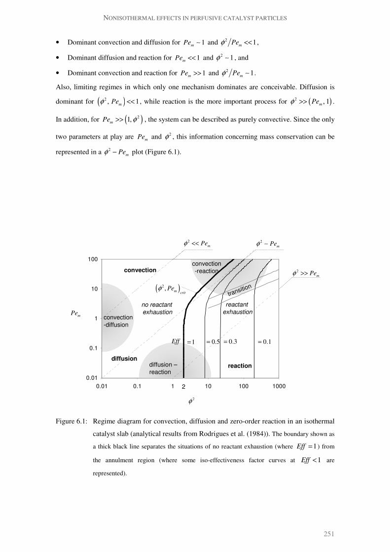
NONISOTHERMAL EFFECTS IN PERFUSIVE CATALYST PARTICLES
251
• Dominant convection and diffusion for 1m
Pe ∼ and 2 1m
Peφ << ,
• Dominant diffusion and reaction for 1m
Pe << and 2 1φ ∼ , and
• Dominant convection and reaction for 1m
Pe >> and 2 1m
Peφ ∼ .
Also, limiting regimes in which only one mechanism dominates are conceivable. Diffusion is
dominant for ( )2 , 1
mPeφ << , while reaction is the more important process for ( )
2 , 1m
Peφ >> .
In addition, for ( )21,
mPe φ>> , the system can be described as purely convective. Since the only
two parameters at play are m
Pe and 2φ , this information concerning mass conservation can be
represented in a 2m
Peφ − plot (Figure 6.1).
Figure 6.1: Regime diagram for convection, diffusion and zero-order reaction in an isothermal
catalyst slab (analytical results from Rodrigues et al. (1984)). The boundary shown as
a thick black line separates the situations of no reactant exhaustion (where 1Eff = ) from
the annulment region (where some iso-effectiveness factor curves at 1Eff < are
represented).
2m
Peφ ∼2
mPeφ <<
2m
Peφ >>
reactiondiffusion
convection
reactant
exhaustion
no reactant
exhaustion
2φ
mPe
diffusion –
reaction
convection
-diffusion
convection
-reaction
1=
2
( )2 ,
mcrit
Peφ
0.1=0.5= 0.3=Eff
transition
0.01
0.1
1
10
100
0.01 0.1 1 10 100 1000

CHAPTER 6
252
6.2.2.a Isothermal zero-order reaction in permeable catalyst slab
For an isothermal system, exact analytical solutions are available (Rodrigues et al. 1984). The
calculation of the effectiveness factor and the condition that separates the situation of reactant
exhaustion from the one where no concentration annulment occurs, are of particular interest.
These important results are represented in Figure 6.1. For representation convenience, we
choose a factor of 210− to express smallness in the above magnitude relations. The regions
where the system behaves globally as purely diffusive, convective or reactive are shown, as well
as the regimes described by a dominant balance between any of these two (grey areas). The
thick black line separates the parametric sets that lead to concentration annulment anywhere
inside the particle from the situations where no reactant exhaustion occurs. This line of
( )2 ,
mcrit
Peφ is also the iso-effectiveness factor curve for 1Eff = , when reactant concentration
reaches zero only at a single point inside the slab. For ( ) ( )2 2, ,
m mcrit
Pe Peφ φ< , no annulment
occurs and 1Eff = . Outside this region, catalyst performance decreases with increasing Thiele
modulus, according to the curves of constant effectiveness factor in the ( )2 ,
mPeφ plane. When
0m
Pe → , the boundary tends to the well-known diffusive limit of ( )2 2
critφ = , and for 2 2φ >
the iso-effectiveness factor curves approach the value 2Eff φ= . The effect of convection is
visible for high m
Pe , increasing the effectiveness factor for a given 2φ (and also the value of
( )2
critφ needed to achieve annulment), that is, the overall content in reactant inside the slab
increases. The region around the grey lines represent the transition zone, above which, the effect
of increasing the Peclet number (and therefore, convection) is particularly noticeable (this
approximated criteria will be derived in section 6.3.3.c).
6.2.2.b Scaling for temperature change in exothermic systems
In order to study nonisothermal systems, in which β and γ are fixed, we have to consider the
intraparticular heat Peclet number, h
Pe (through Lewis number, for example), in addition to 2φ
and m
Pe . A 3-D regime diagram can be constructed by adding this third axis (m h
Le Pe Pe= ),
as shown in Figure 6.2.
An order of magnitude estimation and scaling for the characteristic temperature change, T∆ ,
can be obtained by a balance between the terms corresponding to the dominant effects in the
energy balance (Lin et al. 1988). To compare the magnitude between all terms in equation (6.7)
we introduce a generic small parameter ε , which will express the relations between the

NONISOTHERMAL EFFECTS IN PERFUSIVE CATALYST PARTICLES
253
dimensionless groups. Therefore, for h
Pe ε∼ (reaction-conduction dominant balance),
2ˆad
T T Leφ∆ ∆ ∼ ; while for 1h
Pe ε−
∼ (strong heat convection balanced by reaction),
2ˆad m
T T Peφ∆ ∆ ∼ . When heat transport mechanisms dominate over reaction: 1h
Pe ∼ and
2ˆad m
T T Peφ∆ ∆ >> (we will take ( )2 1ˆ
ad mT T Peφ ε
−∆ ∆ ∼ ). In Figure 6.2a, the results of
temperature scaling in the planes of slow conduction ( )Le ε∼ , convection ( )mPe ε∼ and
reaction ( )2
φ ε∼ are indicated by: isothermal (when ( )ˆ ˆ ˆ,dif ad
T T T∆ << ∆ ∆ ); adiabatic
( ˆad
T T∆ ∆∼ ); diffusive ( ˆ ˆdif s
T Tβ∆ = ) and ‘explosion’ (if ( )ˆ ˆ ˆ,dif ad
T T T∆ >> ∆ ∆ ). In Figure 6.2b,
the 1m
Pe ε−
= and 2 1φ ε
−= planes are shown. Since for a given system, Lewis number is
approximately constant, we show in detail the planes for Le of order 1, ε and 1ε
− (Figure 6.3).
The boundaries between each region are schematic. The isothermal regions appear at regimes
where reaction is slow and heat removal by conduction/convection is strong. The parameter sets
where the characteristic temperature change is of the same order of the maximum temperature
change observed in a diffusive-reactive system with concentration annulment are related to the
ones leading to the adiabatic temperature change by the Lewis number, since ˆ ˆad dif
T T Le∆ = ∆ .
The indicated characteristic temperature changes are observed at an ( )1O scale inside the
catalyst and they account for the existence of reaction throughout the slab. However, the
existence of a reactant limitation (which puts an end to the heat-generating reaction) stops
temperature from becoming unbounded in the ‘explosion’ areas. Since no physical solution for
the steady-state mass and energy conservation equations (with the reaction term) can be found,
the proper form of (6.6)-(6.7) includes also the branch of ( ) 0r T = for ˆ 0c = .
To obtain a correct estimate for temperature change, ‘active’ regions of thickness much smaller
than 1 have to be considered (since the solution already includes an ( )1O branch from 24H(6.6)-
25H(6.7) with ( ) 0r T = ). If the thickness of these inner regions is χ for concentration and τ for
temperature, then we are interested in the cases where , 1χ τ << .
Rescaling x by χ and τ in the mass and energy conservation equations respectively, more
insight into the ‘explosive’ regions can be achieved, if we choose the consistent dominant
balances in each parameter set. So,
(a) For 1Le ∼ (Figure 6.3a) and 2 1φ ε
−∼ , diffusive-reactive inner regions with thickness
1χ φ ε
−∼ ∼ in the concentration profile and ˆ
difT Tτ ε ∆ ∆∼ in the temperature
profile are suggested. Since the two regions are comparable in extension ( χ τ∼ ), then
( )ˆ ˆ ˆdif ad
T T T∆ ∆ ∆∼ ∼ .

CHAPTER 6
254
(a) Le ε= , m
Pe ε= and 2φ ε= planes.
(b) 1m
Pe ε−
= and 2 1φ ε
−= planes.
Figure 6.2: 3-D regime diagram for convection, diffusion and exothermic reaction in a catalyst
slab. The regions marked as isothermal present very small deviation from surface
temperature. The adiabatic (ad.) limit is related with the characteristic temperature change
under diffusive conditions (diff., ˆ ˆdif s
T Tβ∆ = ) by the Lewis number: ˆ ˆad dif
T T Le∆ = ∆ .
When ˆ ˆ ˆ,ad dif
T T T∆ >> ∆ ∆ , ‘explosion’ (expl.) occurs.
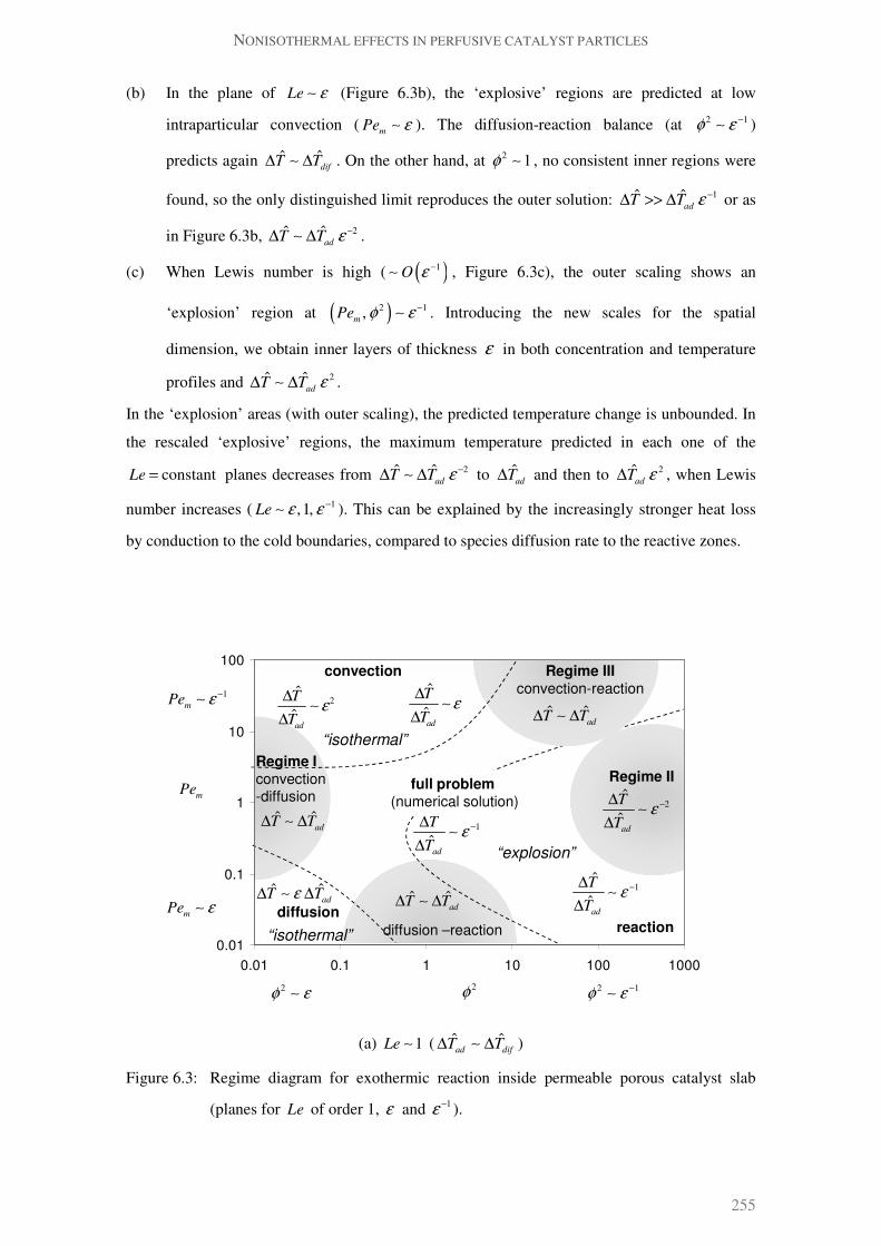
NONISOTHERMAL EFFECTS IN PERFUSIVE CATALYST PARTICLES
255
(b) In the plane of Le ε∼ (Figure 6.3b), the ‘explosive’ regions are predicted at low
intraparticular convection (m
Pe ε∼ ). The diffusion-reaction balance (at 2 1φ ε
−∼ )
predicts again ˆdif
T T∆ ∆∼ . On the other hand, at 2 1φ ∼ , no consistent inner regions were
found, so the only distinguished limit reproduces the outer solution: 1ˆad
T T ε−
∆ >> ∆ or as
in Figure 6.3b, 2ˆad
T T ε−
∆ ∆∼ .
(c) When Lewis number is high ( ( )1
O ε−
∼ , Figure 6.3c), the outer scaling shows an
‘explosion’ region at ( )2 1,
mPe φ ε
−∼ . Introducing the new scales for the spatial
dimension, we obtain inner layers of thickness ε in both concentration and temperature
profiles and 2ˆad
T T ε∆ ∆∼ .
In the ‘explosion’ areas (with outer scaling), the predicted temperature change is unbounded. In
the rescaled ‘explosive’ regions, the maximum temperature predicted in each one of the
constantLe = planes decreases from 2ˆad
T T ε−
∆ ∆∼ to ad
T∆ and then to 2ad
T ε∆ , when Lewis
number increases ( 1,1,Le ε ε−
∼ ). This can be explained by the increasingly stronger heat loss
by conduction to the cold boundaries, compared to species diffusion rate to the reactive zones.
(a) 1Le ∼ ( ˆ ˆad dif
T T∆ ∆∼ )
Figure 6.3: Regime diagram for exothermic reaction inside permeable porous catalyst slab
(planes for Le of order 1, ε and 1ε
− ).
2ˆ
ad
T
Tε
∆
∆∼
ˆ
ad
T
Tε
∆
∆∼
convection
“isothermal”
“explosion”
2φ
mPe
mPe ε∼
1m
Pe ε−
∼
2 1φ ε
−∼
2φ ε∼
1ˆ
ad
T
Tε
−∆
∆∼
Regime IIIconvection-reaction
reaction
ˆad
T Tε∆ ∆∼
diffusion
1ˆ
ad
T
Tε
−∆
∆∼
full problem (numerical solution)
Regime Iconvection-diffusion
2ˆ
ad
T
Tε
−∆
∆∼
Regime II
diffusion –reaction
ˆad
T T∆ ∆∼
“isothermal”
ˆad
T T∆ ∆∼
ˆad
T T∆ ∆∼
0.01
0.1
1
10
100
0.01 0.1 1 10 100 1000

CHAPTER 6
256
(b) Le ε∼ ( ˆ ˆad dif
T Tε∆ ∆∼ )
(c) 1Le ε
−∼ ( ˆ ˆ
dif adT Tε∆ ∆∼ )
Figure 6.3: Regime diagram for exothermic reaction inside permeable porous catalyst slab
(planes for Le of order 1, ε and 1ε
− ).
2ˆ
ad
T
Tε
∆
∆∼
ˆ
ad
T
Tε
∆
∆∼
convection
“isothermal”
“explosion”
2φ
mPe
mPe ε∼
1m
Pe ε−
∼
2 1φ ε
−∼
2φ ε∼
3ˆ
ad
T
Tε
−∆
∆∼
convection-reaction
reactionˆ
difT T∆ ∆∼
diffusion
convection
-diffusion
diffusion –reaction
ˆad
T T∆ ∆∼
ˆ
ad
T
Tε
∆
∆∼
ˆad
T T∆ ∆∼ˆ
difT T∆ ∆∼
2ˆ
ad
T
Tε
−∆
∆∼
0.01
0.1
1
10
100
0.01 0.1 1 10 100 1000
ˆdif
T T∆ ∆∼
convection
“explosion”
2φ
mPe
mPe ε∼
1m
Pe ε−
∼
2 1φ ε
−∼
2φ ε∼
ˆad
T T∆ ∆∼
convection-reaction
reactionconduction
convection
-diffusion
diffusion –reaction
1ˆad
T T ε−
∆ ∆∼
2ˆad
T T ε∆ ∆ ∼
ˆdif
T T∆ ∆∼
ˆdif
T T∆ ∆∼
ˆad
T T∆ ∆∼
ˆad
T T∆ ∆∼
“isothermal”
0.01
0.1
1
10
100
0.01 0.1 1 10 100 1000

NONISOTHERMAL EFFECTS IN PERFUSIVE CATALYST PARTICLES
257
Since the remaining of this work focuses on the particular case of 1Le ∼ (Figure 6.3a) we take
adT∆ as a scale for temperature change in the regimes of slow and fast reaction (Regime I and II
respectively) and strong intraparticular convection (Regime III). We can also anticipate that in
Regime II, non-uniformities will arise. With this scale, equations (6.6)-(6.7) become:
( )
2 2
2
1
m m
dc d cr T
dx Pe dx Pe
φ= − (6.17)
( )
2 2
2
1m
m h m
PedT d Tr T
dx Pe Pe dx Pe
φ= + (6.18)
The reaction term was assumed of ( )1O :
( ) [ ]exp exp exp1 1
T LeTr T LeT
T LeT
ϕ γ βγ β
η β
= =
+ + ∼
for Le and ( )1T O∼ . The product γ β can also be taken close to unity for common exothermic
reactions, since β rarely exceeds 0.3 and the typical range for γ is 10 30−∼ (Rodrigues 1981).
6.3 PERTURBATION ANALYSIS
The limiting cases discussed in the previous section can be analysed in more depth by
considering appropriate parameter regimes and conducting a perturbation analysis (Bender et al.
1999). This involves the choice of a perturbation (small) parameter ε , against which all others
should be compared. Concentration and temperature profiles are expanded as series of powers
of ε and substituted into the governing differential equations and boundary conditions. An
infinite set of determined problems is obtained when terms of the same order are collected in
each equation. The leading-order problem reflects the assumed dominant balance, while higher
order corrections account for the negligible mechanism. The results in the present work apply to
( )1Le O∼ and they intend to approximate the full solution of the complete problem in the limits
of: fast mass/heat transport (Regime I), dominant reaction (Regime II) and strong intraparticular
convection (Regime III). The diffusive regime for an exothermic zero-order reaction (diffusion-
reaction grey area in Figure 6.3 and 0m
Pe = plane in Figure 6.2a) was studied, among others,
by Frank-Kamenetskii (1955), Hlavacek (1967) and Aris (1975) and it will be used to validate
our solutions.

CHAPTER 6
258
Figure 6.4: Schematic concentration and temperature profiles in a permeable catalyst slab,
where an exothermic zero-order reaction occurs. The regimes studied are: slow and
fast reaction (Regime I and II, respectively) and strong convection with and without
(Regime IIIb and Regime IIIa, respectively) concentration annulment.
6.3.1 Regime I (Chemical regime)
When transport mechanisms are much faster than chemical reaction, concentration and
temperature inside the slab depart little from its surface values (Figure 6.4). This corresponds to
the case when Thiele modulus is low and to the classic chemical regime, in the presence of
convection.
Assuming that the terms in Eqs.28H(6.17)-29H(6.18) are correctly scaled, we take 2m
Peε φ= as
perturbation parameter and look for outer solutions (valid in ( )1x O= ) under the following
conditions:
2 1 11, ,
m m hPe Pe Pe
φ<< (6.19)
Also, in this regime, concentration annulment is not expected to occur, so the appropriate form
of mass and energy balances takes into account the reaction term:
ˆs
cI
IIIa
IIIb
II
c = 0
L
u
ˆs
TI
IIIa
IIIb
IIT
c
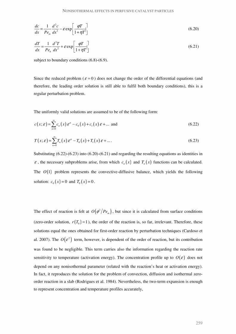
NONISOTHERMAL EFFECTS IN PERFUSIVE CATALYST PARTICLES
259
2
2
1exp
1m
dc d c T
dx Pe dx T
ϕε
η
= −
+ (6.20)
2
2
1exp
1h
dT d T T
dx Pe dx T
ϕε
η
= +
+ (6.21)
subject to boundary conditions 30H(6.8)-31H(6.9).
Since the reduced problem ( 0ε = ) does not change the order of the differential equations (and
therefore, the leading order solution is still able to fulfil both boundary conditions), this is a
regular perturbation problem.
The uniformly valid solutions are assumed to be of the following form:
( ) ( ) ( ) ( )0 10
; ...n
n
n
c x c x c x c xε ε ε
∞
=
= + +∑ ∼ and (6.22)
( ) ( ) ( ) ( )0 10
; ...n
n
n
T x T x T x T xε ε ε
∞
=
= + +∑ ∼ . (6.23)
Substituting 32H(6.22)-33H(6.23) into 34H(6.20)-35H(6.21) and regarding the resulting equations as identities in
ε , the necessary subproblems arise, from which ( )nc x and ( )n
T x functions can be calculated.
The ( )1O problem represents the convective-diffusive balance, which yields the following
solution: ( )0 0c x = and ( )0 0T x = .
The effect of reaction is felt at ( )2
mO Peφ , but since it is calculated from surface conditions
(zero-order solution, ( )0 1r T = ), the order of the reaction is, so far, irrelevant. Therefore, these
solutions equal the ones obtained for first-order reaction by perturbation techniques (Cardoso et
al. 2007). The ( )2
O ε term, however, is dependent of the order of reaction, but its contribution
was found to be negligible. This term carries also the information regarding the reaction rate
sensitivity to temperature (activation energy). The concentration profile up to ( )O ε does not
depend on any nonisothermal parameter (related with the reaction’s heat or activation energy).
In fact, it reproduces the solution for the problem of convection, diffusion and isothermal zero-
order reaction in a slab (Rodrigues et al. 1984). Nevertheless, the two-term expansion is enough
to represent concentration and temperature profiles accurately,

CHAPTER 6
260
( )
( )1 22 4
2 2 2
2 1
1 1
m m
m m
Pe x Pe
Pe Pe
m m
e ec x x O
Pe Pee e
φ φ+ +
= − − + − −
(6.24)
( )
( )1 22 4
2 2 2
2 1
1 1
h h
h h
Pe x Pe
Pe Pe
m m
e eT x x O
Pe Pee e
φ φ+ +
= + + + − −
. (6.25)
Concentration and temperature profiles (Eqs.36H(6.24) and 37H(6.25)) are represented in Figure 6.5.
Numerical results obtained with gPROMS (2007) are also plotted. The agreement is especially
good for 0.01ε ∼ .
For an exothermic reaction, the maximum temperature occurs at:
2
max
1 11 ln
2
hPe
h h
ex
Pe Pe
−= − +
(6.26)
while the minimum concentration position is
2
min
1 11 ln
2
mPe
m m
ex
Pe Pe
−= − +
. (6.27)
which is, in general, distinct from maxx (as long as 1Le ≠ ). The minimum concentration value in
this regime is of order ε , and is given by:
22min
2
2 1 1 1ln
21
m
m
Pe
Pe
m m m m
ec
Pe Pe Pe Pee
φ −= − − +
− (6.28)
Since thermal effects do not affect the concentration profile for weak reaction conditions,
equations 38H(6.27) and 39H(6.28) reproduce the isothermal results (Rodrigues et al. 1984), when no
annulment occurs. An estimate for maximum temperature will be given in section 6.4.
Although the dominant balance requires that 1m
Pe ∼ and 1h
Pe ∼ , we expect that the presented
solutions can also include the regimes where convection or diffusion is the only important
mechanism. In the chemical regime, the limits of strong convection ( , 1m h
Pe Pe >> ) or diffusion
( , 1m h
Pe Pe << ) yield both: ( ) ( ), 0c x T x → . However, convective transport suggests profile
asymmetry ( min max, 1x x → ), in contrast with the symmetry characteristic of diffusive profiles
( min max, 0x x → ).

NONISOTHERMAL EFFECTS IN PERFUSIVE CATALYST PARTICLES
261
(a) Reactant concentration profile.
(b) Temperature profile.
Figure 6.5: Comparison of the perturbation solutions (equations 40H(6.24)-41H(6.25), dashed lines)
with numerical results from gPROMS® (solid lines) for 20γ = , 0.1β = ,
10m
Pe = , 5h
Pe = , and 2 0.1φ = ( 0.01ε = ) or 2 0.5φ = ( 0.05ε = ).
0.9
0.92
0.94
0.96
0.98
1
-1 -0.8 -0.6 -0.4 -0.2 0 0.2 0.4 0.6 0.8 1
2 0.1φ =
2 0.5φ =
ˆx x L=
ˆ
ˆs
c
c
1
1.005
1.01
1.015
1.02
-1 -0.8 -0.6 -0.4 -0.2 0 0.2 0.4 0.6 0.8 1
2 0.1φ =
2 0.5φ =
ˆx x L=
ˆ
s
T
T

CHAPTER 6
262
6.3.2 Regime II (Diffusional regime)
The regime in which reaction is fast compared with transport mechanisms appears for large
Thiele modulus. In order to study this diffusional regime (in the presence of convection), we set
the perturbation parameter to: 2m
Peε φ= . Under the conditions:
2 1 11, ,
m m hPe Pe Pe
φ>> (6.29)
the solution to 42H(6.17)-43H(6.18) is obtained by conducting a singular perturbation analysis, since
keeping the original scaling does not yield an uniformly valid result. We expect boundary layers
to occur near the slab surfaces, where reactant concentration decreases and temperature
increases sharply from the middle solution to surface values (Figure 6.4).
6.3.2.a Middle region
Looking for an outer solution with mass/energy equations that include chemical reaction leads
to an ( )1O problem with no physical solution. That is, the reduced problem from
2
2exp
1
m m m
m
m
dc d c T
dx Pe dx T
ε ϕε
η
= −
+ (6.30)
2
2exp
1
m m m
m
h
dT d T T
dx Pe dx T
ε ϕε
η
= +
+ (6.31)
suggests that concentration and thermal boundary layers will develop at x L= ± (as no
boundary conditions can be fulfilled) and since ( )exp 1 0m mT Tϕ η + = is not possible, this
should correspond to a ‘dead core’ situation where reactant vanishes and ‘explosion’ occurs.
Consequently, chemistry-free equations should be used in this region. They are written as:
( ) 1mc x = − for ' *x x x≤ ≤ (6.32)
2
2
1m m
h
dT d T
dx Pe dx= for ' *x x x≤ ≤ . (6.33)
The solution from 44H(6.33) is intended to represent the temperature profile in the region where
reactant disappears (between 'x and *x ). This equation is valid for all orders of the
perturbation parameter and is free of ε . Therefore, all subproblems of order ( )/2n
O ε arising
from 45H(6.33) are identical and the expansion for the temperature profile in the middle section of
the slab is:

NONISOTHERMAL EFFECTS IN PERFUSIVE CATALYST PARTICLES
263
( ) ( )/2 /2
0 0
; hPe xm m n nn
n n
n n h
hT x T x e j
Peε ε ε
∞ ∞
= =
= = +
∑ ∑ for ' *x x x≤ ≤ . (6.34)
The shape of the temperature profile is exponentially increasing / decreasing or a plateau,
depending on the value of ( )/ 2
0
hPe xm n
n
n
d T d x h e ε
∞
=
=∑ ( 0hPe xe > , so the sign of m
d T d x is
independent of x ). Since the nature of the regions at 1x = ± is such that surface temperature is
brought monotonically to match the middle region profile, we expect that the derivative of these
solutions to be null either at 'x or *x (where the maximum temperature occurs). These regions
are described by equations 46H(6.30)-47H(6.31), which are fundamentally different from 48H(6.32)-49H(6.33).
Therefore, we use perturbation analysis as an approximation procedure for boundary layers and
require profile and flux continuity with the middle region. As a result of both derivative
continuity and concentration annulment at 'x and *x , Eq. 50H(6.34) has to predict a plateau with
no temperature variation in the middle of the slab. This is a reasonable simplification for the
conditions defined in this regime, and is confirmed by numerical simulations for the first-order
reaction case (Quinta Ferreira 1988). Consequently, the maximum temperature is:
( ) ( ) ( )max max max
0 1;mT x T T T Oε ε ε ε= = + + . (6.35)
6.3.2.b Right boundary layer
At the inner layer near 1x = , the following stretching transformation is introduced:
1 xX
δ
−= . (6.36)
The boundary layer thickness (δ ) correctly rescales the convective, diffusive and reactive
terms. A dominant balance between two of these terms yields the distinguished limit. In this
case, the consistent option is a reaction-diffusion balance (δ ε∼ ), being convection only
important at ( )O ε . Equations 51H(6.30)-52H(6.31) then become:
2
2
1exp 0
1
r r r
r
m
d c dc T
Pe dX dX T
ϕε
η
+ − =
+ for 0 *X X≤ ≤ (6.37)
2
2
1exp 0
1
r r r
r
h
d T dT T
Pe dX dX T
ϕε
η
+ + =
+ for 0 *X X≤ ≤ (6.38)
with boundary conditions:
( )0 0rc X = = and (6.39)
( )0 0rT X = = . (6.40)

CHAPTER 6
264
Equations 53H(6.37) and 54H(6.38) suggest that we look for solutions of the form:
( ) ( )/2
0
r r n
n
n
c x c x ε
∞
=
=∑ and (6.41)
( ) ( )/2
0
r r n
n
n
T x T x ε
∞
=
=∑ (6.42)
where ( ) ( )r r
n nc x c X≡ , ( ) ( )
r r
n nT x T X≡ and ( )* 1 *X x ε= − .
6.3.2.c Left boundary layer
At the slab’s ‘entrance’, the proper rescaling is given by:
1 xY
ε
+= (6.43)
predicted from the diffusive-reactive nature of the boundary layer (same reasoning as for the
boundary layer on the right). The equations for this region are:
2
2
1exp 0
1
l l l
l
m
d c dc T
Pe dY dY T
ϕε
η
− − =
+ for 0 'Y Y≤ ≤ (6.44)
2
2
1exp 0
1
l l l
l
h
d T dT T
Pe dY dY T
ϕε
η
− + =
+ for 0 'Y Y≤ ≤ (6.45)
subject to:
( )0 0lc Y = = and (6.46)
( )0 0lT Y = = . (6.47)
The form of the solutions that we are looking for is, again:
( ) ( )/2
0
l l n
n
n
c x c x ε
∞
=
=∑ and (6.48)
( ) ( )/2
0
l l n
n
n
T x T x ε
∞
=
=∑ (6.49)
where ( ) ( )l l
n nc x c Y≡ , ( ) ( )
l l
n nT x T Y≡ and ( )' 1 'Y x ε= − + .

NONISOTHERMAL EFFECTS IN PERFUSIVE CATALYST PARTICLES
265
6.3.2.d Profile and flux continuity at *x and 'x
The problem is completely determined if two more types of conditions are provided: one from
where the positions *X and 'Y can be calculated, and the remaining boundary condition for the
problems defined by 55H(6.37)-56H(6.40) and 57H(6.44)-58H(6.47). Conditions for profile continuity at each
order of the small parameter can be written as:
( ) ( )1, 0
* *0, 1
r m
n n
nc X c x
n
− == =
≥ (6.50)
and ( ) ( )max* *r m
n n nT X T x T= = (6.51)
at the right boundary layer, and
( ) ( )1, 0
' '0, 1
l m
n n
nc Y c x
n
− == =
≥ (6.52)
and ( ) ( )max' 'l m
n n nT Y T x T= = (6.53)
at the left one.
To determine the annulment positions from gradient continuity between the boundary layers and
the middle region, we have to solve nonlinear algebraic equations in *X and 'Y . An explicit
approximate solution can be found if we expand these unknowns as:
( )/2
0 10
** * *n
n
n
X X X X Oε ε ε
∞
=
= = + +∑ and (6.54)
( )/2
0 10
'' ' 'n
n
n
Y Y Y Y Oε ε ε
∞
=
= = + +∑ . (6.55)
After linearization around 0ε = , the coefficients *n
X and 'n
Y for ( 0, 1n = ) can be determined
from:
0*,
lim 0r
X
dc
dXε
ε
→
= (6.56)
0',
lim 0l
Y
dc
dYε
ε
→
= (6.57)
0*, *, 0
1lim 0
r r
X X
dc dc
dX dXε
ε εε→
=
− =
(6.58)
0', ', 0
1lim 0
l l
Y Y
dc dc
dY dYε
ε εε→
=
− =
. (6.59)
The problem is closed when the same equations are written for the temperature profile, and the
coefficients in equation 59H(6.35) can then be determined (maximum temperature estimate).

CHAPTER 6
266
6.3.2.e Approximate concentration and temperature profiles
If expansions 60H(6.41)-61H(6.42) and 62H(6.48)-63H(6.49) are substituted into the equations for the boundary
layers (64H(6.37)-65H(6.40) and 66H(6.44)-67H(6.47)), and we collect same order terms, a sequence of sub-
problems is obtained. The nonlinear term 68H(6.10) is expressed by a Taylor series around 0ε = .
At ( )1O the problem reduces to the following set of equations for the right boundary layer
( * 1x x< < ):
20 02
0
1exp 0
1
r r
r
m
d c T
Pe dX T
ϕ
η
− =
+ and (6.60)
20 02
0
1exp 0
1
r r
r
h
d T T
Pe dX T
ϕ
η
+ =
+ for 0 *X X≤ ≤ (6.61)
with boundary conditions given by 69H(6.39)-70H(6.40) and 71H(6.50)-72H(6.51) for 0n = . Adding both
equations, the well-known Damköhler relation in the diffusive limit is obtained, if the maximum
temperature is max0 h m
T Pe Pe= (in dimensional variables: ( )maxˆ ˆ 1
sT T β= + ):
( )0 0r r
h mT Pe Pe c= − (6.62)
(or, in dimensional variables: ( )0 0ˆ ˆ ˆ ˆ1 1r r
s sT T c cβ= + − ).
A similar leading-order problem can be extracted from the left boundary layer equations (73H(6.44)-
74H(6.47) and 75H(6.52)-76H(6.53)). Both these problems find simple analytical solution under the
simplification:
20
0
exp1
r
r
Tb
T
ϕ
η
+ ≃ (6.63)
The constant 2b will be determined later by an integral approximation. Also, from equations
77H(6.56)-78H(6.57), 0 *X and 0 'Y can be estimated. Those results are written as:
( ) ( )
2
0 ** 2
r mPe bX
c X X X XX
= − + − (6.64)
( ) ( )
2max
0 0 ** 2
r hPe bX
T X T X X XX
= − − and (6.65)
( ) ( )
2
0 '' 2
l mPe bY
c Y Y Y YY
= − + − (6.66)
( ) ( )
2max
0 0 '' 2
l hPe bY
T Y T Y Y YY
= − − (6.67)
with,

NONISOTHERMAL EFFECTS IN PERFUSIVE CATALYST PARTICLES
267
max0
h
m
PeT
Pe= , (6.68)
0 2
2*
m
XPe b
= and (6.69)
0 2
2'
m
YPe b
= . (6.70)
The ( )O ε problem takes into consideration the convective term influence. In the right
boundary layer ( * 1x x< < ), mass and energy conservation equations write as:
( )
20 01
12200
1exp
11
r rr
r
rr
m
T dcd cT
Pe dX T dXT
ϕϕ
ηη
− = −
+ +
and (6.71)
( )
20 01
12200
1exp
11
r rr
r
rr
h
T dTd TT
Pe dX T dXT
ϕϕ
ηη
+ = −
+ +
for 0 *X X≤ ≤ . (6.72)
with 79H(6.39)-80H(6.40) and 81H(6.50)-82H(6.51) as boundary conditions ( 1n = ). The corresponding problem
at the left boundary layer appears from equations 83H(6.44)-84H(6.47) and 85H(6.52)-86H(6.53). In order to
find a simple solution, the following simplifications are made:
( )
012
00
exp11
rr
rr
TTd
TT
ϕϕ
ηη
+ +
≃ (6.73)
( )
012
00
exp11
ll
ll
TTf
TT
ϕϕ
ηη
+ +
≃ (6.74)
Constants d and f will be estimated by an integral approximation. Finally, concentration and
temperature profile corrections at ( )O ε are:
( ) ( )
2
1
** *
2 3 2r m m
Pe b Pe Xc X X X X X d X
= − + − −
(6.75)
( ) ( )
max 2max 0
1 1
** * *
* 2 2 6 2r h
h
T b PeX d XT X T Pe X X X X X
X
= − − + + − +
(6.76)
and
( ) ( )
2
1
1 ''
2 ' 3 2l m m
Pe Y b Pe Yc Y Y Y f Y
Y
= − − + + −
(6.77)
( ) ( )
max 2max01
1
''
' 2 ' 2 6 2l m
h
T b PeT f YT Y Y Pe Y Y Y
Y Y
= − − − + + −
(6.78)
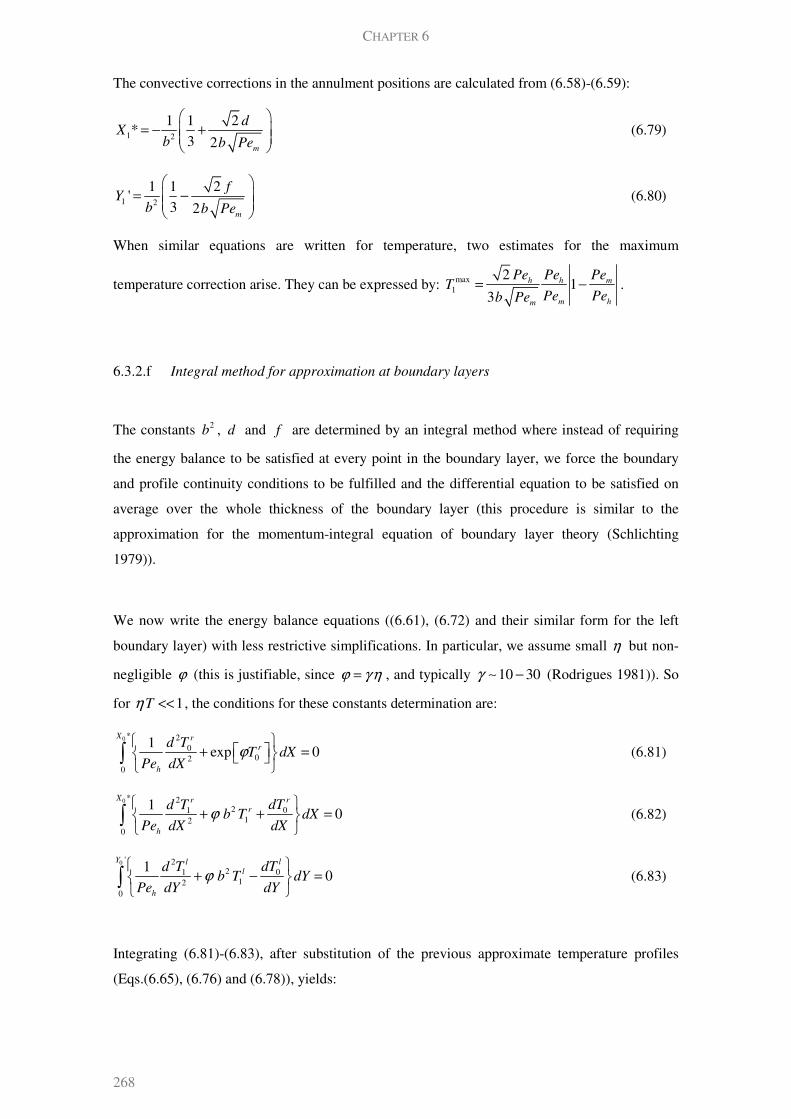
CHAPTER 6
268
The convective corrections in the annulment positions are calculated from 87H(6.58)-88H(6.59):
1 2
1 1 2*
3 2m
dX
b b Pe
= − +
(6.79)
1 2
1 1 2'
3 2m
fY
b b Pe
= −
(6.80)
When similar equations are written for temperature, two estimates for the maximum
temperature correction arise. They can be expressed by: max1
21
3h h m
m hm
Pe Pe PeT
Pe Peb Pe= − .
6.3.2.f Integral method for approximation at boundary layers
The constants 2b , d and f are determined by an integral method where instead of requiring
the energy balance to be satisfied at every point in the boundary layer, we force the boundary
and profile continuity conditions to be fulfilled and the differential equation to be satisfied on
average over the whole thickness of the boundary layer (this procedure is similar to the
approximation for the momentum-integral equation of boundary layer theory (Schlichting
1979)).
We now write the energy balance equations (89H(6.61), 90H(6.72) and their similar form for the left
boundary layer) with less restrictive simplifications. In particular, we assume small η but non-
negligible ϕ (this is justifiable, since ϕ γ η= , and typically 10 30γ −∼ (Rodrigues 1981)). So
for 1Tη << , the conditions for these constants determination are:
0 * 20
020
1exp 0
X r
r
h
d TT dX
Pe dXϕ
+ =
∫ (6.81)
0 * 22 01
120
10
X rr
r
h
dTd Tb T dX
Pe dX dXϕ
+ + =
∫ (6.82)
0 ' 22 01
120
10
Y ll
l
h
dTd Tb T dY
Pe dY dYϕ
+ − =
∫ (6.83)
Integrating 91H(6.81)-92H(6.83), after substitution of the previous approximate temperature profiles
(Eqs.93H(6.65), 94H(6.76) and 95H(6.78)), yields:
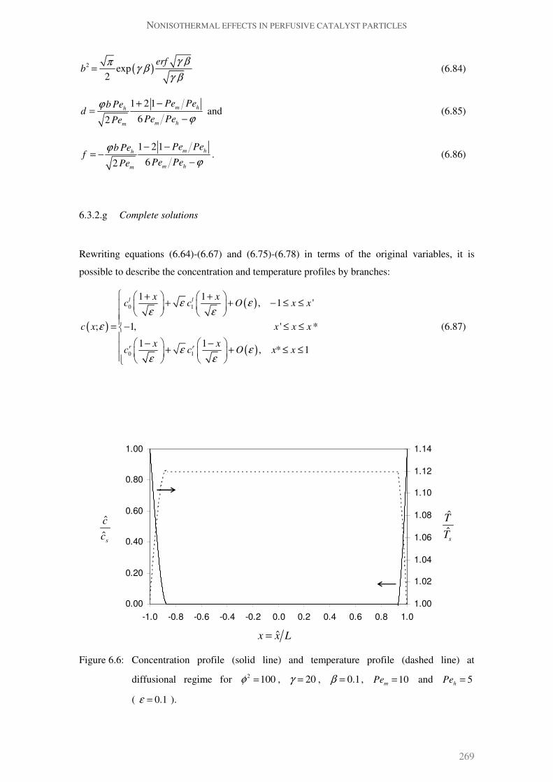
NONISOTHERMAL EFFECTS IN PERFUSIVE CATALYST PARTICLES
269
( )2 exp
2
erfb
γ βπγ β
γ β= (6.84)
1 2 1
62m hh
m hm
Pe Peb Ped
Pe PePe
ϕ
ϕ
+ −=
− and (6.85)
1 2 1
62m hh
m hm
Pe Peb Pef
Pe PePe
ϕ
ϕ
− −= −
−. (6.86)
6.3.2.g Complete solutions
Rewriting equations 96H(6.64)-97H(6.67) and 98H(6.75)-99H(6.78) in terms of the original variables, it is
possible to describe the concentration and temperature profiles by branches:
( )
( )
( )
0 1
0 1
1 1, 1 '
; 1, ' *
1 1, * 1
l l
r r
x xc c O x x
c x x x x
x xc c O x x
ε εε ε
ε
ε εε ε
+ + + + − ≤ ≤
= − ≤ ≤
− − + + ≤ ≤
(6.87)
Figure 6.6: Concentration profile (solid line) and temperature profile (dashed line) at
diffusional regime for 2 100φ = , 20γ = , 0.1β = , 10m
Pe = and 5h
Pe =
( 0.1ε = ).
0.00
0.20
0.40
0.60
0.80
1.00
-1.0 -0.8 -0.6 -0.4 -0.2 0.0 0.2 0.4 0.6 0.8 1.0
1.00
1.02
1.04
1.06
1.08
1.10
1.12
1.14
ˆ
s
T
T
ˆ
ˆs
c
c
ˆx x L=

CHAPTER 6
270
( )
( )
( )
( )
0 1
max
0 1
1 1, 1 '
; , ' *
1 1, * 1
l l
r r
x xT T O x x
T x T x x x
x xT T O x x
ε εε ε
ε ε
ε εε ε
+ + + + − ≤ ≤
= ≤ ≤
− − + + ≤ ≤
. (6.88)
The concentration annulment positions are calculated from 100H(6.69)-101H(6.70) and 102H(6.79)-103H(6.80):
( ) ( )3/2
0 1* 1 * 1 * *x X X X Oε ε ε ε= − = − + + and (6.89)
( ) ( )3/2
0 1' 1 ' 1 ' 'x Y Y Y Oε ε ε ε= − + = − + + + (6.90)
Solutions 104H(6.87)-105H(6.88) are presented in Figure 6.6.
The leading-order problem in the boundary layers (e.g., Eqs.106H(6.60)-107H(6.61) for the right boundary
layer) assumes a reaction-diffusion dominant balance, so the solution given by 108H(6.64)-109H(6.70) and
110H(6.84) can be directly compared with the exact analytical solutions at high Thiele modulus for
the problem of exothermic zero-order reaction in a catalyst slab where mass/heat transfer occurs
solely by diffusion/conduction. In particular, we compare concentration and temperature
profiles (or simply temperature profiles, since for this order, they are both related by Eq. 111H(6.62))
and concentration annulment points.
For slab geometry, when 2 0.878γ β φ > (at high Thiele modulus), there is only one steady state
solution for the diffusive-reactive problem (Frank-Kamenetskii 1955; Marek et al. 1968; Aris
1975) with
( )
1 /22 sech* ' 1
ex x
e
γ β
γ βφ γ β
− −
= − = − (6.91)
This result agrees with our perturbation solutions 112H(6.69)-113H(6.70) if ( )1 /2sechb e e
γ β γ βγ β
− −∼ ,
with b from 114H(6.84). This comparison is plotted in Figure 6.7 for several values of γ β .
At high Thiele modulus, the temperature and concentration variation is concentrated in thin
boundary layers, so the parabolic approximation 115H(6.64)-116H(6.67) is a reasonable one, which proves
to be in excellent agreement with exact analytical results (Aris 1975), as shown in Figure 6.8.
The leading-order temperature profile in the middle region (Eq.117H(6.68)) is Prater’s maximum
temperature estimate for reaction-diffusion problems.
NONISOTHERMAL EFFECTS IN PERFUSIVE CATALYST PARTICLES
271
Figure 6.7: Concentration annulment positions in the diffusive limit for an exothermic zero-
order reaction. Comparison between the exact analytical solution (Aris 1975) and
perturbation solutions in the limit of negligible convection (Eqs. 118H(6.69)-119H(6.70) with 120H(6.84)).
For 0.1γ β ≤ , exact and approximate results coincide.
Figure 6.8: Temperature profiles in the right boundary layer (next to 1x = ) in the diffusional
regime for 20γ = , 0.1β = , 10m
Pe = and 5h
Pe = and 10,50,100φ = . The
leading-order perturbation solutions (dashed lines) are compared with the exact analytical
results (solid lines) by e.g. Aris (1975).
0,5
0,6
0,7
0,8
0,9
1,0
10 100 1000
Approximate
Exact
0γ β =
0.1γ β =
5=
2=
1=
* 'x x= −
2φ
1,00
1,02
1,04
1,06
1,08
1,10
0,93 0,94 0,95 0,96 0,97 0,98 0,99 1,00
Exact
Approximate
2 210φ =
2 250φ =
2 2100φ =
ˆ
s
T
T
ˆx x L=

CHAPTER 6
272
In the isothermal limit ( 0ϕ → , 2 1b → and , 0d f → ), equations 121H(6.89)-122H(6.90) yield
( )3/22 1
* 13
m
x OPe
ε ε ε→ − + + (6.92)
( )3/22 1
' 13
m
x OPe
ε ε ε→ − + + + (6.93)
In the analysis of convection and diffusion with zero-order isothermal reaction, Rodrigues et al.
(1984) calculate *x and 'x by solving numerically two nonlinear algebraic equations. We can
find an approximate solution for those equations by perturbation techniques, for
2 1m
Peε φ= << . The result of that calculation reproduces equations 123H(6.92)-124H(6.93).
6.3.3 Regime III (Strong intraparticular convection regime)
A third regime, where intraparticular convection dominates mass and heat transport, can be
studied for parameters obeying the following conditions:
2
1m
Pe
φ∼ and
1 1, 1
h mPe Pe
<< (6.94)
Therefore, 1m
Peε = is taken as the perturbation parameter (also 1h
Pe ε∼ ). Since the reaction
term in equation 125H(6.10) is defined by two branches, the situation with concentration annulment
(section 6.3.3.b) needs to be treated separately from the one where no reactant exhaustion
occurs (section 6.3.3.a).
6.3.3.a No annulment of reactant concentration inside the particle (Regime IIIa)
Since reactant exhaustion never occurs within the slab (Figure 6.4), the mass and energy
equations with their original scaling ( x , ( )c x and ( )T x are assumed to be of ( )1O ) are:
2 2
2exp
1
l l l
l
m
dc d c T
dx dx Pe T
φ ϕε
η
= −
+ (6.95)
2 2
2exp
1
l l l
m
l
h m
PedT d T T
dx Pe dx Pe T
φ ϕε
η
= +
+ (6.96)
When ( )l
c x and ( )l
T x in equations 126H(6.95) and 127H(6.96) are expanded as a series in terms of
powers of the small parameter, the leading-order problem (obtained setting 0ε = ) is reduced to
a first order ODE, which is in general, not able to fulfil both boundary conditions. In the thin

NONISOTHERMAL EFFECTS IN PERFUSIVE CATALYST PARTICLES
273
region next to the abandoned condition, a boundary layer will appear, bringing the concentration
and temperature outer profiles to surface values. The only consistent option for matching
between such two solutions is to drop the condition next to 1x = . Equations 128H(6.95)-129H(6.96)
should then be solved with:
( )0 1 0lc x = − = and (6.97)
( )0 1 0lT x = − = (6.98)
For 0 1lTη << , the solution for the left/middle region of the slab is
( )
2
0
1ln 1 1l
m
T xPe
ϕφ
ϕ
= − − +
(6.99)
( )
2
0 0
1ln 1 1l l
m
c T xPe
ϕφ
ϕ
= − = − +
. (6.100)
Because solutions 130H(6.99)-131H(6.100) have a vertical asymptote, the existence of a bounded solution
requires that ( )
2
1 1m
xPe
ϕφ+ < .
Boundary layer next to 1x =
To investigate the nature of the inner region near the slab’s right surface, we introduce the
following stretching transformation: ( )1Y x δ= − . Comparing the substituted terms in
equations 132H(6.95) and 133H(6.96), the distinguished limit (that doesn’t reproduce the outer expansion)
is a convective-diffusive balance in a thin layer of thickness δ ε∼ . We will therefore calculate
concentration and temperature profiles based on expansions of the form:
( ) ( )0
n
n
n
c x c x ε
∞
=
=∑ and (6.101)
( ) ( )0
n
n
n
T x T x ε
∞
=
=∑ . (6.102)
The inner problem can be written as:
2 2
2exp
1
r r r
r
m
dc d c T
dY dY Pe T
φ ϕε
η
− = −
+ (6.103)
2 2
2exp
1
r r r
m
r
h m
PedT d T T
dY Pe dY Pe T
φ ϕε
η
− = +
+ (6.104)
with boundary conditions:

CHAPTER 6
274
( )0 0rc Y = = and ( )0 0r
T Y = = (6.105)- (6.106)
Substituting expansions 134H(6.101)-135H(6.102) into the problem defined by 136H(6.103)-137H(6.106) and
collecting ( )1O terms, the leading-order solution is:
( ) ( )0 1 1 exprc Y a Y= − − (6.107)
( )0 2 1 expr h
m
PeT Y a Y
Pe
= − −
. (6.108)
Integration constants 1a and 2a will be determined by matching with the outer solution 138H(6.99)-
139H(6.100). With ( )1O terms, the matching principle is simply (Bender et al. 1999):
0 01
lim limr l
Y x
c c→∞ →
= (6.109)
0 01
lim limr l
X x
T T→∞ →
= . (6.110)
Taking the limits of equations 140H(6.99), 141H(6.100), 142H(6.107) and 143H(6.108):
2
1 2
1 2ln 1
m
a aPe
ϕ φ
ϕ
= − = −
(6.111)
Matching between the two solutions is possible only if:
221
mPe
ϕφ< . (6.112)
If condition 144H(6.112) is not met then a solution valid for the whole slab cannot be obtained. This
suggests that, for typical parameter values, these solutions are only suitable for low Thiele
modulus range. They will be useful for describing a regime near the ‘chemical regime’, but with
strong convection. An additional term was calculated at ( )O ε , but it was found to have
negligible contribution to the complete solution.
Composite solution
The final composite solution, valid across the whole catalyst, is given by
( ) ( ) ( )( ) ( )0 0 0 01 limcomp l r r
mY
c x c x c Pe x c Y→∞
= + − − (6.113)
( ) ( ) ( )( ) ( )0 0 0 01 limcomp l r r
mY
T x T x T Pe x T Y→∞
= + − − (6.114)
Substituting 145H(6.99)-146H(6.100) and 147H(6.107)-148H(6.108) into 149H(6.113)-150H(6.114):
( )( )
2 211 1 2 1
( ) ln 1 1 ln 1 mPe x
m m m
c x x e OPe Pe Pe
ϕφ ϕφ
ϕ ϕ
− −
= − + − − +
(6.115)

NONISOTHERMAL EFFECTS IN PERFUSIVE CATALYST PARTICLES
275
(a) Reactant concentration profile.
(b) Temperature profile.
Figure 6.9: Comparison between composite solutions 161H(6.115)-162H(6.116), numerical results and
contributions from outer and inner regions for 4ϕ = , 2 20.8φ = , 10m
Pe = and
5h
Pe = .
0.80
0.85
0.90
0.95
1.00
-1.0 -0.8 -0.6 -0.4 -0.2 0.0 0.2 0.4 0.6 0.8 1.0
Composite solution
Numerical
Outer solution
Inner solution
ˆ
ˆs
c
c
ˆx x L=
1.00
1.01
1.02
1.03
1.04
1.05
-1.0 -0.8 -0.6 -0.4 -0.2 0.0 0.2 0.4 0.6 0.8 1.0
Composite solution
Numerical
Outer solution
Inner solutionˆ
s
T
T
ˆx x L=

CHAPTER 6
276
( )( )
2 211 1 2 1
( ) ln 1 1 ln 1 hPe x
m m m
T x x e OPe Pe Pe
ϕφ ϕφ
ϕ ϕ
− −
= − − + + − +
. (6.116)
Figure 6.9 provides a comparison of the analytical results (Eqs. 151H(6.115)-152H(6.116)) with numerical
solutions from gPROMS®. The outer and inner branches of the solution (equations 153H(6.99)-
154H(6.100) and 155H(6.107)-156H(6.108), respectively) are also represented.
In this regime, we the expect minimum concentration to be close to surface concentration. We
calculate it from min
0x
dc dx = , which yields
( )( )min
2 21min
min
1 1 2ln 1 1 ln 1 mPe x
m m
c x ePe Pe
ϕφ ϕφ
ϕ ϕ
− −
= − + − −
with (6.117)
2
min 2
1 21 ln 2 ln 1m
m
m m
Pex Pe
Pe Pe
ϕφ
ϕφ
= − − −
. (6.118)
The maximum temperature will be calculated in section 6.4. In the isothermal limit ( 0ϕ → ),
equations 157H(6.117)-158H(6.118) become:
( )min
ln 21 m
m
Pex
Pe→ − and (6.119)
( )2min ln 2 1
2 m
m m m
Pec
Pe Pe Pe
φ → − − −
. (6.120)
These results are in very good agreement with 159H(6.28)-160H(6.27) (which reproduce exact analytical
solutions for isothermal conditions (Rodrigues et al. 1984)).
6.3.3.b Concentration annulment inside the particle (Regime IIIb)
Another important situation is the one in which the reactant concentration is depleted in a region
inside the particle (Figure 6.4). The outer solution for the left region (calculated in section
6.3.3.a) takes the zero concentration value at ( ) ( )21 1
mx Pe e
ϕϕφ
−= − + −ɶ . For x x> ɶ , the
solution should approach ( ) 1mc x = − and the chemistry-free equations for temperature must be
used. Finally, the diffusive-convective boundary layer (predicted from independent variable
stretching in section 6.3.3.a) allows the right boundary condition to be fulfilled. This structure
can only exist if 1x <ɶ or
2 1
2m
e
Pe
ϕφ
ϕ
−−
> (6.121)
Concentration and temperature profiles will be approximated by expansions like 163H(6.101) -
164H(6.102) .

NONISOTHERMAL EFFECTS IN PERFUSIVE CATALYST PARTICLES
277
Solution structure
Since we are assuming the existence of a ‘dead core’, the concentration profile in the middle
region is: ( )0 1mc x = − and ( ) 0m
nc x = , for subproblem n ( )1n ≥ . The energy balance is
written without the reactive term ( )( )0r T = as
2
2
m m
m
h
PedT d T
dx Pe dxε= (6.122)
with 1m
Peε = and ( )1m h
Le Pe Pe O= ∼ .
Introducing the expansion for temperature profile in terms of powers of ε and collecting the
resulting subproblems, we get:
At ( )1O : 0 0m
dT
dx=
At ( )n
O ε : 2
12
m m
n m n
h
dT Pe d T
dx Pe dx
−= for 1n ≥ . (6.123)
Temperature will be uniform in the middle and this solution is valid for x from xɶ up to the
boundary layer. Since the outer solution predicts 0 0l l
c T= − , profile continuity between the two
branches of the solution will require 0 1mT = .
We will keep the solution for the left region given by equations 165H(6.99)-166H(6.100) and the boundary
layer at 1x = . However, the values of the integration constants in equations 167H(6.107)-168H(6.108) are
now: 1 2 1a a= − = − (from matching with the middle region). A smooth composite solution
uniformly valid requires a more complex mathematical structure. Nevertheless, these three
independent branches should be good estimates for the profiles in each region. We shall use
these results to estimate the effectiveness factor in this regime (section 6.5).
In the isothermal limit of this strong convective regime, asymptotic expressions for the
concentration annulment points are available (Rodrigues et al. 1984): 2' 1m
x Pe φ= − + (left
side) and ( )2 2* 1 ln
m mx Pe Peφ= − (right side). The first result is in agreement with the
isothermal limit of xɶ (for 0ϕ → ). A perturbation analysis of the exact nonlinear equation from
which *x is calculated, suggests rescaling of ( )1 *x− by 1m
Peε = , and is therefore consistent
with the thickness of the boundary layer predicted in section 6.3.3.a.
CHAPTER 6
278
6.3.3.c Transition between Regimes II and IIIb
Comparing the solution structure described above (for Regime IIIb) with the one built for
diffusional regime (Regime II), it is possible to obtain simple order of magnitude relations
concerning the transition between these two particular limits. Although both situations refer to
high Thiele modulus, solutions 169H(6.87)-170H(6.88) were found for , 1m h
Pe Pe ∼ , while the results
obtained for Regime IIIb only have meaning when convection is high. Nevertheless, when the
thicknesses of the regions near 1x = − become comparable ( 'x xɶ∼ ):
( )2
1m
Peb e
ϕ
ϕφ
−−
∼ (6.124)
with b given by 171H(6.84).
In the isothermal limit, equation 172H(6.124) yields 2m
Pe φ∼ . This means that, at high Thiele
modulus, the effect of convection is felt only for m
Pe φ> . The corrective factor in equation
173H(6.124) applies when an exothermic reaction is occurring, and increases the mass Peclet number
needed for the effect of convection to be observed, when ( )Le b γ β> .
At the right surface, we require that the position *x at diffusional regime to be of the same
order of the diffusive-convective boundary layer thickness, when convection is strong ( )1m
Pe .
This implies, 2m
Pe bφ∼ , or 2m
Pe φ∼ (isothermal reaction). A transition region around
these curves can be represented for the isothermal case (see Figure 6.1) and for the exothermic
case (Figure 6.11).
6.4 MAXIMUM TEMPERATURE ESTIMATE
When mass/heat transfer occurs solely by diffusion/conduction, it is possible to establish a
simple relationship between concentration and temperature profiles, from where an a priori
estimate for the maximum temperature can be obtained (Damkohler 1943; Prater 1958). Such
result provides a useful measure for internal nonisothermal effects, as well as an indication on
whether the temperature exceeds some critical value for operation or not.
For the regimes outlined above, it is possible to obtain estimates for the maximum temperature
attained in the particle, when convection is also present (see Table 6.1). At low Thiele modulus
(Regimes I and IIIa), the temperature inside the particle is close to the surface value (equations
174H(6.128) and 175H(6.132)). For materials with high conductivity or when no convection exists
( 0h
Pe → ), maxˆs
T T→ . It can be shown that according to 176H(6.128): max 2ˆ ˆ 1 2s
T T β φ→ + (for

NONISOTHERMAL EFFECTS IN PERFUSIVE CATALYST PARTICLES
279
2 1φ << ). On the other hand, for poorly conductive catalysts ( h
Pe → ∞ ),
max 2ˆ ˆ 1 2s h
T T Peβ φ→ + .
Under ‘diffusional regime’ conditions, the correction brought by convection to the diffusive
leading-order result ( )( )maxˆ ˆ 1
sT T β= + is of order
mPeε φ= . For 1Le = , the maximum
temperature change (Eq.177H(6.130)) reduces to the characteristic diffusive value, which equals the
adiabatic temperature rise.
In Regime IIIb, where convection is strong and the solution includes a region where annulment
occurs, the maximum temperature is obtained at the same position where concentration reaches
annulment (no increase is expected in the middle solution, which is a plateau, or in the boundary
layer). It may be shown (Eq. 178H(6.135)) that the maximum temperature change is equal to the
adiabatic temperature rise after complete reaction in a catalyst slab with initial uniform surface-
like reactant concentration ( )max min 1T c−∼ ∼ : maxˆ ˆ 1
s m hT T Pe Peβ+∼ . This result confirms
the scaling analysis in section 6.2.2. and was also obtained in the perturbation analysis for first-
order reactions in the convective regime (Cardoso et al. 2007). The leading-order estimates for
maximum temperature, in each regime, are indicated in Figure 6.11.
Figure 6.10: Effectiveness factor plot in the four regimes studied (Eqs. 200H(6.127), 201H(6.129),
202H(6.131) and 203H(6.134)).
0.01
0.1
1
10
0.001 0.01 0.1 1 10 100 1000 10000
Regime I
Regime II
Regime IIIa
Regime IIIb
2; 20; 0.1Le γ β= = =
50m
Pe =
10m
Pe =
2φ
Eff

CHAPTER 6
280
6.5 EFFECTIVENESS FACTOR APPROXIMATION
The performance of the catalyst particle in the regimes described may be quantified by the
effectiveness factor, defined by 179H(6.15)-180H(6.16). In general, the calculation is rather
straightforward, especially in the regimes with uniformly valid solutions. So, differentiation of
equations 181H(6.24), 182H(6.87) and 183H(6.115) yields direct estimates for the effectiveness factor in
Regimes I, II and IIIa, as shown in Table 6.1.
In the ‘chemical regime’, the effectiveness factor is close to unity. Taking the limit of 184H(6.127),
when 0h
Pe → (when there is no convection or when the catalyst is highly conductive), gives
21 3Eff γ β φ→ +
This result is also obtained by perturbation analysis for a zero-order reaction, with no
convection, in the low Thiele modulus regime. For strong convection (h
Pe → ∞ ) or under
isothermal conditions ( 0β → ), the leading-order estimate is again 1Eff → . The results for
Regime IIIa (Eq. 185H(6.131)), where convection is strong, agree qualitatively with this result.
In the ‘diffusional regime’, the leading-order estimate for the effectiveness factor (from
Eq. 186H(6.129)) is
2 bEff
φ= (6.125)
We expect this result to agree with the effectiveness factor calculated for the explosive branch
(Aris 1975) of the diffusion-reaction problem. This is the case if ( ) ( )2 1b e
γ βγ β−∼ agrees
with Eq.187H(6.84). The agreement is indeed very good, especially for 2γ β < . The second-order
term in 188H(6.129) increases catalyst’s performance if 6γ β < (which is true for typical parameter
values). In the isothermal diffusive limit, equation 189H(6.129) retrieves the well-known result,
2Eff φ= .
For Regime IIIb, an approximate result was obtained by considering the solution structure that
was described in section 6.3.3.b. If we use a two-term expansion to describe the concentration
profile in each region, equation 190H(6.16) yields:
0 01 12
1 11 1
1
2
r lr l
x xx x
dc dcdc dcEff
dx dx dx dxε ε
φ= =−= =−
+ − −
≃ . (6.126)
We note that ( )0l
c x is given by 191H(6.100) and ( )0r
c x by 192H(6.107) with 1 1a = − . To evaluate the
remaining terms in 193H(6.126), we calculate ( )1l
c x from the ( )O ε subproblem that arises from

NONISOTHERMAL EFFECTS IN PERFUSIVE CATALYST PARTICLES
281
194H(6.95)-195H(6.96) and 1 1
r
xdc dx
=
is obtained integrating the ( )O ε mass balance from 196H(6.103) over
the boundary layer with thickness 1m
Peε ∼ . That is, for 0 1rTη << :
12 21
02 21 1/1
1 1 1 1exp
2m
r
r
m m mPex
dc eT dx
dx Pe Pe Pe
ϕφ φ
ϕε ε
−=
+ =
∫ ≃
where the integral on the right-hand side of this equation is evaluated using the trapezoidal rule
between the surface and the maximum temperature values. Substituting these results into
197H(6.126), gives an estimate for the effectiveness factor in Regime IIIb (equation 198H(6.134)). If we
take the limit of 199H(6.134) for 0ϕ → ( 0β → ), we obtain
2
1
2m
m
PeEff
Peφ+∼
This solution is in excellent agreement with the asymptotic limit for high m
Pe (maximum error
of 5% for 2 10m
Pe φ∼ ∼ ) presented by Rodrigues et al. (1984) for the isothermal case. Also,
for strong convection the maximum effectiveness factor is given by ( )22
mEff Pe φ∼ . This
result also appeared in the analysis for first-order reaction by Cardoso et al. (2007), although
they were able to find the full concentration and temperature profiles in this regime. In these
cases and when mass and thermal diffusivities are comparable, the performance of the catalyst
depends at ( )1O on the Thiele modulus and intraparticular mass Peclet number, but not on any
information regarding heat transfer or generation mechanisms (ϕ or h
Pe ). Note that, for strong
convective regimes, the contribution of the profile near 1x = − for the effectiveness factor is
negligible, since reactant concentration decay is slow at the slab’s entrance. All these results are
summarised in Table 6.1 and plotted in Figure 6.10.
6.6 CONCLUSIONS
The analysis of simultaneous convection, diffusion and reaction is presented for an exothermic
zero-order reaction occurring in a catalyst slab. Scaling techniques yield simple order of
magnitude estimates for the characteristic temperature change experienced. We identified the
regions in which the system behaves as isothermal, diffusive, adiabatic or ‘explosive’ by a 3-D
regime diagram. In particular, we study the limits of chemical and diffusional regimes, in the
presence of convection, as well as a strong convective regime, by conducting suitable
perturbation analysis. For each regime, estimates of the effectiveness factor and maximum
temperature are provided (Figure 6.11). They are consistent with the isothermal and diffusive
limits, and agree with previous approximate analytical analysis (Cardoso et al. 2007).

CHAPTER 6
282
When intraparticular convection is the dominating transport mechanism in a system with
1Le ∼ , the performance of the catalyst depends (to a first approximation) on the mass Peclet
number and Thiele modulus, but not on heat generation or transport. The maximum temperature
was found to coincide with the adiabatic temperature change that one would observe after
complete reaction, in a catalyst slab with initial uniform surface-like concentration and
temperature.
Table 6.1: Effectiveness factor and maximum temperature approximations.
Regime I
2 1 11, ,
m m hPe Pe Pe
φ<<
22 4
2 3
1 11
1
h
h
Pe
Pe
m h m
eEff O
Pe Pe Pee
φ φϕ
+= + − +
− (6.127)
2 2max 2 4
22 2
ˆ ln 2 11 ln 1
ˆ 21
hh
h
PePe
Pe
h h ms
eT eO
Pe Pe PeeT
φ φβ
− = + + − +
−
(6.128)
Regime II
2 1 11, ,
m m hPe Pe Pe
φ>>
1
2 4
21 6m h m m
m h
Pe Pe Pe PebEff O
Pe Peϕ ϕ
φ φ φ
−
= + − − +
(6.129)
max
2
ˆ 21 1 1
ˆ 3m h m
ms
Pe Pe PeTO
b PeTβ
φ φ
= + + − +
(6.130)
Regime III
2
1m
Pe
φ∼ and
1 1, 1
h mPe Pe
<<
IIIa: For 22
1m
Pe
ϕφ< ,
( )
12 22
2 2
2 1 2 11 ln 1 1
2mPem
m m m m
PeEff e O
Pe Pe Pe Pe
ϕφ ϕφ
ϕφ φ
−
−
= − − − − +
(6.131)
( )( )max
max 2 21
max
ˆ 21 ln 1 1 ln 1
ˆhPe x
m ms
Tx e
Pe PeT
β ϕφ β ϕφ
γ γ
− −
= − − + + −
(6.132)
with 2
max 2
1 21 ln 2 ln 1m
h
h m
Pex Pe
Pe Pe
ϕφ
ϕφ
= − − −
(6.133)
IIIb: For 2 1
2m
e
Pe
ϕφ
ϕ
−−
> ,
2
2 2 3
3 1
2 4 2m
m m m m
Pe eEff O
Pe Pe Pe Pe
ϕφ ϕ
φ
+= + + +
(6.134)
maxˆ1
ˆm
h ms
PeTO
Pe PeT
ββ
+ +
∼ (6.135)
where: ( ) ( )2 exp 2b erfπ γ β γ β γ β= and
m hPe Peϕ γ β= .
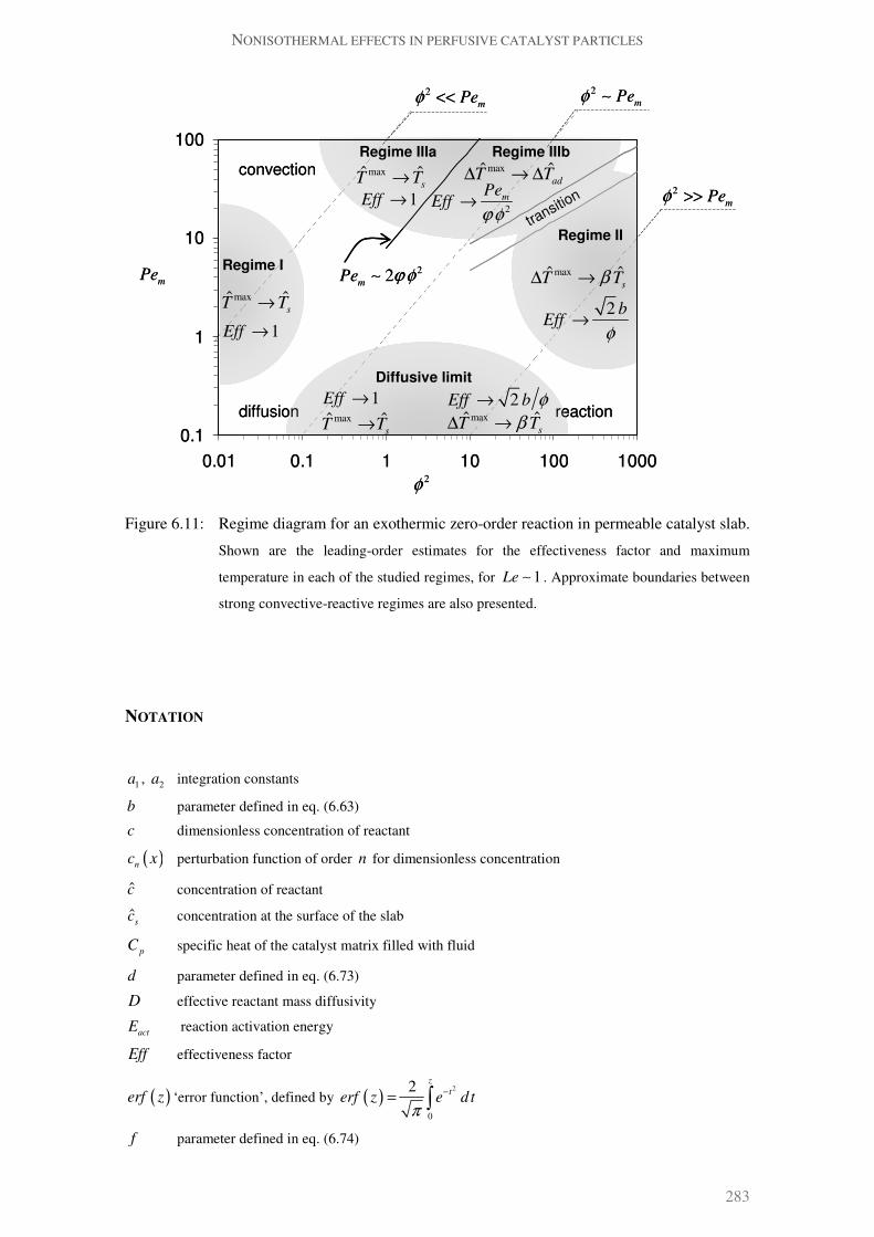
NONISOTHERMAL EFFECTS IN PERFUSIVE CATALYST PARTICLES
283
Figure 6.11: Regime diagram for an exothermic zero-order reaction in permeable catalyst slab.
Shown are the leading-order estimates for the effectiveness factor and maximum
temperature in each of the studied regimes, for 1Le ∼ . Approximate boundaries between
strong convective-reactive regimes are also presented.
NOTATION
1a , 2a integration constants
b parameter defined in eq. (6.63)
c dimensionless concentration of reactant
( )nc x perturbation function of order n for dimensionless concentration
c concentration of reactant
ˆs
c concentration at the surface of the slab
pC specific heat of the catalyst matrix filled with fluid
d parameter defined in eq. (6.73)
D effective reactant mass diffusivity
actE reaction activation energy
Eff effectiveness factor
( )erf z ‘error function’, defined by ( )2
0
2 z
terf z e d t
π
−= ∫
f parameter defined in eq. (6.74)
2m
Peφ ∼2
mPeφ <<
2m
Peφ >>
reactiondiffusion
convection
2φ
mPe
Diffusive limit
transitio
n
Regime IIIb
Regime I
Regime II
maxˆs
T T→
1Eff →
maxˆs
T Tβ∆ →
maxˆad
T T∆ → ∆maxˆs
T T→
1Eff →2
mPe
Effϕ φ
→
Regime IIIa
2 bEff
φ→
2Eff b φ→maxˆ
sT Tβ∆ →
1Eff →
maxˆs
T T→
22m
Pe ϕ φ∼
0.1
1
10
100
0.01 0.1 1 10 100 1000
2m
Peφ ∼2
mPeφ <<
2m
Peφ >>
reactiondiffusion
convection
2φ
mPe
Diffusive limit
transitio
n
Regime IIIb
Regime I
Regime II
maxˆs
T T→
1Eff →
maxˆs
T Tβ∆ →
maxˆad
T T∆ → ∆maxˆs
T T→
1Eff →2
mPe
Effϕ φ
→
Regime IIIa
2 bEff
φ→
2Eff b φ→maxˆ
sT Tβ∆ →
1Eff →
maxˆs
T T→
22m
Pe ϕ φ∼
0.1
1
10
100
0.01 0.1 1 10 100 1000
CHAPTER 6
284
( )H−∆ heat of the exothermic reaction
k intrinsic kinetic constant
sk kinetic rate constant evaluated at the surface temperature of the catalyst
L semi-thickness of the slab
Le Lewis’ number ( )Dκ=
hPe intraparticular heat Peclet number ( )u L κ=
mPe intraparticular mass Peclet number ( )u L D=
( )r T dimensionless reaction term
R ideal gas constant
T dimensionless temperature
( )nT x perturbation function of order n for dimensionless temperature
T temperature
sT temperature at the surface of the slab
T∆ characteristic temperature change
adT∆ adiabatic temperature change
difT∆ maximum temperature change observed in a diffusive-reactive system with
concentration annulment
u superficial fluid velocity
x dimensionless transverse position within the slab
x transverse position within the slab
'x position where concentration reaches annulment on the left side of the slab
*x position where concentration reaches annulment on the right side of the slab
xɶ point where outer solution takes zero concentration value
X stretched coordinate in the region near 1x =
*X stretched annulment position near 1x =
*n
X coefficients in the expansion for *X
Y stretched coordinate in the region near 1x = −
'Y stretched annulment position region near 1x = −
'n
Y coefficients in the expansion for 'Y
Greek letters
β Prater’s parameter ( ) ( )( )ˆˆs p s
H Dc C Tρ κ= −∆
δ thickness of the boundary layer
ε small (perturbation) parameter
φ Thiele modulus ( )( )ˆs s
L k c D=
( )2
critφ critical Thiele modulus value, above which concentration annulment occurs
γ Arrhenius parameter ( )( )ˆact s
E RT=

NONISOTHERMAL EFFECTS IN PERFUSIVE CATALYST PARTICLES
285
η characteristic temperature change normalized by surface temperature ( )ˆs
T T=∆
ϕ nonisothermal parameter ( )γ η=
κ fluid-filled catalyst effective thermal diffusivity ( )pCλ ρ=
λ effective thermal conductivity of the fluid-filled catalyst
ρ density of the catalyst matrix filled with fluid
Subscripts
max maximum
min minimum
n order of the perturbation function
Superscripts
comp composite
l left
m middle
max maximum
min minimum
r right
REFERENCES
Allen, J. W. and S. N. Bhatia (2003). "Formation of steady-state oxygen gradients in vitro: Application to liver zonation." Biotechnology and Bioengineering 82(3): 253-262.
Aris, R. (1975). The mathematical theory of diffusion and reaction in permeable catalysts. London, Oxford University Press.
Bender, C. M. and S. A. Orszag (1999). Advanced Mathematical Methods for Scientists and Engineers. New York, Springer-Verlag.
Cardoso, S. S. S. and A. E. Rodrigues (2006). "Diffusion and reaction in a porous catalyst slab: Perturbation solutions." AIChE Journal 52(11): 3924-3932.
Cardoso, S. S. S. and A. E. Rodrigues (2007). "Convection, diffusion and reaction in a nonisothermal, porous catalyst slab." AIChE Journal 53(5): 1325-1336.
Chung, C. A., C. W. Chen, C. P. Chen and C. S. Tseng (2007). "Enhancement of cell growth in tissue-engineering constructs under direct perfusion: Modeling and simulation." Biotechnology and Bioengineering 97(6): 1603-1616.
Coletti, F., S. Macchietto and N. Elvassore (2006). "Mathematical modeling of three-dimensional cell cultures in perfusion bioreactors." Industrial and Engineering Chemistry Research 45(24): 8158-8169.
Damkohler, G. (1943). "The excess temperature in contact grains." Zeitschrift Fur Physikalische Chemie-Leipzig 193(1/3): 16-28.
CHAPTER 6
286
Fassnacht, D. and R. Pörtner (1999). "Experimental and theoretical considerations on oxygen supply for animal cell growth in fixed-bed reactors." Journal of Biotechnology 72(3): 169-184.
Frank-Kamenetskii, D. A. (1955). Diffusion and Heat Exchange in Chemical Kinetics. Princeton, Princeton University Press.
Goldstein, A. S., T. M. Juarez, C. D. Helmke, M. C. Gustin and A. G. Mikos (2001). "Effect of convection on osteoblastic cell growth and function in biodegradable polymer foam scaffolds." Biomaterials 22(11): 1279-1288.
Hlavacek, V. and M. Marek (1967). "Modelling of Chemical Reactors .V. Heat and Mass Transfer within a Porous Catalyst Particle - Some Results of an Analysis for a Zeroth-Order Reaction." Collection of Czechoslovak Chemical Communications 32(11): 4004-4017.
Lin, C. C. and L. A. Segel (1988). Mathematics Applied to Deterministic Problems in the Natural Sciences, SIAM.
Lopes, J. C. B., M. M. Dias, V. G. Mata and A. E. Rodrigues (1995). "Flow field and non-isothermal effects on diffusion, convection, and reaction in permeable catalysts." Industrial and Engineering Chemistry Research 34(1): 148-157.
Marek, M. and V. Hlavacek (1968). "Modelling of Chemical Reactors .VI. Heat and Mass Transfer in a Porous Catalyst Particle; On the multiplicity of solutions for the case of an exothermic zeroth-order reaction." Collection of Czechoslovak Chemical Communications 33(2): 506-517.
Martin, Y. and P. Vermette (2005). "Bioreactors for tissue mass culture: Design, characterization, and recent advances." Biomaterials 26(35): 7481-7503.
Nir, A. and L. M. Pismen (1977). "Simultaneous intraparticle forced convection, diffusion and reaction in a porous catalyst." Chemical Engineering Science 32(1): 35-41.
Prater, C. D. (1958). "The temperature produced by heat of reaction in the interior of porous particles." Chemical engineering Science 8(3-4): 284-286.
Prince, C. L., V. Bringi and M. L. Shuler (1991). "Convective Mass Transfer in Large Porous Biocatalysts: Plant Organ Cultures." Biotechnology Progress 7(2): 195-199.
Process Systems Enterprise (2007). gPROMS. London.
Quinta Ferreira, R. M. (1988). Contribuição para o Estudo de Reactores Catalíticos de leito fixo. Efeito da convecção em catalisadores de poros largos e casos de catalisadores bidispersos. University of Porto. PhD Thesis.
Rodrigues, A., B. Ahn and A. Zoulalian (1982). "Intraparticle Forced Convection Effect in Catalyst Diffusivity Measurements and Reactor Design." AIChE Journal 28: 541-546.
Rodrigues, A. E. (1981). Scientific bases for the design of two-phase catalytic reactors. Multiphase Chemical Reactors - Design Methods. A. E. Rodrigues, J. M. Calo and N. H. Sweed. Rockville, M.D., NATO ASI Series E-52. 2: 65-133.
Rodrigues, A. E., J. M. Orfao and A. Zoulalian (1984). "Intraparticle convection, diffusion and zero order reaction in porous catalysts." Chemical Engineering Communications 27(5-6): 327-337.
Schlichting, H. (1979). Boundary-Layer Theory. New York, McGraw-Hill.
Stephanopoulos, G. and K. Tsiveriotis (1989). "Effect of intraparticle convection on nutrient transport in porous biological pellets." Chemical Engineering Science 44(9): 2031-2039.

NONISOTHERMAL EFFECTS IN PERFUSIVE CATALYST PARTICLES
287
Wheeler, A. (1951). "Reaction Rates and Selectivity in Catalyst Pores " Advances in Catalysis 3: 249-327.
Young, M. W. and R. C. Dean (1987). "Optimization of Mammalian-Cell Bioreactors." Bio-Technology 5(8): 835-837.

CHAPTER 6
288
289
CHAPTER
SEVEN
CONCLUSIONS AND PERSPECTIVES OF FUTURE WORK
7
This thesis proposes an analysis for some chemical engineering problems involving convection,
diffusion and reaction. These phenomena occur at several scales: from a pore in a perfusive
catalyst particle to a wall-coated channel in a microstructured reactor. Our approach was mainly
based on approximate analytical methods, whose results were compared to the ones obtained
from numerical simulation. Since neither numerical nor experimental work were considered in
detail, it seems adequate that suggestions for future research should refer exclusively to
developments accomplished by means of analytical techniques alone or in combination with
others. In this chapter, we divide our contribution into eight topics, summarize main
achievements and propose possible extensions in each.
7.1 FINITE REACTION RATES IN A WALL-COATED MICROCHANNEL REACTOR
Assuming that a reaction proceeds sufficiently fast in a coated microchannel, so that
concentration annulment prevails at most part of its surface, may not be reasonable in many
practical situations. This has been highlighted throughout the thesis. In Chapter 4, we have
stressed that several studies in the literature reported to have incorrectly assumed operation
under full mass transport control. We also derived boundaries for this regime, which placed the
conditions for wall concentration annulment in a region corresponding to high values of the
Damköhler number ( Da ). In fact for this to happen, highly active catalysts would be required,
or alternatively high operating temperatures, as shown in Chapter 5 (which can lead to a change
in the reaction mechanism or activation of homogeneous reactions). In analytical applications,
this may require immobilization of a large quantity of ligand to guarantee that binding rates are
sufficiently fast. In Chapter 1, we have mentioned a heuristic design rule: the microdevice

CHAPTER 7
290
should be dimensioned so that transport rates ‘match’ reaction kinetics, or so that the former are
not limiting (i.e. even faster than the latter). Therefore, in applications with miniaturized
systems (with the purpose of reducing mass transfer resistance), the case of finite reaction rates
compared to transport (i.e. finite Da ) is relevant and is also the generic solution of the linear
transport-reaction problem. Even when operation close to the asymptotes occurs, expressions
for slow and fast reaction rates with ( )O Da and ( )1O Da corrections improve the estimation
of conversion significantly.
In Chapter 2, we have proposed simplified models for conversion calculation under finite values
of Da in the two main mass transfer regimes. In the fully developed regime, conversion of
reactant depends on Da through two quantities (the first eigenvalue 1λ and the first weight
1w ). We have proposed correlations to describe the variation of both quantities with Da . Our
expressions were constructed from the correct asymptotic limits and shown to be reasonably
accurate. They were also simple enough to be included in other quantities (namely conversion)
and allowed for the effect of Da to be exhibited explicitly in appropriate limits. Moreover, the
parameters in these correlations are dependent on the flow profile and geometry, and can be
easily generalized for other channel cross-sectional shapes. This allows a direct comparison
between different cases. When the concentration profile is developing, empirical formulas were
also used to describe conversion according to Lévêque’s analysis (which assumes a
concentration boundary layer near the wall, in a planar channel with linear velocity profile) for
all values of Da . These were shown to be accurate even for ~ 1Da , and valid for
( )~ 10m
Peα > .
The description of conversion with these results was compared with the numerical solution of
the full problem and the following remarks can be made:
1. The accuracy of the fully developed regime decreases as expected with the magnitude of
Graetz parameter (especially for ~ 10m
Pe zα > ), but mainly for high values of Da ;
2. Curvature decreases the range of validity of the fully developed profile at high m
Pe zα ,
especially for large Da , identifying the need for an higher order correction;
3. The empirical correlations describing the leading-order Lévêque solution have
comparable or even better agreement with the numerical solution than the individual
limits at high and low Da , from which they were constructed;
4. An higher order perturbation correction to the developing profile solution due to
curvature in a channel with plug-flow is more important at high Da and can be written as
a sum of two parcels of order ( )mO z Peα and ( )( )m
O z Da Peα , where the latter
(subdominant) accounts for finite (large) reaction rates. In the opposite limit (low values
of Da ), the correction is ( )2
mO Da z Peα
, which is very small at the inlet;

CONCLUSIONS AND PERSPECTIVES OF FUTURE WORK
291
5. Nonlinearity of velocity profile near the wall in laminar flow has to be considered also at
high Da and terms with order ( )mO z Peα and ( )( )
2/32/3m
O z Da Peα
should be
added to the leading-order problem. At low Da , the correction is only of
( )5/32
mO Da z Peα
;
6. Correction due to curvature in developing profile is more important than the one due to
nonlinearities in the velocity profile, and both are more relevant for 1Da >> .
Additionally, it was exemplified how a channel can be dimensioned so that the required
conversion is attained and how the results presented in Chapter 2 can avoid simulations in large
parametric areas, or restrict the search for adequate design to particular configuration/operation
sets. In comparison with the numerical solution, this also allowed the decoupling of effects such
as geometry and flow profile.
7.1.1 Suggestions for future work
Extension of the work presented is possible for similar models to the one adopted, but
encompassing other effects which may be important at the microscale. We refer specifically to
viscous dissipation and simultaneous development of the velocity profile (Herwig 2008). In fact
recently, Gundlapally et al. (2011) have used very similar techniques to the ones presented in
Chapter 2 to predict the variation of Sherwood number with Graetz and Schmidt’s numbers.
They however considered uniform wall concentration and flux boundary conditions. It is
possible that the effect of a reaction occurring at the wall may be superposed on these
dependences and yield a more generic solution. In the case where flow is allowed to develop
over the same distance of the concentration profile it would be interesting to evaluate how
conversion is affected with Schmidt’s number, namely if it changes from the plug-flow
asymptote to the laminar flow one, and estimate the error introduced by taking these limiting
models for channel flow. Concerning the effect of viscous dissipation, a great deal of work
already exists, but it is mainly focused on the heat transfer problem and not in the nonisothermal
reactive case (Aydin 2005; Morini 2005; Aydin et al. 2006; Barletta et al. 2006; Jeong et al.
2006; Magyari et al. 2006; Chiba et al. 2008).

CHAPTER 7
292
7.2 APPROXIMATE SOLUTIONS FOR NONLINEAR KINETICS
There are not many available analytical treatments for the case of nonlinear wall kinetics. The
most used strategies were reviewed in Chapter 2, but even the ones with a strong analytical
character end up having to be evaluated numerically. With today’s computational capabilities
this actually makes the problem solution less straightforward than simply solving numerically
the governing equations with appropriate boundary conditions.
In our work in Chapter 2, we have proposed a perturbation procedure to obtain analytical,
explicit expressions for conversion as a function of the reaction order m in the case of a power-
law kinetics. However, this introduced a limitation: intermediate values of Da may be
satisfactorily approximated (and this indeed happens in some cases) but this is not guaranteed
by the method, which predicts higher errors as Da increases/decreases from zero/infinity. This
happens because the solutions were constructed from two limits associated with Da , which is
the only parameter appearing next to the ‘problematic’ concentration nonlinear term in the
kinetic law. Moreover, we have considered also the two main mass transfer regimes (developing
and fully developed) to solve the mass balance in the simplest way possible. Nevertheless, it
was possible to achieve some insight concerning the effect of the reaction rate law in
conversion, namely:
1. The form of the perturbation expansion for mixing-cup concentration is different in the
kinetic and in the mass transfer controlled limits: while in the former, the influence of m
appears implicitly in the coefficients that are calculated; in the later there is also the
explicit appearance of m in the order of the gauge functions of the perturbation
parameter, which constitutes the expansion ( /
0
n m
n
n
c c ε
=
=∑ ).
2. For orders of reaction 1m > , the results for conversion normalize with the kinetic control
asymptote up to higher values of Da . On the other hand for 1m < , deviation from the
leading-order solution is negligible for small Da but gets more pronounced as the value
of this parameter increases.
3. For orders of reaction 1m < , the orders of subsequent corrections to the Dirichlet leading-
order term are much lower in magnitude ( ( )/n m
O ε ), which means that the deviation from
the full mass transfer control decreases sharply as 0ε → (i.e. better agreement with the
Dirichlet limit for the same Da is observed).
4. Perturbation corrections are especially required when 1m > in the mass transfer
controlled regime, and in the kinetically controlled regime when 1m < .
CONCLUSIONS AND PERSPECTIVES OF FUTURE WORK
293
5. In the determination of intrinsic reaction rate parameters, reactions orders with 1m < are
expected to deviate the most from the normalization if low Da conditions cannot be
assured.
6. When mass transfer controlled conditions are attained numerical integration may present
some increased difficulties (e.g. when concentration near the wall oscillates to zero and
the wall reaction is of ‘power law’ type with non-integer exponent; or when boundary
layers near the wall exist). Therefore, analytical results are particularly convenient in this
case.
7. The changes in behavior for 1m < and 1m > are related to kinetic / mass transfer control
and the same trends were observed in the fully developed and developing limits. In the
case of developing profile, the perturbation parameter was the rescaled Damköhler
number detailed in Chapter 4. In this case, even though corrections due to curvature and
velocity profile nonlinearities in a circular channel with laminar flow are important ( as
seen in section 2.3), accounting for the order of reaction reduces errors by one order of
magnitude (e.g. for * 0.1Da = and 100m
Peα = , the maximum deviation for 2m = is
0.06%). Nevertheless, we note that the leading-order extended corrections from section
2.3 (accounting for curvature and nonlinear flow profile) are valid in these limiting cases
too and can be added.
7.2.1 Suggestions for future work
Further analytical treatment on the effect of nonlinear reaction rates or more complex kinetics is
likely to be more limited and demanding of numerical evaluation. However, the limiting
solutions can be used in semi-numerical procedures suggesting a dependence of conversion on
the governing parameters. For example, Spence et al. (1995) has noted the difficulties in the
numerical solution of a one-dimensional model for power-law kinetics with non-integer reaction
exponent m , when concentrations reach zero at the wall. To overcome this problem, an
exponential substitution for the wall concentration is suggested, which helps the numerical
evaluation if a coefficient in the argument of the exponential is set to 1000. This fitting relates
directly to our analysis in section 2.4.2a. It is possible that our results can be used to improve
numerical evaluation, based on a theoretical analysis and without the need for fitting
coefficients. It would also be interesting to evaluate how the results presented can be employed
in the determination of intrinsic kinetic parameters and rate expressions, and how available
kinetics (determined from other methods) compare with these solutions.

CHAPTER 7
294
7.3 UNIFORMLY VALID SOLUTION TO GRAETZ’S PROBLEM
We have pointed out that most literature analyzes transport-reaction problems in microchannels
in one of two main mass (or heat) transfer regimes. We have also done so in Chapter 2, even
though corrections to Lévêque’s leading-order result were proposed to extend its validity to
lower values of Graetz’s parameter (m
Pe zα ), for finite reaction rates. In Chapter 3, we
reviewed several attempts to analytically describe the two simplified regimes in a single
uniformly valid composite solution and have concluded that the existing approaches were
unsatisfactory. Therefore, based on a feature of the eigenvalues on the exact solution, we
propose the application of an asymptotic technique to obtain a general solution for concentration
conversion (temperature change). Furthermore, we have identified in the obtained result the
contributions of the fully developed and developing limits and two correcting functions
accounting for the importance of each one in the composite solution. The overall quantity χ ,
which may be conversion of reactant R
X by an infinitely fast reaction (or also when kinetics is
moderately fast but finite, 1Da > ) or the reciprocal of Sherwood number in Neumann boundary
condition (1 Sh ), writes as:
fd fd dev devχ χ χ= Θ + Θ (7.1)
where fd
χ is the value of χ in the fully developed regime (associated with the first term in an
series of eigenfunctions), dev
χ is the solution when the concentration/temperature profile is
considered only in a boundary layer near the wall. Moreover, fd
Θ is a function depending on
the coefficients from the first term in Graetz series and accounts for the other terms that are not
being retained in the fully developed limit. On the other hand, dev
Θ has the form of an
incomplete Gamma function, whose arguments include the Graetz parameter and quantities
depending on the shape of the channel, the flow profile and the boundary layer thickness.
The solutions of the form of (7.1) fulfill both limiting solutions and also yield very acceptable
results in the transition regime, as it was shown for the channel geometries, flow profiles and
boundary conditions studied in Chapter 3. No numerical evaluation is required and higher order
terms don’t need to be considered. The abundant information concerning the first term in Graetz
series can be used to construct an uniform solution, with no additional information required.
The same procedure was applied to the case of finite wall resistance (due to a finite reaction or
nonzero thermal resistance). We believe that the combination of limiting models for heat/mass
transfer in (7.1) is particularly important at the microscale, where both regimes can be found
(millisecond contact times locate the operation at the inlet regime or at least a non-negligible
entrance length inside the channel exists). It is also possible that, depending on the objective
function for performance adopted in a particular application, the optimum operation is in the
CONCLUSIONS AND PERSPECTIVES OF FUTURE WORK
295
transition region between the two models, which can be conveniently represented by our
analytical solution.
7.3.1 Suggestions for future work
(Graetz 1883)
The Graetz problem is a classic one (the original solution by Graetz goes back to 1883), it is
very fundamental in mass/heat transfer theory (Shah et al. 1978) and has been object of many
modifications/extensions which are often referred as Graetz solutions (Weigand et al. 2007;
Cossali 2009; Haji-Sheikh et al. 2009; Haji-Sheikh et al. 2010; Ray et al. 2010). The same
comments apply to Lévêque’s analysis (1928), and generalized Lévêque-type solutions are also
present in the literature (Vera et al. 2011). Recently, these problems have gained an additional
source of interest in the context of microchannel heat exchangers/reactors, for which a
considerable number of studies are currently being published. We note that several reviews have
reported that conventional macroscale theory is able to describe channel phenomena in the
dimensions considered here, as long as microscale effects are considered. Inlet
concentration/temperature boundary layers are one of these effects. Despite the fact that these
problems constitute the basis of analysis of many diverse phenomena, the analytical treatment is
generally the same (yielding an infinite series). This is a common characteristic shared with
other linear partial differential equations, whose particular solutions are combined by the
principle of superposition.
From the examples presented in this thesis, we believe that the application of asymptotic
summation of series techniques (in particular, of the Euler-Maclaurin formula) may be of
interest for a number of cases currently discussed in the literature. We note that this approach
allows us to simultaneously obtain the corresponding Lévêque-type solution or correction, as
this is a natural outcome of the procedure. Examples of possible extensions in the channel
transport context include conjugate problems in heat transfer (Papoutsakis et al. 1981a;
Papoutsakis et al. 1981b), axial diffusion effects (Acrivos 1980; Papoutsakis et al. 1980b;
Papoutsakis et al. 1980a; Haji-Sheikh et al. 2009) and viscous dissipation (Aydin et al. 2010),
among others. In particular, we propose three suggestions:
1. Considering axial diffusion in the problem, yields solutions with the same form of the
problem considered in Chapter 3, but with coefficients which exhibit a more complex
dependence on the governing parameters. However, it is possible to anticipate that by
expansion of functions for plug-flow and WKB methods for laminar flow, the asymptotic
behavior of these quantities can be obtained. For example, for Dirichlet boundary
conditions with plug-flow between parallel plates,

CHAPTER 7
296
( )3
2 2 2 31 2
~8
m
n n m
PePe O n
nλ λ λ π
π
−
+∆ = − − +
In this case, the spacing between eigenvalues also depends on the transverse Peclet
number. At this stage, we recall the usefulness of empirical correlations to translate the
parametric dependence of these quantities in a simple, but accurate manner. Then, with
some additional assumptions the Euler-Maclaurin sum formula may still be an excellent
tool to obtain a complete solution, with the advantages mentioned above. This results in
an analysis which may be uniform in 2α and
mPeα . Therefore, for channels without
small aspect ratios general solutions can be obtained.
2. For the case of simultaneous development of the velocity profile, although the
coefficients that appear in that case are also functions of other parameters, it would be
interesting to understand if the same method applies.
3. In the case of a simultaneous homogeneous reaction (which may be activated at higher
temperatures), the form of the solution is similar, but with coefficients that also depend
on the bulk Damköhler number (defined with the homogeneous reaction rate at reference
conditions). Developments in this problem may be expected.
7.4 DEGREE OF PROFILE DEVELOPMENT
One of the consequences of deriving a solution valid in all points of the domain and parametric
space that we found particularly interesting was the estimation of boundaries for application of
the well-known limiting solutions. This has been translated in the literature through several
related quantities, e.g.: entrance length, incremental heat transfer number, thickness of boundary
layer,... and has been determined in a number of ways, detailed in Chapter 3. Most of them are
not explicit in the criterion, which at some point will have to be set arbitrarily. In our work, we
have defined a degree of transverse control which measures the agreement with the fully
developed asymptote. We concluded that the results were more insensitive to the formulated
criterion in the fully developed boundary, whereas the inlet region depends more expressively
on the level of agreement required with Lévêque’s solution. Also, in the fully developed
boundary the effect of flow profile is negligible. The transition region may occupy a large part
of the channel domain. This can also be related with the pressure drop experienced in the system
and the level of influence of inlet effects (which increase mass transfer) present in the system. In
the case of a finite reaction rate, we have observed that for 1Da > , the entrance length is near
the fast reaction asymptote, while for 0Da → the applicability of the 1-term Graetz solution
increases up to the inlet.

CONCLUSIONS AND PERSPECTIVES OF FUTURE WORK
297
7.4.1 Suggestions for future work
We have suggested that the uniformly valid solutions obtained in section 7.3.1 could be useful
to analyze other problems. The definitions of transition boundaries would follow in the same
terms. One adaptation of our results which would probably not require much additional effort is
based on the idea behind one of the methods that are used for estimating the concentration
profile length: analogy with the development of the velocity profile. This leads to the
substitution of Reynolds number by Peclet number (i.e. multiplication by the Schmidt number)
with negligible alteration of the numerical coefficients. Therefore the development of the
velocity profile alone in a duct (with the shape normalization possibility pointed out in
Chapter 3) could be treated in the same way. The effect of the simultaneous velocity and
concentration/temperature development on these boundaries it is also of interest. Our ideas can
be extended to a number of other cases. In particular and to highlight the effects of the
microscale on the fluid dynamics, the results for finite wall resistance (finite Da) can share some
similarities with the case of developing velocity slip (flow) in a channel with isothermal wall.
7.5 MAPPING OF OPERATING REGIMES AND THE CONCEPT OF “RESCALED
DAMKÖHLER NUMBER”
In the previously identified contributions, the regimes proposed by the analysis were mainly
concerned with the interaction of convection through the channel (in streamlines parallel to the
surface defined by the wall) and transverse diffusion towards the catalyst coating. We proceeded
to also incorporate the coupling of these transport mechanisms with the magnitude of reaction
rate occurring at the channel wall. This was done in two parts. First, we focused on the external
mass transport effects on a surface reaction in Chapter 4 (with internal phenomena lumped in
the effectiveness factor). Then, the internal phenomena (at the catalytic coating level) was
considered in more detail in Chapter 5.
Concerning the definition of external kinetically controlled and mass transfer controlled regimes
the following was achieved (Chapter 4):
1. We have defined in line with what has been presented in the literature, a degree of mass
transfer control θ , which is a concentration ratio;
2. Explicit expressions for θ were presented in the fully developed and developing limits
for kinetic and mass transfer controlled regimes;
3. In each limit of the convection-transverse diffusion balance, correlations for θ were
proposed to describe all values of Da ;
CHAPTER 7
298
4. Criteria for kinetic and mass transfer control valid for all values of the Graetz parameter
and of the form ( ),m
Da Da Pe zθ α= were proposed and describe very reasonably the
results obtained from numerical simulations with gPROMS®;
5. Iso-θ curves were plotted in a m
Da Pe zα− diagram, in particular for specified low and
high specified values of θ (kinetic and mass transfer control, respectively);
6. The achievement of external mass transfer control required high values of Da , even for
low m
Pe zα . Moreover, the effect of increasing the Graetz number is visible by
demanding more severe conditions (translated e.g. into higher operating temperatures) to
attain the same degree of mass transfer control observed in the fully developed regime,
and
7. Previous criteria presented in the literature for specific values of θ (or related quantities)
can be incorporated in our analysis and they all prove to be in agreement with our results,
but are more limited or of less convenient evaluation.
The basis for defining these operating regimes has been the magnitude of the Damköhler
number. In our opinion, this has happened for several reasons: this was how the very influential
original work from Damköhler (1937) presented the problem; in many cases the effect of the
entrance length is still not considered and in these conditions the degree of mass transfer control
is indeed only a function of Da; simple magnitude relationships are attractive for the
interpretation of experimental work; and from analogy with other problems such as the internal
diffusion-reaction analysis based on the magnitude of Thiele modulus. However, we have seen
that the entrance length needs to be accounted for in microchannels and has influence on mass
transfer. Since this is an important parameter, we propose a modification based on the correct
scaling of the wall boundary condition,
*Da Da δ= (7.2)
where δ is the normalized thickness over which concentration decays in the channel. Most
literature consider ~ 1δ (i.e. the scale for concentration change in the channel is e.g. the
channel radius or the half spacing between parallel plates). However, we have shown that at the
convection-dominated (Lévêque’s) regime, this scale is not appropriate and the correct one
should be applied in (7.2). In this case, the limiting conditions for absence of radial
concentration gradients and wall concentration annulment are observed for * 0Da → and
*Da → ∞ , and this is more rigorous than taking the 0Da → and Da → ∞ limits. The
parameter in (7.2) was named as the ‘rescaled Damköhler number’ and the variation of θ with
*Da in the developing profile limit is similar to the ( )Daθ dependence on the fully developed
profile asymptote. We have also shown that the concept can be applied when the thickness over
which concentration changes is known as a result of other inner descriptions, incorporating
different mechanisms (namely axial diffusion at the inlet, section 4.5). In this case,
CONCLUSIONS AND PERSPECTIVES OF FUTURE WORK
299
concentration annulment at the wall near the inlet is also observed for high rescaled Damköhler
number, and the iso- *Da lines can also be plotted in a m
Da Peα− diagram, so that the regions
of influence of this effect are easily identified. Naturally, more severe conditions are required
for concentration annulment to occur at the inlet, and in this case the remaining portion of the
channel is also under full mass transfer control.
In Chapter 5, the interplay of these ‘external’ regimes with what is occurring inside the coating
was considered. In particular, we showed that internal limitations may be controlling in the
definition of a global (channel and washcoat) kinetic regime. This depends on the magnitude of
a parameter involving bulk and catalyst diffusivities as well as the ratio between the length
scales for diffusion at the channel and washcoat. It also explains why some studies observe
internal limitations in the absence of external ones in the same ranges of temperature that others
observe the opposite picture. Moreover, we have identified how the parameters relate to each
other in the transition between regime definition from internal and external phenomena, which
apart from geometrical and kinetic-related quantities is given by
eff eff
w m
D D
D Sh t kε= ,
where m
k is the mass transfer coefficient, eff
D the effective diffusivity in a coating with
thickness w
t .
The boundaries were plotted in terms of the operating variable of interest, in this case
temperature, as a function of a dimensionless parameter. However, this is just done for
convenience since this dimensionless variable can be converted to a geometric feature of the
design, if other quantities are kept fixed. Several expressions for the limiting temperatures
which bound different regimes were proposed and are of convenient evaluation. These results
make use of two quantities that can be set by the user as desired: the degree of mass transfer
control θ (defined in Chapter 4) and the effectiveness factor (for which approximations in
Chapter 5 were provided), which express the mass transfer resistances in the channel and
coating, respectively.
7.5.1 Suggestions for future work
As mentioned in Chapter 1, microdevices open the possibility of operating in new parametric
windows. It would be interesting to identify some of those regions in the constructed parametric
map, once more information concerning production-scale technologies becomes available. On
the other hand, it would also be of interest to draw the path of the chain of process development
CHAPTER 7
300
in the proposed regime diagram: from kinetic studies (at low Da) to chemical production at
different scales.
In the case of axial diffusion being also considered in the analysis of the extended Graetz
problem, a third axis should be added to the diagram, corresponding to the aspect ratio (which
governs the magnitude of axial diffusion effects to the transverse diffusion one). The case of
nonisothermal systems would also add at least two parameters (concerning heat generation and
conduction), assuming that others such as Arrhenius number with activation energy are kept
fixed. The influence of inlet effects (in the sense detailed in section 4.5) should be also relevant
in the investigation of local effects in fast reactions and ignited states. The results of our
simplified new description for the boundary layer could be pursued in this context.
7.6 EVALUATION OF THE EFFECTIVENESS FACTOR IN A THIN CATALYST COATING
In the previous topics, external transport (in the channel) and its interaction with reaction were
discussed while effects at the catalyst coating level were lumped by an effectiveness factor (η )
and incorporated into the Damköhler number. As in most literature, we adopt the effectiveness
factor concept as the basis for the analysis of the internal transport-reaction competition. Other
related quantities (concentration ratios, linear driving force coefficients, mass transfer
coefficients) imply a linearization of the concentration profile near the wall and in terms of
evaluation are of comparable difficulty. Concerning our approach for the calculation of η , the
main achievements in Chapter 5 were:
1. We wrote a reduced order model to represent reaction and diffusion in a catalytic coating
with arbitrary shape. The general 3D equations were reduced to a 2D model by making
use of a transformation to the curvilinear orthogonal coordinate system, as described
elsewhere (Datta et al. 1985; Mariani et al. 2003). The resulting mass balance is further
simplified by applying a perturbation method for thin coatings, reducing the problem to a
1D domain.
2. The concentration profile inside the catalytic coating (normalized by its value at the
surface) depends on the following parameters: Thiele modulus 2φ (defined with the
characteristic length for diffusion, i.e. the maximum distance in the direction normal to
the fluid-solid interface); the ratio of length scales for diffusion in the coating and in the
channel (ε ); and the ratio of washcoat volume to interfacial area and to the internal
diffusion length scale (υ ).
3. The concentration distribution and the effectiveness factor can be written as a series in
powers of ε , assuming small values of this parameter. We consider the first two terms in

CONCLUSIONS AND PERSPECTIVES OF FUTURE WORK
301
this expansion. This has proven to be reasonable in some cases even for ( )~ 1Oε . Note
that considering more terms in the perturbation series may improve the approximation
near 0ε = , but may cause serious divergence as ε increases. Therefore, our two-term
solution is appropriate.
4. The obtained result for η can be written in terms of the aforementioned geometry-related
parameter (υ ) and of the effectiveness factor for an equivalent slab (slab
η with the same
length scale for diffusion). This was shown to be rigorously true in the case of
perturbation solutions with linear kinetics (valid for all values of 2φ ) and arbitrary
geometry (as long as 1ε < ). Nevertheless, reasonable agreement with numerical solutions
is obtained even for ~ 1ε .
5. Based on the analysis for high and low 2φ , we speculated that the previous expression for
η would also apply to the case of a reaction rate expression with arbitrary form. This was
confirmed by comparison with the numerical solution for several ‘normal’ kinetics. In
this case, the evaluation of slab
η has to be done for the particular reaction law. An
approximate procedure for this was proposed, which is based on the solution for linear
kinetics with a modified Thiele modulus 2Φ , including the classical normalization at high
reaction rates and the correct behavior in the chemical regime.
6. The same result was also shown to improve the calculation of η in nonuniform
geometries. Namely, by introducing a correction to the ‘slice method’ from Papadias et
al. (2000), the error associated with this approximation decreases, especially in the
intermediate region of 2φ .
7. The analysis was also applied to thin catalytic coatings supported on impermeable/inert
particles to model egg-shell catalysts. It was found that the same expression was valid not
only for uniform surface concentration conditions, but also when external mass transfer
resistance was present.
7.6.1 Suggestions for future work
It would be interesting to further extend the perturbation techniques here employed to the cases
where angular diffusion needs to be considered. This would allow a better description of
nonuniform coatings and eventually provide analytical expressions for the local differential
effectiveness factor, as defined by Hayes et al. (2005). This also relates to the more general case
of a reaction-diffusion problem in a nonuniform geometry with peripheral variation of surface
concentration (which is likely to be found in irregularly coated channels). The suitability of our
approximation for η in the case of abnormal kinetics or with solution multiplicity also deserves
CHAPTER 7
302
further investigation. However, since these effects usually manifest themselves in an
intermediate range of the Thiele modulus, it is possible that the corrections in the chemical and
diffusional limits can still be applicable. Other natural extensions of this work would include
nonisothermal systems and systems with multiple reactions (for which the validity of the one-
dimensional cylindrical model was already discussed in Keegan et al. (2005)). Taking into
account the good description of the finite mass transfer resistance case in egg-shell catalyst
particles, it can also be suggested that global effectiveness factors in a microchannel geometry
should be considered.
Solutions based on the ‘thin layer’ assumption and consequent perturbation corrections should
be useful to a number of other systems, e.g. related with pellicular adsorbents. Specific
problems may include the measurement of diffusivities from chromatographic methods (where
the effectiveness factor in the steady-state problem is related to the transfer function in
Laplace’s domain of the transient non-reactive problem). Multilayer egg-shell particles (catalyst
or adsorbents) could benefit from this approach as well, even if the solution also requires some
numerical evaluation.
7.7 PERFUSIVE COATINGS AND MONOLITHS
The second main direction for process intensification we have focused on is the improvement of
mass transfer by promotion of an additional transport mechanism in porous catalytic bodies:
intraparticular forced convection. In Chapter 5, we have applied a perturbation method
conceived for thin coatings to a permeable curved wall, which can be the surface of a perfusive
monolith for example. We developed an approximation for the effectiveness factor for this case,
which described correctly the numerically obtained solution, for several values of the
intraparticular Peclet number P , Thiele modulus 2φ , ratio of surface concentrations 2c , and
channel/coating diffusion length scales ratio ε (including ε near 1).
We then examined a regime described by dominance of intraparticular convection and reaction,
where we have found the most expressive enhancement of the effectiveness factor compared to
a nonpermeable (negligible convection) catalyst in the same conditions. The combination of
parameters at which the improvement was maximum was derived explicitly. This was found to
be an increasing function of P , but reaction rate should also ‘match’ with the increased
transport rates, according to 2 ~ Pφ .
CONCLUSIONS AND PERSPECTIVES OF FUTURE WORK
303
7.7.1 Suggestions for future work
In this case, we believe that considering external mass transfer will lead to much more
complicated analytical expressions, and one can doubt of its usefulness. Nevertheless, some
progress may occur with the simplified analysis in section 5.7.3.
It would be perhaps more interesting to incorporate our results at the single channel level into
the (probably numerical) solution of more complex systems. This may appear e.g. in a specified
arrangement of channels, where interaction between them happens due to suction/injection
through the wall.
7.8 MAXIMUM TEMPERATURE RISE IN PERFUSIVE CATALYST PARTICLES
We continued to explore the effects of intraparticular convection on the behavior of catalytic
porous solids in Chapter 6. In this case, the problem of an exothermic reaction in a slab-shaped
catalyst particle was considered. This added transport and generation of heat to the mass
transfer-reaction interaction. We conducted a scaling analysis to reach the following
conclusions:
1. According to the mass balance, three dominant regimes can be identified. Each one
reflects a balance between two mechanisms (convection, diffusion and reaction). These
are related with the limiting regimes defined from the energy balance by assuming an
order of magnitude for Lewis number.
2. The scale for temperature change T∆ due to the occurrence of an exothermic reaction is
predicted in several areas of the 3D parametric diagram formed by Thiele modulus,
intraparticular mass Peclet number and Lewis number.
3. Different behaviors concerning T∆ were observed, namely: isothermal (where
temperature rise is negligible); diffusive (where Prater’s relationship (Prater 1958) for
non-permeable catalyst holds); adiabatic (where the adiabatic temperature rise is
observed); and ‘explosion’ (where concentration annulment occurs and rescaling is
required).
A perturbation analysis was then applied to the three main operating regimes to estimate
concentration and temperature profiles, effectiveness factor and maximum temperature attained
inside the catalyst. In particular, we note that
1. In the transport dominated case (chemical regime), a regular perturbation expansion
expressed the small deviation of concentration and temperature from their surface values.
CHAPTER 7
304
2. In the diffusional regime, concentration (and temperature) variation only occurs at thin
boundary layers near the surface, where reaction dominates with diffusion (the core of the
catalyst is free from reactant). The effect of convective transport in these regions is of the
order of m
Pe φ . This is also the order of the correction to Prater’s limit (Prater 1958) in
the maximum temperature estimate.
3. In the limit of strong convection, two distinct situations are considered depending on
whether concentration annulment occurs or not. In the latter case, the problem is
described at most part of the domain (starting from the inlet) by a smooth variation of
concentration/temperature. Then, near the ‘exit’ of the slab (downstream) a relatively
sharper decrease from surface values may be observed (in a region with thickness
1m
Pe ). However, maximum concentration and temperature changes are small.
4. When concentration reaches annulment in a ‘dead core’ inside the slab, we consider the
same structure for the boundary layer near the exit of the slab, but matched with the
annulment branch of the solution. A boundary separating this regime from the diffusional
one was provided. The transition between convection dominated regimes (with and
without annulment) was also estimated analytically.
5. When convection is strong, but reaction is also fast enough to cause some annulment in
the reactant’s concentration, maximum effectiveness factor and temperature change are
observed. Namely, the adiabatic temperature rise is obtained at leading-order and the
effectiveness factor presents a very similar dependence to the optimum enhancement
conditions in Chapter 5, with a contribution accounting for nonisothermal behavior (both
analyses refer to the convection-reaction dominant balance).
The adiabatic temperature limit is frequently found as the maximum temperature in systems
with coupled processes. For example, in the case of premixed flames from combustion theory
(Law 2006). The same result was also found in catalyst particles with negligible intraparticular
convection. Belfiore (2007a; 2007b) considered strongly exothermic reactions (Prater’s
parameter, 1β → ) with Dufour and Soret effects, and temperature dependence of
physicochemical properties. The adiabatic temperature rise was found and named as a
‘generalized Prater equation’.
7.8.1 Suggestions for future work
Extensions of this topic may include examination of other catalyst geometries. It could also be
interesting to evaluate how kinetic normalization (e.g. the generalized Thiele modulus defined
in Chapter 5) applies in the presence of internal convection. The effect of finite mass/heat
CONCLUSIONS AND PERSPECTIVES OF FUTURE WORK
305
resistance and analytical bounds for the range where steady-state multiplicity occurs are also
possible topics for future research.
REFERENCES
Acrivos, A. (1980). "The extended Graetz problem at low Peclet numbers." Applied Scientific Research 36(1): 35-40.
Aydin, O. (2005). "Effects of viscous dissipation on the heat transfer in a forced pipe flow. Part 2: Thermally developing flow." Energy Conversion and Management 46(18-19): 3091-3102.
Aydin, O. and M. Avci (2006). "Viscous-dissipation effects on the heat transfer in a Poiseuille flow." Applied Energy 83(5): 495-512.
Aydin, O. and M. Avci (2010). "On the constant wall temperature boundary condition in internal convection heat transfer studies including viscous dissipation." International Communications in Heat and Mass Transfer 37(5): 535-539.
Barletta, A. and E. Magyari (2006). "Thermal entrance heat transfer of an adiabatically prepared fluid with viscous dissipation in a tube with isothermal wall." Journal of Heat Transfer 128(11): 1185-1193.
Belfiore, L. A. (2007a). "Effects of the collision integral, thermal diffusion, and the Prater number on maximum temperature in macroporous catalysts with exothermic chemical reaction in the diffusion-controlled regime." Chemical Engineering Science 62(3): 655-665.
Belfiore, L. A. (2007b). "Soret diffusion and non-ideal dufour conduction in macroporous catalysts with exothermic chemical reaction at large intrapellet Damköhler numbers." Canadian Journal of Chemical Engineering 85(3): 268-279.
Chiba, R., M. Izumi and Y. Sugano (2008). "An analytical solution to non-axisymmetric heat transfer with viscous dissipation for non-Newtonian fluids in laminar forced flow." Archive of Applied Mechanics 78(1): 61-74.
Cossali, G. E. (2009). "Analytical solution of Graetz problem in pipe flow with periodic inlet temperature variation." International Journal of Heat and Mass Transfer 52(13-14): 3396-3401.
Damköhler, G. (1937). "Einfluss von Diffusion, Strömung, und Wärmetransport auf die Ausbeute in Chemisch-Technischen Reaktionen." Chem.-Eng.-Tech 3(Part 1, Chapter 2): 359-485.
Datta, R. and S. W. K. Leung (1985). "Shape generalized isothermal effectiveness factor for first-order kinetics." Chemical Engineering Communications 39(1): 155 - 173.
Graetz, L. (1883). "Ueber die Wärmeleitungsfähigkeit von Flüssigkeiten." Annalen der Physik und Chemie 18: 79-94.
Gundlapally, S. R. and V. Balakotaiah (2011). "Heat and mass transfer correlations and bifurcation analysis of catalytic monoliths with developing flows." Chemical Engineering Science 66(9): 1879-1892.
Haji-Sheikh, A., J. V. Beck and D. E. Amos (2009). "Axial heat conduction effects in the entrance region of circular ducts." Heat and Mass Transfer/Waerme- und Stoffuebertragung 45(3): 331-341.

CHAPTER 7
306
Haji-Sheikh, A., W. J. Minkowycz and S. Manafzadeh (2010). "Axial conduction effect in flow through circular porous passages with prescribed wall heat flux." Heat and Mass Transfer/Waerme- und Stoffuebertragung 46(7): 727-738.
Hayes, R. E., B. Liu and M. Votsmeier (2005). "Calculating effectiveness factors in non-uniform washcoat shapes." Chemical Engineering Science 60(7): 2037-2050.
Herwig, H. (2008). Momentum and Heat Transfer in Microsized Devices. Micro Process Engineering: Fundamentals, Devices, Fabrication, and Applications. N. Kockmann. Weinheim, Germany, Wiley-VCH Verlag GmbH: 47-70.
Jeong, H. E. and J. T. Jeong (2006). "Extended graetz problem including axial conduction and viscous dissipation in microtube." Journal of Mechanical Science and Technology 20(1): 158-166.
Keegan, S. D., N. J. Mariani, O. M. Martínez and G. F. Barreto (2005). "Behaviour of smooth catalysts at high reaction rates." Chemical Engineering Journal 110(1-3): 41-56.
Law, C. K. (2006). Combustion Physics. New York, Cambridge University Press.
Lévêque, M. A. (1928). "Les lois de la transmission de chaleur par convection." Ann. Mines 13: 201-299.
Magyari, E. and A. Barletta (2006). "Thermally developing Poiseuille flow with a non-uniform entrance temperature when the viscous heat generation is significant." Journal of Physics A: Mathematical and General 39(14): 3829-3845.
Mariani, N. J., S. D. Keegan, O. M. Martínez and G. F. Barreto (2003). "A one-dimensional equivalent model to evaluate overall reaction rates in catalytic pellets." Chemical Engineering Research and Design 81(8): 1033-1042.
Morini, G. L. (2005). "Viscous heating in liquid flows in micro-channels." International Journal of Heat and Mass Transfer 48(17): 3637-3647.
Papadias, D., L. Edsberg and P. Björnbom (2000). "Simplified method for effectiveness factor calculations in irregular geometries of washcoats." Chemical Engineering Science 55(8): 1447-1459.
Papoutsakis, E. and D. Ramkrishna (1981a). "Conjugated Graetz problems-I. General formalism and a class of solid-fluid problems." Chemical Engineering Science 36(8): 1381-1391.
Papoutsakis, E. and D. Ramkrishna (1981b). "Conjugated Graetz problems-II. Fluid-fluid problems." Chemical Engineering Science 36(8): 1393-1399.
Papoutsakis, E., D. Ramkrishna and H. C. Lim (1980a). "The extended Graetz problem with Dirichlet wall boundary conditions." Applied Scientific Research 36(1): 13-34.
Papoutsakis, E., D. Ramkrishna and H. C. Lim (1980b). "Extended Graetz problem with prescribed wall flux." AIChE Journal 26(5): 779-787.
Prater, C. D. (1958). "The temperature produced by heat of reaction in the interior of porous particles." Chemical engineering Science 8(3-4): 284-286.
Ray, S. and D. Misra (2010). "Laminar fully developed flow through square and equilateral triangular ducts with rounded corners subjected to H1 and H2 boundary conditions." International Journal of Thermal Sciences 49(9): 1763-1775.
Shah, R. K. and A. L. London (1978). Laminar flow forced convection in ducts. New York, Academic Press.

CONCLUSIONS AND PERSPECTIVES OF FUTURE WORK
307
Spence, A., D. J. Worth and S. T. Kolaczkowski (1995). "The treatment of non-integer exponents in reaction rate expressions." Computers and Chemical Engineering 19(11): 1169-1171.
Vera, M. and A. Liñán (2011). "Exact solution for the conjugate fluid-fluid problem in the thermal entrance region of laminar counterflow heat exchangers." International Journal of Heat and Mass Transfer 54(1-3): 490-499.
Weigand, B. and G. Gassner (2007). "The effect of wall conduction for the extended Graetz problem for laminar and turbulent channel flows." International Journal of Heat and Mass Transfer 50(5-6): 1097-1105.

CHAPTER 7
308